KALMAN FILTER GENERALIZATIONSmocha-java.uccs.edu/ECE5550/ECE5550-Notes05.pdf · 2018-08-20 · ECE5550, KALMAN FILTER GENERALIZATIONS 5–9 5.3: Square-root ﬁltering The modiﬁcations

ECE5550: Applied Kalman Filtering 5–1

KALMAN FILTER GENERALIZATIONS

5.1: Maintaining symmetry of covariance matrices

� The Kalman filter as described so far is theoretically correct, but hasknown vulnerabilities and limitations in practical implementations.

� In this unit of notes, we consider the following issues:

1. Improving numeric robustness;

2. Sequential measurement processing and square-root filtering;

3. Dealing with auto- and cross-correlated sensor or process noise;

4. Extending the filter to prediction and smoothing;

5. Reduced-order filtering;

6. Using residue analysis to detect sensor faults.

Improving numeric robustness

� Within the filter, the covariance matrices �−x,k and �+

x,k must remain

1. Symmetric, and

2. Positive definite (all eigenvalues strictly positive).

� It is possible for both conditions to be violated due to round-off errorsin a computer implementation.

� We wish to find ways to limit or eliminate these problems.

Lecture notes prepared by Dr. Gregory L. Plett. Copyright © 2009, 2014, 2016, 2018, Gregory L. Plett

ECE5550, KALMAN FILTER GENERALIZATIONS 5–2

Dealing with loss of symmetry

� The cause of covariance matrices becoming asymmetric ornon-positive definite must be due to either the time-update ormeasurement-update equations of the filter.

� Consider first the time-update equation:

�−x,k = A�+

x,k−1 AT + �w.

• Because we are adding two positive-definite quantities together,the result must be positive definite.

• A “suitable implementation” of the products of the matrices willavoid loss of symmetry in the final result.

� Consider next the measurement-update equation:

�+x,k = �−

x,k − LkCk�−x,k.

� Theoretically, the result is positive definite, but due to the subtractionoperation it is possible for round-off errors in an implementation toresult in a non-positive-definite solution.

� The problem may be mitigated in part by computing instead

�+x,k = �−

x,k − Lk�z,k LTk .

• This may be proven correct via

�+x,k = �−

x,k − Lk�z,k LTk

= �−x,k − Lk�z,k

(�−

x,kC Tk �−1

z,k

)T

= �−x,k − Lk�z,k�

−1z,k Ck�

−x,k

= �−x,k − LkCk�

−x,k.



� With a “suitable implementation” of the products in the Lk�z,k LTk term,

symmetry can be guaranteed. However, the subtraction may still givea non-positive definite result if there is round-off error.

� A better solution is the Joseph form covariance update.

�+x,k = [I − LkCk] �−

x,k [I − LkCk]T + Lk�v LTk .

• This may be proven correct via

�+x,k = [I − LkCk] �−

x,k [I − LkCk]T + Lk�v LTk


−x,k − �−

x,kC Tk LT

k + LkCk�−x,kC T

k LTk + Lk�v LT

k


−x,k − �−

x,kC Tk LT

k + Lk

(Ck�

−x,kC T

k + �v

)LT

k


−x,k − �−

x,kC Tk LT

k + Lk�z,k LT


−x,k − �−

x,kC Tk LT

k +(�−

x,kC Tk �−1

z,k

)�z,k LT


−x,k.

� Because the subtraction occurs in the “squared” term, this form“guarantees” a positive definite result.

� If we end up with a negative definite matrix (numerics), we canreplace it by the nearest symmetric positive semidefinite matrix.1

� Omitting the details, the procedure is:

• Calculate singular-value decomposition: � = U SV T .

• Compute H = V SV T .

• Replace � with (� + �T + H + H T )/4.

1 Nicholas J. Higham, “Computing a Nearest Symmetric Positive Semidefinite Matrix,”Linear Algebra and its Applications, vol. 103, pp. 103–118, 1988.



5.2: Sequential processing of measurements

� There are still improvements that may be made. We can:

• Reduce the computational requirements of the Joseph form,

• Increase the precision of the numeric accuracy.

� One of the computationally intensive operations in the Kalman filter isthe matrix inverse operation in Lk = �−

x,kC Tk �−1

z,k .

� Using matrix inversion via Gaussian elimination (the moststraightforward approach), is an O(m3) operation, where m is thedimension of the measurement vector.

� If there is a single sensor, this matrix inverse becomes a scalardivision, which is an O(1) operation.

� Therefore, if we can break the m measurements into m single-sensormeasurements and update the Kalman filter that way, there isopportunity for significant computational savings.

Sequentially processing independent measurements

� We start by assuming that the sensor measurements areindependent. That is, that

�v = diag[

σ 2v1, · · · σ 2

vm

].

� We will use colon “:” notation to refer to the measurement number.For example, zk:1 is the measurement from sensor 1 at time k.

� Then, the measurement is

zk = zk:1

...

zk:m

= Ckxk + vk = C T

k:1xk + vk:1...

C Tk:mxk + vk:m

,



where C Tk:1 is the first row of Ck (for example), and vk:1 is the sensor

noise of the first sensor at time k, for example.

� We will consider this a sequence of scalar measurements zk:1 . . . zk:m,and update the state estimate and covariance estimates in m steps.

� We initialize the measurement update process with x+k:0 = x−

k and�+

x,k:0 = �−x,k.

� Consider the measurement update for the i th measurement, zk:i

x+k:i = E[xk | Zk−1, zk:1 . . . zk:i]

= E[xk | Zk−1, zk:1 . . . zk:i−1] + Lk:i(zk:i − E[zk | Zk−1, zk:1 . . . zk:i−1])

= x+k:i−1 + Lk:i(zk:i − C T

k:i x+k:i−1).

� Generalizing from before

Lk:i = E[x+k:i−1zT

k:i]�−1zk:i

.

� Next, we recognize that the variance of the innovation correspondingto measurement zk:i is

�zk:i = σ 2zk:i

= C Tk:i�

+x,k:i−1Ck:i + σ 2

vi.

� The corresponding gain is Lk:i = �+x,k:i−1Ck:i

σ 2zk:i

and the updated state is

x+k:i = x+

k:i−1 + Lk:i[zk:i − C T

k:i x+k:i−1

]with covariance

�+x,k:i = �+

x,k:i−1 − Lk:iC Tk:i�

+x,k:i−1.

� The covariance update can be implemented as

�+x,k:i = �+

x,k:i−1 − �+x,k:i−1Ck:iC T

k:i�+x,k:i−1

C Tk:i�

+x,k:i−1Ck:i + σ 2

vi

.



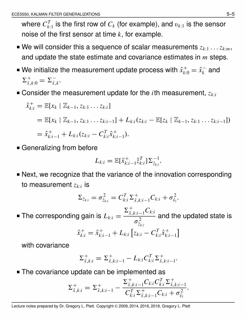
� An alternative update is the Joseph form,

�+x,k:i = [

I − Lk:iC Tk:i

]�+

x,k:i

[I − Lk:iC T

k:i

]T + Lk:iσ2vi

LTk:i .

� The final measurement update gives x+k = x+

k:m and �+x,k = �+

x,k:m.

Sequentially processing correlated measurements

� The above process must be modified to accommodate the situationwhere sensor noise is correlated among the measurements.

� Assume that we can factor the matrix �v = SvSTv , where Sv is a

lower-triangular matrix (for symmetric positive-definite �v , we can).

• The factor Sv is a kind of a matrix square root, and will beimportant in a number of places in this course.

• It is known as the “Cholesky” factor of the original matrix.

• In MATLAB, Sv = chol(SigmaV,'lower');

• Be careful: MATLAB’s default answer (without specifying “lower”)is an upper-triangular matrix, which is not what we’re after.

� The Cholesky factor has strictly positive elements on its diagonal(positive eigenvalues), so is guaranteed to be invertible.

� Consider a modification to the output equation of a system havingcorrelated measurements

zk = Cxk + vk

zk = S−1v zk = S−1

v Cxk + S−1v vk

zk = C xk + vk.

• Note that we will use the “bar” decoration (·) frequently in thischapter of notes.



• It rarely (if ever) indicates the mean of that quantity.

• Rather, it refers to a definition having similar meaning to theoriginal symbol.

• For example, zk is a (computed) output value, similar ininterpretation to the measured output value zk.

� Consider now the covariance of the modified noise input vk = S−1v vk

� ˜vk= E[vk v

Tk ]

= E[S−1v vkv

Tk S−T

v ]

= S−1v �vS−T

v = I .

� Therefore, we have identified a transformation that de-correlates (andnormalizes) measurement noise.

� Using this revised output equation, we use the prior method.

� We start the measurement update process with x+k:0 = x−

k and�+

x,k:0 = �−x,k.

� The Kalman gain is Lk:i = �+x,k:i−1Ck:i

C Tk:i�

+x,k:i−1Ck:i + 1

and the updated state is

x+k:i = x+

k:i−1 + Lk:i[zk:i − C T

k:i x+k:i−1

]= x+

k:i−1 + Lk:i[(S−1

v zk)i − C Tk:i x

+k:i−1

].

with covariance

�+x,k:i = �+

x,k:i−1 − Lk:i C Tk:i�

+x,k:i−1

(which may also be computed with a Joseph form update, forexample).

� The final measurement update gives x+k = x+

k:m and �+x :k = �+

x,k:m.



LDL updates for correlated measurements

� An alternative to the Cholesky decomposition for factoring thecovariance matrix is the LDL decomposition

�v = LvDvLTv ,

where Lv is lower-triangular and Dv is diagonal (with positive entries).

� In MATLAB, [L,D] = ldl(SigmaV);

� The Cholesky decomposition is related to the LDL decomposition via

Sv = LvD1/2v .

� Both texts show how to use the LDL decomposition to perform asequential measurement update.

� A computational advantage of LDL over Cholesky is that nosquare-root operations need be taken. (We can avoid finding D1/2

v .)

� A pedagogical advantage of introducing the Colesky decomposition isthat we use it later on.



5.3: Square-root filtering

� The modifications to the basic Kalman filter that we have describedso far are able to

• Ensure symmetric, positive-definite covariance matrices;

• Speed up the operation of a multiple-measurement Kalman filter.

� The filter is still sensitive to finite word length: no longer in the senseof causing divergence, but in the sense of not converging to as gooda solution as possible.

� Consider the set of numbers: 1,000,000; 100; 1. There are six ordersof magnitude in the spread between the largest and smallest.

� Now consider a second set of numbers: 1,000; 10; 1. There are onlythree orders of magnitude in spread.

� But, the second set is the square root of the first set: We can reducedynamic range (number of bits required to implement a givenprecision of solution) by using square roots of numbers.

� For example, we can get away with single-precision math instead ofdouble-precision math.

� The place this really shows up is in the eigenvalue spread ofcovariance matrices. If we can use square-root matrices instead, thatwould be better.

� Consider the Cholesky factorization from before. Define

�+x,k = S+

x,k

(S+

x,k

)Tand �−

x,k = S−x,k

(S−

x,k

)T.



� We would like to be able to compute the covariance time updates andmeasurement updates in terms of S±

x,k instead of �±x,k. Let’s take the

steps in order.

SR-KF step 1a: State estimate time update.

� We computex−

k = Ak−1x+k−1 + Bk−1uk−1.

� No change in this step from standard KF.

SR-KF step 1b: Error covariance time update.

� We start with standard step

�−x,k = Ak−1�

+x,k−1 AT

k−1 + �w.

� We would like to write this in terms of Cholesky factors

S−x,k

(S−

x,k

)T = Ak−1S+x,k−1

(S+

x,k−1

)TAT

k−1 + SwSTw .

� One option is to compute the right side, then take the Choleskydecomposition to compute the factors on the left side. This iscomputationally too intensive.

� Instead, start by noticing that we can write the equation as

S−x,k

(S−

x,k

)T =[

Ak−1S+x,k−1, Sw

] [Ak−1S+

x,k−1, Sw

]T

= M MT .

� This might at first appear to be exactly what we desire, but theproblem is that S−

x,k is and n ×n matrix, whereas M is an n ×2n matrix.

� But, it is at least a step in the right direction. Enter the QRdecomposition.



QR decomposition: The QR decomposition algorithm computes twofactors Q ∈ R

n×n and R ∈ Rn×m for a matrix Z ∈ R

n×m such thatZ = Q R, Q is orthogonal, R is upper-triangular, and m ≥ n.

� The property of the QR factorization that is important here is that R isrelated to the Cholesky factor we wish to find.

� Specifically, if R ∈ Rn×n is the upper-triangular portion of R, then RT is

the Cholesky factor of � = MT M.

� That is, if R = qr(MT )T , where qr(·) performs the QR decompositionand returns the upper-triangular portion of R only, then R is thelower-triangular Cholesky factor of M MT .

� Continuing with our derivation, notice that if we form M as above,then compute R, we have our desired result.

S−x,k = qr

([Ak−1S+

x,k−1, Sw

]T)T

.

� The computational complexity of the QR decomposition is O(mn2),whereas the complexity of the Cholesky factor is O(n3/6) plus O(mn2)

to first compute M MT .

� In MATLAB:

Sminus = qr([A*Splus,Sw]')';

Sminus = tril(Sminus(1:nx,1:nx));

SR-KF step 1c: Estimate system output.

� As before, we estimate the system output as

zk = Ckx−k + Dkuk.

SR-KF step 2a: Estimator (Kalman) gain matrix.



� In this step, we must compute Lk = �−x z,k(�z,k)

−1.

� Recall that �−x z,k = �−

x,kC Tk and �z,k = Ck�

−x,kC T

k + �v .

� We may find Sz,k using the QR decomposition, as before. And, wealready know S−

x,k.

� So, we can now write Lk(Sz,kSTz,k) = �−

x z,k.

� If zk is not a scalar, this equation may often be computed mostefficiently via back-substitution in two steps.

• First, (M)STz,k = �−

x z,k is found, and

• Then LkSz,k = M is solved.

• Back-substitution has complexity O(n2/2).

• Since Sz,k is already triangular, no matrix inversion need be done.

� Note that multiplying out �−x,k = S−

x,k

(S−

x,k

)Tin the computation of

�−x z,k may drop some precision in Lk.

� However, this is not the critical issue.

� The critical issue is keeping S±x,k accurate for whatever Lk is used,

which is something that we do manage to accomplish.

� In MATLAB:

Sz = qr([C*Sminus,Sv]')';

Sz = tril(Sz(1:nz,1:nz));

L = (Sminus*Sminus')*C'/Sz'/Sz;

SR-KF step 2b: State estimate measurement update.

� This is done just as in the standard Kalman filter,

x+k = x−

k + Lk(zk − zk).



SR-KF step 2c: Error covariance measurement update.

� Finally, we update the error covariance matrix.

�+x,k = �−

x,k − Lk�z,k LTk ,

which can be written as,

S+x,k

(S+

x,k

)T = S−x,k

(S−

x,k

)T − LkSzSTz LT

k .

� Note that the “−” sign prohibits us using the QR decomposition tosolve this problem as we did before.

� Instead, we rely on the “Cholesky downdating” procedure.

� In MATLAB,

% deal with MATLAB wanting upper-triangular Cholesky factor

Sx_ = Sminus';

% Want SigmaPlus = SigmaMinus - L*Sigmaz*L';

cov_update_vectors = L*Sz;

for j=1:length(zhat),

Sx_ = cholupdate(Sx_,cov_update_vectors(:,j),'-');

end

% Re-transpose to undo MATLAB's strange Cholesky factor

Splus = Sx_';

� If you need to implement this kind of filter in a language other thanMATLAB, a really excellent discussion of finding Cholesky factors, QRfactorizations, and both Cholesky updating and downdating may befound in: G.W. Stewart, Matrix Algorithms, Volume I: BasicDecompositions, Siam, 1998. Pseudo-code is included.



Summary of the square-root linear Kalman filter

Linear state-space model:xk = Ak−1xk−1 + Bk−1uk−1 + wk−1

zk = Ck xk + Dkuk + vk,

where wk and vk are independent, zero-mean, Gaussian noise processes of

covariance matrices �w and �v , respectively.

Initialization: For k = 0, set

x+0 =E[x0] Sw = chol(�w, 'lower').

�+x,0 =E[(x0 − x+

0 )(x0 − x+0 )T ]. Sv = chol(�v, 'lower').

S+x,0 =chol(�+

x,0, 'lower').

Computation: For k = 1, 2, . . . compute:

State estimate time update: x−k = Ak−1x+

k−1 + Bk−1uk−1.

Error covariance time update: S−x,k =cholupdate

((Ak−1S+

x,k−1

)T,ST

w

)T

.

Output estimate: zk = Ckx−k + Dkuk.

Estimator gain matrix:∗ Sz,k =cholupdate

((CkS−

x,k

)T,ST

v

)T

.

MSTz,k =S−

x,k

(S−

x,k

)TCT

k , (solved by backsubstitution)

LkSz,k = M , (solved by backsubstitution)

State estimate meas. update: x+k = x−

k + Lk(zk − zk).

Error covariance meas. update: S+x,k =cholupdate

((S−

x,k

)T,(LkSz,k

)T, '-'

)T

.

∗If a measurement is missed for some reason, then simply skip the measurement update for that iteration.That is, Lk = 0 and x+

k = x−k and S+

x,k = S−x,k.



5.4: MATLAB code for the square-root Kalman filter steps

� Coding a square-root Kalman filter in MATLAB is straightforward.

% Initialize simulation variables

SRSigmaW = chol(1,'lower'); % Square-root process noise covar

SRSigmaV = chol(1,'lower'); % Square-root sensor noise covar

A = 1; B = 1; C = 1; D = 0; % Plant definition matrices

maxIter = 40;

xtrue = 0; xhat = 0 % Initialize true and estimated system initial state

SigmaX = 0.1; % Initialize Kalman filter covariance

SRSigmaX = chol(SigmaX,'lower');

u = 0; % Unknown initial driving input: assume zero

% Reserve storage for variables we might want to plot/evaluate

xstore = zeros(maxIter+1,length(xtrue)); xstore(1,:) = xtrue;

xhatstore = zeros(maxIter,length(xhat));

SigmaXstore = zeros(maxIter,length(xhat)); % store diagonal only

for k = 1:maxIter,

% SR-KF Step 1a: State estimate time update

xhat = A*xhat + B*u; % use prior value of "u"

% SR-KF Step 1b: Error covariance time update

SRSigmaX = qr([A*SRSigmaX, SRSigmaW]')';

SRSigmaX = tril(SRSigmaX(1:length(xhat),1:length(xhat)));

% [Implied operation of system in background, with

% input signal u, and output signal z]

u = 0.5*randn(1) + cos(k/pi); % for example... (measured)

w = SRSigmaW*randn(length(xtrue));

v = SRSigmaV*randn(length(C*xtrue));

ztrue = C*xtrue + D*u + v; % y is based on present x and u

xtrue = A*xtrue + B*u + w; % future x is based on present u

% SR-KF Step 1c: Estimate system output

zhat = C*xhat + D*u;

% SR-KF Step 2a: Compute Kalman gain matrix

% Note: "help mrdivide" to see how "division" is implemented

SRSigmaZ = qr([C*SRSigmaX,SRSigmaV]')';

SRSigmaZ = tril(SRSigmaZ(1:length(zhat),1:length(zhat)));



L = (SRSigmaX*SRSigmaX')*C'/SRSigmaZ'/SRSigmaZ;

% SR-KF Step 2b: State estimate measurement update

xhat = xhat + L*(ztrue - zhat);

% SR-KF Step 2c: Error covariance measurement update

Sx_ = SRSigmaX';

cov_update_vectors = L*SRSigmaZ;

for j=1:length(zhat),

Sx_ = cholupdate(Sx_,cov_update_vectors(:,j),'-');

end

SRSigmaX = Sx_';

% [Store information for evaluation/plotting purposes]

xstore(k+1,:) = xtrue; xhatstore(k,:) = xhat;

SigmaXstore(k,:) = diag(SRSigmaX*SRSigmaX');

end;

figure(1); clf;

plot(0:maxIter-1,xstore(1:maxIter),'k-',0:maxIter-1,xhatstore,'b--', ...

0:maxIter-1,xhatstore+3*sqrt(SigmaXstore),'m-.',...

0:maxIter-1,xhatstore-3*sqrt(SigmaXstore),'m-.'); grid;

title('Kalman filter in action'); xlabel('Iteration');

ylabel('State'); legend('true','estimate','bounds');

figure(2); clf;

plot(0:maxIter-1,xstore(1:maxIter)-xhatstore,'b-', ...

0:maxIter-1,3*sqrt(SigmaXstore),'m--',...

0:maxIter-1,-3*sqrt(SigmaXstore),'m--');

grid; legend('Error','bounds',0); title('Error with bounds');

xlabel('Iteration'); ylabel('Estimation Error');

0 5 10 15 20 25 30 35 40−10

−5

0

5

10

15

trueestimatebounds

Iteration

Sta

te

Kalman filter in action

0 5 10 15 20 25 30 35 40−3

−2

−1

0

1

2

3

Errorbounds

Iteration

Est

imat

ion

Err

or

Error with bounds



5.5: Cross-correlated process and measurement noises: Coincident

� The standard KF assumes that E[wkvTj ] = 0. But, sometimes we may

encounter systems where this is not the case.

� This might happen if both the physical process and the measurementsystem are affected by the same source of disturbance. Examplesare changes of temperature, or inductive electrical interference.

� In this section, we assume that E[wkwTj ] = �wδk j , E[vkv

Tj ] = �vδk j ,

and E[wkvTj ] = �wvδk j .

� Note that the correlation between noises is memoryless: the onlycorrelation is at identical time instants.

� We can handle this case if we re-write the plant equation so that it hasa new process noise that is uncorrelated with the measurement noise.

� Using an arbitrary matrix T (to be determined), we can write

xk+1 = Akxk + Bkuk + wk + T (zk − Ckxk − Dkuk − vk)

= (Ak − T Ck)xk + (Bk − T Dk)uk + wk − T vk + T zk.

� Denote the new transition matrix Ak = Ak − T Ck, new input matrix asBk = Bk − T Dk, and the new process noise as wk = wk − T vk.

� Further, denote the known (measured/computed) sequence as a newinput uk = T zk.

� Then, we can write a modified state space system

xk+1 = Akxk + Bkuk + uk + wk.

� We can create a Kalman filter for this system, provided that thecross-correlation between the new process noise wk and the sensor



noise vk is zero. We enforce this:

E[wkvTk ] = E

[[wk − T vk]vT

k

] = �wv − T �v = 0.

� This gives us that the previously unspecified matrix T = �wv�−1v .

� Using the above, the covariance of the new process noise may befound to be

�˜w = E[wkwTk ]

= E

[[wk − �wv�

−1v vk

] [wk − �wv�

−1v vk

]T]

= �w − �wv�−1v �T

wv .

� A new Kalman filter may be generated using these definitions:

Ak = Ak − �wv�−1v Ck

�˜w = �w − �wv�−1v �T

wv ,

and

xk+1 = (Ak − �wv�−1v Ck)xk + (Bk − �wv�

−1v Dk)uk + �wv�

−1v zk + wk

zk = Ckxk + Dkuk + vk.

Cross-correlated process and measurement noises: Shifted

� A close relation to the above is when the process noise and sensornoise have correlation one timestep apart.

� That is, we assume that E[wkwTj ] = �wδk j , E[vkv

Tj ] = �vδk j , and

E[wkvTj ] = �wvδk, j−1. The cross-correlation is nonzero only between

wk−1 and vk.

� We can re-derive the KF equations using this assumption. We willfind that the differences show up in the state-error covariance terms.



� The state prediction error is

x−k = xk − x−

k = Akx+k−1 + wk−1.

� With the assumptions of this section, the covariance between thestate prediction error and the measurement noise is

E[x−k vT

k ] = E

[[Akx+

k−1 + wk−1]vTk

] = �wv .

� The covariance between the state and the measurement becomes

E

[x−

k zTk | Zk−1

] = E

[x−

k

(Ckx−

k + vk)T | Zk−1

]= �−

x,kC Tk + �wv.

� The measurement prediction covariance becomes

�z,k = E

[zk zT

k

]= E

[[Ckx−

k + vk][Ckx−k + vk]T ]

= Ck�−x,kC T

k + �v + Ck�wv + �TwvC T

k .

� The modified KF gain then becomes,

Lk =[�−

x,kC Tk + �wv

] (Ck�

−x,kC T

k + �v + Ck�wv + �TwvC T

k

)−1.

� Except for the modified filter gain, all of the KF equations are thesame as in the standard case.

� Note that since wk−1 is the process noise corresponding to the interval[tk−1, tk] and v j is the measurement noise at t j , it can be seen that thefirst case considered process noise correlated with measurementnoise at the beginning of the above interval, and the second caseconsidered process noise correlated with the end of the interval.



Auto-correlated process noise

� Another common situation that contradicts the KF assumptions is thatthe process noise is correlated in time.

� That is, with the standard assumption that xk+1 = Akxk + Bkuk + wk,we do not have zero-mean white-noise wk.

� Instead, we have wk = Awwk−1 + wk−1, where wk−1 is a zero-meanwhite-noise process.

� We handle this situation by estimating both the true system state xk

and also the noise state wk. We have[xk

wk

]=

[Ak−1 I

0 Aw

] [xk−1

wk−1

]+

[Bk−1

0

]uk−1 +

[0

wk−1

]x∗

k = A∗k−1x∗

k−1 + B∗k−1uk−1 + w∗

k−1,

where the overall process noise covariance is

�w∗ = E[w∗k−1(w

∗k−1)

T ] =[

0 00 E[wk−1 (wk−1)

T ]

]and the output equation is

zk =[

Ck 0] [

xk

wk

]+ Dkuk + vk

= C∗k x∗

k + Dkuk + vk.

� A standard Kalman filter may now be designed using the definitions ofx∗

k , A∗k, B∗

k , C∗k , Dk, �w∗, and �v.

Auto-correlated sensor noise

� Similarly, we might encounter situations with auto-correlated sensornoise: vk = Avvk−1 + vk−1, where vk is white.



� We take a similar approach. The augmented system is[xk

vk

]=

[Ak−1 0

0 Av

] [xk−1

vk−1

]+

[Bk−1

0

]uk−1 +

[wk−1

vk−1

]x∗

k = A∗k−1x∗

k−1 + B∗k−1uk−1 + w∗

k−1

with output equation

zk =[

Ck I] [

xk

vk

]+ Dkuk + 0

= C∗k x∗

k + Dkuk + 0

� The covariance of the combined process noise is

�w∗ = E

[(wk

vk

)(wk vk

)]=

[�w 00 � ˜v

].

� A Kalman filter may be designed using these new definitions of of x∗k ,

A∗k, B∗

k , C∗k , Dk, �w∗, with �v = 0 (the placeholder for measurement

noise is zero in the above formulations).

Measurement differencing

� Zero-covariance measurement noise can cause numerical issues.

� A sneaky way to fix this is to introduce an artificial measurement thatis computed as a scaled difference between two actualmeasurements: zk = zk+1 − Avzk.

� KF equations can then be developed using this new “measurement.”

� The details are really messy and not conducive to a lecturepresentation. I refer you to Bar-Shalom!

� Care must be taken to deal with the “future” measurement zk+1 in theupdate equations, but it works out to a causal solution in the end.



5.6: Kalman-filter prediction and smoothing

� Prediction is the estimation of the system state at a time m beyondthe data interval. That is,

x−m|k = E[xm | Zk],

where m > k.

� There are three different prediction scenarios:

• Fixed-point prediction: Find x−m|k where m is fixed, but k is changing

as more data becomes available;

• Fixed-lead prediction: Find x−k+L|k where L is a fixed lead time;

• Fixed-interval prediction: Find x−m|k where k is fixed, but m can take

on multiple future values.

� The desired predictions can be extrapolated from the standardKalman filter state and estimates.

� The basic approach is to use the relationship (cf. Homework 1)

xm =m−k−1∏

j=0

Am−1− j

xk +m−1∑i=k

m−i−2∏j=0

Am−1− j

Biui

+m−1∑i=k

m−i−2∏j=0

Am−1− j

wi ,

in the relationshipx−

m|k = E[xm | Zk],

with the additional knowledge that x+k = E[xk | Zk] from a standard

Kalman filter.



� That is,

x−m|k = E[xm | Zk]

= E

m−k−1∏j=0

Am−1−i

xk | Zk

+ E

m−1∑i=k

m−i−2∏j=0

Am−1−i

Biui | Zk

+E

m−1∑i=k

m−i−2∏j=0

Am−1− j

wi | Zk

=

m−k−1∏j=0

Am−1−i

x+k +

m−1∑i=k

m−i−2∏j=0

Am−1−i

BiE[ui | Zk].

� Note that we often assume that E[uk] = 0.

� If, furthermore, the system is time invariant,

x−m|k = Am−k x+

k .

� The covariance of the prediction is

�−x,m|k = E[(xm − x−

m|k)(xm − x−m|k)

T | Zk]

=m−k−1∏

j=0

Am−1−i

�+x,k

m−k−1∏j=0

Am−1−i

T

+m−1∑i=k

m−i−2∏j=0

Am−1− j

�w

m−i−2∏j=0

ATm−1− j

.

� If the system is time invariant, this reduces to

�−x,m|k = Am−k�+

x,k

(Am−k)T +

m−k∑j=1

A j�w

(A j)T .



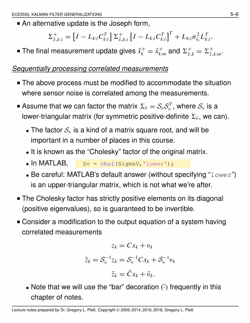
Smoothing

� Smoothing is the estimation of the system state at a time m amid thedata interval. That is,

x+m|N = E[xm | ZN ],

where m < N .

� There are three different smoothing scenarios:

• Fixed-point smoothing: Find x+m|k where m is fixed, but k is

changing as more data becomes available;

• Fixed-lag smoothing: Find x−k−L|k where L is a fixed lag time;

• Fixed-interval smoothing: Find x+m|N where k is fixed, but m can

take on multiple past values.

� Of these, fixed-interval smoothing is the most relevant, and both textshave detailed derivations.

� The others use a variation of this idea.

Fixed interval smoothing

� The algorithm consists of a forward recursive pass followed by abackward pass.

� The forward pass uses a Kalman filter, and saves the intermediateresults x−

k , x+k , �−

x,k, and �+x,k.

� The backward pass starts at time N of the last measurement, andcomputes the smoothed state estimate using the results obtainedfrom the forward pass.



� Recursive equations (backward sweep)

x+m|N = x+

m + λm

(x+

m+1|N − x−m+1

)λm = �+

x,m ATm

(�−

x,m+1

)−1

where m = N − 1, N − 2, . . . , 0. Note, x+N |N = x+

N to start backwardpass.

� The error covariance matrix for the smoothed estimate is

�+x,m|N = �+

x,m + λm

[�+

x,m+1|N − �−x,m+1

]λT

m,

but it is not needed to be able to perform the backward pass.

� Note, the term in the square brackets is negative semi-definite, so thecovariance of the smoothed estimate is “smaller” than for the filteredestimate only.

Fixed point smoothing

� Here, m is fixed, and the final point k keeps increasing.

x+m|k = x+

m|k−1 + µk(x+

k − x−k

)µk =

k−1∏i=m

λi ,

where the product multiplies on the left as i increases.

� For k = m + 1,

x+m|m+1 = x+

m + µm+1(x+

m+1 − x−m+1

)µm+1 = λm = �+

x,m ATm

(�−

x,m+1

)−1.



� For k = m + 2,

x+m|m+2 = x+

m|m+1 + µm+2(x+

m+2 − x−m+2

)µm+2 = �+

x,m+1 ATm+1

(�−

x,m+2

)−1µk+1,

and so forth.

Fixed lag smoothing

� Here, we seek to estimate the state vector at a fixed time intervallagging the time of the current measurement.

� This type of smoothing trades off estimation latency for moreaccuracy.

� The fixed interval smoothing algorithm could be used to performfixed-lag smoothing when the number of backward steps equals thetime lag

� This is fine as long as the number of backward steps is small.

� Fixed-lag smoothing algorithm has a startup problem: Cannot rununtil enough data is available.



5.7: Reduced-order Kalman filter

� Why estimate the entire state vector when you are measuring one ormore state elements directly?

� Consider partitioning system state into (may require transformation)

xk:a : measured state

xk:b : to be estimated.

� So,

zk = Cxk + Duk + vk = xk:a + Duk + vk

xk:a = zk − Duk = xk:a + vk.

� We assume that the measurement is noise-free (otherwise, we wouldneed to estimate xk:a also). So, xk:a = zk − Duk = xk:a.

� In order to design an estimator for xk:b, we need to create a suitablestate-space model of the dynamics of xk:b.

� We begin by writing the equations for the partitioned system

[xk+1:a

xk+1:b

]=

[Aaa Aab

Aba Abb

] [xk:a

xk:b

]+

[Ba

Bb

]uk +

[wk:a

wk:b

]

zk =[

I 0] [

xk:a

xk:b

]+ Duk.

� We wish to write the xk:b dynamics in the form:

xk+1:b = Axbxk:b + Bxbmk,1 + wk



mk,2 = Cxbxk:b + Dxbmk,1 + vk,

where mk,1 and mk,2 are some measurable inputs, and will becombinations of zk and uk.

• Once we have this state-space form, we can create a Kalman-filterstate estimator for xk:b.

� We start the derivation by finding an output equation for xk:b. Considerthe dynamics of the measured state:

xk+1:a = Aaaxk:a + Aabxk:b + Bauk + wk:a

zk+1 = Aaazk + Aabxk:b + Bauk + wk:a.

� Letmk,2 = zk+1 − Aaazk − Bauk.

� Thenmk,2 = Aabxk:b + wk:a,

where mk,2 is known/measurable and thus “Cxb” is equal to Aab.

• This is our reduced-order estimator output relation.

� We now look for a state equation for xk:b. Consider the dynamics ofthe estimated state:

xk+1:b = Abaxk:a + Abbxk:b + Bbuk + wk:b

Abbxk:b + Abazk + Bbuk + wk:b.

� LetBxbmk,1 = Abazk + Bbuk

so that the reduced-order recurrence relation is

xk+1:b = Abbxk:b + Bxbmk,1 + wk:b.



� This might be accomplished via

Bxbmk,1 =[

Aba Bb

] [zk

uk

]although the details of how this is done do not matter in the end.

� So, for the purpose of designing our estimator, the state-spaceequations are:

xk+1:b = Abbxk:b + Bxbmk,1 + wk

mk,2 = Aabxk:b + vk,

where wk = wk:b and vk = wk:a.

� Note that the measurement is non-causal, so the filter output will lagthe true output by one sample.

� Another (causal) approach that does not assume noise-freemeasurements is presented in: D. Simon, “Reduced Order KalmanFiltering without Model Reduction,” Control and Intelligent Systems,vol. 35, no. 2, pp. 169–174, April 2007.

� This algorithm can end up more complicated than full Kalman filterunless many states are being removed from estimation requirements.



5.8: Measurement validation gating

� Sometimes the systems for which we would like a state estimate havesensors with intermittent faults.

� We would like to detect faulty measurements and discard them (thetime update steps of the KF are still implemented, but themeasurement update steps are skipped).

� The Kalman filter provides an elegant theoretical means toaccomplish this goal. Note:

• The measurement covariance matrix is �z,k = Ck�−x,kC T

k + �v ;

• The measurement prediction itself is zk = Ckx−k + Dkuk;

• The innovation is zk = zk − zk.

� A measurement validation gate can be set up around themeasurement using normalized estimation error squared (NEES)

e2k = zT

k �−1z,k zk.

� NEES e2k varies as a Chi-squared distribution with m degrees of

freedom, where m is the dimension of zk.

� If e2k is outside the bounding values from the Chi-squared distribution

for a desired confidence level, the measurement is discarded.

� Note: If a number of measurements are discarded in a short timeinterval, it may be that the sensor has truly failed, or that the stateestimate and its covariance has gotten “lost.”

� It is sometimes helpful to “bump up” the covariance �±x,k, which

simulates additional process noise, to help the Kalman filter toreacquire.



Chi-squared test

� A chi-square random variable is defined as a sum of squares ofindependent unit variance zero mean normal random variables.

Y =n∑

i=1

(Xi − E[Xi]

σ

)2

.

� Y is chi-square with n degrees of freedom.

� Since it is a sum of squares, it is never negative and is notsymmetrical about its mean value.

� The pdf of Y with n degrees of freedom is

fY (y) = 12n/2�(n/2)

y(n/2−1)e−n/2.

� For confidence interval estimation we need to find two critical values.

10 20 30 40 50

0.01

0.02

0.03

0.04

0.05

0.06

χ�

�χ�

�

12.401 39.364

Total Area = 0.95

Tail = 0.05/2 = 0.025

χ��

�

��

Critical values for 95% confidence and χ2 with 24 degrees of freedom

� If we want 1 − α confidence that the measurement is valid, we want tomake sure that Y is between χ2

L and χ2U where χ2

L is calculated usingα/2 and χ2

U is calculated using 1 − α/2.



� The χ2 pdf, cdf, and inverse cdf are available in most analysissoftware packages (e.g., MATLAB, Mathematica, and even thespreadsheet program Excel).

� For hand calculations a χ2-table is available on page ??.

TRICKS WITH MATLAB: MATLAB may also be used to find the χ2 values ifa table is not convenient. This requires the MATLAB statistics toolbox:

>> help chi2inv

CHI2INV Inverse of the chi-square cumulative distribution function (cdf).

X = CHI2INV(P,V) returns the inverse of the chi-square cdf with V

degrees of freedom at the values in P. The chi-square cdf with V

degrees of freedom, is the gamma cdf with parameters V/2 and 2.

The size of X is the common size of P and V. A scalar input

functions as a constant matrix of the same size as the other input.

>> % want to compute values for alpha = 0.05

>> chi2inv(1-.025,24) % Tail probability of alpha/2=0.025, n = 24. Upper

critical value

ans = 39.3641

>> chi2inv(.025,24) % Lower critical value

ans = 12.4012



Appendix: Critical Values of χ2

� For some deg. of freedom, each entryrepresents the critical value of χ2 for aspecified upper tail area α.

0 χ2U (α,df)

α1 − α

Deg

rees

ofU

pper

Tail

Are

asFr

eedo

m0.995

0.99

0.975

0.95

0.90

0.75

0.25

0.10

0.05

0.025

0.01

0.005

10.000

0.000

0.001

0.004

0.016

0.102

1.323

2.706

3.841

5.024

6.635

7.879

20.010

0.020

0.051

0.103

0.211

0.575

2.773

4.605

5.991

7.378

9.210

10.597

30.072

0.115

0.216

0.352

0.584

1.213

4.108

6.251

7.815

9.348

11.345

12.838

40.207

0.297

0.484

0.711

1.064

1.923

5.385

7.779

9.488

11.143

13.277

14.860

50.412

0.554

0.831

1.145

1.610

2.675

6.626

9.236

11.070

12.833

15.086

16.750

60.676

0.872

1.237

1.635

2.204

3.455

7.841

10.645

12.592

14.449

16.812

18.548

70.989

1.239

1.690

2.167

2.833

4.255

9.037

12.017

14.067

16.013

18.475

20.278

81.344

1.646

2.180

2.733

3.490

5.071

10.219

13.362

15.507

17.535

20.090

21.955

91.735

2.088

2.700

3.325

4.168

5.899

11.389

14.684

16.919

19.023

21.666

23.589

10

2.156

2.558

3.247

3.940

4.865

6.737

12.549

15.987

18.307

20.483

23.209

25.188

11

2.603

3.053

3.816

4.575

5.578

7.584

13.701

17.275

19.675

21.920

24.725

26.757

12

3.074

3.571

4.404

5.226

6.304

8.438

14.845

18.549

21.026

23.337

26.217

28.300

13

3.565

4.107

5.009

5.892

7.042

9.299

15.984

19.812

22.362

24.736

27.688

29.819

14

4.075

4.660

5.629

6.571

7.790

10.165

17.117

21.064

23.685

26.119

29.141

31.319

15

4.601

5.229

6.262

7.261

8.547

11.037

18.245

22.307

24.996

27.488

30.578

32.801

16

5.142

5.812

6.908

7.962

9.312

11.912

19.369

23.542

26.296

28.845

32.000

34.267

17

5.697

6.408

7.564

8.672

10.085

12.792

20.489

24.769

27.587

30.191

33.409

35.718

18

6.265

7.015

8.231

9.390

10.865

13.675

21.605

25.989

28.869

31.526

34.805

37.156

19

6.844

7.633

8.907

10.117

11.651

14.562

22.718

27.204

30.144

32.852

36.191

38.582

20

7.434

8.260

9.591

10.851

12.443

15.452

23.828

28.412

31.410

34.170

37.566

39.997

21

8.034

8.897

10.283

11.591

13.240

16.344

24.935

29.615

32.671

35.479

38.932

41.401

22

8.643

9.542

10.982

12.338

14.041

17.240

26.039

30.813

33.924

36.781

40.289

42.796

23

9.260

10.196

11.689

13.091

14.848

18.137

27.141

32.007

35.172

38.076

41.638

44.181

24

9.886

10.856

12.401

13.848

15.659

19.037

28.241

33.196

36.415

39.364

42.980

45.559

25

10.520

11.524

13.120

14.611

16.473

19.939

29.339

34.382

37.652

40.646

44.314

46.928

26

11.160

12.198

13.844

15.379

17.292

20.843

30.435

35.563

38.885

41.923

45.642

48.290

27

11.808

12.879

14.573

16.151

18.114

21.749

31.528

36.741

40.113

43.195

46.963

49.645

28

12.461

13.565

15.308

16.928

18.939

22.657

32.620

37.916

41.337

44.461

48.278

50.993

29

13.121

14.256

16.047

17.708

19.768

23.567

33.711

39.087

42.557

45.722

49.588

52.336

30

13.787

14.953

16.791

18.493

20.599

24.478

34.800

40.256

43.773

46.979

50.892

53.672

31

14.458

15.655

17.539

19.281

21.434

25.390

35.887

41.422

44.985

48.232

52.191

55.003

32

15.134

16.362

18.291

20.072

22.271

26.304

36.973

42.585

46.194

49.480

53.486

56.328

33

15.815

17.074

19.047

20.867

23.110

27.219

38.058

43.745

47.400

50.725

54.776

57.648

34

16.501

17.789

19.806

21.664

23.952

28.136

39.141

44.903

48.602

51.966

56.061

58.964

35

17.192

18.509

20.569

22.465

24.797

29.054

40.223

46.059

49.802

53.203

57.342

60.275

36

17.887

19.233

21.336

23.269

25.643

29.973

41.304

47.212

50.998

54.437

58.619

61.581

37

18.586

19.960

22.106

24.075

26.492

30.893

42.383

48.363

52.192

55.668

59.893

62.883

38

19.289

20.691

22.878

24.884

27.343

31.815

43.462

49.513

53.384

56.896

61.162

64.181

39

19.996

21.426

23.654

25.695

28.196

32.737

44.539

50.660

54.572

58.120

62.428

65.476

40

20.707

22.164

24.433

26.509

29.051

33.660

45.616

51.805

55.758

59.342

63.691

66.766

45

24.311

25.901

28.366

30.612

33.350

38.291

50.985

57.505

61.656

65.410

69.957

73.166

50

27.991

29.707

32.357

34.764

37.689

42.942

56.334

63.167

67.505

71.420

76.154

79.490


Documents

KALMAN FILTER GENERALIZATIONSmocha-java.uccs.edu/ECE5550/ECE5550-Notes05.pdf · 2018-08-20 · ECE5550, KALMAN FILTER GENERALIZATIONS 5–9 5.3: Square-root ﬁltering The modiﬁcations