Proceedings of the 2020 Winter Simulation ConferenceK.-H. Bae, B. Feng, S. Kim, S. Lazarova-Molnar, Z. Zheng, T. Roeder, and R. Thiesing, eds.

SCHEDULING QUEUES WITH SIMULTANEOUS AND HETEROGENEOUS REQUIREMENTSFROM MULTIPLE TYPES OF SERVERS

Noa Zychlinski

Industrial Engineering and ManagementTechnion Institute of Technology

Haifa 32000, ISRAEL

Carri W. ChanJing Dong

Graduate School of BusinessColumbia University

New York, NY 10027, USA

ABSTRACT

We study the scheduling of a new class of multi-class multi-pool queueing systems where different classesof customers have heterogeneous – in terms of the type and amount – resource requirements. In particular, acustomer may require different numbers of servers from different server pools to be allocated simultaneouslyin order to be served. We apply stochastic simulation to study properties of the model and identify twotypes of server idleness: avoidable and unavoidable idleness, which play important, but different, roles indictating system performance, and need to be carefully managed in scheduling. To minimize the long-runaverage holding cost, we propose a generalization of the cµ-rule, called Generalized Idle-Aware (GIA)cµ-rule. We provide insights into how to set the hyper parameters of the GIA cµ-rule. We also demonstratethat, with properly chosen hyper parameters, the GIA cµ-rule achieves superior and robust performancecompared to reasonable benchmarks.

1 INTRODUCTION

In this paper, we develop a special parallel processing network with multiple types of resources and multipleclasses of customers. Each class of customers can require multiple types and/or multiple units of resourcessimultaneously to get served. This model is relevant for many operations management applications. Forexample, in healthcare systems, patients are classified based on the level of medical attention/supervisionthey require. Each class of patients requires multiple types of resources (physicians/nurses/beds/medicalequipment), as well as, a different amount of each type of resources. In an Intensive Care Unit (ICU), highacuity patients typically require one dedicated nurse per patient; however, the same nurse can take care oftwo to three ICU patients at lower acuity levels (Masterson and Baudouin 2015). We need both a bed andthe required staff to admit a patient. Other examples include emergency services such as firefighting andpolice patrol (Altay 2012); manufacturing, and inventory systems (Ramakrishnan and Gannon 2008).

We study the scheduling of the proposed model, with the objective of minimizing the long-run averageholding cost. Due to the complex architecture and dynamics of the proposed network model, very fewanalytical results can be derived. In this context, discrete-even simulation is the main tool for performanceevaluation and optimization of these systems (Glynn and Asmussen 2007).

The heterogenous resource requirements pose challenges on managing priority-induced idleness. Inparticular, policies that myopically maximize the cost-reduction rate may lead to system instability, evenif the system can be stabilized under some properly designed policies. In this work, we identify two typesof idleness: avoidable idleness and unavoidable idleness. We demonstrate that these two types of idlenessneed to be carefully managed to achieve system stability. We then propose a class of scheduling rules thatcarefully balance the cost-reduction rate and the two types of idleness. We refer to this class of policiesas the Generalized Idle-Aware (GIA) cµ-rule. Under this policy, the scheduling decision at each event

2365978-1-7281-9499-8/20/$31.00 ©2020 IEEE

Zychlinski, Chan, and Dong

time can be formulated as an integer max-min problem. By properly choosing the hyper parameters in themax-min problem, we can decide how much weight we put on maximizing the instantaneous cost-reductionrate, and how much weight we put on minimizing the two types of idleness.

Using extensive simulation experiments, we provide insights into how to choose the hyper parameters,which we refer to as the idle-aware parameters. The numerical results demonstrate the superior and robustperformance of the GIA cµ-rule over naive benchmarks. In addition, when dealing with highly non-stationary demand, our proposed policy also performs well when considering the cumulative cost incurredover a finite time-horizon, i.e., transient cost-minimization problems.

1.1 Brief Literature Review

Scheduling parallel processing networks has important implications for various engineering and businessapplications, and is a very challenging problem due to the large state-space and policy-space involved(Papadimitriou and Tsitsiklis 1999). Two classes of methods are commonly used to tackle these problems.One is asymptotic approximations; see, for example, Mandelbaum and Stolyar (2004). The other is discreteeven simulation; see, for example, Mandelbaum and Feldman (2010), Ma and Whitt (2015).

Our work is a direct extension of Zychlinski et al. (2020), which studies a similar parallel processingnetwork but with only a single type of resource. The extension from a single type of resource to multipletypes of resources is highly non-trivial, as there is no notion over which to differentiate the avoidableand unavoidable idleness when there is a single type of resource. In Section 3, we demonstrate that anaive extension of the policy developed in Zychlinski et al. (2020) to our setting can lead to very poorperformance. Multi-class queues where different classes of customers have different resource requirementsare also studied in Green (1981) and Reiman (1991). Green (1981) propose a heuristic scheduling policythat prioritizes jobs with more resource requirements. Reiman (1991) studies the system with blocking anddevelop asymptotic approximations for the blocking probability.

Previous research has shown the importance of managing idleness when scheduling parallel processingnetworks (Harrison 1998). Policies that are throughput optimal have been developed in the literature (Armonyand Bambos 2003). In this paper, we show that when there are simultaneous resource requirements forseveral types of servers, managing the idleness has to be done in two levels: first, manage the avoidableidleness and then the unavoidable one. Gurvich and Van Mieghem (2017) study scheduling of parallelprocessing networks with collaboration and multi-tasking. In such networks, they show that the networkcapacity can be smaller than the capacity of the bottleneck resource. They then propose scheduling policiesthat are throughput optimal. In our setting, we add the extra feature that different customers can alsorequire different units of resources. We also explicitly take holding cost into account.

Scheduling jobs with different resource requirements were first studied in communication/computersystems. In those systems, different jobs may require a different amount of memory and CPU capacity(Grandl et al. 2014). The question of how to fairly share the available bandwidth between competingstreams has been extensively studied; see, for example Kelly et al. (1998), Massoulie and Roberts (1999).The difference between these models and ours is the integrality constraints, which do not allow us topartially admit jobs. This difference poses the challenge of properly managing priority-induced idleness.

2 THE MODEL

We consider a parallel processing network with I classes of customer and J types of servers. There can bemultiple servers of each type. Let N = (N1, . . . ,NJ)∈NJ denote the number of servers in each pool, where Ndenotes the set of natural numbers including 0. We further introduce a matrix M = M ji1≤ j≤J,1≤i≤I ∈NJ×I

to denote the resource requirements of different classes of customers. In particular, M ji denotes the numberof Type j resource required by a Class i customer. We focus on Markovian systems with independentPoisson arrival processes and exponential service times. Let λi(t) : t ≥ 0 denote the arrival rate functionof Class i. Then, the cumulative number of Class i arrivals up until time t follows a Poisson distribution

2366

Zychlinski, Chan, and Dong

with rate∫ t

0 λi(u)du. We also write µi as the service rate of Class i and the service times of Class i customersare independent and identically distributed exponential random variables with rate µi. A scheduling policydetermines how to allocate available servers to different classes of customers. Customers within each classare served on a first-come-first-served basis.

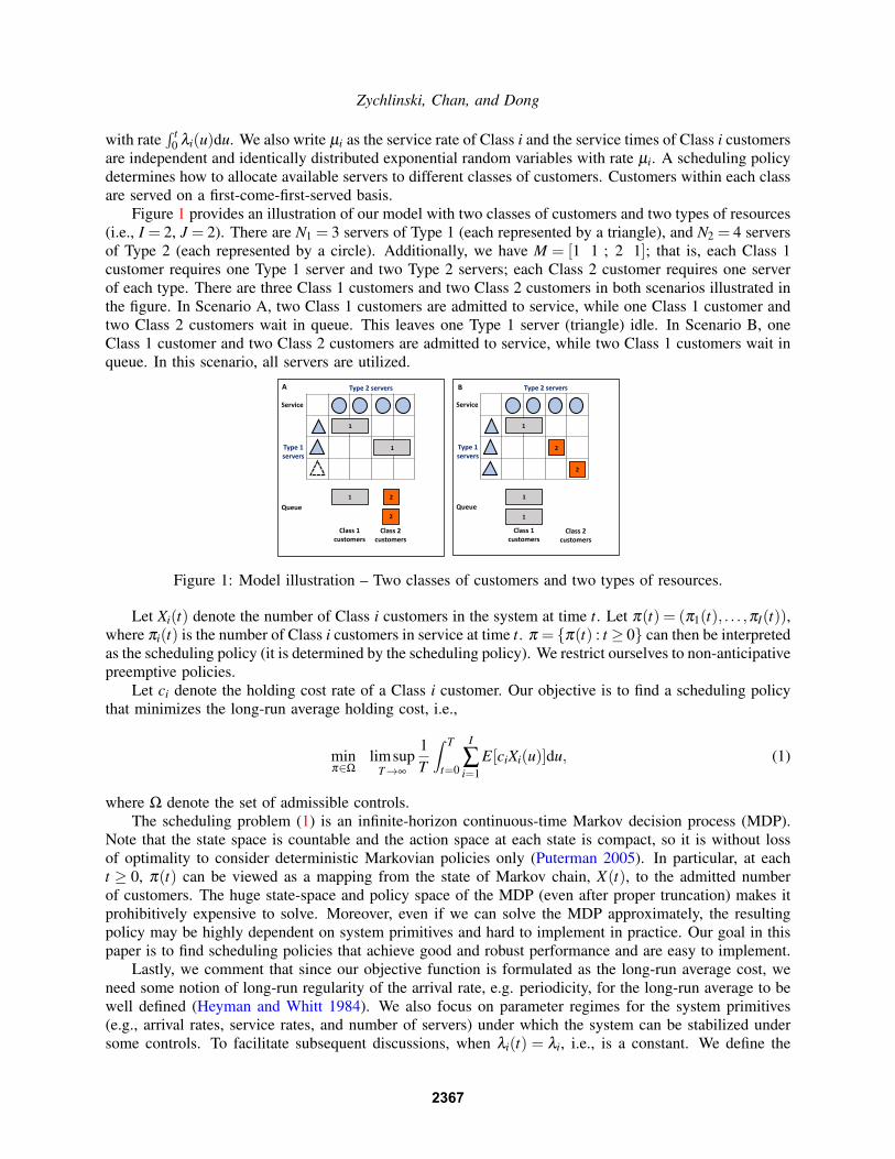
Figure 1 provides an illustration of our model with two classes of customers and two types of resources(i.e., I = 2, J = 2). There are N1 = 3 servers of Type 1 (each represented by a triangle), and N2 = 4 serversof Type 2 (each represented by a circle). Additionally, we have M = [1 1 ; 2 1]; that is, each Class 1customer requires one Type 1 server and two Type 2 servers; each Class 2 customer requires one serverof each type. There are three Class 1 customers and two Class 2 customers in both scenarios illustrated inthe figure. In Scenario A, two Class 1 customers are admitted to service, while one Class 1 customer andtwo Class 2 customers wait in queue. This leaves one Type 1 server (triangle) idle. In Scenario B, oneClass 1 customer and two Class 2 customers are admitted to service, while two Class 1 customers wait inqueue. In this scenario, all servers are utilized.

Figure 1: Model illustration – Two classes of customers and two types of resources.

Let Xi(t) denote the number of Class i customers in the system at time t. Let π(t) = (π1(t), . . . ,πI(t)),where πi(t) is the number of Class i customers in service at time t. π = π(t) : t ≥ 0 can then be interpretedas the scheduling policy (it is determined by the scheduling policy). We restrict ourselves to non-anticipativepreemptive policies.

Let ci denote the holding cost rate of a Class i customer. Our objective is to find a scheduling policythat minimizes the long-run average holding cost, i.e.,

minπ∈Ω

limsupT→∞

1T

∫ T

t=0

I

∑i=1

E[ciXi(u)]du, (1)

where Ω denote the set of admissible controls.The scheduling problem (1) is an infinite-horizon continuous-time Markov decision process (MDP).

Note that the state space is countable and the action space at each state is compact, so it is without lossof optimality to consider deterministic Markovian policies only (Puterman 2005). In particular, at eacht ≥ 0, π(t) can be viewed as a mapping from the state of Markov chain, X(t), to the admitted numberof customers. The huge state-space and policy space of the MDP (even after proper truncation) makes itprohibitively expensive to solve. Moreover, even if we can solve the MDP approximately, the resultingpolicy may be highly dependent on system primitives and hard to implement in practice. Our goal in thispaper is to find scheduling policies that achieve good and robust performance and are easy to implement.

Lastly, we comment that since our objective function is formulated as the long-run average cost, weneed some notion of long-run regularity of the arrival rate, e.g. periodicity, for the long-run average to bewell defined (Heyman and Whitt 1984). We also focus on parameter regimes for the system primitives(e.g., arrival rates, service rates, and number of servers) under which the system can be stabilized undersome controls. To facilitate subsequent discussions, when λi(t) = λi, i.e., is a constant. We define the

2367

Zychlinski, Chan, and Dong

traffic intensity of the system, ρ , as

minρ

s.t.K

∑k=1

αkφk(i)µi = λi for i = 1 . . . , I;K

∑k=1

αk ≤ ρ;

ρ ≥ 0, αk ≥ 0 for k = 1, . . .K,

(2)

where φk = (φk(1), . . . ,φk(I)) denote the k-th possible service configuration, i.e., φk(i) is the number ofClass i customers admitted into service under configuration k. In particular, ρ can be considered as ameasure of the ‘network’ load (Gurvich and Van Mieghem 2015). As will be seen in Section 3.2, withρ < 1, the system is stabilizable.

3 MANAGING IDLENESS

As can be seen from Figure 1, different scheduling rules can induce different levels of idleness (e.g.,Scenario A versus Scenario B). When the system is critically loaded (ρ close to 1), it is important toproperly manage the policy-induced idleness.

A natural way to avoid policy-induced idleness is to add a penalty term to the amount of incurredidleness when evaluating a scheduling rule. For example, Zychlinski et al. (2020) propose a schedulingpolicy that balances the cµ-index and the idleness incurred through an integer program (IP). We can easilyadapt their idea to our setting. In particular, define

maxz

I

∑i=1

ciµizi +Γ(0)

J

∑j=1

I

∑i=1

M jizi

s.t. Mz≤ N

0≤ z≤ x, zi ∈ N, i = 1, . . . , I,

(3)

where Γ(0) ≥ 0 is a hyper parameter for idle-awareness, i.e., by maximizing the objective function in (3),we try to utilize as many servers as possible. We denote by G0 the mapping from x to the optimal z definedby the IP (3). Then, the corresponding scheduling policy sets π(t) = G0(X(t)). We refer to this policy asthe naive idle-aware cµ-rule.

We next use simulation to evaluate the performance of this policy and other benchmark policies. Inthe next and subsequent simulation studies, we plot how the average number of customers in the systemevolves over time for systems starting from some pre-specified initial state. This provides a good amount ofdetails on the system dynamics, including stability. In these experiments, the average number of customersin the system is estimated based on 20 independent replications. Different systems with different primitivesare used in different examples. We provide more details about the system parameters in the caption of thefigures. When the system is stable, we also compare the long-run average costs under different policies insome experiments. These long-run average are estimated using long-time average for T = 6×103.

We next demonstrate the performance of G0 through a simple numerical example. Consider a systemwith N = (3,3) and M = [1 1 ; 1 3]. Figure 2 illustrates the four possible service configurations in thissystem (in addition to the trivial configuration under which no customer is admitted to service). Figure3 shows the average number of customers in the system as a function of time. In addition to the naiveidle-aware cµ-rule, we also consider the classic cµ-rule where we prioritize the class with a larger ciµiindex, and SNOS (smallest number of servers first). SNOS was proposed in Green (1981) for a single-typeof servers. In our case, we adjust it to prioritize customers that require the smallest number of servers intotal (i.e., Class 2 in this example). We observe that the classic cµ-rule, the naive idle-aware cµ-rule, andSNOS all fail to stabilize the system, while this particular system can be stabilized. In particular, underthe system primitives in Figure 3, the traffic intensity defined in (2) is strictly less than 1.

2368

Zychlinski, Chan, and Dong

Figure 2: Possible service configurations when N = (3,3) and M = [1 1 ; 1 3]. The white dashed lineresources represent the idle servers.

0 1000 2000 3000 4000 5000 6000 7000 8000

t

101

102

103

Tota

l avera

ge n

um

ber

of custo

mers

c

Naive Idle-aware c , (0)=100

SNOS

Figure 3: The average number of customers (two classes combined) in the system as a function of timeover a finite horizon T = 8× 103, under different scheduling policies. (N = (3,3), M = [1 1 ; 1 3],µ = (0.34,0.8), λ = (0.25,0.45), c = (1,0.5), x(0) = (5,2).)

3.1 Different Types of Idleness

The observation from Figure 3, which we also see in many other examples, motivates us to look closelyinto the different types of idleness. Specifically, we distinguish between two types of idleness: avoidableidleness and unavoidable idleness.Definition 1 Unavoidable Idleness: A service configuration induces unavoidable idleness if it is infeasibleto admit more customers to service, even though there are idle servers.Definition 2 Avoidable Idleness: A service configuration induces avoidable idleness if at least one additionalcustomer could be admitted to service if there were such customers waiting in the queue.

Configuration A in Figure 2 includes unavoidable idleness: even though two servers of Type 1 areidling, no other customers can be admitted into service. Configurations B and C induce avoidable idleness:if there were more Class 2 customers in the system, they could have been admitted. In Configuration Dthere is no idleness of any type. Note that in this example, even though serving Class 1 customers incursunavoidable idleness of two servers, Configuration A has to be used in order to serve Class 1 customers.On the other hand, it is possible to serve Class 2 customers according to Configuration D, without inducingany amount of idleness. Thus, under a reasonable policy, even though Configuration A and ConfigurationC have the same amount of idle servers, Configuration A should be preferred to Configuration C. Thissuggests that the two types of idleness need to be managed differently.

2369

Zychlinski, Chan, and Dong

3.2 The Generalized Idle-aware (GIA) cµ Rule

Based on the definition of the two types of idleness, we next introduce a modification to the naive idle-awarecµ-rule where we allow different penalties for the two different types of idleness.

We first define the following IP max-min problem:

maxz

minv

R(z,v) :=I

∑i=1

ciµizi−Γ1

J

∑j=1

I

∑i=1

M jivi−Γ2

J

∑j=1

u j

s.t. M(z+ v)+u = N

0≤ z≤ x, zi,vi,ui ∈ N, i = 1, . . . , I,

(4)

where Γ1,Γ2 > 0, are hyper parameters for idle-awareness. To understand the intuition behind (4), wenote that v = (v1, . . . ,vI) can be interpreted as virtual customers. The inner minimization problem tendsto push v to be as large as possible. Thus, the resulting Mv quantifies the amount of avoidable idleness.Meanwhile, from the first constraint, after sending v to its maximum possible value, u quantifies the amountof unavoidable idleness. By introducing two different tuning parameters, Γ1 and Γ2, we can put differentweight on the two types of idleness. Let G denote the mapping from state x to the optimal z defined in(4). Our proposed policy sets π(t) = G(X(t)). We refer to this new policy as the Generalized Idle-Aware(GIA) cµ-rule.

To implement the policy, (4) only needs to be solved at event times (arrival or departure epochs).Solving (4) has limited computational burdens in most settings. We would first try to prioritize the classesaccording to their cµ-index. In the ‘boundary’ states where we incur some idleness after admitting jobsaccording to the cµ-index, we can try swapping some of the admitted jobs with waiting jobs of otherclasses to reduce idleness. In general, if we have enough servers to admit all the jobs or if we have enoughhigh index jobs to fill up all the servers, the solution would be straightforward. We only need to solve (4)in the ‘boundary’ cases. In addition, the IP for these states can be solved off-line and stored. Then, weonly need to look up the solution whenever encountering these states.

In the next section, we study the performance GIA cµ rule with different values of Γ1 and Γ2 usingsimulation. As a quick preview, the left plot in Figure 5 consider the same system as in Figure 3. Weobserve that opposed to the cµ rule and the naive idle-aware cµ rule, the GIA cµ rule with Γ1 = 10 andΓ2 = 1 stabilizes the system with an estimated long-run average cost of 10.

4 IDLE-AWARE PARAMETERS

The GIA cµ-rule is a very flexible class of policies. Note that if Γ1 = Γ2 = 0, we retrieve the cµ-rule, andwhen Γ1 = Γ2, we retrieve the naive idle-aware cµ-rule. As was shown in Figure 3, both policies can leadto poor performances due to instability. Thus, it is important to set some basic rules as how to choose theidle-aware parameters.

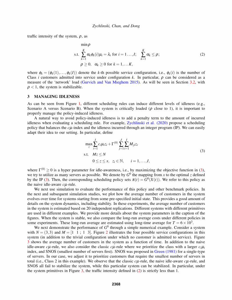
Our first rule is that both parameters need to be positive, i.e., both types idleness need to be managed.To see this, we consider two different models. The first one is the one shown in Figure 2. The second oneis illustrated in Figure 4. Note that both Configurations A and B in Figure 4 do not incur any avoidableidleness. However, Configuration A incurs less unavoidable idleness than Configuration B. Figure 5 showsthe average number of customers in the system as a function of time in the two models (left versus right)under the GIA cµ-rule with different values of (Γ1,Γ2). We observe that in the left plot, having Γ1 = 0leads to instability. That is because when Γ1 = 0, under the system parameters, Configurations B, C, andD are preferred to Configuration A in Figure 2. In other words, Class 1 customers are served only whenthere are no Class 2 customers in the system. The Class 1 queue blows up in this case as we incur toomuch avoidable idleness when implementing Configurations B and C. In the right plot we see that Γ2 = 0can lead to instability. This is because when Γ2 = 0, under the system parameters, Configuration B ispreferred to Configuration A in Figure 4. In this case, we end up serving the Class 2 queue too fast that

2370

Zychlinski, Chan, and Dong

when we switch to serve the Class 1 queue, there is no Class 2 customer left, i.e., we can serve only oneClass 1 customer while incurring two units of avoidable idleness. Thus, even though the Class 2 queue ismaintained close to zero, the Class 1 queue blows up.

Figure 5 also shows that Γ1 needs to be larger than Γ2; i.e., we should put more penalty (weight) onavoidable idleness than unavoidable idleness. Thus, our second rule is that Γ1 should be larger than Γ2,i.e., it is more important to reduce avoidable idleness.

Our third rule is that both Γ1 and Γ2 need to be sufficiently large. To see this, in Figure 6, we comparethe average number of customers as a function of time for the two models (left versus right) under the GIAcµ-rule with different values of (Γ1,Γ2) satisfying Γ1 Γ2. We use a periodic time-varying arrival ratein this figure. We observe that having Γ1 Γ2 > 0 alone may not be enough. Both Γ1 and Γ2 need besufficiently large, i.e., we need to put enough weight on both types of idleness, to ensure system stability.

To sum up, we note that the “appropriate” values of (Γ1,Γ2) can be highly dependent on systemparameters, i.e., c, µ , N and M. For example, setting Γ1 = 1 and Γ2 = 0.1 stabilizes the system in theleft plot of Figure 6, but fails to stabilize the system in the right plot of that figure. We next take a closerlook at the two examples in Figure 6. In the left plot (for the system depicted in Figure 2), it is importantto make sure that Γ1 is large enough so that Configuration A is preferred to Configurations B and C (i.e.eliminate the avoidable idleness). In the right plot (for the system depicted in Figure 4), it is important tomake sure that Γ2 is large enough so that Configuration A is preferred to Configuration B (i.e. eliminatethe unavoidable idleness). More generally, from the perspective of throughput optimality, we need to makesure that Γ1 and Γ2 are chosen such that we put a higher weight on minimizing the idleness than maximizingthe cµ index. In particular, Γ1 should be larger than max1≤i≤I ciµisi, where si = min1≤ j≤J N( j)/M( j, i) isthe maximal number of Class i customers allowed in service. We can then fine-tune the value of Γ2 to putenough weight on unavoidable idleness.

Figure 4: Service configuration for N = (2,4) and M = [1 1 ; 1 3].

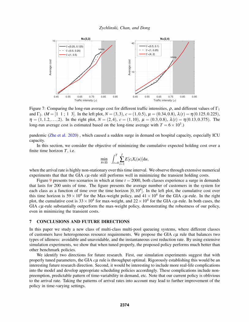
When taking cost minimization into account, the optimal choice of (Γ1,Γ2) may depend on the loadof the system. The general rule of thumb is that when the system is lightly loaded, we should put moreweight on the instantaneous cost-reduction rate, i.e., the ciµi’s, as managing idleness is of less concern.When the system is heavily loaded, we should put more weight on the two types of idleness. For example,in Figure 7 we compare the long-run average costs of the two models (left versus right) with differenttraffic intensities (defined in (2)) under the GIA cµ rule with different values of (Γ1,Γ2). We observe thatwhen traffic intensity is low, policies with different hyper-parameters perform similarly. Indeed, when ρ issufficiently small, the GIA cµ rule with smaller values (Γ1,Γ2) performs slightly better than that with thatwith large values of (Γ1,Γ2), e.g., when ρ < 0.7 in the right plot, (Γ1,Γ2) = (0.5,0.25) or (1,0.25) areperforming better than (Γ1,Γ2) = (4,2). However, as traffic intensity grows, the larger values of (Γ1,Γ2)lead to better performance. Note that when ρ is large (gray area in the plots), the GIA cµ rule with smallvalues of (Γ1,Γ2) can not stabilize the system. To set a general rule of thumb, we note that when ρ is small,the performances of GIA cµ rule is similar for different values of (Γ1,Γ2). When ρ is large, however,large values of (Γ1,Γ2) perform substantially better. Thus, we suggest to first set Γ1 to be larger thanmax1≤i≤I ciµisi, where si = min1≤ j≤J N( j)/M( j, i); then to set Γ2 to be a positive number that is smallerthan Γ1.

2371

Zychlinski, Chan, and Dong

0 1000 2000 3000 4000 5000

t

101

102

To

tal a

ve

rag

e n

um

be

r o

f cu

sto

me

rs

N=(3,3)

=(0,10)

=(10,0)

=(1,10)

=(10,1)

0 1000 2000 3000 4000 5000

t

101

102

To

tal a

ve

rag

e n

um

be

r o

f cu

sto

me

rs

N=(2,4)

=(0,10)

=(10,0)

=(1,10)

=(10,1)

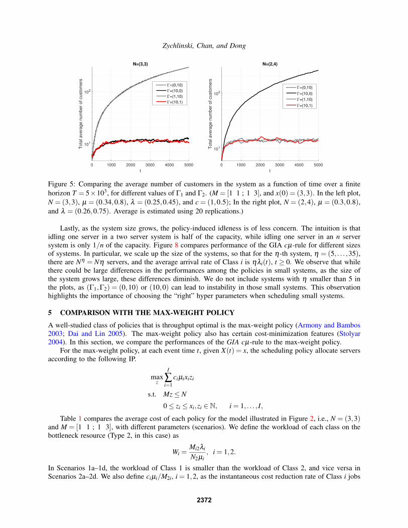
Figure 5: Comparing the average number of customers in the system as a function of time over a finitehorizon T = 5×103, for different values of Γ1 and Γ2. (M = [1 1 ; 1 3], and x(0) = (3,3). In the left plot,N = (3,3), µ = (0.34,0.8), λ = (0.25,0.45), and c = (1,0.5); In the right plot, N = (2,4), µ = (0.3,0.8),and λ = (0.26,0.75). Average is estimated using 20 replications.)

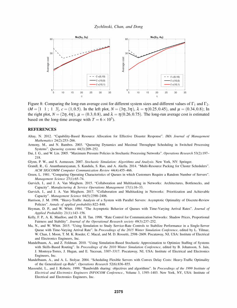
Lastly, as the system size grows, the policy-induced idleness is of less concern. The intuition is thatidling one server in a two server system is half of the capacity, while idling one server in an n serversystem is only 1/n of the capacity. Figure 8 compares performance of the GIA cµ-rule for different sizesof systems. In particular, we scale up the size of the systems, so that for the η-th system, η = (5, . . . ,35),there are Nη = Nη servers, and the average arrival rate of Class i is ηλi(t), t ≥ 0. We observe that whilethere could be large differences in the performances among the policies in small systems, as the size ofthe system grows large, these differences diminish. We do not include systems with η smaller than 5 inthe plots, as (Γ1,Γ2) = (0,10) or (10,0) can lead to instability in those small systems. This observationhighlights the importance of choosing the “right” hyper parameters when scheduling small systems.

5 COMPARISON WITH THE MAX-WEIGHT POLICY

A well-studied class of policies that is throughput optimal is the max-weight policy (Armony and Bambos2003; Dai and Lin 2005). The max-weight policy also has certain cost-minimization features (Stolyar2004). In this section, we compare the performances of the GIA cµ-rule to the max-weight policy.

For the max-weight policy, at each event time t, given X(t) = x, the scheduling policy allocate serversaccording to the following IP.

maxz

I

∑i=1

ciµixizi

s.t. Mz≤ N

0≤ zi ≤ xi,zi ∈ N, i = 1, . . . , I,

Table 1 compares the average cost of each policy for the model illustrated in Figure 2, i.e., N = (3,3)and M = [1 1 ; 1 3], with different parameters (scenarios). We define the workload of each class on thebottleneck resource (Type 2, in this case) as

Wi =Mi2λi

N2µi, i = 1,2.

In Scenarios 1a–1d, the workload of Class 1 is smaller than the workload of Class 2, and vice versa inScenarios 2a–2d. We also define ciµi/M2i, i = 1,2, as the instantaneous cost reduction rate of Class i jobs

2372

Zychlinski, Chan, and Dong

0 1000 2000 3000 4000 5000

t

0

50

100

150

200

250

300

To

tal n

um

be

r o

f cu

sto

me

rs

N=(3,3)

=(0.02, 0.01)

=(0.5, 0.05)

=(1, 0.1)

=(5, 0.5)

0 1000 2000 3000 4000 5000

t

0

50

100

150

200

250

300

Tota

l avera

ge n

um

ber

of custo

mers

N=(2,4)

=(0.02, 0.01)

=(0.5, 0.05)

=(1, 0.1)

=(5, 0.5)

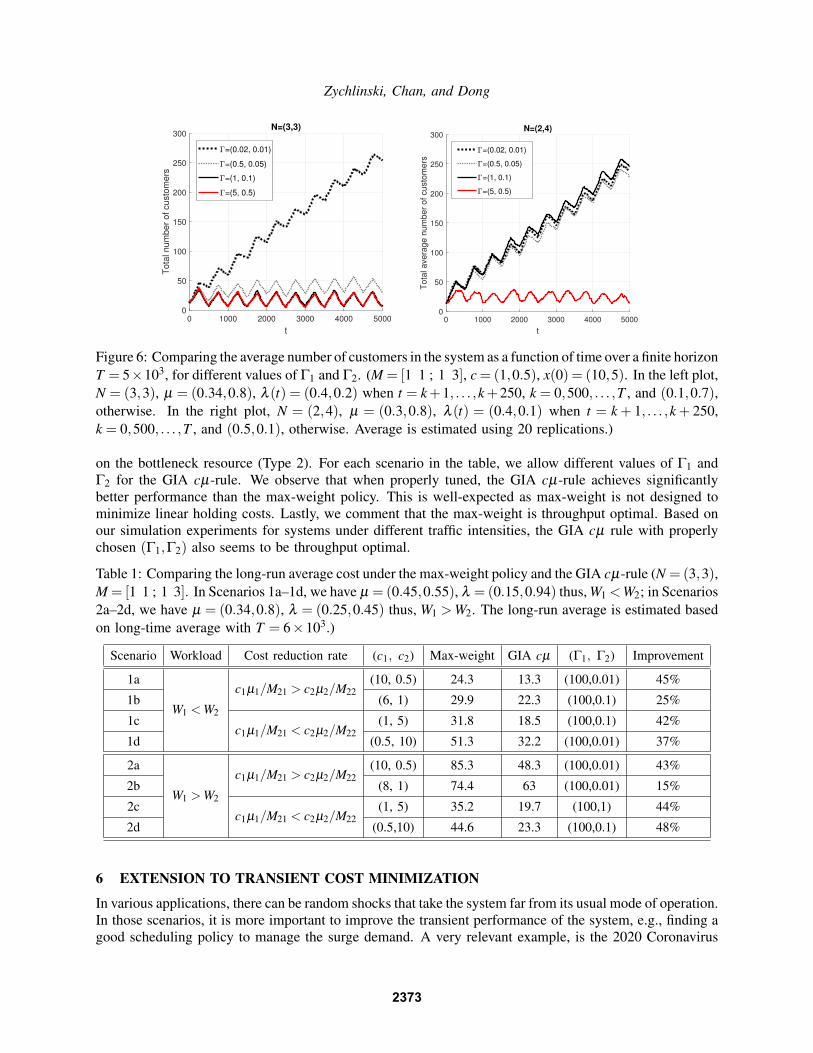
Figure 6: Comparing the average number of customers in the system as a function of time over a finite horizonT = 5×103, for different values of Γ1 and Γ2. (M = [1 1 ; 1 3], c = (1,0.5), x(0) = (10,5). In the left plot,N = (3,3), µ = (0.34,0.8), λ (t) = (0.4,0.2) when t = k+1, . . . ,k+250, k = 0,500, . . . ,T , and (0.1,0.7),otherwise. In the right plot, N = (2,4), µ = (0.3,0.8), λ (t) = (0.4,0.1) when t = k + 1, . . . ,k + 250,k = 0,500, . . . ,T , and (0.5,0.1), otherwise. Average is estimated using 20 replications.)

on the bottleneck resource (Type 2). For each scenario in the table, we allow different values of Γ1 andΓ2 for the GIA cµ-rule. We observe that when properly tuned, the GIA cµ-rule achieves significantlybetter performance than the max-weight policy. This is well-expected as max-weight is not designed tominimize linear holding costs. Lastly, we comment that the max-weight is throughput optimal. Based onour simulation experiments for systems under different traffic intensities, the GIA cµ rule with properlychosen (Γ1,Γ2) also seems to be throughput optimal.

Table 1: Comparing the long-run average cost under the max-weight policy and the GIA cµ-rule (N = (3,3),M = [1 1 ; 1 3]. In Scenarios 1a–1d, we have µ = (0.45,0.55), λ = (0.15,0.94) thus, W1 <W2; in Scenarios2a–2d, we have µ = (0.34,0.8), λ = (0.25,0.45) thus, W1 >W2. The long-run average is estimated basedon long-time average with T = 6×103.)

Scenario Workload Cost reduction rate (c1, c2) Max-weight GIA cµ (Γ1, Γ2) Improvement

1a

W1 <W2

c1µ1/M21 > c2µ2/M22(10, 0.5) 24.3 13.3 (100,0.01) 45%

1b (6, 1) 29.9 22.3 (100,0.1) 25%

1cc1µ1/M21 < c2µ2/M22

(1, 5) 31.8 18.5 (100,0.1) 42%

1d (0.5, 10) 51.3 32.2 (100,0.01) 37%

2a

W1 >W2

c1µ1/M21 > c2µ2/M22(10, 0.5) 85.3 48.3 (100,0.01) 43%

2b (8, 1) 74.4 63 (100,0.01) 15%

2cc1µ1/M21 < c2µ2/M22

(1, 5) 35.2 19.7 (100,1) 44%

2d (0.5,10) 44.6 23.3 (100,0.1) 48%

6 EXTENSION TO TRANSIENT COST MINIMIZATION

In various applications, there can be random shocks that take the system far from its usual mode of operation.In those scenarios, it is more important to improve the transient performance of the system, e.g., finding agood scheduling policy to manage the surge demand. A very relevant example, is the 2020 Coronavirus

2373

Zychlinski, Chan, and Dong

N=(3,3)

0.45 0.55 0.65 0.75 0.85 0.95

Traffic intensity ( )

10

Avera

ge c

ost

=(0.25, 0.125)

=(0.5, 0.25)

=(1, 0.5)

Infinity

N=(2,4)

0.45 0.55 0.65 0.75 0.85 0.95

Traffic intensity ( )

10

40

Avera

ge c

ost

=(0.5, 0.1)

=(1, 0.25)

=(4, 2)

Infinity

Figure 7: Comparing the long-run average cost for different traffic intensities, ρ , and different values of Γ1and Γ2. (M = [1 1 ; 1 3]. In the left plot, N = (3,3), c = (1,0.5), µ = (0.34,0.8), λ (t) = η(0.125,0.225),η = (1,1.2, . . . ,2). In the right plot, N = (2,4), c = (1,10), µ = (0.3,0.8), λ (t) = η(0.13,0.375). Thelong-run average cost is estimated based on the long-time average with T = 6×103.)

pandemic (Zhe et al. 2020) , which caused a sudden surge in demand on hospital capacity, especially ICUcapacity.

In this section, we consider the objective of minimizing the cumulative expected holding cost over afinite time horizon T , i.e.

minπ∈Ω

∫ T

t=0

I

∑i=1

E[ciXi(u)]du,

when the arrival rate is highly non-stationary over this time interval. We observe through extensive numericalexperiments that that the GIA cµ-rule still performs well in minimizing the transient holding costs.

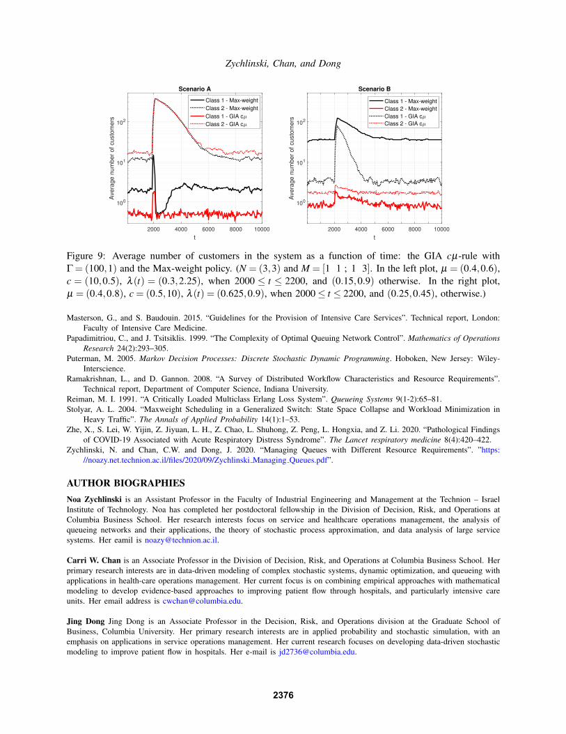
Figure 9 presents two scenarios in which at time t = 2000, both classes experience a surge in demandsthat lasts for 200 units of time. The figure presents the average number of customers in the system foreach class as a function of time over the time horizon [0,104]. In the left plot, the cumulative cost overthis time horizon is 59×104 for the Max-weight policy, and 41×104 for the GIA cµ-rule. In the rightplot, the cumulative cost is 33×104 for max-weight, and 22×104 for the GIA cµ-rule. In both cases, theGIA cµ-rule substantially outperform the max-weight policy, demonstrating the robustness of our policy,even in minimizing the transient costs.

7 CONCLUSIONS AND FUTURE DIRECTIONS

In this paper we study a new class of multi-class multi-pool queueing systems, where different classesof customers have heterogeneous resource requirements. We propose the GIA cµ rule that balances twotypes of idleness: avoidable and unavoidable, and the instantaneous cost reduction rate. By using extensivesimulation experiments, we show that when tuned properly, the proposed policy performs much better thanother benchmark policies.

We identify two directions for future research. First, our simulation experiments suggest that withproperly tuned parameters, the GIA cµ rule is throughput optimal. Rigorously establishing this would be aninteresting future research direction. Second, it would be interesting to include more real-life complicationsinto the model and develop appropriate scheduling policies accordingly. These complications include non-preemption, predictable pattern of time-variability in demand, etc. Note that our current policy is obliviousto the arrival rate. Taking the patterns of arrival rates into account may lead to further improvement of thepolicy in time-varying settings.

2374

Zychlinski, Chan, and Dong

5 10 15 20 25 30 355

30

60

Avera

ge c

ost

N=(3 , 3 )

=(0,10)

=(10,0)

=(10,1)

5 10 15 20 25 30 355

30

60

Avera

ge c

ost

N=(2 , 4 )

=(0,10)

=(10,0)

=(10,1)

Figure 8: Comparing the long-run average cost for different system sizes and different values of Γ1 and Γ2.(M = [1 1 ; 1 3], c = (1,0.5). In the left plot, N = (3η ,3η), λ = η(0.25,0.45), and µ = (0.34,0.8); Inthe right plot, N = (2η ,4η), µ = (0.3,0.8), and λ = η(0.26,0.75). The long-run average cost is estimatedbased on the long-time average with T = 6×103).

REFERENCESAltay, N. 2012. “Capability-Based Resource Allocation for Effective Disaster Response”. IMA Journal of Management

Mathematics 24(2):253–266.Armony, M., and N. Bambos. 2003. “Queueing Dynamics and Maximal Throughput Scheduling in Switched Processing

Systems”. Queueing systems 44(3):209–252.Dai, J. G., and W. Lin. 2005. “Maximum Pressure Policies in Stochastic Processing Networks”. Operations Research 53(2):197–

218.Glynn, P. W., and S. Asmussen. 2007. Stochastic Simulation: Algorithms and Analysis. New York, NY: Springer.Grandl, R., G. Ananthanarayanan, S. Kandula, S. Rao, and A. Akella. 2014. “Multi-Resource Packing for Cluster Schedulers”.

ACM SIGCOMM Computer Communication Review 44(4):455–466.Green, L. 1981. “Comparing Operating Characteristics of Queues in which Customers Require a Random Number of Servers”.

Management Science 27(1):65–74.Gurvich, I., and J. A. Van Mieghem. 2015. “Collaboration and Multitasking in Networks: Architectures, Bottlenecks, and

Capacity”. Manufacturing & Service Operations Management 17(1):16–33.Gurvich, I., and J. A. Van Mieghem. 2017. “Collaboration and Multitasking in Networks: Prioritization and Achievable

Capacity”. Management Science 64(5):2390–2406.Harrison, J. M. 1998. “Heavy-Traffic Analysis of a System with Parallel Servers: Asymptotic Optimality of Discrete-Review

Policies”. Annals of applied probability:822–848.Heyman, D. P., and W. Whitt. 1984. “The Asymptotic Behavior of Queues with Time-Varying Arrival Rates”. Journal of

Applied Probability 21(1):143–156.Kelly, F. P., A. K. Maulloo, and D. K. H. Tan. 1998. “Rate Control for Communication Networks: Shadow Prices, Proportional

Fairness and Stability”. Journal of the Operational Research society 49(3):237–252.Ma, N., and W. Whitt. 2015. “Using Simulation to Study Service-Rate Controls to Stabilize Performance in a Single-Server

Queue with Time-Varying Arrival Rate”. In Proceedings of the 2015 Winter Simulation Conference, edited by L. Yilmaz,W. Chan, I. Moon, T. M. K. Roeder, C. Macal, and M. D. Rossetti, 2598–2609. Piscataway, NJ, USA: Institute of Electricaland Electronics Engineers, Inc.

Mandelbaum, A., and Z. Feldman. 2010. “Using Simulation-Based Stochastic Approximation to Optimize Staffing of Systemswith Skills-Based Routing”. In Proceedings of the 2010 Winter Simulation Conference, edited by B. Johansson, S. Jain,J. Montoya-Torres, J. Hugan, and E. Yucesan, 3307–3317. Piscataway, NJ, USA: Institute of Electrical and ElectronicsEngineers, Inc.

Mandelbaum, A., and A. L. Stolyar. 2004. “Scheduling Flexible Servers with Convex Delay Costs: Heavy-Traffic Optimalityof the Generalized cµ-Rule”. Operations Research 52(6):836–855.

Massoulie, L., and J. Roberts. 1999. “Bandwidth sharing: objectives and algorithms”. In Proceedings of the 1999 Institute ofElectrical and Electronics Engineers INFOCOM Conference., Volume 3, 1395–1403. New York, NY, USA: Institute ofElectrical and Electronics Engineers, Inc.

2375

Zychlinski, Chan, and Dong

2000 4000 6000 8000 10000

t

100

101

102

Ave

rag

e n

um

be

r o

f cu

sto

me

rs

Scenario A

Class 1 - Max-weight

Class 2 - Max-weight

Class 1 - GIA c

Class 2 - GIA c

2000 4000 6000 8000 10000

t

100

101

102

Ave

rag

e n

um

be

r o

f cu

sto

me

rs

Scenario B

Class 1 - Max-weight

Class 2 - Max-weight

Class 1 - GIA c

Class 2 - GIA c

Figure 9: Average number of customers in the system as a function of time: the GIA cµ-rule withΓ = (100,1) and the Max-weight policy. (N = (3,3) and M = [1 1 ; 1 3]. In the left plot, µ = (0.4,0.6),c = (10,0.5), λ (t) = (0.3,2.25), when 2000 ≤ t ≤ 2200, and (0.15,0.9) otherwise. In the right plot,µ = (0.4,0.8), c = (0.5,10), λ (t) = (0.625,0.9), when 2000≤ t ≤ 2200, and (0.25,0.45), otherwise.)

Masterson, G., and S. Baudouin. 2015. “Guidelines for the Provision of Intensive Care Services”. Technical report, London:Faculty of Intensive Care Medicine.

Papadimitriou, C., and J. Tsitsiklis. 1999. “The Complexity of Optimal Queuing Network Control”. Mathematics of OperationsResearch 24(2):293–305.

Puterman, M. 2005. Markov Decision Processes: Discrete Stochastic Dynamic Programming. Hoboken, New Jersey: Wiley-Interscience.

Ramakrishnan, L., and D. Gannon. 2008. “A Survey of Distributed Workflow Characteristics and Resource Requirements”.Technical report, Department of Computer Science, Indiana University.

Reiman, M. I. 1991. “A Critically Loaded Multiclass Erlang Loss System”. Queueing Systems 9(1-2):65–81.Stolyar, A. L. 2004. “Maxweight Scheduling in a Generalized Switch: State Space Collapse and Workload Minimization in

Heavy Traffic”. The Annals of Applied Probability 14(1):1–53.Zhe, X., S. Lei, W. Yijin, Z. Jiyuan, L. H., Z. Chao, L. Shuhong, Z. Peng, L. Hongxia, and Z. Li. 2020. “Pathological Findings

of COVID-19 Associated with Acute Respiratory Distress Syndrome”. The Lancet respiratory medicine 8(4):420–422.Zychlinski, N. and Chan, C.W. and Dong, J. 2020. “Managing Queues with Different Resource Requirements”. ”https:

//noazy.net.technion.ac.il/files/2020/09/Zychlinski Managing Queues.pdf”.

AUTHOR BIOGRAPHIESNoa Zychlinski is an Assistant Professor in the Faculty of Industrial Engineering and Management at the Technion – IsraelInstitute of Technology. Noa has completed her postdoctoral fellowship in the Division of Decision, Risk, and Operations atColumbia Business School. Her research interests focus on service and healthcare operations management, the analysis ofqueueing networks and their applications, the theory of stochastic process approximation, and data analysis of large servicesystems. Her eamil is noazy@technion.ac.il.

Carri W. Chan is an Associate Professor in the Division of Decision, Risk, and Operations at Columbia Business School. Herprimary research interests are in data-driven modeling of complex stochastic systems, dynamic optimization, and queueing withapplications in health-care operations management. Her current focus is on combining empirical approaches with mathematicalmodeling to develop evidence-based approaches to improving patient flow through hospitals, and particularly intensive careunits. Her email address is cwchan@columbia.edu.

Jing Dong Jing Dong is an Associate Professor in the Decision, Risk, and Operations division at the Graduate School ofBusiness, Columbia University. Her primary research interests are in applied probability and stochastic simulation, with anemphasis on applications in service operations management. Her current research focuses on developing data-driven stochasticmodeling to improve patient flow in hospitals. Her e-mail is jd2736@columbia.edu.

2376