July 2010 RFF DP 10-37 DISCUSSION PAPER Mine K. Y¼cel

1616 P St. NW Washington, DC 20036 202-328-5000 www.rff.org

July 2010 RFF DP 10-37

Oil Price Shocks and U.S. Economic Activity

An International Perspective

Nathan S . Ba lke , S tephen P .A . Bro w n , and

M ine K . Yüce l

DIS

CU

SSIO

N P

APE

R

© 2010 Resources for the Future. All rights reserved. No portion of this paper may be reproduced without permission of the authors.

Discussion papers are research materials circulated by their authors for purposes of information and discussion. They have not necessarily undergone formal peer review.

Oil Price Shocks and U.S. Economic Activity: An International Perspective

Nathan S. Balke, Stephen P.A. Brown and Mine K. Yücel

Abstract Oil price shocks are thought to have played a prominent role in U.S. economic activity. In this

paper, we employ Bayesian methods with a dynamic stochastic general equilibrium model of world economic activity to identify the various sources of oil price shocks and economic fluctuation and to assess their effects on U.S. economic activity. We find that changes in oil prices are best understood as endogenous. Oil price shocks in the 1970s and early 1980s and the 2000s reflect differing mixes of shifts in oil supply and demand, and differing sources of oil price shocks have differing effects on economic activity. We also find that U.S. output fluctuations owe mostly to domestic shocks, with productivity shocks contributing to weakness in the 1970s and 1980s and strength in the 2000s.

Key Words: oil price, international business cycles, general equilibrium, Bayesian estimation

JEL Classification Numbers: C3, E3, Q43

Contents

1. Introduction ......................................................................................................................... 1

2. The Model ............................................................................................................................ 3

2.1 Consumers..................................................................................................................... 4

2.2 Manufacturing, Production, and Investment ................................................................. 5

2.3 Oil Production and Reserves ......................................................................................... 6

2.4 International Market Clearing Constraints .................................................................... 8

3. Model Estimation ................................................................................................................ 8

3.1 Prior and Posterior Distributions of the Structural Parameters ..................................... 9

4. Estimated Impulse Responses .......................................................................................... 11

4.1 Responses of the Oil Market to Structural Shocks ..................................................... 12

4.2 Oil Supply Shocks and U.S. Economic Activity ........................................................ 13

5. Historical Decompositions ................................................................................................ 14

5.1 Real Oil Price and Oil Output ..................................................................................... 15

5.2 U.S. Economic Activity .............................................................................................. 15

5.3 Oil Prices and U.S. Economic Activity in the 1970s to Early 1980s and the 2000s .. 16

5.4 Sources of ROW Fluctuations .................................................................................... 17

6. Model Robustness ............................................................................................................. 17

7. Conclusions ........................................................................................................................ 19

References .............................................................................................................................. 21

Technical Appendix .............................................................................................................. 24

Tables and Figures ................................................................................................................ 28

Resources for the Future Balke, Brown, and Yücel

1

Oil Price Shocks and U.S. Economic Activity: An International Perspective

Nathan S. Balke, Stephen P.A. Brown and Mine K. Yücel∗

1. Introduction

Economic research has long focused on the aggregate economic effects of unfavorable oil supply shocks. Some of the earlier studies examining oil price shocks include Rasche and Tatom (1977), Mork and Hall (1980), Hamilton (1983), and the Energy Modeling Forum 7 study documented by Hickman et al. (1987). As reported in surveys by Brown and Yücel (2002), Jones et al, (2004), and Kilian (2008c), the literature finds such consequences as rising oil prices, slower GDP growth and possible recession, higher unemployment rates, and higher price levels.

As oil prices rose sharply in the 2000s, however, the gains in oil prices seemed to be positively related to economic growth. The apparent weakening or reversal of the past economic effects of oil price shocks stimulated a new literature about why the U.S. economy might respond differently to rising oil prices in the 2000s than it did in the 1970s and early 80s. The explanations include increased global financial integration, greater flexibility of the U.S. economy (including labor and financial markets), the reduced energy intensity of the U.S. economy, increased experience with energy price shocks, better monetary policy, and good luck—that is, smaller and less frequent shocks. Contributions include Huntington (2003), Stock and Watson (2003), Congressional Budget Office (2006), Blanchard and Gali (2007), Edelstein and Kilian (2007), Segal (2007), and Herrera and Pesavento (2009), who mostly treat oil price shocks as exogenous.

In contrast, an emerging literature explores the implications of treating oil price shocks as endogenous with sources that could include demand as well as supply, including Barsky and

∗ Nathan S. Balke is Dedman Family Distinguished Professor at Southern Methodist University and research associate at the Federal Reserve Bank of Dallas. Stephen P.A. Brown is a nonresident fellow at Resources for the Future. Mine K. Yücel is vice president and senior economist at the Federal Reserve Bank of Dallas. The authors thank Roger Cooke, Mario Crucini, Fred Joutz, Luca Guerrieri, William Helkie, Lutz Kilian, Prakash Loungani, Erwan Quintin, Tara Sinclair, Mark Wynne, and Carlos Zarazaga for helpful comments and discussions and Stefan Avdjiev, Xin Jin, and Zheng Zeng for capable research assistance. The authors retain all responsibility for omissions and errors. The views expressed are those of the authors and should not be attributed to the Federal Reserve Bank of Dallas, the Federal Reserve System, Resources for the Future, or Southern Methodist University.


2

Kilian (2002, 2004), Bodenstein et al. (2007), Nakov and Pescatori (2007a, 2007b) and Kilian (2008a, 2008b, 2009). The differing sources of oil price shocks can explain the apparent instability of the relationship between oil prices and aggregate economic activity.

Kilian (2008b) maintains that most of the oil price gains after 1970 were the result of demand shocks; only the recession of 1980–1982 was the result of exogenous oil supply shocks; and exogenous supply shocks explain only a small fraction of the oil price increases during the 1973–1974, 1990–1991, and 2002–2003 episodes. Kilian (2009) identifies oil price shocks as variously arising from shocks to crude oil supply, global demand, and precautionary demand and then uses a vector autoregressive model to show that the different sources of shocks have substantially differential effects on U.S. GDP and consumer prices.

In the present analysis, we attempt to identify the sources and consequences of oil price fluctuations on economic activity. Instead of using a reduced-form vector autoregressive model, we use a dynamic stochastic general equilibrium (DSGE) model of world economic activity. The model provides a mapping from “structural shocks” in technology and preferences to observables such as oil prices, oil output, and other measures of economic activity. Our model is similar to that of Backus and Crucini (2000) in that the world economy is represented as two manufacturing countries and an oil-producing country. The model includes many features in the recent DSGE literature, such as the inclusion of oil in consumption (Bodenstein et al. 2007) and a general specification of preferences (Jaimovich and Rebelo 2009).

Our model departs from the previous literature by treating oil supply decisions in an optimizing framework. Oil producers face an intertemporal trade-off when deciding how much oil to produce: higher production today reduces the oil reserves available in the future. Oil producers can also invest to expand oil reserves, which increases future oil production capacity. Thus, the evolution of reserves and production are choice variables for producers.

Rather than calibrate the parameters of the model and use it for a simulation exercise, we use Bayesian methods to estimate the parameters of technology and preferences as well as the parameters for the stochastic process generating the exogenous shocks. In estimating the parameters, we also estimate realizations for the unobserved shock processes. The latter allows us to identify and differentiate oil supply and demand shocks. In particular, the model allows us to estimate the effects of various types of shocks on oil markets and aggregate economic activity. These shocks include those to oil production and oil reserves in the oil-producing countries, and total factor productivity, preferences between goods and leisure, investment efficiency, and oil efficiency in the manufacturing countries.


3

Over the 1970–2009 period for which the model is estimated, historical decompositions suggest that nearly all the fluctuations in oil prices and oil output are due to oil-specific shocks—either oil supply shocks originating in the oil-producing country or oil efficiency shocks originating in the manufacturing countries. We find oil supply shocks contributed to long swings in oil prices and oil output, while oil efficiency shocks contributed much of the higher frequency movements in oil prices and oil output. Nonetheless, these oil-specific shocks had only mild effects on the growth of U.S. real GDP.

U.S. economic fluctuations are estimated to be due largely to domestic shocks in total factor productivity, preferences for goods versus leisure, and investment. The episodes of poor U.S. economic performance during our 1970–2009 estimation period appear to be mostly the result of negative shocks to total factor productivity and labor supply. Some episodes of weak economic activity were coincident with sharply rising oil prices, and in some cases, unfavorable oil supply shocks contributed to a slight drag on U.S. economic activity

2. The Model

We approach identification of the source of oil price fluctuations through the lens of a three-country DSGE model. The model combines elements from the open economy model of Backus and Crucini (2000) with oil market features in Bodenstein et al. (2007) and the recent generalization of preferences proposed by Jaimovich and Rebelo (2009). Two countries each produce a final manufactured good. The third country produces oil, which is both a consumption good and an intermediate good used in the production of the manufactured goods.

Departing from Backus and Crucini, we treat oil production and the evolution of oil reserves in the oil-producing country as completely endogenous.1 This treatment of oil production and pricing allows us to consider the role that shocks originating in the two manufacturing countries can have in generating oil price fluctuations. By modeling the evolution of oil reserves, we introduce an intertemporal channel through which oil markets can be affected and expectations about future oil prices can have a direct effect on current oil prices.

1 Backus and Crucini (2000) represent oil production as having an exogenous component (Organization of Petroleum Exporting Countries) and an endogenous supply component via a labor-only technology.


4

2.1 Consumers

In each of the three countries, consumers directly use the two manufactured goods and face a labor–leisure trade-off. Accordingly, consumers in each country j maximize lifetime utility:

β tU(C j,t ,N j,t )t= 0

∞

∑ for j = a, b, o, (1)

where β is a discount factor, t,jC is the consumption of the representative agent in country j, and N j ,t is hours worked. We adopt the preference specification proposed by Jaimovich and Rebelo

(2009):

U(C j,t ,L j,t ) =(C j ,t − χN j ,t

η X j,tZ j ,tU )1−σ

1−σ , (2)

where X j,t = Cj,tγ X j,t−1

1−γ , X j,t reflects a time varying disutility of work that depends on past consumption choices, U

t,jZ is a exogenous preference shock, and γ determines the strength of the

wealth effect on the supply of labor. As in Jaimovich and Rebelo, Equation 2 embeds two classes of utility functions widely used in the literature. If γ=1, we have the standard set of preferences as in King et al. (1988). If γ=0, preferences are as in Greenwood et al. (1988), and there is no wealth effect on the supply of labor.

To assess the effect of oil price fluctuations on consumption, we utilize a consumption function that is a CES aggregate of manufactured goods and oil usage as in Bodenstein et al. (2007),

C j,t = [ωGc Gc, j,t

1−μc + (1−ωGc )Z j,t

E Oc, j,t1−μc ]1/(1−μc ) for j = a, b, o, (3)

where Gc,j,t is country j’s use of manufactured goods and Oc,j,t is the country j’s use of oil for consumption, c

gω captures the weight households place on the consumption of goods relative to

oil, cμ is the elasticity of substitution between goods and oil in consumption, and Et,jZ is a

exogenous shock that affects the relative efficiency of oil usage and is common to both production and consumption.2 This specification captures the reality that oil is used in the

2 For the oil-producing country, we drop Z j,t

U , Z j,tE from preferences because we lack the detailed data with which to

separately identify such shocks.


5

consumer sector and is in line with Edelstein and Kilian (2007), who show that consumer spending on energy is a major transmission mechanism of oil price shocks.

Manufactured goods are themselves a composite of domestic and foreign produced goods:

Gc, j ,t = [ωA , jg,c Ac, j,t

1−μg + (1−ωA , jg,c )Bc, j ,t

1−μg ]1/(1−μg )

(4)

where ωA , jg,c

is the weight that good A (produced by country a) receives in country j’s composite consumption good. Assuming home bias, ωA,a

g,c >1−ωA,ag,c and 1−ωA,b

g,c > ωA ,bg,c , and symmetry,

ωA,ag,c = (1−ωA,b

g,c ).

2.2 Manufacturing, Production, and Investment

In each manufacturing country, output is a function of capital, labor, oil use, and the technology available in each time period:

Yj,t = Z j,tY N j,t

α (ωKy K j ,t

1−υ + (1−ωKy )Z j,t

E OY , j,t1−υ )

1−α1−υ

for j = a, b, (5)

where Yj,t is country j output at time t, Kj,t is capital, Nj,t is labor, OY , j,t is oil use, Yt,jZ is total

factor productivity, and Et,jZ is an oil efficiency shock.3 With this function, oil and capital are

used to produce capital services, which are combined with labor to produce goods. The elasticity of substitution between capital and oil in the production of capital services is given by 1/ν and will generally be different than that between capital services and labor (which is unitary, given the Cobb-Douglas representation of the latter relationship).

Similar to that for consumption, the CES investment aggregate for each manufacturing country is as follows:

I j,t = Z j,tI [ωA, j

g AI , j,t1−μg + (1−ωA, j

g )BI , j,t1−μg ]1/(1−μg ) for j = a, b, (6)

3 As in Backus and Crucini (2000), we allow total factor productivity to be correlated across manufacturing countries, both contemporaneously and with a lagged spillover, but the stochastic processes are not the same across the two countries. We assume that the (logs) of the other exogenous driving forces follow independent first-order autoregressive processes.


6

where AI , j ,t is country j’s use of good A for investment, BI , j,t is the country j’s use of good B for investment, and I

t,jZ an investment efficiency shock. Capital accumulation in each manufacturing

country takes into account depreciation and investment as follows:

K j,t +1 = (1− δ)K j ,t + Φ(I j ,t /K j ,t )K j ,t for j = a, b, (7)

where δ is the depreciation rate, Ij,t is investment, and Φ(I j,t /K j,t ) is the rate at which investment

goods become capital. The latter expression reflects adjustment costs in changing the stock of capital with ′ Φ (.) > 0 and ′ ′ Φ (.) < 0 .

2.3 Oil Production and Reserves

The production of oil is a function of oil reserves, labor, and the technology available in each time period:

Yo,t = Zo,ty (ωX

y Xt1−ρo + (1−ωX

y )No,t1−ρo )

11−ρo , (8)

where Yo,t is oil production at time t, Xt is oil reserves, No,t is the labor used in oil extraction, and Zo,t

y is the oil production technology. Note that in time period t, Xt is predetermined.

The evolution of oil reserves reflects both additions to reserves and the depletion due to production:

Xt +1 = Xt + Gt −Yo,t . (9)

Gross additions to reserves, Gt are:

Gt = Φg (Ix,t / Xt )Xt , (10)

where Ix,t is the investment in the production of reserves.

Io,t = Zo,tI (ω A ,o

g AI ,o,t1− μ g + (1 − ω A ,o

g )BI ,o,t1− μ g )1/(1− μ g ) , (11)

where Zo,tI is a technology shock to the production of reserves. Here we assume symmetry with

respect to the weight the oil-producing country places on goods A and B; ωA,og = (1−ωA,o

g ) = 0.5.

Additions to reserves reflect an adjustment-cost mechanism similar to that employed by capital, where Φg '(.) > 0 and Φg"(.) < 0. Note that in steady state, Φg (I / X) = Yo / X , and Φg '(I / X) =1.

One can view reserves in our model as representing total capital in the oil-producing sector,


7

which reflects oil production infrastructure (capital) as well as oil in the ground. The depletion of reserves (i.e., the depreciation of oil-producing capital) depends on how much oil is produced.

Maximizing the representative agent’s utility in the oil-producing country and taking prices as given yields the decisions rules for the production of oil and reserves. Oil production is determined so that:

po,t = px,t + mco,t , (12)

where po,t is the price of oil, px,t is the price of reserves (user cost of oil), and mc o,t is the

marginal cost of producing oil in time period t.4 Given that the stock of reserves is fixed in time t, mco,t = wo,t /mpl,t

o , where wo,t is the wage in the oil-producing country and mpl,to is the marginal

product of labor in the oil-producing country.

The presence of reserves introduces an intertemporal element to the oil producers supply decision. The first-order condition for the production of reserves is given by:

px,t = Et[Mt +1{( po,t +1 − px,t +1)mpx,t +1

o + px,t +1(1+ Φg ,t +1 − ′ Φ g,t +1Ix,t +1

Xt +1

)}] , (13)

where M t +1 is the stochastic discount factor and

{(po,t +1 − px,t +1)mpx,t +1o + px,t +1(1+ Φg ,t +1 − ′ Φ g,t +1

Ix,t +1

Xt +1

)} is the payoff of having more reserves next

period. Thus, expectations of future oil market conditions have a direct effect on current oil production decision through the interplay of equations (12) and (13).

For a given level of inputs, a negative technology shock to oil production, Zo,tY , will lower

the production of oil and increase marginal costs—lowering output and raising the price. To the extent that the shock is persistent, it will result in higher prices for reserves both currently and in

4 Modeling the oil-producing country as a price-taker is contrary to the view that OPEC restricts production or sets oil prices. As long as price is a constant mark-up over costs, however, such an assumption will not have an appreciable effect on our analysis. Fluctuations in the price of reserves will reflect any fluctuations in the mark-up of oil prices over marginal costs. Thus, changes in OPEC’s price-setting stance will in part be captured by our measures of technology shocks to oil production and reserve development.


8

the future, stimulating the development of reserves in the future. These reserve additions enable higher oil production in the future.

Although a technology shock to the development of reserves, Zo,tI , has no direct effect on

contemporaneous oil supply (recall that Xt is predetermined in time period t), it can affect current oil prices and oil output. For instance, a negative shock to the development of reserves will mean fewer reserves in the future, which will reduce future oil production and raise future oil prices. Taken alone, this shock would boost the price of reserves and, hence, result in a reduction of current oil output and an increase in current oil prices.

2.4 International Market Clearing Constraints

In each time period, market clearing for each of the three goods implies:

ψaYa,t =ψa (AC ,a,t + AI ,a,t ) +ψb (AC ,b,t + AI ,b,t ) +ψo(AC ,o,t + AI ,o,t ) , (14)

ψbYb,t =ψa (BC ,a,t + BI ,a,t ) +ψb (BC ,b,t + BI ,b,t ) +ψo(BC ,o,t + BI ,o,t ) , and (15)

ψoYo,t =ψa (OC ,a,t + OY ,a,t ) +ψb (OC ,b,t + OY ,b,t ) +ψo(Oc,o,t ) , (16)

where ψa , ψb , and ψo reflect the relative sizes of three countries. We also assume complete asset markets internationally, which allows for perfect risk sharing across countries.

3. Model Estimation

To solve the model for a given set of parameters, we log-linearize the first-order conditions of the social planner’s problem around the deterministic steady state and solve the resulting linear rational expectations model as in Blanchard and Kahn (1980). Rather than calibrate the parameters, we use Bayesian methods to estimate the parameters of technology, preferences, and the stochastic processes generating the exogenous shocks.

We take the United States to be one of the manufacturing countries in the model. We take the other manufacturing country, denoted below as “ROW,” to be the Organisation for Economic Co-operation and Development countries (excluding the Czech Republic, Mexico, Slovakia, and the United States) plus Brazil, China, and India. We set the relative size of the United States at ψa =0.25 and ROW at ψb =0.65. We include eight quarterly time series in the estimation of the model. These include real oil prices (deflated by the U.S. GDP deflator), world oil production,


9

U.S. real GDP, U.S. real consumption, U.S. real investment, U.S. hours worked, U.S. oil consumption, and the relative price of imports to the United States.

Although the relative price of U.S. imports, U.S. oil consumption, and world oil production provide some information about economic activity in the ROW, it would be useful to include more direct information. Unfortunately, quarterly data of sufficient length are not available for many countries we include in ROW. Because our estimation procedure readily handles the use of mixed frequency data, however, we add annual ROW output and investment (in constant dollars) as two additional observation equations. Thus, taken together, we have eight quarterly observation equations and two annual observation equations. Our sample period runs from first quarter 1970 through third quarter 2009 for quarterly data and from 1970 through 2008 for annual data.

The linearized DSGE model links the observed time series and the underlying driving processes that result in deviations from the steady state.5 Markov Chain Monte Carlo methods similar to those of Lubik and Schorfheide (2004) and Smets and Wouters (2007) are employed to estimate the posterior distribution of the parameters.6 In estimating the posterior distribution of the parameters, we also estimate a posterior distribution for the unobserved shock processes. These estimates allow us to decompose movements in actual observables into contributions due to various exogenous shocks.

3.1 Prior and Posterior Distributions of the Structural Parameters

In implementing the Bayesian estimation strategy, we specify prior distributions for the structural parameters and the parameters of the stochastic processes of the ten exogenous driving forces. For most of the structural parameters for the two manufacturing countries, we set the mode of the prior distribution to be similar to those set in Backus and Crucini (2000) or in Bodenstein et al. (2007). For the oil-producing country, we use information on the ratio of oil

production to reserves,

Y0

X; labor share in the production of oil; and the ratio of oil price to

5 The logs of U.S. real GDP, consumption, investment, hours, oil consumption; relative price of imports to the United States; ROW output and investment; and world oil production are linearly detrended. The logs of real oil price are demeaned. 6 See Section B of the Technical Appendix for the details of the Markov Chain Monte Carlo approach taken in the current paper.


10

reserve price, po

px

=po

p0 − mc0

, to help set the prior distributions of the parameters. For the

elasticities of substitution between home and foreign-produced manufacturing; elasticities of substitution between oil and manufacturing goods (or capital); and the shares of oil, domestic goods, and foreign goods, we set the mode of prior distribution equal to values in Backus and Crucini or Bodenstein et al.

As for how much weight to place on the prior distribution versus the data when estimating the posterior distributions, we divide the parameters into three groups. Parameters like the discount factor or those that reflect shares of steady-state values (such as output elasticity of labor equals labor’s share in GDP) have relatively tight priors. Parameters that reflect elasticities of substitution or adjustment costs for capital and reserves have more diffuse priors. Finally, a third group of parameters—the parameters of the stochastic processes governing the driving forces—have relatively uninformed priors, as we have very little direct prior information concerning these stochastic processes.

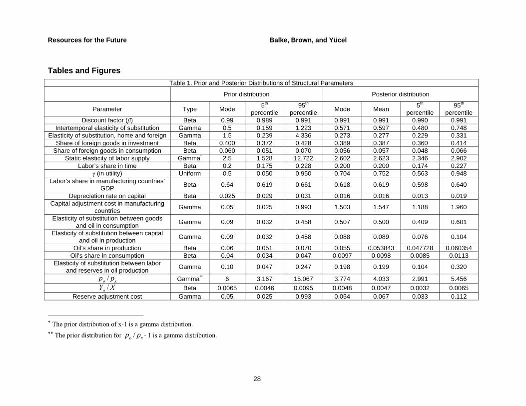
Table 1 displays the prior and estimated posterior distributions of the structural parameters. For many parameters, using the information in the data results in a substantial shift in the posterior distribution relative to the prior distribution; for most parameters the posterior distribution is substantially tighter than the prior distribution. Not surprisingly given the tight priors for these parameters, the posterior distributions for the discount factor, labor’s share in manufacturing-country GDP, the share of home and foreign goods, oil’s share in production, and the depreciation rate on capital are similar to the prior distributions of those parameters. One exception is the posterior distribution for the share of oil in consumption; it shifts toward lower values compared with the prior distribution (interior 90 percent of [.0085, .0113] for the posterior distribution versus [.034, .047] for the prior distribution).

Our posterior distribution suggests an estimate of the intertemporal elasticity of substitution that is similar to that typically assumed in the macroeconomics literature. Similarly, the posterior distribution of the elasticity of substitution between capital and oil is centered around a value similar to that assumed by Backus and Crucini. On the other hand, the posterior distribution also suggests an elasticity of substitution between domestic and foreign goods that is substantially lower than that typically assumed in open-economy DSGE models.7 Note that the

7 The dramatic swings in the relative import price over our sample period likely contribute to a relatively low value for the elasticity of substitution between home and foreign goods.


11

posterior distributions for most of these elasticities are substantially “tighter” than their prior distributions. Finally, the adjustment costs for capital are estimated to be substantially higher than those for oil reserves, suggesting that it is easier to add to reserves than it is to add to capital in the manufacturing country.

A key parameter in the utility function is γ. We employed a flat prior distribution centered around 0.5 for this parameter, but the posterior distribution is substantially tighter and centered around 0.75. This suggests that the utility function for our representative agent is closer to the standard King et al. (1988) preferences than to the Greenwood et al. (1988) preferences. This estimated value has implications for the response of U.S. (and ROW) GDP to an oil production shock.

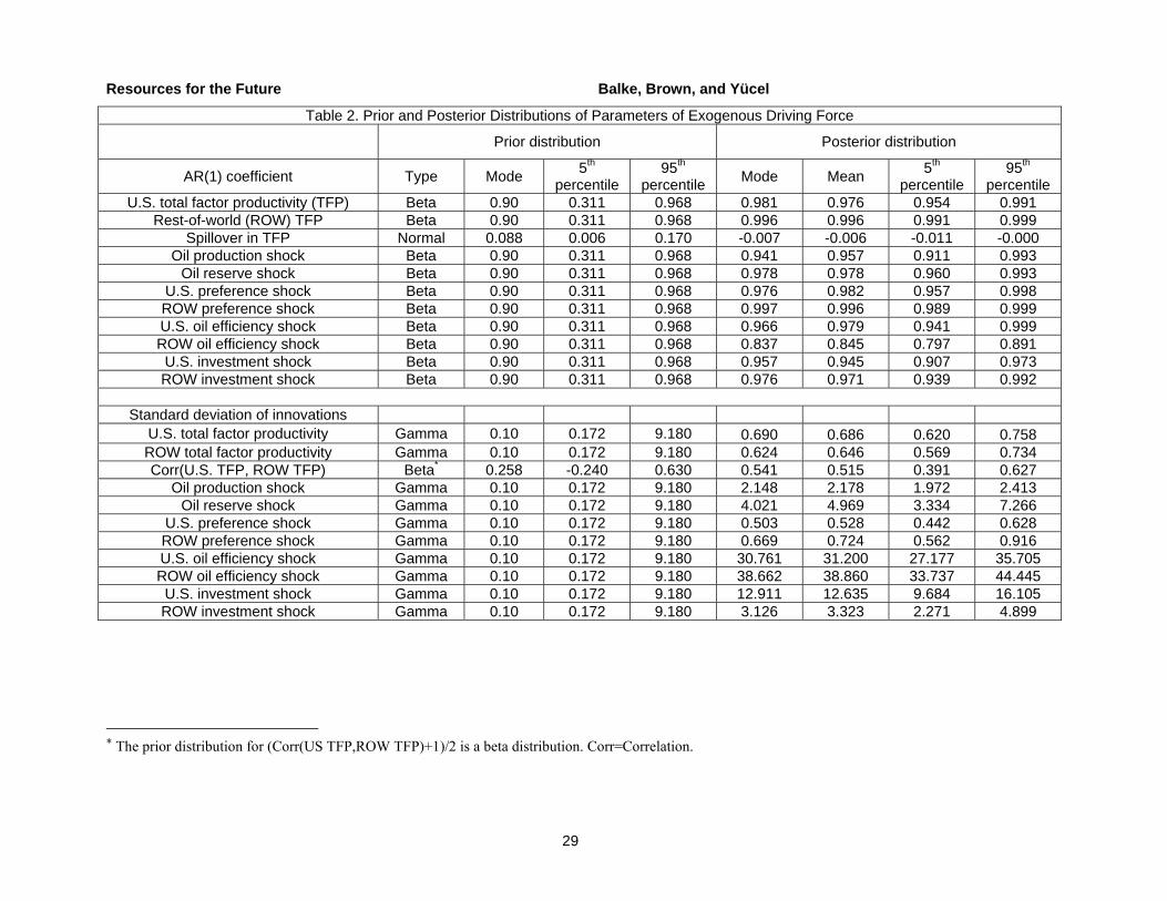
Table 2 presents the prior and posterior distributions for the stochastic processes governing the exogenous variables in the model. Given that prior distributions were relatively uninformative, the data have much to say about these parameters. The autoregressive parameters are quite high, suggesting that shocks are very persistent. The standard deviation of shocks to oil production and oil reserves is relatively large compared to shocks in total factor productivity and investment shocks in the manufacturing countries. The standard deviation of the oil efficiency shocks in the two manufacturing countries is very large, suggesting that these two variables may be an important source of shocks to world oil demand. On the other hand, the estimated spillover in total productivity is relatively small.

4. Estimated Impulse Responses

To obtain a better picture of what the model implies about the sources of oil price fluctuations, we examine how oil markets respond to a variety of shocks, including an oil production shock, an oil reserve shock, U.S. and ROW total factor productivity shocks, U.S. and ROW labor–leisure preference shocks, U.S. and ROW oil efficiency shocks, and U.S. and ROW investment shocks. We also examine in some detail how various aspects of U.S. activity respond to oil production and oil reserve shocks. For each series, we report the mean, fifth, and ninety-fifth percentile of the posterior distribution of the impulse responses.8

8 The impulse responses are the percentage change in each variable for a 1-percent change in the exogenous shock.


12

4.1 Responses of the Oil Market to Structural Shocks

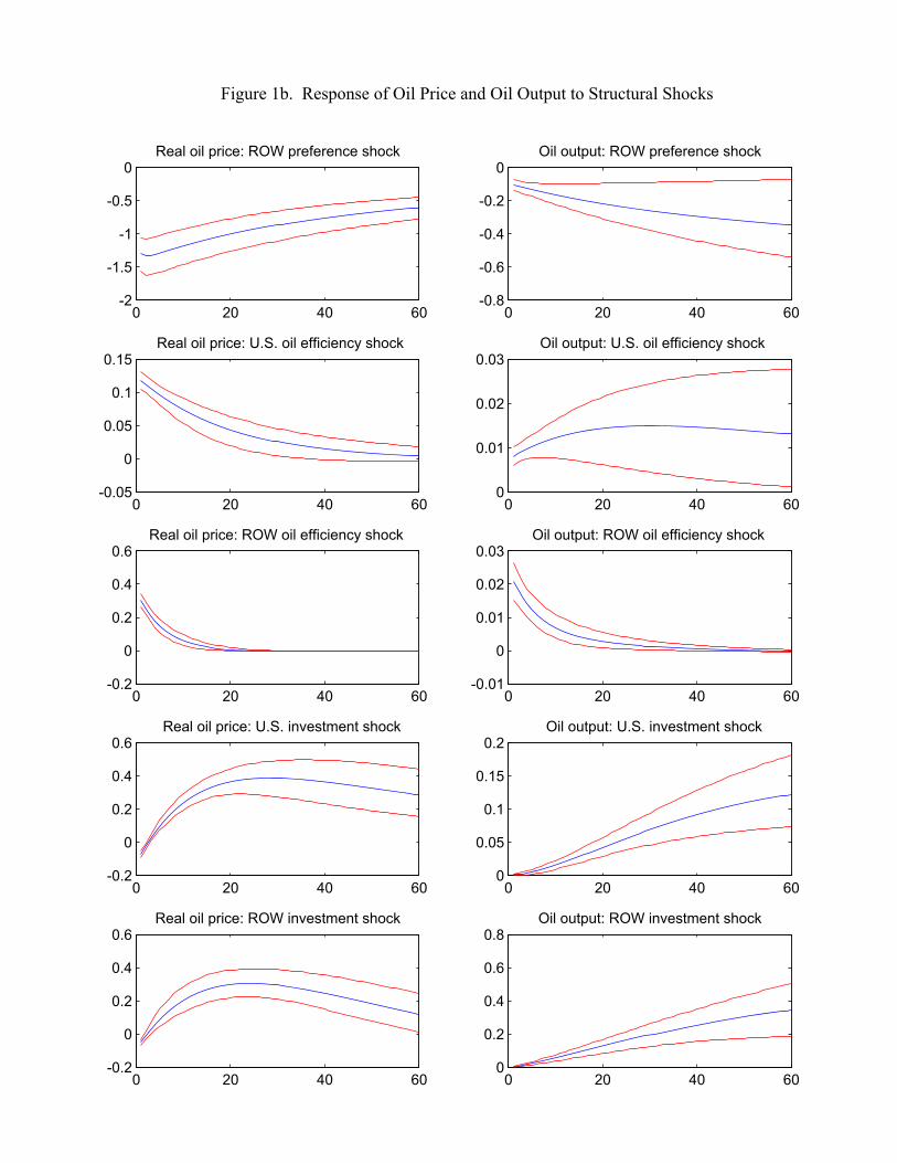
We find that oil production shocks yield oil-market dynamics that are like the classic supply shock envisioned in most economic research. As shown in Figure 1a, a positive oil production shock lowers the price of oil and boosts oil output. As the shock dissipates, oil price and oil output return toward their steady state values. Similarly, a favorable shock to the technology for adding reserves leads to higher oil output and lower oil prices, but these shocks take longer to have a substantial effect and have a longer-lived effect on oil prices and oil output.

The other eight shocks create what mostly can be described as shifts in oil demand (Figures 1a and 1b). A total factor productivity shock in the United States increases the real oil price and oil output, reminiscent of an increase in oil demand. An increase in U.S. total factor productivity also expands U.S. output and increases the use of oil in production. It also decreases the relative scarcity of U.S. goods, pushing down the U.S. GDP deflator which is in the denominator of the real oil price variable.

On the other hand, a total factor productivity shock in ROW leads to a downward movement in oil prices and, at least initially, a negative effect on oil output. In part, this effect stems from the fact that the U.S. GDP deflator is in the denominator of real oil prices, and a ROW total factor productivity shock increases the relative scarcity of U.S. goods, driving up their price. Given complete risk sharing across countries and that the ROW accounts for about 65 percent of world economic activity in the model, all consumers share in the sizable income gains as a result of an increase in ROW total factor productivity. Consumers choose to take some of their increased productivity in the form of leisure rather than goods, which leads to reduced consumer use of energy throughout the world. Over time, however, the effect on oil output becomes positive, though insignificantly so.

A shock to U.S. or ROW labor–leisure preferences reduces hours worked and output (reducing GDP in the country in which the shock occurs). A U.S. shock initially looks like a negative supply shock for oil; weaker economic activity reduces oil consumption and output, but the relative price of oil is pushed upward as U.S. firms substitute oil for labor. Over the longer-term, this substitution drives up the real price of oil and oil output, making the effects look like a shift in oil demand. The oil market response to a ROW shock to labor–leisure preferences is somewhat different. For a ROW shock, the international income effect dominates, and the shock reduces oil demand. Both the real oil price and oil output are reduced.

An oil efficiency shock increases the productivity of oil (both in production and the consumption). Shocks to both U.S. and ROW oil efficiency raise the real oil price and oil output,


13

again reminiscent of an oil demand shock. For a shock to ROW oil efficiency, these effects are larger but shorter in duration than the effects of U.S. oil efficiency shocks.

Similarly, both U.S. and ROW investment shocks yield higher real oil prices and oil output after the initial period. Such a shock increases the productivity of investment in creating capital goods, which gradually increases GDP in the country where such a shock occurs. The initial effect for a U.S. investment shock is a slight decline in oil prices—the result of a decline in oil demand as the economy redirects resources away from consumption and toward investment. For a ROW investment shock, however, the initial effect is no change in oil prices. Over the longer term, the gains in investment from either a U.S. or ROW investment shock drive up oil demand, and the relative oil price and oil output rise.

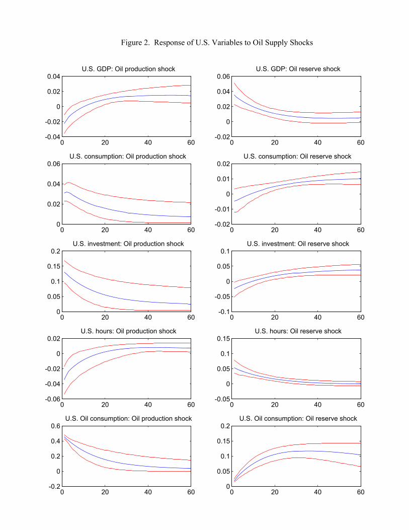
4.2 Oil Supply Shocks and U.S. Economic Activity

As modeled, there are two types of oil supply shocks: one that primarily affects current oil production and another that primarily affects future oil production. Figure 2 displays the responses of the U.S. variables used in estimating the model to these two oil supply shocks. Perhaps unexpectedly, a favorable oil production shock initially reduces U.S. GDP. Given the estimated value of 0.75 for the preference parameter, γ, and the use of oil in consumption, positive oil production shocks reduce the price of oil, which creates substantial positive income effects.9 These income effects yield an initial reduction of U.S. hours worked and U.S. GDP. As the effects of the oil production shock begin to dissipate, the income effect is reduced, and U.S. hours worked and GDP increase. As expected, both U.S. total consumption and U.S. oil consumption increase.

A favorable shock to the technology for building oil reserves (which also lowers oil prices and increases oil output) boosts U.S. GDP, U.S. hours worked, and U.S. oil consumption. U.S. total consumption and investment initially fall slightly as resources flow to investment in oil reserves.

Historically, one might consider oil supply shocks to be instances in which oil production and oil reserve shocks occurred at the same time. Taken together, the oil production and oil reserve shocks generate a negative relationship between oil prices and U.S. economic activity, as

9 When either γ or oil’s share in consumption are set close to zero, however, the income effect disappears, and U.S. hours worked and U.S. GDP strictly increase in response to a positive oil production shock.


14

the model estimates the standard deviation of oil reserve shocks to be roughly twice as large as that of oil production shocks. The combination of these two supply shocks implies an estimated posterior distribution for the oil price elasticity of U.S. real GDP with a mean of −0.016.10 The interior 90 percent of the posterior distribution for the elasticity is −0.011 to −0.022. These estimates are at the lower end of the range, −0.012 to −0.12, found by previous empirical research for the United States.11

Other shocks, such as those to U.S. preferences and oil efficiency, can also generate an inverse relationship between oil price fluctuations and U.S. output—although both yield a positive relationship between oil prices and oil output. Both a U.S. preference shock and oil efficiency shock reduce U.S. GDP while increasing the real oil price through increased oil demand. In contrast, shocks to U.S. total factor productivity, ROW preferences, ROW oil efficiency, and U.S. and ROW investment efficiency generate a positive relationship between oil price, oil output, and U.S. GDP. A shock to ROW total factor productivity generates a lower real world oil price and lower oil output while having an insignificant negative effect on U.S. GDP.

5. Historical Decompositions

Historical decompositions show the contribution of the various shocks to the evolution of oil prices, oil output, and U.S. real GDP. In each figure, we represent the history of the demeaned log of the oil price, the detrended log of oil output, or the detrended log of U.S. real GDP over the 40-year estimation period, as well as the mean, fifth percentile, and ninety-fifth percentile of the posterior distribution of the contribution of the exogenous shocks. The extent to which the posterior distribution moves with the historical series shows the extent to which the given variable explains the historical movement.

Impulse responses provide guidance to interpreting the historical decompositions. To identify historical episodes of unfavorable oil supply shocks that reduce U.S. GDP, we must identify periods during which the oil price rises and both oil output and U.S. GDP fall. On the other hand, the identification of oil demand shocks requires oil prices and oil output to move in the same direction. Depending on the nature of the shock creating a change in oil demand, U.S. GDP can rise or fall.

10 The estimated elasticity is the percentage change in U.S. GDP divided by the percentage change in the oil price. 11 See Jones et al. (2004).


15

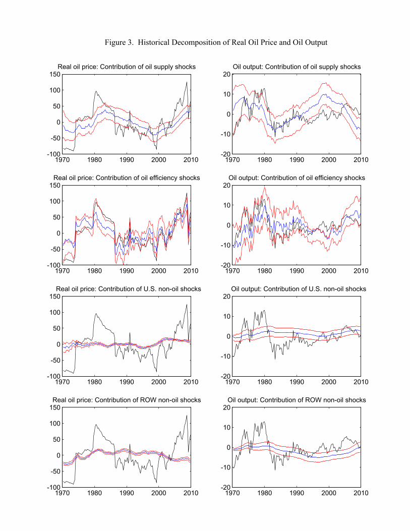
5.1 Real Oil Price and Oil Output

As shown in Figure 3, the historical decompositions suggest that both oil supply and oil demand shocks contributed to the historical movements of oil prices. Supply shocks (oil production and reserve shocks) are characterized by fairly long swings with supply falling in the late 1970s and early 1980s, rising from the early 1980s to about 2000, and falling thereafter. These oil supply changes contributed to the general rise of oil prices from the early 1970s to mid-1980s, the general decline in oil prices from the mid-1980s to about 2000, and the rise in prices that occurred from 2000 to 2008.

In contrast, demand shocks (in the form of oil efficiency shocks) contributed much of the volatility in oil prices and oil output seen from 1970 through 2009. Other U.S. and ROW shocks (total factor productivity, preference and investment shocks) play much lesser roles in the history of oil price and oil output movements, explaining only a general rise in oil prices from 1970 to the early 1980s.

Our finding that oil supply shocks do not explain much in the way of oil price movements is similar to conclusions reached by Barsky and Kilian (2002) and Kilian (2009). In examining the data, we find that over most of the sample period, oil prices and oil output do not move in a way that the model or theory would expect if oil supply shocks were important to oil price variation. Sharp declines in production do not accompany the sharp oil price increases from the 1970s into the early 1980s and then the 2000s. The path of least resistance, as far as the model is concerned, is to attribute the co-movements in oil prices and oil output to oil-specific demand shocks (oil efficiency shocks).

As modeled, an oil efficiency shock is a change in the productivity of oil in consumption and the production of capital services. According to the estimation, these oil efficiency shocks do not have a strong effect on either consumption or manufacturing output. Hence, oil efficiency shocks become an avenue for oil demand shocks that have very little spillover to other economic activity, which raises the possibility that oil efficiency shocks proxy other effects, such as speculative or precautionary oil demand.

5.2 U.S. Economic Activity

The historical decompositions show that oil supply shocks had very moderate effects on U.S. economic activity (Figure 4). Oil supply shocks contributed to a mild slowing of U.S. economic activity from the early 1970s to the early 1980s and a mild rise in activity from the mid-1980s to late 1990s, but they do not explain the volatility of U.S. economic activity. Given


16

that our model shows oil supply shocks have generated only mild, long-term swings in oil prices and oil output, it should not be surprising that the effect of such shocks on U.S. GDP was small.

The historical decompositions also show that ROW shocks are similarly moderate in their effects—even in those cases where ROW shocks have contributed to rising oil prices. Although the income gains and productivity spillovers to the United States are small, they offset any economic losses that arise from the effects of higher oil prices.

The historical decompositions identify U.S. shocks as being of the greatest importance to the evolution of U.S. GDP. With oil efficiency playing almost no role, U.S. preference, total factor productivity, and investment shocks show the greatest effects. Together these three effects explain much of the volatility in U.S. GDP in early 1970s. Total factor productivity drove a sharp decline in the early 1980s, and U.S. preference shocks drove U.S. GDP from the early 1980s through 2009, with investment efficiency also making important contributions to the swings.

5.3 Oil Prices and U.S. Economic Activity in the 1970s to Early 1980s and the 2000s

We find the relatively poor U.S. economic performance in the mid-1970s through the early 1980s largely resulted from shocks to total factor productivity, aided by preference and investment efficiency shocks. Oil supply shocks contributed only moderately to the poor economic performance, while ROW shocks contributed to the downdraft in the mid-1970s. These findings differ sharply from earlier studies, such as those by Hamilton (1983) and Balke et al. (2002), who found that oil price shocks had a substantial effect on economic activity without distinguishing between sources of oil price shocks or identifying the effect of other shocks on U.S. economic activity. In failing to consider these other factors, these earlier studies likely attributed too much of the economic loss to oil price shocks.

Our findings for the 1970s and early 1980s are somewhat stronger than but consistent with those of Greenwood and Yorukoglu (1997), Samaniego (2006), Blanchard and Gali (2007), and Kilian (2009). Kilian finds that oil supply shocks are of lesser importance to U.S. GDP than other sources of economic fluctuation. In contrast, Blanchard and Gali find the poor U.S. economic performance of the 1970s owes to a combination of adverse oil price shocks and other negative factors. Greenwood and Yorukoglu and Samaniego attribute some of the negative


17

productivity shocks of that era to significant learning costs associated with the adoption of new technologies and the necessity of plant-level reorganization.12

For the 1990s and 2000s, we find the strong growth in U.S. real GDP (and the subsequent recession) reflects several different domestic sources. The principal contribution was an investment boom that began in the mid-1990s. Gains in total factor productivity followed from about 2000 but were dulled as U.S. preferences shifted toward leisure. In the late 2000s, investment and preference shocks were the main contributors to the decline in U.S. GDP.13

These shocks originating in the United States only had moderate effects on oil prices. Oil supply shocks contributed to a general upward rise in oil prices without much effect on U.S. GDP. Oil efficiency shocks, both in the United States and ROW, are the major forces behind oil price fluctuations. These findings are similar to those of Kilian (2009) and Kilian and Hicks (2010), who find that growing world output has pushed oil prices upward. They are somewhat different from those by Blanchard and Gali (2007), who find that rising oil prices had small negative effects on output, which were generally dwarfed by other positive shocks in the 2000s.

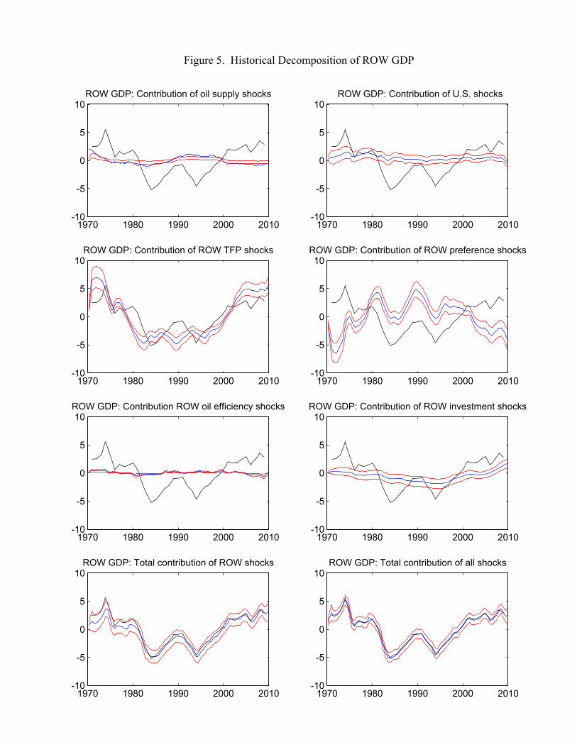
5.4 Sources of ROW Fluctuations

Although our focus has been primarily on oil price movements and U.S. economic activity, our model does have something to say about fluctuations in the rest of the world. Even though the model is quarterly and the ROW data are annual, the model tracks movements in ROW GDP (Figure 5). Oil supply and U.S. shocks explain relatively little of the fluctuations in ROW GDP. Fluctuations in ROW output fluctuations are driven primarily by ROW shocks, with total factor productivity and preferences being the most important. The dramatic gain in ROW GDP at the end of the sample can be mostly attributed to increases in ROW total factor productivity.

6. Model Robustness

We undertook a number of changes to the model specification to examine the robustness of our conclusions. These include re-estimating the model so that the income effects and

12 Some negative productivity shocks of the 1970s also may have resulted from the new and relatively inefficient environmental regulation introduced during that era. 13 The lack of a financial sector in the model forces it to attribute the decline in U.S. GDP in 2008–2009 to investment and preference shocks.


18

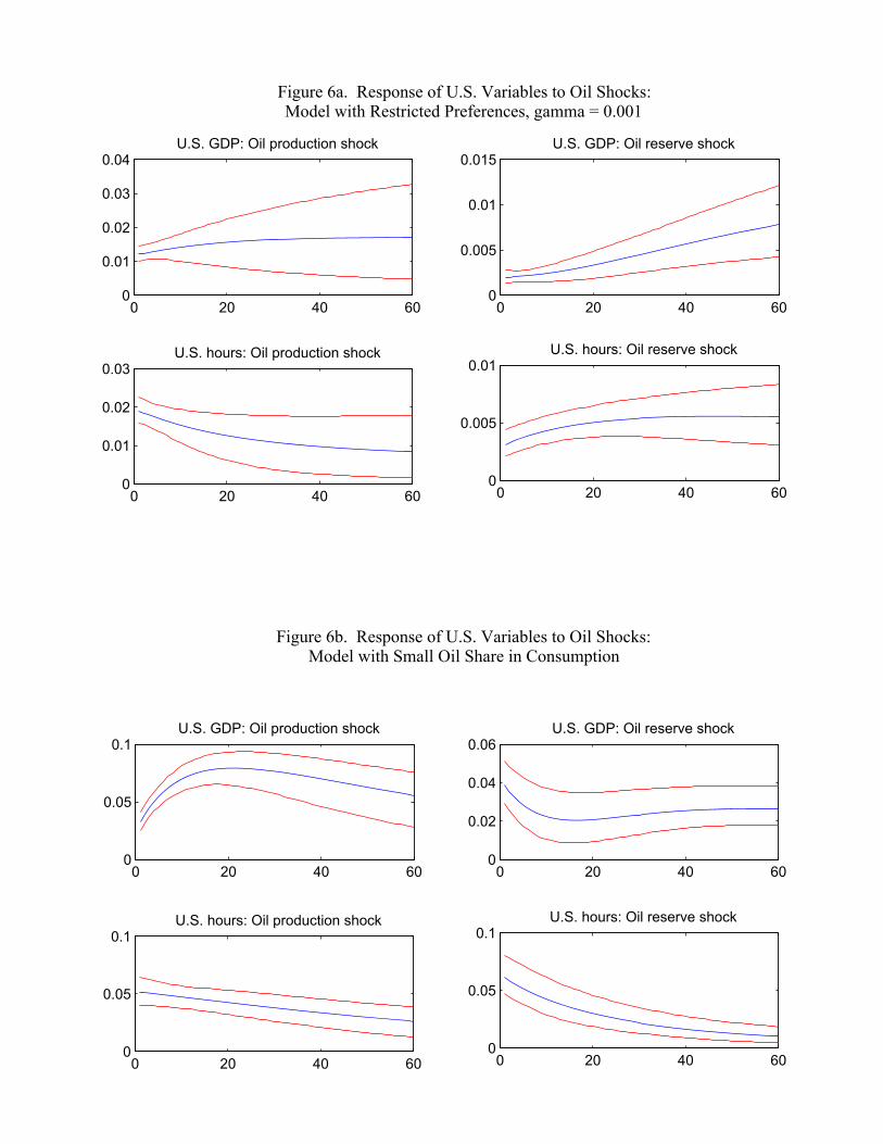
productivity shocks are constrained to be small, re-estimating the model so that the share of oil in consumption is small, replacing investment shocks with “news” shocks for total factor productivity in all three countries, and setting the variance of the oil efficiency shocks to be small. In all four cases, the resulting historical decompositions show very little change in the relationship between oil supply shocks and U.S. GDP. In some cases, the impulse responses and other historical decompositions are changed.

In keeping with Jaimovich and Rebelo (2009), we restrict γ to equal 0.001 so that the income effect is small, and re-estimate the model. With this restriction, the response of U.S. hours worked and GDP to a positive oil production shock are somewhat different from our base case. With the income effect limited, a positive oil production shock increases hours worked and U.S. GDP increases. Consequently, oil supply shocks have a larger effect on U.S. GDP (Figure 6a). Nonetheless, the historical decompositions are largely unaffected by restricting γ to be small.

Similarly, we set oil’s share in consumption to be 0.001 and re-estimate the model. Again, the response of U.S. hours and GDP to a positive oil production shock is positive (Figure 6b). Dropping oil out of consumption lessens the income effect of an oil supply shock, and the substitution effects dominate. Once again, the historical decompositions are largely unaffected.

We also replaced investment shocks with a “news” shock about future total factor productivity shocks for all three countries. The estimated parameters and historical decompositions are largely unchanged. The estimated posterior distribution for γ suggests a substantial income effect, and, as a result, favorable news about future oil production results in a decrease in current hours and production (both in manufacturing and oil-producing countries). Again, historical decompositions suggest oil efficiency shocks are largely responsible for oil price fluctuations and that neither oil supply shocks nor oil efficiency shocks have much effect on U.S. GDP.

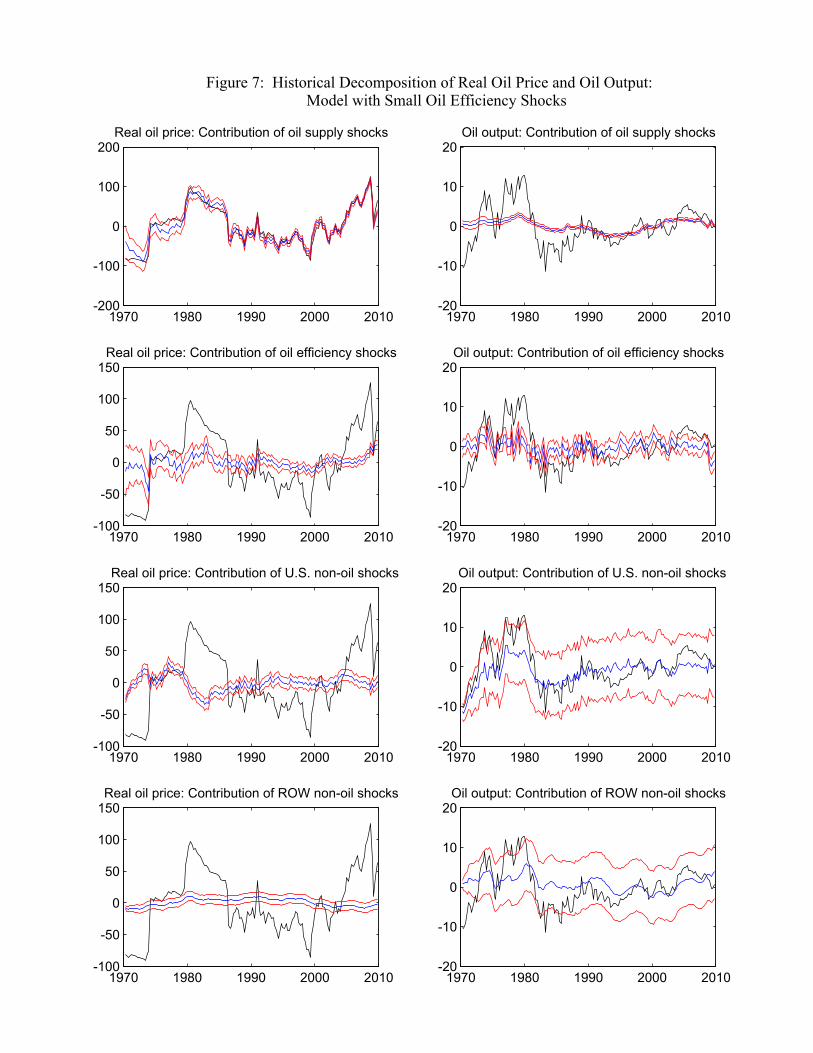
Because our benchmark model finds oil efficiency shocks to be responsible for most of the fluctuations in oil prices and oil output, we examined the role of such shocks by setting their variance to be small.14 When oil efficiency shocks have small variances, the historical decompositions show that supply shocks drive most of the fluctuations in oil prices, but oil output is still largely driven by demand shocks—including those to oil efficiency, total factor

14 Formally, we assume a tight prior distribution for these standard deviations. We set the model of the prior distributions to be 0.001.


19

productivity, preferences, and investment (Figure 7). These findings are consistent with the idea that episodic rises in oil prices bear relatively little relationship with falling oil output. In this specification, the elasticities of substitution between oil and goods and oil and capital are estimated to be very small; oil demand is extremely inelastic. As a result, the model attributes oil price movements to oil supply shocks and oil output movements to oil demand shocks. As with the other cases, the effect of oil supply shocks on U.S. GDP is unimpressive.

7. Conclusions

Economic history has provided seemingly contradictory evidence about the relationship between oil price movements and aggregate U.S. economic activity. Oil prices rose sharply in the 1970s and early 1980s, and U.S. economic activity contracted sharply. Oil prices rose strongly throughout much of the 2000s, but U.S. economic activity continued to expand until recession hit in early 2008.

Previous research has offered a number of different reasons for these contradictory historical experiences. One explanation is that the 2000s were characterized by productivity-driven oil demand shocks that yielded a positive relationship between oil prices and economic activity, while the 1970s and early 1980s were characterized by oil supply shocks that yielded an inverse relationship between oil prices and economic activity. Another is that substantially different factors shape the movements in oil prices and U.S. GDP, and those factors combine differently over time, creating the appearances of an inverse relationship in the earlier period and a positive relationship in the latter period.

We find evidence supporting both explanations, but with much greater weight on the latter. Oil supply and oil efficiency shocks have been the primary drivers oil prices, but such shocks have had relatively little effect on U.S. GDP. Total factor productivity, preference, and investment efficiency shocks have been the primary drivers of fluctuations in U.S. GDP, but these shocks have had relatively small effects on oil prices. Nonetheless, we find that oil supply shocks contributed a drag to U.S. economic activity in the 1970s and early 1980s. We also find that oil demand shocks played a somewhat bigger role in the oil price increases of the 2000s than those of the 1970s and early 1980s.

U.S. GDP fell sharply after the oil price increases in the 1970s and early 1980s, primarily because shocks to U.S. productivity reduced output. Oil supply shocks mildly reinforced that economic weakness. By not taking into account the possibility of domestic shocks, some of the earlier literature likely overestimates the effects that oil supply shocks had on economic activity.


20

U.S. GDP continued to rise as oil prices rose in the 2000s because changes in U.S. investment efficiency, total factor productivity, and preferences completely overwhelmed the extremely mild drag contributed by oil supply shocks.


21

References

Backus, David K., and Mario J. Crucini. 2000. Oil Prices and the Terms of Trade. Journal of International Economics 50: 185–213.

Balke, Nathan S., Stephen P. Brown, and Mine K. Yücel. 2002. Oil Price Shocks and the U.S. Economy: Where Does the Asymmetry Originate? The Energy Journal 23(3): 27–52.

Barsky, Robert, and Lutz Killian. 2002. Do We Really Know that Oil Caused the Great Stagflation? A Monetary Alternative. NBER Macroeconomics Annual 2001: 137–83.

Barsky, Robert, and Lutz Killian. 2004. Oil and the Macroeconomy since the 1970s. Journal of Economic Perspectives 18(4): 115–34.

Blanchard, Olivier, and J. Gali. 2007. The Macroeconomic Effects of Oil Price Shocks: Why Are the 2000s So Different from the 1970s? Working paper 07-21. Cambridge, MA: Massachusetts Institute of Technology, Department of Economics.

Blanchard, O., and C. Kahn. 1980. The Solution of Linear Difference Equations under Rational Expectations. Econometrica 48: 1305–10.

Bodenstein, Martin, Christopher J. Erceg, and Luca Guerrieri. 2007. Oil Shocks and External Adjustment. International finance discussion paper 897. Washington, DC: Board of Governors of the Federal Reserve System.

Brown, Stephen P.A., and Mine K. Yücel. 2002. Energy Prices and Aggregate Economic Activity: An Interpretative Survey. Quarterly Review of Economics and Finance 42(2): 193–08.

Congressional Budget Office. 2006. The Economic Effects of Recent Increases in Energy Prices. Publication #2835. Washington, DC: Congressional Budget Office.

Edelstein, Paul, and Lutz Kilian. 2007. The Response of Business Fixed Investment to Changes in Energy Prices: A Test of Some Hypotheses About the Transmission of Energy Price Shocks. The B.E. Journal of Macroeconomics 7(1): Article 35.

Greenwood, Jeremy, Zvi Hercowitz, and Gregory Huffman. 1988. Investment, Capacity Utilization, and the Real Business Cycle. American Economic Review 78(3): 402–17.

Greenwood, Jeremy, and Mehmet Yorukoglu. 1997. 1974. Carnegie-Rochester Conference Series on Public Policy 46: 49–95.


22

Herrera, Ana Maria, and Elena Pesavento. 2009. Oil Price Shocks, Systematic Monetary Policy and the “Great Moderation.” Macroeconomic Dynamics 13(1): 109–37.

Hamilton, James D. 1983. Oil and the Macroeconomy since World War II. Journal of Political Economy 91(2): 228–48.

Hickman, Bert, Hillard Huntington, and James Sweeney, eds. 1987. Macroeconomic Impacts of Energy Shocks. Amsterdam, The Netherlands: North-Holland.

Huntington, Hillard. 2003. Energy Disruptions, Interfirm Price Effects and the Aggregate Economy. Energy Economics 25(2), 119–36.

Jaimovich, Nir, and Sergio Rebelo. 2009. Can News About the Future Drive the Business Cycle? American Economic Review 99(4): 1097–118.

Jones, Donald W., Paul N. Leiby, and Inja K. Paik. 2004. Oil Price Shocks and the Macroeconomy: What Has Been Learned Since 1996? The Energy Journal 25(2): 1–32.

Kilian, Lutz. 2008a. A Comparison of Effects of Exogenous Oil Supply Shocks on Output and Inflation in the G7 Countries. Journal of the European Economic Association 61(1): 78–121.

Kilian, Lutz. 2008b. Exogenous Oil Supply Shocks: How Big Are They and How Much Do They Matter for the U.S. Economy? Review of Economics and Statistics 90(2): 216–40.

Kilian, Lutz. 2008c. The Economic Effects of Energy Price Shocks. Journal of Economic Literature 46(4): 871–909.

Kilian, Lutz. 2009. Not All Oil Price Shocks Are Alike: Disentangling Demand and Supply Shocks in the Crude Oil Market. American Economic Review 99(4): 1053–69.

Kilian, Lutz, and Bruce Hicks. 2010. Did Unexpectedly Strong Economic Growth Cause the Oil Price Shock of 2003–2008? Mimeo. Ann Arbor, MI: University of Michigan.

King, Robert G., Charles I. Plosser, and Sergio Rebelo. 1988. Production, Growth and the Business Cycles: I. The Basic Neoclassical Model. Journal of Monetary Economics 21 (2/3): 195–232.

Lubik, T., and F. Schorfheide. 2004. Testing for Indeterminacy: An Application to U.S. Monetary Policy. American Economic Review 94(1): 190–217.

Mork, Knut Anton, and Robert E. Hall. 1980. Energy Prices, Inflation, and Recession, 1974–1975. The Energy Journal 1(3): 31–63.


23

Nakov, Anton, and Andrea Pescatori. 2007a. Oil and the Great Moderation. Working paper 0735. Madrid, Spain: Banco de España.

Nakov, Anton, and Andrea Pescatori. 2007b. Inflation-Output Gap Trade-Off with a Dominant Oil Supplier. Working paper 0723. Madrid, Spain: Banco de España.

Rasche, R.H., and J.A. Tatom. 1977. The Effects of the New Energy Regime on Economic Capacity, Production and Prices. Economic Review 59(4): 2–12.

Samaniego, Roberto M. 2006. Organizational Capital, Technology Adoption and the Productivity Slowdown. Journal of Monetary Economics 53(7): 1555–69.

Segal, Paul. 2007. Why Do Oil Price Shocks No Longer Shock? Oxford Institute for Energy Studies Working Paper WPM 35. Oxford, U.K.: University of Oxford.

Smets, F., and R. Wouters. 2007. Shocks and Frictions in U.S. Business Cycles: A Bayesian DSGE Approach. American Economic Review 97(3): 586–606.

Stock, James H., and Mark W. Watson. 2003. Has the Business Cycle Changed? Evidence and Explanations. Paper presented at the Federal Reserve Bank of Kansas City Symposium. August 28–30, Jackson Hole, Wyoming.


24

Technical Appendix

A. Observation Equations in the State-Space Model

Our data consists of observations on U.S. GDP, consumption, investment, and employment, the relative (non-oil) import price for the United States, U.S. oil consumption (barrels), real oil price (deflated by U.S. GDP deflator), world oil production (barrels), rest-of-world (ROW) real GDP in U.S. dollars as measured by purchasing power parity (PPP), and ROW real investment in U.S. dollars as measured by PPP. For several variables, the mapping between the model and the data are exact: ˆ Y us,t

cons = ˆ C a,t , ˆ Y us,tinv = ˆ I a ,t , ˆ Y ROW ,t

inv = ˆ I b ,t , ˆ Y us,t

emp = ˆ N a,t , ˆ Y oil output ,t = ˆ Y o,t , and ˆ Y us,t

oil cons = ˆ O a,t . However, several variables need to be transformed to

correspond to the data we will employ. Output in the model corresponds to gross output rather

than value added, thus GDP is given by ˆ Y row,tgdp = ( ˆ Y b,t −

PoOb

PbYa

ˆ O b,t ) /(1−PoOb

PbYb

) and

ˆ Y us,tgdp = ( ˆ Y a,t −

PoOa

PaYa

ˆ O a,t ) /(1−PoOa

PaYa

). Similarly, as the GDP (value added) deflator was used to

deflate the import price and oil price, ˆ Y us,trel import price = ( ˆ P b ,t − ˆ P a,t ) + ( ˆ P o,t − ˆ P a,t )

PoOa

PaYa

1− PoOa

PaYa

, and

ˆ Y real oil price,t = ( ˆ P o,t − ˆ P a,t ) /(1−PoOa

PaYa

).

B. Bayesian Estimation of the DSGE Model

One can write the solution to the linearized, rational expectations dynamic stochastic general equilibrium (DSGE) model in terms of a state-space model: Yt

mod el = ΠStmod el , (B1)

St = MSt−1 + Vtmod el , (B2)

where Ytmod el

is a vector of endogenous variables in the model; S tmod el is the state vector that

includes the capital stocks of the United States (country a) and ROW (country b), oil reserves, and the ten exogenous shock variables: oil production shocks; oil reserve shocks; and total factor productivity, labor–leisure preferences, oil efficiency, and investment (capital accumulation) shocks for countries a and b.

The model is written in terms of quarters, but we have only annual data for ROW GDP and ROW investment. Thus, we partition the observation equation of the state-space model into


25

two sets of equations—one corresponding to quarterly observations, the other corresponding to annual observations. The observation equation is given by:

Ytobs =

Ytquarterly

Ytannual

⎛

⎝ ⎜

⎞

⎠ ⎟ =

Π1 0 0 0.25Π2 .25Π2 .25Π2 .25Π2

⎛

⎝ ⎜

⎞

⎠ ⎟

Stmod el

St−1mod el

St−2mod el

St−3mod el

⎛

⎝

⎜ ⎜ ⎜ ⎜

⎞

⎠

⎟ ⎟ ⎟ ⎟

. (B3)

The corresponding state equation is given by:

Stmod el

St−1mod el

St−2mod el

St−3mod el

⎛

⎝

⎜ ⎜ ⎜ ⎜

⎞

⎠

⎟ ⎟ ⎟ ⎟

=

M 0 0 0I 0 0 00 I 0 00 0 I 0

⎛

⎝

⎜ ⎜ ⎜ ⎜

⎞

⎠

⎟ ⎟ ⎟ ⎟

St−1mod el

St−2mod el

St−3mod el

St−4mod el

⎛

⎝

⎜ ⎜ ⎜ ⎜

⎞

⎠

⎟ ⎟ ⎟ ⎟

+

Vtmod el

000

⎛

⎝

⎜ ⎜ ⎜ ⎜

⎞

⎠

⎟ ⎟ ⎟ ⎟

. (B4)

The empirical state space model implied by (B3) and (B4) can be rewritten as: Yt

obs = H(θ)St +Wt , Wt ~ MVN (0,R) , (B5)

St = F (θ)St−1 + Vt ,Vt ~ MVN (0,Q(θ)) , (B6)

where obstY is the vector of observable time series, tS is the vector of unobserved state variables,

and θ is the vector of structural parameters in the DSGE model. In our application, obstY contains

detrended quarterly per capita real U.S. GDP, detrended quarterly per capita real U.S. consumption, detrended quarterly per capita real U.S. investment, detrended per capita quarterly U.S. oil consumption, detrended quarterly world oil production, demeaned quarterly real oil price, detrended quarterly real non-oil import price for the United States, detrended annual real GDP for ROW (PPP constant U.S. dollars), and detrended annual real investment expenditures for ROW (PPP constant U.S. dollars). We scale up all the variables by 100. We set R to be a diagonal matrix with diagonal elements equal to10 −4 . We treat observations for the annual data as missing for all but the fourth quarter of the year.

Given the parameters,θ , we can estimate the unobserved states by the Kalman Filter. The predictive log likelihood of the state space model is given by:

l(YT ,θ) = {−.5log(det(H(θ)'Pt |t−1H(θ) + R))t=1

T

∑

− .5(Yt − H(θ)St |t−1)'(H(θ)'Pt |t−1H(θ) + R)−1(Yt − H(θ)St |t−1)}, (B7)


26

where St | t−1 and 1−t|tP are the conditional mean and variance of tS from the Kalman filter.

Given a prior distribution over parameters, h(θ ) , the posterior distribution, P(θ | YT ) , is P(θ | YT ) ∝ exp( l(YT ,θ))h(θ) . (B8)

Because the log-likelihood is a highly nonlinear function of the structural parameter vector, it is not possible to write an analytical expression for the posterior distribution. As a result, we use Bayesian Markov Chain Monte Carlo methods to estimate the posterior distribution of the parameter vector, θ . In particular, we employ a Metropolis-Hasting sampler to generate draws from the posterior distributions. The algorithm is as follows:

(i) Given a previous draw of the parameter vector, θ ( i−1) , draw a candidate vector cθ

from the distribution g(θ |θ ( i−1)) .

(ii) Determine the acceptance probability for the candidate draw,

α(θ c,θ ( i−1)) = min exp( l(YT ,θ(c )))h(θ(c ))exp( l(YT ,θ (i−1)))h(θ( i−1))

g(θ (i−1) |θ c )g(θ c |θ(i−1))

, 1⎡

⎣ ⎢

⎤

⎦ ⎥ .

(iii) Determine a new draw from the posterior distribution, θ ( i).

θ ( i) = θ c with probability α(θ c,θ ( i−1)) ,

θ ( i ) = θ ( i−1) with probability 1− α(θ c,θ ( i−1)) .

(iv) Return to (i).

Starting from an initial parameter vector and repeating enough times, the distribution parameters draws, θ ( i), will converge to the true posterior distribution.

In our application, θ c = θ ( i−1) + v , where v is drawn from a multivariate t-distribution with 50 degrees of freedom and a covariance matrix Σ . We set Σ to be a scaled value of the Hessian matrix of − l(YT ,θ)) − ln(h(θ)) evaluated at the posterior mode. We choose the scaling so that around 50 percent of the candidate draws are accepted. We run five separate Markov Chains, each with a different initial condition. For each chain, we set a burn-up period of 100,000 draws and then sample every tenth draw for a total of 10,000 draws. Thus, the posterior distribution of parameters is based on a total of 100,000 draws. We also obtain the posterior distributions for the unobserved states. Given a parameter draw, we draw from the conditional posterior distribution


27

for the unobserved states, P(ST | Θ( i),YT ) . Here we use the “filter forward, sample backwards” approach proposed by Carter and Kohn (1994) and discussed in Kim and Nelson (1999).

C. Data Sources for ROW

To obtain an approximate estimate of the data for the rest-of-world oil-consuming country, ROW, we aggregate data from 29 countries—Brazil, China, and India, plus 26 of the 30 Organisation for Economic Co-operation and Development (OECD) countries. We exclude the United States, whose data is used for the home country in the model; Mexico, which is a major oil-producing country; and the Czech Republic and Slovakia, neither of which have reliable data prior to 1990. Because real GDP and investment are reported in U.S. dollars, we aggregate these series across countries. We convert ROW GDP and investment to per capita series by dividing with population aggregated across countries.

For the period 1970 to 2003, the data for population, real GDP, and real investment for all 29 countries are taken from the Penn World Table. For the period 2004 through 2008, the data for the 26 OECD countries are from the OECD; and the data for Brazil, India, and China are from Haver Analytics. The data from 2004 to 2008 were spliced to the earlier data in 2003, country by country, and then aggregated to obtain per capita measures of ROW output and investment.

References

Carter, C.K., and R. Kohn. 1994. On Gibbs Sampling for State Space Models. Biometrika 81(3): 541–53.

Kim, Chang-Jin, and Charles Nelson. 1999. Has the U.S. Economy Become More Stable? A Bayesian Approach Based on a Markov-Switching Model of the Business Cycle. Review of Economics and Statistics 81(4): 608–16.


28

Tables and Figures Table 1. Prior and Posterior Distributions of Structural Parameters

Prior distribution Posterior distribution

Parameter Type Mode 5th percentile

95th percentile Mode Mean 5th

percentile 95th

percentile Discount factor (β) Beta 0.99 0.989 0.991 0.991 0.991 0.990 0.991

Intertemporal elasticity of substitution Gamma 0.5 0.159 1.223 0.571 0.597 0.480 0.748 Elasticity of substitution, home and foreign Gamma 1.5 0.239 4.336 0.273 0.277 0.229 0.331

Share of foreign goods in investment Beta 0.400 0.372 0.428 0.389 0.387 0.360 0.414 Share of foreign goods in consumption Beta 0.060 0.051 0.070 0.056 0.057 0.048 0.066

Static elasticity of labor supply Gamma* 2.5 1.528 12.722 2.602 2.623 2.346 2.902 Labor’s share in time Beta 0.2 0.175 0.228 0.200 0.200 0.174 0.227

γ (in utility) Uniform 0.5 0.050 0.950 0.704 0.752 0.563 0.948 Labor’s share in manufacturing countries’

GDP Beta 0.64 0.619 0.661 0.618 0.619 0.598 0.640

Depreciation rate on capital Beta 0.025 0.029 0.031 0.016 0.016 0.013 0.019 Capital adjustment cost in manufacturing

countries Gamma 0.05 0.025 0.993 1.503 1.547 1.188 1.960

Elasticity of substitution between goods and oil in consumption Gamma 0.09 0.032 0.458 0.507 0.500 0.409 0.601

Elasticity of substitution between capital and oil in production Gamma 0.09 0.032 0.458 0.088 0.089 0.076 0.104

Oil’s share in production Beta 0.06 0.051 0.070 0.055 0.053843 0.047728 0.060354 Oil’s share in consumption Beta 0.04 0.034 0.047 0.0097 0.0098 0.0085 0.0113

Elasticity of substitution between labor and reserves in oil production Gamma 0.10 0.047 0.247 0.198 0.199 0.104 0.320

po / px Gamma** 6 3.167 15.067 3.774 4.033 2.991 5.456 Yo / X Beta 0.0065 0.0046 0.0095 0.0048 0.0047 0.0032 0.0065

Reserve adjustment cost Gamma 0.05 0.025 0.993 0.054 0.067 0.033 0.112

* The prior distribution of x-1 is a gamma distribution. ** The prior distribution for po / px - 1 is a gamma distribution.


29

Table 2. Prior and Posterior Distributions of Parameters of Exogenous Driving Force Prior distribution Posterior distribution

AR(1) coefficient Type Mode 5th percentile

95th percentile Mode Mean 5th

percentile 95th

percentile U.S. total factor productivity (TFP) Beta 0.90 0.311 0.968 0.981 0.976 0.954 0.991

Rest-of-world (ROW) TFP Beta 0.90 0.311 0.968 0.996 0.996 0.991 0.999 Spillover in TFP Normal 0.088 0.006 0.170 -0.007 -0.006 -0.011 -0.000

Oil production shock Beta 0.90 0.311 0.968 0.941 0.957 0.911 0.993 Oil reserve shock Beta 0.90 0.311 0.968 0.978 0.978 0.960 0.993

U.S. preference shock Beta 0.90 0.311 0.968 0.976 0.982 0.957 0.998 ROW preference shock Beta 0.90 0.311 0.968 0.997 0.996 0.989 0.999 U.S. oil efficiency shock Beta 0.90 0.311 0.968 0.966 0.979 0.941 0.999 ROW oil efficiency shock Beta 0.90 0.311 0.968 0.837 0.845 0.797 0.891 U.S. investment shock Beta 0.90 0.311 0.968 0.957 0.945 0.907 0.973 ROW investment shock Beta 0.90 0.311 0.968 0.976 0.971 0.939 0.992

Standard deviation of innovations

U.S. total factor productivity Gamma 0.10 0.172 9.180 0.690 0.686 0.620 0.758 ROW total factor productivity Gamma 0.10 0.172 9.180 0.624 0.646 0.569 0.734 Corr(U.S. TFP, ROW TFP) Beta* 0.258 -0.240 0.630 0.541 0.515 0.391 0.627

Oil production shock Gamma 0.10 0.172 9.180 2.148 2.178 1.972 2.413 Oil reserve shock Gamma 0.10 0.172 9.180 4.021 4.969 3.334 7.266

U.S. preference shock Gamma 0.10 0.172 9.180 0.503 0.528 0.442 0.628 ROW preference shock Gamma 0.10 0.172 9.180 0.669 0.724 0.562 0.916 U.S. oil efficiency shock Gamma 0.10 0.172 9.180 30.761 31.200 27.177 35.705 ROW oil efficiency shock Gamma 0.10 0.172 9.180 38.662 38.860 33.737 44.445 U.S. investment shock Gamma 0.10 0.172 9.180 12.911 12.635 9.684 16.105 ROW investment shock Gamma 0.10 0.172 9.180 3.126 3.323 2.271 4.899

* The prior distribution for (Corr(US TFP,ROW TFP)+1)/2 is a beta distribution. Corr=Correlation.

0 20 40 60-4

-2

0

2Real oil price: Oil production shock

0 20 40 60-0.5

0

0.5

1Oil output: Oil production shock

0 20 40 60-1

-0.5

0Real oil price: Oil reserve shock

0 20 40 600

0.1

0.2

0.3

0.4Oil output: Oil reserve shock

0 20 40 60-1

0

1

2

3Real oil price: U.S. TFP shock

0 20 40 600

0.2

0.4

0.6

0.8Oil output: U.S. TFP shock

0 20 40 60-2.5

-2

-1.5

-1Real oil price: ROW TFP shock

0 20 40 60-0.1

0

0.1

0.2

0.3Oil output: ROW TFP shock

0 20 40 60-0.5

0

0.5

1Real oil price: U.S. preference shock

0 20 40 60-0.05

0

0.05

0.1

0.15Oil output: U.S. preference shock

Figure 1a. Response of Oil Price and Oil Output to Structural Shocks

0 20 40 60-2

-1.5

-1

-0.5

0Real oil price: ROW preference shock

0 20 40 60-0.8

-0.6

-0.4

-0.2

0Oil output: ROW preference shock

0 20 40 60-0.05

0

0.05

0.1

0.15Real oil price: U.S. oil efficiency shock

0 20 40 600

0.01

0.02

0.03Oil output: U.S. oil efficiency shock

0 20 40 60-0.2

0

0.2

0.4

0.6Real oil price: ROW oil efficiency shock

0 20 40 60-0.01

0

0.01

0.02

0.03Oil output: ROW oil efficiency shock

0 20 40 60-0.2

0

0.2

0.4

0.6Real oil price: U.S. investment shock

0 20 40 600

0.05

0.1

0.15

0.2Oil output: U.S. investment shock

0 20 40 60-0.2

0

0.2

0.4

0.6Real oil price: ROW investment shock

0 20 40 600

0.2

0.4

0.6

0.8Oil output: ROW investment shock

Figure 1b. Response of Oil Price and Oil Output to Structural Shocks

0 20 40 60-0.04

-0.02

0

0.02

0.04U.S. GDP: Oil production shock

0 20 40 60-0.02

0

0.02

0.04

0.06U.S. GDP: Oil reserve shock

0 20 40 600

0.02

0.04

0.06U.S. consumption: Oil production shock

0 20 40 60-0.02

-0.01

0

0.01

0.02U.S. consumption: Oil reserve shock

0 20 40 600

0.05

0.1

0.15

0.2U.S. investment: Oil production shock

0 20 40 60-0.1

-0.05

0

0.05

0.1U.S. investment: Oil reserve shock

0 20 40 60-0.06

-0.04

-0.02

0

0.02U.S. hours: Oil production shock

0 20 40 60-0.05

0

0.05

0.1

0.15U.S. hours: Oil reserve shock

0 20 40 60-0.2

0

0.2

0.4

0.6U.S. Oil consumption: Oil production shock

0 20 40 600

0.05

0.1

0.15

0.2U.S. Oil consumption: Oil reserve shock

Figure 2. Response of U.S. Variables to Oil Supply Shocks

1970 1980 1990 2000 2010-100

-50

0

50

100

150Real oil price: Contribution of oil supply shocks

1970 1980 1990 2000 2010-20

-10

0

10

20Oil output: Contribution of oil supply shocks

1970 1980 1990 2000 2010-100

-50

0

50

100

150Real oil price: Contribution of oil efficiency shocks

1970 1980 1990 2000 2010-20

-10

0

10

20Oil output: Contribution of oil efficiency shocks

1970 1980 1990 2000 2010-100

-50

0

50

100

150Real oil price: Contribution of U.S. non-oil shocks

1970 1980 1990 2000 2010-20

-10

0

10

20Oil output: Contribution of U.S. non-oil shocks

1970 1980 1990 2000 2010-100

-50

0

50

100

150Real oil price: Contribution of ROW non-oil shocks

1970 1980 1990 2000 2010-20

-10

0

10

20Oil output: Contribution of ROW non-oil shocks

Figure 3. Historical Decomposition of Real Oil Price and Oil Output

1970 1980 1990 2000 2010

-10

-5

0

5

10

U.S. GDP: Contribution of oil supply shocks

1970 1980 1990 2000 2010

-10

-5

0

5

10

U.S. GDP: Contribution of ROW shocks

1970 1980 1990 2000 2010

-10

-5

0

5

10

U.S. GDP: Total contribution of US shocks

1970 1980 1990 2000 2010

-10

-5

0

5

10

U.S. GDP: Contribution of US TFP shocks

1970 1980 1990 2000 2010

-10

-5

0

5

10

U.S. GDP: Contribution of US preference shocks

1970 1980 1990 2000 2010

-10

-5

0

5

10

U.S. GDP: Contribution of US oil efficiency shocks

1970 1980 1990 2000 2010

-10

-5

0

5

10

U.S. GDP: Contribution of US investment shocks

Figure 4. Historical Decomposition of U.S. GDP

1970 1980 1990 2000 2010-10

-5

0

5

10ROW GDP: Contribution of oil supply shocks

1970 1980 1990 2000 2010-10

-5

0

5

10ROW GDP: Contribution of U.S. shocks

1970 1980 1990 2000 2010-10

-5

0

5

10ROW GDP: Contribution of ROW TFP shocks

1970 1980 1990 2000 2010-10

-5

0

5

10ROW GDP: Contribution of ROW preference shocks

1970 1980 1990 2000 2010-10

-5

0

5

10ROW GDP: Contribution ROW oil efficiency shocks

1970 1980 1990 2000 2010-10

-5

0

5

10ROW GDP: Contribution of ROW investment shocks

1970 1980 1990 2000 2010-10

-5

0

5

10ROW GDP: Total contribution of ROW shocks

1970 1980 1990 2000 2010-10

-5

0

5

10ROW GDP: Total contribution of all shocks

Figure 5. Historical Decomposition of ROW GDP

0 20 40 600

0.01

0.02

0.03


0 20 40 600

0.005

0.01


0 20 40 600

0.01

0.02


0 20 40 600

0.005


0 20 40 600

0.05


0 20 40 600

0.05


0 20 40 600

0.02

0.04


0 20 40 600

0.05


Figure 6a. Response of U.S. Variables to Oil Shocks:Model with Restricted Preferences, gamma = 0.001

Figure 6b. Response of U.S. Variables to Oil Shocks:Model with Small Oil Share in Consumption

1970 1980 1990 2000 2010-200

-100

0

100

200Real oil price: Contribution of oil supply shocks

1970 1980 1990 2000 2010-20

-10

0

10

20Oil output: Contribution of oil supply shocks

1970 1980 1990 2000 2010-100

-50

0

50

100

150Real oil price: Contribution of oil efficiency shocks

1970 1980 1990 2000 2010-20

-10

0

10

20Oil output: Contribution of oil efficiency shocks

1970 1980 1990 2000 2010-100

-50

0

50

100

150Real oil price: Contribution of U.S. non-oil shocks

1970 1980 1990 2000 2010-20

-10

0

10

20Oil output: Contribution of U.S. non-oil shocks

1970 1980 1990 2000 2010-100

-50

0

50

100

150Real oil price: Contribution of ROW non-oil shocks

1970 1980 1990 2000 2010-20

-10

0

10

20Oil output: Contribution of ROW non-oil shocks

Figure 7: Historical Decomposition of Real Oil Price and Oil Output:Model with Small Oil Efficiency Shocks

Documents

July 2010 RFF DP 10-37 DISCUSSION PAPER Mine K. Y¼cel