Julio C. Fabris and Diego Pavon- Big rip avoidance via black holes production

8/3/2019 Julio C. Fabris and Diego Pavon- Big rip avoidance via black holes production

http://slidepdf.com/reader/full/julio-c-fabris-and-diego-pavon-big-rip-avoidance-via-black-holes-production 1/16

a r X i v : 0 8 0

6 . 2 5 2 1 v 2 [ g r - q c ]

9 M a r 2 0 0 9

Big rip avoidance via black holes production

Julio C. Fabris∗1 and Diego Pavon†2

1Departamento de Fısica, Universidade Federal do Espırito Santo,

CEP 29060-900 Vit´ oria, Espırito Santo, Brasil

2 Departamento de Fısica, Universidad Aut´ onoma de Barcelona,

08193 Bellaterra (Barcelona), Spain

Abstract

We consider a cosmological scenario in which the expansion of the Universe is dominated by

phantom dark energy and black holes which condense out of the latter component. The mass

of black holes decreases via Hawking evaporation and by accretion of phantom fluid but new

black holes arise continuously whence the overall evolution can be rather complex. We study the

corresponding dynamical system to unravel this evolution and single out scenarios where the big

rip singularity does not occur.

∗ E-mail address: [email protected].† E-mail address: [email protected]

1

http://arxiv.org/abs/0806.2521v2



































I. INTRODUCTION

Phantom dark energy fields are characterized by violating the dominant energy condition,

ρ+ p > 0. Thereby the conservation equation, ρ+3H (ρ+ p) = 0, has the striking consequence

that the energy density increases with expansion [1, 2]. In the simplest case of a constant

ratio w ≡ p/ρ one has ρ ∝ a−3(1+w), where 1 + w < 0, while the scale factor obeys a(t) ∝(t∗ − t)−n with n = −2/[3(1+ w)] and t ≤ t∗, being t∗ the “big rip” time (at which the scale

factor diverges). However, as we shall show below, the big rip may be avoided if black holes

are produced out of the phantom fluid at a sufficiently high rate. One may think of three

different mechanisms by which phantom energy goes to produce black holes.

(i) In phantom dominated universes more and more energy is continuously pumped into

any arbitrary spatial three-volume of size R. Hence, the latter will increase as a while themass, M , inside it will go up as as am+3 -with m = 3 |1 + w|. Therefore, the ratio M/R will

augment with expansion whenever m > −2 (i.e., w < −1/3, dark energy in general). As a

consequence of the energy being pumped faster than the volume can expand, the latter will

eventually contain enough energy to become a black hole. This is bound to occur as soon

as ρ R3 ≥ R/(2G) (i.e., when R ≥ (2G ρ)−1/2).

(ii) As statistical mechanics tells us, equilibrium thermal fluctuations obey < (δE )2 >=

kB C V T 2, where δE = E

−< E > is the energy fluctuation at any given point of the

system around the mean value < E >, C V the system heat capacity at constant volume, kB

Boltzmann’s constant, and < ... > denotes ensemble average [3]. As demonstrated in [4],

unlike normal matter, dark energy gets hotter with expansion according to the law T ∝ a−3w.

The latter follows from integrating the temperature evolution equation T /T = −3H (∂p/∂ρ)n

which, on its turn, can be derived from Gibbs’ equation T dS = d(ρ/n) + p d(1/n) and the

condition that the entropy be a state function, i.e., ∂ 2S/(∂T ∂n) = ∂ 2S/(∂n∂T ) -see [4]

for details. Therefore, it is natural to expect that the phantom fluid will be very hot at

the time when it starts to dominate the expansion. Since the phantom temperature grows

unbounded so it will the energy fluctuations as well -a straightforward calculation yields

< (δE )2 >∝ a−3(1+2w). Eventually they will be big enough to collapse and fall within their

Schwarzschild radius. (This simple mechanism was applied to hot thermal radiation well

before phantom energy was introduced [5]).

(iii) As demonstrated by Gross et al. [6] thermal radiation can give rise to a copious

2



production of black holes of mass T −1 whenever T is sufficiently high. In this case, black

holes nucleate because the small perturbations around the Schwarzschild instanton involve a

negative mode. This produces an imaginary part of the free energy that can be interpreted

as an instability of the hot radiation to quantum tunnel into black holes. A simpler (but less

rigorous) treatment can be found in Ref. [7]. One may speculate that black holes might also

come into existence by quantum tunnelling of hot phantom fluid similarly as hot radiation

did in the very early Universe.

Notice that mechanisms (i) and (iii) differ from the conventional gravitational collapse

at zero temperature -the latter does not produce black holes when the fluid has w < −1/3,

see e.g. [8].

Obviously, one may wonder whether if phantom can produce particles other than black

holes. In actual fact, there is no reason why dark energy in general (not just phantom)

should not be coupled to other forms of matter. However, its coupling to baryonic matter is

highly constrained by measurements of local gravity [9] but not so to dark matter. In any

case, we will not consider such possibility because it would introduce an additional variable

in our system of equations below (Eqs. (6)- (9)) and would increase greatly the complexity

of the analysis.

The number black holes in the first generation (assuming that all those initially formed

arise simultaneously) will be N i = (a/R)3

i = C a3−9(1+w)/2

with C = [2Gρ0 a

3(1+w)

0 ]3/2

-herethe subscript zero signals the instant at which phantom dark energy starts to overwhelmingly

dominate all other forms of energy-, and we may, reasonably, expect that they will constitute

a pressureless fluid. Later on, more black holes may be formed but if much of the phantom

energy has gone into black holes, then the second generation will not come instantly (as

there will be less available phantom energy than at t = ti).

Further, the black holes will accrete phantom energy and lose mass at a rate M =

−16πM 2 φ2 regardless of the phantom potential, V (φ) [10]. (Notice that for scalar phantom

fields ρ + p = −φ2). Additional mass will be lost to Hawking radiation [11].

The system of equations governing this complex scenario is

ρbh + 3Hρbh = Γ ρx + 16π nM 2 (1 + w)ρx − nα

M 2, (1)

ρx + 3(1 + w)Hρx = −Γ ρx − 16π nM 2 (1 + w)ρx , (2)

3



ργ + 4Hργ = nα

M 2, (3)

3H 2 = ρx + ρbh + ργ , (4)

M = 16π M 2(1 + w)ρx − α

M 2(5)

(subscripts bh, x, and γ stand for black hole, phantom, and radiation components, respec-

tively, and we use units in which 8πG = c = = 1). Here, Γ = constant > 0 denotes the

rate of black hole formation, n = N/a3 the number density of black holes, α a positive con-

stant, and H = a/a the Hubble function. The first term in (5) corresponds to the mass loss

rate of a single black hole via phantom accretion; the second term to spontaneous Hawking

radiation [12]. For simplicity, we assume that the black holes solely emit relativistic particles

(i.e., a fluid with equation of state pγ = ργ /3). This explains Eq. (3). The second term on

the right of Eq. (2) ensures the energy conservation of the overall phantom plus black hole

fluid in the process of phantom accretion -the mass loss of black holes must go into phantom

energy.

At first glance, depending on the values assumed by the different parameters, Γ, w, and

α, two very different outcomes seem possible: (i) a big rip singularity, if the phantom energy

eventually gets the upper hand; and (ii) a quasi-equilibrium situation between the black hole

and phantom fluids, if none of them comes to dominate the expansion -in this case the bigrip cannot be guaranteed since the overall equation of state will not be constant.

There are five equations and, seemingly, six unknowns, namely, (ρbh, ρx, ργ , H , n and

M ) but, in actual fact only five (ρbh, ρx, ργ , a, and M ) as n can be written as ρbh/M .

To make things easier, we shall further assume that the black holes are massive enough to

safely neglect Hawking evaporation and that, initially, there was no radiation present. The

latter assumption is not much unrealistic, the fast expansion redshifts away radiation and

dust matter very quickly. (The black-hole fluid also has the equation of state of dust but,

as said above, black holes are continuously created out of phantom). Thus, we can dispense

with Eq. (3) and the last term on the right hand side of Eqs. (1) and (5).

One may wonder whether the black holes may coalesce leading to bigger black holes and

produce a big amount of relativistic particles. We believe we can safely ignore this possibility

since the fast expansion renders the chances of black holes encounters highly unlikely.

4



Accordingly, the system of equations reduces to

ρbh + 3Hρbh = Γρx + 16π (1 + w)M ρbh ρx , (6)

ρx + 3(1 + w)Hρx = −Γρx − 16π M (1 + w)ρbh ρx , (7)

3H 2 = ρx + ρbh , (8)

M = 16π M 2(1 + w)ρx . (9)

Thus, we may choose the three unknowns, ρbh, ρx and M -since H is linked to ρbh and ρx

by the constraint Eq. (8).

Let us assume a phantom dominated universe (i.e., no other energy component enters

the picture initially). Sooner or later a first generation of black holes will arise; then, the

question arises: “will new black holes condense out of phantom (second generation) before

the first generation practically disappears eaten by the phantom fluid and consequently, the

Universe become forever dominated by a mixture of phantom and black holes, or the black

holes will disappear before they can dispute the phantom the energy dominance of cosmic

expansion?”

To ascertain this we shall apply, in the next Section, the general theory of dynamical

systems [13] to the above set of equations (6)–(9). We shall analyze the corresponding

critical points at the finite region as well as at infinity. As we will see, due to the existence

of a critical point in the finite region of the phase portrait (connected with the creation rate,

Γ, of new black holes), there exist solutions that instead of ending up at the big rip tend

asymptotically to a Minkowski spacetime. Hence, in some cases, depending on the initial

conditions, the big rip singularity can be avoided thanks to the formation of black holes out

of the phantom fluid.

Before going any further, it is fair to say that, in reality, no one knows for certain if phantom fluids have a place in Nature: they may suffer from quantum instabilities [14],

although certain phantom models based in low–energy effective string theory may avoid

them [15]. On the other hand, observationally they are slightly more favored than otherwise

-though, admittedly, this support has dwindled away in the last couple of years. In view

of this unsettled situation, we believe worthwhile to explore the main possible consequences

its actual existence may bring about on cosmic evolution.

5



II. DYNAMICAL STUDY

Here we apply the theory of dynamical systems to analyze the above set of differential

equations (6)–(9). Using the total density ρT = ρbh + ρx, the system can be recast as

ρx = −3(1 + w)√

ρT ρx − Γρx − 16π(1 + w)Mρx(ρT − ρx) , (10)

ρT = −3(ρ3/2T + wρ

1/2T ρx) , (11)

M = 16πM 2(1 + w)ρx . (12)

Its critical points follow from setting ρx = ρT = M = 0 .

Three possible situations arise, namely:

1. M = 0 and ρx = 0;

2. M = 0 and ρx = 0;

3. M = 0 and ρx = 0.

In virtue of Eq. (11), the first one implies ρT = 0, i.e., the origin. The second one

corresponds to

ρT = −wρx and √ρT = −Γ

3(1 + w) . (13)

Since both densities must be semi-positive definite, we have that w < −1 which is consistent

with the assumption of phantom fluid. For fluids satisfying the dominant energy condition

this critical point does not exist. Finally, the third case also implies the origin as, by virtue

of Eq. (11), ρT = 0.

A. The critical points at the finite region

In the finite region, the obvious critical point is the origin (M = ρx = ρT = 0), and, for

the phantom case (w < −1), the point given by

ρx = − Γ2

9w(1 + w)2, ρT =

Γ2

9(1 + w)2, M = 0 . (14)

6



After linearizing the system of equations (10)-(12), we get

δρx = − 32

(1 + w) ρx√ρT

+ 16πM (1 + w)ρx δρT

− [3(1 + w)√ρT + Γ + 16πM (1 + w)(ρT − 2ρx)] δρx

− 16π(1 + w)(ρT − ρx)ρx δM , (15)

δρT = −32

3√

ρT + w ρx√ρT

δρT − 3w

√ρT δρx , (16)

δM = 32πM (1 + w)ρx δM + 16πM 2(1 + w) δρx . (17)

1. The critical point at the origin

In this case, the system reduces to

δρx = −Γδρx , δρT = δM = 0 . (18)

Here we have made the reasonable assumption that ρx/√

ρT = 0 as ρx, ρT → 0. This critical

point is an attractor since its sole eigenvalue is negative.

2. The finite critical point

By imposing Eqs. (14) on (15)-(17) and linearizing, we get

δρx = − Γ

2wδρT +

16πΓ4

81(1 + w)2w2δM , (19)

δρT =Γ

1 + wδρT +

Γw

1 + wδρx , (20)

δM = 0 . (21)

The roots of the characteristic equation of this system are:

λ± =Γ

2(1 + w)[1 ± √−1 − 2w] . (22)

In view that w < −1, both eigenvalues are real, one positive and the other negative, i.e., a

saddle point.

7



B. The critical point at infinity

A full analysis, in the original three-dimensional system, of the critical point at infinity, is

considerably hard since one has to embed the system in a four-dimensional space of difficult

visualization. We will consider, instead, the three two-dimensional systems resulting from

projecting the original one upon three mutually orthogonal and complementary planes.

1. The critical point at infinity in the plane ( ρx, ρT )

By setting M = 0 the system (10)-(12) gets projected onto the plane (ρx, ρT ), resulting

x = −3(1 + w)√yx − Γx = X (x, y) , (23)

y = −3y3/2 − 3w√

y x = Y (x, y) , (24)

where x = ρx and y = ρT . This plane corresponds to the situation that all black holes are

formed with the same mass which does not vary with time.

Let us introduce a new, ancillary, coordinate z, to deal with points at infinity, and consider

the unit sphere in the three–dimensional space (x,y,z). Then, by defining new coordinates,

u and v, by

x =u

z, y =

v

z, u2 + v2 + z2 = 1 , (25)

we can write,

X (x, y) = −3(1 + w)√

yx − Γx

=1

z3/2

− 3(1 + w)

√vu − Γu z1/2

=

1

z3/2P (u,v,z) , (26)

Y (x, y) = −3y3/2 − 3w√

y x

=1

z3/2− 3v

3/2

− 3wv1/2

u

=1

z3/2 Q(u,v,z) . (27)

For the two–dimensional system (23)–(24) one follows

− Y dx + Xdy = 0 . (28)

Moreover,

dx =du

z− u

dz

z2, and dy =

dv

z− v

dz

z2. (29)

8



Hence

Adu + Bdv + Cdz = 0 , (30)

where

A =−

zQ , B = zP , C = uQ−

P v . (31)

Now, we construct a new three–dimensional system

u = Bz − Cv , (32)

v = Cu − Az , (33)

z = Av − Bu . (34)

The region at infinity follows by setting z = 0. This implies

uQ − vP = 0 , u2 + v2 = 1 , (35)

i.e.,

u = 0 , v = 1 , and u = v =

√2

2. (36)

These two are the critical points at infinity.

Let us begin by considering the first one, namely, u = 0, v = 1. To this end we perform

the transformation,

ξ =u

v, η =

z

v, (37)

and obtain the following system,

ξv + ξv = Bηv − Cv , (38)

v = Cξv − Aηv , (39)

ηv + ηv = Av − Bξv. (40)

Then, the two–dimensional system at infinity is,

ξ = −C (1 + ξ2) + Bη + Aηξ, (41)

η = A(1 + η2) − Bξ − Cξ η . (42)

9



Upon linearizing around the critical point at infinity (ξ = η = 0, v = 1) we get,

ξ = −3wξ , (43)

η = 3η . (44)

Altogether, this critical point at infinity is a saddle point for w > 0 and a repeller for

w ≤ 0.

To study the second critical point, u = v =√22

, we perform a clockwise rotation so that

the old u axis comes to coincide with the new axis, v′. Proceeding as before, we obtain

ξ′ = 3w √

2

2

ξ′ , (45)

η′ = 3(1 + w)

√2

2η′ . (46)

Clearly, this point is an attractor for w < −1, a saddle for −1 < w < 0, and a repeller for

0 < w. Notice that the big rip singularity corresponds to this point when w < −1.

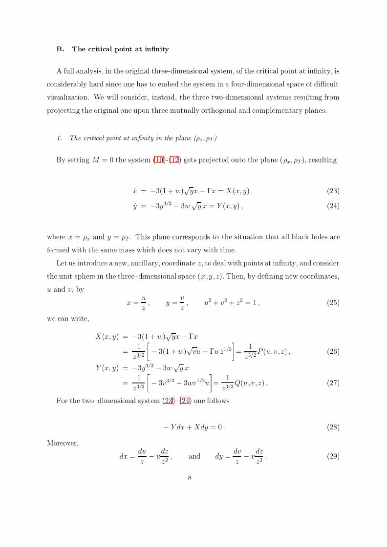
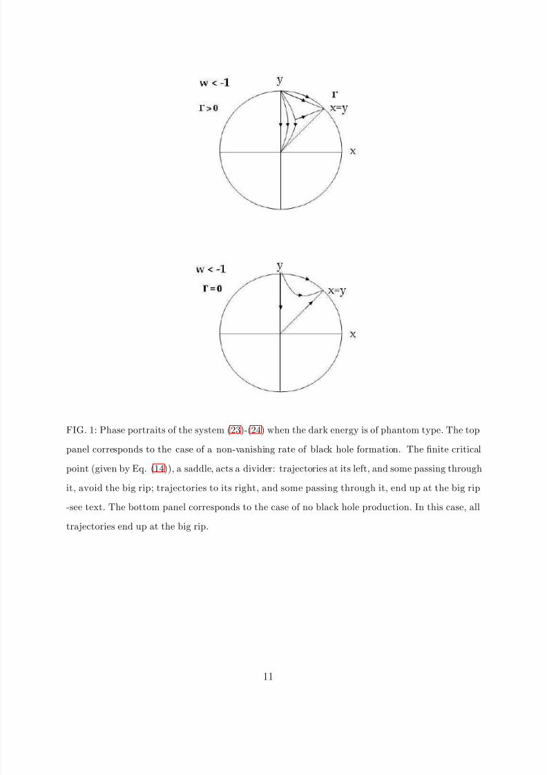
The top panel of Fig. 1 displays the phase portrait. All solutions start from ρT = ρbh → ∞(i.e., the top point on the vertical axis, x = 0). Some of them cannot avoid the big rip

singularity (i.e., the common point to the circle and the straight line x = y). Those solutions

that end up at the center of the circle (the Minkowski state, ρx = ρbh = 0) evade the big

rip. We remark, by passing, that except for the particular case Γ = 0, no solution can go

from the origin to the infinity along the straight line ρx = ρT .

For vanishing Γ (bottom panel of Fig. 1) the finite critical point collapses to the critical

point at the origin, which becomes a saddle point. This represents the usual scenario of a

system composed of pressureless and phantom fluids in which is implicitly assumed that no

black holes are produced.

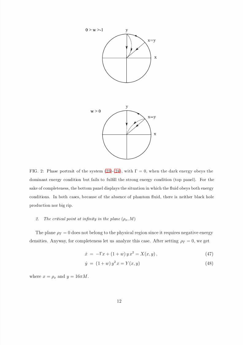
The corresponding phase portraits when the dominant energy condition is satisfied are

shown in the top (0 > w > −1) and bottom (w > 0) panels of Fig. 2.

10



FIG. 1: Phase portraits of the system (23)-(24) when the dark energy is of phantom type. The top

panel corresponds to the case of a non-vanishing rate of black hole formation. The finite critical

point (given by Eq. (14)), a saddle, acts a divider: trajectories at its left, and some passing through

it, avoid the big rip; trajectories to its right, and some passing through it, end up at the big rip

-see text. The bottom panel corresponds to the case of no black hole production. In this case, all

trajectories end up at the big rip.

11



FIG. 2: Phase portrait of the system (23)-(24), with Γ = 0, when the dark energy obeys the

dominant energy condition but fails to fulfill the strong energy condition (top panel). For thesake of completeness, the bottom panel displays the situation in which the fluid obeys both energy

conditions. In both cases, b ecause of the absence of phantom fluid, there is neither black hole

production nor big rip.

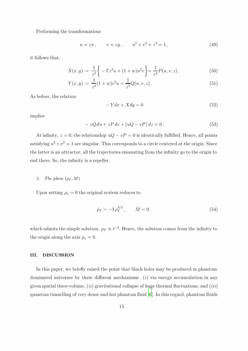
2. The critical point at infinity in the plane (ρx,M )

The plane ρT = 0 does not belong to the physical region since it requires negative energy

densities. Anyway, for completeness let us analyze this case. After setting ρT = 0, we get

x = −Γx + (1 + w) y x2 = X (x, y) , (47)

y = (1 + w) y2 x = Y (x, y) (48)

where x = ρx and y = 16πM .

12



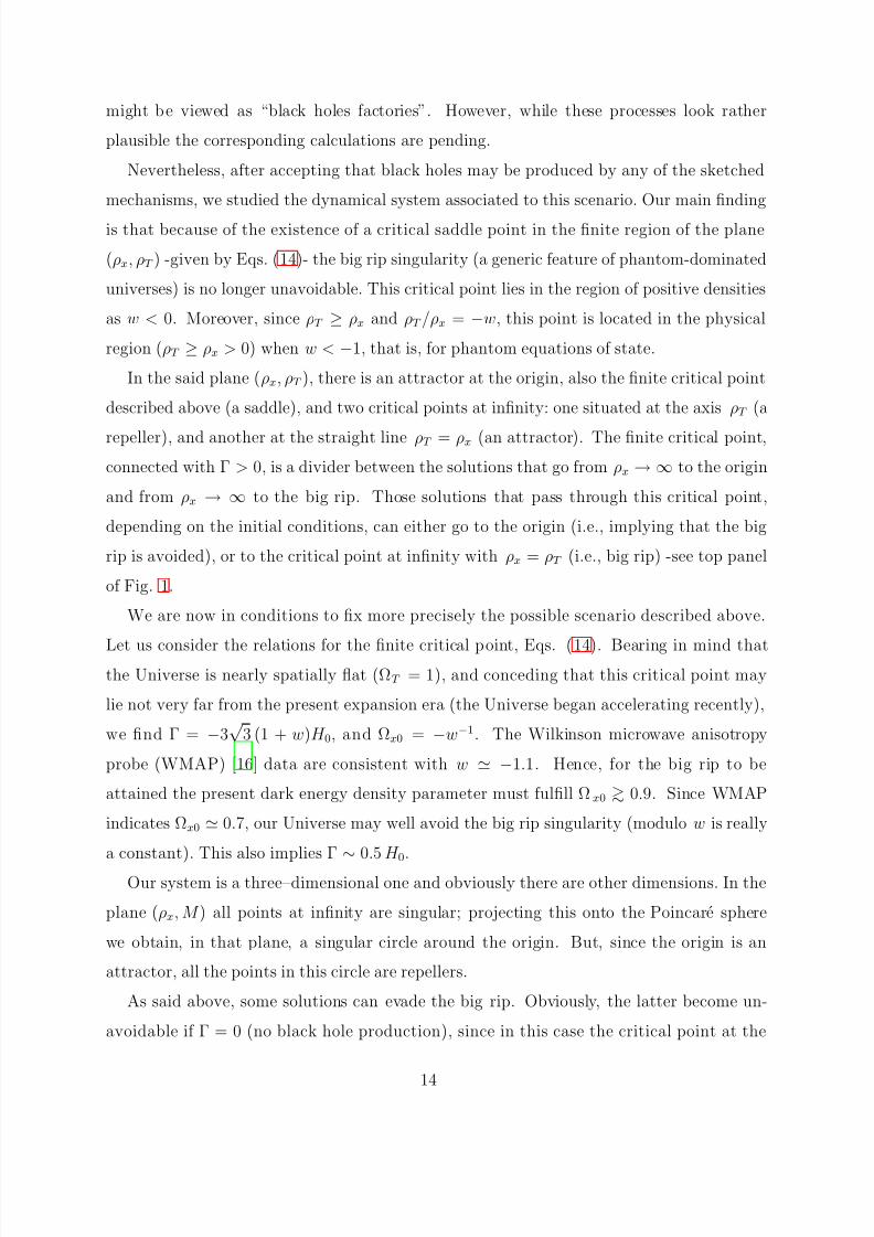
Performing the transformations

u = zx , v = zy , u2 + v2 + z2 = 1 , (49)

it follows that,

X (x, y) =1

z3

− Γz2u + (1 + w)u2v

=

1

z3P (u,v,z) , (50)

Y (x, y) =1

z3(1 + w)v2u =

1

z3Q(u,v,z) . (51)

As before, the relation

− Y dx + Xdy = 0 (52)

implies

− zQdu + zP dv + (uQ − vP ) dz = 0 . (53)

At infinity, z = 0, the relationship uQ − vP = 0 is identically fulfilled. Hence, all points

satisfying u2 + v2 = 1 are singular. This corresponds to a circle centered at the origin. Since

the latter is an attractor, all the trajectories emanating from the infinity go to the origin to

end there. So, the infinity is a repeller.

3. The plane (ρT ,M )

Upon setting ρx = 0 the original system reduces to

ρT = −3 ρ3/2T , M = 0 . (54)

which admits the simple solution, ρT ∝ t−2. Hence, the solution comes from the infinity to

the origin along the axis ρx = 0.

III. DISCUSSION

In this paper, we briefly raised the point that black holes may be produced in phantom

dominated universes by three different mechanisms: (i) via energy accumulation in any

given spatial three-volume, (ii) gravitational collapse of huge thermal fluctuations, and (iii)

quantum tunnelling of very dense and hot phantom fluid [6]. In this regard, phantom fluids

13



might be viewed as “black holes factories”. However, while these processes look rather

plausible the corresponding calculations are pending.

Nevertheless, after accepting that black holes may be produced by any of the sketched

mechanisms, we studied the dynamical system associated to this scenario. Our main finding

is that because of the existence of a critical saddle point in the finite region of the plane

(ρx, ρT ) -given by Eqs. (14)- the big rip singularity (a generic feature of phantom-dominated

universes) is no longer unavoidable. This critical point lies in the region of positive densities

as w < 0. Moreover, since ρT ≥ ρx and ρT /ρx = −w, this point is located in the physical

region (ρT ≥ ρx > 0) when w < −1, that is, for phantom equations of state.

In the said plane (ρx, ρT ), there is an attractor at the origin, also the finite critical point

described above (a saddle), and two critical points at infinity: one situated at the axis ρT (a

repeller), and another at the straight line ρT = ρx (an attractor). The finite critical point,

connected with Γ > 0, is a divider between the solutions that go from ρx → ∞ to the origin

and from ρx → ∞ to the big rip. Those solutions that pass through this critical point,

depending on the initial conditions, can either go to the origin (i.e., implying that the big

rip is avoided), or to the critical point at infinity with ρx = ρT (i.e., big rip) -see top panel

of Fig. 1.

We are now in conditions to fix more precisely the possible scenario described above.

Let us consider the relations for the finite critical point, Eqs. (14). Bearing in mind thatthe Universe is nearly spatially flat (ΩT = 1), and conceding that this critical point may

lie not very far from the present expansion era (the Universe began accelerating recently),

we find Γ = −3√

3 (1 + w)H 0, and Ωx0 = −w−1. The Wilkinson microwave anisotropy

probe (WMAP) [16] data are consistent with w ≃ −1.1. Hence, for the big rip to be

attained the present dark energy density parameter must fulfill Ωx0 >∼ 0.9. Since WMAP

indicates Ωx0 ≃ 0.7, our Universe may well avoid the big rip singularity (modulo w is really

a constant). This also implies Γ∼

0.5 H 0.

Our system is a three–dimensional one and obviously there are other dimensions. In the

plane (ρx, M ) all points at infinity are singular; projecting this onto the Poincare sphere

we obtain, in that plane, a singular circle around the origin. But, since the origin is an

attractor, all the points in this circle are repellers.

As said above, some solutions can evade the big rip. Obviously, the latter become un-

avoidable if Γ = 0 (no black hole production), since in this case the critical point at the

14



finite region coincides with the origin.

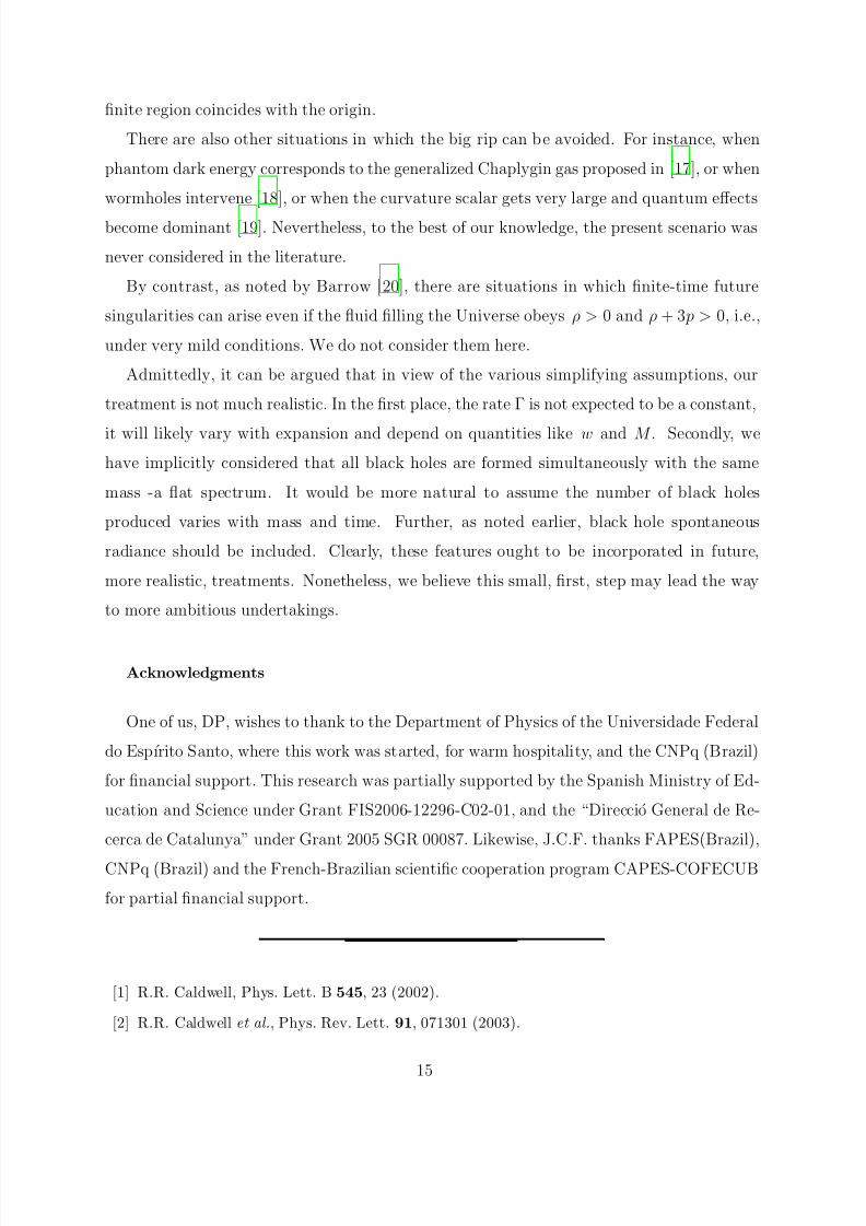
There are also other situations in which the big rip can be avoided. For instance, when

phantom dark energy corresponds to the generalized Chaplygin gas proposed in [17], or when

wormholes intervene [18], or when the curvature scalar gets very large and quantum effects

become dominant [19]. Nevertheless, to the best of our knowledge, the present scenario was

never considered in the literature.

By contrast, as noted by Barrow [20], there are situations in which finite-time future

singularities can arise even if the fluid filling the Universe obeys ρ > 0 and ρ + 3 p > 0, i.e.,

under very mild conditions. We do not consider them here.

Admittedly, it can be argued that in view of the various simplifying assumptions, our

treatment is not much realistic. In the first place, the rate Γ is not expected to be a constant,

it will likely vary with expansion and depend on quantities like w and M . Secondly, we

have implicitly considered that all black holes are formed simultaneously with the same

mass -a flat spectrum. It would be more natural to assume the number of black holes

produced varies with mass and time. Further, as noted earlier, black hole spontaneous

radiance should be included. Clearly, these features ought to be incorporated in future,

more realistic, treatments. Nonetheless, we believe this small, first, step may lead the way

to more ambitious undertakings.

Acknowledgments

One of us, DP, wishes to thank to the Department of Physics of the Universidade Federal

do Espırito Santo, where this work was started, for warm hospitality, and the CNPq (Brazil)

for financial support. This research was partially supported by the Spanish Ministry of Ed-

ucation and Science under Grant FIS2006-12296-C02-01, and the “Direccio General de Re-

cerca de Catalunya” under Grant 2005 SGR 00087. Likewise, J.C.F. thanks FAPES(Brazil),

CNPq (Brazil) and the French-Brazilian scientific cooperation program CAPES-COFECUB

for partial financial support.

[1] R.R. Caldwell, Phys. Lett. B 545, 23 (2002).

[2] R.R. Caldwell et al., Phys. Rev. Lett. 91, 071301 (2003).

15



[3] See any standard textbook on statistical mechanics.

[4] D. Pavon and B. Wang, Gen. Relativ. Grav. 41, 1 (2009), arXiv:0712.0565.

[5] T. Piran and R.M. Wald, Phys. Lett. 90A, 20 (1982).

[6] D. Gross, M.J. Perry, and G.L. Yaffe, Phys. Rev. D 25, 330 (1982).

[7] J.I. Kapusta, Phys. Rev. D 30, 831 (1984).

[8] R.-G. Cai and A. Wang, Phys. Rev. D 73, 063005 (2006).

[9] P.J.E. Peebles and B. Ratra, Rev. Mod. Phys. 75, 559 (2003); K. Hagiwara et al., Phys. Rev.

D 66, 010001 (2002).

[10] E. Babichev et al., Phys. Rev. Lett. 93, 021102 (2004).

[11] S.W. Hawking, Commun Math. Phys. 43, 199 (1975).

[12] D.N. Page, Phys. Rev. D 13, 198 (1976).

[13] G. Sansone and R. Conti, Equazioni Differenziali Non Lineari (Edizioni Cremonese, Rome,

1956).

[14] J.M. Cline, S.-Y. Jeon, and G.D. Moore, Phys. Rev. D 70, 043543.

[15] F. Piazza and S. Tsujikawa, JCAP 07(2004)004.

[16] E. Komatsu et al., “Five-years Wilkinson microwave anisotropy probe (WMAP) observations:

cosmological interpretation”, arXiv:0803.0547.

[17] P.F. Gonzalez-Dıaz, Phys. Rev. D 68, 021303(R) (20063).

[18] J.A. Jimenez Madrid, Phys. Lett. B 634, 106 (2006).

[19] E. Elizalde, S. Nojiri, and S. Odintsov, Phys. Rev. D 70, 043539 (2004).

[20] J.D. Barrow, Class. Quantum Grav. 21, L79 (2004).

http://arxiv.org/abs/0712.0565




Documents

Julio C. Fabris and Diego Pavon- Big rip avoidance via black holes production