Embed Size (px)
Citation preview

Abstract
The linear response function, which describes the change in the electron density induced bya change in the external potential, is the basis for a broad variety of applications. Three ofthese are addressed in the present thesis. In the first part, optical spectra of metallic surfacesare investigated. Quasiparticle energies, i.e., energies required to add or remove an electronfrom a system, are evaluated for selected metals in the second part. The final part of thisthesis is devoted to an improved description of the ground-state electron correlation energy.
In the first part, the linear response function is used to evaluate optical properties ofmetallic surfaces. In recent years, reflectance difference (RD) spectroscopy has provided asensitive experimental method to detect changes in the surface structure and morphology.The interpretation of the resulting spectra, which are linked to the anisotropy of the surfacedielectric tensor, however, is often difficult. In the present thesis, we simulate RD spectra forthe bare, as well as oxygen and carbon monoxide covered, Cu(110) surface, and assign featuresin these spectra to the corresponding optical transitions. A good qualitative agreementbetween our RD spectra and the experimental data is found.
Density functional theory (DFT) gives only access to the ground state energy. Quasi-particle energies should, however, be addressed within many body perturbation theory. Inthe second part of this thesis, we investigate quasiparticle energies for the transition metalsCu, Ag, Fe, and Ni using the Green’s function based GW approximation, where the screenedCoulomb interaction W is linked to the linear response function.
The fundamental limitation of density function theory is the approximation of the exchange-correlation energy. An exact expression for the exchange-correlation energy can be found bythe adiabatic-connection fluctuation-dissipation theorem (ACFDT), linking the linear re-sponse function to the electron correlation energy. This expression has been implementedin the Vienna Ab-initio Simulation Package (VASP). Technical issues and ACFDT resultsobtained for molecules and extended systems, are addressed in the third and last part of thisthesis. Although we make use of the random phase approximation (RPA), we find that thecorrect long-range van der Waals interaction for rare gas solids is reproduced and geometricalproperties for insulators, semiconductors, and metals are in very good agreement with exper-iment. Atomization energies, however, are not significantly improved compared to standardDFT functionals like PBE.
iii

Zusammenfassung
Die Polarisationsfunktion, welche die lineare Dichteanderung durch eine kleine Anderungdes außeren Potentials beschreibt, ist die Grundlage zur Berechnung der unterschiedlichstenphysikalischen Großen. Drei davon werden im Rahmen dieser Dissertation untersucht. Zuerstwerden optische Spektren von metallischen Oberflachen berechnet. Im zweiten Teil werdenfur ausgewahlte Metalle Quasiteilchenenergien berechnet, also diejenigen Energien, welchebenotigt werden, um ein Elektron aus dem System zu entfernen bzw. hinzuzufugen. Derdritte Teil ist schließlich einer verbesserten Beschreibung der elektronischen Korrelationsen-ergie gewidmet.
Im ersten Teil dieser Dissertation werden optische Spektren von metallischen Oberflachenmit Hilfe der Polarisationsfunktion berechnet. In den letzten Jahren erwies sich die reflectancedifference (RD) Spektroskopie als eine experimentelle Methode, die sehr empfindlich aufAnderungen der Oberflachenstruktur reagiert. Eine Interpretation der RD Spektren, welcheauf die Anisotropie des dielektrischen Oberflachentensors zuruckgehen, ist allerdings oftmalsschwierig. Um eine Interpretation zu erleichtern, berechnen wir die RD Spektren sowohl furdie reine, als auch fur die Sauerstoff und Kohlenmonoxid bedeckte Cu(110) Oberflache. Dieberechneten Daten stimmen gut mit den experimentellen Werten uberein und erlauben einegenaue Analyse der Spektren in Bezug auf die zugrunde liegenden optischen Ubergange.
Die Dichtefunktionaltheorie erlaubt allein die Bestimmung der Grundzustandsenergie.Zur Berechnung der Quasiteilchenenergien muss jedoch die Vielteilchenstorungstheorie heran-gezogen werden. Im zweiten Teil dieser Dissertation werden Quasiteilchenenergien fur dieUbergangsmetalle Cu, Ag, Fe und Ni berechnet. Dabei wird die auf der Greensfunktionbasierende GW Naherung verwendet, wobei W, die abgeschirmte Coulombwechselwirkung,von der Polarisationsfunktion abhangt.
Das Fehlen einer exakten Beschreibung der Austausch- und Korrelationsenergie ist diefundamentale Schwachstelle der Dichtefunktionaltheorie. Ein exakter Ausdruck dieser En-ergie kann allerdings mit Hilfe des adiabatic-connection fluctuation-dissipation Theorems(ACFDT) aufgestellt werden. Dabei wird die Korrelationsenergie in Abhangigkeit von derPolarisationsfunktion dargestellt. Routinen zur Berechnung der ACFDT Korrelationsenergiewurden im Vienna Ab-Initio Simulation Package (VASP) implementiert. Details zur Im-plementierung und Ergebnisse fur molekulare und ausgedehnte Systeme werden im drittenund letzten Teil dieser Dissertation behandelt. Obwohl die ACFDT Korrelationsenergie nurnaherungsweise mit Hilfe der random phase approximation (RPA) berechnen wird, wird dielangreichweitige van der Waals Wechselwirkung fur Edelgaskristalle richtig wiedergegeben,und die ACFDT Geometrien von Isolatoren, Halbleitern und Metallen stimmen sehr gut mitden experimentellen Werten uberein.
v

Contents
Abstract iii
I Theory 1
1 Density functional theory 5
1.1 Theorem of Hohenberg-Kohn . . . . . . . . . . . . . . . . . . . . . . . . . . . 5
1.2 Kohn-Sham density functional theory . . . . . . . . . . . . . . . . . . . . . . 5
1.3 DFT in practice . . . . . . . . . . . . . . . . . . . . . . . . . . . . . . . . . . . 8
1.3.1 Plane waves . . . . . . . . . . . . . . . . . . . . . . . . . . . . . . . . . 8
1.3.2 Projector augmented wave method . . . . . . . . . . . . . . . . . . . . 8
2 Optical properties within linear response theory 12
2.1 Time-dependent density functional theory . . . . . . . . . . . . . . . . . . . . 12
2.2 Linear response theory . . . . . . . . . . . . . . . . . . . . . . . . . . . . . . . 13
2.3 Dielectric function - macroscopic continuum considerations . . . . . . . . . . 18
2.4 Macroscopic and microscopic quantities . . . . . . . . . . . . . . . . . . . . . 19
2.5 Longitudinal dielectric function . . . . . . . . . . . . . . . . . . . . . . . . . . 21
2.6 Approximations . . . . . . . . . . . . . . . . . . . . . . . . . . . . . . . . . . . 22
2.7 Calculation of optical properties . . . . . . . . . . . . . . . . . . . . . . . . . 23
2.7.1 PAW response function . . . . . . . . . . . . . . . . . . . . . . . . . . 25
2.7.2 Long-wavelength dielectric function . . . . . . . . . . . . . . . . . . . . 27
2.8 Intraband transitions and the plasma frequency . . . . . . . . . . . . . . . . . 28
2.9 f-sum rule and interband transitions at small energies . . . . . . . . . . . . . 32
3 Total energies from linear response theory 35
3.1 Adiabatic connection dissipation-fluctuation theorem . . . . . . . . . . . . . 36
3.1.1 Adiabatic connection . . . . . . . . . . . . . . . . . . . . . . . . . . . . 36
3.1.2 Fluctuation-dissipation theorem . . . . . . . . . . . . . . . . . . . . . 37
3.2 Random phase approximation . . . . . . . . . . . . . . . . . . . . . . . . . . . 40
3.3 Calculating the RPA correlation energy in practice . . . . . . . . . . . . . . . 41
4 GW quasiparticle energies 44
4.1 The GW approximation . . . . . . . . . . . . . . . . . . . . . . . . . . . . . . 45
4.2 Solving the quasiparticle equation . . . . . . . . . . . . . . . . . . . . . . . . 46
vii
viii CONTENTS
II Reflectance difference spectra 49
5 Calculating reflectance difference spectra 51
5.1 Three-phase model . . . . . . . . . . . . . . . . . . . . . . . . . . . . . . . . . 51
5.2 Calculation of the dielectric function . . . . . . . . . . . . . . . . . . . . . . . 55
6 Optical properties of bulk systems 58
6.1 Plasma frequencies . . . . . . . . . . . . . . . . . . . . . . . . . . . . . . . . . 58
6.2 Dielectric function of bulk copper . . . . . . . . . . . . . . . . . . . . . . . . . 59
6.2.1 Bands . . . . . . . . . . . . . . . . . . . . . . . . . . . . . . . . . . . . 60
6.2.2 k -point convergence . . . . . . . . . . . . . . . . . . . . . . . . . . . . 61
6.2.3 Hilbert transformation . . . . . . . . . . . . . . . . . . . . . . . . . . . 62
6.2.4 Final form of bulk dielectric function and comparison . . . . . . . . . 63
7 Optical calculations for Cu(110) surfaces 66
7.1 Geometry of surfaces . . . . . . . . . . . . . . . . . . . . . . . . . . . . . . . . 66
7.2 Convergence tests . . . . . . . . . . . . . . . . . . . . . . . . . . . . . . . . . . 68
7.2.1 Vacuum . . . . . . . . . . . . . . . . . . . . . . . . . . . . . . . . . . . 69
7.2.2 k-points . . . . . . . . . . . . . . . . . . . . . . . . . . . . . . . . . . . 70
7.2.3 Interband transitions at small frequencies . . . . . . . . . . . . . . . . 70
7.2.4 Number of layers . . . . . . . . . . . . . . . . . . . . . . . . . . . . . . 72
7.3 RDS spectra and interpretation . . . . . . . . . . . . . . . . . . . . . . . . . . 73
7.3.1 Band Structure . . . . . . . . . . . . . . . . . . . . . . . . . . . . . . . 75
7.3.2 Reflectance difference spectra . . . . . . . . . . . . . . . . . . . . . . . 78
8 Conclusions and Summary 83
III GW calculations 85
9 Quasiparticle energies for metals 86
9.1 Noble metals - Cu and Ag . . . . . . . . . . . . . . . . . . . . . . . . . . . . . 86
9.2 Ferromagnets: Fe, Ni . . . . . . . . . . . . . . . . . . . . . . . . . . . . . . . . 92
IV Total energies from ACFDT 99
10 Implementation of the ACFDT routines 101
10.1 Dependence on dimension of the response function . . . . . . . . . . . . . . . 102
10.2 Frequency integration . . . . . . . . . . . . . . . . . . . . . . . . . . . . . . . 106
10.3 k-point convergence and Γ-point correction for metals . . . . . . . . . . . . . 109
10.3.1 Γ-point corrections: Technical details . . . . . . . . . . . . . . . . . . . 111
11 Application of the ACFDT 114
11.1 Molecules - H2, O2, N2 . . . . . . . . . . . . . . . . . . . . . . . . . . . . . . . 114
11.2 Rare-gas solids - Ne, Ar, Kr . . . . . . . . . . . . . . . . . . . . . . . . . . . . 117
11.3 Homogenous electron gas . . . . . . . . . . . . . . . . . . . . . . . . . . . . . 122
CONTENTS ix
11.4 Metals - Na, Al, Cu, Rh, Pd . . . . . . . . . . . . . . . . . . . . . . . . . . . . 12511.5 Solids . . . . . . . . . . . . . . . . . . . . . . . . . . . . . . . . . . . . . . . . 130
11.5.1 Lattice constants and bulk moduli . . . . . . . . . . . . . . . . . . . . 13311.5.2 Atomization energies . . . . . . . . . . . . . . . . . . . . . . . . . . . . 143
12 Conclusions and Summary 150
Bibliography 153
List of Publications 161
Acknowledgments 163
Curriculum vitae 165


Part I
Theory
1
2
The non-relativistic Schrodinger equation for N electrons moving in an external potentialvext considering decoupling of ionic and electronic degrees of freedom (Born-Oppenheimerapproximation) is given as:
− h2
2m
N∑
i=1
∇2ri
+1
2
∑
i6=j
e2
|ri − rj|+∑
i
vext(xi, R) + Eion(R)
Ψ(x) =
= E(R)Ψ(x), (1)
where the electron energy is parametric depending on the ionic coordinates R and x = (r, s)denotes both electron positions and spins. In the further discussion we will consider ”spinless”electrons. Furthermore, we neglect the Eion term, which describes the electrostatic interactionbetween the positive ions and which is constant for a fixed ionic configuration. The electronicHamiltonian then reads:
H = − h2
2m
N∑i=1∇2
ri+ 1
2
∑i6=j
e2
|ri−rj |+
∑ivext(ri)
= T + Vee + Vext.
(2)
Instead of solving this eigenvalue problem, the ground state energy EGS can be obtained byminimizing
〈Ψ|H |Ψ〉 under the constraint 〈Ψ|Ψ〉 = 1. (3)
Such a minimization over the space of many-electron wavefunctions
Ψ(r) = Ψ(r1, r2, . . . , rN ) (4)
is only possible for system containing a few electrons. For a larger number of electrons, thecomplexity of the electron problem becomes intractable due to the large number of degrees offreedom involved. It is therefore desirable to search for quantities of lower dimension whichdefine the ground state energy uniquely. One possible quantity is the electron density
n(r) = N
∫d3r2 d
3r3 . . . d3rN Ψ∗(r, r2, . . . , rN )Ψ(r, r2, . . . , rN ) (5)
which can also be written as
n(r) = 〈Ψ|n(r)|Ψ〉 with the density operator n(r) =N∑
i
δ(r− ri). (6)
The density n(r) describes the probability to find an electron at place r, if all other electronsare located at any place, and it, therefore, contains much less information than the fullmany-body wavefunction Ψ(r). It is not straightforward that the ground state energy canbe expressed as a quantity solely depending on the density. This can only be the case ifdifferent external potentials inevitably result in different densities for a N electron system.The validity of this requirement has been first proven by Hohenberg and Kohn [1] in 1964.A more general proof was provided by Levy in 1979 [2]. On these foundations all methodssummarized under the name ”density functional theories” are based. We will later come back
3
to the theorem of Hohenberg and Kohn and to its practical realization as proposed by Kohnand Sham [3].
But also for the straightforward evaluation of the ground state energy, the entire many-body wavefunction is not required. Three parts contribute to the electronic energy
E = 〈Ψ|T |Ψ〉 + 〈Ψ|Vee|Ψ〉 + 〈Ψ|Vext|Ψ〉kinetic energy e-e interaction external potential.
(7)
The energy resulting from the external potential, 〈Ψ|Vext|Ψ〉, is given as
〈Ψ|Vext|Ψ〉 =
N∑
i=1
∫d3r1 . . . d
3rN Ψ∗(r1, r2, . . . , rN ) vext(ri)Ψ(r1, r2, . . . , rN ) =
= N
∫d3r d3r2 . . . d
3rN Ψ∗(r, r2, . . . , rN ) vext(r)Ψ(r, r2, . . . , rN ) =
=
∫d3r vext(r)n(r) (8)
and is consequently only depending on the electron density n(r). The kinetic energy is alsoa ”one-electron” quantity:
〈Ψ|T |Ψ〉 = −h2
2m
N∑
i=1
∫d3r1d
3r2 . . . d3rN Ψ∗(r1, r2, . . . , rN )∇2
riΨ(r1, r2, . . . , rN ) =
= −Nh2
2m
∫d3r′ d3r d3r2 . . . d
3rN δ(r − r′)Ψ∗(r′, r2, . . . , rN )∇2r Ψ(r, r2, . . . , rN )
= −h2
2m
∫d3r′d3r δ(r − r′)∇2
r γ(r, r′) = −
h2
2m
∫d3r
[∇2
r γ(r, r′)]r′=r
(9)
where γ(r, r′) is the one-particle density matrix:
γ(r, r′) = N
∫d3r2 d
3r3 . . . d3rN Ψ∗(r′, r2, . . . , rN )Ψ(r, r2, . . . , rN ). (10)
The remaining term, the electron-electron interaction, links the coordinates of every twoelectrons:
〈Ψ|Vee|Ψ〉 =1
2
∑
i6=j
∫d3r1d
3r2 . . . d3rN Ψ∗(r1, r2, . . . , rN )
e2
|ri − rj |Ψ(r1, r2, . . . , rN ) =
=N(N − 1)
2
∫d3r1d
3r2e2
|r1 − r2|
∫d3r3 . . . d
3rN Ψ∗(r1, r2, . . . , rN )Ψ(r1, r2, . . . , rN ) =
=e2
2
∫d3r1d
3r2n2(r1, r2)
|r1 − r2|(11)
where n2(r1, r2) is the pair density which can be defined as the trace of the two-electrondensity matrix, n2(r1, r2) = Γ(r1, r2; r1, r2):
Γ(r1, r2; r′1, r
′2) = N(N − 1)
∫d3r3 . . . d
3rNΨ∗(r1, r2, . . . , rN )Ψ(r′1, r′2, . . . , rN ). (12)
4
If the classical electrostatic energy (Hartree-Term)
EH =e2
2
∫d3r d3r′
n(r)n(r′)
|r− r′|(13)
is subtracted from 〈Ψ|Vee|Ψ〉 and the exchange-correlation hole nxc(r1, r2) is introduced
nxc(r1, r2) =n2(r1, r2)
n(r1)− n(r2) (14)
the total energy of the electronic system reads
E = −h2
2m
∫d3r
[∇2
rγ(r′, r)]r′=r
+e2
2
∫d3r d3r′
n(r)n(r′)
|r− r′|+
+e2
2
∫d3r d3r′
n(r)nxc(r, r′)
|r− r′|+
∫d3r vext(r)n(r). (15)
This suggests that there should be ways to calculate the energy without considering thewhole many-body wavefunction. Besides the already mentioned density functional theories(DFT), methods based on the pair density n2(r1, r2) and the two-electron density matrixΓ(r1, r2; r
′1, r
′2) have been considered. Whereas in DFT the exact density dependent form for
the kinetic energy term and the electron-electron interaction is not known, theories basedon the pair density lack an exact expression for the kinetic energy term only (see e.g., [4]).Introducing the two-electron density matrix Γ(r1, r2; r
′1, r
′2) lifts this problem, but the N -
representability problem (which conditions must a two-electron density matrix obey to bederived from a many-body wavefunction) comes to the fore (e.g., [5]).
Chapter 1
Density functional theory
1.1 Theorem of Hohenberg-Kohn
The term density functional theory (DFT) refers to all methods that express the ground-stateenergy as a functional of the electronic density n(r). The validity of such an approach wasfirst proven by Hohenberg and Kohn in 1964 [1] and later generalized by Levy [2]. Hohenbergand Kohn introduced the energy functional
EHK [n] := F [n] +
∫d3r n(r) v(r) F [n] := min
Ψ→n〈Ψ|T + Vee|Ψ〉 (1.1)
and proved that
1. F [n] is a unique functional of the density n(r) i.e., for an N electron system, there donot exist two ground state wavefunctions Ψ1 6= Ψ2 (potentials v1 6= v2) resulting in thesame density n(r).
2.EHK [n] ≥ EGS
The energy functional EHK obeys a variational principle and always results in energieslarger or equal to the ground state energy EGS .
3.EHK [nGS] = EGS
The energy functional EHK reaches the ground state energy at the ground state densitynGS .
1.2 Kohn-Sham density functional theory
The Hohenberg-Kohn (HK) theorem provides a theoretical justification for the constructionof an energy functional that depends on the electron density only, but it does not provide aconcrete expression for the energy functional F [n] = minΨ→n〈Ψ|T+Vee|Ψ〉. Actually, densityfunctionals as the Thomas-Fermi functional [6, 7] have been used before the HK theorem.In the Thomas-Fermi functional three terms are considered: the classical electron-electron
5
6 CHAPTER 1. DENSITY FUNCTIONAL THEORY
repulsion (Hartree term), the energy resulting from the external potential, and a kineticenergy term, which is approximated in a local density approximation by the kinetic energyof the homogenous electron gas ∝ n1/3. This approximation allowed an exact mathematicaltreatment of the resulting integral equation, but it could also be shown [8, 9] that binding ofatoms to form molecules and solids can not be described within Thomas-Fermi theory.
In 1965, Kohn and Sham [3] proposed a different approximation for the functional F [n]that maps the problem of a system of interacting particles onto a system of independentelectrons with the same density n(r) moving in an effective local potential that mimicsthe influence of the other electrons. The energy of an electron system [Eq. (7)] can bereformulated to
E[n] = Ts[n] + EH [n] + Exc[n] + Eext[n] with
Exc[n] := 〈ΨMB|T |ΨMB〉 − Ts[n] + 〈ΨMB |Vee|ΨMB〉 − EH [n]. (1.2)
The wavefunction of the true, interacting, system is thereby denoted as ΨMB, whereas thewavefunction of the reference system of independent particles is a Slater determinant builtfrom one-electron wavefunctions ψn. The independent particle kinetic energy Ts[n] =−h2/2m
∑n(occ)〈ψn|∇2|ψn〉 thereby depends only implicitely on the electron density
n(r) = 2∑
n(occ)
|ψn(r)|2 (1.3)
via the one-electron wavefunctions ψn. By introducing the Hartree potential
vH [n](r) = e2∫d3r′
n(r′)
|r− r′|(1.4)
and the (abstract) µxc[n](r) energy density per particle, the energy can also be written as
E[n] = Ts[n] +
∫d3r n(r)
[1
2vH [n](r) + µxc[n](r) + vext(r)
]
︸ ︷︷ ︸(1.5)
vKS[n](r).
The ground state energy EGS can be found by minimizing Eq. (1.5) with respect to thedensity n(r) or solving the so called Kohn-Sham equations:
(−h2
2m∇2 + vKS[n](r) +
∫d3r n(r)
δvKS [n]
δn(r′)
)ψn = ǫnψn
m (1.6)(−h2
2m∇2 + vH [n](r) + vxc[n](r) + vext(r)︸ ︷︷ ︸
)ψn = ǫnψn,
veff [n](r)
where the exchange correlation potential vxc[n](r) is defined as:
vxc[n](r) =δExc[n]
δn(r). (1.7)
1.2. KOHN-SHAM DENSITY FUNCTIONAL THEORY 7
Due to the dependence of the KS Hamiltonian on the density and thus on the wavefunc-tions themselves, Eq. (1.6) have to be solved selfconsistently. By introducing the occupationfunction fn,
fn = 1 if state n is occupied
0 if state n is unoccupied,(1.8)
the ground state energy EGS can be written as
EGS = 2∑
n
fnǫn − EH [nGS]−
∫d3r nGS(r) vxc[nGS ](r) + Exc[nGS ] (1.9)
with the ground state density
nGS(r) = 2∑
n
fn|ψn(r)|2 (1.10)
given by the wavefunctions solving Eq. (1.6).
By applying the Kohn-Sham density functional theory, the ground state energy andground state density can thus be calculated by solving a set of one-electron Schrodinger equa-tions. However, the exchange-correlation energy functional Exc[n] or the exchange-correlationpotential, respectively, have to be approximated. The earliest approach has been the so calledlocal density approximation (LDA) [3], which assumes that the exchange-correlation energycan be locally approximated by the exchange-correlation energy density of the homogeneouselectron gas ǫunif
xc [n] (energy per particle) at the respective density:
Exc[n(r)] =
∫d3r n(r) ǫunif
xc [n]. (1.11)
The exchange-correlation energy of the homogenous electron gas has been calculated byCeperley and Alder for a set of densities using quantum Monte Carlo methods [10]. Theparametrisation of these energies suggested by Perdew and Wang [11] will be used in thefollowing.
The LDA assumes that the exchange correlation energy of an inhomogenous system canbe approximated at each point by the energy of a homogenous electron gas. In the moresophisticated generalized gradient approximation (GGA) not only the density but also thevariation of the density, the density gradient, is considered for the calculation of the exchange-correlation energy
EGGAxc [n] =
∫d3r f(n,∇n). (1.12)
GGA functionals can be either constructed as to fulfill (some) exact conditions, or by fittingto energies calculated on a higher level of theory or experimental values. The GGA introducedby Perdew, Burke, and Ernzerhof (PBE) [12], which is used in the present work, belongs tothe first class of GGAs.
8 CHAPTER 1. DENSITY FUNCTIONAL THEORY
1.3 DFT in practice
In the present section, we will briefly describe how the Kohn-Sham equations are solved inthe Vienna ab-initio simulation package (VASP) used throughout this thesis. More detailsabout the plane wave approach can be found e.g., in the review of Payne et al. [13]. ThePAW method is discussed in Ref. [14] and with respect to the VASP code in Ref. [15].
1.3.1 Plane waves
For the actual solution of the Kohn-Sham equations the wavefunctions are usually expandedin a basis set. In our case, this basis set consists of plane waves. For a periodic system,each wavefunction can be written as a Bloch function ψnk(r) = unk(r) eikr where unk(r)exhibits the same periodicity as the system itself and can therefore be expanded with respectto reciprocal lattice vectors G: unk(r) =
∑G cnk(G) eiGr. The wave vector k lies within the
first Brillouin zone. In practice, a finite grid of k-points, in the form of e.g., a Monkhorst-Packgrid [16], is used for the sampling of the Brillouin zone. Applying the concept of periodicityon the Kohn-Sham equations, they split up into Nk (number of k-points) equations, whichcan be solved separately. For finite or aperiodic systems the concept of periodicity is certainlyartificial. But these systems can be treated within the supercell approach where the respectivesystems are placed in large three-dimensional supercells in order to avoid interactions betweenthe repeated images.
Due to the plane wave approach it is costly to describe strongly localized electrons withrapid oscillations, such as electrons close to the core. They require a large number of planewaves in the expansion of the cell periodic function
unk(r) =
|k+G|2/2<Ecut∑
G
cnk(G) eiGr (1.13)
and consequently a large value for the plane wave energy cutoff Ecut, slowing the DFTcalculations drastically. To circumvent this problem, we do not consider the KS equations forenergetically deeper lying electrons, core electrons, (frozen core approximation) and describethe remaining electrons, valence electrons, within the projector augmented-wave method(PAW) [14, 15].
1.3.2 Projector augmented wave method
The main idea of the PAW method is to divide space into two regions: the augmentationregion Ωa (atom-centered spheres) and the interstitional region ΩI between these spheres.Within the augmentation regions Ωa the all-electron (AE) wavefunction |ψnk〉 of state n andk-point k can be expanded with respect to a set for AE partial-waves |φi〉
|ψnk〉 =∑
i
ci,nk |φi〉 in Ωa. (1.14)
The AE partial waves are solutions to the all-electron KS-DFT equation for a sphericalreference atom of type N situated at the atomic site R for different angular momentumnumbers L = l,m and reference energies ǫαl. The index i is an abbreviation for R, N , L,
1.3. DFT IN PRACTICE 9
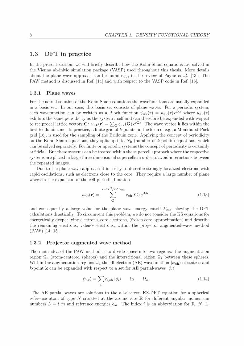
+ −
AE PS AE on−site PS on−site
Figure 1.1: Wavefunction/density representation in the projector augmented-wave method.
and the index of the reference energy α. The radial part of the solution can be split off andby means of the spherical harmonics Ylm the AE partial-wave can be written as:
〈r|φi〉 = φi(r) = Ylm( r−R)φNlα(|r−R|). (1.15)
Additionally pseudo (PS) partial waves
〈r|φi〉 = φi(r) = Ylm( r−R) φNlα(|r−R|) (1.16)
are generated, which are smooth functions inside the augmentation-spheres and match theAE partial-waves outside Ωa. This is achieved by expanding φNlα(r) with respect to Besselfunctions jl(qr). For more details see [15] Sec. IV B.
Pseudo wavefunctions |ψnk〉 represented using plane waves are finally introduced. Theseare defined as:
|ψnk〉 =∑
i ci,nk |φi〉 in Ωa
|ψnk〉 = |ψnk〉 inΩI .
(1.17)
The representation of the PS wavefunction |ψnk〉 requires only a modest number of planewaves because the AE partial waves |φi〉 with their rapid oscillations near the atomic core re-gion Ωa are replaced by the smooth PS partial waves |φi〉. By introducing projector functions|pi〉 that are dual to the PS partial waves
〈pi|φj〉 = δij , (1.18)
the coefficients ci,nk can be obtained by
〈pi|ψnk〉 =∑
j
cj,nk 〈pi|φj〉 = ci,nk. (1.19)
Combining Eq. (1.14) and Eq. (1.17), the AE wavefunction |ψnk〉 can be written as:
|ψnk〉 = |ψnk〉+∑
i
〈pi|ψnk〉 |φi〉 −∑
i
〈pi|ψnk〉 |φi〉. (1.20)
10 CHAPTER 1. DENSITY FUNCTIONAL THEORY
This splitting of the AE wavefunction is visualized schematically in Fig. 1.1. The AE wave-function |ψnk〉 with large oscillations (slashed spheres) in Ωa is described by a PS wavefunc-tion |ψnk〉 which is smooth in the entire space and corresponds to the AE wavefunction in theinterstitional region ΩI . It is expanded with respect to a plane-wave basis set. To correct forthe PS error an AE on-site term is added inside the augmentation regions Ωa. Contributionsalready accounted for by the PS wavefunctions are finally expressed by PS partial waves andsubtracted. The same separation as for the wavefunctions approximately holds also for thedensity
n(r) =∑
nk
fnk 〈ψnk|r〉 〈r|ψnk〉, (1.21)
which can be written as
n(r) =∑
nk
fnk 〈ψnk|r〉 〈r|ψnk〉 +∑
ij
ρij〈φi|r〉 〈r|φj〉 −∑
ij
ρij〈φi|r〉 〈r|φj〉 =
= n(r) + n1(r) − n1(r)
with
ρij =∑
nk
fnk 〈ψnk|pi〉 〈pj |ψnk〉 =∑
nk
fnk c∗i,nk cj,nk. (1.22)
The pseudo density n(r) is thereby described on a regular grid spanning the entire supercellvolume. A Fast Fourier Transform is used to switch between the plane wave coefficient ci,nk
and the real space representation of the PS wavefunction ψnk(r). The plane wave grid onwhich the PS wavefunction is thereby evaluated in real space is closely related to the regulargrid. The on-site PS and AE densities n1(r) and n1(r) are represented on radial grids in theaugmentation spheres Ωa centered around the ions. The separation into terms arising fromcontributions represented on regular and radial grids holds (approximately) also for the totalenergy, if one introduces the compensation charge density n(r) (see [15] Sec. II B, C). Thecompensation charge density n is added to the PS charge density n(r) in order to restore theAE monopole and multipoles up to a certain angular momentum number L. Consequently,n has to fulfill the requirement:
∫
Ωa(Ri)
(n1 − n1 − n
)|r−Ri|
l Y ∗L ( r−Ri) d
3r = 0. (1.23)
The compensation charge n should therefore reproduce the multipoles of the augmentationcharge density Qij
n1(r)− n1(r) =∑
ij
ρij Qij(r) Qij(r) = φ∗i (r)φj(r)− φ∗i (r)φj(r), (1.24)
but at the same time its shape has to be smoother than the one of the fast varying Qij(r),because it has to be represented on a regular grid in order to add it to the PS charge density.By introducing the moments of the augmentation charge
qLij =
∫
Ωa(Ri)Qij(r) |r−Ri|
l Y ∗L ( r−Ri) d
3r, (1.25)
1.3. DFT IN PRACTICE 11
the compensation charge density can be expressed as
n =∑
ij
ρij QLij(r) QL
ij(r) = qLij gl(|r−R|)YL( r−R), (1.26)
where gl(|r−R|) is a smooth function which a l-moment of one. For more details about theconstruction of gl(|r−R|) see [15] Sec. IV D.
Chapter 2
Optical properties within linearresponse theory
2.1 Time-dependent density functional theory
Time-dependent density functional theory (TDDFT) aims at mapping the time-dependentSchrodinger equation
i∂
∂tΨ(t) = HΨ(t) (2.1)
onto an effective one-electron problem, as density functional theory does for the staticSchrodinger equation. In 1984, Runge and Gross [17] proved that, for a given initial state, aone-to-one correspondence exists between the time-dependent density n(r, t) and the time-dependent external potential vext(r, t). The Runge-Gross theorem is the fundament ofTDDFT as the Hohenberg-Kohn theorem [1] is the justification for (static) DFT. Analo-gous to static DFT, time-dependent Kohn-Sham equations can be introduced, which mapthe problem of interacting electrons moving in a time-dependent external potential vext ontoa system of independent electrons moving in a time-dependent effective potential veff . Theresulting time-dependent Kohn-Sham equations take the form:
i∂ψn(r, t)
∂t=
[−h2
2m∇2 + veff [n](r, t)
]ψn(r, t) n(r, t) = 2
∑
n(occ)
|ψn(r, t)|2. (2.2)
The effective potential veff can be split into the external potential, the (via the density)time-dependent Hartree potential, and the exchange-correlation potential
veff [n](r, t) = vext(r, t) + vH [n](r, t) + vxc[n](r, t). (2.3)
The time-dependent Hartree potential is defined as
vH [n](r, t) = e2∫d3r′
n(r′, t)
|r− r′|. (2.4)
The time-dependent exchange-correlation potential vxc is a quantity that depends on thehistory of the density n(r, t) and the initial interacting many-electron and Kohn-Sham wave-functions. In the following we will only consider the influence of a weak external potential
12
2.2. LINEAR RESPONSE THEORY 13
(linear response regime), but a detailed overview on TDDFT and various applications canbe found in Ref. [18].
2.2 Linear response theory
Both in the calculation of the reflectance difference spectra (part II of this thesis) and inthe improved description of the DFT exchange-correlation energy (part IV) we have to eval-uate the response of the material to an external perturbation. If this perturbation is weakcompared to the internal electric fields caused by the ions, as usually in spectroscopic exper-iments, the induced change in the density can be described within perturbation theory aslinearly dependent on the applied perturbation.
The key quantity of linear response theory is the response function χ(r, r′, t− t′), whichdescribes the change of the density δn at (r, t) if the external potential undergoes a smallchange δvext at (r′, t′).
δn(r, t) =
∫dt′∫d3r′ χ(r, r′, t− t′) δvext(r
′, t′) (2.5)
χ(r, r′, t− t′) =δn(r, t)
δvext(r′, t′). (2.6)
Within the Kohn-Sham formulation it is easier to calculate the Kohn-Sham (KS) responsefunction χKS(r, r′, t − t′), which describes the response of the KS system to a small changeof the effective Kohn-Sham potential veff [n]:
δn(r, t) =
∫dt′∫d3r′ χKS(r, r′, t− t′) δveff (r′, t′) (2.7)
χKS(r, r′, t− t′) =δn(r, t)
δveff (r′, t′). (2.8)
The requirement that the change of the density δn(r, t) is the same in both descriptions linksthe response function of the interacting system χ(r, r′, t − t′) to the KS response functionχKS(r, r′, t − t′). In order to write this relation explicitely, we introduce the exchange-correlation kernel fxc
vxc[nGS + δn](r, t) = vxc[nGS](r) +
∫dt′∫d3r′ fxc[nGS ](r, r′, t− t′) δn(r′, t′) (2.9)
fxc[nGS](r, r′, t− t′) =δvxc(r, t)
δn(r′, t′)
∣∣∣n=nGS
, (2.10)
which is defined as the derivative of the time-dependent exchange-correlation potential withrespect to the time-dependent density evaluated at the ground state density nGS. By requir-ing that Eq. (2.5) and Eq. (2.7) are the same, the link between χ and χKS is given as [seeEq. (2.3)]:∫dt′∫d3r′ χ(r, r′, t− t′) δvext(r
′, t′) =
=
∫dt′∫d3r′ χKS(r, r′, t− t′)
δvext(r
′, t′) + δvH(r′, t′) + δvxc(r′, t′)
. (2.11)
14 CHAPTER 2. OPTICAL PROPERTIES WITHIN LINEAR RESPONSE THEORY
Applying the chain rule on δvH and δvxc,
δvH(r′, t′) =
∫dt1 dt2
∫d3r1 d
3r2δvH(r′, t′)
δn(r1, t1)
δn(r1, t1)
δvext(r2, t2)δvext(r2, t2) (2.12)
=
∫dt1 dt2
∫d3r1 d
3r21
|r1 − r′|χ(r1, r2, t1 − t2) δvext(r2, t2)
δvxc(r′, t′) =
∫dt1 dt2
∫d3r1 d
3r2δvxc(r
′, t′)
δn(r1, t1)
δn(r1, t1)
δvext(r2, t2)δvext(r2, t2) = (2.13)
=
∫dt1 dt2
∫d3r1 d
3r2 fxc(r′, r1, t
′ − t1)χ(r1, r2, t1 − t2) δvext(r2, t2),
changing the names of the integration variables, and going to frequency space finally leadsto the relationship:
χ(r, r′, ω) = χKS(r, r′, ω) +
+
∫d3r1 d
3r2 χKS(r, r1, ω)
(e2
|r1 − r2|+ fxc(r1, r2, ω)
)χ(r2, r
′, ω). (2.14)
This relationship is generally referred to as Dyson equation. For the evaluation of the responsefunction of an interacting electron system the response function of the respective Kohn-Sham system is calculated and afterwards the interacting response function is estimatedby applying the Dyson equation with some approximated exchange-correlation kernel. Theeasiest approximation for fxc is to ignore the effect of the exchange-correlation at all (fxc = 0).This simplification is called random phase approximation (RPA) or Hartree approximation(because only the Hartree term δvH contributes).
Following the derivation of Pines and Noziere [19] (see also [20]), an explicit formula for theresponse to an external (time-dependent) potential δv(r, t), leading to a small perturbationin the Hamiltonian
δH(t) = eηtN∑
i=1
δv(ri, t) 0 < η ≪ 1, (2.15)
can be found. The factor eηt is introduced to guarantee an adiabatic, slow switching from theunperturbed Hamiltonian for t → −∞ ( eηt = 0) to 1 for t = 0. With the density operatorn(r) =
∑Ni=1 δ(r− ri), the perturbation can be written in frequency space as
δH(t) =
∫d3r
∫dω
2πe−iωt δv(r, ω) n(r) ω := ω + iη. (2.16)
If |Ψ00〉 and E0
0 are the ground state wavefunction and ground state energy of the stationarySchrodinger equation H0|Ψ0
j〉 = Ej|Ψ0j 〉, where H0 is the unperturbed Hamiltonian, the
solution of the (unperturbed) time-dependent Schrodinger equation is given as
|Ψ0(t)〉 = e−iE0t |Ψ00〉. (2.17)
Introducing the time-dependent perturbation δH(t), the Schrodinger equation reads:
i∂|Ψ(t)〉
∂t=(H0 + δH(t)
)|Ψ(t)〉. (2.18)
2.2. LINEAR RESPONSE THEORY 15
Within first-order perturbation theory, |Ψ(t)〉 can be written as
|Ψ(t)〉 = e−iE0t |Ψ00〉︸ ︷︷ ︸+
∑
j 6=0
aj(t) e−iEjt |Ψ0
j〉. (2.19)
|Ψ0(t)〉
It can be described as the unperturbed time-dependent solution |Ψ0(t)〉 plus an admix-ture of components resulting from excited states of the unperturbed Schrodinger equatione−iEjt |Ψ0
j 〉. The time-dependent coefficients are given by:
aj(t) = −i
∫ t
−∞dt′ eiω0j t′ 〈Ψ0
j |δH(t′)|Ψ00〉 =
= −i
∫d3r′
∫dω
2π
∫ t
−∞dt′ ei(ω0j−ω)t′ δv(r′, ω)〈Ψ0
j |n(r′)|Ψ00〉 = (2.20)
= −
∫d3r′
∫dω
2πδv(r′, ω) 〈Ψ0
j |n(r′)|Ψ00〉ei(ω0j−ω)t
ω0j − ω,
where ω0j denotes the difference between the energy of an exited state and the ground state,ω0j = Ej −E0. The change of the density resulting from the time-dependent perturbation
nind(r, t) = δn(r, t) = 〈Ψ(t)|n(r)|Ψ(t)〉 − 〈Ψ0(t)|n(r)|Ψ0(t)〉 (2.21)
can be written as
nind(r, t) =∑
j 6=0
[aj(t) 〈Ψ
00|n(r)|Ψ0
j 〉 e−iω0j t + a∗j(t) 〈Ψ
0j |n(r)|Ψ0
0 〉eiω0jt
]=(2.20)
= −
∫d3r′
∫dω
2πδv(r′, ω) e−iωt ×
×∑
j 6=0
( 〈Ψ0j |n(r′)|Ψ0
0〉 〈Ψ00|n(r)|Ψ0
j 〉
ω0j − ω+〈Ψ0
0|n(r′)|Ψ0j〉 〈Ψ
0j |n(r)|Ψ0
0〉
ω0j + ω
), (2.22)
if terms proportional to the square of |Ψ(t)〉 − |Ψ0(t)〉 are neglected. The induced density infrequency space becomes
nind(r, ω) = −
∫d3r′ δv(r′, ω) ×
×∑
j 6=0
( 〈Ψ0j |n(r′)|Ψ0
0〉〈Ψ00|n(r)|Ψ0
j 〉
ω0j − ω+〈Ψ0
0|n(r′)|Ψ0j〉〈Ψ
0j |n(r)|Ψ0
0〉
ω0j + ω
). (2.23)
The change of the density nind = δn with respect to the change of the potential δv inducedby the external perturbation is exactly the response function
δn(r, ω)
δv(r′, ω)= χ(r, r′, ω) =
= −∑
j 6=0
(〈Ψ0j |n(r′)|Ψ0
0〉〈Ψ00|n(r)|Ψ0
j 〉
ω0j − ω+〈Ψ0
0|n(r′)|Ψ0j 〉〈Ψ
0j |n(r)|Ψ0
0〉
ω0j + ω
). (2.24)
16 CHAPTER 2. OPTICAL PROPERTIES WITHIN LINEAR RESPONSE THEORY
For a system of non-interacting electrons (and the KS system can be considered as a systemof independent electrons moving in an effective potential), the ground state wavefunction Ψ0
0
can be written as a product of one-particle wavefunctions ψn (or as a Slater determinant,respectively):
Ψ00(r1, r2, . . . , rN/2) = ψ1(r1)ψ2(r2) . . . ψn(ri) . . . ψN/2(rN/2), (2.25)
where the functions ψ1 . . . ψN/2 are the N/2 lowest solutions of the one-particle Schrodingerequation (or KS equation). Orthonormality holds for the one-particle wavefunctions ψn. Anexcited state of the system can be generated by ”moving” one electron from an occupiedstate to an unoccupied state generating the excited wavefunction
Ψ0j(r1, r2, . . . , rN/2) = ψ1(r1)ψ2(r2) . . . ψm(ri) . . . ψN/2(rN/2) m > N/2. (2.26)
For the system of independent electrons, the expression 〈Ψ00|n(r)|Ψ0
j 〉 then reads∑
k
〈ψ1(r1) . . . ψn(ri) . . . ψN/2(rN/2)|δ(r − rk)|ψ1(r1) . . . ψm(ri) . . . ψN/2(rN/2)〉 =
= ψ∗n(r)ψm(r). (2.27)
The difference of the ground-state energy and the energy of the excited state, ω0j = Ej −E0, can be described as the difference between one-electron energies ωnm = ǫm − ǫn. Theindependent particle response function of the KS system is consequently given as
χKS(r, r′, ω) = −∑
nocc
∑
muocc
2
(ψ∗
m(r′)ψn(r′)ψ∗n(r)ψm(r)
ǫm − ǫn − ω+ψ∗
n(r′)ψm(r′)ψ∗m(r)ψn(r)
ǫm − ǫn + ω
)
or (2.28)
χKS(r, r′, ω) = −∑
nall
∑
mall
2fn(1− fm)×
×
(ψ∗
m(r′)ψn(r′)ψ∗n(r)ψm(r)
ǫm − ǫn − ω+ψ∗
n(r′)ψm(r′)ψ∗m(r)ψn(r)
ǫm − ǫn + ω
),
where fn is 1 for occupied and 0 for unoccupied states.As we will consider the response function of a periodic crystal, the Fourier transform of
Eq. (2.28), χ(q,q′, ω), is more convenient for our purpose. Due to the invariance of the realspace response function with respect to a shift by a lattice vector χ(r+R, r′ +R) = χ(r, r′),it can be shown that χ(q,q′, ω) is only nonzero if q and q′ differ by a reciprocal lattice vectorG. Consequently, one can replace q → q + G and q′ → q + G′, with q lying within thefirst Brillouin zone. According to the Bloch theorem, the sum over states in Eq. (2.28) canbe replaced by a sum over states and k-points (n → nk and m → mk′) where k lies withinthe first Brillouin zone. Combining all this, the response function in momentum space canbe written as
χKSG,G′(q, ω) = (2.29)
= −1
V
∑
nk
∑
mk′
2 fnk (1− fmk′)( 〈ψmk′ |ei(q+G)r|ψnk〉〈ψnk|e
−i(q+G′)r′ |ψmk′〉
ǫmk′ − ǫnk − ω+
+〈ψnk|e
i(q+G)r|ψmk′〉〈ψmk′ |e−i(q+G′)r′ |ψnk〉
ǫmk′ − ǫnk + ω
)
2.2. LINEAR RESPONSE THEORY 17
where
〈ψmk′ |ei(q+G)r|ψnk〉 ≡
∫
Vd3r ψ∗
mk′(r) ei(q+G)r ψnk(r) =
=
∫
Vd3r u∗mk′(r) e−ik′r ei(q+G)r eikr unk(r) (2.30)
is calculated as an integral over the unit cell with volume V. The relationship between theinduced density nind = δn and the change in the potential δv is consequently given as:
δn(q + G, ω) =∑
G′
χG,G′(q, ω) δv(q + G′, ω). (2.31)
By changing the summation index in the second term (nk→ mk′, mk′ → nk) the responsefunction can also be written as
χKSG,G′(q, ω) =
1
V
∑
nk
∑
mk′
2 (fmk′ − fnk)×
×〈ψmk′ |ei(q+G)r|ψnk〉〈ψnk|e
−i(q+G′)r′ |ψmk′〉
ǫmk′ − ǫnk − ω. (2.32)
Due to the translational invariance of the crystal only terms k′ = k+q are allowed as can beseen by performing the integration in Eq. (2.30) over a supercell shifted by a lattice vectorR. The response function finally reads (see also Ref. [21]):
χKSG,G′(q, ω) =
1
V
∑
nm;k
2 (fmk+q − fnk)×
×〈ψmk+q|e
i(q+G)r|ψnk〉〈ψnk|e−i(q+G′)r′ |ψmk+q〉
ǫmk+q − ǫnk − ω. (2.33)
From Eq. (2.33) it is evident that transitions between states that are either both filled or bothempty do not contribute to the response function, because the difference in the occupationnumber, fmk+q − fnk, is zero for these cases.
Sometimes the response function in Eq. (2.33) is written in a slightly different formand we will in the following briefly sketch the intermediate steps for the derivation of thisreformulation. First, the term 〈ψmk+q|e
i(q+G)r|ψnk〉 can be expressed as 〈umk+q|eiGr|unk〉.
This can be seen from combining the definition given in Eq. (2.30) and the fact that k′ = k+q.Furthermore, expression Eq. (2.33) can be split into two terms
∑nm;k 2fmk+q−
∑nm;k 2fnk.
By changing the summation index in the first sum n↔ m, and performing the Brillouin zoneintegration over −k − q instead of k (this corresponds to k + q → −k and k → −k − q),Eq. (2.33) reads:
χKSG,G′(q, ω) =
1
V
∑
nm;k
2 fn(−k)
〈un(−k)|eiGr|um(−k−q)〉〈um(−k−q)|e
−iG′r′ |un(−k)〉
ǫn(−k) − ǫm(−k−q) − ω−
−1
V
∑
nm;k
2 fnk
〈umk+q|eiGr|unk〉〈unk|e
−iG′r′ |umk+q〉
ǫmk+q − ǫnk − ω. (2.34)
18 CHAPTER 2. OPTICAL PROPERTIES WITHIN LINEAR RESPONSE THEORY
Both, the one-particle energy and the occupation function, are symmetric with respect tothe crystal momentum k, so that ǫ−k = ǫk and f−k = fk. For the cell periodic part of thewavefunction, u−k = u∗k holds. By means of these relations the response function can bealternatively written as
χKSG,G′(q, ω) = −
1
V
∑
nm;k
2 fnk 〈umk+q|eiGr|unk〉〈unk|e
−iG′r′ |umk+q〉 ×
×
(1
ǫmk+q − ǫnk − ω+
1
ǫmk+q − ǫnk + ω
), (2.35)
where ω has been defined in Eq. (2.16) as ω = ω + iη.
2.3 Dielectric function - macroscopic continuum considera-
tions
The macroscopic dielectric function ε couples the total electric field E in a material to theexternal electric field Eext:
E = ε−1 Eext. (2.36)
In general, ε is a 3×3 Cartesian tensor. For a (macroscopic) homogenous material, Eq. (2.36)is a product in momentum and frequency space. If the external electric field is caused bystationary external charges, the electric field can be described as a gradient of an electricpotential (longitudinal case), E = ∇φ, and the relation between these potentials and theunderlying charge densities is given by the Poisson equation: νφ = en with the Coulomb-kernel ν = 4πe2/q2. The mechanical potential v acting on the electrons is simply φ times theunit charge e. In momentum space and in the long-wavelength limit Eq. (2.36) can thereforebe reformulated as:
vtot = ε−1 vext, (2.37)
where vext is the potential caused by the external charge density next, whereas vtot = vext+vind
is the total, ”screened” potential generated by the external plus the induced charge densitynind. For weak external fields (linear response regime) one assumes that the induced chargeis proportional to the external or the total potential, respectively:
nind = χvext (χ= reducible polarizability) (2.38)
nind = P vtot (P= irreducible polarizability). (2.39)
The dielectric function ε and its inverse ε−1 can then be expressed as:
ε−1 =vtotvext
=vext + vind
vext= 1 + ν
nind
vext= 1 + ν χ (2.40)
ε =vext
vtot=vtot − vind
vtot= 1− ν
nind
vtot= 1− νP. (2.41)
Additionally a relation between the reducible and irreducible polarizability can be established:
1 = ε ε−1 = (1− ν P ) (1 + ν χ) = 1− ν P + ν χ− ν P ν χ = 1− ν(χ− P − Pνχ)→
χ = P + P ν χ (2.42)
2.4. MACROSCOPIC AND MICROSCOPIC QUANTITIES 19
The relation between χ and P has the form of a Dyson equation and is similar to the relationbetween χ and χKS which has been established in Eq. (2.14). According to Eq. (2.40) andEq. (2.41) the dielectric function can thus be calculated if the response of the system to achange in the external or total potential is known.
A more detailed derivation will be given in Sec. 2.5. But first we will briefly describethe relation between the macroscopic and the microscopic dielectric function, both timesfollowing closely Ref. [20].
2.4 Macroscopic and microscopic quantities
In the present work, we will calculate the response function and the dielectric function for aperiodic system. For a periodic system, the response function is homogenous on a coarse scaleand the total macroscopic electric field follows the periodicity of the external perturbation,but the microscopic total electric field additionally exhibits rapid oscillations on the scale ofthe primitive cell. Therefore, the distinction between the macroscopic and the microscopicdielectric function becomes important. More details can be found in Ref. [20]. The dielectricfunction can be more formally written as:
E(r, ω) =
∫d3r′ ε−1
mac(r− r′, ω)Eext(r′, ω). (2.43)
Here E and Eext are the total and the external macroscopic electric fields that are connectedby the macroscopic dielectric function εmac. Because the material is homogenous from amacroscopic point of view, the dielectric function depends only on the difference of thepositions. The microscopic total electric field e(r, t) has large oscillations on the atomicscale. The corresponding microscopic dielectric function ε(r, t) fulfills:
e(r, ω) =
∫d3r′ ε−1(r, r′, ω)Eext(r
′, ω). (2.44)
Because the macroscopic dielectric function only depends on the position difference, Eq. (2.43)transfered to momentum space is simply
E(q, ω) = ε−1mac(q, ω)Eext(q, ω). (2.45)
The microscopic dielectric function is only invariant under translations by a lattice vector
ε(r, r′, ω) =
∫d3q′
(2π)3d3q′′
(2π)3eiq
′r ε(q′,q′′, ω) e−iq′′r′ =
=
∫d3q′
(2π)3d3q′′
(2π)3eiq
′(r+R) ε(q′,q′′, ω)e−iq′′(r′+R) = ε(r + R, r′ + R, ω) (2.46)
so that the difference between q′ and q′′ has to be a reciprocal lattice vector. By settingq′ = q + G and q′′ = q + G′, one may write:
e(q + G, ω) =∑
G′
ε−1(q + G,q + G′, ω)Eext(q + G′, ω) =
=∑
G′
ε−1G,G′(q, ω)Eext(q + G′, ω). (2.47)
20 CHAPTER 2. OPTICAL PROPERTIES WITHIN LINEAR RESPONSE THEORY
The microscopic dielectric function is the quantity directly accessible in ab-initio calculations.In order to evaluate the macroscopic dielectric function we link the macroscopic electric fieldto the microscopic one:
E(R, ω) =1
V
∫
V (R)d3r e(r, ω) (2.48)
where V (R) indicates integration over the unit cell at (around) R. By Fourier transformingthe microscopic electric field, the macroscopic electric field can be expressed as:
E(R, ω) =∑
G
∫
BZ
d3q
(2π)3e(q + G, ω)
1
V
∫
V (R)d3r ei(q+G)r. (2.49)
If one assumes that the external field varies on a much larger length scale than the atomicdistances (q≪ Gmin), the term eiqr can be placed in front of the unit cell integral:
E(R, ω) =∑
G
∫
BZ
d3q
(2π)3e(q + G, ω) eiqR 1
V
∫
V (R)d3r eiGr =
∫
BZ
d3q
(2π)3eiqR e(q, ω).(2.50)
On the other hand,
E(R, ω) =∑
G
∫
BZ
d3q
(2π)3ei(q+G)R E(q + G, ω). (2.51)
Comparison between Eq. (2.50) and Eq. (2.51) shows that the relationship between macro-scopic and microscopic total electric field is
E(q + G, ω) = e(q, ω) δG,0. (2.52)
Because the external field Eext is macroscopic,
Eext(q + G, ω) = Eext(q, ω) δG,0, (2.53)
the relation between the macroscopic total and external field can be written as
E(q, ω) = e(q, ω) =∑
G′
ε−10G′(q, ω)Eext(q, ω) δG′,0 = ε−1
00 (q, ω)Eext(q, ω). (2.54)
Combining Eq. (2.54) and Eq. (2.45) the relation between microscopic and macroscopic di-electric function is given as:
ε−1mac(q, ω) = ε−1
00 (q, ω)
εmac(q, ω) =(ε−100 (q, ω)
)−1. (2.55)
The macroscopic dielectric function is therefore obtained by inverting the microscopic dielec-tric function with respect to G,G′, taking the head (G = G′ = 0) of the resulting matrixand inverting this 3 × 3 tensor. The fact that slowly varying external fields cause rapidoscillations on the macroscopic scale and the resulting effect on the macroscopic dielectricfunction are called local field effects. Only for materials that are also homogenous on themicroscopic scale (like the homogenous electron gas), the off-diagonal elements of ε−1
G,G′ arezero and no local field effects are present:
εmac(q, ω) = ε00(q, ω). (2.56)
In many cases, the microscopic dielectric function is calculated by Eq. (2.56). This approxi-mation is usually referred to as ”neglect of local field effects”.
2.5. LONGITUDINAL DIELECTRIC FUNCTION 21
2.5 Longitudinal dielectric function
In Sec. 2.3 it has been sketched how to calculated the microscopic dielectric function. Here weshow in more detail how the longitudinal dielectric function can be calculated. A longitudinalelectric field E is parallel to the wave vector q. Related to this property is the requirementthat rotE = 0, and, as a consequence, E can be described as a gradient field resulting froma scalar potential E = ∇φ, and e∇E = 4πe2n [e2 = e2/(4πε0)]. The potential caused bythe longitudinal electric field is given as v = eφ. Longitudinal fields result from only slowlymoving charges. Transversal electric fields, as e.g., electromagnetic waves in vacuum, obeydivE = 0 and the wave vector is perpendicular to the field vector. Nevertheless, for slowlyvarying fields (q→ 0) the longitudinal and transversal components of the dielectric functionbecome equal (see Ref. [22] for a derivation of the transversal dielectric function). ConsideringEq. (2.47) and replacing the electric fields by the densities through the Poisson equation
i eqE(q) = 4πe2n(q) (2.57)
we obtain a direct relation between external and induced charge densities
next(q + G) =∑
G′
(q + G) ε(q + G,q + G′)(q + G′
) next(q + G′) + nind(q + G′)
(q + G′)2. (2.58)
In the present work we will concentrate on the longitudinal dielectric function εLL, which linksthe longitudinal component of the external electric field to the longitudinal component of thetotal electric field. For a longitudinal electric field the Poisson equation reads i e |q| |EL(q)| =4πe2n(q) and Eq. (2.58) becomes:
next(q + G) =∑
G′
|q + G|εLL(q + G,q + G′)|q + G′|next(q + G′) + nind(q + G′)
(q + G′)2. (2.59)
In the following, we will denote the longitudinal part of the dielectric function εLL simply asε. By multiplying with the inverse of the dielectric function and using the Poisson equationnext(q + G) = (q + G)2vext(q + G)/(4πe2) [the Coulomb kernel νG,G′(q) is defined as4πe2/(q + G)2δG,G′ ], the external density can be written as
∑
G′
[ε−1(q + G,q + G′)− δG,G′
] |q + G| |q + G′|
4πe2vext(q + G′) = nind(q + G). (2.60)
Taking the derivative with respect to the Fourier component vext(q + G′), the inverse of themicroscopic (symmetric1) dielectric function can be expressed as:
ε−1G,G′(q, ω) := ε−1(q + G,q + G′, ω) = δG,G′ +
4πe2
|q + G||q + G′|
∂ nind(q + G, ω)
∂ vext(q + G′, ω). (2.61)
1There exists a slightly different definition of the longitudinal dielectric function (as e.g., used by Adler[22] and Wiser [23]) where the term 4πe2/(|q + G||q + G′|) in Eq. (2.61) is replaced by the Coulomb kernelνG,G′(q); in contrast to the present definition the dielectric function is then not symmetric anymore withrespect to G, G′
22 CHAPTER 2. OPTICAL PROPERTIES WITHIN LINEAR RESPONSE THEORY
By similar manipulations one finds that:
εG,G′(q, ω) := ε(q + G,q + G′, ω) = δG,G′ −4πe2
|q + G||q + G′|
∂ nind(q + G, ω)
∂ vtot(q + G′, ω). (2.62)
These formulas have been written in a simplified way in Eq. (2.40) and Eq. (2.41). Thereducible polarizability (also density-density response function) χ and the irreducible polar-izability (also screened response function) P are defined as
∂ nind(q + G, ω)
∂ vext(q + G′, ω)=: χG,G′(q, ω)
∂ nind(q + G, ω)
∂ vtot(q + G′, ω)=: PG,G′(q, ω). (2.63)
With νsG,G′(q) := 4πe2
|q+G||q+G′| , the dielectric function and its inverse become:
ε−1G,G′(q, ω) = δG,G′ + νs
G,G′(q)χG,G′(q, ω) (2.64)
εG,G′(q, ω) = δG,G′ − νsG,G′(q)PG,G′(q, ω). (2.65)
By combining the last two equations, one finds that the density-density response function χand the screened response function P are connected by a Dyson like equation:
χG,G′(q, ω) = PG,G′(q, ω) +∑
G1G2
PG,G1(q, ω) νs
G1,G2(q)χG2,G′(q, ω). (2.66)
In this section we have derived an expression for the longitudinal dielectric function (fol-lowing closely the procedure in [20]) depending on the momentum transfer q caused by aperturbation with frequency ω and spatial periodicity q. The transversal component of thedielectric function is e.g., derived in the work by Adler [22].
2.6 Approximations
Because neither χ nor P are known for a general system, an approximation has to be consid-ered in order to calculated the dielectric function. The quantity accessible in DFT calculationsis the independent particle response function χKS as defined in Eq. (2.33), which describesthe response of a system of independent electrons moving in an effective potential to a changein this potential.
Two approximations for the calculation of the longitudinal dielectric function seem straight-forward: On the one hand, χ could be replaced by χKS in Eq. (2.64), which is equivalent tothe assumption that the system responds to a change of the external potential like a system ofindependent particles. On the other hand, the screened response function P can be replacedby the KS response function χKS in Eq. (2.65). This procedure, which is called randomphase approximation (RPA) or Hartree approximation, has been shown to be more accuratebecause it mimics the true reaction of the system as an independent particle response to thescreened potential, which guarantees that the electron-electron interaction is taken at leastpartly into account. Within the random phase approximation, the dielectric function is givenas
ǫRPAG,G′(q, ω) = δG,G′ − νs
G,G′(q)χKSG,G′(q, ω). (2.67)
2.7. CALCULATION OF OPTICAL PROPERTIES 23
An equation similar to Eq. (2.66) has been already established for the density response toan external potential χ and the independent particle response to the effective KS potentialχKS in Eq. (2.14). Translated to momentum space Eq. (2.14) reads
χG,G′(q, ω) = χKSG,G′(q, ω) +
+∑
G1G2
χKSG,G1
(q, ω)(νsG1,G2
(q) + fxc,G1G2(q, ω)
)χG2,G′(q, ω). (2.68)
The term random phase approximation is also used if one neglects the exchange-correlationkernel fxc(q, ω) in Eq. (2.68).
If going beyond the RPA, the dielectric function is evaluated from Eq. (2.65) and theirreducible polarizability P is calculated using the relation1
PG,G′(q, ω) = χKSG,G′(q, ω) +
∑
G1G2
χKSG,G1
(q, ω) fxc,G1G2(q, ω)PG2,G′(q, ω). (2.69)
An accurate description of the screened response function and consequently the dielectricfunction therefore relies on a reasonable approximation for the exchange-correlation kernelfxc. The most widely used approximation for the exchange-correlation kernel (beside therandom phase approximation) is the adiabatic local density approximation (ALDA), whichis also called time-dependent local density approximation, where the exchange-correlationkernel fxc is approximated by a frequency independent, local expression
fALDAxc (r1, r2) = δ(r1 − r2)
∂vLDAxc (n)
∂n(r1). (2.70)
For localized systems, the ALDA seems to provide reasonable results (see e.g. Ref. [24]), butit does not improve the description of the long-wavelength limit (q→ 0) of the macroscopicdielectric function in extended systems. One possibility to calculate the macroscopic dielectricfunction is to evaluate the head of the inverse of the microscopic dielectric function as givenin Eq. (2.64), and the required reducible polarizability χ by Eq. (2.68). It can be shown thatthe ALDA exchange-correlation kernel approaches a finite value as q→ 0, while the Coulombkernel diverges as 1/|q|2. The influence of the exchange-correlation kernel thus vanishes inthe long-wavelength limit for the ALDA, which is known to be incorrect (e.g. excitonic effectsare not accounted for).
2.7 Calculation of optical properties
In this section the calculation of the response function and the dielectric function in theVASP code will be addressed. Both the response function and the dielectric function arerepresented in reciprocal space and the projector augmented-wave method (PAW) is used.
1Eq. (2.66), Eq. (2.68), and Eq. (2.69) can be formulated in a more convenient way by multiplying theequations from the right and the left by the inverse of the contributing response functions. The equationsthen read: P−1 = χ−1 + ν [Eq. (2.66)], (χKS)−1 = χ−1 + (ν + fxc) [Eq. (2.68)], (χKS)−1 = P−1 + fxc
[Eq. (2.69)]. These equations can be easily derived by the relations between the external, total, induced, andeffective KS potential.
24 CHAPTER 2. OPTICAL PROPERTIES WITHIN LINEAR RESPONSE THEORY
The present summary follows closely the publication by Gajdos et al. [21] and Shishkin etal. [25].
In part II of this thesis, the dielectric function of surfaces will be calculated. If oneassumes that the response to the screened external perturbation, P , equals the independentparticle response function χKS as given in Eq. (2.35), namely if one applies the random phaseapproximation, the dielectric function is given by [see Eq. (2.67)]:
εG,G′(q, ω) = εRPAG,G′(q, ω) = δG,G′ −
4πe2
|G + q||G′ + q|χKS
G,G′(q, ω). (2.71)
For the reflectance difference spectra the long-wavelength macroscopic dielectric functionε∞(q, ω) = 1/(limq→0 ε
−10,0(q, ω)), which describes the response of a material to a perturbation
with slow spatial variations, has to be calculated. We will, in the following, neglect local fieldeffects (see section 2.5) and will evaluate the macroscopic dielectric function directly fromthe head of the microscopic dielectric function:
εmac(q, ω) ≈ limq→0
ε00(q, ω) = 1− limq→0
4πe2
q2χKS
0,0 (q, ω). (2.72)
Within these approximations the imaginary part of the dielectric function (ε = ε(1) + iε(2)),the absorption spectrum ε(2)(ω), can be evaluated as a sum over δ-like peaks (Lorentzianpeaks with width η, respectively) at transition energies ω = ǫmk − ǫnk, which are weightedby the transition probability |〈umk+q|unk〉|
2:
ε(2)(q, ω) =4π2e2
Vlimq→0
1
q2
∑
nmk
2 fnk |〈umk+q|unk〉|2 ×
×[δ(ǫmk − ǫnk − ω)− δ(ǫmk − ǫnk + ω)]. (2.73)
While q→ 0, the dielectric function ε(2) still depends on the direction of q, described by theunit vector q = q/|q|. One can introduce the dielectric tensor εαβ by setting:
ε(2)(q, ω) =:∑
α,β
qα ε(2)αβ(q, ω) qβ . (2.74)
The imaginary part of the dielectric function is then fully described by the Cartesian tensorεαβ
ε(2)α,β(q, ω) =
4π2e2
Vlimq→0
1
q2
∑
nmk
2 fnk 〈umk+eαq|unk〉〈unk|umk+eβq〉 ×
×[δ(ǫmk − ǫnk − ω)− δ(ǫmk − ǫnk + ω)]. (2.75)
Often, only interband transitions (n 6= m) are considered in Eq. (2.75). For metals, wherepartially occupied states exist, also transitions within one band are possible. These tran-sitions, referred to as intraband transitions, are discussed in more detail at the end of thissection. For metals, they lead to the so called Drude term, which is responsible for the largemetallic screening at small frequencies and small wavevectors q and is determined by theintraband plasma frequency.
2.7. CALCULATION OF OPTICAL PROPERTIES 25
The calculation of the real part of the dielectric function ε(1) is performed by a Hilberttransformation:
ε(1)(ω) = 1 +2
πP
∫ ∞
0
ε(2)(ω′)ω′
ω′2 − ω2dω′, (2.76)
resulting in
ε(1)(q, ω) = 1 +4πe2
Vlimq→0
1
q2
∑
nmk
2 fnk |〈umk+q|unk〉|2 ×
×
(1
ǫmk − ǫnk − ω+
1
ǫmk − ǫnk + ω
), (2.77)
or in tensor form
ε(1)αβ(q, ω) = 1 +
4πe2
Vlimq→0
1
q2
∑
nmk
2 fnk 〈umk+eαq|unk〉〈unk|umk+eβq〉 ×
×
(1
ǫmk − ǫnk − ω+
1
ǫmk − ǫnk + ω
). (2.78)
2.7.1 PAW response function
For the calculation of the response function as given in Eq. (2.33) and Eq. (2.35), the tran-sition probabilities
〈umk+q|eiGr|unk〉 =
∫
Vd3reiGr u∗mk+q(r)unk(r) =
∫
Vd3ei(G+q)r ψ∗
mk+q(r)ψnk(r) = 〈ψmk+q|ei(G+q)r|ψnk〉 (2.79)
have to be evaluated. For this reason, we introduce B (instead of the index m we write n′ inorder to avoid confusion with the magnetic quantum number m which will be used later):
Bn′k+q,nk(r) = eiqr ψ∗n′k+q(r)ψnk(r). (2.80)
In the PAW method, the all-electron (AE) wavefunction |ψnk〉 is separated into a pseudo(PS) wavefunction |ψnk〉 and on-site terms expanded into AE partial waves |φi〉 and PSpartial waves |φi〉 as introduced in subsection 1.3.2 [see Eq. (1.20)]. Here the k-dependentprojector functions |pik〉, as used in VASP,
|pik〉 = e−ik(r−Ri)|pi〉. (2.81)
are additionally defined where Ri is the position of the ion i. The coefficient of the expansionwith respect to AE and PS partial waves is consequently given by
〈pi|ψnk〉 = eikRi 〈pik|unk〉. (2.82)
26 CHAPTER 2. OPTICAL PROPERTIES WITHIN LINEAR RESPONSE THEORY
Within the PAW framework B can be written as
Bn′k+q,nk(r) = u∗n′k+q(r)unk(r) +
+∑
ij
〈un′k+q|pik+q〉 〈pjk|unk〉 eiq(r−Ri)
[φ∗i (r)φj(r)− φ
∗i (r)φj(r)
](2.83)
where we have used that the PS wavefunction |ψnk〉 equals∑
i〈pi|ψnk〉|φi〉 inside Ωa. Thefirst part of Eq. (2.83) is a relatively smooth function and is represented on a regular, planewave grid. The second term in Eq. (2.83) exhibits rapid oscillations because it is relatedto the difference between AE and PS partial waves Qij(r) = φ∗i (r)φj(r) − φ∗i (r)φj(r). It isusually described on a radial grid around the ions. A transformation of this term to theregular grid would require a very dense plane wave grid or a very high plane wave cutoff,respectively. For the head (G + q → 0 and G′ + q → 0) and the wings (G + q → 0 orG′ +q→ 0) of the dielectric function, the on-site terms are correctly taken into account (seeSec. 2.7.2). For the body of the polarizability some approximations to Eq. (2.83) have to beapplied:By default B is approximated by
Bn′k+q,nk(r) = u∗n′k+q(r)unk(r) +∑
ij,lm
〈un′k+q|pik+q〉 〈pjk|unk〉 eiq(r−Ri) Qlm
ij (r). (2.84)
where Qlmij (r) [see Eq. (1.26)] and Qij(r) have the same monopole/multipole moments lm
but their shapes do not coincide. Per construction, Qlmij (r) is smooth and can be easily
represented on a regular grid. This construction allows the accurate calculation of electro-static (Hartree) energies, but it does not suffice to obtain very accurate dielectric functionsεG,G′(q, ω). A more sophisticated treatment of the augmentation charges is possible by try-ing to conserve the Fourier development of the charge density at small Fourier componentsq. In this case, not only the correct moments but also the shape of the augmentation chargeQij(r) is approximatively reproduced. For each momentum number (lm) accessible:
m = mi +mj, l = |li − lj |, |li − lj |+ 2, . . . , li + lj (2.85)
an additional function ∆Qlmij (r) = ∆gij
l (|r−R|)YL( r−R) is introduced. The radial function
∆gijl (r) is written as a sum of spherical Bessel functions
∆gijl (r) =
∑
i
jl(qi r)αij . (2.86)
The coefficients are chosen such that the multipole lm vanishes and that the Bessel transformof ∆gij
l (r) is the same as the Bessel transform of Qij(r)− Qij(r) at q = 6 A−1 (70 eV). In acalculation such an improved describtion of the response function can be selected by settingLMAXFOCKAE in the INCAR file. The value of LMAXFOCKAE specifies the maximalangular momentum number l up to which this correction is applied. As values up to li+lj canoccur, LMAXFOCKAE should be chosen larger if partial waves with high angular momentumnumbers exist. With the LMAXFOCKAE correction B is approximated as
Bn′k+q,nk(r) = u∗n′k+q(r)unk(r) +
+∑
ij,lm
〈un′k+q|pik+q〉 〈pjk|unk〉 eiq(r−Ri)
(Qlm
ij (r) + ∆Qlmij (r)
). (2.87)
2.7. CALCULATION OF OPTICAL PROPERTIES 27
For both, GW calculations (part III) and the evaluation of the RPA-ACFDT correlationenergy (part IV), setting LMAXFOCKAE leads to noticeable changes in the resulting spectraand energies and therefore will, except for test calculations, be set throughout the followingsections.
2.7.2 Long-wavelength dielectric function
For the head (G + q andG′ + q→ 0) and the wings (G + q orG′ + q→ 0) of the dielectricfunction (and νχ) the direct multiplication of the response function with the Coulomb kernelleads to a division by zero. Due to this reason, the behavior of 〈un′k+q|e
iGr|unk〉 for G = 0and q→ 0 will be expanded with respect to q in the following. More details concerning theimplementation in VASP can be found again in Ref. [21]. For the calculation of
limq→0〈Ψn′k+q|e
iqr|Ψnk〉 = limq→0
∫
Vd3r Bn′k+q,nk(r), (2.88)
the phase factor eiq(r−Ri) in Eq. (2.83) can be expanded to first order in q:
eiq(r−Ri) = 1 + iq(r−Ri) + O(q2). (2.89)
This leads to
limq→0〈Ψn′k+q|e
iqr|Ψnk〉 = 〈un′k+q|unk〉+∑
ij
〈un′k+q|pik+q〉qij〈pjk|unk〉+ (2.90)
+iq∑
ij
〈un′k+q|pik+q〉~τij〈pjk|unk〉, (2.91)
where qij and ~τij are short notations for the difference of the norm and the dipole momentsof the AE and PS partial waves:
qij =
∫
Ωa
[φ∗i (r)φj(r)− φ
∗i (r)φj(r)
]d3r (2.92)
~τij =
∫
Ωa
(r−Ri)[φ∗i (r)φj(r)− φ
∗i (r)φj(r)
]d3r. (2.93)
In a next step, unk(r) is expanded for small values of the momentum q:
unk+q(r) = unk(r) + q∇kunk(r) + O(q2). (2.94)
For the k-dependent projector functions pik [see Eq. (2.81) and Eq. (2.89)] one obtains:
|pik+q〉 = [1− iq(r−Ri)] |pik〉+ O(q2). (2.95)
Applying these two expansions we find:
limq→0〈Ψn′k+q|e
iqr|Ψnk〉 = 〈un′k(r)|
1 +
∑
ij
|pik〉qij〈pjk|
|unk(r)〉+ |q|〈q~βn′k|unk〉, (2.96)
28 CHAPTER 2. OPTICAL PROPERTIES WITHIN LINEAR RESPONSE THEORY
with
|~βnk〉 =
1 +
∑
ij
|pik〉qij〈pjk|
|∇kunk〉+
i
∑
ij
|pik〉qij〈pjk|(r−Ri)
|unk〉 − i
∑
ij
|pik〉~τij〈pjk|unk〉. (2.97)
Due to the orthogonality relation between the PS wavefunctions (see Sec. III A in [15]), thefirst term on the right hand side of Eq. (2.96) is zero so that the final expression becomes:
limq→0〈Ψn′k+q|e
iqr|Ψnk〉 = |q|〈q~βn′k|unk〉, (2.98)
and is consequently linear in |q|. Because always a product of two terms like Eq. (2.98)occurs, the 1/q2 term resulting from the Coulomb kernel is canceled. The derivative of thecell periodic part of the PS wavefunctions |∇kunk〉 is calculated using first-order perturbationtheory. For more details see Section II F in Ref. [21].
2.8 Intraband transitions and the plasma frequency
In the previous section, the calculation of the long-wavelength dielectric function was dis-cussed. But only interband transitions, i.e., transitions between different bands n 6= m havebeen considered. For semiconductors and insulators this accounts for all possible transitions,because every band is either fully occupied (f = 1) or fully unoccupied (f = 0) and thereforetransitions within one band do not occur.
For metallic systems there exists a non-vanishing probability that an electron is excitedfrom one state below the Fermi level to a state above the Fermi level both belonging to oneand the same band. These transitions are called intraband transitions and lead to the socalled Drude term for the long-wavelength limit.
The calculation of intraband contributions for q 6= 0 does not lead to any complicationsand the same treatment as discussed in the previous section can be applied. But for thelong-wavelength limit q → 0, the head of the dielectric function G = G′ = 0 (which equalsthe macroscopic dielectric function if local field effects are neglected)
ε(1)intra(q, ω) =
4πe2
Vlimq→0
1
q2
∑
n,k
2 fnk |〈unk+q|unk〉|2 ×
×
(1
ǫnk+q − ǫnk − ω+
1
ǫnk+q − ǫnk + ω
)(2.99)
becomes indefinite because 1/q2 →∞ and at the same time the term in parenthesis goes tozero (−1/ω + 1/ω → 0). To avoid this indefiniteness, all quantities depending on q will beexpanded around q = 0. For the transition probability 〈unk+q|unk〉 one finds that
〈unk+q|unk〉 = 〈unk|unk〉+ q 〈∇kunk|unk〉+ O(q2) = 1 + O(q2), (2.100)
2.8. INTRABAND TRANSITIONS AND THE PLASMA FREQUENCY 29
because ∇kunk is orthogonal to unk and 〈unk|unk〉 = 1. Using ∆ωk;q = ǫnk+q − ǫnk andconsidering ∆ωk;q ≪ ω the term in parenthesis in Eq. (2.99) can be approximated as
1
∆ωk;q − ω+
1
∆ωk;q + ω= (2.101)
=1
ω
(−
(1 +
∆ωk;q
ω
)+
(1−
∆ωk;q
ω
)+ O(
∆ω2k;q
ω2)
)≈ −
2∆ωk;q
ω2. (2.102)
A Taylor expansion of ∆ωk;q gives
∆ωk;q = ǫnk+q − ǫnk = q∇kǫnk +1
2q2∇2
kǫnk + O(q3). (2.103)
Only terms symmetric in k contribute to the k-point sum in Eq. (2.99), so that the term∇kǫnk can be neglected. By inserting the expanded terms in Eq. (2.99), the head of thelong-wavelength intraband dielectric function becomes:
ε(1)intra(q, ω) = −
1
ω2
4πe2
V
∑
n,k
2 fnk∇2k ǫnk, (2.104)
or in tensor form:
ε(1)α,βintra
(ω) = −1
ω2
4πe2
V
∑
n,k
2 fnk
∂2ǫnk
∂kα∂kβ. (2.105)
The real part of the intraband dielectric function, therefore, only depends on the frequencyof the incident light ω and on the energy dispersion. The material specific prefactor is calledplasma frequency (tensor) and is defined as:
ω2αβ :=
4πe2
V
∑
nk
2 fnk
∂2ǫnk
∂kα∂kβ. (2.106)
Using this definition, the real part of the intraband dielectric function is given as:
ε(1)α,βintra
(ω) = −ω2
αβ
ω2. (2.107)
In practice, the expression Eq. (2.106) for the plasma frequency is not that convenient tocalculate, because it includes second derivatives of the energy. Therefore, we make use ofthe Green’s theorem for periodic functions (see e.g. Ref. [26]) which states that for u(k) andv(k) being periodic functions in reciprocal space:
∫
BZd3k u(k)∇v(k) = −
∫
BZd3k v(k)∇u(k) (2.108)
∫
BZd3k u(k)∇2v(k) =
∫
BZd3k v(k)∇2u(k). (2.109)
30 CHAPTER 2. OPTICAL PROPERTIES WITHIN LINEAR RESPONSE THEORY
As special cases one finds:∫
BZd3k u(k)∇2v(k) = −
∫
BZd3k∇u(k)∇v(k) (2.110)
∫
BZd3k∇2u(k) = 0. (2.111)
If we set fnk = f(ǫn(k)) to u(k) and ǫnk = ǫn(k) to v(k), we can reformulate Eq. (2.106) byconsidering:∫
BZd3k f(ǫn(k))∇2ǫn(k) =(2.110) −
∫
BZd3k
∂f(ǫn(k))
∂k∇ǫ(k) = (2.112)
=
∫
BZd3k
(−∂f(ǫn)
∂ǫn
)(∇ǫ(k))2
and write
ω2αβ = −
4πe2
V
∑
nk
2∂f(ǫn)
∂ǫn
(eα∂ǫn(k)
∂k
)(eβ∂ǫn(k)
∂k
). (2.113)
Due to relation Eq. (2.111) it can be furthermore shown that fully occupied bands to notcontribute to the plasma frequency. We can see this also from Eq. (2.113), if we considerthat the occupation function f has a non-vanishing derivative only in the case of partiallyfilled bands. It is also evident that contributions from fully occupied bands vanish becausewe presently consider only intraband transitions and excitations within a fully occupied bandare not possible. Instead of
∑n,k in Eq. (2.113) we can thus safely write
∑n−pf,k (pf =
partial filled bands).In the case of an ideal, free Fermi gas, the plasma frequency is a scalar and Eq. (2.106)
and Eq. (2.113) reduce to the Drude plasma frequency
ω2Drude =
4πe2n h2
m, (2.114)
and the strength of the optical response thus only depends on the electron density n. Gen-erally, the plasma frequency of every metal can be written in a Drude like form
ω2αβ =
4πe2n h2
m∗αβ
(2.115)
by introducing the tensor m∗αβ
1
m∗αβ
=1
N h2
∑
nk
2 fnk
∂2ǫnk
∂kα∂kβ. (2.116)
and setting N to the number of valence electrons per unit cell volume. Often the factorm∗/m is quoted instead of the plasma frequency ω. The quantity defined in Eq. (2.116) isreferred to as optical or effective mass, but should not be mixed up with the effective masstensor:
1
Mαβ=
1
h2
∂2ǫ(k)
∂kα∂kβ. (2.117)
2.8. INTRABAND TRANSITIONS AND THE PLASMA FREQUENCY 31
The equality only holds, if the tensor defined in Eq. (2.117) does not depend on k, which isthe case for a quadratic dependence of ǫ on the crystal momentum k.
In the following, the relation between the real plasma frequency of a material (calculatedwithin the independent particle approach) and the corresponding Drude plasma frequencywill be discussed in more detail. By using second order perturbation theory, the secondderivative of the energy can be evaluated by:
1
2
∂2ǫnk
∂k2=∑
m6=n
|〈umk|H1|unk〉|
2
ǫnk − ǫmk
+ 〈umk|H2|unk〉. (2.118)
with
H1 =∂H
∂kH2 =
1
2
∂2H
∂k2(2.119)
and unk and ǫnk being the unperturbed wavefunctions and eigenenergies. The HamiltonianH(k) for the cell periodic wave function is given as:
H(k) = −h2
2m(∇+ ik)2 + V (r), (2.120)
if we assume a local potential V (r). In the PAW method the expressions become morecomplicated (see also [21]), but this will not be discussed here. With the Hamiltonian inEq. (2.120) the second derivative of the one-electron energy can be approximately writtenas:
∂2ǫnk
∂kα ∂kβ=
2h4
m2
∑
m6=n
〈umk|(kα − i∇α)|unk〉〈unk|(kβ − i∇β)|umk〉
ǫnk − ǫmk
+h2
m〈unk|unk〉. (2.121)
Assuming α being a principle axes and making use of 〈unk|unk〉 = 1 the tensor element ωαα
can be expressed as:
ω2αα =
8πe2h4
V m2
∑
n−pf k
∑
m6=n
2 fnk
|〈umk|(kα − i∇α)|unk〉|2
ǫnk − ǫmk
︸ ︷︷ ︸+
4πe2nval h2
m︸ ︷︷ ︸
= −A + ω2Drude(nval). (2.122)
The independent particle plasma frequency ω2αα therefore equals the Drude plasma frequency,
ω2Drude, minus a correction term A. The correction term A is positive, because for every pair
of occupied states n = i and m = j also the pair n = j and m = i appears in the sumin Eq. (2.122), and the corresponding terms are equally large but have opposite signs. Theonly contributing terms are transitions from occupied bands n to unoccupied bands m, sothat ǫnk − ǫmk < 0 and consequently A > 0. The independent particle plasma frequency istherefore always smaller than the corresponding Drude like one. Because all contributionsfrom fully occupied bands vanish, one can also consider the sum over all bands in Eq. (2.122):
ω2αα =
8πe2h4
V m2
∑
nk
∑
m6=n
2 fnk
|〈umk|(kα − i∇α)|unk〉|2
ǫnk − ǫmk
︸ ︷︷ ︸+
4πe2nall h2
m︸ ︷︷ ︸
= −Aall + ω2Drude(nall). (2.123)
32 CHAPTER 2. OPTICAL PROPERTIES WITHIN LINEAR RESPONSE THEORY
This result will be used later for relating the interband and the intraband dielectric functionsby the so called f -sum rule.
The imaginary part of the intraband dielectric function ε(2) is obtained by a Kramers-Kronig transformation:
ε(2)α,βintra
= −π ω2αα
∂δ(ω)
∂ω(2.124)
and has therefore non-vanishing elements only in the vicinity of ω = 0. As electron-electronand electron-phonon scattering are neglected in the present theoretical approach, the ex-perimental absorption due to intraband excitations is non-vanishing also for ω > 0. Byintroducing the relaxation time τ , which in a semi-classical model gives the average timebetween collisions, the real and imaginary part of the intraband dielectric function can bewritten as:
ε(1)(ω) = 1−ω2τ2
1 + ω2τ2(2.125)
ε(2)(ω) = ω2τ/(ω(1 + ω2τ2)). (2.126)
So far, we have always considered the head (G = G′ = 0) of the long-wavelength dielec-tric function. The body (G 6= 0 and G′ 6= 0) and the wing (G = 0 or G′ = 0) of thelong-wavelength intraband dielectric function are both zero. For the wing, the part result-ing from the Coulomb kernel, 1/q2, is replaced by 1/(|q||G + q|) and |〈unk+q|unk〉|
2 by〈unk+q|unk〉〈unk|e
iGr|unk+q〉 in Eq. (2.99). For sufficiently small frequencies ω the eigenen-ergy term stays the same as in Eq. (2.103), and depends quadratically on q. Because neither〈unk+q|unk〉 nor 〈unk|e
iGr|unk+q〉 approach zero the wing vanishes like q2/q = q. The bodydecays as q2, which can be shown by analogous considerations.
2.9 f-sum rule and interband transitions at small energies
The f -sum rule states that∫ ∞
0dω ω ε(2)(ω) =
∫ ∞
0dω ω [ε
(2)inter(ω) + ε
(2)intra(ω)] =
2π2e2nall
m=π
2ω2
Drude(nall) (2.127)
and thereby couples the interband and intraband dielectric function. In order to proveEq. (2.127) we consider the interband dielectric function as defined in Eq. (2.73) and rewritethe expression |〈umk+q|unk〉|
2 using perturbation theory. In a first step, the term umk+q isTaylor expanded
umk+q = umk + q∇kumk + O(q2) (2.128)
and using the orthogonality of wavefunctions umk and unk, 〈umk+q|unk〉 becomes
〈umk+q|unk〉 ≈ q〈∇k umk|unk〉. (2.129)
The scalar product 〈∇k umk|unk〉 is within first order perturbation theory given by
〈∇k umk|unk〉 =〈umk|∇kH|unk〉
ǫmk − ǫnk
. (2.130)
2.9. F-SUM RULE AND INTERBAND TRANSITIONS AT SMALL ENERGIES 33
Assuming the same local Hamiltonian as in Eq. (2.120), the long-wavelength interband di-electric function can be expressed as [see Eq. (2.75)]:
ε(2)inter(ω) =
4π2e2
h2V
h4
m2
∑
nk
∑
m6=n
2fnk
|〈umk|(k + i∇)|unk〉|2
|ǫmk − ǫnk|2×
×[δ(ǫmk − ǫnk − ω)− δ(ǫmk − ǫnk + ω)]. (2.131)
Integration of ω ε(2)inter(ω) from zero to infinity results in
∫ ∞
0dω ω ε
(2)inter(ω) =
4π2e2
h2V
h4
m2
∑
nk
∑
m6=n
2 fnk
|〈umk|(k + i∇)|unk〉|2
|ǫmk − ǫnk|2(ǫmk − ǫnk) =
=4π2e2
h2V
h4
m2
∑
nk
∑
m6=n
2 fnk
|〈umk|(k + i∇)|unk〉|2
ǫmk − ǫnk
=π
2Aall (2.132)
where Aall already occurred as part of the intraband plasma frequency in Eq. (2.123). Com-bining Eq. (2.124) and Eq. (2.123) results in
∫ ∞
0dω ω ε
(2)intra(ω) =
π
2ω2 = −
π
2Aall +
π
2ω2
Drude(nall). (2.133)
and consequently∫ ∞
0dω ω ε(2)(ω) =
π
2Aall +
(−π
2Aall +
π
2ω2
Drude(nall))
=π
2ω2
Drude(nall). (2.134)
For the proof of the f -sum rule we have made use of the locality of the external potentialentering the Hamiltonian. If the PAW method is used, the f -sum rule does not (exactly)hold anymore.
The concepts used for the proof of the f -sum rule remain relevant when discussing in-terband transitions between states with small energy differences. Whereas the f -sum ruleonly states that the integrated intraband and interband dielectric function sums up to afixed value, for interband transitions between bands with small energy differences it can befurthermore shown that the intra- and interband dielectric functions themselves are coupledto each other. We start from the real part of the interband dielectric function:
ε(1)inter(ω) = 1 +
4πe2
Vlimq→0
1
q2
∑
nk
∑
m6=n
2 fnk |〈umk+q|unk〉|2 ×
×
(1
ǫmk − ǫnk − ω+
1
ǫmk − ǫnk + ω
). (2.135)
We now consider interband transitions between states near the Fermi edge with small energydifferences. The contributing states are given the indices n′ and m′. For frequencies muchlarger than the energy difference (∆ǫ = ǫm′k− ǫn′k ≪ ω) the eigenenergy term in Eq. (2.135)can be expanded [see Eq. (2.101)]. The transition probability |〈um′k+q|un′k〉|
2 is reformulatedusing perturbation theory [Eq. (2.129)] so that the interband dielectric function for smalltransition energies ǫm′k − ǫn′k reads:
ε(1)inter
∆ǫ≪ω
(ω) = 1−1
ω2
8πe2
h2V
h4
m22 fn′k
|〈um′k|(k + i∇)|un′k〉|2
ǫm′k − ǫn′k
= 1−An′m′
ω2. (2.136)

34 CHAPTER 2. OPTICAL PROPERTIES WITHIN LINEAR RESPONSE THEORY
The interband dielectric function resulting from transitions between states with small energydifferences therefore exhibit the same behavior as the intraband dielectric function with asquared ”plasma frequency” of An′m′
. Because the intraband plasma frequency is
ε(1)intra(ω) = −
ω2Drude(nall)−A
all
ω2(2.137)
and An′m′
is one contribution to Aall, interband transitions between bands with small energydifferences result in a reduction of the intraband plasma frequency with respect to the Drudeplasma frequency. This is in essence a consequence of the f -sum rule.
Chapter 3
Total energies from linear responsetheory
In most density functional theory calculations, the exchange-correlation energy Exc is ap-proximated within the LDA [Eq. (1.11)] or GGA [Eq. (1.12)] (e.g., using the PBE exchange-correlation functional). This results in a fast method for calculating ground state propertiesfor a large variety of systems. Nevertheless, LDA and PBE can not provide chemical accuracy(0.05 eV) for atomization energies, and bond lengths are too small in LDA (≈ 1−2%) andtoo large in PBE (≈ 1%). Negative ions are not or much too weakly bound within LDA andPBE which is related to the wrong asymptotic behavior of the exchange potential caused bythe (semi)local approximation. Furthermore, long-range correlation effects, as the van derWaals interaction between distant fragments, are neither included in the LDA nor GGA de-scription. This can be easily seen from the fact that for both, LDA and PBE, no correlationcontributions arise from two fragments with non-overlapping densities. The introduction offunctionals that partly include exact exchange (e.g., PBE0) can not cure this failure in thedescription of the long-range contribution to the correlation energy.
This has initiated efforts to find a more fundamental expression for the (exchange)-correlation energy than given by the LDA, GGA, or hybrid functionals. In this chapter,we will introduce the adiabatic connection dissipation-fluctuation theorem (ACFDT). Thistheorem provides a possibility to calculate the energy of an interacting electron system (andespecially the complicated part of this energy, the correlation energy) by the knowledge of theanswer of this system to an external perturbation as described by the response function ofthe system. The knowledge of the response function as provided within TDDFT, therefore,also includes an access to the total energy of a system and an improved approximation ofthe DFT exchange-correlation energy. In the TDDFT context, Refs. [27, 28, 29] (late 1970s)are cited as the original ACFDT papers. Nevertheless, this approach is closely connected tototal energy calculation within many-body perturbation theory (MBPT) going back to thework by Pines and Nozieres [19] and to coupled cluster theory routinely used by quantumchemists [30].
35
36 CHAPTER 3. TOTAL ENERGIES FROM LINEAR RESPONSE THEORY
3.1 Adiabatic connection dissipation-fluctuation theorem
In the Kohn-Sham density functional theory (see section 1.2) the problem of interactingelectrons is mapped onto a system of non-interacting electrons moving in an effective (local)potential. In the Hamiltonian assigned to the KS system, therefore, the electron-electron in-teraction operator is set to zero, and a modified external potential is introduced such that theKS density and energy correspond to the one of the fully interacting system. The aim of theadiabatic connection fluctuation-dissipation theorem (ACFDT) is to find an exact expressionfor the exchange-correlation energy Exc by smoothly switching the electron-electron interac-tion from 0 (KS system) to 1 (fully interacting system). In subsection 3.1.1, it will be shownthat the exchange-correlation energy can be expressed as an integral over the expectationvalue of the electron-electron interaction when going from the non-interacting KS system tothe fully interacting system. The expectation value can be related to the response functionof the corresponding system as will be derived in subsection 3.1.2. The results of TDDFTcan be used to evaluate the response function of the interacting system. In the present case,we apply the random phase approximation (RPA) and the expression of the RPA correlationenergy will be reported in Sec. 3.2.
3.1.1 Adiabatic connection
In this subsection, we will discuss how to find an expression for the exchange-correlationenergy by introducing a set of systems interacting via the Hamiltonian
H(λ) = T + V (λ) + λ Vee. (3.1)
The coupling constant λ thereby determines the strength of the electron-electron interactionVee =
∑i<j e
2/|ri − rj |. The local potential vλ(r) underlying the operator V (λ) =∑
i vλ(ri)is chosen as to keep the groundstate density of the λ system at the same value as the densityof the fully interacting system. For λ = 1, the fully interacting Hamiltonian H(1) is recoveredand by considering V (1) =
∑i vext(ri), the ground state energy is given by
E = 〈Ψ(1)|H(1)|Ψ(1)〉 = 〈Ψ(1)|T + Vee + V (1)|Ψ(1)〉 = 〈Ψ(1)|T + Vee|Ψ(1)〉 +Eext, (3.2)
with the (fully) interacting ground state wavefunction Ψ(1). For λ = 0, H(0) becomes theKS Hamiltonian and Ψ(0) the KS wavefunction, a single Slater determinant. The respectivelocal potential is V (0) =
∑i vKS(ri) [see Eq. (1.5)]. The energy of the KS system can be
expressed as
E = 〈Ψ(0)|H(0)|Ψ(0)〉 = 〈Ψ(0)|T + V (0)|Ψ(0)〉 = Ts + EH + Eext + Exc. (3.3)
By combining Eq. (3.2) and Eq. (3.3), the Hartree and exchange-correlation energy cantherefore be written as
EH +Exc = E − Eext − Ts =
= 〈Ψ(1)|H(1)|Ψ(1)〉 − 〈Ψ(1)|V (1)|Ψ(1)〉 − 〈Ψ(0)|H(0)|Ψ(0)〉 + 〈Ψ(0)|V (0)|Ψ(0)〉 =
=
∫ 1
0dλ
d
dλ
(〈Ψ(λ)|H(λ)|Ψ(λ)〉 − 〈Ψ(λ)|V (λ)|Ψ(λ)〉
). (3.4)
3.1. ADIABATIC CONNECTION DISSIPATION-FLUCTUATION THEOREM 37
Because Ψ(λ) is an eigenstate of H(λ) one can make use of the Hellmann-Feynmann theoremand rewrite the first integrand of Eq. (3.4) as
d
dλ〈Ψ(λ)|H(λ)|Ψ(λ)〉 = 〈Ψ(λ)|
dH(λ)
dλ|Ψ(λ)〉 = 〈Ψ(λ)|Vee|Ψ(λ)〉 + 〈Ψ(λ)|
dV (λ)
dλ|Ψ(λ)〉. (3.5)
Because n(r) does not depend on λ the second part of the integrand in Eq. (3.4) can bereformed to
d
dλ〈Ψ(λ)|V (λ)|Ψ(λ)〉 =
d
dλ
∫d3r n(r) vλ(r) =
=
∫d3r n(r)
dvλ(r)
dλ= 〈Ψ(λ)|
dV (λ)
dλ|Ψ(λ)〉. (3.6)
Inserting Eq. (3.5) and Eq. (3.6) in Eq. (3.4) results in a Hartree-exchange-correlation energy,which is given as a coupling constant integral over the expectation value of the electron-electron Coulomb interaction Vee:
EHxc =
∫ 1
0dλ 〈Ψ(λ)|Vee|Ψ(λ)〉. (3.7)
A main achievement is that this expression circumvents any reference to the kinetic energyoperator, and thus the need for an explicit construction of the one-particle density matrix[Eq. (10)] is entirely avoided.
3.1.2 Fluctuation-dissipation theorem
The fluctuation-dissipation theorem [31] states that the response of a system to a small ex-ternal perturbation described by the linear response properties of the system is the same asits response to a spontaneous fluctuation. The fluctuation-dissipation theorem is a generalone and has many examples in thermodynamics. In our case, the fluctuation is a density fluc-tuation within the system, and the external perturbation a small time-dependent additionalpotential that creates a density response described by the density-density response functionχ [as e.g., introduced in Eq. (2.23)]. After applying the fluctuation-dissipation theorem, theexchange-correlation energy can be written as (see proof below):
Exc = −e2
2
∫ 1
0dλ
∫d3r d3r′
1
|r− r′|
n(r) δ(r − r′) +
1
π
∫ ∞
0dω χλ(r, r′, iω)
, (3.8)
where χλ is the response function of the system interacting via the scaled electron-electroninteraction λVee and moving in the local potential given by the operator V (λ).
In the following, we derive the density fluctuation-dissipation theorem in a similar wayas Dobson in Ref. [34]. If one rewrites the expectation value of the Coulomb operator inEq. (3.7) making use of the pair density [see Eq. (11)]
〈Ψ(λ)|Vee|Ψ(λ)〉 =e2
2
∫d3r d3r′
n2,λ(r, r′)
|r− r′|, (3.9)
38 CHAPTER 3. TOTAL ENERGIES FROM LINEAR RESPONSE THEORY
the Hartree-exchange-correlation energy reads:
EHxc =e2
2
∫ 1
0dλ
∫d3r d3r′
n2,λ(r, r′)
|r− r′|. (3.10)
The pair density can be expressed via the density operator n(r) =∑
i δ(r− ri) as
n2,λ(r, r′) = 〈Ψ(λ)|∑
ij,i6=j
δ(r − ri)δ(r′ − rj)|Ψ(λ)〉 =
= 〈Ψ(λ)|∑
ij
δ(r− ri)δ(r′ − rj)|Ψ(λ)〉 − δ(r− r′)〈Ψ(λ)|
∑
i
δ(r − ri)|Ψ(λ)〉 =
= 〈Ψ(λ)|n(r) n(r′)|Ψ(λ)〉 − n(r) δ(r − r′). (3.11)
In order to evaluate the expectation value of the product n(r) n(r′) for an arbitrary systemwe consider the following expression containing the density-density response function χ atimaginary frequencies:
∫ ∞
0dω[χ(r, r′, iω) + χ(r′, r, iω)
]. (3.12)
An expression for the response function χ has been derived in Sec. 2.2 and we will makeuse of Eq. (2.24) ( replacing ω → iω) but use the shorter notation |0〉 for the ground statewavefunction |Ψ0
0〉 and |J〉 for the excited state |Ψ0j〉. The difference in eigenenergies Ej −E0
will be further denoted as ω0j. The integrand of Eq. (3.12) can then be written as
−∑
J 6=0
〈0|n(r)|J〉〈J |n(r′)|0〉 + 〈0|n(r′)|J〉〈J |n(r)|0〉
( 1
ω0j − iω+
1
ω0j + iω
). (3.13)
The only frequency dependent term is the expression in parenthesis, which can be reformedto 2ω0j/(ω
20j + ω2). Performing the frequency integration results in a factor π/2 so that
Eq. (3.12) becomes:
∫ ∞
0dω[χ(r, r′, iω) + χ(r′, r, iω)
]=
= −π∑
J
〈0|n(r)|J〉〈J |n(r′)|0〉 + 〈0|n(r′)|J〉〈J |n(r)|0〉
+
+π〈0|n(r)|0〉〈0|n(r′)|0〉+ 〈0|n(r′)|0〉〈0|n(r)|0〉
. (3.14)
Here we have included the J = 0 term in the sum and subtracted it afterwards. The states|J〉 form a complete basis set (
∑J |J〉〈J | = 1) so that Eq. (3.14) can be rewritten as:
∫ ∞
0dω(χ(r, r′, iω) + χ(r′, r, iω)
)=
= −π〈0|n(r) n(r′)|0〉 + 〈0|n(r′) n(r)|0〉
+ 2π n(r)n(r′). (3.15)
where we have used that 〈0|n(r)|0〉 = n(r). This relation holds for all systems and byreplacing |0〉 by |Ψ(λ)〉 and χ by χλ (describing the density change to the change of the
3.1. ADIABATIC CONNECTION DISSIPATION-FLUCTUATION THEOREM 39
potential vλ) we can write Eq. (3.10) as:
EHxc =e2
2
∫ 1
0dλ
∫d3r d3r′
1
|r− r′|×
×
[n(r)n(r′)−
1
π
∫ ∞
0χλ(r, r′, iω) dω
− n(r) δ(r − r′)
]. (3.16)
The first term is simply the Hartree energy as given in Eq. (13), so that Eq. (3.8) has beenproven.
In many cases, the ACFDT exchange-correlation energy is written in a slightly differentform. For this purpose, one considers the λ integrand of Eq. (3.8) for the KS case λ = 0(χKS = χ0):
−e2
2
∫d3r d3r′
1
|r− r′|
n(r) δ(r − r′) +
1
π
∫ ∞
0dω χKS(r, r′, iω)
. (3.17)
The response function χKS is the independent-particle response function as given in Eq. (2.28)(here for imaginary frequencies). By a similar procedure as applied in Eq. (3.12) andEq. (3.13) we can write
−e2
2π
∫d3r d3r′
1
|r− r′|
∫ ∞
0dω χKS(r, r′, iω) =
=e2
2π
∑
nocc
∑
muocc
2
∫d3r d3r′
ψ∗m(r′)ψn(r′)ψ∗
n(r)ψm(r)
|r− r′|
∫ ∞
0dω
(2ωnm
ω2nm + ω2
)=
=e2
2
∑
nocc
∑
muocc
2
∫d3r d3r′
ψ∗m(r′)ψn(r′)ψ∗
n(r)ψm(r)
|r− r′|, (3.18)
where n is summed over occupied and m over unoccupied states. By making use of∑
m
ψ∗m(r′)ψm(r) = δ(r − r′) and n(r) =
∑
nocc
2ψ∗n(r)ψn(r), (3.19)
the first term in Eq. (3.17) is given by
−e2
2
∫d3r d3r′
n(r) δ(r − r′)
|r− r′|= −
e2
2
∑
nocc
∑
m
2
∫d3r d3r′
ψ∗m(r′)ψn(r′)ψ∗
n(r)ψm(r)
|r− r′|. (3.20)
Combining Eq. (3.18) and Eq. (3.20), Eq. (3.17) becomes:
−e2
2
∑
nocc
∑
mocc
2
∫d3r d3r′
ψ∗m(r′)ψn(r′)ψ∗
n(r)ψm(r)
|r− r′|= Ex[ψKS], (3.21)
which is the exchange energy evaluated for DFT wavefunctions. The exchange-correlationenergy described in Eq. (3.8) can thus also be written as:
Exc = Ex[ψKS]−
−
∫ 1
0dλ
∫d3r
∫d3r′
e2
|r− r′|
∫ ∞
0
dω
2π
χλ(r, r′, iω) − χKS(r, r′, iω)
︸ ︷︷ ︸. (3.22)
Ec
40 CHAPTER 3. TOTAL ENERGIES FROM LINEAR RESPONSE THEORY
In reciprocal space the correlation energy per unit cell is given as:
Ec = −
∫ 1
0dλ
∫ ∞
0
dω
2π
∑
q∈BZ
∑
G
4π e2
|q + G|2
χλ
G,G(q, iω) − χKSG,G(q, iω)
(3.23)
= −
∫ 1
0dλ
∫ ∞
0
dω
2πTrν[χλ(iω)− χKS(iω)
](3.24)
with the trace defined as
TrAB =∑
q∈BZ
∑
G,G′
AG,G′BG′,G (3.25)
and the Coulomb kernel given as νG,G′(q) = 4π e2/|G + q|2 δG,G′ . Due to the fact that thereal space Coulomb kernel depends only on the difference |r− r′|, νG,G′ ∝ δG,G′ .
3.2 Random phase approximation
Eq. (3.22) is exact, in principle, as long as one can evaluate the response function of theinteracting electron system χλ. The response function of the λ interacting system, χλ, andof the KS system of independent electrons, χKS, are linked by the Dyson equation
χλ(r, r′, iω) = χKS(r, r′, iω) +
+
∫d3r1 d
3r2 χKS(r, r1, iω)
(λ e2
|r1 − r2|+ fλ
xc(r1, r2, iω)
)χλ(r2, r
′, iω), (3.26)
which in reciprocal space reads:
χλG,G′(q, iω) = χKS
G,G′(q, iω) +
+∑
G1G2
χKSG,G1
(q, iω)
(4πe2 λ
|q + G1|2δG1,G2
+ fλxc,G1,G2
(q, iω)
)χλ
G2,G′(q, iω). (3.27)
Similar relations have already been introduced in Eq. (2.14) and Eq. (2.69), but now theexchange-correlation kernel fxc additionally depends on the coupling constant λ. It can beshown [35] that the λ dependent exchange-correlation kernel obeys the scaling relation
fλxc[n](r, r′, ω) = λ2 fxc[n
′](λr, λr′, ω/λ2) with n′(r) = λ−3 n(r/λ), (3.28)
so that for any approximation of the fully interacting exchange-correlation kernel, fxc, alsothe one depending on the coupling constant λ, fλ
xc, can be evaluated. Throughout thiswork we use the random phase approximation (RPA), which has already been introduced inSec. 2.6, and thus set the exchange-correlation kernel to zero (fxc = 0). The relation betweenχλ and χKS in the RPA is given by
χRPA,λ(r, r′, iω) = χKS(r, r′, iω) +
+
∫d3r1 d
3r2 χKS(r, r1, iω)
λ e2
|r1 − r2|χRPA,λ(r2, r
′, iω). (3.29)

3.3. CALCULATING THE RPA CORRELATION ENERGY IN PRACTICE 41
or in reciprocal space
χRPA,λG,G′ (q, iω) = χKS
G,G′(q, iω) +∑
G1
χKSG,G1
(q, iω)4πe2 λ
|q + G1|2χRPA,λ
G1,G′ (q, iω). (3.30)
In the following we will omit the index RPA and the use of the RPA is implicitly assumed.By rearranging Eq. (3.30), the RPA response of the interacting system can be written as
χλG,G′(q, iω) =
∑
G1
(1− λχKS ν
)−1
G,G1
χKSG1,G′(q, iω). (3.31)
For the RPA, the λ integration in Eq. (3.24) can be avoided by making use of the fact that
Trνχλ = −∂
∂λTrln[1− λχKS ν]. (3.32)
Eq. (3.32) can be shown straightforwardly by considering
−∂
∂λ
∑
G
ln[1− λχKS ν]G,G =∑
G
∑
G1,G2
(1− λχKSν
)−1
G,G1
χKSG1,G2
νG2,G =
=∑
G,G1
(1− λχKSν(q)
)−1
G,G1
χKSG1G
νG,G =∑
G
νG,G χλG,G. (3.33)
The λ-integration of the first term in Eq. (3.24) can then be written as
−
∫ 1
0dλ
[∂
∂λTrln[1− λχKS ν]
]= −Trln[1− χKS ν], (3.34)
and the RPA correlation energy finally is given as
Ec =
∫ ∞
0
dω
2πTrln[1− χKS ν] + χKS ν
=
=
∫ ∞
0
dω
2π
∑
q∈BZ
∑
G
(ln[1− χKS(q, iω) ν(q)]
)G,G
+ νG,G(q)χKSG,G(q, iω)
(3.35)
and no numerical λ integration has to be considered. If one introduces an exchange-correlationkernel different from zero, this is not the case anymore.
3.3 Calculating the RPA correlation energy in practice
The total ACFDT energy in the RPA is given by
E = Ts[ψKS] + EH [n] + Ex[ψKS] + ERPA
c [χKS] = EHF [ψKS] + ERPAc , (3.36)
where the first three terms represent the Hartree-Fock energy expression evaluated for theKS wavefunctions and the second term the RPA correlation energy as given in Eq. (3.35). Inprinciple, the energy functional should be evaluated at the ”true” Kohn-Sham wavefunctionsand eigenenergies fulfilling:
HKS ψKSn (r) = ǫn ψ
KSn (r) vxc(r) = δExc[n]/δn(r). (3.37)
42 CHAPTER 3. TOTAL ENERGIES FROM LINEAR RESPONSE THEORY
A derivation for the compatible RPA exchange-correlation potential can be found in the workof Niquet et al. [36], but the practical introduction of selfconsistency is very demanding.Therefore, it is common to evaluate Eq. (3.36) at the PBE, LDA, or some hybrid functional(e.g., PBE0) wavefunctions and eigenenergies. In the present work, we usually use PBEwavefunctions and eigenenergies as an input, but tests applying LDA values will also bepresented. More details concerning the evaluation of the Hartree-Fock Hamiltonian in VASPcan be found in Ref. [37].
The evaluation of the correlation energy is the most demanding part in Eq. (3.36). Inthe following, we will discuss the calculation of Ec and the computational cost involved inmore detail. In the practical implementation we closely follow the expression Eq. (3.35) forthe evaluation of the correlation energy. Thereby the term1
Trln[1−AB] =∑
i
(ln[1−AB])ii :=∑
G
(ln[1− χKS ν]
)G,G
(3.38)
has to be calculated. The logarithm of a matrix can be written as
ln[1−AB]ij = −(AB)ij −1
2
∑
k
(AB)ik(AB)kj −1
3
∑
kl
(AB)ik(AB)kl(AB)kj − . . . (3.39)
and the trace
Trln[1−AB] = −TrAB −1
2TrABAB −
1
3TrABABAB − . . . (3.40)
For later considerations it is useful to replace χKSν by the symmetric expression ν1/2χKSν1/2,which does not change the trace in Eq. (3.38). This can easily be shown by using
TrABC = TrCAB (3.41)
or
TrχKSν = TrχKSν1/2ν1/2 = Trν1/2χKSν1/2. (3.42)
Applying the same transformation to expression Eq. (3.40) one finds
Trln[1− χKSν] + χKSν = Trln[1− ν1/2χKSν1/2]+ Trν1/2χKSν1/2. (3.43)
Because S := ν1/2χKSν1/2 is hermitian, it can be diagonalized yielding real eigenvalues di
and an orthogonal (unitary) matrix of eigenvectors Cij :
∑
kl
C−1ik SklClj = dii δij , (3.44)
and due to Eq. (3.40) and Eq. (3.41)
Trln[1− χKSν]+ TrχKSν =∑
i
ln (1− dii) + dii. (3.45)
1Here Tr denotes simply the sum over diagonal matrix elements, and no q integration is taken into accountas has been done in the definition Eq. (3.32)
3.3. CALCULATING THE RPA CORRELATION ENERGY IN PRACTICE 43
Consequently, in order to evaluate Eq. (3.35) two steps have to be performed (for the moment
ignoring the frequency integration): The term ν1/2G,G(q)χKS
G,G′(q) ν1/2G′,G′(q) has to be set up
for all q-points (Nq) and reciprocal lattice vectors G and G′. The number of reciprocallattice vectors Nχ
PW is determined by |G + q|2/2 < Eχcut, where Eχ
cut is chosen by settingENCUTGW (eV) in the INCAR file. Considering Eq. (2.33) the total cost for this stepscales like NqNkNoccNuocc(N
χPW )2 where Nocc and Nuocc are the number of occupied and
unoccupied bands, respectively. On the other hand, ν1/2G,G(q)χKS
G,G′(q) ν1/2G′,G′(q) has to be
diagonalized with respect to G,G′ for all q-points in order to evaluate the eigenenergies andconsequently the trace given by Eq. (3.45). This step scales like Nq (Nχ
PW )3. Both steps scalelike V 3 for a fixed number of k-points and electrons, which makes the evaluation of the RPAcorrelation energies for molecules and atoms expensive, because in this case rather large unitcells have to be employed.
As will be shown in section 10.1, the correlation energy slowly converges with the rankof the response function and Eχ
cut, respectively. But in many cases, the correlation energy(difference) for sufficiently large values of Eχ
cut behaves as
Ec(Eχcut) = E∞
c +A
(Eχcut)
3/2. (3.46)
For the homogenous electron gas this behaviour is exactly observed, and it also holds forcorrelation energy differences of abitrary systems. For simple systems without deep lyingcore states it is even approximatively observed for the correlation energy itself. For RPAcorrelation energy calculations, 8 values of Eχ
cut are automatically chosen starting from thevalue ENCUTGW in the INCAR file and decreasing in steps of 5%. For each value of Eχ
cut,the correlation energy Ec(E
χcut) is calculated and the extrapolated value E∞
c using Eq. (3.46)is determined. In contrast to a set of full calculations, each time setting ENCUTGW to adifferent value in the INCAR file, this procedure saves the cost to set up the response functionin each of the calculations. This is especially useful for small volumes or calculations usingmany k-points where the cost for setting up of the response function exceeds the cost forthe diagonalization by far. The frequency integration is rather straightforward and will bediscussed in Sec. 10.2.
Chapter 4
GW quasiparticle energies
Density functional theory provides a good description of ground state properties by mappingthe problem of interacting electrons onto a KS system of independent particles moving in aneffective potential caused by the other electrons. For the calculation of (inverse) photoemis-sion spectra, the energy to add or remove an electron to or from a system is required. Fora system of non-interacting electrons, these energies correspond to the one-electron energies.For a system of interacting electrons, the KS system can be used to calculate the groundstate energy, but no theorem links the KS one-electron energies to the electron addition andremoval energies. Instead, a system of quasiparticles that interact via the non-local andenergy-dependent self-energy Σ should be considered. The fundament of the resulting quasi-particle equations is provided by many-body perturbation theory. In the widely used GWapproximation, the self-energy operator is described as a product of the Green’s (G) functionand the screened Coulomb kernel W = ε−1 ν. Especially for the description of band gaps,which are generally underestimated in KS-DFT, the GW approximation leads to drasticallyimproved results. E.g., for Si, LDA yields a band gap of 0.6 eV, whereas GW gives a bandgap around 1.15 eV close to the experimentally observed gap of 1.25 eV.
In the following, a brief overview on the Green’s function approach and the quasiparticleequations will be given. In Sec. 4.2 the actual evaluation of the quasiparticle equations willbe outlined with a focus on the implementation of the GW routines in the VASP code [25].More details about many-body perturbation theory and applications are provided in thereviews Refs. [38, 39, 40] where Ref. [39] focuses specifically on the comparison of many-bodyperturbation theory and time-dependent density functional theory.
In part III of this thesis, GW calculations for the transition metals Cu, Ag, Fe, and Niwill be presented. Former calculations by Marini et al. for Cu [41] and Ag [42] yielded agood agreement between GW quasiparticle energies and experimental photoemission data,whereas our results suggest that this was most likely fortuitous and related to the pseudopo-tential approximation used in Ref. [41] and Ref. [42]. For Ni [43], previous GW calculationshave shown that the large LDA exchange splitting could not be corrected, which we foundconfirmed in the present study. Furthermore, d bands might not be as well described as splike states as suggested by a recent work of Louie et al. [44].
44
4.1. THE GW APPROXIMATION 45
4.1 The GW approximation
The Green’s function G(x,x′, t, t′), which is the fundamental quantity of many-body per-turbation theory, describes the probability of finding an electron with spin ξ at time t andposition r, if another electron with spin ξ′ is added (or removed) at position r′ at timet′. It can be shown that the poles of the Green’s function describe the energies needed toadd/remove an electron from the system and that the imaginary part of the Green’s function- the spectral function - is proportional to the photoemission spectrum. For a system of non-interacting electrons moving in the external potential v(x), the energies to add or remove anelectron are given by the eigenenergies of
[T + v(x)] ψn = ǫn ψn T + v(x) =: H0(x), (4.1)
with the kinetic energy operator T = −(h2/2m)∇2, and the corresponding Green’s functionGH (Hartree Green’s function) becomes
G−1H (x,x′, ω) = δ(x − x′)
[ω −H0] GH(x,x′, ω
)=∑
n
ψn(x)ψ∗n(x′)
ω − ǫn + i η sgn(ǫn − µ), (4.2)
where η is a positive infinitesimal and µ is the Fermi energy of the system. The spectralfunction of a non-interacting system, therefore, consists of δ-like functions at the one-electronenergies ǫn. For a system of interacting electrons, the perturbation caused by the additionor removal of an electron is screened and the sharp independent particle peaks in the spec-tral function are replaced by quasiparticle (QP) peaks with finite widths. Additionally, theweights of the QP peaks are reduced and further structures, satellites, appear at other ener-gies. The relation between the non-interacting Green’s function GH and the Green’s functionof the interacting system G is given by the Dyson equation
G−1(x,x′, ω) = G−1H (x,x′, ω)− Σ(x,x′, ω), (4.3)
where the self-energy operator Σ includes the many-body effects due to exchange and cor-relation. The poles of the interacting Green’s function can be found by solving the QPequation:
H0(x)ψQPn (x) +
∫dx′ Σ(x,x′, EQP
n )ψQPn (x′) = EQP
n ψQPn (x) (4.4)
where the QP energies are complex quantities describing the position (ReEQPn ) and width
(ImEQPn ) of the QP peaks.
The relation between the Green’s function G, the self-energy Σ, the irreducible polarizabilityP (see Sec. 2.5), the screened Coulomb interaction W = ǫ−1 ν, and the so-called vertex
46 CHAPTER 4. GW QUASIPARTICLE ENERGIES
function Γ, is given by Hedin’s equations [(xi, ti)=:i]:
P (12) = −i
∫d(34)G(13)G(41+) Γ(342) (4.5)
W (12) = ν(12) +
∫d(34)W (13)P (34) ν(42) (4.6)
Σ(12) = i
∫d(34)G(14+)W (13) Γ(423) (4.7)
Γ(123) = δ(12) δ(13) +
∫d(4567)
δΣ(12)
δG(45)G(46)G(75) Γ(673) (4.8)
G(12) = GKS(12) +
∫d(34)GKS(13)Σ(34)G(42). (4.9)
The Dyson equation for the relation between the interacting and non-interacting Green’sfunction, Eq. (4.3), is thereby rephrased in Eq. (4.9) for the case that the KS-DFT systemis taken as the reference system, as usually done in practical calculations. Hedin’s equationsshould in principle be solved selfconsistently, but this is involved. The most common approx-imation to simplify this approach is the so-called GW approximation. The vertex correctionsare thereby excluded which corresponds to setting Γ(123) = δ(12) δ(13) in Eq. (4.8). Conse-quently, the irreducible polarizability [see Eq. (4.5)] is described by P (12) = −iG(12)G(21+),which equals the RPA approximation and the neglect of electron-hole interactions. The self-energy, finally, is approximated by
Σ(12) = iG(12+)W (12), (4.10)
explaining the name of the ”GW” approximation.
4.2 Solving the quasiparticle equation
The QP equations for a periodic crystal can be written as:
(T + vext + vH) ψQPnk (r) +
∫d3r′ Σ(r, r′, EQP
nk )ψQPnk (r′) = EQP
nk ψQPnk (r). (4.11)
Normally, the wavefunctions are taken from a KS calculation (ψnk instead of ψQPnk
) and arenot updated throughout the calculations. Self-consistency with respect to the wavefunctionscan nevertheless be introduced (see the scQPGW method described in Refs. [45, 46, 47]).Additionally, Eq. (4.11) is solved only on the real axis, i.e., imposing the constraint thatEQP
nk is real. If the DFT wavefunctions are considered, the quasiparticle energies equal thesolution of
EQPnk
= Re[〈ψnk|T + vext + vH + Σ(EQPnk
)|ψnk〉]. (4.12)
An iterative solution to Eq. (4.12) can be found by
EN+1nk = Re[〈ψnk|T + vext + vH + Σ(EN+1
nk )|ψnk〉] = (4.13)
= Re[〈ψnk|T + vext + vH + Σ(ENnk)|ψnk〉] + (EN+1
nk − ENnk)Re[〈ψnk|
∂Σ(ω)
∂ω
∣∣∣w=EN
nk
|ψnk〉],
4.2. SOLVING THE QUASIPARTICLE EQUATION 47
i.e., by linearizing Σ(EN+1nk
) around Σ(ENnk). The superscript QP has and will be omitted in
the following. By introducing the normalization factor Z that accounts for the fact that theweights of the QP peaks are reduced at the cost of emerging satellites
ZNnk =
(1− Re[〈ψnk|
∂Σ(ω)
∂ω
∣∣∣w=EN
nk
|ψnk〉]
)−1
, (4.14)
the QP energies can be approximated as
EN+1nk
= ENnk + ZN
nk Re[〈ψnk|T + vext + vH + Σ(ENnk)|ψnk〉 − E
Nnk]. (4.15)
Several degrees of selfconsistency can be distinguished depending on how the expectationvalue of the self-energy operator [see also Eq. (4.10)]
Σ(ω)nk,nk = 〈ψnk|Σ(ENnk)|ψnk〉 = (4.16)
=i
2πV
∑
q,G,G′
∑
n′
2
∫ ∞
0dω′Wq(G,G′, ω′) 〈ψnk|e
i(G+q)r|ψn′k+q〉〈ψn′k+q|e−i(G′+q)r′ |ψnk〉
×
(1
ω + ω′ − ǫn′k+q + i η sgn[ǫn′k+q − µ]+
1
ω − ω′ − ǫn′k+q + i η sgn[ǫn′k+q − µ]
)
is calculated. In the most common approximation, G0W0, only one iteration step of Eq. (4.15)is performed and DFT eigenenergies are chosen as a starting point. The dielectric function forthe evaluation of the screened Coulomb interaction W is calculated using DFT eigenvalues.In the GW0 approximation, several circles of Eq. (4.15) are considered and the eigenvaluesin Eq. (4.16) are approximated by EN
nk of the previous iteration. The dielectric function ǫ,which enters the screened Coulomb kernel W , is thereby fixed at the DFT level. Finally,W in Eq. (4.16) can also be updated in each iteration. The GW calculations presented inpart III of this thesis have mostly been performed applying the G0W0 approximation, but inselected cases G [eigenvalues in Eq. (4.16)] has been updated as well.
In the following, we will discuss how to evaluate Eq. (4.16) in more detail. In Eq. (4.16)the screened Coulomb kernel Wq(G,G′, ω) enters. For large frequencies ω or large wavevectors G the dielectric function ǫ becomes 1 and Wq(G,G′, ω) approaches the unscreenedCoulomb kernel νq(G,G′). In order to make the frequency integration well behaved, thescreened Coulomb kernel W in Eq. (4.16) is replaced by
Wq(G,G′, ω) = Wq(G,G′, ω)− νq(G,G′) (4.17)
and the resulting quantity, Σnk,nk(ω), is calculated. The total self-energy Σnk,nk(ω) is ob-tained by
Σnk,nk(ω) = Σnk,nk(ω)−∑
n′k′
2fn′k′ e2∫d3r d3r′
ψ∗nk(r)ψn′k′(r)ψ∗
n′k′(r′)ψnk(r′)
|r− r′|︸ ︷︷ ︸
.
〈ψnk|vx|ψnk〉 (4.18)
The second term on the right side of Eq. (4.18) stems from replacing the screened by theunscreened Coulomb kernel ν in Eq. (4.16), and it equals the non-local exchange potential
48 CHAPTER 4. GW QUASIPARTICLE ENERGIES
vx(r, r′) evaluated for the state ψnk, 〈ψnk|vx|ψnk〉. The determination of this term within thePAW framework is discussed in Refs. [37, 140]. For the evaluation of the one-center terms ofthe self-energy, the screened Coulomb kernel is replaced by the bare Coulomb kernel ν and theone-center terms are thus approximated by the Hartree-Fock expression. This approximationis expected to lead to relatively small errors, since differences in the pseudo wave functionand the AE wave function are only present for large vectors G and the dielectric function isclose to 1 for these cases.
The sum over states n′ in Eq. (4.16) and Eq. (4.18) is only performed for states whichare treated as valence. But although we make use of the frozen-core approximation, thecore-valence interaction (n′ describing a core state) can be approximatively calculated withinthe PAW framework. In order to evaluate the core-valence interaction, we again assume thatthe screened Coulomb kernel W can be replaced by the bare Coulomb kernel ν and evaluatethe core-valence interaction by the Hartree-Fock exchange contribution. As the core statesare confined in the spheres around the atoms, it is sufficient to calculate the one-center term
〈ψnk|v(1)x core−val|ψnk〉 = −
∑
ij,c
2 e2 〈ψnk|pi〉 〈pj |ψnk〉
∫d3r d3r′
φ∗i (r)φc(r)φ∗c(r
′)φj(r′)
|r− r|, (4.19)
where ψc(r) are core-electron orbitals c, centered on the same atom as the partial waves andprojectors with the indices i and j. For deriving Eq. (4.19), the second term on the right sideof Eq. (4.18) is considered and the projection of the pseudo wave function onto AE partialwaves Eq. (1.20) is performed.
More details about the GW implementation in VASP are summarized in Refs. [25, 48, 47].Terms like 〈ψn′k+q|e
−i(G′+q)r′ |ψnk〉, which are required for the calculation of the self energyand the dielectric function, can be treated within the same approximations as discussedin subsection 2.7. Approximately restoring the AE charge density on a plane wave grid bysetting LMAXFOCKAE will effect the QP energies of the considered metals, as will be shownin part III of this thesis.
Part II
Reflectance difference spectra
49
50
Reflectance difference (RD) spectroscopy (also reflectance anisotropy (RA) spectroscopy)measures the difference in reflectance ∆r = rx− ry between two orthogonal directions in thesurface plane (x,y) for normal incident light:
∆r
r=
2(rx − ry)
rx + ry. (4.20)
The first RD/RA spectrometer was developed by Aspnes and co-workers [49, 50]. The in-cident light, which is chosen to be linearly polarized in an 45 angle with respect to the xand the y-direction, becomes elliptically polarized when reflected, if the material respondsanisotropically to light polarized along the x- and y-direction. By measuring the polarizationstate for different wavelengths λ, one has access to the frequency dependent RD spectrum.It is easier to measure the real part of the reflectance difference, Re(∆r/r), which in the fol-lowing will be referred to as the actual RD signal. For more details about the experimentalsetup, we refer e.g., to Ref. [51].
RD spectroscopy is surface sensitive, if the bulk exhibits no optical anisotropy. This ise.g., the case for surfaces of fcc or bcc bulk structures. The anisotropy can arise from the baresurface itself. Examples are the (110) surface or facetted surfaces. But also adsorbate inducedstructures can give rise to an anisotropic optical response. The RD spectrum is determinedby the optical response of the surface, and therefore linked to surface electronic transitions.Also small changes in the surface structure lead to a change in the electronic structure andconsequently to a change in the RD spectrum. This makes RD spectroscopy a very sensitiveprobe for the surface region. Nevertheless, an interpretation of the RD spectrum with respectto the underlying electronic transitions and consequently an assignment of a RD spectrum toa specific surface geometry is not straightforward. First-principles calculations of the surfaceoptical response and the resulting RD spectrum can provide a more detailed understanding.How to calculate the RD spectra from first-principles and which approximations have to bemade will be the subject of the next chapter, but at this point it is already emphasised thatall calculations are performed in the DFT and independent particle approximation, sincemore involved calculations (GW + Bethe-Salpeter) are not routinely possible for metallicsurfaces.
In this part of my thesis, I will present RD spectra for the bare and adsorbate cov-ered Cu(110) surface. The Cu(110) surface represents a good starting point for the cal-culation of RD spectra for several reasons, as it has been experimentally studied in detail[52, 53, 54, 55, 56, 57, 58]. Additionally, theoretical work exists in the literature which al-lows straightforward comparison [59, 60, 61]. In the last section of this part, the electronicstructure of all considered surfaces will be discussed and the resulting RD spectra will beanalyzed with respect to important electronic transitions.
Chapter 5
Calculating reflectance differencespectra
In order to calculate the RD spectrum theoretically, it has to be described by quantities thatare directly and easily accessible using first-principles methods. Since the dielectric functionε determines the material’s response to light completely, a relationship between the RD signaland the difference of the (macroscopic) dielectric function ∆ε = εxx−εyy is expected to hold.
5.1 Three-phase model
For the situation considered in an RD experiment, namely a thin film with an anisotropicoptical response between an isotropic bulk and a transparent environment (here: vacuum),such a relationship can be derived under the assumption that the thickness d of the anisotropicfilm is much smaller than the wavelength λ of the incident light. Within the three-phasemodel [62] the reflectance anisotropy is approximately given as1
∆r
r= −
4πid
λ
∆ε
εb − 1= −
2idω
c
∆ε
εb − 1, (5.1)
where ω and c are the frequency of the incident light and the vacuum light velocity, re-spectively. The surface dielectric anisotropy (SDA) ∆ε = εxx − εyy and the bulk dielectricfunction εb are complex quantities. In the following we will give a short outline how thisformula can be derived. We use the convention that
1. the time phase of the electromagnetic wave is chosen negative, the space phase positive:E(r, t) = E0e
−i(ωt−kr). This is in contrast to the convention used in most opticaltextbooks.
2. complex numbers are defined as: z = x+ iy, in contrast to the convention z = x− iyoften employed in optics textbooks.
The permeability µ is set to 1.
1In some/most publications [54, 53, 51] these formula are given without a minus. The minus is due to thenegative space phase used in the present work: E(r, t) = E0e
−i(ωt−kx)
51
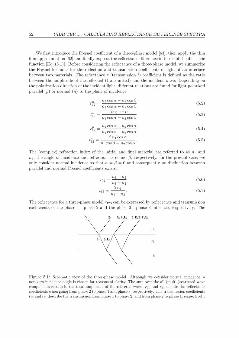
52 CHAPTER 5. CALCULATING REFLECTANCE DIFFERENCE SPECTRA
We first introduce the Fresnel coefficient of a three-phase model [63], then apply the thinfilm approximation [62] and finally express the reflectance difference in terms of the dielectricfunction [Eq. (5.1)]. Before considering the reflectance of a three-phase model, we summerizethe Fresnel formulas for the reflection and transmission coefficients of light at an interfacebetween two materials. The reflectance r (transmission t) coefficient is defined as the ratiobetween the amplitude of the reflected (transmitted) and the incident wave. Depending onthe polarization direction of the incident light, different relations are found for light polarizedparallel (p) or normal (n) to the plane of incidence:
rn12 =
n1 cosα− n2 cos β
n1 cosα+ n2 cos β(5.2)
tn12 =2n1 cosα
n1 cosα+ n2 cos β(5.3)
rp12 =
n1 cos β − n2 cosα
n1 cos β + n2 cosα(5.4)
tp12 =2n1 cosα
n1 cos β + n2 cosα. (5.5)
The (complex) refraction index of the initial and final material are referred to as n1 andn2, the angle of incidence and refraction as α and β, respectively. In the present case, weonly consider normal incidence so that α = β = 0 and consequently no distinction betweenparallel and normal Fresnel coefficients exists:
r12 =n1 − n2
n1 + n2(5.6)
t12 =2n1
n1 + n2. (5.7)
The reflectance for a three-phase model r123 can be expressed by reflectance and transmissioncoefficients of the phase 1 - phase 2 and the phase 2 - phase 3 interface, respectively. The
n2
n3
n1
r12
t12
t12t21
t12
r23 t12r23
r23
t21r23r21
Figure 5.1: Schematic view of the three-phase model. Although we consider normal incidence, anon-zero incidence angle is chosen for reasons of clarity. The sum over the all (multi-)scattered wavecomponents results in the total amplitude of the reflected wave. r21 and r23 denote the reflectancecoefficients when going from phase 2 to phase 1 and phase 3, respectively. The transmission coefficientst12 and t21 describe the transmission from phase 1 to phase 2, and from phase 2 to phase 1, respectively.
5.1. THREE-PHASE MODEL 53
procedure is schematically sketched in Fig. 5.1. If one considers (again assuming normalincidence), that the amplitude of a wave propagating inside a medium behaves as
A(z) = A0 e2πizn2/λ, (5.8)
the wave undergoes a change of e2iβ with β = 2 dπ n2/λ, when going from one side of thethin film and back again.2 The total amplitude of the reflected wave Ar therefore is givenby:
Ar = r12A0 + t21 r23 t12 e2iβA0 + t21 r23 r21 e
2iβr23 t12 e2iβA0 +
+ t21 r23 r21 e2iβr23 r21 e
2iβr23 t12 e2iβA0 + . . . . (5.9)
The reflectance coefficient of the three-phase model r123 = Ar/A0 consequently becomes:
r123 = r12 + t21 r23 t12 e2iβ(1 + r21 r23 e
2iβ + (r21 r23 e2iβ)2 + (r21 r23 e
2iβ)3 + . . .). (5.10)
By writing the sum of the geometrical series explicitely and replacing r21 by −r12, r123becomes:
r123 = r12 +t21 r23 t12 e
2iβ
1 + r12 r23 e2iβ. (5.11)
This expression can be transformed by applying Eq. (5.6) and Eq. (5.7)3:
r123 =r12 + r23 e
2iβ
1 + r12 r23 e2iβ. (5.12)
For d→ 0, the reflectance coefficient r13 has to be restored, so that
r13 =r12 + r23
1 + r12 r23. (5.13)
Until now, we have derived the reflectance of a three-phase model in terms of the reflectanceof two phases each. In order to obtain an explicit formula depending on the dielectric functionε = n2, we assume that the thickness of the film, d, is much smaller than the wavelength λof the incident light. As we will calculate the RD spectrum for light with energies rangingfrom 1 to 5 eV (corresponding to λ ≈ 1250 nm and ≈ 250 nm) and consider surface regionsof a few nm thickness, this assumption is reasonable. For the thin film case, the exponentialfunction can be expanded and by neglecting terms of order O(d2/λ2) one finds:
r123 =r12 + r23 (1 + 2iβ)
1 + r12 r23 (1 + 2iβ). (5.14)
Additionally, we consider the ratio between the reflectance of a three-phase model r123 andthe reflectance for d→ 0, r13:
r123r13
=1 + 2iβ [r23/(r12 + r23)]
1 + 2iβ [r12 r23/(1 + r12 r23)]. (5.15)
2If the space phase is chosen negative, as done in most optics text books, e2iβ is replaced by e−2iβ
3see also Heavens [63]. Again: different space phase.
54 CHAPTER 5. CALCULATING REFLECTANCE DIFFERENCE SPECTRA
Expansion of the denominator with respect to d/λ and again neglecting terms of higher orderin d/λ, the ratio becomes
r123r13
= 1 + 2 i β
[r23 (1− r212)
(r12 + r23)(1 + r12 r23)
]. (5.16)
Using the Fresnel formulas given in Eq. (5.6) and Eq. (5.7), we obtain:
r123r13
= 1 + 2 i β
(n1 n2
n22
)(n2
2 − n23
n21 − n
23
)= 1 + 2 i β
(n1 n2
n22
)(ε2 − ε3ε1 − ε3
). (5.17)
Replacing β by 2 dπ n2/λ the ratio becomes4
r123r13
= 1 +4πidn1
λ
(ε2 − ε3ε1 − ε3
). (5.18)
If we consider the first phase to be vacuum, than ε1 = 1 and n1 = 1. Additionally, weassume the bulk dielectric function (corresponding to ε3) to be isotropic and set ε3 = εb.The anisotropic dielectric tensor of the thin film ε2 will be referred to as εij . Instead of r123we write ri for the reflectance of light polarized in the (principle) direction i:
rir13
= 1 +4πid
λ
(εii − εb1− εb
)(5.19)
The reflectance difference is then given by:
2rx − ryrx + ry
= 2
[rxr13−ryr13
]/
[rxr13
+ryr13
]=
=
[4πid
λ
(εxx − εyy
1− εb
)]/
[1 +
2πid
λ
(εxx + εyy − 2εb
1− εb
)](5.20)
Applying again d/λ≪ 1, one finds:
∆r
r= −
4πid
λ
εxx − εyy
εb − 1(5.21)
proving Eq. (5.1).
Sometimes, the RD signal is not described via the reflectance r, but by considering thereflectivity R (see e.g., [64]), which describes the ratio between the squared amplitues of theincident and reflected waves. Applying the relation R = |r|2 and neglect terms of higherorder in d/λ the relative difference of reflectivities becomes:
∆R
R= −
8πd
λIm
[εxx − εyy
εb − 1
](5.22)
and consequently ∆R/R = −2Re[∆r/r].
4see also [62]. Different sign due to different space phase convention
5.2. CALCULATION OF THE DIELECTRIC FUNCTION 55
By writing real and imaginary parts explicitely, εb = ε(1)b +i ε
(2)b and ∆ε = ∆ε(1) +i∆ε(2),
the imaginary and real part of the RD signal are given by:
Re
[∆r
r
]=
4πd
λ
(∆ε(2) (ε
(1)b − 1)−∆ε(1) ε
(2)b
(ε(1)b − 1)2 + (ε
(2)b )2
)(5.23)
Im
[∆r
r
]= −
4πd
λ
(∆ε(2) ε
(2)b + ∆ε(1) (ε
(1)b − 1)
(ε(1)b − 1)2 + (ε
(2)b )2
). (5.24)
Thanks to the three-phase model, first-principles calculations of the reflectance anisotropyare possible, if one has access to the frequency dependent surface and bulk dielectric function.The surface dielectric anisotropy ∆ε of the thin film, the surface region, is thereby calculatedby modeling the surface as a slab consisting of several atomic layers. Following the derivationcarefully, it becomes clear that the only relevant quantity is d∆ε = d (εxx − εyy), which is asurface intrinsic property. As long as the depth, where the dielectric function is modified issmall compared to the wavelength, the derivation is accurate. Also note, that ε is proportionalto the polarizability per volume element [see Eq. (2.75)]. Thus d∆ε describes the differenceof the polarizability per surface area and is a well defined microscopic surface quantity.In the independent particle approximation (see below) one simply needs to normalize thepolarizability χKS to the surface area [1/A instead of 1/V ] to determine d∆ε.
5.2 Calculation of the dielectric function
By considering the three-phase model, we have obtained an expression for the reflectancedifference spectrum which depends on the dielectric function of the bulk and the (anisotropic)optical response of the surface. Because we are interested in the interaction of light and matterat optical wavelengths, the long-wavelength limit (q→ 0) is assumed in the following.
In an ab-initio calculation of the dielectric function several steps of increasing accuracy,but also complexity, can be considered. A detailed overview about different ways to calculatethe dielectric function and the relation between these methods can be found in [65]:
1. The dielectric function is calculated within the independent particle (IP) approximationon top of KS-DFT eigenenergies and wavefunctions. The dielectric tensor is then givenby Eq. (2.75).
2. Instead of the KS-DFT eigenenergies, quasiparticle energies calculated within Green’sfunction theory are used for the evaluation of the dielectric function. Normally, theG0W0 approximation is applied, and the quasiparticle energies are calculated as per-turbation to the KS-DFT energies. The dielectric function is again derived within theIP approximation, but the KS-DFT eigenenergies are now replaced by quasiparticleenergies.
3. Local field effects are included.
4. The inclusion of electron-hole interactions is realized by solving the Bethe-Salpeterequation. In the framework of Green’s function theory this can be described as theinclusion of vertex corrections in the description of the dielectric function.
56 CHAPTER 5. CALCULATING REFLECTANCE DIFFERENCE SPECTRA
Because calculations of surface optical properties are involved, most RD spectra of semicon-ductors and insulators (e.g., [66, 67, 68, 69, 70, 71]) and all theoretical RD spectra of metals[59, 60, 61, 72, 73, 74, 75] have been obtained applying the first and simplest approximation,so far. For exemplary semiconductor surfaces, as e.g., InP(001)-(2 × 4) and GaAs(110), alsocalculations employing the more involved independent quasiparticle approach exist [76, 67](step 2) resulting in an improved, but not perfect alignment with experiment. Local fieldeffects (step 3) and electron-hole interactions (step 4) have e.g., been included for the modelSi(110):H surface [77, 78, 79]. While the inclusion of local field effects has only a minorinfluence on the Si(110):H RD spectrum, the inclusion of electron-hole interactions via thesolution of the Bethe-Salpeter equation improves the correspondence with the experimentalspectrum. The Si(111)-(2×1) [80] and Ge(111)-(2×1) [81] surfaces are two further exampleswhere electron-hole interactions have been considered in the evaluation of the RD spectrum.
For the calculation of the bare and adsorbate covered Cu(110) RD spectra presentedin the following sections, we used the independent particle approximation applied on topof KS-DFT wavefunctions and eigenenergies (step 1). As a dense k-point grid and a largenumber of slab layers are required to obtain convergence of the RD signal, even at this levelof simplification, RD calculations for metallic surfaces are involved.
Nevertheless, two of the approximations applied for the calculation of the dielectric func-tion, namely the neglect of local field effects (step 3) and the electron-hole interaction (step4), are most likely more reliable for metals than for semiconductors. As calculations byMarini and co-workers [82] have shown, local field effects are negligible for the macroscopicdielectric function of bulk Cu. The reason for this can be found in the relatively homoge-nous screening in metals. The electron-hole interaction, on the other side, can be seen as anelectrostatic interaction between a negative (electron) and positive (hole) charged particlescreened by the dielectric function of the material. For metals the screening is large, so thatexcitonic effects should not be as important as for semiconductors and insulators.
Consequently, the approximation of the excitation energies by one-electron eigenenergiesobtained from KS-DFT remains the most important one. Not considering electron-holeinteractions, the use of KS-DFT eigenenergies will in particular result in a (not necessarilyuniform) shift of theoretical and experimental RD features whenever the calculated bandstructure does not match the measured photo emission (PE)/ inverse photo emission (IPE)spectrum.
Within the applied approximations, the imaginary part of the dielectric function ε(2) iscalculated via Eq. (2.73). The real part ε(1) is evaluated by a Kramers-Kronig transformation[Eq. (2.76)]. The wavefunctions and eigenenergies stem from KS-DFT calculations using theGGA-PBE approximation for the exchange-correlation potential. The theoretical lattice con-stant (3.638 A) was used for the bulk calculations. For the surfaces, symmetric slabs with upto 25 layers have been considered and the topmost 6 substrate layers and adsorbate positionshave been relaxed prior to the optical calculations. More details on the geometrical prop-erties of the bare Cu(110), the oxygen induced Cu(110)-(2 × 1)O added-row reconstruction,and the carbon monoxide covered Cu(110)-(2 × 1)CO and Cu(110)-(3 × 1)CO surfaces willbe given in Sec. 7.1. The intraband contributions to the dielectric functions are included bycalculating the intraband plasma tensor [Eq. (2.113)]. We found that an ab-initio treatmentof the anisotropic surface plasma frequency is essential in order to reduce the strong thicknessdependence due to band crossings near the Fermi-surface (see Sec. 2.9). The RD spectrum

5.2. CALCULATION OF THE DIELECTRIC FUNCTION 57
was finally evaluated by applying Eq. (5.1).For the interpretation of the resulting RD spectra in Sec. 7.3, we analyzed RD contri-
butions arising from specific k-point and energy regions. Important contributions to thetheoretical spectra could consequently be traced back to transitions between specific elec-tronic states. The agreement between experimental and theoretical RD spectra is not alwaysperfect, but the characteristic line-shapes could be qualitatively reproduced for all surfaces.
Chapter 6
Optical properties of bulk systems
6.1 Plasma frequencies
For metals, the long-wavelength dielectric function at small frequencies is dominated by in-traband transitions. In the independent particle approximation the real part of the dielectricfunction exhibits a −ω2/ω2 decay [Eq. (2.107)], where ω is the intraband plasma frequency[Eq. (2.113)]. This term is often referred to as Drude like term. In general, the plasma fre-quency is a tensor, but for the cubic metals considered in this chapter, it reduces to a scalarquantity. For the anisotropic surfaces treated in chapter 7, this is not the case anymore.
The intraband plasma frequency is calculated from a surface integral [see Eq. (2.113)].In order to generate a sufficient number of k-points in the vicinity of the Fermi surface,a very dense k-point mesh is required, so that the intraband plasma frequency convergessignificantly slower with the number of k-points than quantities which are evaluated from anintegral over the Brillouin zone volume (like energy and density). Faster convergence withthe number of k-points can be reached, if the smearing width σ for the determination of theone electron occupancies
f(ǫn) =1
1 + eǫn−µ
σ
(6.1)
is chosen larger (in practice often Gaussian broadening or, as in the present case, a Methfessel-Paxton broadening is chosen). In Tab 6.1, we report the copper plasma frequency (at theexperimental volume) for different sets of k-points and smearing widths. The k-point gridhas been generated using the Monkhorst-Pack scheme and for the broadening a Methfessel-Paxton method of first order with a smearing width σ has been applied.
For a relatively modest 16 × 16 × 16 k-point grid, a standard smearing width of 0.2 eVleads to an error of 0.5 eV in the intraband plasma frequency, whereas a 32 × 32 × 32 gridgives effectively converged plasma frequencies for all considered widths. For larger cells,where such dense k-point grids may not be practicable anymore, a large value of σ ≈ 0.4 eVseems to be a good compromise.
The same trend as is observed for copper has also been found for the other metals con-sidered in this chapter. The plasma frequencies ω obtained for a 32 k-point grid and σ = 0.2eV are summarized in Tab. 6.2. Additionally the number of electrons in partially filled bandsis given. If the band structure of a metal does not deviate too much from the free-electron
58
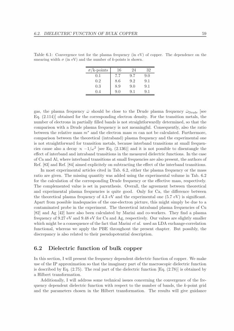
6.2. DIELECTRIC FUNCTION OF BULK COPPER 59
Table 6.1: Convergence test for the plasma frequency (in eV) of copper. The dependence on thesmearing width σ (in eV) and the number of k-points is shown.
σ/k-points 16 24 32
0.1 7.7 9.7 9.00.2 8.6 9.2 9.10.3 8.9 9.0 9.10.4 9.0 9.1 9.1
gas, the plasma frequency ω should be close to the Drude plasma frequency ωDrude [seeEq. (2.114)] obtained for the corresponding electron density. For the transition metals, thenumber of electrons in partially filled bands is not straightforwardly determined, so that thecomparison with a Drude plasma frequency is not meaningful. Consequently, also the ratiobetween the relative mass m∗ and the electron mass m can not be calculated. Furthermore,comparison between the theoretical (intraband) plasma frequency and the experimental oneis not straightforward for transition metals, because interband transitions at small frequen-cies cause also a decay ∝ −1/ω2 [see Eq. (2.136)] and it is not possible to disentangle theeffect of interband and intraband transitions in the measured dielectric functions. In the caseof Ca and Al, where interband transitions at small frequencies are also present, the authors ofRef. [83] and Ref. [84] aimed explicitely on subtracting the effect of the interband transitions.
In most experimental articles cited in Tab. 6.2, either the plasma frequency or the massratio are given. The missing quantity was added using the experimental volume in Tab. 6.2for the calculation of the corresponding Drude frequency or the effective mass, respectively.The complemented value is set in parenthesis. Overall, the agreement between theoreticaland experimental plasma frequencies is quite good. Only for Ca, the difference betweenthe theoretical plasma frequency of 4.3 eV and the experimental one (5.7 eV) is significant.Apart from possible inadequacies of the one-electron picture, this might simply be due to acontaminated probe in the experiment. The theoretical intraband plasma frequencies of Cu[82] and Ag [42] have also been calculated by Marini and co-workers. They find a plasmafrequency of 9.27 eV and 9.48 eV for Cu and Ag, respectively. Our values are slightly smallerwhich might be a consequence of the fact that Marini et al. used an LDA exchange-correlationfunctional, whereas we apply the PBE throughout the present chapter. But possibly, thediscrepancy is also related to their pseudopotential description.
6.2 Dielectric function of bulk copper
In this section, I will present the frequency dependent dielectric function of copper. We makeuse of the IP approximation so that the imaginary part of the macroscopic dielectric functionis described by Eq. (2.75). The real part of the dielectric function [Eq. (2.78)] is obtained bya Hilbert transformation.
Additionally, I will address some technical issues concerning the convergence of the fre-quency dependent dielectric function with respect to the number of bands, the k-point gridand the parameters chosen in the Hilbert transformation. The results will give guidance
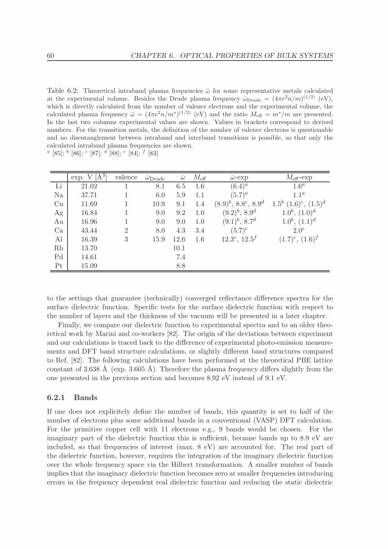
60 CHAPTER 6. OPTICAL PROPERTIES OF BULK SYSTEMS
Table 6.2: Theoretical intraband plasma frequencies ω for some representative metals calculatedat the experimental volume. Besides the Drude plasma frequency ωDrude = (4πe2n/m)(1/2) (eV),which is directly calculated from the number of valence electrons and the experimental volume, thecalculated plasma frequency ω = (4πe2n/m∗)(1/2) (eV) and the ratio Meff = m∗/m are presented.In the last two columns experimental values are shown. Values in brackets correspond to derivednumbers. For the transition metals, the definition of the number of valence electrons is questionableand no disentanglement between intraband and interband transitions is possible, so that only thecalculated intraband plasma frequencies are shown.a [85]; b [86]; c [87]; d [88]; e [84]; f [83]
exp. V [A3] valence ωDrude ω Meff ω-exp Meff -exp
Li 21.02 1 8.1 6.5 1.6 (6.4)a 1.6a
Na 37.71 1 6.0 5.9 1.1 (5.7)a 1.1a
Cu 11.69 1 10.9 9.1 1.4 (8.9)b, 8.8c, 8.9d 1.5b (1.6)c, (1.5)d
Ag 16.84 1 9.0 9.2 1.0 (9.2)b, 8.9d 1.0b, (1.0)d
Au 16.96 1 9.0 9.0 1.0 (9.1)b, 8.7d 1.0b, (1.1)d
Ca 43.44 2 8.0 4.3 3.4 (5.7)e 2.0e
Al 16.39 3 15.9 12.6 1.6 12.3c, 12.5f (1.7)c, (1.6)f
Rh 13.70 10.1Pd 14.61 7.4Pt 15.09 8.8
to the settings that guarantee (technically) converged reflectance difference spectra for thesurface dielectric function. Specific tests for the surface dielectric function with respect tothe number of layers and the thickness of the vacuum will be presented in a later chapter.
Finally, we compare our dielectric function to experimental spectra and to an older theo-retical work by Marini and co-workers [82]. The origin of the deviations between experimentand our calculations is traced back to the difference of experimental photo-emission measure-ments and DFT band structure calculations, or slightly different band structures comparedto Ref. [82]. The following calculations have been performed at the theoretical PBE latticeconstant of 3.638 A (exp. 3.605 A). Therefore the plasma frequency differs slightly from theone presented in the previous section and becomes 8.92 eV instead of 9.1 eV.
6.2.1 Bands
If one does not explicitely define the number of bands, this quantity is set to half of thenumber of electrons plus some additional bands in a conventional (VASP) DFT calculation.For the primitive copper cell with 11 electrons e.g., 9 bands would be chosen. For theimaginary part of the dielectric function this is sufficient, because bands up to 8.9 eV areincluded, so that frequencies of interest (max. 8 eV) are accounted for. The real part ofthe dielectric function, however, requires the integration of the imaginary dielectric functionover the whole frequency space via the Hilbert transformation. A smaller number of bandsimplies that the imaginary dielectric function becomes zero at smaller frequencies introducingerrors in the frequency dependent real dielectric function and reducing the static dielectric
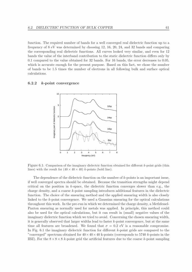
6.2. DIELECTRIC FUNCTION OF BULK COPPER 61
function. The required number of bands for a well converged real dielectric function up to afrequency of 8 eV was determined by choosing 12, 16, 20, 24, and 32 bands and comparingthe corresponding real dielectric functions. All curves looked very similar, and even for 12bands the value of the interband contribution to the static dielectric function differs only by0.1 compared to the value obtained for 32 bands. For 16 bands, the error decreases to 0.05,which is accurate enough for the present purpose. Based on this fact, we chose the numberof bands to be 1.5 times the number of electrons in all following bulk and surface opticalcalculations.
6.2.2 k-point convergence
10
5
0
0 1 2 3 4 5 6 7 8
imag
inar
y pa
rt o
f die
lect
ric fu
nctio
n
freuqency (eV)
8kp
16kp
24kp
32kp
Figure 6.1: Comparison of the imaginary dielectric function obtained for different k-point grids (thinlines) with the result for (40× 40× 40) k-points (bold line).
The dependence of the dielectric function on the number of k-points is an important issue,if well converged spectra should be obtained. Because the transition strengths might dependcritical on the position in k-space, the dielectric function converges slower than e.g., thecharge density, and a coarse k-point sampling introduces additional features in the dielectricfunction. The choice of the smearing method and the applied smearing width is also closelylinked to the k-point convergence. We used a Gaussian smearing for the optical calculationsthroughout this work. In the pre-run in which we determined the charge density, a Methfessel-Paxton smearing as normally used for metals was applied. In principle, this method couldalso be used for the optical calculations, but it can result in (small) negative values of theimaginary dielectric function which we tried to avoid. Concerning the chosen smearing width,it is generally observed that larger widths lead to faster k-point convergence, but at the sametime all features are broadened. We found that σ = 0.2 eV is a reasonable compromise.In Fig. 6.1 the imaginary dielectric function for different k-point grids are compared to the”converged” spectrum obtained for 40×40×40 k-points (corresponds to 5740 k-points in theIBZ). For the 8× 8× 8 k-point grid the artificial features due to the coarse k-point sampling
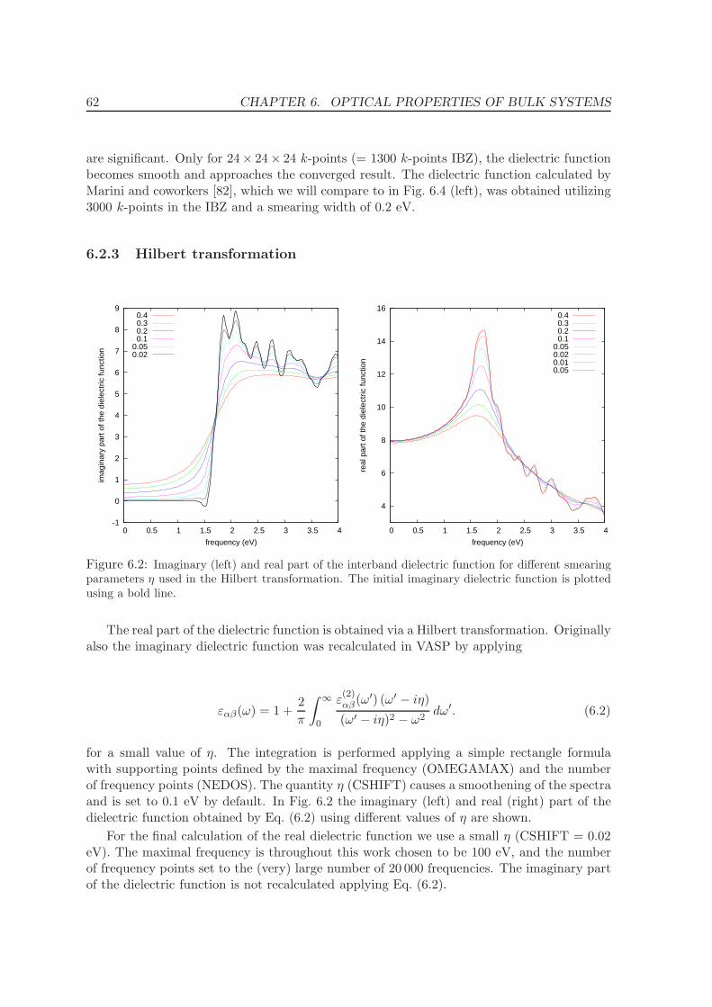
62 CHAPTER 6. OPTICAL PROPERTIES OF BULK SYSTEMS
are significant. Only for 24× 24× 24 k-points (= 1300 k-points IBZ), the dielectric functionbecomes smooth and approaches the converged result. The dielectric function calculated byMarini and coworkers [82], which we will compare to in Fig. 6.4 (left), was obtained utilizing3000 k-points in the IBZ and a smearing width of 0.2 eV.
6.2.3 Hilbert transformation
-1
0
1
2
3
4
5
6
7
8
9
0 0.5 1 1.5 2 2.5 3 3.5 4
imag
inar
y pa
rt o
f the
die
lect
ric fu
nctio
n
frequency (eV)
0.40.30.20.1
0.050.02
4
6
8
10
12
14
16
0 0.5 1 1.5 2 2.5 3 3.5 4
real
par
t of t
he d
iele
ctric
func
tion
frequency (eV)
0.40.30.20.1
0.050.020.010.05
Figure 6.2: Imaginary (left) and real part of the interband dielectric function for different smearingparameters η used in the Hilbert transformation. The initial imaginary dielectric function is plottedusing a bold line.
The real part of the dielectric function is obtained via a Hilbert transformation. Originallyalso the imaginary dielectric function was recalculated in VASP by applying
εαβ(ω) = 1 +2
π
∫ ∞
0
ε(2)αβ(ω′) (ω′ − iη)
(ω′ − iη)2 − ω2dω′. (6.2)
for a small value of η. The integration is performed applying a simple rectangle formulawith supporting points defined by the maximal frequency (OMEGAMAX) and the numberof frequency points (NEDOS). The quantity η (CSHIFT) causes a smoothening of the spectraand is set to 0.1 eV by default. In Fig. 6.2 the imaginary (left) and real (right) part of thedielectric function obtained by Eq. (6.2) using different values of η are shown.
For the final calculation of the real dielectric function we use a small η (CSHIFT = 0.02eV). The maximal frequency is throughout this work chosen to be 100 eV, and the numberof frequency points set to the (very) large number of 20 000 frequencies. The imaginary partof the dielectric function is not recalculated applying Eq. (6.2).
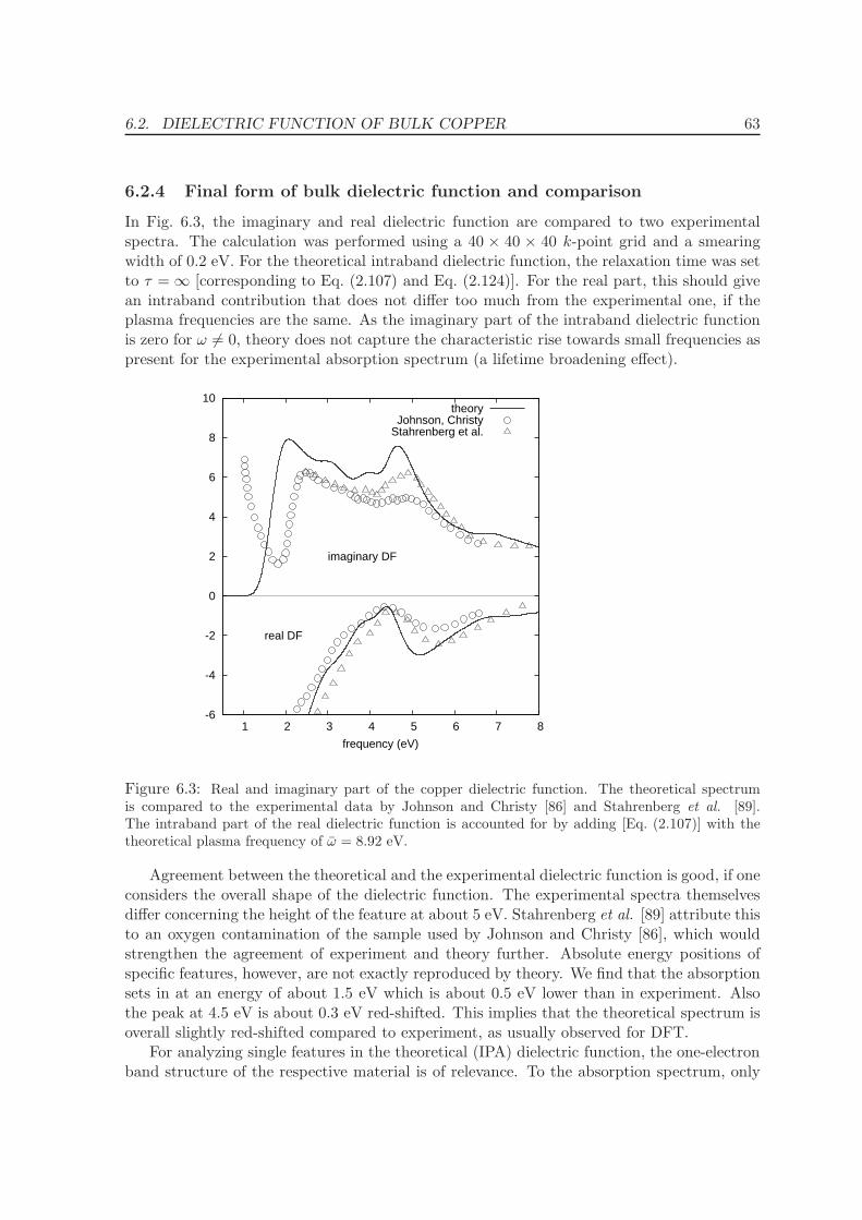
6.2. DIELECTRIC FUNCTION OF BULK COPPER 63
6.2.4 Final form of bulk dielectric function and comparison
In Fig. 6.3, the imaginary and real dielectric function are compared to two experimentalspectra. The calculation was performed using a 40 × 40 × 40 k-point grid and a smearingwidth of 0.2 eV. For the theoretical intraband dielectric function, the relaxation time was setto τ =∞ [corresponding to Eq. (2.107) and Eq. (2.124)]. For the real part, this should givean intraband contribution that does not differ too much from the experimental one, if theplasma frequencies are the same. As the imaginary part of the intraband dielectric functionis zero for ω 6= 0, theory does not capture the characteristic rise towards small frequencies aspresent for the experimental absorption spectrum (a lifetime broadening effect).
-6
-4
-2
0
2
4
6
8
10
1 2 3 4 5 6 7 8
frequency (eV)
imaginary DF
real DF
theoryJohnson, Christy
Stahrenberg et al.
Figure 6.3: Real and imaginary part of the copper dielectric function. The theoretical spectrumis compared to the experimental data by Johnson and Christy [86] and Stahrenberg et al. [89].The intraband part of the real dielectric function is accounted for by adding [Eq. (2.107)] with thetheoretical plasma frequency of ω = 8.92 eV.
Agreement between the theoretical and the experimental dielectric function is good, if oneconsiders the overall shape of the dielectric function. The experimental spectra themselvesdiffer concerning the height of the feature at about 5 eV. Stahrenberg et al. [89] attribute thisto an oxygen contamination of the sample used by Johnson and Christy [86], which wouldstrengthen the agreement of experiment and theory further. Absolute energy positions ofspecific features, however, are not exactly reproduced by theory. We find that the absorptionsets in at an energy of about 1.5 eV which is about 0.5 eV lower than in experiment. Alsothe peak at 4.5 eV is about 0.3 eV red-shifted. This implies that the theoretical spectrum isoverall slightly red-shifted compared to experiment, as usually observed for DFT.
For analyzing single features in the theoretical (IPA) dielectric function, the one-electronband structure of the respective material is of relevance. To the absorption spectrum, only
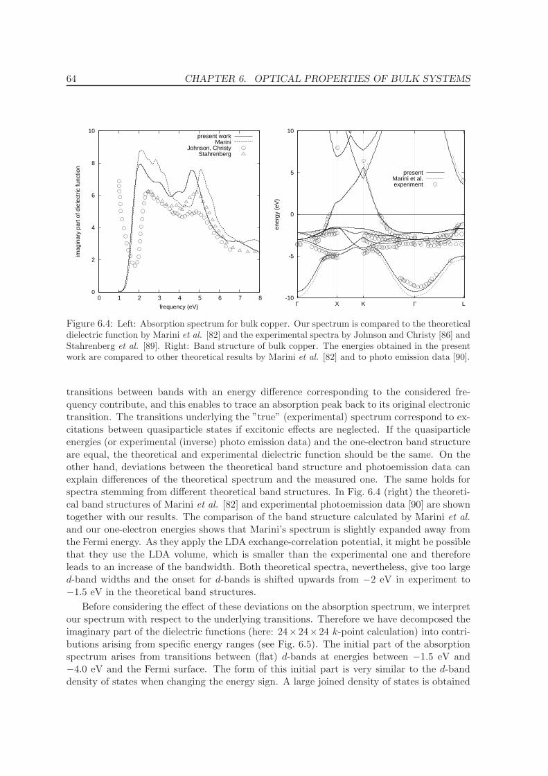
64 CHAPTER 6. OPTICAL PROPERTIES OF BULK SYSTEMS
0
2
4
6
8
10
0 1 2 3 4 5 6 7 8
imag
inar
y pa
rt o
f die
lect
ric fu
nctio
n
frequency (eV)
present workMarini
Johnson, ChristyStahrenberg
-10
-5
0
5
10
LΓKXΓ
ener
gy (
eV)
presentMarini et al.experiment
Figure 6.4: Left: Absorption spectrum for bulk copper. Our spectrum is compared to the theoreticaldielectric function by Marini et al. [82] and the experimental spectra by Johnson and Christy [86] andStahrenberg et al. [89]. Right: Band structure of bulk copper. The energies obtained in the presentwork are compared to other theoretical results by Marini et al. [82] and to photo emission data [90].
transitions between bands with an energy difference corresponding to the considered fre-quency contribute, and this enables to trace an absorption peak back to its original electronictransition. The transitions underlying the ”true” (experimental) spectrum correspond to ex-citations between quasiparticle states if excitonic effects are neglected. If the quasiparticleenergies (or experimental (inverse) photo emission data) and the one-electron band structureare equal, the theoretical and experimental dielectric function should be the same. On theother hand, deviations between the theoretical band structure and photoemission data canexplain differences of the theoretical spectrum and the measured one. The same holds forspectra stemming from different theoretical band structures. In Fig. 6.4 (right) the theoreti-cal band structures of Marini et al. [82] and experimental photoemission data [90] are showntogether with our results. The comparison of the band structure calculated by Marini et al.and our one-electron energies shows that Marini’s spectrum is slightly expanded away fromthe Fermi energy. As they apply the LDA exchange-correlation potential, it might be possiblethat they use the LDA volume, which is smaller than the experimental one and thereforeleads to an increase of the bandwidth. Both theoretical spectra, nevertheless, give too larged-band widths and the onset for d-bands is shifted upwards from −2 eV in experiment to−1.5 eV in the theoretical band structures.
Before considering the effect of these deviations on the absorption spectrum, we interpretour spectrum with respect to the underlying transitions. Therefore we have decomposed theimaginary part of the dielectric functions (here: 24×24×24 k-point calculation) into contri-butions arising from specific energy ranges (see Fig. 6.5). The initial part of the absorptionspectrum arises from transitions between (flat) d-bands at energies between −1.5 eV and−4.0 eV and the Fermi surface. The form of this initial part is very similar to the d-banddensity of states when changing the energy sign. A large joined density of states is obtained
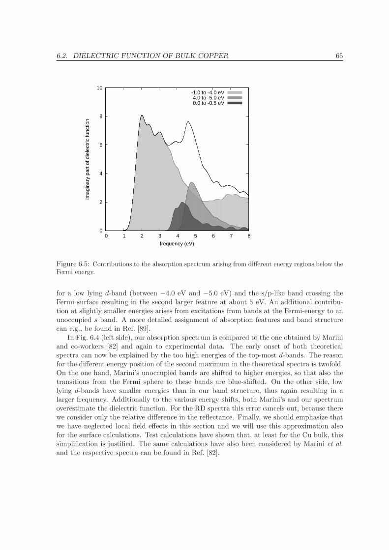
6.2. DIELECTRIC FUNCTION OF BULK COPPER 65
0
2
4
6
8
10
0 1 2 3 4 5 6 7 8
imag
inar
y pa
rt o
f die
lect
ric fu
nctio
n
frequency (eV)
-1.0 to -4.0 eV-4.0 to -5.0 eV 0.0 to -0.5 eV
Figure 6.5: Contributions to the absorption spectrum arising from different energy regions below theFermi energy.
for a low lying d-band (between −4.0 eV and −5.0 eV) and the s/p-like band crossing theFermi surface resulting in the second larger feature at about 5 eV. An additional contribu-tion at slightly smaller energies arises from excitations from bands at the Fermi-energy to anunoccupied s band. A more detailed assignment of absorption features and band structurecan e.g., be found in Ref. [89].
In Fig. 6.4 (left side), our absorption spectrum is compared to the one obtained by Mariniand co-workers [82] and again to experimental data. The early onset of both theoreticalspectra can now be explained by the too high energies of the top-most d-bands. The reasonfor the different energy position of the second maximum in the theoretical spectra is twofold.On the one hand, Marini’s unoccupied bands are shifted to higher energies, so that also thetransitions from the Fermi sphere to these bands are blue-shifted. On the other side, lowlying d-bands have smaller energies than in our band structure, thus again resulting in alarger frequency. Additionally to the various energy shifts, both Marini’s and our spectrumoverestimate the dielectric function. For the RD spectra this error cancels out, because therewe consider only the relative difference in the reflectance. Finally, we should emphasize thatwe have neglected local field effects in this section and we will use this approximation alsofor the surface calculations. Test calculations have shown that, at least for the Cu bulk, thissimplification is justified. The same calculations have also been considered by Marini et al.and the respective spectra can be found in Ref. [82].
Chapter 7
Optical calculations for Cu(110)surfaces
In this chapter, we will present reflectance difference spectra for the bare, the oxygen, andthe carbon monoxide covered Cu(110) surface. The Cu(110) surface has been one of the firstmetallic surfaces studied with RD spectroscopy [52] and has evoked numerous experimentalstudies since [53, 54, 55, 56, 57, 58]. Additionally the electronic structure of the bare andoxygen covered Cu(110) surface is well studied by (inverse) photoemission spectroscopy [92,93, 94, 95], thus allowing an easy check of the validity of the theoretical one-electron bandstructure. This makes the bare Cu(110) and its adsorbate covered surfaces a good test casefor surface optical calculations. RD spectra have already been evaluated for the bare [59, 60]and carbon-monoxide covered [61] Cu(110) surface by Monachesi and coworkers. Their linearmuffin tin orbital (LMTO) calculations were based on the independent particle approximationfor the (surface) dielectric function, as is the case in the present work. The RD spectra ofMonachesi et al. shared some features with the experimental spectra, but due to their smallnumber of slab layers (11 layers) the overall agreement with experiment was modest.
In the following section, we first give a brief overview of the geometry of the bare Cu(110),the Cu(110)-(2×1)O, the Cu(110)-(2×1)CO, and the Cu(110)-(3×1)CO surface. Afterwards,convergence tests for the surface optical response with respect to the number of k-points, thevacuum layer thickness, and the number of slab layers will be presented. Finally, the RDspectra of the considered surface structure are shown in Sec. 7.3 and interpreted with respectto the theoretical band structure presented in Sec. 7.3.1.
7.1 Geometry of surfaces
In this section, a brief overview of the considered surface structures will be given. Fig. 7.1shows the bare Cu(110) surface in top view. Here and in the following sections the [110],[001], and [110] direction will be referred to as x-, y-, and z-direction, respectively. Theanisotropy of the bare (110) surface arises from the different distance of surface atoms in x-and y- direction (2.572 A along the x-direction, 3.638 A along the y-direction). For the bareCu(110) surface the distance of the two topmost layers d12 is 1.16 A, which is −10 % smallerthan the bulk layer distance of 1.286 A. For the second and third layer, the layer distanced23 is increased by 4.5 %.
66
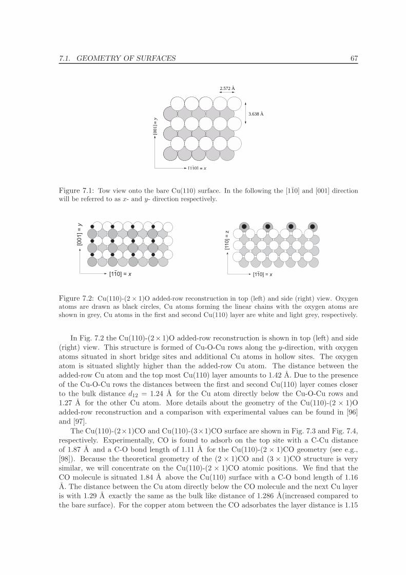
7.1. GEOMETRY OF SURFACES 67
3.638 A
2.572 A
[110]
[001
]
= x
= y
Figure 7.1: Tow view onto the bare Cu(110) surface. In the following the [110] and [001] directionwill be referred to as x- and y- direction respectively.
[110] = x
[001] =
y
[110] = x
[11
0]
= z
Figure 7.2: Cu(110)-(2× 1)O added-row reconstruction in top (left) and side (right) view. Oxygenatoms are drawn as black circles, Cu atoms forming the linear chains with the oxygen atoms areshown in grey, Cu atoms in the first and second Cu(110) layer are white and light grey, respectively.
In Fig. 7.2 the Cu(110)-(2× 1)O added-row reconstruction is shown in top (left) and side(right) view. This structure is formed of Cu-O-Cu rows along the y-direction, with oxygenatoms situated in short bridge sites and additional Cu atoms in hollow sites. The oxygenatom is situated slightly higher than the added-row Cu atom. The distance between theadded-row Cu atom and the top most Cu(110) layer amounts to 1.42 A. Due to the presenceof the Cu-O-Cu rows the distances between the first and second Cu(110) layer comes closerto the bulk distance d12 = 1.24 A for the Cu atom directly below the Cu-O-Cu rows and1.27 A for the other Cu atom. More details about the geometry of the Cu(110)-(2 × 1)Oadded-row reconstruction and a comparison with experimental values can be found in [96]and [97].
The Cu(110)-(2×1)CO and Cu(110)-(3×1)CO surface are shown in Fig. 7.3 and Fig. 7.4,respectively. Experimentally, CO is found to adsorb on the top site with a C-Cu distanceof 1.87 A and a C-O bond length of 1.11 A for the Cu(110)-(2 × 1)CO geometry (see e.g.,[98]). Because the theoretical geometry of the (2 × 1)CO and (3 × 1)CO structure is verysimilar, we will concentrate on the Cu(110)-(2 × 1)CO atomic positions. We find that theCO molecule is situated 1.84 A above the Cu(110) surface with a C-O bond length of 1.16A. The distance between the Cu atom directly below the CO molecule and the next Cu layeris with 1.29 A exactly the same as the bulk like distance of 1.286 A(increased compared tothe bare surface). For the copper atom between the CO adsorbates the layer distance is 1.15
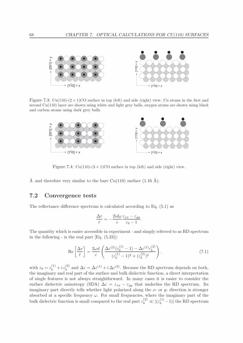
68 CHAPTER 7. OPTICAL CALCULATIONS FOR CU(110) SURFACES
[110] = x
[001] =
y
[110] = x
[11
0]
=z
Figure 7.3: Cu(110)-(2× 1)CO surface in top (left) and side (right) view. Cu atoms in the first andsecond Cu(110) layer are shown using white and light grey balls, oxygen atoms are shown using blackand carbon atoms using dark grey balls.
[110] = x
[001] =
y
[110] = x
[11
0]
=z
Figure 7.4: Cu(110)-(3× 1)CO surface in top (left) and side (right) view.
A and therefore very similar to the bare Cu(110) surface (1.16 A).
7.2 Convergence tests
The reflectance difference spectrum is calculated according to Eq. (5.1) as
∆r
r= −
2idω
c
εxx − εyy
εb − 1.
The quantity which is easier accessible in experiment - and simply referred to as RD spectrumin the following - is the real part [Eq. (5.23)]:
Re
[∆r
r
]=
2ωd
c
(∆ε(2)(ε
(1)b − 1)−∆ε(1)ε
(2)b
(ε(1)b − 1)2 + (ε
(2)b )2
). (7.1)
with εb = ε(1)b + i ε
(2)b and ∆ε = ∆ε(1) + i∆ε(2). Because the RD spectrum depends on both,
the imaginary and real part of the surface and bulk dielectric function, a direct interpretationof single features is not always straightforward. In many cases it is easier to consider thesurface dielectric anisotropy (SDA) ∆ε = εxx − εyy that underlies the RD spectrum. Itsimaginary part directly tells whether light polarized along the x- or y- direction is strongerabsorbed at a specific frequency ω. For small frequencies, where the imaginary part of the
bulk dielectric function is small compared to the real part ε(2)b ≪ |(ε
(1)b −1)| the RD spectrum
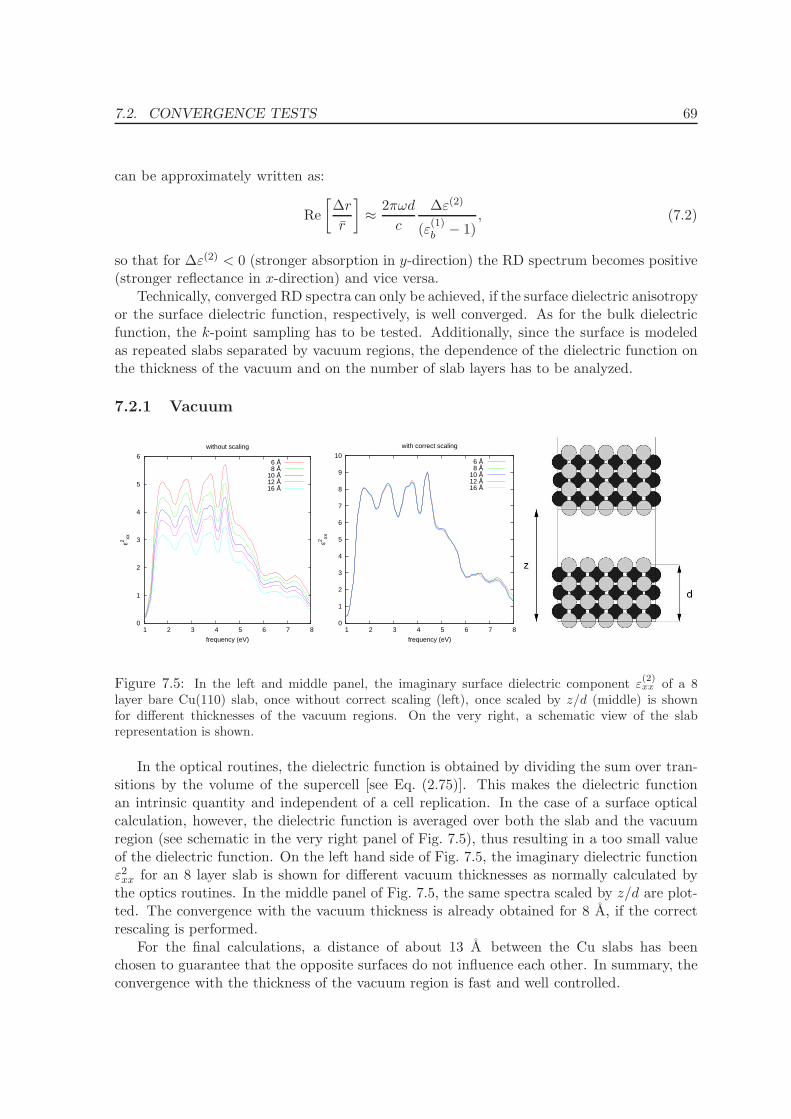
7.2. CONVERGENCE TESTS 69
can be approximately written as:
Re
[∆r
r
]≈
2πωd
c
∆ε(2)
(ε(1)b − 1)
, (7.2)
so that for ∆ε(2) < 0 (stronger absorption in y-direction) the RD spectrum becomes positive(stronger reflectance in x-direction) and vice versa.
Technically, converged RD spectra can only be achieved, if the surface dielectric anisotropyor the surface dielectric function, respectively, is well converged. As for the bulk dielectricfunction, the k-point sampling has to be tested. Additionally, since the surface is modeledas repeated slabs separated by vacuum regions, the dependence of the dielectric function onthe thickness of the vacuum and on the number of slab layers has to be analyzed.
7.2.1 Vacuum
0
1
2
3
4
5
6
1 2 3 4 5 6 7 8
ε2 xx
frequency (eV)
without scaling
6 Å8 Å
10 Å12 Å16 Å
0
1
2
3
4
5
6
7
8
9
10
1 2 3 4 5 6 7 8
ε2 xx
frequency (eV)
with correct scaling
6 Å8 Å
10 Å12 Å16 Å
Figure 7.5: In the left and middle panel, the imaginary surface dielectric component ε(2)xx of a 8
layer bare Cu(110) slab, once without correct scaling (left), once scaled by z/d (middle) is shownfor different thicknesses of the vacuum regions. On the very right, a schematic view of the slabrepresentation is shown.
In the optical routines, the dielectric function is obtained by dividing the sum over tran-sitions by the volume of the supercell [see Eq. (2.75)]. This makes the dielectric functionan intrinsic quantity and independent of a cell replication. In the case of a surface opticalcalculation, however, the dielectric function is averaged over both the slab and the vacuumregion (see schematic in the very right panel of Fig. 7.5), thus resulting in a too small valueof the dielectric function. On the left hand side of Fig. 7.5, the imaginary dielectric functionε2xx for an 8 layer slab is shown for different vacuum thicknesses as normally calculated bythe optics routines. In the middle panel of Fig. 7.5, the same spectra scaled by z/d are plot-ted. The convergence with the vacuum thickness is already obtained for 8 A, if the correctrescaling is performed.
For the final calculations, a distance of about 13 A between the Cu slabs has beenchosen to guarantee that the opposite surfaces do not influence each other. In summary, theconvergence with the thickness of the vacuum region is fast and well controlled.
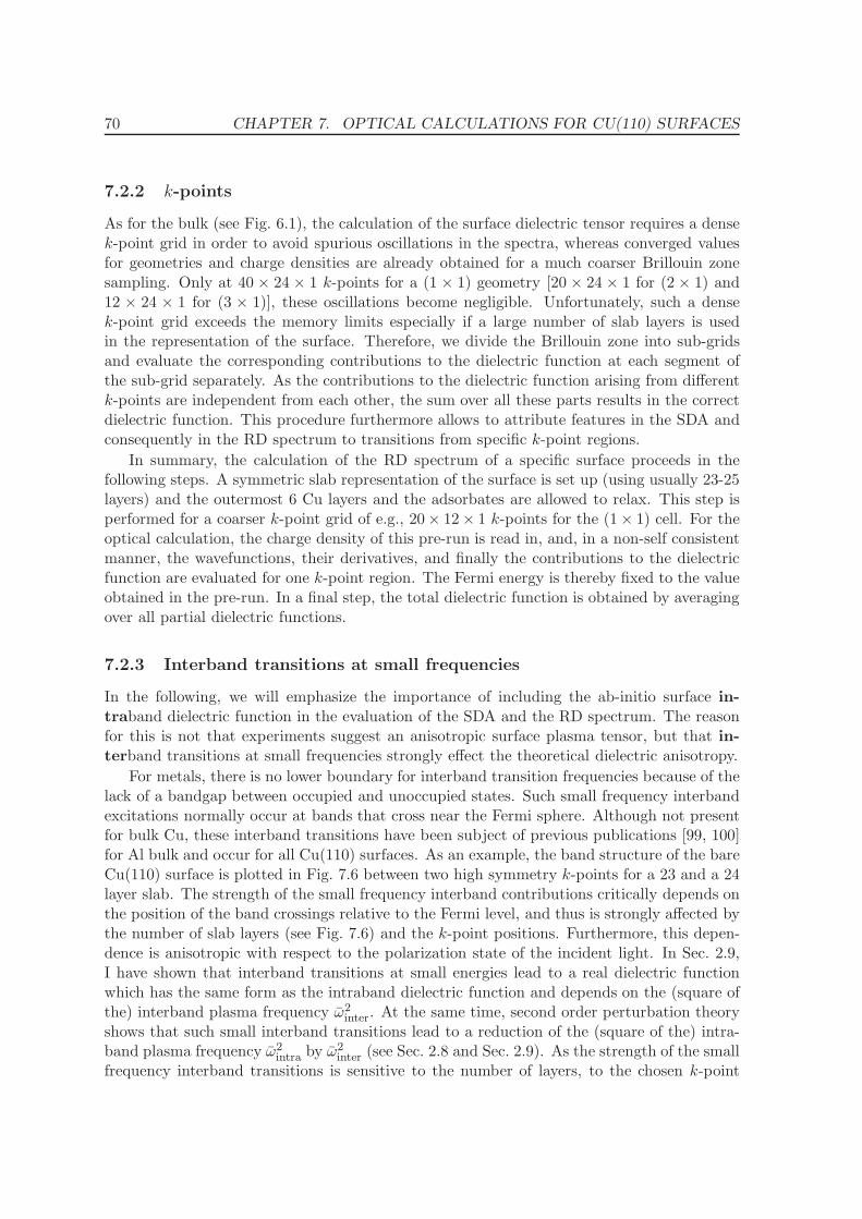
70 CHAPTER 7. OPTICAL CALCULATIONS FOR CU(110) SURFACES
7.2.2 k-points
As for the bulk (see Fig. 6.1), the calculation of the surface dielectric tensor requires a densek-point grid in order to avoid spurious oscillations in the spectra, whereas converged valuesfor geometries and charge densities are already obtained for a much coarser Brillouin zonesampling. Only at 40 × 24 × 1 k-points for a (1 × 1) geometry [20 × 24 × 1 for (2 × 1) and12 × 24 × 1 for (3 × 1)], these oscillations become negligible. Unfortunately, such a densek-point grid exceeds the memory limits especially if a large number of slab layers is usedin the representation of the surface. Therefore, we divide the Brillouin zone into sub-gridsand evaluate the corresponding contributions to the dielectric function at each segment ofthe sub-grid separately. As the contributions to the dielectric function arising from differentk-points are independent from each other, the sum over all these parts results in the correctdielectric function. This procedure furthermore allows to attribute features in the SDA andconsequently in the RD spectrum to transitions from specific k-point regions.
In summary, the calculation of the RD spectrum of a specific surface proceeds in thefollowing steps. A symmetric slab representation of the surface is set up (using usually 23-25layers) and the outermost 6 Cu layers and the adsorbates are allowed to relax. This step isperformed for a coarser k-point grid of e.g., 20× 12× 1 k-points for the (1× 1) cell. For theoptical calculation, the charge density of this pre-run is read in, and, in a non-self consistentmanner, the wavefunctions, their derivatives, and finally the contributions to the dielectricfunction are evaluated for one k-point region. The Fermi energy is thereby fixed to the valueobtained in the pre-run. In a final step, the total dielectric function is obtained by averagingover all partial dielectric functions.
7.2.3 Interband transitions at small frequencies
In the following, we will emphasize the importance of including the ab-initio surface in-traband dielectric function in the evaluation of the SDA and the RD spectrum. The reasonfor this is not that experiments suggest an anisotropic surface plasma tensor, but that in-terband transitions at small frequencies strongly effect the theoretical dielectric anisotropy.
For metals, there is no lower boundary for interband transition frequencies because of thelack of a bandgap between occupied and unoccupied states. Such small frequency interbandexcitations normally occur at bands that cross near the Fermi sphere. Although not presentfor bulk Cu, these interband transitions have been subject of previous publications [99, 100]for Al bulk and occur for all Cu(110) surfaces. As an example, the band structure of the bareCu(110) surface is plotted in Fig. 7.6 between two high symmetry k-points for a 23 and a 24layer slab. The strength of the small frequency interband contributions critically depends onthe position of the band crossings relative to the Fermi level, and thus is strongly affected bythe number of slab layers (see Fig. 7.6) and the k-point positions. Furthermore, this depen-dence is anisotropic with respect to the polarization state of the incident light. In Sec. 2.9,I have shown that interband transitions at small energies lead to a real dielectric functionwhich has the same form as the intraband dielectric function and depends on the (square ofthe) interband plasma frequency ω2
inter. At the same time, second order perturbation theoryshows that such small interband transitions lead to a reduction of the (square of the) intra-band plasma frequency ω2
intra by ω2inter (see Sec. 2.8 and Sec. 2.9). As the strength of the small
frequency interband transitions is sensitive to the number of layers, to the chosen k-point
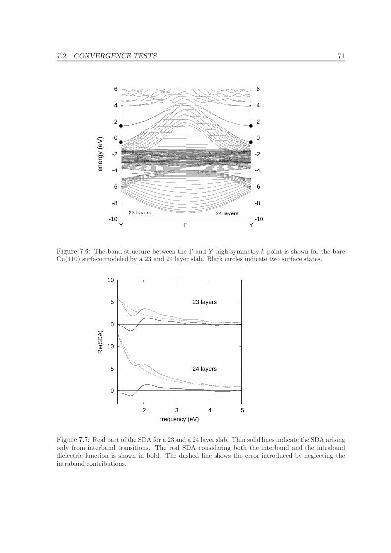
7.2. CONVERGENCE TESTS 71
-10
-8
-6
-4
-2
0
2
4
6
Y Γ Y-10
-8
-6
-4
-2
0
2
4
6
ener
gy (
eV)
24 layers23 layers
Figure 7.6: The band structure between the Γ and Y high symmetry k-point is shown for the bareCu(110) surface modeled by a 23 and 24 layer slab. Black circles indicate two surface states.
0
5
10
0
5
10
2 3 4 5
Re(
SD
A)
frequency (eV)
24 layers
23 layers
Figure 7.7: Real part of the SDA for a 23 and a 24 layer slab. Thin solid lines indicate the SDA arisingonly from interband transitions. The real SDA considering both the interband and the intrabanddielectric function is shown in bold. The dashed line shows the error introduced by neglecting theintraband contributions.
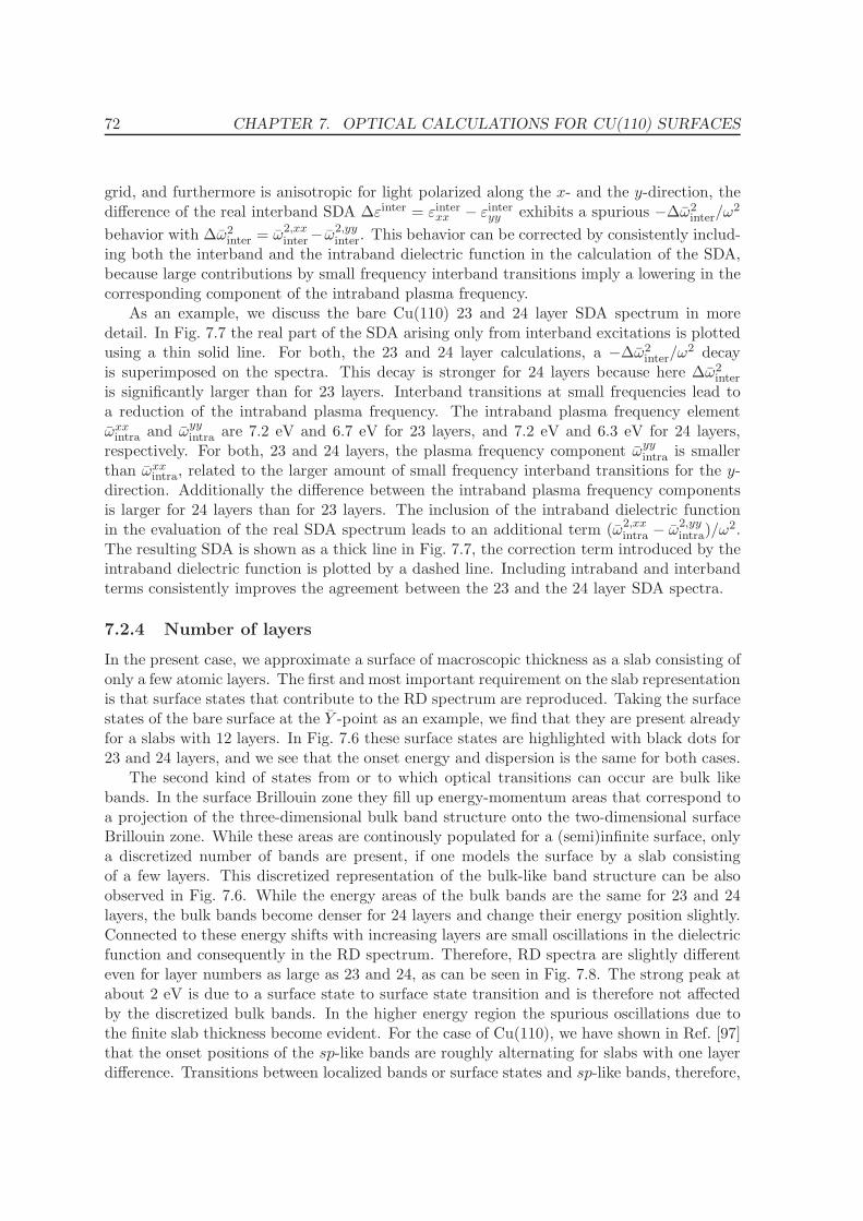
72 CHAPTER 7. OPTICAL CALCULATIONS FOR CU(110) SURFACES
grid, and furthermore is anisotropic for light polarized along the x- and the y-direction, thedifference of the real interband SDA ∆εinter = εinter
xx − εinteryy exhibits a spurious −∆ω2
inter/ω2
behavior with ∆ω2inter = ω2,xx
inter− ω2,yyinter. This behavior can be corrected by consistently includ-
ing both the interband and the intraband dielectric function in the calculation of the SDA,because large contributions by small frequency interband transitions imply a lowering in thecorresponding component of the intraband plasma frequency.
As an example, we discuss the bare Cu(110) 23 and 24 layer SDA spectrum in moredetail. In Fig. 7.7 the real part of the SDA arising only from interband excitations is plottedusing a thin solid line. For both, the 23 and 24 layer calculations, a −∆ω2
inter/ω2 decay
is superimposed on the spectra. This decay is stronger for 24 layers because here ∆ω2inter
is significantly larger than for 23 layers. Interband transitions at small frequencies lead toa reduction of the intraband plasma frequency. The intraband plasma frequency elementωxx
intra and ωyyintra are 7.2 eV and 6.7 eV for 23 layers, and 7.2 eV and 6.3 eV for 24 layers,
respectively. For both, 23 and 24 layers, the plasma frequency component ωyyintra is smaller
than ωxxintra, related to the larger amount of small frequency interband transitions for the y-
direction. Additionally the difference between the intraband plasma frequency componentsis larger for 24 layers than for 23 layers. The inclusion of the intraband dielectric functionin the evaluation of the real SDA spectrum leads to an additional term (ω2,xx
intra − ω2,yyintra)/ω
2.The resulting SDA is shown as a thick line in Fig. 7.7, the correction term introduced by theintraband dielectric function is plotted by a dashed line. Including intraband and interbandterms consistently improves the agreement between the 23 and the 24 layer SDA spectra.
7.2.4 Number of layers
In the present case, we approximate a surface of macroscopic thickness as a slab consisting ofonly a few atomic layers. The first and most important requirement on the slab representationis that surface states that contribute to the RD spectrum are reproduced. Taking the surfacestates of the bare surface at the Y -point as an example, we find that they are present alreadyfor a slabs with 12 layers. In Fig. 7.6 these surface states are highlighted with black dots for23 and 24 layers, and we see that the onset energy and dispersion is the same for both cases.
The second kind of states from or to which optical transitions can occur are bulk likebands. In the surface Brillouin zone they fill up energy-momentum areas that correspond toa projection of the three-dimensional bulk band structure onto the two-dimensional surfaceBrillouin zone. While these areas are continously populated for a (semi)infinite surface, onlya discretized number of bands are present, if one models the surface by a slab consistingof a few layers. This discretized representation of the bulk-like band structure can be alsoobserved in Fig. 7.6. While the energy areas of the bulk bands are the same for 23 and 24layers, the bulk bands become denser for 24 layers and change their energy position slightly.Connected to these energy shifts with increasing layers are small oscillations in the dielectricfunction and consequently in the RD spectrum. Therefore, RD spectra are slightly differenteven for layer numbers as large as 23 and 24, as can be seen in Fig. 7.8. The strong peak atabout 2 eV is due to a surface state to surface state transition and is therefore not affectedby the discretized bulk bands. In the higher energy region the spurious oscillations due tothe finite slab thickness become evident. For the case of Cu(110), we have shown in Ref. [97]that the onset positions of the sp-like bands are roughly alternating for slabs with one layerdifference. Transitions between localized bands or surface states and sp-like bands, therefore,
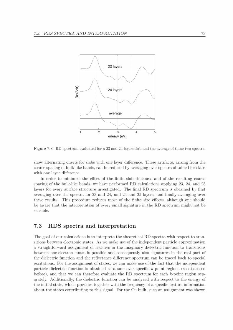
7.3. RDS SPECTRA AND INTERPRETATION 73
1 2 3 4 5
Re(
∆r/r
)
energy (eV)
23 layers
24 layers
average
Figure 7.8: RD spectrum evaluated for a 23 and 24 layers slab and the average of these two spectra.
show alternating onsets for slabs with one layer difference. These artifacts, arising from thecoarse spacing of bulk-like bands, can be reduced by averaging over spectra obtained for slabswith one layer difference.
In order to minimize the effect of the finite slab thickness and of the resulting coarsespacing of the bulk-like bands, we have performed RD calculations applying 23, 24, and 25layers for every surface structure investigated. The final RD spectrum is obtained by firstaveraging over the spectra for 23 and 24, and 24 and 25 layers, and finally averaging overthese results. This procedure reduces most of the finite size effects, although one shouldbe aware that the interpretation of every small signature in the RD spectrum might not besensible.
7.3 RDS spectra and interpretation
The goal of our calculations is to interprete the theoretical RD spectra with respect to tran-sitions between electronic states. As we make use of the independent particle approximationa straightforward assignment of features in the imaginary dielectric function to transitionsbetween one-electron states is possible and consequently also signatures in the real part ofthe dielectric function and the reflectance difference spectrum can be traced back to specialexcitations. For the assignment of states, we can make use of the fact that the independentparticle dielectric function is obtained as a sum over specific k-point regions (as discussedbefore), and that we can therefore evaluate the RD spectrum for each k-point region sep-arately. Additionally, the dielectric function can be analyzed with respect to the energy ofthe initial state, which provides together with the frequency of a specific feature informationabout the states contributing to this signal. For the Cu bulk, such an assignment was shown
74 CHAPTER 7. OPTICAL CALCULATIONS FOR CU(110) SURFACES
in Fig. 6.5. Combining these two techniques, an interpretation of the dielectric function ispossible. An assignment of RD features is slightly more complicated because not only thedifference between the imaginary dielectric function for x- and y- polarized light, but also thedifference in the real part contribute. These contributions are multiplied by the imaginaryand real part of the bulk dielectric function and everything is finally divided by the norm ofthe bulk dielectric function, so that the origin of RD feature is more obscure than for theimaginary dielectric function.
While an assignment of a transition with respect to the energy of the initial band and thek-point region is in principle unique, it is nevertheless useful to consider selection rules andgeneral properties of the band structure to disentangle possible transitions where the directmethod only provides information about regions of energy and k-points.
In a first step, one can assume that transition probabilities are unity for all possible(= energetically allowed) excitations [see Eq. (2.75)], and that the dielectric function onlydepends on the number of states available. In this approximation the contribution to thedielectric function from transitions between the occupied band v to the unoccupied band cis proportional to the corresponding joint density of states:
Jcv(ǫ) =
∫
BZ
2dk
(2π)3δ[ǫc(k) − ǫv(k)− ǫ]. (7.3)
Employing the properties of the δ-function, the density of states can be rewritten as a surfaceintegral
Jcv(ǫ) =2
(2π)3
∫
ǫc−ǫv=ǫ
dS
|∇k[ǫc(k)− ǫv(k)]|. (7.4)
Large contributions to the dielectric function therefore stem from ”flat” bands
∇k ǫc(k) = ∇k ǫv(k) = 0, (7.5)
occuring frequently at high symmetry points of the Brillouin zone. Also if two bands areparallel
∇k ǫc(k)−∇k ǫv(k) = 0, (7.6)
large contributions to the dielectric function can be expected.In the previous consideration, the transition probabilities were not explicitely taken into
account. For crystalline systems, group theory can be used to decide if transitions betweenbands at specific k-points are allowed according to their symmetry. For fcc and bcc bulklattices, such dipole transition tables can e.g., be found in Ref. [101]. For the interpretationof the dielectric function of the bare and the adsorbate covered Cu(110) surfaces we considerthe transition probabilities in an atomic like picture. To this end, the wavefunctions areprojected onto atomic orbitals and transitions analyzed in terms of elementary atomic dipoleselection rules. Such a procedure was e.g., applied by Smith [102] for the interpretationof the imaginary dielectric function of the Cu(111) and Cu(100) surface calculated with asimple semiempirical Hamiltonian. For electric dipole transitions the angular momentumnumber has to fulfill ∆l = ±1 (atomic dipole selection rule). Additionally, parity selectionrules allow only electron excitations between states with different parity with respect to the
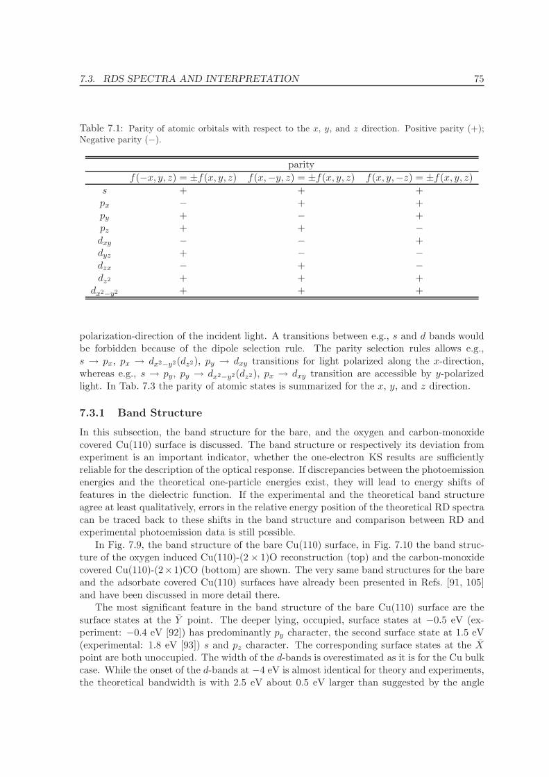
7.3. RDS SPECTRA AND INTERPRETATION 75
Table 7.1: Parity of atomic orbitals with respect to the x, y, and z direction. Positive parity (+);Negative parity (−).
parity
f(−x, y, z) = ±f(x, y, z) f(x,−y, z) = ±f(x, y, z) f(x, y,−z) = ±f(x, y, z)
s + + +px − + +py + − +pz + + −dxy − − +dyz + − −dzx − + −dz2 + + +
dx2−y2 + + +
polarization-direction of the incident light. A transitions between e.g., s and d bands wouldbe forbidden because of the dipole selection rule. The parity selection rules allows e.g.,s → px, px → dx2−y2(dz2), py → dxy transitions for light polarized along the x-direction,whereas e.g., s → py, py → dx2−y2(dz2), px → dxy transition are accessible by y-polarizedlight. In Tab. 7.3 the parity of atomic states is summarized for the x, y, and z direction.
7.3.1 Band Structure
In this subsection, the band structure for the bare, and the oxygen and carbon-monoxidecovered Cu(110) surface is discussed. The band structure or respectively its deviation fromexperiment is an important indicator, whether the one-electron KS results are sufficientlyreliable for the description of the optical response. If discrepancies between the photoemissionenergies and the theoretical one-particle energies exist, they will lead to energy shifts offeatures in the dielectric function. If the experimental and the theoretical band structureagree at least qualitatively, errors in the relative energy position of the theoretical RD spectracan be traced back to these shifts in the band structure and comparison between RD andexperimental photoemission data is still possible.
In Fig. 7.9, the band structure of the bare Cu(110) surface, in Fig. 7.10 the band struc-ture of the oxygen induced Cu(110)-(2× 1)O reconstruction (top) and the carbon-monoxidecovered Cu(110)-(2×1)CO (bottom) are shown. The very same band structures for the bareand the adsorbate covered Cu(110) surfaces have already been presented in Refs. [91, 105]and have been discussed in more detail there.
The most significant feature in the band structure of the bare Cu(110) surface are thesurface states at the Y point. The deeper lying, occupied, surface states at −0.5 eV (ex-periment: −0.4 eV [92]) has predominantly py character, the second surface state at 1.5 eV(experimental: 1.8 eV [93]) s and pz character. The corresponding surface states at the Xpoint are both unoccupied. The width of the d-bands is overestimated as it is for the Cu bulkcase. While the onset of the d-bands at −4 eV is almost identical for theory and experiments,the theoretical bandwidth is with 2.5 eV about 0.5 eV larger than suggested by the angle
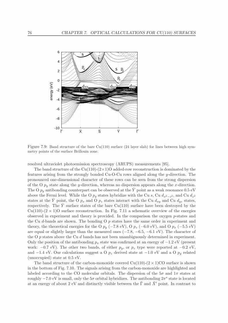
76 CHAPTER 7. OPTICAL CALCULATIONS FOR CU(110) SURFACES
-10
-8
-6
-4
-2
0
2
4
6
Γ X S Y Γ
yp
zps
xzd xydxyd
ss
xp
ener
gy (
eV)
Figure 7.9: Band structure of the bare Cu(110) surface (24 layer slab) for lines between high sym-metry points of the surface Brillouin zone.
resolved ultraviolet photoemission spectroscopy (ARUPS) measurements [95].
The band structure of the Cu(110)-(2×1)O added-row reconstruction is dominated by thefeatures arising from the strongly bonded Cu-O-Cu rows aligned along the y-direction. Thepronounced one-dimensional character of these rows can be seen from the strong dispersionof the O py state along the y-direction, whereas no dispersion appears along the x-direction.The O py antibonding counterpart can be observed at the Y point as a weak resonance 0.5 eVabove the Fermi level. While the O py states hybridize with the Cu s, Cu dx2−z2 , and Cu dz2
states at the Y point, the O px and O pz states interact with the Cu dxy and Cu dyz states,respectively. The Y surface states of the bare Cu(110) surface have been destroyed by theCu(110)-(2 × 1)O surface reconstruction. In Fig. 7.11 a schematic overview of the energiesobserved in experiment and theory is provided. In the comparison the oxygen p-states andthe Cu d-bands are shown. The bonding O p states have the same order in experiment andtheory, the theoretical energies for the O py (−7.8 eV), O pz (−6.0 eV), and O px (−5.5 eV)are equal or slightly larger than the measured ones (−7.8, −6.5, −6.1 eV). The character ofthe O p states above the Cu d bands has not been unambiguously determined in experiment.Only the position of the antibonding px state was confirmed at an energy of −1.2 eV (presentwork: −0.7 eV). The other two bands, of either py, or pz type were reported at −0.2 eV,and −1.4 eV. Our calculations suggest a O pz derived state at −1.0 eV and a O py related(unoccupied) state at 0.5 eV.
The band structure of the carbon-monoxide covered Cu(110)-(2× 1)CO surface is shownin the bottom of Fig. 7.10. The signals arising from the carbon-monoxide are highlighted andlabeled according to the CO molecular orbitals. The dispersion of the 5σ and 1π states atroughly −7.0 eV is small, only the 5σ orbital hybridizes. The antibonding 2π∗ state is locatedat an energy of about 2 eV and distinctly visible between the Γ and X ′ point. In contrast to
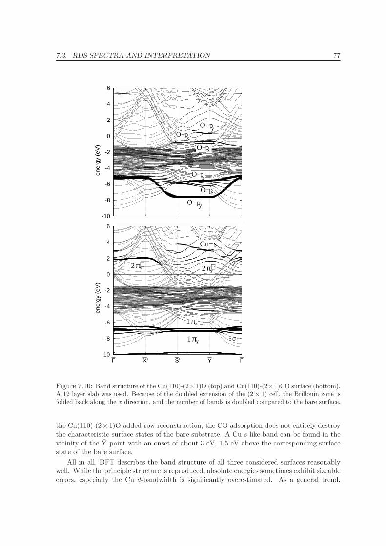
7.3. RDS SPECTRA AND INTERPRETATION 77
-10
-8
-6
-4
-2
0
2
4
6
GYS’X’G
-10
-8
-6
-4
-2
0
2
4
6
ΓYS’X’Γ
O−zp
O− zp
O−x
pO− yp
O−xp
O− yp
1πy
1πx
σ5
π2 ∗y
sCu−
π2 ∗y
ener
gy (
eV)
ener
gy (
eV)
Figure 7.10: Band structure of the Cu(110)-(2×1)O (top) and Cu(110)-(2×1)CO surface (bottom).A 12 layer slab was used. Because of the doubled extension of the (2 × 1) cell, the Brillouin zone isfolded back along the x direction, and the number of bands is doubled compared to the bare surface.
the Cu(110)-(2×1)O added-row reconstruction, the CO adsorption does not entirely destroythe characteristic surface states of the bare substrate. A Cu s like band can be found in thevicinity of the Y point with an onset of about 3 eV, 1.5 eV above the corresponding surfacestate of the bare surface.
All in all, DFT describes the band structure of all three considered surfaces reasonablywell. While the principle structure is reproduced, absolute energies sometimes exhibit sizeableerrors, especially the Cu d-bandwidth is significantly overestimated. As a general trend,
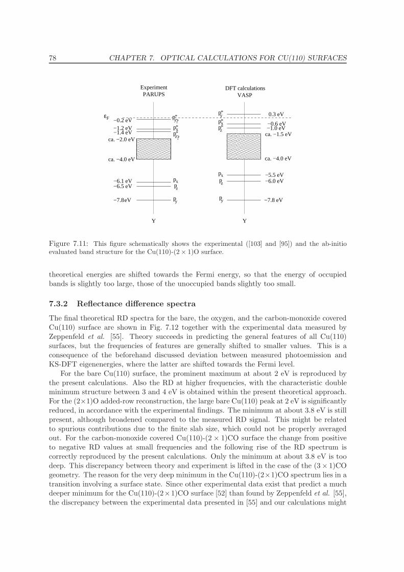
78 CHAPTER 7. OPTICAL CALCULATIONS FOR CU(110) SURFACES
pz
px
py
pz*
px*
py*
py
pz
px
pz*
px*
py*
−7.8 eV
εF
Y Y
−6.5 eV −6.1 eV
ca. −4.0 eV
ca. −2.0 eV−1.4 eV−1.2 eV
−7.8 eV
−6.0 eV−5.5 eV
ca. −4.0 eV
ca. −1.5 eV−1.0 eV −0.6 eV
0.3 eV
?
?
ExperimentPARUPS VASP
−0.2 eV
DFT calculations
Figure 7.11: This figure schematically shows the experimental ([103] and [95]) and the ab-initioevaluated band structure for the Cu(110)-(2× 1)O surface.
theoretical energies are shifted towards the Fermi energy, so that the energy of occupiedbands is slightly too large, those of the unoccupied bands slightly too small.
7.3.2 Reflectance difference spectra
The final theoretical RD spectra for the bare, the oxygen, and the carbon-monoxide coveredCu(110) surface are shown in Fig. 7.12 together with the experimental data measured byZeppenfeld et al. [55]. Theory succeeds in predicting the general features of all Cu(110)surfaces, but the frequencies of features are generally shifted to smaller values. This is aconsequence of the beforehand discussed deviation between measured photoemission andKS-DFT eigenenergies, where the latter are shifted towards the Fermi level.
For the bare Cu(110) surface, the prominent maximum at about 2 eV is reproduced bythe present calculations. Also the RD at higher frequencies, with the characteristic doubleminimum structure between 3 and 4 eV is obtained within the present theoretical approach.For the (2×1)O added-row reconstruction, the large bare Cu(110) peak at 2 eV is significantlyreduced, in accordance with the experimental findings. The minimum at about 3.8 eV is stillpresent, although broadened compared to the measured RD signal. This might be relatedto spurious contributions due to the finite slab size, which could not be properly averagedout. For the carbon-monoxide covered Cu(110)-(2 × 1)CO surface the change from positiveto negative RD values at small frequencies and the following rise of the RD spectrum iscorrectly reproduced by the present calculations. Only the minimum at about 3.8 eV is toodeep. This discrepancy between theory and experiment is lifted in the case of the (3× 1)COgeometry. The reason for the very deep minimum in the Cu(110)-(2×1)CO spectrum lies in atransition involving a surface state. Since other experimental data exist that predict a muchdeeper minimum for the Cu(110)-(2×1)CO surface [52] than found by Zeppenfeld et al. [55],the discrepancy between the experimental data presented in [55] and our calculations might
7.3. RDS SPECTRA AND INTERPRETATION 79
1 2 3 4 1 2 3 4 5
Re(
∆r/r
)
energy (eV)
theory experiment
Cu(110)−(2x1)CO
Cu(110)−(2x1)O
bare Cu(110)
Cu(110)−(3x1)CO
Figure 7.12: RD spectra for the bare, the oxygen induced Cu(110)-(2×1)O added-row reconstruction,the carbon-monoxide covered Cu(110)-(2 × 1)CO and Cu(110)-(3 × 1)CO surface. The theoreticalspectra (left) are compared to the experimental results [55].
be related to a non-perfectly ordered experimental surface structure. On the other hand, animprecise theoretical description of the relative position of the surface state can not be ruledout.
In the following, we will derive the origin of the main RD features by analyzing the energyand k-point origin of specific transitions. For the bare Cu(110) surface (see Fig. 7.13) themost prominent features of the RD spectrum is the large maximum at energies of about2 eV and the double minimum structure at larger frequencies, where the second minimumoccurs for all Cu(110) surfaces independently of the present adsorbate. The large maximumat about 2 eV was assumed to be connected to the characteristic bare Cu(110) surface statesat the Y point [52, 53, 58, 59, 60]. We find that transitions between the occupied surfacestate with py character and the unoccupied surface state with s character are indeed themain source for this strong absorption for y-polarized light. But in addition to this surfacestate − surface state transition, the final shape of this peak is determined by transitionsfrom dxy like bands at the top of the Cu d-bands to px states at the Fermi level near the Xpoint (positive RD contribution), and transitions to py like states between the Γ and Y point(negative RD contribution). In total these transitions result in a small positive RD shoulderat about 2 eV, as already proposed by Sun et al. [58]
The RD minimum at about 3.8 eV, which occurs for all Cu(110) surfaces studied inthe present work, is not related to specific surface states but arises from the anisotropy ofthe Cu(110) surface itself. The origin of this minimum lies in transitions in the vicinityof the S point from px and py like states at the Fermi energy to an unoccupied s-band atabout 3.8 eV. Due to the fact that the surface contribution of px like orbitals is significantlystronger, the net absorption strength is larger (by about a factor of 2) for light polarized
80 CHAPTER 7. OPTICAL CALCULATIONS FOR CU(110) SURFACES
-12
-8
-4
0
4
8
12
1 2 3 4 5
Re(
∆r/r
)
energy (eV)
dxy px
Xat
dxy py Γ Yat ,
px
spy
sSat
dxz surface state s Ypz
at
py
s Yatsurface state−surface state
Figure 7.13: RD spectrum of the bare Cu(110) surface. Significant contributions are explicitelyindicated.
-12
-8
-4
0
4
8
12
1 2 3 4 5
Re(
∆r/r
)
energy (eV)
py
py
OCu
py
dz²CuCudx²−y²
( Cu )
px
spy
sSat
py
O
pz
py
O O
pz
(1x1)
( Cu Cu )yzd
xzdCu
Figure 7.14: RD spectrum of the oxygen induced Cu(110)-(2× 1)O added-row reconstruction andsignificant contributions to it.
along the x direction. The reason for this minimum is therefore not the different energyonset for the transitions from px and py states as proposed by Zeppenfeld et al. [54], but thedifference in the absorption strength for these bands with different symmetry. Because the
7.3. RDS SPECTRA AND INTERPRETATION 81
-12
-8
-4
0
4
8
12
1 2 3 4 5
Re(
∆r/r
)
energy (eV)
py s Ysurface state at
px
spy
sSat (1x1)
derivative model
Figure 7.15: RD spectrum of the carbon monoxide covered Cu(110)-(2×1)CO surface and significantcontributions to it.
contributing bands do not change with adsorption, the minimum at about 3.8 eV is presentfor all considered surfaces.
The last feature not yet explained for the bare Cu(110) surface is the second minimumat about 3 eV. It is another signature of the unoccupied surface state at the Y point, withthe initial state of dxz character situated at the top of the Cu d-bands. The transitionprobabilities are not vanishing, due to the s and pz character of the unoccupied surfacestate.
For both, the (2 × 1)O and (2 × 1)CO surface, the large maximum at 2 eV vanishes,to be replaced by a much smaller positive RD signal for the (2 × 1)O, and even a negativesignature for the (2×1)CO surface. While for the (2×1)O surface states associated with theadsorbed oxygen are responsible for the RD form at small frequencies, as will be shown later,the (2×1)CO surface seems not to be influenced by specific transitions but by a general shiftof the dielectric function for light polarized along x- and y- direction. This shift amounts toabout +0.08 eV for y polarized light, so that the absorption in x-direction sets in slightlyearlier causing the negative sign of the RD spectrum. Such a behavior can be explained bya derivative model [104]. For the (2 × 1)O surface, this shift is overlaid by transitions tothe unoccupied O py state at about 0.5 eV, with additional Cu dx2−y2 , Cu dz2, and Cu pz
character. Three different contributions can be observed: transitions from the O pz stateat −1.0 eV to the O py state (positive RD contribution), transitions from Cu py like statesat energies between −1.5 and −1.0 eV to the O py state (positive RD contribution), andtransitions from Cu dxz states slightly above the Cu d-bands (≈ −1.5 eV) to the O py state(negative RD contribution). The last contribution gives rise to the small minimum at about2 eV.
82 CHAPTER 7. OPTICAL CALCULATIONS FOR CU(110) SURFACES
The Cu(110)-(2× 1)O and Cu(110)-(2× 1)CO RD spectra at higher frequencies are bothdominated by the minimum at 3.8 eV described above. For the Cu(110)-(2 × 1)CO surface,this minimum is additionally deepened compared to the other surfaces. We found that thisdeepened minimum results from an additional transition between Cu-py bulklike states to a(2×1)CO Y surface state at about 3 eV. This state has the same character as the unoccupiedsurface state of the bare Cu(110) surface (s-type), but is situated at a larger energy (3 eVcompared to 1.5 eV for the bare surface), resulting in an absorption peak for y-polarizedlight at about 3.4 eV. In the RD, this feature manifests itself as a minimum around 3.7 eV.The negative sign of the RD contribution results from the increased importance of the realpart of the surface dielectric anisotropy, as the imaginary part of the bulk dielectric functionbecomes larger than the respective real one.
The deviations between theoretical and experimental RD spectra concerning the depthof the minimum at 3.8 eV is lifted for the case of the Cu(110)-(3 × 1)CO surface. Thedepth of the minimum is now in agreement with the experimental data (see Ref. [55] andFig. 7.12). Experiments suggest that the minimum at about 3.8 eV is very sensitive to surfacedefects and the roughness of the surface. The neglect of these contributions in the theoreticaldescription of the RD (2 × 1)CO spectrum, respectively, a quenching of the surface statesby the roughened surface in experiments, might lead to the deviation for the depth of theminimum.
Chapter 8
Conclusions and Summary
This part of my thesis has been focused on the calculation of the reflectance difference spectrafor the bare Cu(110), the oxygen covered Cu(110)-(2×1)O, and the carbon-monoxide coveredCu(110)-(2 × 1)CO and Cu(110)-(3 × 1)CO surfaces. The Cu(110) substrate was chosenbecause it is among the best studied metallic surfaces using RD spectroscopy and numerousof these measurements have been performed by our collaborators Peter Zeppenfeld and co-workers at the University of Linz [54, 55, 56, 57, 58].
The evaluation of the reflectance difference spectrum requires the (anisotropic) dielectricfunction of the considered surface as well as the optical response of the bulk material. Be-sides giving the RD spectrum, the present calculations were therefore also among the firstapplications of the PAW optical routines within the VASP code [21] for bulk metals as wellas for the optical response of surfaces. For the correct description of the dielectric function ofmetallic systems, the expression for the intraband plasma frequency has been implementedin the VASP code, and was tested for various metallic systems in Sec. 6.1. The relationshipbetween intraband transitions and interband transitions at small frequencies has been em-phasized in subsection 7.2.3, and convergence tests for the surface dielectric function havebeen outlined in Sec. 7.2.
As the RD spectrum depends on the real and imaginary part of the bulk and surfacedielectric function in a non-trivial way, the interpretation of the experimental RD spectrawith respect to specific transitions is not straightforward. Therefore, an ab-initio calcula-tion of the RD spectrum and the interpretation of this spectrum in terms of the underlyingelectronic transitions is of interest. In the independent particle approximation, which weused to describe the dielectric function, light can only be absorbed, if the frequency of thelight corresponds to the energy difference between two one-electron eigenenergies. Agree-ment with experiment can only be expected if the one-electron eigenenergies correspondto the quasi-particle energies as measured in (inverse) photoemission spectroscopy. Bandstructure calculations for all considered Cu(110) surfaces and the comparison to experimenthave been presented in subsection 7.3.1. We find that bulk like bands, surface states, andadsorbate associated features are in qualitative agreement with the experimental findings,although the theoretical one-particle energies are generally shifted towards the Fermi energyresulting in red-shifted dielectric functions and RD spectra. As we have shown in Sec. 9.1,GW calculations would improve the Cu bandstructure in some aspects, but unfortunatelylarge scale calculations for enough k-points are yet not possible using GW due to the large
83
84 CHAPTER 8. CONCLUSIONS AND SUMMARY
computational effort included.For all Cu(110) surfaces, independent on the specific adsorbate, Zeppenfeld and co-
workers find an RD minimum at an energy of about 4.4 eV. This feature, situated at 3.8 eVin the theoretical spectra, can be explained by transitions from p-like states near the Fermienergy to an unoccupied bulk-like s state at the S point. Due to the surface anisotropy, thepx character is stronger at this high symmetry point favoring absorption for light polarizedalong the x-direction. For the bare Cu(110) surface, the importance of the surface statesfor the RD could be confirmed. In the case of the oxygen covered surface, oxygen associ-ated states are responsible for the RD maximum and the subsequent minimum in the lowfrequency range (1.5−2.5 eV). A surface state is found to be the reason for the deepened 3.8eV minimum of the theoretical Cu(110)-(2×1)CO structure, not present in the experimentalspectrum. We think that this discrepancy might be related to a quenching of the surfacestate by disorder in the experimental setup.
For the Cu(110) bare, oxygen and carbon-monoxide covered surfaces, we find that theindependent particle approximation provides a reasonable description of the surface opticalresponse. The main features of the experimental RD spectra are reproduced but shifted tosmaller energies. The RD spectra have been published in Ref. [105].
Part III
GW calculations
85
Chapter 9
Quasiparticle energies for metals
In the third part of my thesis, I will present GW quasiparticle calculations for d-metals, thenoble metals Cu, Ag, and the magnetic transitions metals Fe and Ni. Our results will be com-pared to previous calculations by other groups. An introduction to GW and to the evaluationof quasiparticle energies has been given in chapter 4. More details about the implementationof the GW routines in VASP and quasiparticle energies for semiconductors and insulatorscan be found in Refs. [25, 48]. The difference between semiconductors/insulators and metalsis the existence of partially filled bands in the case of metals. This implies two importantdifferences for the quasiparticle calculations of semiconductor/insulators and metals: First,the k-point convergence of the total quasiparticle energies is slower than for insulators, be-cause it involves the calculation of the Fermi energy, which converges slowly with the numberof k-points. Secondly, intraband transitions contribute to the dielectric function ε(q). Forthe long-wavelength limit q → 0, the intraband contribution is determined by the plasmafrequency [Eq. (2.113)]. In order to take the long-wavelength intraband contributions intoaccount, we evaluate the plasma frequency and add the corresponding Drude term to theinterband dielectric function. If one does not include the Drude term, one neglects importantcontributions at the Γ point and thus a large number of q-points would be required.
In all quasiparticle calculations presented in this chapter we have used GW potentials.As a larger number of unoccupied bands are required for the GW calculations (and also forthe ACFDT calculations presented in part IV of this thesis), it is important that the PAWpseudopotentials describe also the scattering properties of empty states accurately. Thereforespecial GW potentials are generated which reproduce the scattering properties of a sphericalreference atom up to ≈ 10 Ry exactly. Details concerning the PAW potentials used in thischapter are summerized in Tab. 9.1.
9.1 Noble metals - Cu and Ag
In the following we will present G0W0 quasiparticle energies for the noble metals Cu andAg. Both Cu and Ag crystallize in an fcc structure with an experimental lattice constantof 3.615 A and 4.086 A, respectively. The d-bands are fully occupied with the highest DFTd-states1 found at −1.56 eV and −2.74 eV for Cu and Ag, respectively, which is about 0.5
1The band structures obtained applying the LDA or the PBE exchange-correlation potential are verysimilar for the noble metals.
86
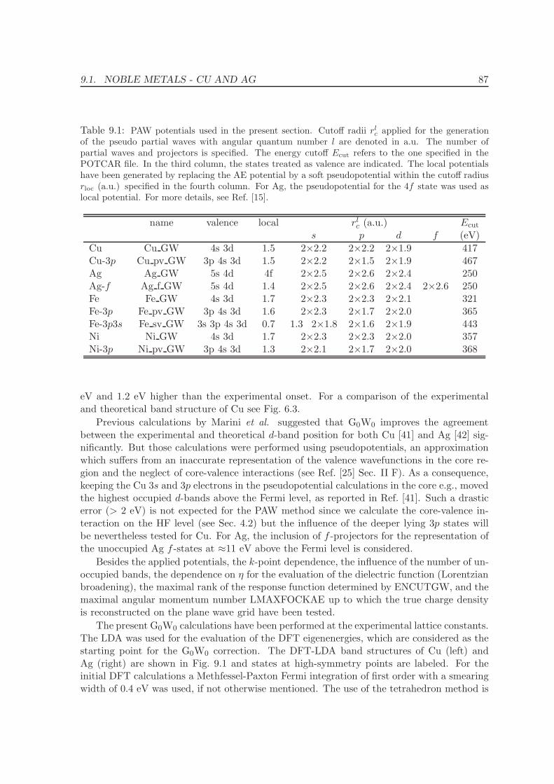
9.1. NOBLE METALS - CU AND AG 87
Table 9.1: PAW potentials used in the present section. Cutoff radii rlc applied for the generation
of the pseudo partial waves with angular quantum number l are denoted in a.u. The number ofpartial waves and projectors is specified. The energy cutoff Ecut refers to the one specified in thePOTCAR file. In the third column, the states treated as valence are indicated. The local potentialshave been generated by replacing the AE potential by a soft pseudopotential within the cutoff radiusrloc (a.u.) specified in the fourth column. For Ag, the pseudopotential for the 4f state was used aslocal potential. For more details, see Ref. [15].
name valence local rlc (a.u.) Ecut
s p d f (eV)
Cu Cu GW 4s 3d 1.5 2×2.2 2×2.2 2×1.9 417Cu-3p Cu pv GW 3p 4s 3d 1.5 2×2.2 2×1.5 2×1.9 467Ag Ag GW 5s 4d 4f 2×2.5 2×2.6 2×2.4 250Ag-f Ag f GW 5s 4d 1.4 2×2.5 2×2.6 2×2.4 2×2.6 250Fe Fe GW 4s 3d 1.7 2×2.3 2×2.3 2×2.1 321Fe-3p Fe pv GW 3p 4s 3d 1.6 2×2.3 2×1.7 2×2.0 365Fe-3p3s Fe sv GW 3s 3p 4s 3d 0.7 1.3 2×1.8 2×1.6 2×1.9 443Ni Ni GW 4s 3d 1.7 2×2.3 2×2.3 2×2.0 357Ni-3p Ni pv GW 3p 4s 3d 1.3 2×2.1 2×1.7 2×2.0 368
eV and 1.2 eV higher than the experimental onset. For a comparison of the experimentaland theoretical band structure of Cu see Fig. 6.3.
Previous calculations by Marini et al. suggested that G0W0 improves the agreementbetween the experimental and theoretical d-band position for both Cu [41] and Ag [42] sig-nificantly. But those calculations were performed using pseudopotentials, an approximationwhich suffers from an inaccurate representation of the valence wavefunctions in the core re-gion and the neglect of core-valence interactions (see Ref. [25] Sec. II F). As a consequence,keeping the Cu 3s and 3p electrons in the pseudopotential calculations in the core e.g., movedthe highest occupied d-bands above the Fermi level, as reported in Ref. [41]. Such a drasticerror (> 2 eV) is not expected for the PAW method since we calculate the core-valence in-teraction on the HF level (see Sec. 4.2) but the influence of the deeper lying 3p states willbe nevertheless tested for Cu. For Ag, the inclusion of f -projectors for the representation ofthe unoccupied Ag f -states at ≈11 eV above the Fermi level is considered.
Besides the applied potentials, the k-point dependence, the influence of the number of un-occupied bands, the dependence on η for the evaluation of the dielectric function (Lorentzianbroadening), the maximal rank of the response function determined by ENCUTGW, and themaximal angular momentum number LMAXFOCKAE up to which the true charge densityis reconstructed on the plane wave grid have been tested.
The present G0W0 calculations have been performed at the experimental lattice constants.The LDA was used for the evaluation of the DFT eigenenergies, which are considered as thestarting point for the G0W0 correction. The DFT-LDA band structures of Cu (left) andAg (right) are shown in Fig. 9.1 and states at high-symmetry points are labeled. For theinitial DFT calculations a Methfessel-Paxton Fermi integration of first order with a smearingwidth of 0.4 eV was used, if not otherwise mentioned. The use of the tetrahedron method is
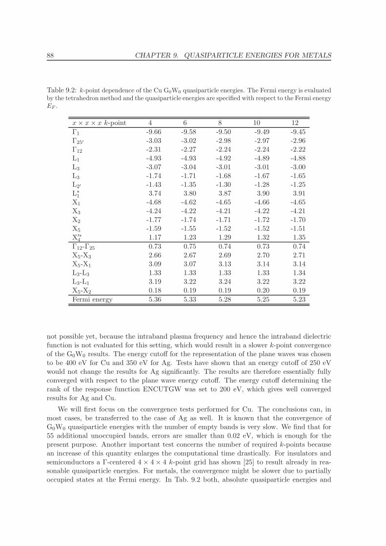
88 CHAPTER 9. QUASIPARTICLE ENERGIES FOR METALS
Table 9.2: k-point dependence of the Cu G0W0 quasiparticle energies. The Fermi energy is evaluatedby the tetrahedron method and the quasiparticle energies are specified with respect to the Fermi energyEF .
x× x× x k-point 4 6 8 10 12
Γ1 -9.66 -9.58 -9.50 -9.49 -9.45Γ25′ -3.03 -3.02 -2.98 -2.97 -2.96Γ12 -2.31 -2.27 -2.24 -2.24 -2.22L1 -4.93 -4.93 -4.92 -4.89 -4.88L3 -3.07 -3.04 -3.01 -3.01 -3.00L3 -1.74 -1.71 -1.68 -1.67 -1.65L2′ -1.43 -1.35 -1.30 -1.28 -1.25L∗
1 3.74 3.80 3.87 3.90 3.91X1 -4.68 -4.62 -4.65 -4.66 -4.65X3 -4.24 -4.22 -4.21 -4.22 -4.21X2 -1.77 -1.74 -1.71 -1.72 -1.70X5 -1.59 -1.55 -1.52 -1.52 -1.51X′∗
4 1.17 1.23 1.29 1.32 1.35
Γ12-Γ25 0.73 0.75 0.74 0.73 0.74X5-X3 2.66 2.67 2.69 2.70 2.71X5-X1 3.09 3.07 3.13 3.14 3.14L3-L3 1.33 1.33 1.33 1.33 1.34L3-L1 3.19 3.22 3.24 3.22 3.22X5-X2 0.18 0.19 0.19 0.20 0.19
Fermi energy 5.36 5.33 5.28 5.25 5.23
not possible yet, because the intraband plasma frequency and hence the intraband dielectricfunction is not evaluated for this setting, which would result in a slower k-point convergenceof the G0W0 results. The energy cutoff for the representation of the plane waves was chosento be 400 eV for Cu and 350 eV for Ag. Tests have shown that an energy cutoff of 250 eVwould not change the results for Ag significantly. The results are therefore essentially fullyconverged with respect to the plane wave energy cutoff. The energy cutoff determining therank of the response function ENCUTGW was set to 200 eV, which gives well convergedresults for Ag and Cu.
We will first focus on the convergence tests performed for Cu. The conclusions can, inmost cases, be transferred to the case of Ag as well. It is known that the convergence ofG0W0 quasiparticle energies with the number of empty bands is very slow. We find that for55 additional unoccupied bands, errors are smaller than 0.02 eV, which is enough for thepresent purpose. Another important test concerns the number of required k-points becausean increase of this quantity enlarges the computational time drastically. For insulators andsemiconductors a Γ-centered 4 × 4 × 4 k-point grid has shown [25] to result already in rea-sonable quasiparticle energies. For metals, the convergence might be slower due to partiallyoccupied states at the Fermi energy. In Tab. 9.2 both, absolute quasiparticle energies and
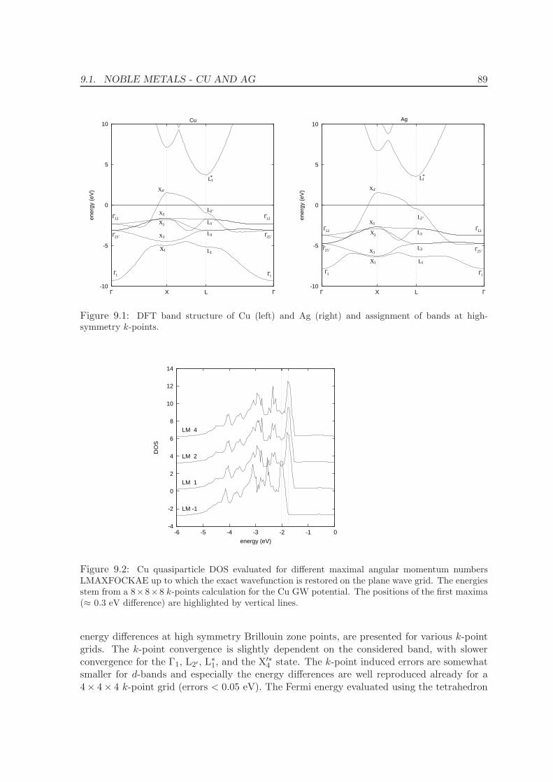
9.1. NOBLE METALS - CU AND AG 89
-10
-5
0
5
10
ΓLXΓ
ener
gy (
eV)
Γ1
Γ12
Γ25’
Γ1
Γ25’
Γ12
X1
X3
X2
X5
X4’
L1
L3
L3
L2’
L1
Cu
*
-10
-5
0
5
10
ΓLXΓen
ergy
(eV
)
Γ1Γ1
X4’
L1
Γ25’ Γ25’
Γ12Γ12
X1
X3
X2
X5
L1
L3
L3
L2’
Ag
*
Figure 9.1: DFT band structure of Cu (left) and Ag (right) and assignment of bands at high-symmetry k-points.
-4
-2
0
2
4
6
8
10
12
14
-6 -5 -4 -3 -2 -1 0
DO
S
energy (eV)
LM -1
LM 1
LM 2
LM 4
Figure 9.2: Cu quasiparticle DOS evaluated for different maximal angular momentum numbersLMAXFOCKAE up to which the exact wavefunction is restored on the plane wave grid. The energiesstem from a 8×8×8 k-points calculation for the Cu GW potential. The positions of the first maxima(≈ 0.3 eV difference) are highlighted by vertical lines.
energy differences at high symmetry Brillouin zone points, are presented for various k-pointgrids. The k-point convergence is slightly dependent on the considered band, with slowerconvergence for the Γ1, L2′ , L∗
1, and the X′∗4 state. The k-point induced errors are somewhat
smaller for d-bands and especially the energy differences are well reproduced already for a4× 4× 4 k-point grid (errors < 0.05 eV). The Fermi energy evaluated using the tetrahedron
90 CHAPTER 9. QUASIPARTICLE ENERGIES FOR METALS
method seems to converge faster than the Fermi energy obtained applying the Methfessel-Paxton smearing, so that we use the tetrahedron method for the evaluation of the G0W0
Fermi energy throughout this work. But it should be kept in mind, that even applying thetetrahedron method the Fermi energy for a 8 × 8 × 8 k-point grid (both for DFT and GW)is not better converged than ≈ 0.06 eV. Differences between 12 × 12 × 12 and 10 × 10 × 10results are however well below 50 meV, for most energies below 20 meV, which suffices forthe present purpose.
Further tests show that the G0W0 quasiparticle energies are hardly affected by choosingthe smearing width 0.2 or 0.4 eV in the initial DFT calculation. Furthermore, reducing theimaginary shift η for the evaluation of the self energy and the polarizability from 0.1 eV to0.01 eV leads to almost no change in the quasiparticle energies. Only the X1 state is shiftedupwards by 0.06 eV. The largest effect on the quasiparticle energies, nevertheless, is causedby the introduction or the neglect, respectively, of LMAXFOCKAE. By setting LMAX-FOCKAE to an angular momentum number l, all components of the difference between AEand PS partial densities up to this momentum are reconstructed on a plane wave grid andconsequently the form of the AE density is approximately reconstructed (see Sec. 2.7). InFig. 9.2 the Cu G0W0 density of states obtained neglecting the AE reconstruction (LM −1),and results for increasing values of LMAXFOCKAE are shown. If the form of the AE den-sity is not recovered, the topmost d-bands start at lower energies (the first maximum of thed-bands is highlighted by a vertical line) resulting in a reduction of the bandwidth from 3.3eV with LMAXFOCKAE = 4 to 3.0 eV for LMAXFOCKAE = −1. Although the positionof the d-bands agrees better with experiment if LMAXFOCKAE = −1, this is an artefactof the crude approximation of the exact charge density. Interestingly, the results stemmingfrom setting the maximal angular momentum to 1 or 4 do not differ much. For the heavierAg, the difference between considering the AE reconstruction or not is much smaller thanfor Cu. The reason for these observations is that the exact Cu 3d wavefunctions are spatiallystrongly contracted, and VASP usually only attempts to restore the moments of the chargedensity without any consideration of the exact shape of the 3d wavefunctions. This causes anoverestimation of the 3d-3d screened exchange interaction. By restoring the correct spatialcharge distribution on the plane wave grid, the screened exchange interaction is well approx-imated. These issues are less critical for 4d states, which are spatially less contracted, thusthe Ag results are less dependent on LMAXFOCKAE.
In Tab. 9.3 the Cu G0W0 quasiparticle energies obtained for two different Cu potentials,one without, one with the 3p electrons included in the valence, are shown. A 12 × 12 × 12k-point grid and LMAXFOCKAE = 4 were applied. Additionally, the energies calculated byMarini et al. [41] employing a pseudopotential plane wave code and by Zhukov et al. [106]using the full potential LMTO approximation are presented. We first note that LDA resultsare little changed by the choice of the PAW potential, whereas the GW results depend on thetreatment of the 3p electrons. The most significant error in the DFT one-electron energiesis the wrong description of the absolute position and the bandwidth of the d-states. Thehighest d-band (see X5 state) is located at −1.56 eV in LDA, whereas experiments suggest−2.01 eV, a difference of 0.45 eV. The error in the low energy d onset (see X1) is smaller(0.2 eV), so that, as a consequence, the bandwidth (in Tab. 9.3 in italic letters) is 3.42 eVin DFT versus 3.17 eV in experiment. Unfortunately, our G0W0 results can not correct thisbehavior and the uppermost d-bands are shifted to even slightly higher energies (about 0.1
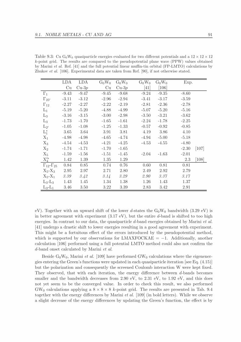
9.1. NOBLE METALS - CU AND AG 91
Table 9.3: Cu G0W0 quasiparticle energies evaluated for two different potentials and a 12× 12× 12k-point grid. The results are compared to the pseudopotential plane wave (PPW) values obtainedby Marini et al. Ref. [41] and the full potential linear muffin-tin orbital (FP-LMTO) calculations byZhukov et al. [106]. Experimental data are taken from Ref. [90], if not otherwise stated.
LDA LDA G0W0 G0W0 G0W0 G0W0 Exp.Cu Cu-3p Cu Cu-3p [41] [106]
Γ1 -9.43 -9.47 -9.45 -9.68 -9.24 -9.35 -8.60Γ25′ -3.11 -3.12 -2.96 -2.94 -3.41 -3.17 -3.59Γ12 -2.27 -2.27 -2.22 -2.19 -2.81 -2.36 -2.78L1 -5.19 -5.20 -4.88 -4.99 -5.07 -5.20 -5.16L3 -3.16 -3.15 -3.00 -2.98 -3.50 -3.21 -3.62L3 -1.73 -1.70 -1.65 -1.61 -2.24 -1.78 -2.25L2′ -1.05 -1.08 -1.25 -1.33 -0.57 -0.92 -0.85L∗
1 3.65 3.64 3.91 3.81 4.19 3.86 4.10X1 -4.98 -4.98 -4.65 -4.74 -4.94 -5.00 -5.18X3 -4.54 -4.53 -4.21 -4.25 -4.53 -4.55 -4.80X2 -1.74 -1.71 -1.70 -1.65 -2.30 [107]X5 -1.59 -1.56 -1.51 -1.45 -2.04 -1.63 -2.01X′∗
4 1.42 1.39 1.35 1.29 2.3 [108]
Γ12-Γ25 0.84 0.85 0.74 0.76 0.60 0.81 0.81X5-X3 2.95 2.97 2.71 2.80 2.49 2.92 2.79X5-X1 3.39 3.42 3.14 3.29 2.90 3.37 3.17L3-L3 1.43 1.45 1.34 1.38 1.26 1.43 1.37L3-L1 3.46 3.50 3.22 3.39 2.83 3.42 2.91
eV). Together with an upward shift of the lower d-states the G0W0 bandwidth (3.29 eV) isin better agreement with experiment (3.17 eV), but the entire d-band is shifted to too highenergies. In contrast to our data, the quasiparticle d-band energies obtained by Marini et al.[41] undergo a drastic shift to lower energies resulting in a good agreement with experiment.This might be a fortuitous effect of the errors introduced by the pseudopotential method,which is supported by our observations for LMAXFOCKAE = −1. Additionally, anothercalculation [106] performed using a full potential LMTO method could also not confirm thed-band onset calculated by Marini et al.
Beside G0W0, Marini et al. [109] have performed GW0 calculations where the eigenener-gies entering the Green’s functions were updated in each quasiparticle iteration [see Eq. (4.15)]but the polarization and consequently the screened Coulomb interaction W were kept fixed.They observed, that with each iteration, the energy difference between d-bands becomessmaller and the bandwidth decreases from 2.90 eV, to 2.31 eV, to 1.92 eV, and this doesnot yet seem to be the converged value. In order to check this result, we also performedGW0 calculations applying a 8 × 8 × 8 k-point grid. The results are presented in Tab. 9.4together with the energy differences by Marini et al. [109] (in bold letters). While we observea slight decrease of the energy differences by updating the Green’s function, the effect is by
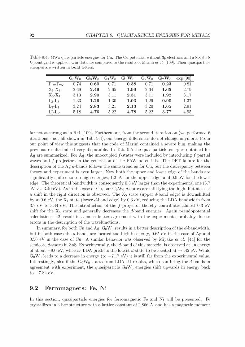
92 CHAPTER 9. QUASIPARTICLE ENERGIES FOR METALS
Table 9.4: GW0 quasiparticle energies for Cu. The Cu potential without 3p electrons and a 8×8×8k-point grid is applied. Our data are compared to the results of Marini et al. [109]. Their quasiparticleenergies are written in bold letters.
G0W0 G0W0 G1W0 G1W0 G2W0 G2W0 exp.[90]
Γ12-Γ25′ 0.74 0.60 0.71 0.38 0.71 0.23 0.81X5-X3 2.69 2.49 2.65 1.99 2.64 1.65 2.79X5-X1 3.13 2.90 3.11 2.31 3.11 1.92 3.17L3-L3 1.33 1.26 1.30 1.03 1.29 0.90 1.37L3-L1 3.24 2.83 3.21 2.13 3.20 1.65 2.91L∗
1-L2′ 5.18 4.76 5.22 4.78 5.22 3.77 4.95
far not as strong as in Ref. [109]. Furthermore, from the second iteration on (we performed 6iterations - not all shown in Tab. 9.4), our energy differences do not change anymore. Fromour point of view this suggests that the code of Marini contained a severe bug, making theprevious results indeed very disputable. In Tab. 9.5 the quasiparticle energies obtained forAg are summarized. For Ag, the unoccupied f -states were included by introducing f partialwaves and f -projectors in the generation of the PAW potentials. The DFT failure for thedescription of the Ag d-bands follows the same trend as for Cu, but the discrepancy betweentheory and experiment is even larger. Now both the upper and lower edge of the bands aresignificantly shifted to too high energies, 1.2 eV for the upper edge, and 0.9 eV for the loweredge. The theoretical bandwidth is consequently 0.3 eV larger than the experimental one (3.7eV vs. 3.40 eV). As in the case of Cu, our G0W0 d-states are still lying too high, but at leasta shift in the right direction is observed. The X5 state (upper d-band edge) is downshiftedby ≈ 0.6 eV, the X1 state (lower d-band edge) by 0.3 eV, reducing the LDA bandwidth from3.7 eV to 3.44 eV. The introduction of the f -projector thereby contributes almost 0.3 eVshift for the X5 state and generally decreases the d-band energies. Again pseudopotentialcalculations [42] result in a much better agreement with the experiments, probably due toerrors in the description of the wavefunctions.
In summary, for both Cu and Ag, G0W0 results in a better description of the d-bandwidth,but in both cases the d-bands are located too high in energy, 0.65 eV in the case of Ag and0.56 eV in the case of Cu. A similar behavior was observed by Miyake et al. [44] for thesemicore d-states in ZnS. Experimentally, the d-band of this material is observed at an energyof about −9.0 eV, whereas LDA predicts the lowest d-state to be located at −6.42 eV. WhileG0W0 leads to a decrease in energy (to −7.17 eV) it is still far from the experimental value.Interestingly, also if the G0W0 starts from LDA+U results, which can bring the d-bands inagreement with experiment, the quasiparticle G0W0 energies shift upwards in energy backto −7.82 eV.
9.2 Ferromagnets: Fe, Ni
In this section, quasiparticle energies for ferromagnetic Fe and Ni will be presented. Fecrystallizes in a bcc structure with a lattice constant of 2.866 A and has a magnetic moment
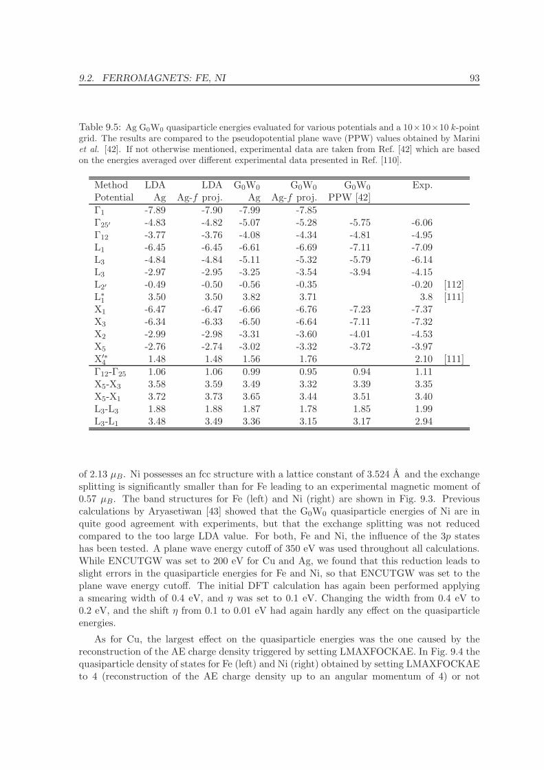
9.2. FERROMAGNETS: FE, NI 93
Table 9.5: Ag G0W0 quasiparticle energies evaluated for various potentials and a 10×10×10 k-pointgrid. The results are compared to the pseudopotential plane wave (PPW) values obtained by Mariniet al. [42]. If not otherwise mentioned, experimental data are taken from Ref. [42] which are basedon the energies averaged over different experimental data presented in Ref. [110].
Method LDA LDA G0W0 G0W0 G0W0 Exp.Potential Ag Ag-f proj. Ag Ag-f proj. PPW [42]
Γ1 -7.89 -7.90 -7.99 -7.85Γ25′ -4.83 -4.82 -5.07 -5.28 -5.75 -6.06Γ12 -3.77 -3.76 -4.08 -4.34 -4.81 -4.95L1 -6.45 -6.45 -6.61 -6.69 -7.11 -7.09L3 -4.84 -4.84 -5.11 -5.32 -5.79 -6.14L3 -2.97 -2.95 -3.25 -3.54 -3.94 -4.15L2′ -0.49 -0.50 -0.56 -0.35 -0.20 [112]L∗
1 3.50 3.50 3.82 3.71 3.8 [111]X1 -6.47 -6.47 -6.66 -6.76 -7.23 -7.37X3 -6.34 -6.33 -6.50 -6.64 -7.11 -7.32X2 -2.99 -2.98 -3.31 -3.60 -4.01 -4.53X5 -2.76 -2.74 -3.02 -3.32 -3.72 -3.97X′∗
4 1.48 1.48 1.56 1.76 2.10 [111]
Γ12-Γ25 1.06 1.06 0.99 0.95 0.94 1.11X5-X3 3.58 3.59 3.49 3.32 3.39 3.35X5-X1 3.72 3.73 3.65 3.44 3.51 3.40L3-L3 1.88 1.88 1.87 1.78 1.85 1.99L3-L1 3.48 3.49 3.36 3.15 3.17 2.94
of 2.13 µB. Ni possesses an fcc structure with a lattice constant of 3.524 A and the exchangesplitting is significantly smaller than for Fe leading to an experimental magnetic moment of0.57 µB. The band structures for Fe (left) and Ni (right) are shown in Fig. 9.3. Previouscalculations by Aryasetiwan [43] showed that the G0W0 quasiparticle energies of Ni are inquite good agreement with experiments, but that the exchange splitting was not reducedcompared to the too large LDA value. For both, Fe and Ni, the influence of the 3p stateshas been tested. A plane wave energy cutoff of 350 eV was used throughout all calculations.While ENCUTGW was set to 200 eV for Cu and Ag, we found that this reduction leads toslight errors in the quasiparticle energies for Fe and Ni, so that ENCUTGW was set to theplane wave energy cutoff. The initial DFT calculation has again been performed applyinga smearing width of 0.4 eV, and η was set to 0.1 eV. Changing the width from 0.4 eV to0.2 eV, and the shift η from 0.1 to 0.01 eV had again hardly any effect on the quasiparticleenergies.
As for Cu, the largest effect on the quasiparticle energies was the one caused by thereconstruction of the AE charge density triggered by setting LMAXFOCKAE. In Fig. 9.4 thequasiparticle density of states for Fe (left) and Ni (right) obtained by setting LMAXFOCKAEto 4 (reconstruction of the AE charge density up to an angular momentum of 4) or not
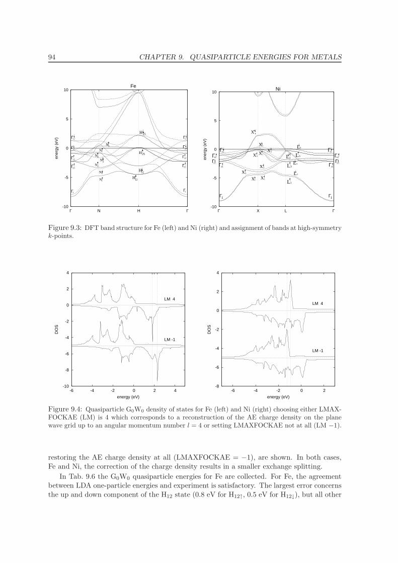
94 CHAPTER 9. QUASIPARTICLE ENERGIES FOR METALS
-10
-5
0
5
10
Γ N H Γ
ener
gy (
eV)
Γ1
Γ25
Γ12
Γ25
Γ12
N1
N1
N2
2N
N1
N4
N3
H12
H12
H25
H25
Γ1
Γ25
Γ12
Γ25
Γ12
Fe
-10
-5
0
5
10
ΓLXΓen
ergy
(eV
)
Γ1
Γ25
Γ25
Γ12
Γ12
X1X 1
X 3
X 3
X 5X 2
X5
X 2
L1
L 1
L3L3
L2L3
L3
Γ1
Γ25
Γ25
Γ12
Γ12
X 4
Ni
Figure 9.3: DFT band structure for Fe (left) and Ni (right) and assignment of bands at high-symmetryk-points.
-10
-8
-6
-4
-2
0
2
4
-6 -4 -2 0 2 4
DO
S
energy (eV)
LM 4
LM -1
-8
-6
-4
-2
0
2
4
-6 -4 -2 0 2
DO
S
energy (eV)
LM 4
LM -1
Figure 9.4: Quasiparticle G0W0 density of states for Fe (left) and Ni (right) choosing either LMAX-FOCKAE (LM) is 4 which corresponds to a reconstruction of the AE charge density on the planewave grid up to an angular momentum number l = 4 or setting LMAXFOCKAE not at all (LM −1).
restoring the AE charge density at all (LMAXFOCKAE = −1), are shown. In both cases,Fe and Ni, the correction of the charge density results in a smaller exchange splitting.
In Tab. 9.6 the G0W0 quasiparticle energies for Fe are collected. For Fe, the agreementbetween LDA one-particle energies and experiment is satisfactory. The largest error concernsthe up and down component of the H12 state (0.8 eV for H12↑, 0.5 eV for H12↓), but all other
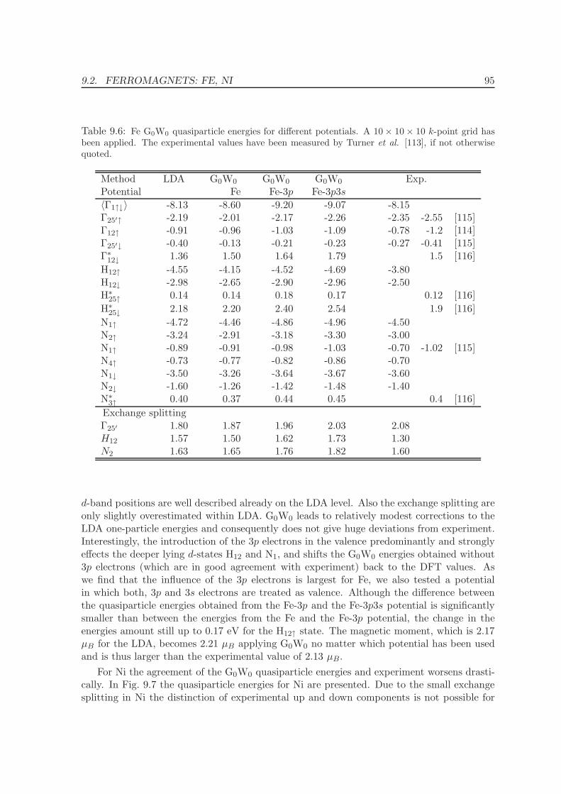
9.2. FERROMAGNETS: FE, NI 95
Table 9.6: Fe G0W0 quasiparticle energies for different potentials. A 10× 10× 10 k-point grid hasbeen applied. The experimental values have been measured by Turner et al. [113], if not otherwisequoted.
Method LDA G0W0 G0W0 G0W0 Exp.Potential Fe Fe-3p Fe-3p3s
〈Γ1↑↓〉 -8.13 -8.60 -9.20 -9.07 -8.15Γ25′↑ -2.19 -2.01 -2.17 -2.26 -2.35 -2.55 [115]Γ12↑ -0.91 -0.96 -1.03 -1.09 -0.78 -1.2 [114]Γ25′↓ -0.40 -0.13 -0.21 -0.23 -0.27 -0.41 [115]Γ∗
12↓ 1.36 1.50 1.64 1.79 1.5 [116]
H12↑ -4.55 -4.15 -4.52 -4.69 -3.80H12↓ -2.98 -2.65 -2.90 -2.96 -2.50H∗
25↑ 0.14 0.14 0.18 0.17 0.12 [116]
H∗25↓ 2.18 2.20 2.40 2.54 1.9 [116]
N1↑ -4.72 -4.46 -4.86 -4.96 -4.50N2↑ -3.24 -2.91 -3.18 -3.30 -3.00N1↑ -0.89 -0.91 -0.98 -1.03 -0.70 -1.02 [115]N4↑ -0.73 -0.77 -0.82 -0.86 -0.70N1↓ -3.50 -3.26 -3.64 -3.67 -3.60N2↓ -1.60 -1.26 -1.42 -1.48 -1.40N∗
3↑ 0.40 0.37 0.44 0.45 0.4 [116]
Exchange splittingΓ25′ 1.80 1.87 1.96 2.03 2.08H12 1.57 1.50 1.62 1.73 1.30N2 1.63 1.65 1.76 1.82 1.60
d-band positions are well described already on the LDA level. Also the exchange splitting areonly slightly overestimated within LDA. G0W0 leads to relatively modest corrections to theLDA one-particle energies and consequently does not give huge deviations from experiment.Interestingly, the introduction of the 3p electrons in the valence predominantly and stronglyeffects the deeper lying d-states H12 and N1, and shifts the G0W0 energies obtained without3p electrons (which are in good agreement with experiment) back to the DFT values. Aswe find that the influence of the 3p electrons is largest for Fe, we also tested a potentialin which both, 3p and 3s electrons are treated as valence. Although the difference betweenthe quasiparticle energies obtained from the Fe-3p and the Fe-3p3s potential is significantlysmaller than between the energies from the Fe and the Fe-3p potential, the change in theenergies amount still up to 0.17 eV for the H12↑ state. The magnetic moment, which is 2.17µB for the LDA, becomes 2.21 µB applying G0W0 no matter which potential has been usedand is thus larger than the experimental value of 2.13 µB.
For Ni the agreement of the G0W0 quasiparticle energies and experiment worsens drasti-cally. In Fig. 9.7 the quasiparticle energies for Ni are presented. Due to the small exchangesplitting in Ni the distinction of experimental up and down components is not possible for
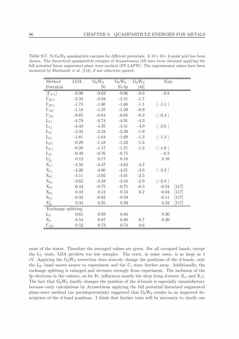
96 CHAPTER 9. QUASIPARTICLE ENERGIES FOR METALS
Table 9.7: Ni G0W0 quasiparticle energies for different potentials. A 10× 10× k-point grid has beenchosen. The theoretical quasiparticle energies of Aryasetiawan [43] have been obtained applying thefull potential linear augmented plane wave method (FP-LAPW). The experimental values have beenmeasured by Eberhardt et al. [118], if not otherwise quoted.
Method LDA G0W0 G0W0 G0W0 Exp.Potential Ni Ni-3p [43]
〈Γ1↑↓〉 -8.99 -9.63 -9.96 -9.0 -8.8Γ25′↑ -2.34 -2.34 -2.41 -1.7Γ25′↓ -1.75 -1.60 -1.66 -1.1 〈 -1.1 〉Γ12↑ -1.18 -1.37 -1.39 -0.9Γ12↓ -0.65 -0.64 -0.65 -0.3 〈 -0.4 〉L1↑ -4.78 -4.74 -4.91 -4.3L1↓ -4.43 -4.35 -4.51 -4.0 〈 -3.6 〉L3↑ -2.33 -2.33 -2.39 -1.9L3↓ -1.81 -1.64 -1.69 -1.3 〈 -1.3 〉L2′↑ -0.29 -1.18 -1.22 -1.3L2′↓ -0.28 -1.17 -1.21 -1.3 〈 -1.0 〉L3↑ -0.49 -0.76 -0.75 −0.2L∗
3↓ 0.12 0.17 0.18 0.16
X1↑ -4.58 -4.47 -4.62 -4.3X1↓ -4.26 -4.06 -4.21 -3.9 〈 -3.3 〉X3↑ -4.11 -3.92 -4.01 -3.5X3↓ -3.62 -3.33 -3.44 -2.9 〈 -2.8 〉X2↑ -0.44 -0.75 -0.75 -0.5 -0.24 [117]X2↓ 0.10 0.12 0.13 0.2 -0.04 [117]X5↑ -0.33 -0.62 -0.59 -0.11 [117]X∗
5↓ 0.34 0.35 0.39 0.22 [117]
Exchange splittingL3 0.61 0.93 0.94 0.36X2 0.54 0.87 0.88 0.7 0.20Γ12↑ 0.52 0.73 0.74 0.6
most of the states. Therefore the averaged values are given. For all occupied bands, exceptthe L2′ state, LDA predicts too low energies. The error, in some cases, is as large as 1eV. Applying the G0W0 correction does scarcely change the positions of the d-bands, onlythe L2′ band moves nearer to experiment and the Γ1 state further away. Additionally, theexchange splitting is enlarged and deviates strongly from experiment. The inclusion of the3p electrons in the valence, as for Fe, influences mostly the deep lying d-states (L1 and X1).The fact that G0W0 hardly changes the position of the d-bands is especially unsatisfactorybecause early calculations by Aryasetiwan applying the full potential linearized augmentedplane-wave method (no pseudopotentials) suggested that G0W0 results in an improved de-scription of the d-band positions. I think that further tests will be necessary to clarify our

9.2. FERROMAGNETS: FE, NI 97
results for Ni.For the ferromagnets Fe and Ni, our G0W0 calculations have lead to relatively small
changes of the LDA one-particle energies. As the LDA description is rather good for Fe andexhibits large errors in the case of Ni, the same holds for the G0W0 results. The inclusion ofthe 3p states in the valence mainly influences the position of the d-bands at low energies. Webelieve that the observed errors in the d-bands for all four considered materials is a resultof the spurious selfinteractions in the GW approximation. This causes an upshift of the dbands for Cu and Ag (0.6 eV error) and pronounced errors for Ni and Fe, where GW predictstoo large band-widths and overestimated the exchange splitting. Only the inclusion of vertexcorrections in Σ (i.e., Σ = iGWΓ) would lift this problem, but such calculations are currentlynot possible.

Part IV
Total energies from ACFDT
99
100
Although the ACFDT formalism was introduced more than 30 years ago [27, 28, 29], andsimilar approaches within many-body perturbation theory (see e.g., [19]) are even older, thecalculation of (RPA)-ACFDT energies has for a long time been restricted to model systemssuch as jellium bulk [132] and jellium slabs and surfaces [29, 119, 120]. The reason for this”delay” is the large computational cost to calculate the response function for an arbitrarysystem. First RPA calculations for molecules have been presented by Furche in 2001 [121].Other RPA calculations for molecules [122, 123, 124, 125, 126, 127] and solids [128, 129, 130]followed shortly afterwards. Although the RPA (setting fxc = 0) accounts for long-rangecorrelation effects such as the van der Waals interaction, molecules have been shown to bestandardly too weakly bonded with a mean absolute error similar to the one found for DFT-PBE. Absolute correlation energies, on the other hand, are throughout too large if the RPAis applied (see e.q., Ref. [35] for the homogenous electron gas). An improvement should beexpected if an appropriate exchange-correlation kernel is introduced for the calculation of theresponse function of the interacting system. Such attempts have, so far, been only applied tomolecular systems [122, 125, 126] [with the exception of the homogenous electron gas (HEG)].In all molecular calculations, fxc was chosen to be independent of the frequency (static- or adiabatic - approximation). An extensive study of atomization energies obtained forexchange-correlation kernels of the form fxc(r, r
′) = δ2Exc/δn(r)δn(r′) derived from differentapproximations to the exchange-correlation energy (LDA, PBE, BP86, B3LYP, PBE0) hasbeen performed in Ref. [126]. The authors found that improvement over the RPA can onlybe obtained if the exchange-correlation kernel is non-local (as it is in the case of B3LYPand PBE0). Similar tests for solids have not been performed so far, but calculations for thehomogenous electron gas [35] suggest that the non-locality of the fxc is important also in thecase of solids.
As the RPA does not fulfill the homogenous electron gas limit a different route to animprovement was supposed by Kurth and Perdew [131]. They included an additional cor-rection term to the RPA correlation energy, ∆Ec, which is introduced in a LDA like way:∆Ec = ELDA
c − ELDA−RPAc , where ELDA
c is the standard LDA correlation energy based onthe exact correlation energy for the homogenous electron gas and ELDA−RPA
c an LDA termbased on the RPA energy of the homogenous electron gas. This method is referred to asRPA+ and results in the correct correlation energy for the HEG per definition. The com-putational cost to calculate the correction term is negligible compared to the RPA energyevaluation. Unfortunately, the RPA+ does not provide an improvement over RPA atomiza-tion energies [121], although Fuchs et al. [122] report that absolute correlation energies areimproved. Lattice constants and bulk moduli are almost the same for RPA and RPA+ [130].
In this part of my thesis I will present results obtained within the ACFDT formalism,which has been introduced in chapter 3. Throughout the present work we will make use of theRPA for the evaluation of the density-density response function of the interacting system. Inchapter 10, we will discuss technical issues concerning the calculation of the RPA correlationenergy in more detail. In chapter 11, RPA energies for molecules (Sec. 11.1), rare gas solids(Sec. 11.2), and extended insulating, semiconducting, and metallic systems (Sec. 11.5) willbe discussed. For the extended systems, besides the lattice constants and bulk moduli, alsothe RPA atomization energies are evaluated. Atomization energies of extended systems have,to the best of our knowledge, not been performed before. This is connected to the difficultyto evaluate atomic energies within a plane wave basis code.
Chapter 10
Implementation of the ACFDTroutines
The total RPA energy is given as a sum of the Hartree-Fock energy evaluated for the KS-DFTwavefunctions (in the following simply referred to as HF energy), and the RPA correlationenergy [see Eq. (3.36)]:
E = Ts[ψKS] + EH [n] +Ex[ψKS] + ERPA
c [ψKS , ǫKS] = EHF [ψKS] + ERPAc .
As we will use the RPA throughout this work, we disregard the index RPA and abreviatethe RPA correlation energy as Ec. The RPA correlation energy Ec is obtained by evaluatingEq. (3.35):
Ec =
∫ ∞
0
dω
2π
∑
q∈BZ
∑
G
(ln[1− χKS(q, iω) ν(q)]
)G,G
+ νG,G(q)χKSG,G(q, iω)
.
Three steps are required for the calculation of the total RPA energy:
(i) Hartree-Fock energy: The Hartree-Fock energy EHF is evaluated for the KS wavefunc-tions determined in a DFT calculation. A high energy cutoff Ecut and dense k-point gridsare required for accurate Hartree-Fock energies. Therefore, the settings for the Hartree-Fockcalculation might differ from the respective values applied in the evaluation of the RPA cor-relation energy.
(ii) Pre-run for RPA correlation energy: For the evaluation of the RPA correlation energy,the KS-DFT wavefunctions and eigenenergies of a large number of unoccupied states arerequired. In this pre-run, all NPW (number of plane wave) solutions of the KS eigenvalueproblem are evaluated by an exact diagonalization of the NPW × NPW Hamilton matrixHG,G′ . The number of plane waves is related to the energy cutoff Ecut by the constraint|G + k|2/2 < Ecut. For a fixed energy cutoff Ecut, the number of plane waves NPW is pro-portional to the volume of the real space cell V , so that this step can become demanding forlarge volumes V . The importance of unoccupied bands also requires special care for the con-struction of the PAW potentials. For the calculation of the RPA correlation energies so calledGW potentials have been constructed that describe scattering properties very accurately up
101
102 CHAPTER 10. IMPLEMENTATION OF THE ACFDT ROUTINES
to ≈ 10 Ry. Furthermore, a d-projector has been introduced for the third row elements,and a f -projector for Ag. These states, while unoccupied, are not too high in energy andtherefore contribute to the response function χKS.
(iii) RPA correlation energy: The response function χKSG,G′(q, iω) is calculated from the wave-
functions and eigenenergies evaluated in the previous step and the RPA correlation energy isdetermined via Eq. (3.35). Some details concerning the evaluation of this expression have al-ready been discussed in Sec. 3.3. What remains to be analyzed is the dependence of the RPAcorrelation energy on the rank of the response function χKS
G,G′ . The sum over reciprocal latticevectors in Eq. (3.35) has to be truncated at some maximal vector Gcut, which is determinedby the relation |G + q|2/2 < Eχ
cut. The dependence of the correlation energy on the energycutoff Eχ
cut will be discussed in Sec. 10.1. Besides the summation over reciprocal lattice vec-tors, the evaluation of the correlation energy requires an integration along the frequency axis.In Sec. 10.2 different frequency integration schemes will be discussed and convergence testswith respect to the number of frequency points will be presented. Sec. 10.3 deals with thecalculation of RPA correlation energies for metals. For metals the long-wavelength (q = 0)response function χ (or more precisely νχ) also contains contributions arising from intrabandtransitions. In Sec. 10.3 several ways will be considered, how to include the intraband termfor the evaluation of the correlation energy.
10.1 Dependence on dimension of the response function
For the calculation of the RPA correlation energy, the dependence on the rank of the responsefunction or the energy cutoff Eχ
cut, respectively, is among the most critical issues. The energycutoff Eχ
cut determines at which point the sum over reciprocal lattice vectors in Eq. (3.35) istruncated, and the convergence of the correlation energy with the maximal considered latticevector turns out to be very slow. This slow convergence is not unique to plane wave basisset codes. If the RPA correlation energy is calculated using a local basis set the highestangular momentum quantum number in the atomic basis set determines the convergence ofthe correlation energy (see Furche [121]).
The calculation of the fully converged correlation energy is not possible, because anincrease in Eχ
cut implies that also the energy cutoff for the plane wave expansion, Ecut, andthe number of bands have to be increased. As a consequence, such calculations will becomeintractable. On the other hand, if an analytic dependence of the correlation energy on Eχ
cut
were known, it would be enough to evaluate the correlation energy for smaller values of Eχcut
and extrapolate the correlation energies according to this dependence. In the following, wewill derive the Eχ
cut dependence of the RPA correlation energy for the homogenous electrongas (HEG). Under the assumption that the ”correlation error” introduced by the neglect ofhigh energy components in the response function behaves similar for the homogenous electrongas and an inhomogeneous system, the determined Eχ
cut dependence can also be applied toany other material.
The correlation energy for the HEG, as for any other system, can be evaluated fromthe difference between the interacting and the independent-particle response function [seeEq. (3.24)], which are coupled by the Dyson equation [Eq. (3.29) if the RPA is applied].With the independent-particle response function of the HEG, the Lindhard function χLind,
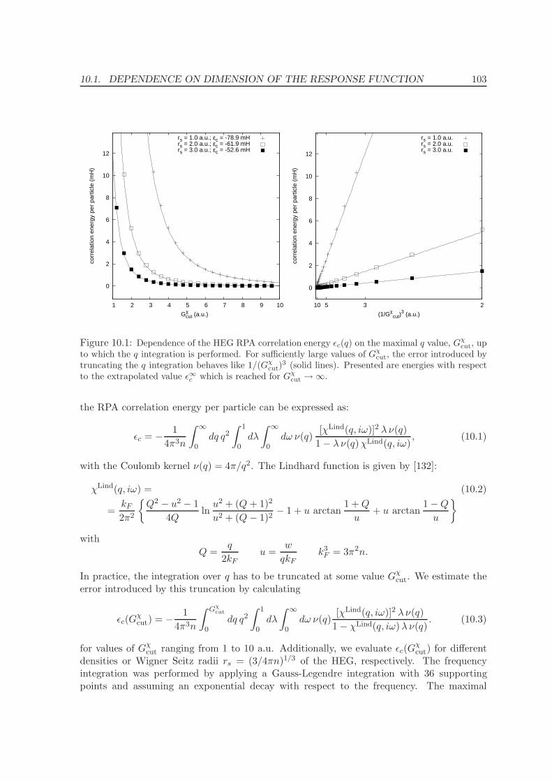
10.1. DEPENDENCE ON DIMENSION OF THE RESPONSE FUNCTION 103
0
2
4
6
8
10
12
1 2 3 4 5 6 7 8 9 10
corr
elat
ion
ener
gy p
er p
artic
le (
mH
)
Gχcut (a.u.)
rs = 1.0 a.u.; εc = -78.9 mHrs = 2.0 a.u.; εc = -61.9 mHrs = 3.0 a.u.; εc = -52.6 mH
0
2
4
6
8
10
12
10 5 3 2
corr
elat
ion
ener
gy p
er p
artic
le (
mH
)
(1/Gχcut)
3 (a.u.)
rs = 1.0 a.u.rs = 2.0 a.u.rs = 3.0 a.u.
Figure 10.1: Dependence of the HEG RPA correlation energy ǫc(q) on the maximal q value, Gχcut, up
to which the q integration is performed. For sufficiently large values of Gχcut, the error introduced by
truncating the q integration behaves like 1/(Gχcut)
3 (solid lines). Presented are energies with respectto the extrapolated value ǫ∞c which is reached for Gχ
cut →∞.
the RPA correlation energy per particle can be expressed as:
ǫc = −1
4π3n
∫ ∞
0dq q2
∫ 1
0dλ
∫ ∞
0dω ν(q)
[χLind(q, iω)]2 λ ν(q)
1− λ ν(q)χLind(q, iω), (10.1)
with the Coulomb kernel ν(q) = 4π/q2. The Lindhard function is given by [132]:
χLind(q, iω) = (10.2)
=kF
2π2
Q2 − u2 − 1
4Qlnu2 + (Q+ 1)2
u2 + (Q− 1)2− 1 + u arctan
1 +Q
u+ u arctan
1−Q
u
with
Q =q
2kFu =
w
qkFk3
F = 3π2n.
In practice, the integration over q has to be truncated at some value Gχcut. We estimate the
error introduced by this truncation by calculating
ǫc(Gχcut) = −
1
4π3n
∫ Gχcut
0dq q2
∫ 1
0dλ
∫ ∞
0dω ν(q)
[χLind(q, iω)]2 λ ν(q)
1− χLind(q, iω)λ ν(q). (10.3)
for values of Gχcut ranging from 1 to 10 a.u. Additionally, we evaluate ǫc(G
χcut) for different
densities or Wigner Seitz radii rs = (3/4πn)1/3 of the HEG, respectively. The frequencyintegration was performed by applying a Gauss-Legendre integration with 36 supportingpoints and assuming an exponential decay with respect to the frequency. The maximal
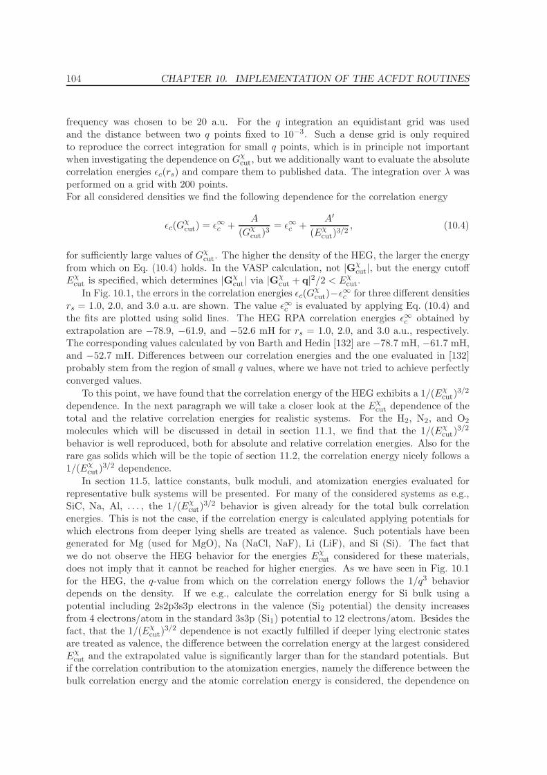
104 CHAPTER 10. IMPLEMENTATION OF THE ACFDT ROUTINES
frequency was chosen to be 20 a.u. For the q integration an equidistant grid was usedand the distance between two q points fixed to 10−3. Such a dense grid is only requiredto reproduce the correct integration for small q points, which is in principle not importantwhen investigating the dependence on Gχ
cut, but we additionally want to evaluate the absolutecorrelation energies ǫc(rs) and compare them to published data. The integration over λ wasperformed on a grid with 200 points.For all considered densities we find the following dependence for the correlation energy
ǫc(Gχcut) = ǫ∞c +
A
(Gχcut)
3= ǫ∞c +
A′
(Eχcut)
3/2, (10.4)
for sufficiently large values of Gχcut. The higher the density of the HEG, the larger the energy
from which on Eq. (10.4) holds. In the VASP calculation, not |Gχcut|, but the energy cutoff
Eχcut is specified, which determines |Gχ
cut| via |Gχcut + q|2/2 < Eχ
cut.
In Fig. 10.1, the errors in the correlation energies ǫc(Gχcut)−ǫ
∞c for three different densities
rs = 1.0, 2.0, and 3.0 a.u. are shown. The value ǫ∞c is evaluated by applying Eq. (10.4) andthe fits are plotted using solid lines. The HEG RPA correlation energies ǫ∞c obtained byextrapolation are −78.9, −61.9, and −52.6 mH for rs = 1.0, 2.0, and 3.0 a.u., respectively.The corresponding values calculated by von Barth and Hedin [132] are −78.7 mH, −61.7 mH,and −52.7 mH. Differences between our correlation energies and the one evaluated in [132]probably stem from the region of small q values, where we have not tried to achieve perfectlyconverged values.
To this point, we have found that the correlation energy of the HEG exhibits a 1/(Eχcut)
3/2
dependence. In the next paragraph we will take a closer look at the Eχcut dependence of the
total and the relative correlation energies for realistic systems. For the H2, N2, and O2
molecules which will be discussed in detail in section 11.1, we find that the 1/(Eχcut)
3/2
behavior is well reproduced, both for absolute and relative correlation energies. Also for therare gas solids which will be the topic of section 11.2, the correlation energy nicely follows a1/(Eχ
cut)3/2 dependence.
In section 11.5, lattice constants, bulk moduli, and atomization energies evaluated forrepresentative bulk systems will be presented. For many of the considered systems as e.g.,SiC, Na, Al, . . . , the 1/(Eχ
cut)3/2 behavior is given already for the total bulk correlation
energies. This is not the case, if the correlation energy is calculated applying potentials forwhich electrons from deeper lying shells are treated as valence. Such potentials have beengenerated for Mg (used for MgO), Na (NaCl, NaF), Li (LiF), and Si (Si). The fact thatwe do not observe the HEG behavior for the energies Eχ
cut considered for these materials,does not imply that it cannot be reached for higher energies. As we have seen in Fig. 10.1for the HEG, the q-value from which on the correlation energy follows the 1/q3 behaviordepends on the density. If we e.g., calculate the correlation energy for Si bulk using apotential including 2s2p3s3p electrons in the valence (Si2 potential) the density increasesfrom 4 electrons/atom in the standard 3s3p (Si1) potential to 12 electrons/atom. Besides thefact, that the 1/(Eχ
cut)3/2 dependence is not exactly fulfilled if deeper lying electronic states
are treated as valence, the difference between the correlation energy at the largest consideredEχ
cut and the extrapolated value is significantly larger than for the standard potentials. Butif the correlation contribution to the atomization energies, namely the difference between thebulk correlation energy and the atomic correlation energy is considered, the dependence on
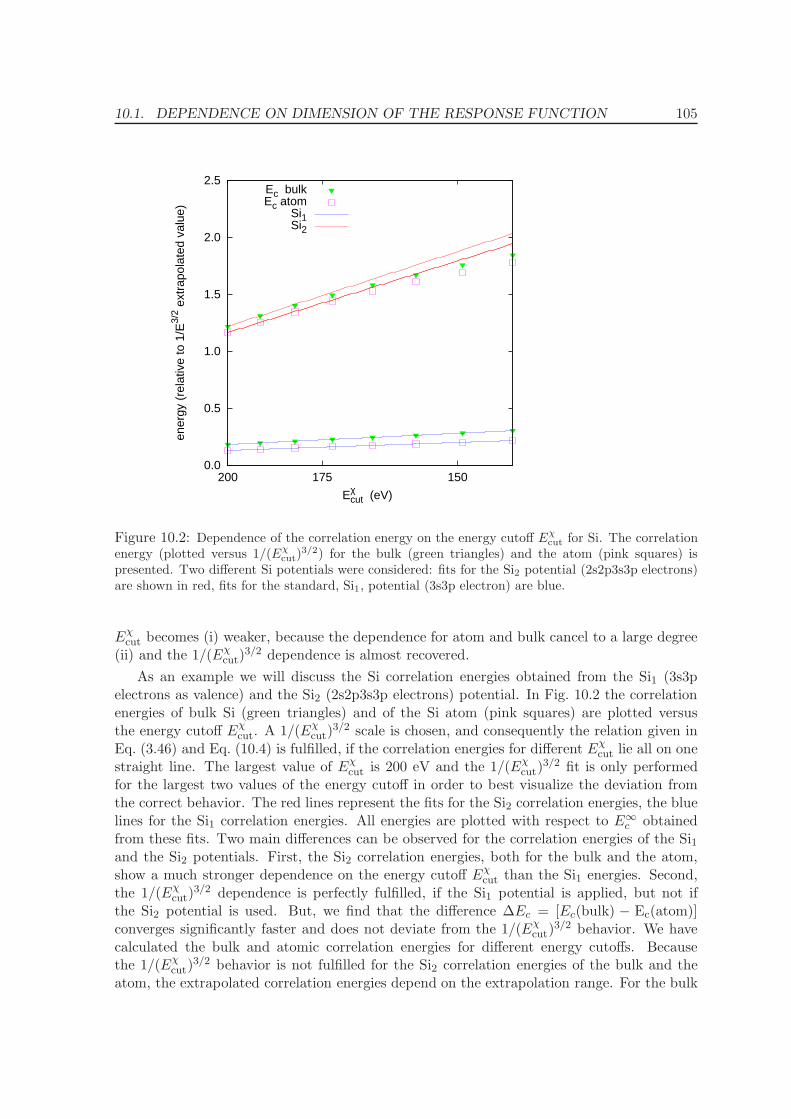
10.1. DEPENDENCE ON DIMENSION OF THE RESPONSE FUNCTION 105
0.0
0.5
1.0
1.5
2.0
2.5
200 175 150
ener
gy (
rela
tive
to 1
/E3/
2 ext
rapo
late
d va
lue)
Eχcut (eV)
Ec bulkEc atom
Si1Si2
Figure 10.2: Dependence of the correlation energy on the energy cutoff Eχcut for Si. The correlation
energy (plotted versus 1/(Eχcut)
3/2) for the bulk (green triangles) and the atom (pink squares) ispresented. Two different Si potentials were considered: fits for the Si2 potential (2s2p3s3p electrons)are shown in red, fits for the standard, Si1, potential (3s3p electron) are blue.
Eχcut becomes (i) weaker, because the dependence for atom and bulk cancel to a large degree
(ii) and the 1/(Eχcut)
3/2 dependence is almost recovered.
As an example we will discuss the Si correlation energies obtained from the Si1 (3s3pelectrons as valence) and the Si2 (2s2p3s3p electrons) potential. In Fig. 10.2 the correlationenergies of bulk Si (green triangles) and of the Si atom (pink squares) are plotted versusthe energy cutoff Eχ
cut. A 1/(Eχcut)
3/2 scale is chosen, and consequently the relation given inEq. (3.46) and Eq. (10.4) is fulfilled, if the correlation energies for different Eχ
cut lie all on onestraight line. The largest value of Eχ
cut is 200 eV and the 1/(Eχcut)
3/2 fit is only performedfor the largest two values of the energy cutoff in order to best visualize the deviation fromthe correct behavior. The red lines represent the fits for the Si2 correlation energies, the bluelines for the Si1 correlation energies. All energies are plotted with respect to E∞
c obtainedfrom these fits. Two main differences can be observed for the correlation energies of the Si1and the Si2 potentials. First, the Si2 correlation energies, both for the bulk and the atom,show a much stronger dependence on the energy cutoff Eχ
cut than the Si1 energies. Second,the 1/(Eχ
cut)3/2 dependence is perfectly fulfilled, if the Si1 potential is applied, but not if
the Si2 potential is used. But, we find that the difference ∆Ec = [Ec(bulk) − Ec(atom)]converges significantly faster and does not deviate from the 1/(Eχ
cut)3/2 behavior. We have
calculated the bulk and atomic correlation energies for different energy cutoffs. Becausethe 1/(Eχ
cut)3/2 behavior is not fulfilled for the Si2 correlation energies of the bulk and the
atom, the extrapolated correlation energies depend on the extrapolation range. For the bulk
106 CHAPTER 10. IMPLEMENTATION OF THE ACFDT ROUTINES
correlation energy we find an extrapolated correlation energy of −17.437 eV for the Eχcut
range [140,200] eV, −19.016 eV for [215,300] eV, and −19.386 eV for [250,350] eV. Butbecause the extrapolated correlation energies of both the bulk and the atom show a verysimilar dependence on the extrapolation range, the difference ∆Ec is −1.522 eV for [140,200]eV, −1.509 eV for [215,300] eV, and −1.508 eV [250,350] eV, and it is therefore possibleto obtained well converged atomization energies even if the individual contributions to theenergy are not completely converged.
For the lattice constant and bulk moduli determined in section 11.5, we find that valueswith and without 1/(Eχ
cut)3/2 extrapolation can differ significantly (by up to 1.5% in the
volume), whereas the dependence on the specific interpolation range is small, also for systemswhere the 1/(Eχ
cut)3/2 dependence is not strictly fulfilled.
In the latest VASP version the correlation energy is standardly evaluated for 8 cutoffenergies Eχ
cut starting with the value of ENCUTGW set in the INCAR file and decreasing insteps of 5 % of ENCUTGW. The extrapolated correlation energy is written to the OUTCARfile together with the correlation energies at the single values of Eχ
cut.
10.2 Frequency integration
We calculate the correlation energy from the linear response function at imaginary frequen-cies. The response function χ(iω) is a smooth function of the frequency and the frequencyintegration therefore does not constitute a fundamental problem. As the number of fre-quency points enters the computational time linearly, an optimal choice for the frequencygrid is nevertheless desirable.
All integration schemes presented in the following are based on a Gauss-Legendre inte-gration. The weights and supporting points for a Gauss-Legendre integration in the interval[0,1] are tabulated in VASP for up to 64 supporting points. According to the Gauss-Legendreintegration scheme, the integral of a polynomial of degree 2N − 1 is exactly determined by aN -point sum
∫ 1
0f(x) dx =
N∑
i
wi f(xi), (10.5)
where wi and xi are the Gauss-Legendre weights and supporting points, respectively. Forthe frequency integration as present in the evaluation of the correlation energy, an integralof the type
Ec =
∫ ∞
0g(ω) dω (10.6)
has to be calculated. The integrand g(ω) = ln(1 − νχ) + νχ exhibits an exponential decayover a wide range of frequencies1. In order to make use of Eq. (10.5), a weighting function
1If only one single transitions contributes to the response function χ(iω), the frequency dependence of theresponse function is proportional to ∆ǫ/(∆ǫ2 + ω2), ∆ǫ being the energy difference between the contributingstates [consider Eq. (2.35) for imaginary frequencies]. For large frequencies, the correlation energy thus decays∝ 1/ω4. Nevertheless, fast convergence is found by assuming an exponential decay.
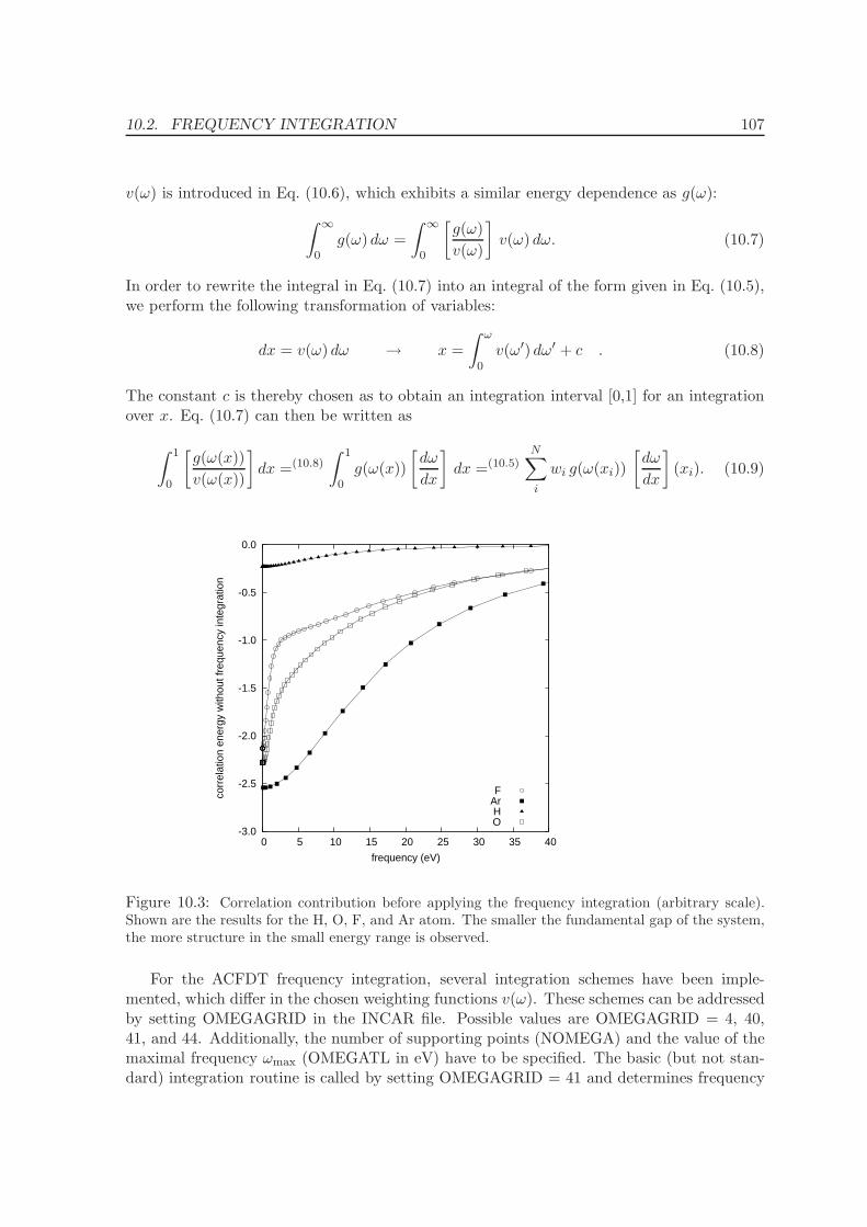
10.2. FREQUENCY INTEGRATION 107
v(ω) is introduced in Eq. (10.6), which exhibits a similar energy dependence as g(ω):
∫ ∞
0g(ω) dω =
∫ ∞
0
[g(ω)
v(ω)
]v(ω) dω. (10.7)
In order to rewrite the integral in Eq. (10.7) into an integral of the form given in Eq. (10.5),we perform the following transformation of variables:
dx = v(ω) dω → x =
∫ ω
0v(ω′) dω′ + c . (10.8)
The constant c is thereby chosen as to obtain an integration interval [0,1] for an integrationover x. Eq. (10.7) can then be written as
∫ 1
0
[g(ω(x))
v(ω(x))
]dx =(10.8)
∫ 1
0g(ω(x))
[dω
dx
]dx =(10.5)
N∑
i
wi g(ω(xi))
[dω
dx
](xi). (10.9)
-3.0
-2.5
-2.0
-1.5
-1.0
-0.5
0.0
0 5 10 15 20 25 30 35 40
corr
elat
ion
ener
gy w
ithou
t fre
quen
cy in
tegr
atio
n
frequency (eV)
FArHO
Figure 10.3: Correlation contribution before applying the frequency integration (arbitrary scale).Shown are the results for the H, O, F, and Ar atom. The smaller the fundamental gap of the system,the more structure in the small energy range is observed.
For the ACFDT frequency integration, several integration schemes have been imple-mented, which differ in the chosen weighting functions v(ω). These schemes can be addressedby setting OMEGAGRID in the INCAR file. Possible values are OMEGAGRID = 4, 40,41, and 44. Additionally, the number of supporting points (NOMEGA) and the value of themaximal frequency ωmax (OMEGATL in eV) have to be specified. The basic (but not stan-dard) integration routine is called by setting OMEGAGRID = 41 and determines frequency
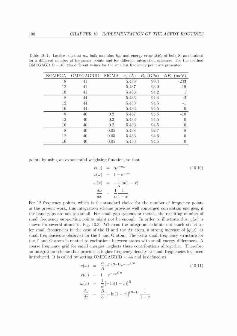
108 CHAPTER 10. IMPLEMENTATION OF THE ACFDT ROUTINES
Table 10.1: Lattice constant a0, bulk modulus B0, and energy error ∆E0 of bulk Si as obtainedfor a different number of frequency points and for different integration schemes. For the methodOMEGAGRID = 40, two different values for the smallest frequency point are presented.
NOMEGA OMEGAGRID SIGMA a0 (A) B0 (GPa) ∆E0 (meV)
8 41 5.438 99.4 -23312 41 5.437 93.0 -1916 41 5.433 94.2 1
8 44 5.433 94.4 -212 44 5.433 94.5 -116 44 5.433 94.5 0
8 40 0.2 5.437 93.6 -1012 40 0.2 5.433 94.5 016 40 0.2 5.433 94.5 0
8 40 0.05 5.438 92.7 812 40 0.05 5.433 94.6 016 40 0.05 5.433 94.5 0
points by using an exponential weighting function, so that
v(ω) = αe−αω (10.10)
x(ω) = 1− e−αω
ω(x) = −1
αln(1− x)
dω
dx=
1
α
1
1− x.
For 12 frequency points, which is the standard choice for the number of frequency pointsin the present work, this integration scheme provides well converged correlation energies, ifthe band gaps are not too small. For small gap systems or metals, the resulting number ofsmall frequency supporting points might not be enough. In order to illustrate this, g(ω) isshown for several atoms in Fig. 10.3. Whereas the integrand exhibits not much structurefor small frequencies in the case of the H and the Ar atom, a strong increase of |g(ω)| atsmall frequencies is observed for the F and O atom. The extra small frequency structure forthe F and O atom is related to excitations between states with small energy differences. Acoarse frequency grid for small energies neglects these contributions alltogether. Thereforean integration scheme that provides a higher frequency density at small frequencies has beenintroduced. It is called by setting OMEGAGRID = 44 and is defined as
v(ω) =α
Bω(1/B−1)e−αω1/B
(10.11)
x(ω) = 1− e−αω1/B
ω(x) =1
α[− ln(1− x)]B
dω
dx=
B
α[− ln(1− x)](B−1) 1
1− x.
10.3. K-POINT CONVERGENCE AND Γ-POINT CORRECTION FOR METALS 109
Finally, a third kind of integration scheme was introduced, which guarantees a denser fre-quency grid at smaller frequencies than provided by OMEGAGRID = 41, but yields a similarbehavior for large frequencies. By choosing OMEGAGRID = 4 or 40, the frequency pointsare determined according to
ω(x) = −1
αln[(1− b)(1 − x) + b(1− x)2
](10.12)
dω
dx=
1
α
(1− b) + 2 b (1 − x)
(1− b) (1− x) + b (1− x)2. (10.13)
This integration scheme occurs in two flavors. For OMEGAGRID = 4, which is the standardsetting for ACFDT calculations, a fixed value is chosen for b, for OMEGAGRID = 40, thesmallest frequency is set to the value of SIGMA provided in the INCAR file2. Numeroustests have confirmed that OMEGAGRID = 4 or OMEGAGRID = 40 provide a very goodcompromise between the number of frequency points and the accuracy of the frequencyintegration.
One of the systems for which the convergence with the number of frequency points isespecially slow is bulk Si. In table 10.1 the Si equilibrium lattice constant a0, the bulkmodulus B0, and the energy error ∆E0 obtained from different integration schemes anddifferent number of frequency points are summarized. A 4×4×4 k-point grid has been used.For all, but the simple exponential Gauss-Legendre integration (OMEGAGRID = 41), 12frequency points provide well converged lattice constants, bulk moduli and total energies.
10.3 k-point convergence and Γ-point correction for metals
Although metals do not represent a fundamental problem for (RPA-)ACFDT calculations,they require more attention with respect to the k-point convergence than semiconductorsand insulators. In fact, already the sampling of the metallic Fermi surface in standard DFTcalculations requires a denser k-point grid. Here the k-point grid affects the precision intwo ways, first because χ(q) is only evaluated using a finite set of k-points, second becauseχ(q) is only summed over a finite grid of q-points. These two grids, the k-point grid usedin the calculation of χ(q) and the q-point grid used in the final evaluation of the correlationenergy, are independent from each other, but they will be chosen identical throughout thiswork. A second difficulty arises for metals from the existence of intraband transitions withinone partially-filled band crossing the Fermi level. These contributions to χ(q) ν(q) are rou-tinely calculated for q 6= 0 , but for the long-wavelength limit q → 0, a direct evaluation ofthese terms leads to an indefinite expression (see Sec. 2.8). This indefiniteness in the long-wavelength intraband term of νχ can however be lifted and the intraband contributions (orDrude term) can be expressed via the plasma frequency ω [see Eq. (2.106)]. In the following,we will discuss the influence of the Drude term on the correlation energy for the example ofthe homogenous electron gas (HEG) and present different ways how to include the intrabandlong-wavelength contribution.
2If ISMEAR is set ≥ 0 in the INCAR, the one-electron levels are broadened or smeared. The parameterSIGMA controls the width of the broadening function. It is reasonable to expect that the user will chosevalues corresponding roughly to the smallest excitation energies in the system under consideration.
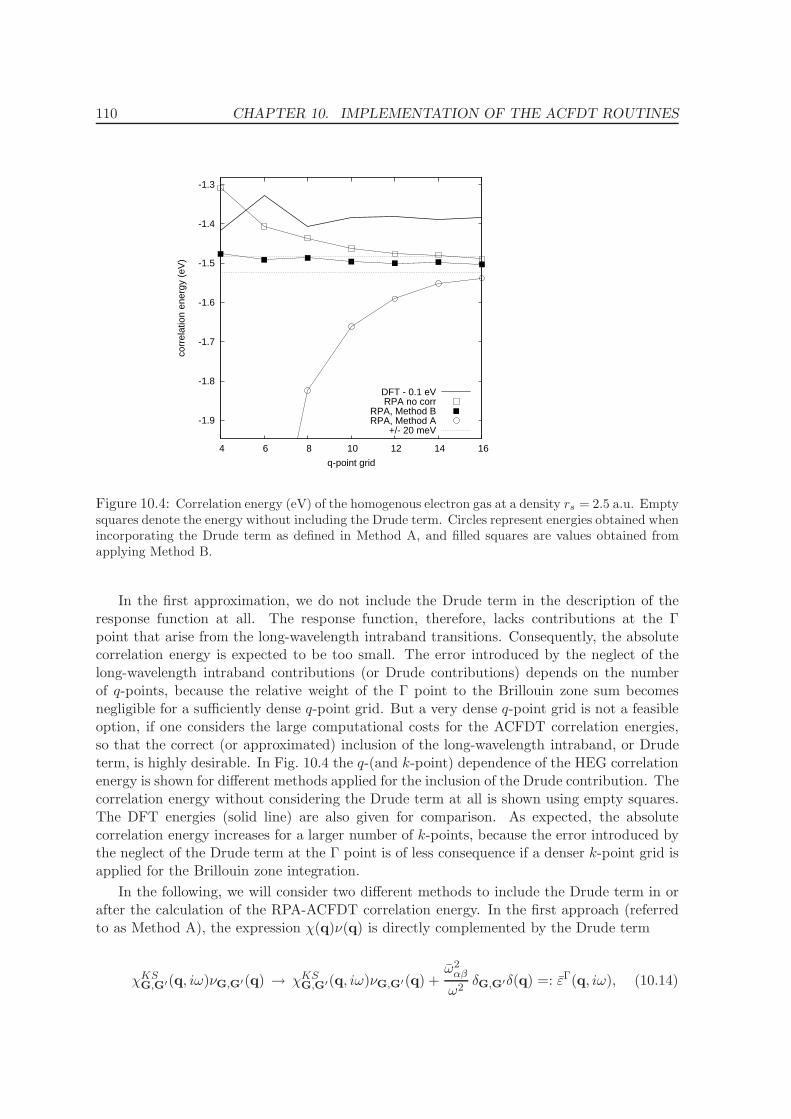
110 CHAPTER 10. IMPLEMENTATION OF THE ACFDT ROUTINES
-1.9
-1.8
-1.7
-1.6
-1.5
-1.4
-1.3
4 6 8 10 12 14 16
corr
elat
ion
ener
gy (
eV)
q-point grid
DFT - 0.1 eVRPA no corr
RPA, Method BRPA, Method A
+/- 20 meV
Figure 10.4: Correlation energy (eV) of the homogenous electron gas at a density rs = 2.5 a.u. Emptysquares denote the energy without including the Drude term. Circles represent energies obtained whenincorporating the Drude term as defined in Method A, and filled squares are values obtained fromapplying Method B.
In the first approximation, we do not include the Drude term in the description of theresponse function at all. The response function, therefore, lacks contributions at the Γpoint that arise from the long-wavelength intraband transitions. Consequently, the absolutecorrelation energy is expected to be too small. The error introduced by the neglect of thelong-wavelength intraband contributions (or Drude contributions) depends on the numberof q-points, because the relative weight of the Γ point to the Brillouin zone sum becomesnegligible for a sufficiently dense q-point grid. But a very dense q-point grid is not a feasibleoption, if one considers the large computational costs for the ACFDT correlation energies,so that the correct (or approximated) inclusion of the long-wavelength intraband, or Drudeterm, is highly desirable. In Fig. 10.4 the q-(and k-point) dependence of the HEG correlationenergy is shown for different methods applied for the inclusion of the Drude contribution. Thecorrelation energy without considering the Drude term at all is shown using empty squares.The DFT energies (solid line) are also given for comparison. As expected, the absolutecorrelation energy increases for a larger number of k-points, because the error introduced bythe neglect of the Drude term at the Γ point is of less consequence if a denser k-point grid isapplied for the Brillouin zone integration.
In the following, we will consider two different methods to include the Drude term in orafter the calculation of the RPA-ACFDT correlation energy. In the first approach (referredto as Method A), the expression χ(q)ν(q) is directly complemented by the Drude term
χKSG,G′(q, iω)νG,G′(q) → χKS
G,G′(q, iω)νG,G′(q) +ω2
αβ
ω2δG,G′δ(q) =: εΓ(q, iω), (10.14)
10.3. K-POINT CONVERGENCE AND Γ-POINT CORRECTION FOR METALS 111
where the plasma frequency tensor is given by Eq. (2.106). If we performed a q-integrationover the Brillouin zone, Eq. (10.14) would result in an exact expression for the correlationenergy. But as we approximate the Brillouin zone integration as a sum over discrete q-points and since we consequently replace the integral over the Γ-centered volume V (Γ) bythe integrand evaluated at the Γ-point times V (Γ), i.e.,
V
(2π)3
∫
V (Γ)
d3q ln[1− εΓ(q, iω)
]+ εΓ(q, iω) →
V
(2π)3V (Γ) ln
[1− εΓ(0, iω)
]+ εΓ(0, iω), (10.15)
method A strongly overestimates the contribution caused by the Drude term. The absolutecorrelation energies evaluated applying method A will therefore be too large, especially for acoarse q-point grid which results in large volumes V (Γ). This can be also seen from Fig. 10.4,where correlation energies obtained from Method A are given by empty circles.
A second, denser q′-point grid could be introduced around the Γ point in order to allowa better numerical integration for small values of q. But this would still require an increasednumber of χKS
G,G′(q, iω) νG,G′(q) evaluations. We proceed along this line, but replace the
KS response function χKS of the considered system by the independent-particle responsefunction of the HEG, the Lindhard function χLind(q) [see Eq. (10.2)]. The density of theHEG, n∗, is thereby chosen as to obey the free electron relation for the plasma frequencycalculated for the respective system (Method B):
ω2 =4πe2n∗h2
m. (10.16)
For metals with high, cubic symmetry, this is well defined since ω := ωxx = ωyy = ωzz. Forlow symmetry systems, one could consider the density corresponding to ω2 = Tr[ω2
α,β]/3.
The evaluation of the respective correlation correction EΓc
EΓc =
V
(2π)3
∫
V (Γ)
d3q
∫ ∞
0dωln[1− χLind(q, iω; ω)ν(q)
]+ χLind(q, iω; ω)ν(q)
(10.17)
can be performed numerically and independently of the actual RPA calculations. The cor-rection calculated from Eq. (10.17) is then simply added to the RPA correlation energyobtained without inclusion of the Drude term. More technical details about the integrationof Eq. (10.17) will be discussed in the next subsection. In Fig. 10.4 the correlation energiescalculated from Method B are shown using black squares. The convergence with respect tothe number of q-points is now significantly improved compared to the correlation energieswithout considering the Drude term (empty squares).
10.3.1 Γ-point corrections: Technical details
The Γ-point correction EΓc is evaluated by summing over
EΓc (qi) :=
∫ ∞
0dωln[1− χLind(qi, iω; ω) ν(qi)
]+ χLind(qi, iω; ω) ν(qi)
(10.18)
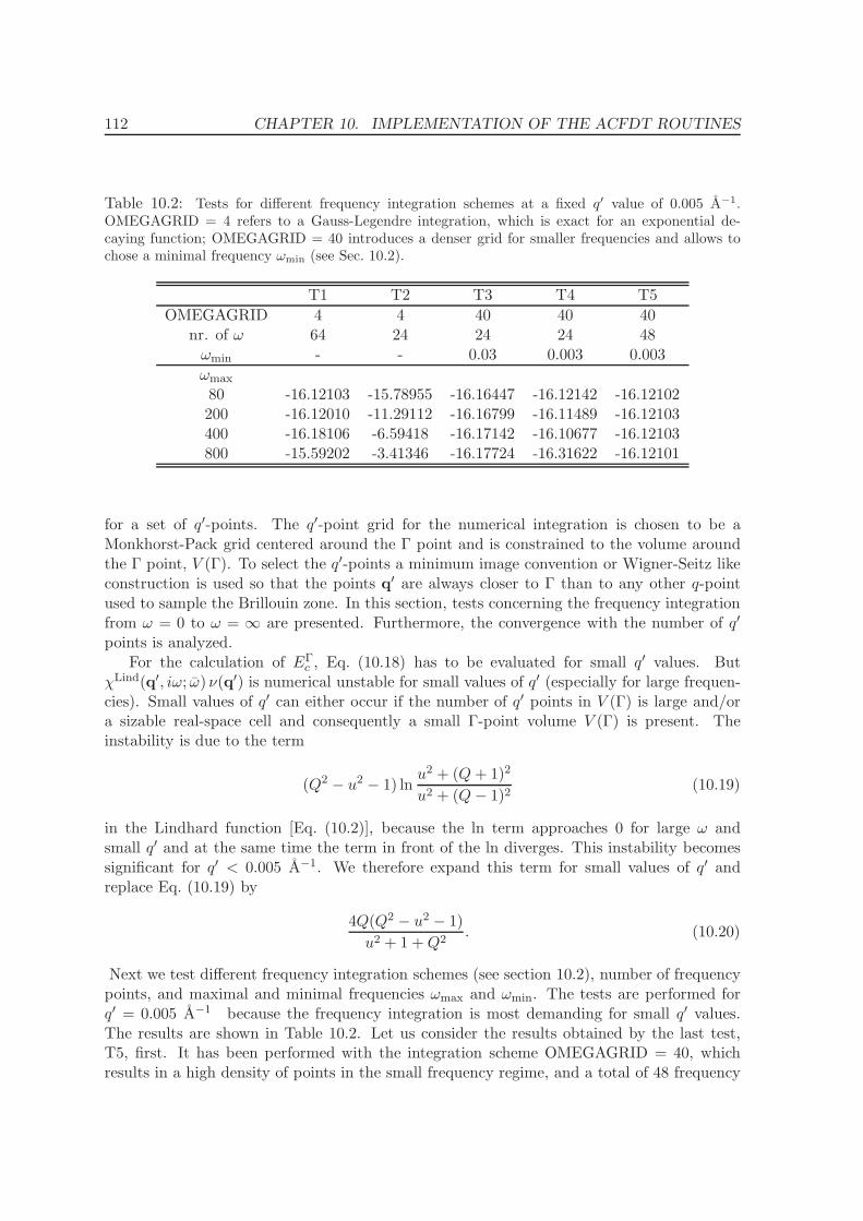
112 CHAPTER 10. IMPLEMENTATION OF THE ACFDT ROUTINES
Table 10.2: Tests for different frequency integration schemes at a fixed q′ value of 0.005 A−1.OMEGAGRID = 4 refers to a Gauss-Legendre integration, which is exact for an exponential de-caying function; OMEGAGRID = 40 introduces a denser grid for smaller frequencies and allows tochose a minimal frequency ωmin (see Sec. 10.2).
T1 T2 T3 T4 T5
OMEGAGRID 4 4 40 40 40nr. of ω 64 24 24 24 48ωmin - - 0.03 0.003 0.003
ωmax
80 -16.12103 -15.78955 -16.16447 -16.12142 -16.12102200 -16.12010 -11.29112 -16.16799 -16.11489 -16.12103400 -16.18106 -6.59418 -16.17142 -16.10677 -16.12103800 -15.59202 -3.41346 -16.17724 -16.31622 -16.12101
for a set of q′-points. The q′-point grid for the numerical integration is chosen to be aMonkhorst-Pack grid centered around the Γ point and is constrained to the volume aroundthe Γ point, V (Γ). To select the q′-points a minimum image convention or Wigner-Seitz likeconstruction is used so that the points q′ are always closer to Γ than to any other q-pointused to sample the Brillouin zone. In this section, tests concerning the frequency integrationfrom ω = 0 to ω = ∞ are presented. Furthermore, the convergence with the number of q′
points is analyzed.For the calculation of EΓ
c , Eq. (10.18) has to be evaluated for small q′ values. ButχLind(q′, iω; ω) ν(q′) is numerical unstable for small values of q′ (especially for large frequen-cies). Small values of q′ can either occur if the number of q′ points in V (Γ) is large and/ora sizable real-space cell and consequently a small Γ-point volume V (Γ) is present. Theinstability is due to the term
(Q2 − u2 − 1) lnu2 + (Q+ 1)2
u2 + (Q− 1)2(10.19)
in the Lindhard function [Eq. (10.2)], because the ln term approaches 0 for large ω andsmall q′ and at the same time the term in front of the ln diverges. This instability becomessignificant for q′ < 0.005 A−1. We therefore expand this term for small values of q′ andreplace Eq. (10.19) by
4Q(Q2 − u2 − 1)
u2 + 1 +Q2. (10.20)
Next we test different frequency integration schemes (see section 10.2), number of frequencypoints, and maximal and minimal frequencies ωmax and ωmin. The tests are performed forq′ = 0.005 A−1 because the frequency integration is most demanding for small q′ values.The results are shown in Table 10.2. Let us consider the results obtained by the last test,T5, first. It has been performed with the integration scheme OMEGAGRID = 40, whichresults in a high density of points in the small frequency regime, and a total of 48 frequency
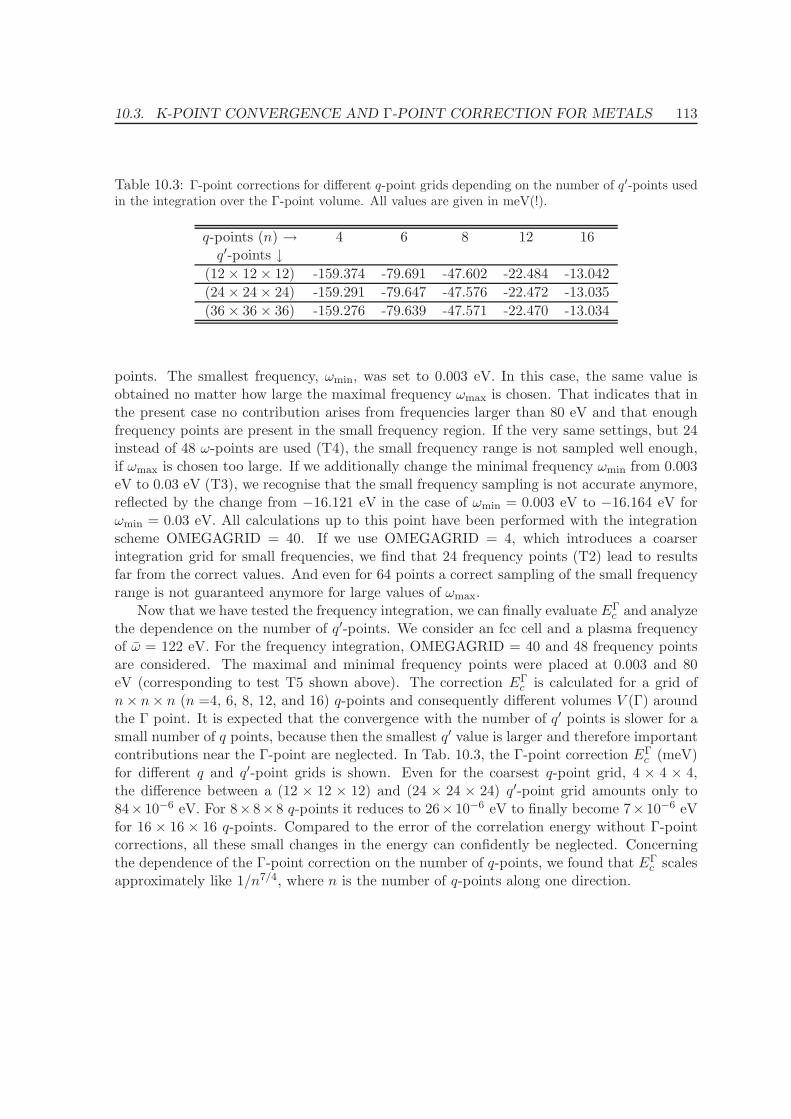
10.3. K-POINT CONVERGENCE AND Γ-POINT CORRECTION FOR METALS 113
Table 10.3: Γ-point corrections for different q-point grids depending on the number of q′-points usedin the integration over the Γ-point volume. All values are given in meV(!).
q-points (n) → 4 6 8 12 16q′-points ↓
(12× 12× 12) -159.374 -79.691 -47.602 -22.484 -13.042
(24× 24× 24) -159.291 -79.647 -47.576 -22.472 -13.035
(36× 36× 36) -159.276 -79.639 -47.571 -22.470 -13.034
points. The smallest frequency, ωmin, was set to 0.003 eV. In this case, the same value isobtained no matter how large the maximal frequency ωmax is chosen. That indicates that inthe present case no contribution arises from frequencies larger than 80 eV and that enoughfrequency points are present in the small frequency region. If the very same settings, but 24instead of 48 ω-points are used (T4), the small frequency range is not sampled well enough,if ωmax is chosen too large. If we additionally change the minimal frequency ωmin from 0.003eV to 0.03 eV (T3), we recognise that the small frequency sampling is not accurate anymore,reflected by the change from −16.121 eV in the case of ωmin = 0.003 eV to −16.164 eV forωmin = 0.03 eV. All calculations up to this point have been performed with the integrationscheme OMEGAGRID = 40. If we use OMEGAGRID = 4, which introduces a coarserintegration grid for small frequencies, we find that 24 frequency points (T2) lead to resultsfar from the correct values. And even for 64 points a correct sampling of the small frequencyrange is not guaranteed anymore for large values of ωmax.
Now that we have tested the frequency integration, we can finally evaluate EΓc and analyze
the dependence on the number of q′-points. We consider an fcc cell and a plasma frequencyof ω = 122 eV. For the frequency integration, OMEGAGRID = 40 and 48 frequency pointsare considered. The maximal and minimal frequency points were placed at 0.003 and 80eV (corresponding to test T5 shown above). The correction EΓ
c is calculated for a grid ofn× n× n (n =4, 6, 8, 12, and 16) q-points and consequently different volumes V (Γ) aroundthe Γ point. It is expected that the convergence with the number of q′ points is slower for asmall number of q points, because then the smallest q′ value is larger and therefore importantcontributions near the Γ-point are neglected. In Tab. 10.3, the Γ-point correction EΓ
c (meV)for different q and q′-point grids is shown. Even for the coarsest q-point grid, 4 × 4 × 4,the difference between a (12 × 12 × 12) and (24 × 24 × 24) q′-point grid amounts only to84× 10−6 eV. For 8× 8× 8 q-points it reduces to 26× 10−6 eV to finally become 7× 10⁻⁶ eVfor 16 × 16 × 16 q-points. Compared to the error of the correlation energy without Γ-pointcorrections, all these small changes in the energy can confidently be neglected. Concerningthe dependence of the Γ-point correction on the number of q-points, we found that EΓ
c scalesapproximately like 1/n7/4, where n is the number of q-points along one direction.
Chapter 11
Application of the ACFDT
11.1 Molecules - H2, O2, N2
The following calculations of the H2, O2, and N2 atomization energies provide a test for ourimplementation of the RPA-ACFDT routines. Our results will be compared to the ones ob-tained by Furche [121] using a local basis set code. His RPA routines have been implementedin the Møller-Plesset (MP2) module MPGRAD [133] of the program TURBOMOLE [134]and a cc-pVXZ (correlation consistent polarized valence electron X zeta) basis set was ap-plied. Similar to the slow convergence of our correlation energies with the maximal reciprocallattice vector determined by Eχ
cut (see section 10.1), Furche’s correlation energies exhibit a
ERPAc (X) = ERPA
c (∞) +A/X3 (11.1)
dependence on the maximal angular momentum X used for the construction of the basis set.If we compare to his correlation energies, we always refer to his extrapolated values.
For a test set of 12 molecules including e.g., results for HF, CO, CO2, H2O, Furchefound that the RPA leads to a general underestimation of the atomization energy ∆E =∑E(atom) − E(mol). The RPA atomization energies for H2, N2, O2, F2, and Si2 (errors
smaller than 9 kcal/mol ≈ 0.4 eV) are improved compared to the DFT-PBE results. Forthe other molecules, PBE atomization energies are closer to experiment. The Hartree-Fockatomization energies ∆EHF =
∑EHF (atom) − EHF (mol) are in all cases much too small,
deviating from the experimental energies by 25 kcal/mol1≈ 1.1 eV for H2, 117 kcal/mol ≈5.1 eV for N2, and 155 kcal/mol ≈ 6.7 eV for CO2.
In the present work, we focus on the atomization energies for H2, O2, and N2. The bondlength is fixed to the experimental value (0.7413 A for H2, 1.208 A for O2, and 1.098 Afor N2). The generalized gradient approximation by Perdew, Burke, and Ernzerhof (PBE)[12] was used for the representation of the exchange-correlation energy in the calculation ofthe KS-DFT eigenenergies and wavefunctions. In order to achieve very accurate results foroxygen and nitrogen, we applied different potentials for the evaluation of the HF energy, EHF ,and the RPA correlation energy, Ec. For the calculation of the Hartree-Fock energy, EHF ,potentials with small core-radii have been considered. For the RPA correlation energy, whereunoccupied states have to be correctly represented, GW potentials that describe scattering
11 kcal/mol = 43.364 meV
114
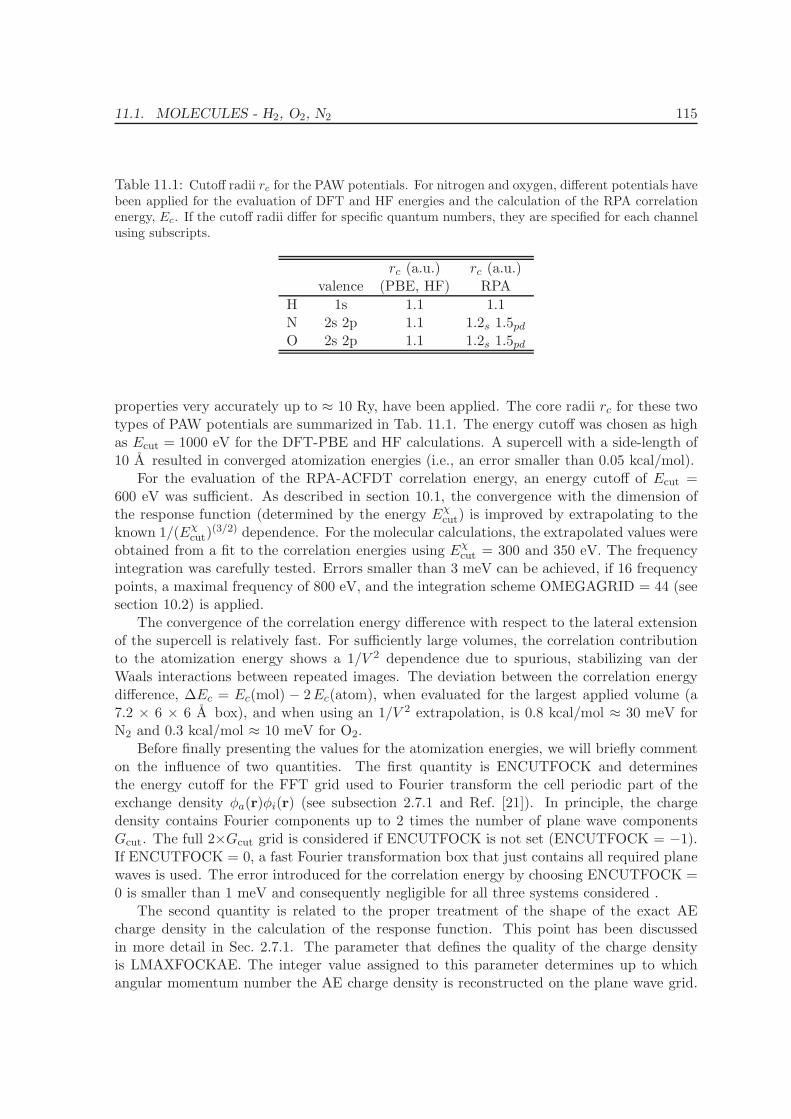
11.1. MOLECULES - H2, O2, N2 115
Table 11.1: Cutoff radii rc for the PAW potentials. For nitrogen and oxygen, different potentials havebeen applied for the evaluation of DFT and HF energies and the calculation of the RPA correlationenergy, Ec. If the cutoff radii differ for specific quantum numbers, they are specified for each channelusing subscripts.
rc (a.u.) rc (a.u.)valence (PBE, HF) RPA
H 1s 1.1 1.1N 2s 2p 1.1 1.2s 1.5pd
O 2s 2p 1.1 1.2s 1.5pd
properties very accurately up to ≈ 10 Ry, have been applied. The core radii rc for these twotypes of PAW potentials are summarized in Tab. 11.1. The energy cutoff was chosen as highas Ecut = 1000 eV for the DFT-PBE and HF calculations. A supercell with a side-length of10 A resulted in converged atomization energies (i.e., an error smaller than 0.05 kcal/mol).
For the evaluation of the RPA-ACFDT correlation energy, an energy cutoff of Ecut =600 eV was sufficient. As described in section 10.1, the convergence with the dimension ofthe response function (determined by the energy Eχ
cut) is improved by extrapolating to theknown 1/(Eχ
cut)(3/2) dependence. For the molecular calculations, the extrapolated values were
obtained from a fit to the correlation energies using Eχcut = 300 and 350 eV. The frequency
integration was carefully tested. Errors smaller than 3 meV can be achieved, if 16 frequencypoints, a maximal frequency of 800 eV, and the integration scheme OMEGAGRID = 44 (seesection 10.2) is applied.
The convergence of the correlation energy difference with respect to the lateral extensionof the supercell is relatively fast. For sufficiently large volumes, the correlation contributionto the atomization energy shows a 1/V 2 dependence due to spurious, stabilizing van derWaals interactions between repeated images. The deviation between the correlation energydifference, ∆Ec = Ec(mol) − 2Ec(atom), when evaluated for the largest applied volume (a7.2 × 6 × 6 A box), and when using an 1/V 2 extrapolation, is 0.8 kcal/mol ≈ 30 meV forN2 and 0.3 kcal/mol ≈ 10 meV for O2.
Before finally presenting the values for the atomization energies, we will briefly commenton the influence of two quantities. The first quantity is ENCUTFOCK and determinesthe energy cutoff for the FFT grid used to Fourier transform the cell periodic part of theexchange density φa(r)φi(r) (see subsection 2.7.1 and Ref. [21]). In principle, the chargedensity contains Fourier components up to 2 times the number of plane wave componentsGcut. The full 2×Gcut grid is considered if ENCUTFOCK is not set (ENCUTFOCK = −1).If ENCUTFOCK = 0, a fast Fourier transformation box that just contains all required planewaves is used. The error introduced for the correlation energy by choosing ENCUTFOCK =0 is smaller than 1 meV and consequently negligible for all three systems considered .
The second quantity is related to the proper treatment of the shape of the exact AEcharge density in the calculation of the response function. This point has been discussedin more detail in Sec. 2.7.1. The parameter that defines the quality of the charge densityis LMAXFOCKAE. The integer value assigned to this parameter determines up to whichangular momentum number the AE charge density is reconstructed on the plane wave grid.
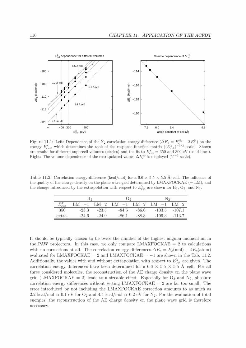
116 CHAPTER 11. APPLICATION OF THE ACFDT
-120
-115
-110
-105
-100
∞ 200300400
∆Ec
(kca
l/mol
)
Eχcut (eV)
Eχcut dependence for different volumes
A6.6 cell
A6.0 cell
A5.4 cell
A4.8 cell
A7.2 cell
−120
−118
−116
−114
4.85.46.07.2∆E
c (k
cal/m
ol)
lattice constant of cell (Å)
Volume dependence of ∆Ec∞
Figure 11.1: Left: Dependence of the N2 correlation energy difference (∆Ec = EN2
c − 2ENc ) on the
energy Eχcut, which determines the rank of the response function matrix [(Eχ
cut)−3/2 scale]. Shown
are results for different supercell volumes (circles) and the fit to Eχcut = 350 and 300 eV (solid lines).
Right: The volume dependence of the extrapolated values ∆E∞
c is displayed (V −2 scale).
Table 11.2: Correlation energy difference (kcal/mol) for a 6.6 × 5.5 × 5.5 A cell. The influence ofthe quality of the charge density on the plane wave grid determined by LMAXFOCKAE (= LM), andthe change introduced by the extrapolation with respect to Eχ
cut are shown for H2, O2, and N2.
H2 O2 N2
Eχcut LM=−1 LM=2 LM=−1 LM=2 LM=−1 LM=2
350 -23.3 -23.5 -84.5 -86.6 -103.5 -107.1extra. -24.6 -24.9 -86.1 -88.3 -109.3 -113.7
It should be typically chosen to be twice the number of the highest angular momentum inthe PAW projectors. In this case, we only compare LMAXFOCKAE = 2 to calculationswith no corrections at all. The correlation energy differences ∆Ec = Ec(mol) − 2Ec(atom)evaluated for LMAXFOCKAE = 2 and LMAXFOCKAE = −1 are shown in the Tab. 11.2.Additionally, the values with and without extrapolation with respect to Eχ
cut are given. Thecorrelation energy differences have been determined for a 6.6 × 5.5 × 5.5 A cell. For allthree considered molecules, the reconstruction of the AE charge density on the plane wavegrid (LMAXFOCKAE = 2) leads to a sizeable effect. Especially for O2 and N2, absolutecorrelation energy differences without setting LMAXFOCKAE = 2 are far too small. Theerror introduced by not including the LMAXFOCKAE correction amounts to as much as2.2 kcal/mol ≈ 0.1 eV for O2 and 4.4 kcal/mol ≈ 0.2 eV for N2. For the evaluation of totalenergies, the reconstruction of the AE charge density on the plane wave grid is thereforenecessary.
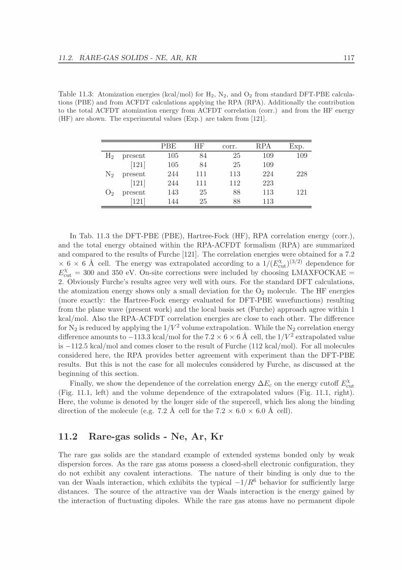
11.2. RARE-GAS SOLIDS - NE, AR, KR 117
Table 11.3: Atomization energies (kcal/mol) for H2, N2, and O2 from standard DFT-PBE calcula-tions (PBE) and from ACFDT calculations applying the RPA (RPA). Additionally the contributionto the total ACFDT atomization energy from ACFDT correlation (corr.) and from the HF energy(HF) are shown. The experimental values (Exp.) are taken from [121].
PBE HF corr. RPA Exp.
H2 present 105 84 25 109 109[121] 105 84 25 109
N2 present 244 111 113 224 228[121] 244 111 112 223
O2 present 143 25 88 113 121[121] 144 25 88 113
In Tab. 11.3 the DFT-PBE (PBE), Hartree-Fock (HF), RPA correlation energy (corr.),and the total energy obtained within the RPA-ACFDT formalism (RPA) are summarizedand compared to the results of Furche [121]. The correlation energies were obtained for a 7.2× 6 × 6 A cell. The energy was extrapolated according to a 1/(Eχ
cut)(3/2) dependence for
Eχcut = 300 and 350 eV. On-site corrections were included by choosing LMAXFOCKAE =
2. Obviously Furche’s results agree very well with ours. For the standard DFT calculations,the atomization energy shows only a small deviation for the O2 molecule. The HF energies(more exactly: the Hartree-Fock energy evaluated for DFT-PBE wavefunctions) resultingfrom the plane wave (present work) and the local basis set (Furche) approach agree within 1kcal/mol. Also the RPA-ACFDT correlation energies are close to each other. The differencefor N2 is reduced by applying the 1/V 2 volume extrapolation. While the N2 correlation energydifference amounts to −113.3 kcal/mol for the 7.2 × 6 × 6 A cell, the 1/V 2 extrapolated valueis −112.5 kcal/mol and comes closer to the result of Furche (112 kcal/mol). For all moleculesconsidered here, the RPA provides better agreement with experiment than the DFT-PBEresults. But this is not the case for all molecules considered by Furche, as discussed at thebeginning of this section.
Finally, we show the dependence of the correlation energy ∆Ec on the energy cutoff Eχcut
(Fig. 11.1, left) and the volume dependence of the extrapolated values (Fig. 11.1, right).Here, the volume is denoted by the longer side of the supercell, which lies along the bindingdirection of the molecule (e.g. 7.2 A cell for the 7.2 × 6.0 × 6.0 A cell).
11.2 Rare-gas solids - Ne, Ar, Kr
The rare gas solids are the standard example of extended systems bonded only by weakdispersion forces. As the rare gas atoms possess a closed-shell electronic configuration, theydo not exhibit any covalent interactions. The nature of their binding is only due to thevan der Waals interaction, which exhibits the typical −1/R6 behavior for sufficiently largedistances. The source of the attractive van der Waals interaction is the energy gained bythe interaction of fluctuating dipoles. While the rare gas atoms have no permanent dipole
118 CHAPTER 11. APPLICATION OF THE ACFDT
moment, quantum fluctuations introduce an instantaneous dipole moment. In a qualitativepicture of two atoms at a distance R, the dipole moment on atom 1, p1, results in an electricfield E ∝ p1/R
3. The electric field introduces a dipole moment on atom 2, p2, which isproportional to the electric field p2 ∝ E(R) ∝ p1/R
3. The energy of a dipole moment in anelectric field is given by V = −p2E which, in total, results in a potential V ∝ −p1p2/R
6.How strongly an atom can be polarized by an electric field depends on its polarizability.Consequently, this quantity enters the van der Waals potential as a prefactor.
The nature of the van der Waals interaction is non-local, because it describes the reactionof an atom at position r to the density fluctuations of a second atom at position r′. Sucha correlation contribution is not captured in any local (LDA) or semilocal (GGA) approxi-mation of the correlation energy as normally used in DFT calculations (see also Ref. [32]).This failure of standard DFT becomes evident in the description of rare gas molecules andsolids, where LDA strongly overbinds, while GGA underbinds. Other prominent examplesare graphite and h-BN, for which GGA does not provide an interlayer binding between thegraphene and h-BN sheets at all, while LDA binds only because of a spurious cancellation oferrors in the description of the exchange and correlation energy. Therefore, it is common to
include the van der Waals potential as an additional energy contribution ∝ C(ab)6 /R6
(ab), and
to sum over all pairs of atoms (a, b) present in the system (see e.g., [135]). In order to avoidstrong interactions at very small distances, the 1/R6 potential is damped for small values ofR. This approach thus resembles the introduction of a Lennard-Jones potential:
Vab(Rab) =Cab
12
R12ab
−Cab
6
R6ab
(11.2)
The coefficient C6 can be calculated from the ab-initio atomic polarizability.
Beside the difficulties of determining the damping factor and the correct calculation ofthe atomic polarizability, a fundamental problem lies in the assumption that the correct Rdependence of the correlation can be obtained by summing over terms of the form given inEq. (11.2). While the summation over the 1/R6 terms gives the correct energy behavior inleading order of 1/R (not necessarily the correct prefactors) for an insulating system, it canbe shown [32, 33] that for metals not even the correct long-range behavior can be reproduced.Thus, this semi-empirical treatment can not be the proper solution for the description of vander Waals bonded systems.
The ACFDT formulism provides an exact (non-local) expression for the correlation energy,and therefore naturally also includes the van der Waals interaction. Even within the RPA,it has been shown [34] that the correct long-range 1/R6 behavior for two atoms (respectivelythe correct dependence on the distance R for any system) can be reproduced. Only thecoefficients are altered by the RPA approximation, so that e.g., the C6 coefficients describingthe interaction between two distant atoms are determined by the RPA atomic polarizabilitiesinstead of the exact ones.
In this chapter, we will present RPA cohesive energies for the fcc rare-gas crystals of Ne,Ar, and Kr. The applied potentials were generated as to guarantee good scattering propertiesfor the isolated atoms for up to ≈ 10 Ry. The parameters of these potentials are summarizedin Tab. 11.4. For the Hartree-Fock energy, EHF , a 12× 12× 12 k-point grid was used. Thisdense k-point grid was necessary in order to obtain convergence on the meV level. For theRPA correlation energies, a 6× 6× 6 k-point grid already leads to relatively smooth energy-
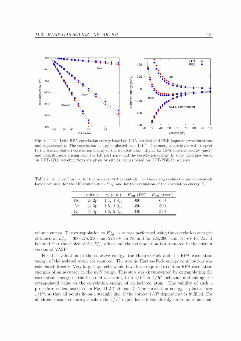
11.2. RARE-GAS SOLIDS - NE, AR, KR 119
−0.6
−0.5
−0.4
−0.3
−0.2
−0.1
0.0
304050100 25
corr
elat
ion
ener
gy (
eV)
Volume (ų)
Neon
Argon
Krypton
−600
−400
−200
0
200
400
20 30 40 50 60 70 80 90 100co
hesi
ve e
nerg
y (m
eV)
volume (ų)
ACFDT correlation
HF
total
LDAPBE
Figure 11.2: Left: RPA correlation energy based on LDA (circles) and PBE (squares) wavefunctionsand eigenenergies. The correlation energy is plotted over 1/V 2. The energies are given with respectto the (extrapolated) correlation energy of the isolated atom. Right: Kr RPA cohesive energy (meV)and contributions arising from the HF part EHF and the correlation energy Ec only. Energies basedon DFT-LDA wavefunctions are given by circles, values based on DFT-PBE by squares.
Table 11.4: Cutoff radii rc for the rare gas PAW potentials. For the rare gas solids the same potentialshave been used for the HF contribution EHF and for the evaluation of the correlation energy Ec.
valence rc (a.u.) Ecut (HF) Ecut (corr.)
Ne 2s 2p 1.4s 1.8pd 900 650Ar 3s 3p 1.5s 1.9pd 390 390Kr 4s 4p 1.8s 2.3pd 340 340
volume curves. The extrapolation to Eχcut →∞ was performed using the correlation energies
obtained at Eχcut = 300, 275, 250, and 225 eV for Ne and for 225, 200, and 175 eV for Ar. It
is noted that the choice of the Eχcut values and the extrapolation is automated in the current
version of VASP.
For the evaluation of the cohesive energy, the Hartree-Fock and the RPA correlationenergy of the isolated atom are required. The atomic Hartree-Fock energy contribution wascalculated directly. Very large supercells would have been required to obtain RPA correlationenergies of an accuracy in the meV range. This step was circumvented by extrapolating thecorrelation energy of the fcc solid according to a 1/V 2 ∝ 1/R6 behavior and taking theextrapolated value as the correlation energy of an isolated atom. The validity of such aprocedure is demonstrated in Fig. 11.2 (left panel). The correlation energy is plotted over1/V 2, so that all points lie on a straight line, if the correct 1/R6 dependence is fulfilled. Forall three considered rare gas solids the 1/V 2 dependence holds already for volumes as small
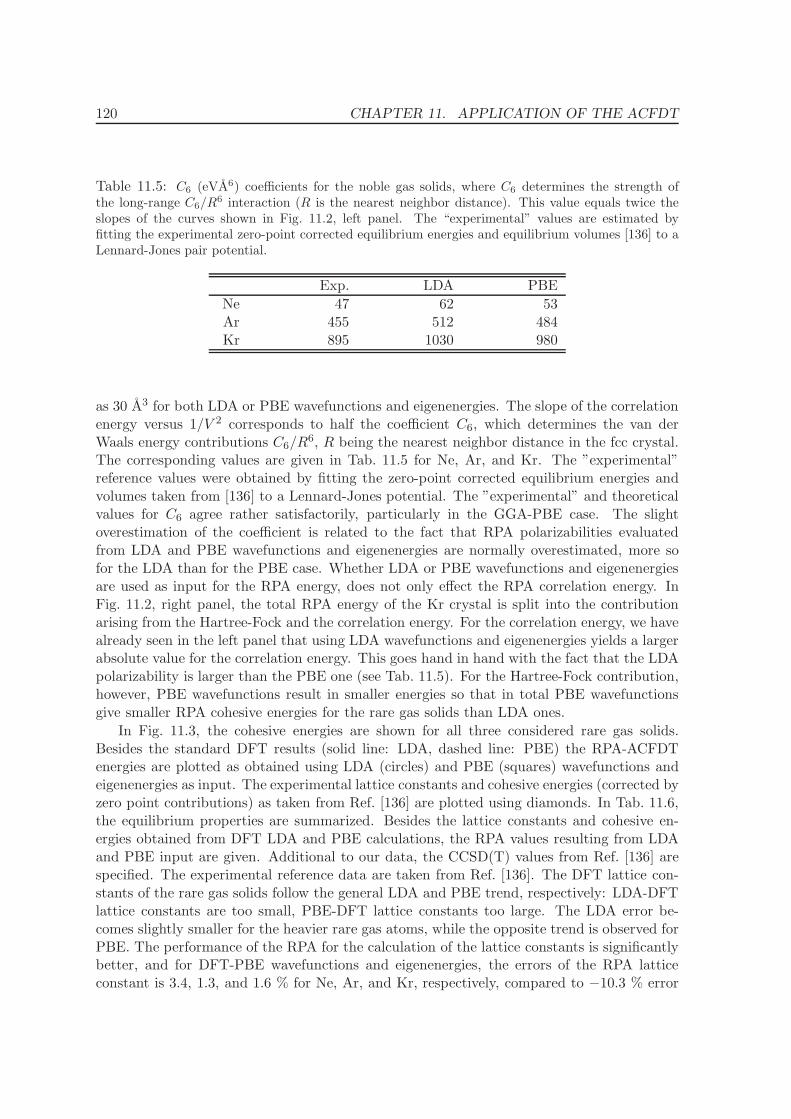
120 CHAPTER 11. APPLICATION OF THE ACFDT
Table 11.5: C6 (eVA6) coefficients for the noble gas solids, where C6 determines the strength ofthe long-range C6/R
6 interaction (R is the nearest neighbor distance). This value equals twice theslopes of the curves shown in Fig. 11.2, left panel. The “experimental” values are estimated byfitting the experimental zero-point corrected equilibrium energies and equilibrium volumes [136] to aLennard-Jones pair potential.
Exp. LDA PBE
Ne 47 62 53Ar 455 512 484Kr 895 1030 980
as 30 A3 for both LDA or PBE wavefunctions and eigenenergies. The slope of the correlationenergy versus 1/V 2 corresponds to half the coefficient C6, which determines the van derWaals energy contributions C6/R
6, R being the nearest neighbor distance in the fcc crystal.The corresponding values are given in Tab. 11.5 for Ne, Ar, and Kr. The ”experimental”reference values were obtained by fitting the zero-point corrected equilibrium energies andvolumes taken from [136] to a Lennard-Jones potential. The ”experimental” and theoreticalvalues for C6 agree rather satisfactorily, particularly in the GGA-PBE case. The slightoverestimation of the coefficient is related to the fact that RPA polarizabilities evaluatedfrom LDA and PBE wavefunctions and eigenenergies are normally overestimated, more sofor the LDA than for the PBE case. Whether LDA or PBE wavefunctions and eigenenergiesare used as input for the RPA energy, does not only effect the RPA correlation energy. InFig. 11.2, right panel, the total RPA energy of the Kr crystal is split into the contributionarising from the Hartree-Fock and the correlation energy. For the correlation energy, we havealready seen in the left panel that using LDA wavefunctions and eigenenergies yields a largerabsolute value for the correlation energy. This goes hand in hand with the fact that the LDApolarizability is larger than the PBE one (see Tab. 11.5). For the Hartree-Fock contribution,however, PBE wavefunctions result in smaller energies so that in total PBE wavefunctionsgive smaller RPA cohesive energies for the rare gas solids than LDA ones.
In Fig. 11.3, the cohesive energies are shown for all three considered rare gas solids.Besides the standard DFT results (solid line: LDA, dashed line: PBE) the RPA-ACFDTenergies are plotted as obtained using LDA (circles) and PBE (squares) wavefunctions andeigenenergies as input. The experimental lattice constants and cohesive energies (corrected byzero point contributions) as taken from Ref. [136] are plotted using diamonds. In Tab. 11.6,the equilibrium properties are summarized. Besides the lattice constants and cohesive en-ergies obtained from DFT LDA and PBE calculations, the RPA values resulting from LDAand PBE input are given. Additional to our data, the CCSD(T) values from Ref. [136] arespecified. The experimental reference data are taken from Ref. [136]. The DFT lattice con-stants of the rare gas solids follow the general LDA and PBE trend, respectively: LDA-DFTlattice constants are too small, PBE-DFT lattice constants too large. The LDA error be-comes slightly smaller for the heavier rare gas atoms, while the opposite trend is observed forPBE. The performance of the RPA for the calculation of the lattice constants is significantlybetter, and for DFT-PBE wavefunctions and eigenenergies, the errors of the RPA latticeconstant is 3.4, 1.3, and 1.6 % for Ne, Ar, and Kr, respectively, compared to −10.3 % error

11.2. RARE-GAS SOLIDS - NE, AR, KR 121
−150
−100
−50
0
50
20 30 40 50 60 70 80 90
cohe
sive
ene
rgy
(meV
)
volume (ų)
Argon
LDAPBE
ACFDT LDAACFDT PBE
−200
−150
−100
−50
0
50
100
20 30 40 50 60 70 80 90 100
cohe
sive
ene
rgy
(meV
)
volume (ų)
Krypton
LDAPBE
ACFDT LDAACFDT PBE
−100
−80
−60
−40
−20
0
20
10 15 20 25 30 35 40 45 50
cohe
sive
ene
rgy
(meV
)
volume (ų)
Neon
LDAPBE
ACFDT LDAACFDT PBE
Figure 11.3: Cohesive energy (meV) as a function of the primitive cell volume for the fcc noble gascrystals Ne, Ar, and Kr. Besides the cohesive energies obtained from the RPA-ACFDT calculationsbased on LDA (circles) and PBE (squares) wavefunctions and eigenenergies, standard DFT resultswithin the LDA (solid line) and PBE (dashed line) are shown. The experimental values (withoutzero-point energy) are given by black diamonds.
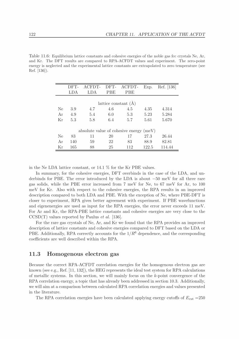
122 CHAPTER 11. APPLICATION OF THE ACFDT
Table 11.6: Equilibrium lattice constants and cohesive energies of the noble gas fcc crystals Ne, Ar,and Kr. The DFT results are compared to RPA-ACFDT values and experiment. The zero-pointenergy is neglected and the experimental lattice constants are extrapolated to zero temperature (seeRef. [136]).
DFT- ACFDT- DFT- ACFDT- Exp. Ref. [136]LDA LDA PBE PBE
lattice constant (A)Ne 3.9 4.7 4.6 4.5 4.35 4.314Ar 4.9 5.4 6.0 5.3 5.23 5.284Kr 5.3 5.8 6.4 5.7 5.61 5.670
absolute value of cohesive energy (meV)Ne 83 11 20 17 27.3 26.44Ar 140 59 22 83 88.9 82.81Kr 165 88 25 112 122.5 114.44
in the Ne LDA lattice constant, or 14.1 % for the Kr PBE values.
In summary, for the cohesive energies, DFT overbinds in the case of the LDA, and un-derbinds for PBE. The error introduced by the LDA is about −50 meV for all three raregas solids, while the PBE error increased from 7 meV for Ne, to 67 meV for Ar, to 100meV for Kr. Also with respect to the cohesive energies, the RPA results in an improveddescription compared to both LDA and PBE. With the exception of Ne, where PBE-DFT iscloser to experiment, RPA gives better agreement with experiment. If PBE wavefunctionsand eigenenergies are used as input for the RPA energies, the error never exceeds 11 meV.For Ar and Kr, the RPA-PBE lattice constants and cohesive energies are very close to theCCSD(T) values reported by Paulus et al. [136].
For the rare gas crystals of Ne, Ar, and Kr we found that the RPA provides an improveddescription of lattice constants and cohesive energies compared to DFT based on the LDA orPBE. Additionally, RPA correctly accounts for the 1/R6 dependence, and the correspondingcoefficients are well described within the RPA.
11.3 Homogenous electron gas
Because the correct RPA-ACFDT correlation energies for the homogenous electron gas areknown (see e.g., Ref. [11, 132]), the HEG represents the ideal test system for RPA calculationsof metallic systems. In this section, we will mainly focus on the k-point convergence of theRPA correlation energy, a topic that has already been addressed in section 10.3. Additionally,we will aim at a comparison between calculated RPA correlation energies and values presentedin the literature.
The RPA correlation energies have been calculated applying energy cutoffs of Ecut =250
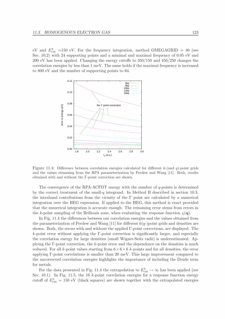
11.3. HOMOGENOUS ELECTRON GAS 123
eV and Eχcut =150 eV. For the frequency integration, method OMEGAGRID = 40 (see
Sec. 10.2) with 24 supporting points and a minimal and maximal frequency of 0.05 eV and200 eV has been applied. Changing the energy cutoffs to 350/150 and 450/250 changes thecorrelation energies by less than 1 meV. The same holds if the maximal frequency is increasedto 800 eV and the number of supporting points to 64.
0.00
0.02
0.04
0.06
0.08
0.10
0.12
1.8 2.0 2.2 2.4 2.6 2.8 3.0
erro
r in
ene
rgy
(eV
)
rs (a.u.)
6kp8kp
10kp12kp16kp
No Γ point correction
Figure 11.4: Difference between correlation energies calculated for different k-(and q)-point gridsand the values stemming from the RPA parameterization by Perdew and Wang [11]. Both, resultsobtained with and without the Γ-point correction are shown.
The convergence of the RPA-ACFDT energy with the number of q-points is determinedby the correct treatment of the small-q integrand. In Method B described in section 10.3,the intraband contributions from the vicinity of the Γ point are calculated by a numericalintegration over the HEG expression. If applied to the HEG, this method is exact providedthat the numerical integration is accurate enough. The remaining error stems from errors inthe k-point sampling of the Brillouin zone, when evaluating the response function χ(q).
In Fig. 11.4 the differences between our correlation energies and the values obtained fromthe parameterization of Perdew and Wang [11] for different k(q-)point grids and densities areshown. Both, the errors with and without the applied Γ-point corrections, are displayed. Thek-point error without applying the Γ-point correction is significantly larger, and especiallythe correlation energy for large densities (small Wigner-Seitz radii) is underestimated. Ap-plying the Γ-point correction, the k-point error and the dependence on the densities is muchreduced. For all k-point values starting from 6×6×6 k-points and for all densities, the errorapplying Γ-point correlations is smaller than 20 meV. This large improvement compared tothe uncorrected correlation energies highlights the importance of including the Drude termfor metals.
For the data presented in Fig. 11.4 the extrapolation to Eχcut →∞ has been applied (see
Sec. 10.1). In Fig. 11.5, the 16 k-point correlation energies for a response function energycutoff of Eχ
cut = 150 eV (black squares) are shown together with the extrapolated energies
124 CHAPTER 11. APPLICATION OF THE ACFDT
with (empty circles) and without (empty squares) applying the Γ-point correction. Evidently,the Eχ
cut extrapolation is essential in order to obtain accurate correlation energies.
The number of points used in the frequency integration (NOMEGA) could play a moreimportant role for metals than for semiconductors due to the existence of small frequencytransitions. Although the Drude term is treated separately (as done in Method B), a dense q-point grid will lead to small q-point transitions and consequently small intraband excitations.Nevertheless, we found that the frequency integration is unproblematic, at least in the caseof the HEG. If the integration scheme OMEGAGRID = 4 is used (see Sec. 10.2), convergedenergies are obtained already for 16 frequency points. We therefore observe that the intrabandcontributions are well manageable. Only if band crossings occur near the Fermi surface, asfor Al and the transition metals, faster convergence is obtained if extremely small frequencypoints are not considered (see next section).
-1.9
-1.8
-1.7
-1.6
-1.5
-1.4
-1.3
1.5 2.0 2.5 3.0 3.5
RP
A c
orre
latio
n en
ergy
(eV
)
rs (a.u.)
Perdew-Wang parametrizationpresent
no Γ correctionno Ecut
χ correction, no Γ correction
Figure 11.5: Influence of the Eχcut extrapolation and of the Γ-point correction on the HEG
RPA correlation energy.
Finally we address the reproducibility of published data with our implementation ofthe RPA energy in VASP. Published data for the HEG RPA correlation energy [132] werecalculated numerically by evaluating Eq. (10.1). Here, we compare to the parameterizationof the HEG RPA correlation energies as provided by Perdew and Wang [11]. Our calculationshave been performed for densities corresponding to Wigner-Seitz radii between 1.75 and 3.0.The energy cutoff Ecut was chosen to be 250 eV and for the response function plane wavecomponents with an energy of up to Eχ
cut = 150 eV were considered. The Eχcut extrapolation
was performed as described in Sec 10.1. The final RPA correlation energies (empty circlesin Fig. 11.5) stem from a 16 k-point calculation and the Γ point correction was applied. Forthe frequency integration the scheme OMEGAGRID = 40 was employed and the smallestfrequency was chosen to be SIGMA = 0.05 eV. For all considered densities the differencebetween our calculated RPA correlation energies and the literature values [11] is smallerthan 9 meV.
11.4. METALS - NA, AL, CU, RH, PD 125
11.4 Metals - Na, Al, Cu, Rh, Pd
In this section, RPA calculations of the metals Na, Cu, Al, Rh, and Pd will be presented.We will focus on the convergence of the lattice constant, the bulk modulus, and the totalenergy with respect to the k-point grid used in the evaluation of the HF energy and theRPA-ACFDT correlation energy. Additionally, the influence of the Γ-point correction (=inclusion of the Drude term) for the RPA correlation energy (see Sec. 10.3) is investigatedfor all five metals. We have applied the same energy cutoffs Ecut and Eχ
cut as specified inTab. 11.9. The parameters of the frequency integration, the integration method, the numberof frequency points, and the maximal/minimal frequency are also summarized in Tab. 11.9.For Na, we used a PAW potential that treats only the 3s electrons as valence, referred to asNa1 potential in section 11.5.
In the previous section, the RPA correlation energy of the homogenous electron gas (HEG)has been calculated and the inclusion of the Γ-point corrections was found to significantlyimprove the k-point convergence. As sodium can be considered to be a nearly free electronlike metal, the Na bcc crystal represents the first step from the HEG to a real metallic system.The total energy (EHF + Ec) of the Na bcc crystal is shown in Fig. 11.6. Three differentcases are considered: In the top panel, the RPA correlation energy is not corrected for bythe Γ-point contributions and the HF energy is always evaluated using a 16×16×16 k-pointgrid. In the middle panel, the HF part is treated as before, but the Γ-point correction isadded to the RPA correlation energy. In the bottom panel, the HF part is calculated usingthe same k-point grid as employed for the correlation energy, and the Γ-point correction isapplied. The lattice constants, bulk moduli, and total energies of Na and the other metalsare summarized in Tab. 11.7. If no Γ-point correction is added and a 16 × 16 × 16 k-pointgrid is considered for the HF energy (top panel of Fig. 11.6), the energy error is dominatedby errors in the correlation energy. The general form of the Na energy versus volume curveis basically maintained for all chosen k-point grids, with a slight overestimation of the latticeconstant for coarser grids. The absolute value of the correlation energy is too small for a6×6×6 k-point grid (by ≈ 70 meV) and continously increases towards a denser k-point grid.Adding the Γ-point correction (middle panel of Fig. 11.6), leads to a significant improvementof the energy convergence (30 meV error for 6×6×6 k-points, < 10 meV for more k-points.)The k-point error for the lattice constants also decreases. If the HF energy is evaluatedat a 16 × 16 × 16 grid, and Γ-point corrections are applied for the correlation energy, thelattice constant stemming from the 8× 8× 8 k-point correlation energy differs only by 0.05% from the converged result. The error in the total energy only amounts to 7 meV. Muchslower convergence of the lattice constants and energies is obtained, if the same k-pointgrid is applied for the HF and the correlation energy. The resulting energy-volume curvesare presented in the bottom panel of Fig. 11.6. The difference between the 8 × 8 × 8 and16 × 16 × 16 k-point lattice constants now amounts to 0.2 % and the total energy varies by25 meV.
For Cu, the lattice constants and total energies calculated with and without Γ-pointcorrection and different k-point settings for the HF part are summarized in Tab. 11.7. Incontrast to Na, both the valence s-electron and the d-electrons contribute to the correlationenergy of the Cu fcc crystal. As a consequence, the Drude like contribution around theΓ-point is not as dominant as in the case of Na. Even without considering the Γ-point
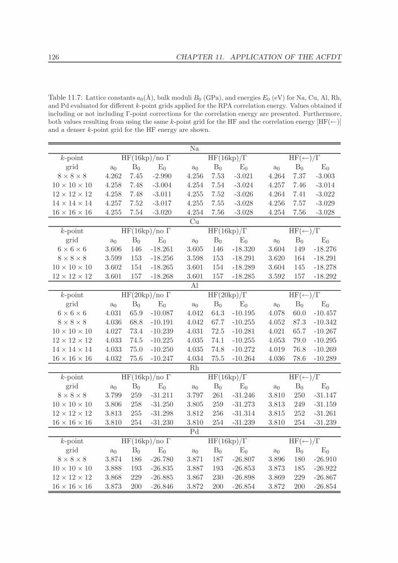
126 CHAPTER 11. APPLICATION OF THE ACFDT
Table 11.7: Lattice constants a0(A), bulk moduli B0 (GPa), and energies E0 (eV) for Na, Cu, Al, Rh,and Pd evaluated for different k-point grids applied for the RPA correlation energy. Values obtained ifincluding or not including Γ-point corrections for the correlation energy are presented. Furthermore,both values resulting from using the same k-point grid for the HF and the correlation energy [HF(←)]and a denser k-point grid for the HF energy are shown.
Na
k-point HF(16kp)/no Γ HF(16kp)/Γ HF(←)/Γgrid a0 B0 E0 a0 B0 E0 a0 B0 E0
8× 8× 8 4.262 7.45 -2.990 4.256 7.53 -3.021 4.264 7.37 -3.00310× 10× 10 4.258 7.48 -3.004 4.254 7.54 -3.024 4.257 7.46 -3.01412× 12× 12 4.258 7.48 -3.011 4.255 7.52 -3.026 4.264 7.41 -3.02214× 14× 14 4.257 7.52 -3.017 4.255 7.55 -3.028 4.256 7.57 -3.02916× 16× 16 4.255 7.54 -3.020 4.254 7.56 -3.028 4.254 7.56 -3.028
Cu
k-point HF(16kp)/no Γ HF(16kp)/Γ HF(←)/Γgrid a0 B0 E0 a0 B0 E0 a0 B0 E0
6× 6× 6 3.606 146 -18.261 3.605 146 -18.320 3.604 149 -18.2768× 8× 8 3.599 153 -18.256 3.598 153 -18.291 3.620 164 -18.291
10× 10× 10 3.602 154 -18.265 3.601 154 -18.289 3.604 145 -18.27812× 12× 12 3.601 157 -18.268 3.601 157 -18.285 3.592 157 -18.292
Al
k-point HF(20kp)/no Γ HF(20kp)/Γ HF(←)/Γgrid a0 B0 E0 a0 B0 E0 a0 B0 E0
6× 6× 6 4.031 65.9 -10.087 4.042 64.3 -10.195 4.078 60.0 -10.4578× 8× 8 4.036 68.8 -10.191 4.042 67.7 -10.255 4.052 87.3 -10.342
10× 10× 10 4.027 73.4 -10.239 4.031 72.5 -10.281 4.021 65.7 -10.26712× 12× 12 4.033 74.5 -10.225 4.035 74.1 -10.255 4.053 79.0 -10.29514× 14× 14 4.033 75.0 -10.250 4.035 74.8 -10.272 4.019 76.8 -10.26916× 16× 16 4.032 75.6 -10.247 4.034 75.5 -10.264 4.036 78.6 -10.289
Rh
k-point HF(16kp)/no Γ HF(16kp)/Γ HF(←)/Γgrid a0 B0 E0 a0 B0 E0 a0 B0 E0
8× 8× 8 3.799 259 -31.211 3.797 261 -31.246 3.810 250 -31.14710× 10× 10 3.806 258 -31.250 3.805 259 -31.273 3.813 249 -31.15912× 12× 12 3.813 255 -31.298 3.812 256 -31.314 3.815 252 -31.26116× 16× 16 3.810 254 -31.230 3.810 254 -31.239 3.810 254 -31.239
Pd
k-point HF(16kp)/no Γ HF(16kp)/Γ HF(←)/Γgrid a0 B0 E0 a0 B0 E0 a0 B0 E0
8× 8× 8 3.874 186 -26.780 3.871 187 -26.807 3.896 180 -26.91010× 10× 10 3.888 193 -26.835 3.887 193 -26.853 3.873 185 -26.92212× 12× 12 3.868 229 -26.885 3.867 230 -26.898 3.869 229 -26.86716× 16× 16 3.873 200 -26.846 3.872 200 -26.854 3.872 200 -26.854
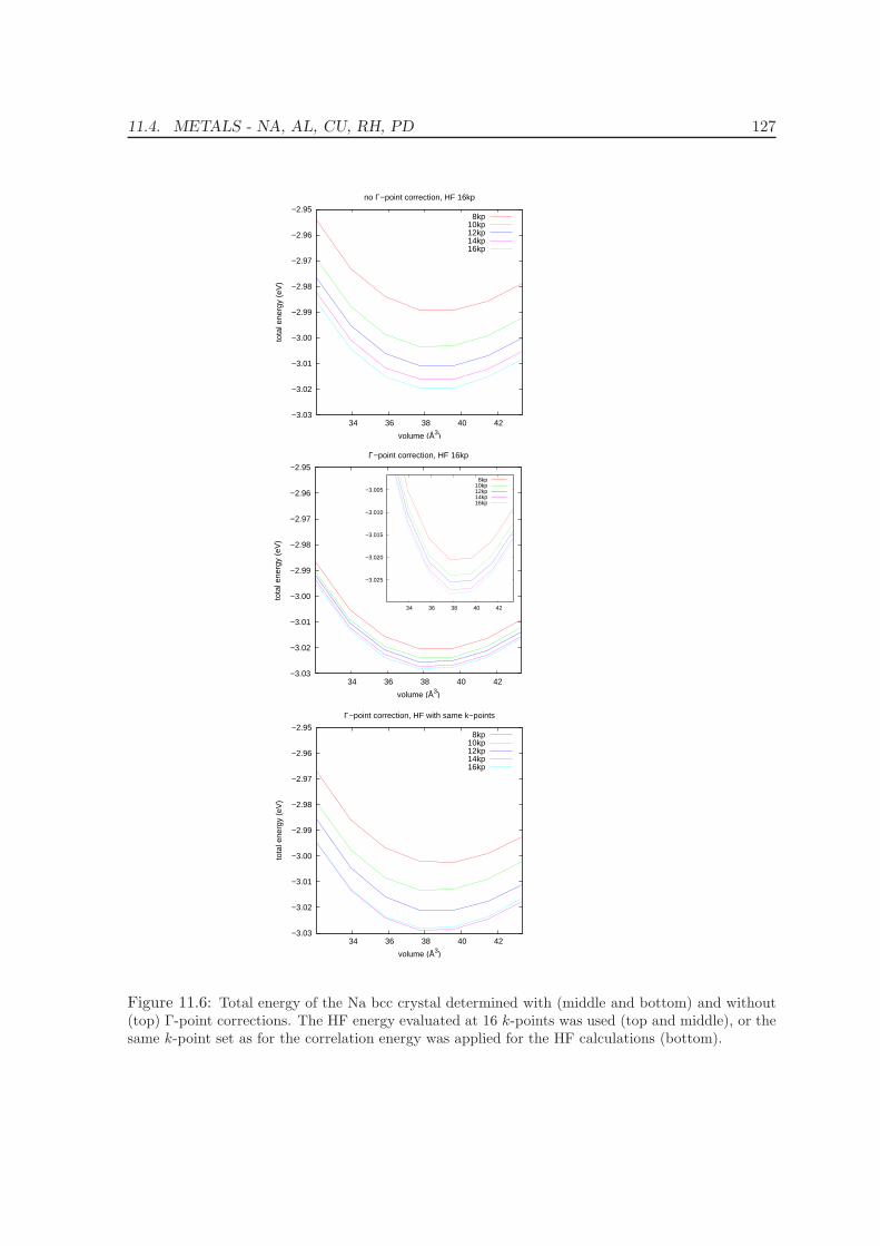
11.4. METALS - NA, AL, CU, RH, PD 127
−3.03
−3.02
−3.01
−3.00
−2.99
−2.98
−2.97
−2.96
−2.95
34 36 38 40 42
tota
l ene
rgy
(eV
)
volume (Å3)
no Γ−point correction, HF 16kp
8kp10kp12kp14kp16kp
−3.03
−3.02
−3.01
−3.00
−2.99
−2.98
−2.97
−2.96
−2.95
34 36 38 40 42
tota
l ene
rgy
(eV
)
volume (Å3)
Γ−point correction, HF 16kp
8kp10kp12kp14kp16kp
−3.025
−3.020
−3.015
−3.010
−3.005
34 36 38 40 42
8kp10kp12kp14kp16kp
−3.03
−3.02
−3.01
−3.00
−2.99
−2.98
−2.97
−2.96
−2.95
34 36 38 40 42
tota
l ene
rgy
(eV
)
volume (Å3)
Γ−point correction, HF with same k−points
8kp10kp12kp14kp16kp
Figure 11.6: Total energy of the Na bcc crystal determined with (middle and bottom) and without(top) Γ-point corrections. The HF energy evaluated at 16 k-points was used (top and middle), or thesame k-point set as for the correlation energy was applied for the HF calculations (bottom).
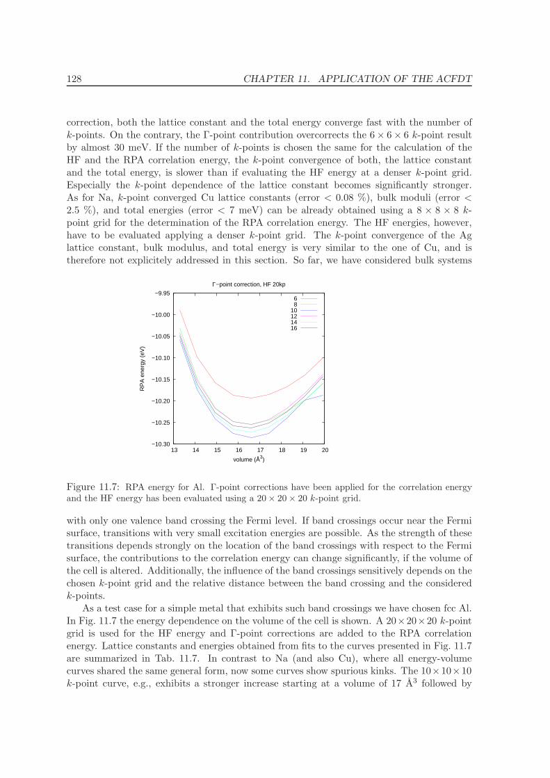
128 CHAPTER 11. APPLICATION OF THE ACFDT
correction, both the lattice constant and the total energy converge fast with the number ofk-points. On the contrary, the Γ-point contribution overcorrects the 6× 6× 6 k-point resultby almost 30 meV. If the number of k-points is chosen the same for the calculation of theHF and the RPA correlation energy, the k-point convergence of both, the lattice constantand the total energy, is slower than if evaluating the HF energy at a denser k-point grid.Especially the k-point dependence of the lattice constant becomes significantly stronger.As for Na, k-point converged Cu lattice constants (error < 0.08 %), bulk moduli (error <2.5 %), and total energies (error < 7 meV) can be already obtained using a 8 × 8 × 8 k-point grid for the determination of the RPA correlation energy. The HF energies, however,have to be evaluated applying a denser k-point grid. The k-point convergence of the Aglattice constant, bulk modulus, and total energy is very similar to the one of Cu, and istherefore not explicitely addressed in this section. So far, we have considered bulk systems
−10.30
−10.25
−10.20
−10.15
−10.10
−10.05
−10.00
−9.95
13 14 15 16 17 18 19 20
RP
A e
nerg
y (e
V)
volume (Å3)
Γ−point correction, HF 20kp
68
10121416
Figure 11.7: RPA energy for Al. Γ-point corrections have been applied for the correlation energyand the HF energy has been evaluated using a 20× 20× 20 k-point grid.
with only one valence band crossing the Fermi level. If band crossings occur near the Fermisurface, transitions with very small excitation energies are possible. As the strength of thesetransitions depends strongly on the location of the band crossings with respect to the Fermisurface, the contributions to the correlation energy can change significantly, if the volume ofthe cell is altered. Additionally, the influence of the band crossings sensitively depends on thechosen k-point grid and the relative distance between the band crossing and the consideredk-points.
As a test case for a simple metal that exhibits such band crossings we have chosen fcc Al.In Fig. 11.7 the energy dependence on the volume of the cell is shown. A 20×20×20 k-pointgrid is used for the HF energy and Γ-point corrections are added to the RPA correlationenergy. Lattice constants and energies obtained from fits to the curves presented in Fig. 11.7are summarized in Tab. 11.7. In contrast to Na (and also Cu), where all energy-volumecurves shared the same general form, now some curves show spurious kinks. The 10×10×10k-point curve, e.g., exhibits a stronger increase starting at a volume of 17 A3 followed by
11.4. METALS - NA, AL, CU, RH, PD 129
a kink at 19 A3. A similar behavior can be observed for the 8 × 8 × 8 k-point grid. Thekinks in these energy-volume curves are large enough to question if fits to the 8× 8× 8 and10 × 10 × 10 k-point curves are meaningful at all. Furthermore, the k-point convergence ofthe Al HF energies is especially slow. If the same k-point grids are applied for the HF andthe correlation energy, the lattice constant changes by 0.4 % for different k-point grids andthe error in the energy is also significantly larger than for a dense HF k-point grid.
Finally, we consider the convergence of lattice constants and total energies for the transi-tion metals Rh and Pd. Both metals have only partially filled 3d states and due to the largenumber of d bands near the Fermi level the effect caused by band crossings is even strongerthan for Al. The k-point convergence is indeed harder to achieve for Rh and Pd than forall other metals considered so far. For Al, we have found that the energy volume curve canexhibit spurious kinks for specific k-point grids, but the k-point convergence of the latticeconstant, the bulk modulus, and the total energy was nevertheless reasonable fast. For thetransition metals, the lattice constants undergo larger variations for different k-point gridsthan was the case for the other considered metals, and for Pd a 12 × 12 × 12 k-point gridleads to a significantly altered shape of the energy-volume curve with a bulk modulus whichis 13 % off the values obtained for the other k-point settings. Also the k-point convergenceof the Rh and Pd total energy is slower than for the other considered metals. If the HFenergy is evaluated applying a dense k-point mesh, the energy difference for using a 8× 8× 8or 12 × 12 × 12 k-point grid for the evaluation of the correlation energy amounts to 70 and90 meV for Rh and Pd, respectively. The same difference is only 5 meV for Na and 6 meVfor Cu. In contrast to the other metals, the k-point dependence of the total energy is notworsened, if the HF energy is evaluated applying the same k-point grid as used for the RPAcorrelation energy.
The spurious influence of transitions between states with small energy differences can besomewhat diminished by avoiding to evaluate the response function for very small frequencies.This can be done by choosing the first supporting point for the frequency integration relativelylarge. To this end, the frequency integration scheme OMEGAGRID = 40 (see Sec. 10.2) hasbeen applied which allows to set the smallest frequency by SIGMA. We found that SIGMA= 0.2 eV reduces the effect of the small energy transitions and at the same time seems tocapture most of the ”desirable” part of the correlation energy.
We have found that for both, Na and Cu, the k-point convergence of the lattice constant,the bulk modulus, and the total energy is unproblematic. For Al, band crossings near theFermi energy can lead to spurious contributions to the correlation energy for specific cellvolumes and k-point grids. For these three metals, it is not recommended to use the samek-point grid for the HF and the correlation energy, because the HF contributions seem toconverge significantly slower with the number of k-points than the correlation energy. FromTab. 11.7 it is clear that a convergence to 10 meV in the energy and 0.1 % in the latticeconstant can be obtained for Na, Cu, and Al. For the transitions metals Rh and Pd, thek-point convergence is slower, which is related to the large number of band crossings nearthe Fermi surface caused by the high density of 3d states near the Fermi level. Errors, alsofor dense k-point grids, still amount to 0.2 % in the lattice constant and 20 meV in the totalenergy.
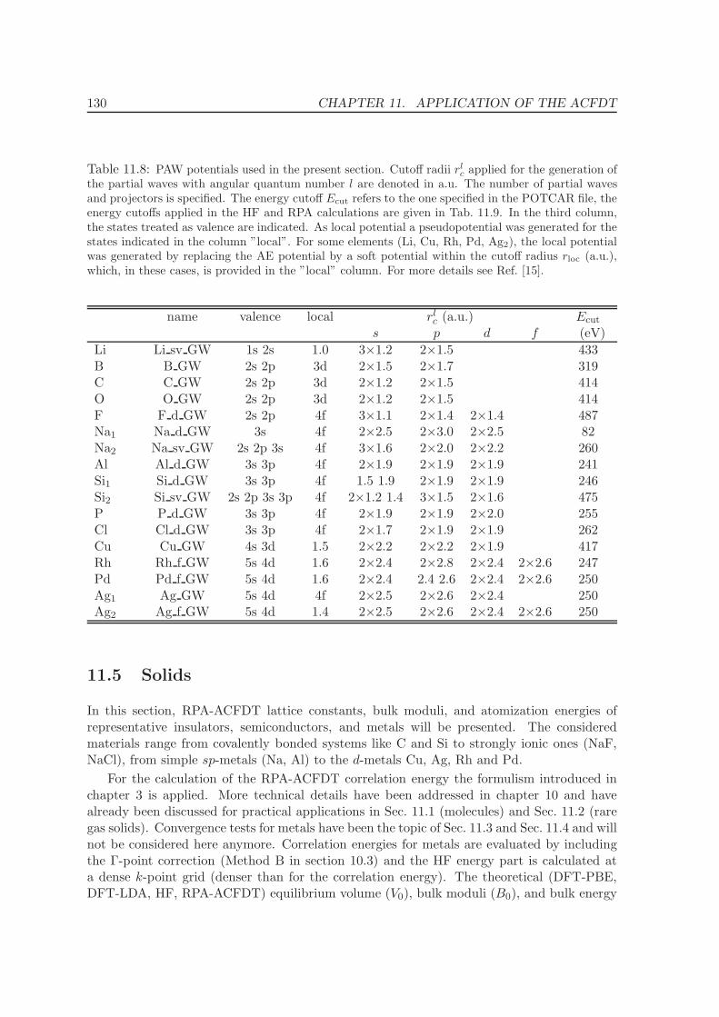
130 CHAPTER 11. APPLICATION OF THE ACFDT
Table 11.8: PAW potentials used in the present section. Cutoff radii rlc applied for the generation of
the partial waves with angular quantum number l are denoted in a.u. The number of partial wavesand projectors is specified. The energy cutoff Ecut refers to the one specified in the POTCAR file, theenergy cutoffs applied in the HF and RPA calculations are given in Tab. 11.9. In the third column,the states treated as valence are indicated. As local potential a pseudopotential was generated for thestates indicated in the column ”local”. For some elements (Li, Cu, Rh, Pd, Ag2), the local potentialwas generated by replacing the AE potential by a soft potential within the cutoff radius rloc (a.u.),which, in these cases, is provided in the ”local” column. For more details see Ref. [15].
name valence local rlc (a.u.) Ecut
s p d f (eV)
Li Li sv GW 1s 2s 1.0 3×1.2 2×1.5 433B B GW 2s 2p 3d 2×1.5 2×1.7 319C C GW 2s 2p 3d 2×1.2 2×1.5 414O O GW 2s 2p 3d 2×1.2 2×1.5 414F F d GW 2s 2p 4f 3×1.1 2×1.4 2×1.4 487Na1 Na d GW 3s 4f 2×2.5 2×3.0 2×2.5 82Na2 Na sv GW 2s 2p 3s 4f 3×1.6 2×2.0 2×2.2 260Al Al d GW 3s 3p 4f 2×1.9 2×1.9 2×1.9 241Si1 Si d GW 3s 3p 4f 1.5 1.9 2×1.9 2×1.9 246Si2 Si sv GW 2s 2p 3s 3p 4f 2×1.2 1.4 3×1.5 2×1.6 475P P d GW 3s 3p 4f 2×1.9 2×1.9 2×2.0 255Cl Cl d GW 3s 3p 4f 2×1.7 2×1.9 2×1.9 262Cu Cu GW 4s 3d 1.5 2×2.2 2×2.2 2×1.9 417Rh Rh f GW 5s 4d 1.6 2×2.4 2×2.8 2×2.4 2×2.6 247Pd Pd f GW 5s 4d 1.6 2×2.4 2.4 2.6 2×2.4 2×2.6 250Ag1 Ag GW 5s 4d 4f 2×2.5 2×2.6 2×2.4 250Ag2 Ag f GW 5s 4d 1.4 2×2.5 2×2.6 2×2.4 2×2.6 250
11.5 Solids
In this section, RPA-ACFDT lattice constants, bulk moduli, and atomization energies ofrepresentative insulators, semiconductors, and metals will be presented. The consideredmaterials range from covalently bonded systems like C and Si to strongly ionic ones (NaF,NaCl), from simple sp-metals (Na, Al) to the d-metals Cu, Ag, Rh and Pd.
For the calculation of the RPA-ACFDT correlation energy the formulism introduced inchapter 3 is applied. More technical details have been addressed in chapter 10 and havealready been discussed for practical applications in Sec. 11.1 (molecules) and Sec. 11.2 (raregas solids). Convergence tests for metals have been the topic of Sec. 11.3 and Sec. 11.4 and willnot be considered here anymore. Correlation energies for metals are evaluated by includingthe Γ-point correction (Method B in section 10.3) and the HF energy part is calculated ata dense k-point grid (denser than for the correlation energy). The theoretical (DFT-PBE,DFT-LDA, HF, RPA-ACFDT) equilibrium volume (V0), bulk moduli (B0), and bulk energy
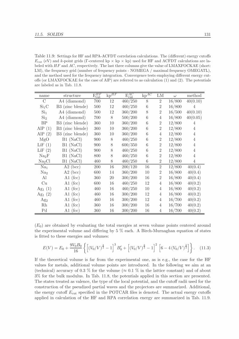
11.5. SOLIDS 131
Table 11.9: Settings for HF and RPA-ACFDT correlation calculations. The (different) energy cutoffsEcut (eV) and k-point grids (Γ-centered kp × kp × kp) used for HF and ACFDT calculations are la-beled withHF and AC, respectively. The last three columns give the value of LMAXFOCKAE (short:LM), the frequency grid (number of frequency points - NOMEGA / maximal frequency OMEGATL),and the method used for the frequency integration. Convergence tests employing different energy cut-offs (or LMAXFOCKAE for the case of AlP) are referred to as calculation (1) and (2). The potentialsare labeled as in Tab. 11.8.
name structure EHFcut kpHF EAC
cut kpAC LM ω method
C A4 (diamond) 700 12 460/250 8 2 16/800 40(0.10)Si1C B3 (zinc blende) 500 12 460/250 6 2 16/800 4Si1 A4 (diamond) 500 12 360/200 8 2 16/500 40(0.10)Si2 A4 (diamond) 700 8 500/200 6 4 16/800 40(0.05)BP B3 (zinc blende) 360 10 360/200 6 2 12/800 4
AlP (1) B3 (zinc blende) 360 10 360/200 6 2 12/800 4AlP (2) B3 (zinc blende) 360 10 360/200 6 4 12/800 4MgO B1 (NaCl) 900 8 460/250 6 2 12/800 4
LiF (1) B1 (NaCl) 900 8 600/350 6 2 12/800 4LiF (2) B1 (NaCl) 900 8 460/250 6 2 12/800 4Na2F B1 (NaCl) 800 8 460/250 6 2 12/800 4Na2Cl B1 (NaCl) 460 8 460/250 6 2 12/800 4
Na1 A2 (bcc) 200 16 200/120 16 2 12/800 40(0.4)Na2 A2 (bcc) 600 14 360/200 10 2 16/800 40(0.4)Al A1 (fcc) 360 20 300/200 16 2 16/800 40(0.4)Cu A1 (fcc) 600 16 460/250 12 4 16/800 40(0.2)
Ag1 (1) A1 (fcc) 460 16 460/250 10 4 16/800 40(0.2)Ag1 (2) A1 (fcc) 460 16 300/200 12 4 16/800 40(0.2)
Ag2 A1 (fcc) 460 16 300/200 12 4 16/700 40(0.2)Rh A1 (fcc) 360 16 300/200 16 4 16/700 40(0.2)Pd A1 (fcc) 360 16 300/200 16 4 16/700 40(0.2)
(E0) are obtained by evaluating the total energies at seven volume points centered aroundthe experimental volume and differing by 5 % each. A Birch-Murnaghan equation of statesis fitted to these energies and volumes:
E(V ) = E0 +9V0B0
16
[(V0/V )
23 − 1
]3B′
0 +[(V0/V )
23 − 1
]2 [6− 4 (V0/V )
23
]. (11.3)
If the theoretical volume is far from the experimental one, as is e.g., the case for the HFvalues for metals, additional volume points are introduced. In the following we aim at an(technical) accuracy of 0.3 % for the volume (≈ 0.1 % in the lattice constant) and of about3% for the bulk modulus. In Tab. 11.8, the potentials applied in this section are presented.The states treated as valence, the type of the local potential, and the cutoff radii used for theconstruction of the pseudized partial waves and the projectors are summarized. Additional,the energy cutoff Ecut specified in the POTCAR files is denoted. The actual energy cutoffsapplied in calculation of the HF and RPA correlation energy are summarized in Tab. 11.9.
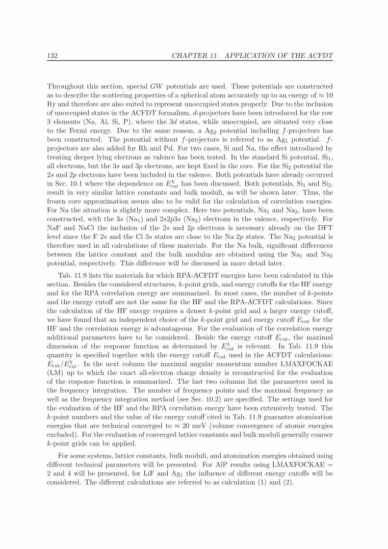
132 CHAPTER 11. APPLICATION OF THE ACFDT
Throughout this section, special GW potentials are used. These potentials are constructedas to describe the scattering properties of a spherical atom accurately up to an energy of ≈ 10Ry and therefore are also suited to represent unoccupied states properly. Due to the inclusionof unoccupied states in the ACFDT formalism, d-projectors have been introduced for the row3 elements (Na, Al, Si, P), where the 3d states, while unoccupied, are situated very closeto the Fermi energy. Due to the same reason, a Ag2 potential including f -projectors hasbeen constructed. The potential without f -projectors is referred to as Ag1 potential. f -projectors are also added for Rh and Pd. For two cases, Si and Na, the effect introduced bytreating deeper lying electrons as valence has been tested. In the standard Si potential, Si1,all electrons, but the 3s and 3p electrons, are kept fixed in the core. For the Si2 potential the2s and 2p electrons have been included in the valence. Both potentials have already occurredin Sec. 10.1 where the dependence on Eχ
cut has been discussed. Both potentials, Si1 and Si2,result in very similar lattice constants and bulk moduli, as will be shown later. Thus, thefrozen core approximation seems also to be valid for the calculation of correlation energies.For Na the situation is slightly more complex. Here two potentials, Na1 and Na2, have beenconstructed, with the 3s (Na1) and 2s2p3s (Na2) electrons in the valence, respectively. ForNaF and NaCl the inclusion of the 2s and 2p electrons is necessary already on the DFTlevel since the F 2s and the Cl 3s states are close to the Na 2p states. The Na2 potential istherefore used in all calculations of these materials. For the Na bulk, significant differencesbetween the lattice constant and the bulk modulus are obtained using the Na1 and Na2
potential, respectively. This difference will be discussed in more detail later.
Tab. 11.9 lists the materials for which RPA-ACFDT energies have been calculated in thissection. Besides the considered structures, k-point grids, and energy cutoffs for the HF energyand for the RPA correlation energy are summarized. In most cases, the number of k-pointsand the energy cutoff are not the same for the HF and the RPA-ACFDT calculations. Sincethe calculation of the HF energy requires a denser k-point grid and a larger energy cutoff,we have found that an independent choice of the k-point grid and energy cutoff Ecut for theHF and the correlation energy is advantageous. For the evaluation of the correlation energyadditional parameters have to be considered. Beside the energy cutoff Ecut, the maximaldimension of the response function as determined by Eχ
cut is relevant. In Tab. 11.9 thisquantity is specified together with the energy cutoff Ecut used in the ACFDT calculations:Ecut/E
χcut. In the next column the maximal angular momentum number LMAXFOCKAE
(LM) up to which the exact all-electron charge density is reconstructed for the evaluationof the response function is summarized. The last two columns list the parameters used inthe frequency integration. The number of frequency points and the maximal frequency aswell as the frequency integration method (see Sec. 10.2) are specified. The settings used forthe evaluation of the HF and the RPA correlation energy have been extensively tested. Thek-point numbers and the value of the energy cutoff cited in Tab. 11.9 guarantee atomizationenergies that are technical converged to ≈ 20 meV (volume convergence of atomic energiesexcluded). For the evaluation of converged lattice constants and bulk moduli generally coarserk-point grids can be applied.
For some systems, lattice constants, bulk moduli, and atomization energies obtained usingdifferent technical parameters will be presented. For AlP results using LMAXFOCKAE =2 and 4 will be presented, for LiF and Ag1 the influence of different energy cutoffs will beconsidered. The different calculations are referred to as calculation (1) and (2).
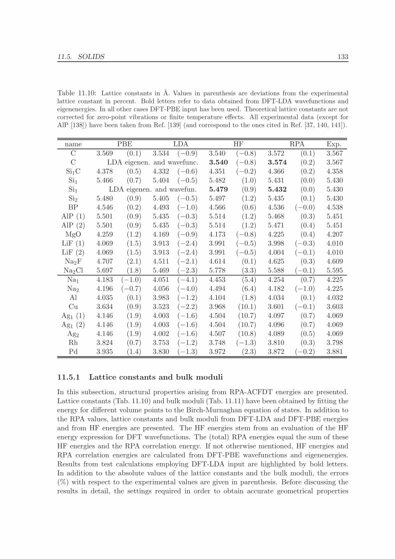
11.5. SOLIDS 133
Table 11.10: Lattice constants in A. Values in parenthesis are deviations from the experimentallattice constant in percent. Bold letters refer to data obtained from DFT-LDA wavefunctions andeigenenergies. In all other cases DFT-PBE input has been used. Theoretical lattice constants are notcorrected for zero-point vibrations or finite temperature effects. All experimental data (except forAlP [138]) have been taken from Ref. [139] (and correspond to the ones cited in Ref. [37, 140, 141]).
name PBE LDA HF RPA Exp.
C 3.569 (0.1) 3.534 (−0.9) 3.540 (−0.8) 3.572 (0.1) 3.567C LDA eigenen. and wavefunc. 3.540 (−0.8) 3.574 (0.2) 3.567
Si1C 4.378 (0.5) 4.332 (−0.6) 4.351 (−0.2) 4.366 (0.2) 4.358Si1 5.466 (0.7) 5.404 (−0.5) 5.482 (1.0) 5.431 (0.0) 5.430Si1 LDA eigenen. and wavefun. 5.479 (0.9) 5.432 (0.0) 5.430Si2 5.480 (0.9) 5.405 (−0.5) 5.497 (1.2) 5.435 (0.1) 5.430BP 4.546 (0.2) 4.493 (−1.0) 4.566 (0.6) 4.536 (−0.0) 4.538
AlP (1) 5.501 (0.9) 5.435 (−0.3) 5.514 (1.2) 5.468 (0.3) 5.451AlP (2) 5.501 (0.9) 5.435 (−0.3) 5.514 (1.2) 5.471 (0.4) 5.451MgO 4.259 (1.2) 4.169 (−0.9) 4.173 (−0.8) 4.225 (0.4) 4.207
LiF (1) 4.069 (1.5) 3.913 (−2.4) 3.991 (−0.5) 3.998 (−0.3) 4.010LiF (2) 4.069 (1.5) 3.913 (−2.4) 3.991 (−0.5) 4.004 (−0.1) 4.010Na2F 4.707 (2.1) 4.511 (−2.1) 4.614 (0.1) 4.625 (0.3) 4.609Na2Cl 5.697 (1.8) 5.469 (−2.3) 5.778 (3.3) 5.588 (−0.1) 5.595
Na1 4.183 (−1.0) 4.051 (−4.1) 4.453 (5.4) 4.254 (0.7) 4.225Na2 4.196 (−0.7) 4.056 (−4.0) 4.494 (6.4) 4.182 (−1.0) 4.225Al 4.035 (0.1) 3.983 (−1.2) 4.104 (1.8) 4.034 (0.1) 4.032Cu 3.634 (0.9) 3.523 (−2.2) 3.968 (10.1) 3.601 (−0.1) 3.603
Ag1 (1) 4.146 (1.9) 4.003 (−1.6) 4.504 (10.7) 4.097 (0.7) 4.069Ag1 (2) 4.146 (1.9) 4.003 (−1.6) 4.504 (10.7) 4.096 (0.7) 4.069
Ag2 4.146 (1.9) 4.002 (−1.6) 4.507 (10.8) 4.089 (0.5) 4.069Rh 3.824 (0.7) 3.753 (−1.2) 3.748 (−1.3) 3.810 (0.3) 3.798Pd 3.935 (1.4) 3.830 (−1.3) 3.972 (2.3) 3.872 (−0.2) 3.881
11.5.1 Lattice constants and bulk moduli
In this subsection, structural properties arising from RPA-ACFDT energies are presented.Lattice constants (Tab. 11.10) and bulk moduli (Tab. 11.11) have been obtained by fitting theenergy for different volume points to the Birch-Murnaghan equation of states. In addition tothe RPA values, lattice constants and bulk moduli from DFT-LDA and DFT-PBE energiesand from HF energies are presented. The HF energies stem from an evaluation of the HFenergy expression for DFT wavefunctions. The (total) RPA energies equal the sum of theseHF energies and the RPA correlation energy. If not otherwise mentioned, HF energies andRPA correlation energies are calculated from DFT-PBE wavefunctions and eigenenergies.Results from test calculations employing DFT-LDA input are highlighted by bold letters.In addition to the absolute values of the lattice constants and the bulk moduli, the errors(%) with respect to the experimental values are given in parenthesis. Before discussing theresults in detail, the settings required in order to obtain accurate geometrical properties
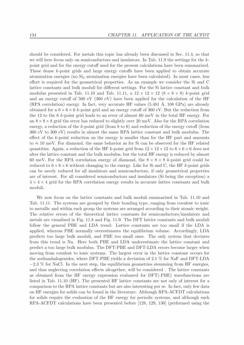
134 CHAPTER 11. APPLICATION OF THE ACFDT
should be considered. For metals this topic has already been discussed in Sec. 11.4, so thatwe will here focus only on semiconductors and insulators. In Tab. 11.9 the settings for the k-point grid and for the energy cutoff used for the present calculations have been summarized.These dense k-point grids and large energy cutoffs have been applied to obtain accurateatomization energies (no Si2 atomization energies have been calculated). In most cases, lesseffort is required for the geometrical properties. As an example we consider the Si and Clattice constants and bulk moduli for different settings. For the Si lattice constant and bulkmodulus presented in Tab. 11.10 and Tab. 11.11, a 12 × 12 × 12 (8 × 8 × 8) k-point gridand an energy cutoff of 500 eV (360 eV) have been applied for the calculation of the HF(RPA correlation) energy. In fact, very accurate HF values (5.481 A, 108 GPa) are alreadyobtained for a 6× 6× 6 k-point grid and an energy cutoff of 360 eV. But the reduction fromthe 12 to the 6 k-point grid leads to an error of almost 60 meV in the total HF energy. Foran 8× 8× 8 grid the error has reduced to slightly over 20 meV. Also for the RPA correlationenergy, a reduction of the k-point grid (from 8 to 6) and reduction of the energy cutoff (from360 eV to 300 eV) results in almost the same RPA lattice constant and bulk modulus. Theeffect of the k-point reduction on the energy is smaller than for the HF part and amountsto ≈ 10 meV. For diamond, the same behavior as for Si can be observed for the HF relatedquantities. Again, a reduction of the HF k-point grid from 12× 12× 12 to 6× 6× 6 does notalter the lattice constant and the bulk modulus, but the total HF energy is reduced by almost60 meV. For the RPA correlation energy of diamond, the 8 × 8 × 8 k-point grid could bereduced to 6× 6× 6 without changing to the energy. Like for Si and C, the HF k-point gridscan be savely reduced for all insulators and semiconductors, if only geometrical propertiesare of interest. For all considered semiconductors and insulators (Si being the exception) a4 × 4× 4 grid for the RPA correlation energy results in accurate lattice constants and bulkmoduli.
We now focus on the lattice constants and bulk moduli summarized in Tab. 11.10 andTab. 11.11. The systems are grouped by their bonding type, ranging from covalent to ionicto metallic and within each group the systems are arranged according to their atomic weight.The relative errors of the theoretical lattice constants for semiconductors/insulators andmetals are visualized in Fig. 11.8 and Fig. 11.9. The DFT lattice constants and bulk modulifollow the general PBE and LDA trend: Lattice constants are too small if the LDA isapplied, whereas PBE normally overestimates the equilibrium volume. Accordingly, LDApredicts too large bulk moduli, and PBE too small ones. The only system that deviatesfrom this trend is Na. Here both PBE and LDA underestimate the lattice constant andpredict a too large bulk modulus. The DFT-PBE and DFT-LDA errors become larger whenmoving from covalent to ionic systems. The largest error in the lattice constant occurs forthe sodiumhalogenides, where DFT-PBE yields a deviation of 2.1 % for NaF and DFT-LDA−2.3 % for NaCl. In the next step, the equilibrium geometries stemming from HF energies,and thus neglecting correlation effects altogether, will be considered . The lattice constantsas obtained from the HF energy expression evaluated for DFT(-PBE) wavefunctions arelisted in Tab. 11.10 (HF). The presented HF lattice constants are not only of interest for acomparison to the RPA lattice constants but are also interesting per se. In fact, only few dataon HF energies for solids can be found in the literature. Although RPA-ACFDT calculationsfor solids require the evaluation of the HF energy for periodic systems, and although suchRPA-ACFDT calculations have been presented before [128, 129, 130] (performed using the
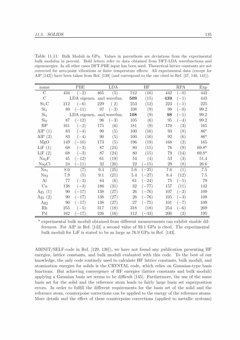
11.5. SOLIDS 135
Table 11.11: Bulk Moduli in GPa. Values in parenthesis are deviations from the experimentalbulk modulus in percent. Bold letters refer to data obtained from DFT-LDA wavefunctions andeigenenergies. In all other cases DFT-PBE input has been used. Theoretical lattice constants are notcorrected for zero-point vibrations or finite temperature effects. All experimental data (except forAlP [142]) have been taken from Ref. [139] (and correspond to the one cited in Ref. [37, 140, 141]).
name PBE LDA HF RPA Exp
C 434 (−2) 465 (5) 512 (16) 442 (−0) 443C LDA eigenen. and wavefun. 509 (15) 439 (−1) 443
Si1C 212 (−6) 229 ( 2) 253 (12) 223 (−1) 225Si1 89 (−11) 97 (−3) 108 (9) 99 (−0) 99.2Si1 LDA eigenen. and wavefun. 108 (9) 98 (−1) 99.2Si2 87 (−12) 96 (−3) 105 (6) 95 (−4) 99.2BP 161 (−2) 175 (6) 181 (9) 170 (3) 165
AlP (1) 83 (−4) 90 (5) 100 (16) 93 (8) 86a
AlP (2) 83 (−4) 90 (5) 100 (16) 92 (6) 86a
MgO 149 (−10) 173 (5) 196 (19) 168 (2) 165LiF (1) 68 (−3) 87 (24) 80 (15) 76 (9) 69.8a
LiF (2) 68 (−3) 87 (24) 80 (15) 79 (14) 69.8a
Na2F 45 (−12) 61 (19) 54 (4) 53 (3) 51.4Na2Cl 24 (−11) 32 (20) 22 (−15) 29 (8) 26.6
Na1 8.0 (7) 9.4 (25) 5.6 (−25) 7.6 (1) 7.5Na2 7.9 (5) 9.1 (21) 5.4 (−27) 8.4 (12) 7.5Al 77 (−3) 84 (6) 61 (−24) 75 (−5) 79Cu 138 (−3) 186 (31) 32 (−77) 157 (11) 142
Ag1 (1) 90 (−17) 138 (27) 26 (−76) 107 (−2) 109Ag1 (2) 90 (−17) 138 (27) 26 (−76) 105 (−3) 109
Ag2 90 (−17) 138 (27) 27 (−75) 101 (−7) 109Rh 255 (−5) 317 (18) 318 (18) 254 (−6) 269Pd 162 (−17) 226 (16) 112 (−43) 200 (3) 195
a experimental bulk moduli obtained from different measurements can exhibit sizable dif-ferences. For AlP in Ref. [142] a second value of 93.1 GPa is cited. The experimentalbulk moduli for LiF is stated to be as large as 76.9 GPa in Ref. [143].
ABINIT/SELF-code in Ref. [129, 130]), we have not found any publication presenting HFenergies, lattice constants, and bulk moduli evaluated with this code. To the best of ourknowledge, the only code routinely used to calculate HF lattice constants, bulk moduli, andatomization energies for solids is the CRYSTAL code, which relies on Gaussian-type basisfunctions. But achieving convergence of HF energies (lattice constants and bulk moduli)applying a Gaussian basis set seems to be difficult [145]. Furthermore, the use of the samebasis set for the solid and the reference atom leads to fairly large basis set superpositionerrors. In order to fulfill the different requirements for the basis set of the solid and thereference atom, counterpoise corrections can be applied to the energy of the reference atoms.More details and the effect of these counterpoise corrections (applied to metallic systems)
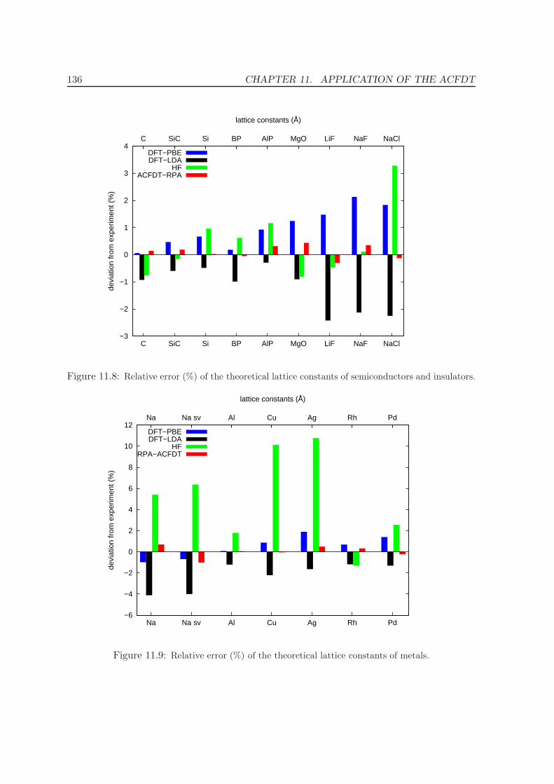
136 CHAPTER 11. APPLICATION OF THE ACFDT
−3
−2
−1
0
1
2
3
4
NaClNaFLiFMgOAlPBPSiSiCC
NaClNaFLiFMgOAlPBPSiSiCC
devi
atio
n fr
om e
xper
imen
t (%
)lattice constants (Å)
DFT−PBEDFT−LDA
HF ACFDT−RPA
Figure 11.8: Relative error (%) of the theoretical lattice constants of semiconductors and insulators.
−6
−4
−2
0
2
4
6
8
10
12
Na sv Al Cu AgNa Rh Pd
Na sv Al Cu AgNa Rh Pd
devi
atio
n fr
om e
xper
imen
t (%
)
lattice constants (Å)
DFT−PBEDFT−LDA
HFRPA−ACFDT
Figure 11.9: Relative error (%) of the theoretical lattice constants of metals.
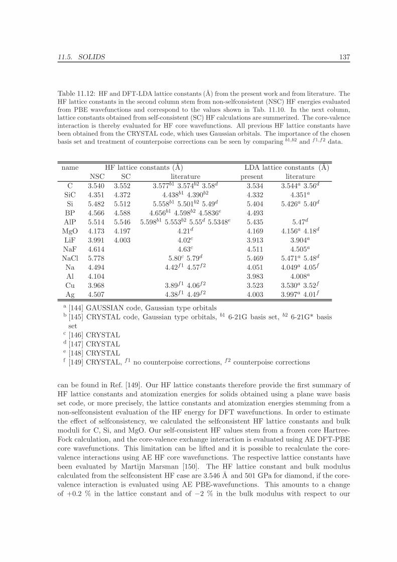
11.5. SOLIDS 137
Table 11.12: HF and DFT-LDA lattice constants (A) from the present work and from literature. TheHF lattice constants in the second column stem from non-selfconsistent (NSC) HF energies evaluatedfrom PBE wavefunctions and correspond to the values shown in Tab. 11.10. In the next column,lattice constants obtained from self-consistent (SC) HF calculations are summerized. The core-valenceinteraction is thereby evaluated for HF core wavefunctions. All previous HF lattice constants havebeen obtained from the CRYSTAL code, which uses Gaussian orbitals. The importance of the chosenbasis set and treatment of counterpoise corrections can be seen by comparing b1,b2 and f1,f2 data.
name HF lattice constants (A) LDA lattice constants (A)NSC SC literature present literature
C 3.540 3.552 3.577b1 3.574b2 3.58d 3.534 3.544a 3.56d
SiC 4.351 4.372 4.438b1 4.390b2 4.332 4.351a
Si 5.482 5.512 5.558b1 5.501b2 5.49d 5.404 5.426a 5.40d
BP 4.566 4.588 4.656b1 4.598b2 4.5836e 4.493AlP 5.514 5.546 5.598b1 5.553b2 5.55d 5.5348e 5.435 5.47d
MgO 4.173 4.197 4.21d 4.169 4.156a 4.18d
LiF 3.991 4.003 4.02c 3.913 3.904a
NaF 4.614 4.63c 4.511 4.505a
NaCl 5.778 5.80c 5.79d 5.469 5.471a 5.48d
Na 4.494 4.42f1 4.57f2 4.051 4.049a 4.05f
Al 4.104 3.983 4.008a
Cu 3.968 3.89f1 4.06f2 3.523 3.530a 3.52f
Ag 4.507 4.38f1 4.49f2 4.003 3.997a 4.01f
a [144] GAUSSIAN code, Gaussian type orbitalsb [145] CRYSTAL code, Gaussian type orbitals, b1 6-21G basis set, b2 6-21G* basis
setc [146] CRYSTALd [147] CRYSTALe [148] CRYSTALf [149] CRYSTAL, f1 no counterpoise corrections, f2 counterpoise corrections
can be found in Ref. [149]. Our HF lattice constants therefore provide the first summary ofHF lattice constants and atomization energies for solids obtained using a plane wave basisset code, or more precisely, the lattice constants and atomization energies stemming from anon-selfconsistent evaluation of the HF energy for DFT wavefunctions. In order to estimatethe effect of selfconsistency, we calculated the selfconsistent HF lattice constants and bulkmoduli for C, Si, and MgO. Our self-consistent HF values stem from a frozen core Hartree-Fock calculation, and the core-valence exchange interaction is evaluated using AE DFT-PBEcore wavefunctions. This limitation can be lifted and it is possible to recalculate the core-valence interactions using AE HF core wavefunctions. The respective lattice constants havebeen evaluated by Martijn Marsman [150]. The HF lattice constant and bulk moduluscalculated from the selfconsistent HF case are 3.546 A and 501 GPa for diamond, if the core-valence interaction is evaluated using AE PBE-wavefunctions. This amounts to a changeof +0.2 % in the lattice constant and of −2 % in the bulk modulus with respect to our
138 CHAPTER 11. APPLICATION OF THE ACFDT
non-selfconsistent HF values. If the core states stem from a HF reference calculation, theselfconsistent HF lattice constant further increases to 3.552 A (+0.3 % compared to the non-selfconsistend HF value). For Si and MgO, the selfconsistent HF lattice constants become5.493 A (+0.2 %) and 4.187 A (+0.3%), the bulk moduli 105 GPa (−3 %) and 185 GPa(−6 %), if the core-valence interaction is recalculated using PBE core wavefunctions. UsingHF core wavefunctions enhances the difference, and the selfconsistent HF lattice constantsbecome 5.512 A (+0.5 %) and 4.197 A (+0.6%) for Si and MgO, respectively. Also for theother considered materials, selfconsistency leads to an increase of the HF lattice constant(see Tab. 11.12). If the core-valence interaction is recalculated using HF core wavefunctions,the corresponding lattice constants are 0.3 % to 0.6 % larger than the values stemmingfrom non-selfconsistent HF calculations based on PBE wavefunctions. In Tab. 11.12, our HFlattice constants are compared to values obtained using the CRYSTAL code. In addition,selfconsistent HF lattice constants recalculating the core-valence interaction with HF corewavefunctions as evaluated by Martijn Marsman are presented. Even on the level of DFT-LDA, lattice constants obtained using a local and a plane wave basis set can differ by ≈ 0.4%. For most considered systems, the plane wave LDA lattice constants are smaller than theones evaluated using Gaussian type orbitals. It is evident that HF lattice constants evaluatedusing CRYSTAL show large deviations for different basis sets applied. In Ref. [145], latticeconstants have been calculated for C, SiC, Si, BP, and AlP using the CRYSTAL code. Theresults, labeled with b1 and b2 in Tab. 11.12, have been obtained for two different local basissets, 6-21G and 6-21G*, where the latter includes polarization functions. For SiC, Si, BP,and AlP, the difference between the HF lattice constants obtained from the 6-21G and 6-21G* basis set amounts to ≈ 1%. If we take the 6-21G* lattice constant as a reference, thedifference between our self-consistent lattice constants and the CRYSTAL values is 0.6 %for diamond and <0.4 % for the other materials, which is smaller than the error observedfor different local basis sets. For metallic systems, the basis set superposition error plays animportant role. The inclusion of counterpoise corrections leads to a change of up to 4 % (Cu)in the lattice constant. The difference between the counterpoise corrected lattice constantsfrom Ref. [145] and our (non-selfconsistent) HF values is 1.5 % for Na, 2.3 % for Cu, and−0.4 % for Ag.
For semiconductors and insulators (see Fig. 11.8), the HF lattice constants (errors ingreen) are not worse than DFT-LDA (black) and DFT-PBE (blue). As a general trend,too small lattice constants are obtained for the lighter systems and too large ones for solidsformed of heavier atoms. An illustrative example are the alkali halides LiF, NaF, and NaClwhere the error in the lattice constant increases from −0.5 to 0.1 to 3.3 %. The same trendas observed in the present work was also found by Prencipe and coworkers [147] (see valuesin Tab. 11.12), who performed HF calculations for alkali halides. They ascribed the increasein the HF lattice constant when going from F to Cl to two effects: first, due to the lack ofcorrelation, the HF ions are too large. Secondly, dispersion forces (which are neglected if onlythe HF contribution is considered) are proportional to the polarization of the atoms and thepolarization is again larger for heavier atoms. The neglect of the attractive polarization effectstherefore leads to an increase of the lattice constant with the atomic mass. For the presentlyconsidered semiconductors and insulators the HF bulk moduli are normally too large. Theonly exception from this trend is NaCl, where the bulk modulus is underestimated by −15%.
11.5. SOLIDS 139
Almost all HF lattice constants (bulk moduli) presented in Tab. 11.10 (Tab. 11.11) havebeen evaluated on top of DFT-PBE wavefunctions. Only for C and Si, values resulting fromDFT-LDA input are shown as well (bold numbers). The effect of the different exchange-correlation potential is very small. Another test concerns the effect introduced if deeperlying states are included in the valence. For two materials, Si and Na, such potentials havebeen generated and are referred to as Si2 and Na2. For Si, the effect resulting from theincreased number of valence electrons amounts to a change of +0.3 % in the lattice constant.For Na, the difference in the lattice constant related to the use of either the Na1 or Na2
potential is with an 1.0 % change significantly larger. The magnitude of this change is toolarge to be related to an insufficient k-point grid or energy cutoff, it has to be related to thechoice of the potentials. One reason why the inclusion of 2s and 2p electrons results in largerdeviations for Na than for Si can be found in the energetic vicinity of these states to theouter shell states for the case of Na. While the 2s and 2p states are situated −133 eV and−90 eV below the Fermi energy for Si, they are only −53 eV and −25 eV below the Fermienergy for Na. Thus the inclusion of these states is more important for the description ofNa. In Fig. 11.10 and Fig. 11.11 the HF energy for Si and Na, respectively, are shown onthe left hand side. We will return to the inclusion of deeper lying states when discussing theinfluence of the RPA correlation energy on the equilibrium volume of Si and Na.
In contrast to the case of semiconductors and insulators, where HF provides a reasonableestimate for the lattice constants and (to a lesser extend) for the bulk moduli, HF failsdramatically for the description of metals. For all considered metals, except for Rh, the HFlattice constants are too large with errors being up to ≈ 6 % for Na and 10 % for Cu andAg. The bulk moduli, which have been overestimated for almost all considered insulatorsand semiconductors, are now severely underestimated (again with the exception of Rh). Theerrors in the HF lattice constants and bulk moduli are most severe for the free-electronlike metals Na, Cu, and Ag. For Al, and especially for the transition metals Rh and Pd,where the covalent contribution to the binding is significantly stronger, HF yields closeragreement to experiment. In the case of Rh, HF even underestimates the lattice constant,and overestimates the bulk modulus.
We finally focus on the RPA lattice constants and bulk moduli (errors are given in redin Fig. 11.8 and Fig. 11.9). The inclusion of correlation effects drastically improves thegeometrical properties of the metallic systems compared to HF. For sodium, the error in thelattice constant is reduced from over 6 % to under 1 % (mind the relative large deviationsof values obtained using the Na1 and Na2 potential). For the noble metals Cu and Ag, therelative errors are −0.1 % for Cu and 0.5 % for Ag compared to a 10 % mismatch in the HFcase. A similar improvement is observed for the bulk moduli. For the semiconductors andinsulators, the quality of the RPA lattice constants is even better than for the metals, with amaximal error of 0.4 % for AlP and MgO, although the improvement compared to the alreadyrelative good HF values is not as impressive. In contrast to the DFT lattice constants, whichexhibit increasing errors when the ionic character of the material prevails, and the HF values,for which the error depends on the atomic weight, the RPA lattice constants give constantlygood results for covalent, ionic, and metallic systems and show no dependence on the weight.The RPA bulk moduli tend to exceed the experimental values. All in all, we find that theRPA provides a very good description of geometrical properties for metals, semiconductors,and insulators.
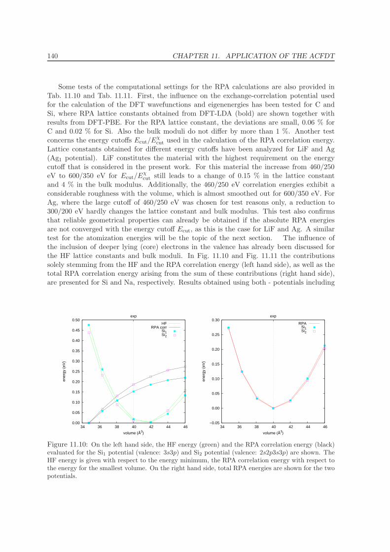
140 CHAPTER 11. APPLICATION OF THE ACFDT
Some tests of the computational settings for the RPA calculations are also provided inTab. 11.10 and Tab. 11.11. First, the influence on the exchange-correlation potential usedfor the calculation of the DFT wavefunctions and eigenenergies has been tested for C andSi, where RPA lattice constants obtained from DFT-LDA (bold) are shown together withresults from DFT-PBE. For the RPA lattice constant, the deviations are small, 0.06 % forC and 0.02 % for Si. Also the bulk moduli do not differ by more than 1 %. Another testconcerns the energy cutoffs Ecut/E
χcut used in the calculation of the RPA correlation energy.
Lattice constants obtained for different energy cutoffs have been analyzed for LiF and Ag(Ag1 potential). LiF constitutes the material with the highest requirement on the energycutoff that is considered in the present work. For this material the increase from 460/250eV to 600/350 eV for Ecut/E
χcut still leads to a change of 0.15 % in the lattice constant
and 4 % in the bulk modulus. Additionally, the 460/250 eV correlation energies exhibit aconsiderable roughness with the volume, which is almost smoothed out for 600/350 eV. ForAg, where the large cutoff of 460/250 eV was chosen for test reasons only, a reduction to300/200 eV hardly changes the lattice constant and bulk modulus. This test also confirmsthat reliable geometrical properties can already be obtained if the absolute RPA energiesare not converged with the energy cutoff Ecut, as this is the case for LiF and Ag. A similartest for the atomization energies will be the topic of the next section. The influence ofthe inclusion of deeper lying (core) electrons in the valence has already been discussed forthe HF lattice constants and bulk moduli. In Fig. 11.10 and Fig. 11.11 the contributionssolely stemming from the HF and the RPA correlation energy (left hand side), as well as thetotal RPA correlation energy arising from the sum of these contributions (right hand side),are presented for Si and Na, respectively. Results obtained using both - potentials including
0.00
0.05
0.10
0.15
0.20
0.25
0.30
0.35
0.40
0.45
0.50
34 36 38 40 42 44 46
exp
ener
gy (
eV)
volume (Å3)
HFRPA corr
Si1Si2
−0.05
0.00
0.05
0.10
0.15
0.20
0.25
0.30
34 36 38 40 42 44 46
exp
ener
gy (
eV)
volume (Å3)
RPASi1Si2
Figure 11.10: On the left hand side, the HF energy (green) and the RPA correlation energy (black)evaluated for the Si1 potential (valence: 3s3p) and Si2 potential (valence: 2s2p3s3p) are shown. TheHF energy is given with respect to the energy minimum, the RPA correlation energy with respect tothe energy for the smallest volume. On the right hand side, total RPA energies are shown for the twopotentials.
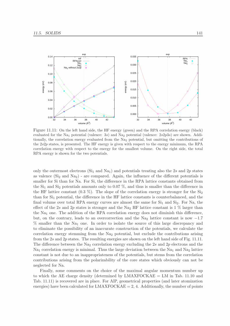
11.5. SOLIDS 141
0.00
0.02
0.04
0.06
0.08
0.10
0.12
0.14
32 34 36 38 40 42
exp
ener
gy (
eV)
volume (Å3)
HFRPAcorr
Na1Na2
Na2 without 2s2p
0.000
0.005
0.010
0.015
0.020
0.025
0.030
0.035
32 34 36 38 40 42
exp
ener
gy (
eV)
volume (Å3)
RPANa1Na2
Figure 11.11: On the left hand side, the HF energy (green) and the RPA correlation energy (black)evaluated for the Na1 potential (valence: 3s) and Na2 potential (valence: 2s2p3s) are shown. Addi-tionally, the correlation energy evaluated from the Na2 potential, but omitting the contributions ofthe 2s2p states, is presented. The HF energy is given with respect to the energy minimum, the RPAcorrelation energy with respect to the energy for the smallest volume. On the right side, the totalRPA energy is shown for the two potentials.
only the outermost electrons (Si1 and Na1) and potentials treating also the 2s and 2p statesas valence (Si2 and Na2) - are compared. Again, the influence of the different potentials issmaller for Si than for Na. For Si, the difference in the RPA lattice constants obtained fromthe Si1 and Si2 potentials amounts only to 0.07 %, and thus is smaller than the difference inthe HF lattice constant (0.3 %). The slope of the correlation energy is stronger for the Si2than for Si1 potential, the difference in the HF lattice constants is counterbalanced, and thefinal volume over total RPA energy curves are almost the same for Si1 and Si2. For Na, theeffect of the 2s and 2p states is stronger and the Na2 HF lattice constant is 1 % larger thanthe Na1 one. The addition of the RPA correlation energy does not diminish this difference,but, on the contrary, leads to an overcorrection and the Na2 lattice constant is now −1.7% smaller than the Na1 one. In order to isolate the source of this large discrepancy andto eliminate the possibility of an inaccurate construction of the potentials, we calculate thecorrelation energy stemming from the Na2 potential, but exclude the contributions arisingfrom the 2s and 2p states. The resulting energies are shown on the left hand side of Fig. 11.11.The difference between the Na2 correlation energy excluding the 2s and 2p electrons and theNa1 correlation energy is minimal. Thus the large deviation between the Na1 and Na2 latticeconstant is not due to an inappropriateness of the potentials, but stems from the correlationcontributions arising from the polarizability of the core states which obviously can not beneglected for Na.
Finally, some comments on the choice of the maximal angular momentum number upto which the AE charge density (determined by LMAXFOCKAE = LM in Tab. 11.10 andTab. 11.11) is recovered are in place. For AlP, geometrical properties (and later atomizationenergies) have been calculated for LMAXFOCKAE = 2, 4. Additionally, the number of points
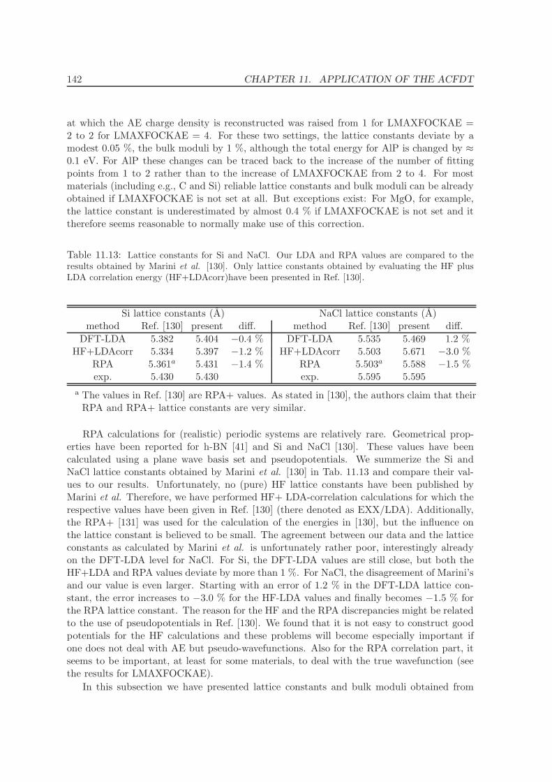
142 CHAPTER 11. APPLICATION OF THE ACFDT
at which the AE charge density is reconstructed was raised from 1 for LMAXFOCKAE =2 to 2 for LMAXFOCKAE = 4. For these two settings, the lattice constants deviate by amodest 0.05 %, the bulk moduli by 1 %, although the total energy for AlP is changed by ≈0.1 eV. For AlP these changes can be traced back to the increase of the number of fittingpoints from 1 to 2 rather than to the increase of LMAXFOCKAE from 2 to 4. For mostmaterials (including e.g., C and Si) reliable lattice constants and bulk moduli can be alreadyobtained if LMAXFOCKAE is not set at all. But exceptions exist: For MgO, for example,the lattice constant is underestimated by almost 0.4 % if LMAXFOCKAE is not set and ittherefore seems reasonable to normally make use of this correction.
Table 11.13: Lattice constants for Si and NaCl. Our LDA and RPA values are compared to theresults obtained by Marini et al. [130]. Only lattice constants obtained by evaluating the HF plusLDA correlation energy (HF+LDAcorr)have been presented in Ref. [130].
Si lattice constants (A) NaCl lattice constants (A)method Ref. [130] present diff. method Ref. [130] present diff.
DFT-LDA 5.382 5.404 −0.4 % DFT-LDA 5.535 5.469 1.2 %HF+LDAcorr 5.334 5.397 −1.2 % HF+LDAcorr 5.503 5.671 −3.0 %
RPA 5.361a 5.431 −1.4 % RPA 5.503a 5.588 −1.5 %exp. 5.430 5.430 exp. 5.595 5.595
a The values in Ref. [130] are RPA+ values. As stated in [130], the authors claim that theirRPA and RPA+ lattice constants are very similar.
RPA calculations for (realistic) periodic systems are relatively rare. Geometrical prop-erties have been reported for h-BN [41] and Si and NaCl [130]. These values have beencalculated using a plane wave basis set and pseudopotentials. We summerize the Si andNaCl lattice constants obtained by Marini et al. [130] in Tab. 11.13 and compare their val-ues to our results. Unfortunately, no (pure) HF lattice constants have been published byMarini et al. Therefore, we have performed HF+ LDA-correlation calculations for which therespective values have been given in Ref. [130] (there denoted as EXX/LDA). Additionally,the RPA+ [131] was used for the calculation of the energies in [130], but the influence onthe lattice constant is believed to be small. The agreement between our data and the latticeconstants as calculated by Marini et al. is unfortunately rather poor, interestingly alreadyon the DFT-LDA level for NaCl. For Si, the DFT-LDA values are still close, but both theHF+LDA and RPA values deviate by more than 1 %. For NaCl, the disagreement of Marini’sand our value is even larger. Starting with an error of 1.2 % in the DFT-LDA lattice con-stant, the error increases to −3.0 % for the HF-LDA values and finally becomes −1.5 % forthe RPA lattice constant. The reason for the HF and the RPA discrepancies might be relatedto the use of pseudopotentials in Ref. [130]. We found that it is not easy to construct goodpotentials for the HF calculations and these problems will become especially important ifone does not deal with AE but pseudo-wavefunctions. Also for the RPA correlation part, itseems to be important, at least for some materials, to deal with the true wavefunction (seethe results for LMAXFOCKAE).
In this subsection we have presented lattice constants and bulk moduli obtained from
11.5. SOLIDS 143
(non-selfconsistent) HF calculations and from the evaluation of the RPA correlation energy.The agreement of the HF equilibrium properties with experiment is not too bad in the caseof semiconductors and insulators, but lattice constants are vastly overestimated for metals.The RPA gives lattice constants which are drastically improved for metals, and it also yieldssatisfactory equilibrium distances for semiconductors and insulators.
11.5.2 Atomization energies
In the previous subsection, we have concentrated on the RPA equilibrium properties. Nowthe atomization energies calculated from HF and RPA energies will be considered. The at-omization energy describes the energy which is required to split a material into its fragments:
∆E = −
(Ebulk −
∑
i
Eatomi
). (11.4)
In contrast to the sign convention which we used in Sec. 11.2 for the cohesive energy, largeratomization energies mean stronger binding and vice verse.
In order to calculate the atomization energy, the energy of the isolated atom has to beevaluated. For the RPA correlation energies this step is involved, because the calculation ofthe correlation energy scales like V3 with the volume of the supercell V, and it is necessaryto use supercells with an extension of at least 8× 8× 8 A. Due to the large number of planewaves that can easily exceed 10.000 even the DFT prerun with the large number of emptybands (= number of plane waves) can become tedious. For atoms with large atomic radii,like Li and Na, Mg, and Cu and Ag, the volume convergence of both the DFT energy andthe RPA correlation energy is especially slow. Additionally, these elements are described bypotentials with high energy cutoffs, which are required because electrons from lower shells areincluded (Li, Na, Mg) or because d-electrons (Cu, Ag) are present. This further complicatesthe calculation of the correlation energy. Therefore, the correlation energies for these atomsexhibit relatively large error bars and consequently RPA atomization energies can not bespecified with an accuracy better than 50 meV for NaCl and NaF, 40 meV for LiF, and 20meV for Ag and Cu. In Tab. 11.14 atomization energies calculated using DFT-PBE, DFT-LDA, HF, and ACFDT-RPA are summarized. All atomization energies are given per atom(e.g, for AlP, energy/atom = 1/2 × energy/unit cell) and the deviation from experiment(in parenthesis) is given in eV/atom. Fig. 11.12 and Fig. 11.13 visualize these errors forsemiconductors and insulators, and for metals, respectively. Negative errors indicate thatthe method underbinds the material, positive errors indicate overbinding. The HF and RPAatomization energies all have been calculated using PBE wavefunctions. The use of the LDAwavefunctions and eigenenergies for the atomic calculations turned out to be problematic, apoint to which we will return later.
DFT-PBE describes the atomization energies well, although it does not reach chemicalaccuracy (≈ 40 meV). The error introduced by the PBE approximation can be positive (e.g.,C) or negative (e.g., Ag). The largest errors for the considered set of materials are 0.35 eVfor C and −0.43 eV for Ag, the average absolute error is 0.15 eV. The errors of the DFT-LDA atomization energies are for all considered systems larger than for DFT-PBE and a toostrong tendency towards forming a 3D solid is observed. In average, the atomization energyis by 0.76 eV (17 %) too large.
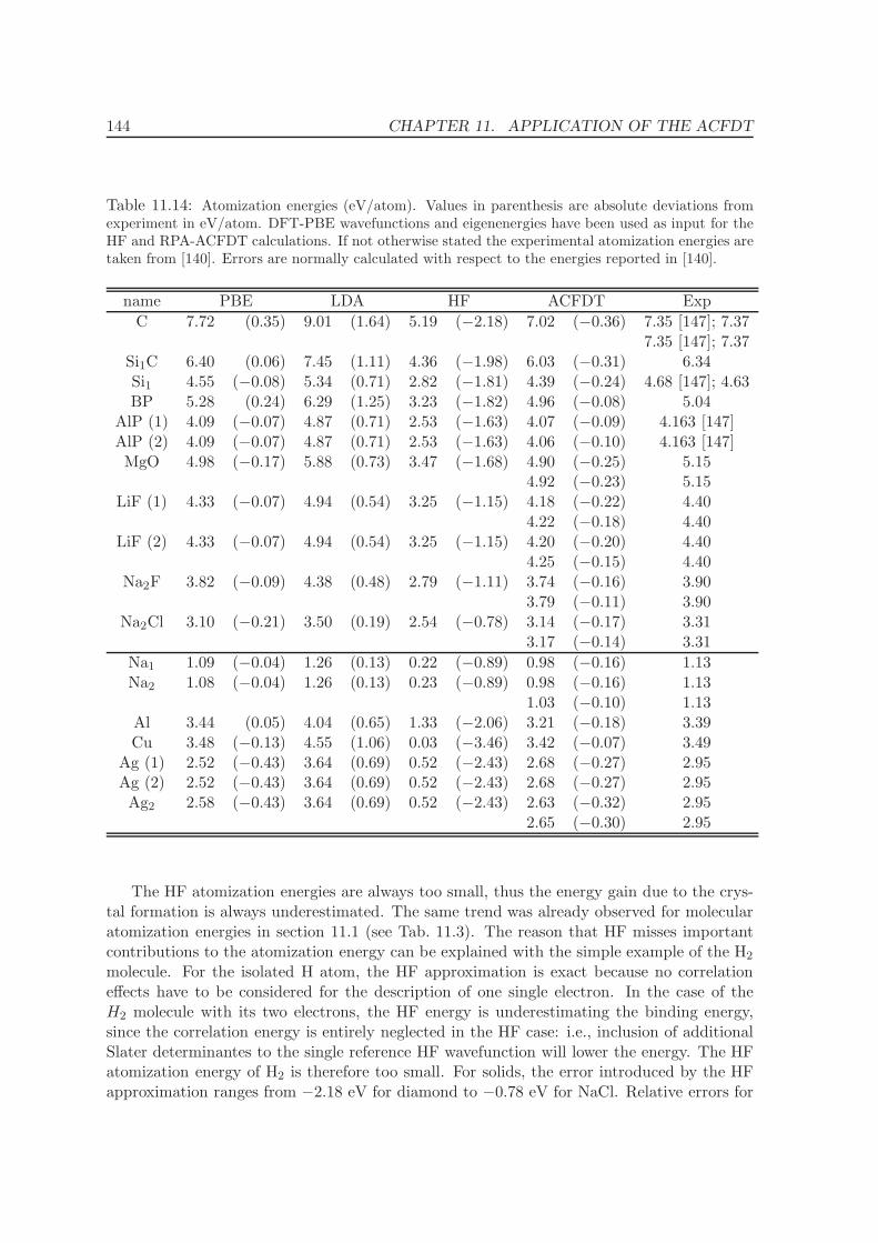
144 CHAPTER 11. APPLICATION OF THE ACFDT
Table 11.14: Atomization energies (eV/atom). Values in parenthesis are absolute deviations fromexperiment in eV/atom. DFT-PBE wavefunctions and eigenenergies have been used as input for theHF and RPA-ACFDT calculations. If not otherwise stated the experimental atomization energies aretaken from [140]. Errors are normally calculated with respect to the energies reported in [140].
name PBE LDA HF ACFDT Exp
C 7.72 (0.35) 9.01 (1.64) 5.19 (−2.18) 7.02 (−0.36) 7.35 [147]; 7.377.35 [147]; 7.37
Si1C 6.40 (0.06) 7.45 (1.11) 4.36 (−1.98) 6.03 (−0.31) 6.34Si1 4.55 (−0.08) 5.34 (0.71) 2.82 (−1.81) 4.39 (−0.24) 4.68 [147]; 4.63BP 5.28 (0.24) 6.29 (1.25) 3.23 (−1.82) 4.96 (−0.08) 5.04
AlP (1) 4.09 (−0.07) 4.87 (0.71) 2.53 (−1.63) 4.07 (−0.09) 4.163 [147]AlP (2) 4.09 (−0.07) 4.87 (0.71) 2.53 (−1.63) 4.06 (−0.10) 4.163 [147]MgO 4.98 (−0.17) 5.88 (0.73) 3.47 (−1.68) 4.90 (−0.25) 5.15
4.92 (−0.23) 5.15LiF (1) 4.33 (−0.07) 4.94 (0.54) 3.25 (−1.15) 4.18 (−0.22) 4.40
4.22 (−0.18) 4.40LiF (2) 4.33 (−0.07) 4.94 (0.54) 3.25 (−1.15) 4.20 (−0.20) 4.40
4.25 (−0.15) 4.40Na2F 3.82 (−0.09) 4.38 (0.48) 2.79 (−1.11) 3.74 (−0.16) 3.90
3.79 (−0.11) 3.90Na2Cl 3.10 (−0.21) 3.50 (0.19) 2.54 (−0.78) 3.14 (−0.17) 3.31
3.17 (−0.14) 3.31
Na1 1.09 (−0.04) 1.26 (0.13) 0.22 (−0.89) 0.98 (−0.16) 1.13Na2 1.08 (−0.04) 1.26 (0.13) 0.23 (−0.89) 0.98 (−0.16) 1.13
1.03 (−0.10) 1.13Al 3.44 (0.05) 4.04 (0.65) 1.33 (−2.06) 3.21 (−0.18) 3.39Cu 3.48 (−0.13) 4.55 (1.06) 0.03 (−3.46) 3.42 (−0.07) 3.49
Ag (1) 2.52 (−0.43) 3.64 (0.69) 0.52 (−2.43) 2.68 (−0.27) 2.95Ag (2) 2.52 (−0.43) 3.64 (0.69) 0.52 (−2.43) 2.68 (−0.27) 2.95Ag2 2.58 (−0.43) 3.64 (0.69) 0.52 (−2.43) 2.63 (−0.32) 2.95
2.65 (−0.30) 2.95
The HF atomization energies are always too small, thus the energy gain due to the crys-tal formation is always underestimated. The same trend was already observed for molecularatomization energies in section 11.1 (see Tab. 11.3). The reason that HF misses importantcontributions to the atomization energy can be explained with the simple example of the H2
molecule. For the isolated H atom, the HF approximation is exact because no correlationeffects have to be considered for the description of one single electron. In the case of theH2 molecule with its two electrons, the HF energy is underestimating the binding energy,since the correlation energy is entirely neglected in the HF case: i.e., inclusion of additionalSlater determinantes to the single reference HF wavefunction will lower the energy. The HFatomization energy of H2 is therefore too small. For solids, the error introduced by the HFapproximation ranges from −2.18 eV for diamond to −0.78 eV for NaCl. Relative errors for
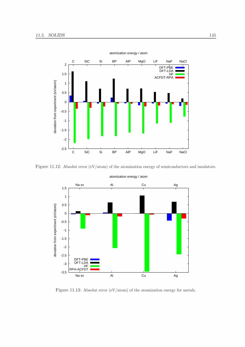
11.5. SOLIDS 145
-2.5
-2
-1.5
-1
-0.5
0
0.5
1
1.5
2
NaClNaFLiFMgOAlPBPSiSiCC
NaClNaFLiFMgOAlPBPSiSiCC
devi
atio
n fr
om e
xper
imen
t (eV
/ato
m)
atomization energy / atom
DFT-PBEDFT-LDA
HFACFDT-RPA
Figure 11.12: Absolut error (eV/atom) of the atomization energy of semiconductors and insulators.
-3.5
-3
-2.5
-2
-1.5
-1
-0.5
0
0.5
1
1.5
Na sv Al Cu Ag
Na sv Al Cu Ag
devi
atio
n fr
om e
xper
imen
t (eV
/ato
m)
atomization energy / atom
DFT-PBEDFT-LDA
HFRPA-ACFDT
Figure 11.13: Absolut error (eV/atom) of the atomization energy for metals.
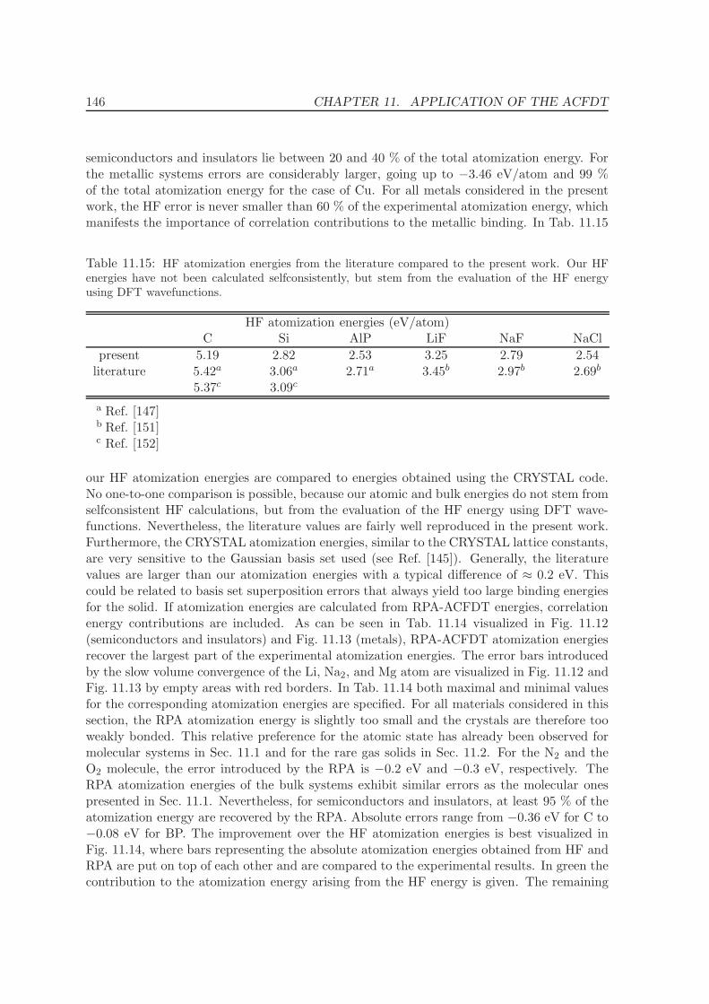
146 CHAPTER 11. APPLICATION OF THE ACFDT
semiconductors and insulators lie between 20 and 40 % of the total atomization energy. Forthe metallic systems errors are considerably larger, going up to −3.46 eV/atom and 99 %of the total atomization energy for the case of Cu. For all metals considered in the presentwork, the HF error is never smaller than 60 % of the experimental atomization energy, whichmanifests the importance of correlation contributions to the metallic binding. In Tab. 11.15
Table 11.15: HF atomization energies from the literature compared to the present work. Our HFenergies have not been calculated selfconsistently, but stem from the evaluation of the HF energyusing DFT wavefunctions.
HF atomization energies (eV/atom)C Si AlP LiF NaF NaCl
present 5.19 2.82 2.53 3.25 2.79 2.54literature 5.42a 3.06a 2.71a 3.45b 2.97b 2.69b
5.37c 3.09c
a Ref. [147]b Ref. [151]c Ref. [152]
our HF atomization energies are compared to energies obtained using the CRYSTAL code.No one-to-one comparison is possible, because our atomic and bulk energies do not stem fromselfconsistent HF calculations, but from the evaluation of the HF energy using DFT wave-functions. Nevertheless, the literature values are fairly well reproduced in the present work.Furthermore, the CRYSTAL atomization energies, similar to the CRYSTAL lattice constants,are very sensitive to the Gaussian basis set used (see Ref. [145]). Generally, the literaturevalues are larger than our atomization energies with a typical difference of ≈ 0.2 eV. Thiscould be related to basis set superposition errors that always yield too large binding energiesfor the solid. If atomization energies are calculated from RPA-ACFDT energies, correlationenergy contributions are included. As can be seen in Tab. 11.14 visualized in Fig. 11.12(semiconductors and insulators) and Fig. 11.13 (metals), RPA-ACFDT atomization energiesrecover the largest part of the experimental atomization energies. The error bars introducedby the slow volume convergence of the Li, Na2, and Mg atom are visualized in Fig. 11.12 andFig. 11.13 by empty areas with red borders. In Tab. 11.14 both maximal and minimal valuesfor the corresponding atomization energies are specified. For all materials considered in thissection, the RPA atomization energy is slightly too small and the crystals are therefore tooweakly bonded. This relative preference for the atomic state has already been observed formolecular systems in Sec. 11.1 and for the rare gas solids in Sec. 11.2. For the N2 and theO2 molecule, the error introduced by the RPA is −0.2 eV and −0.3 eV, respectively. TheRPA atomization energies of the bulk systems exhibit similar errors as the molecular onespresented in Sec. 11.1. Nevertheless, for semiconductors and insulators, at least 95 % of theatomization energy are recovered by the RPA. Absolute errors range from −0.36 eV for C to−0.08 eV for BP. The improvement over the HF atomization energies is best visualized inFig. 11.14, where bars representing the absolute atomization energies obtained from HF andRPA are put on top of each other and are compared to the experimental results. In green thecontribution to the atomization energy arising from the HF energy is given. The remaining
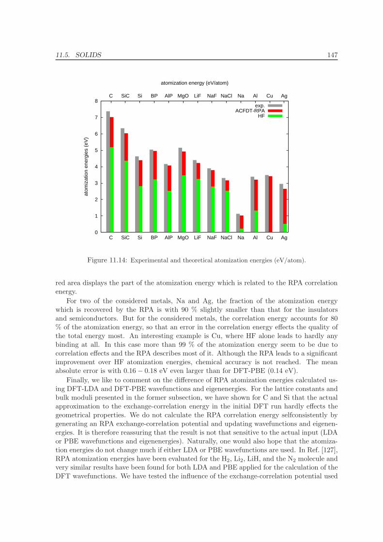
11.5. SOLIDS 147
0
1
2
3
4
5
6
7
8
AgCuAlNaNaClNaFLiFMgOAlPBPSiSiCC
AgCuAlNaNaClNaFLiFMgOAlPBPSiSiCC
atom
izat
ion
ener
gies
(eV
)atomization energy (eV/atom)
exp.ACFDT-RPA
HF
Figure 11.14: Experimental and theoretical atomization energies (eV/atom).
red area displays the part of the atomization energy which is related to the RPA correlationenergy.
For two of the considered metals, Na and Ag, the fraction of the atomization energywhich is recovered by the RPA is with 90 % slightly smaller than that for the insulatorsand semiconductors. But for the considered metals, the correlation energy accounts for 80% of the atomization energy, so that an error in the correlation energy effects the quality ofthe total energy most. An interesting example is Cu, where HF alone leads to hardly anybinding at all. In this case more than 99 % of the atomization energy seem to be due tocorrelation effects and the RPA describes most of it. Although the RPA leads to a significantimprovement over HF atomization energies, chemical accuracy is not reached. The meanabsolute error is with 0.16− 0.18 eV even larger than for DFT-PBE (0.14 eV).
Finally, we like to comment on the difference of RPA atomization energies calculated us-ing DFT-LDA and DFT-PBE wavefunctions and eigenenergies. For the lattice constants andbulk moduli presented in the former subsection, we have shown for C and Si that the actualapproximation to the exchange-correlation energy in the initial DFT run hardly effects thegeometrical properties. We do not calculate the RPA correlation energy selfconsistently bygenerating an RPA exchange-correlation potential and updating wavefunctions and eigenen-ergies. It is therefore reassuring that the result is not that sensitive to the actual input (LDAor PBE wavefunctions and eigenenergies). Naturally, one would also hope that the atomiza-tion energies do not change much if either LDA or PBE wavefunctions are used. In Ref. [127],RPA atomization energies have been evaluated for the H2, Li2, LiH, and the N2 molecule andvery similar results have been found for both LDA and PBE applied for the calculation of theDFT wavefunctions. We have tested the influence of the exchange-correlation potential used
148 CHAPTER 11. APPLICATION OF THE ACFDT
in the KS-DFT calculations on the atomization energies of bulk Si and C, and the O2 and N2
molecule. The most significant difference between LDA and GGA (here PBE) eigenenergiesof atoms and molecules is the strong tendency of the LDA to yield symmetric atoms, i.e.,to distribute electrons equally over px, py, and pz orbitals, thus giving non-integer occupan-cies for the one-electron orbitals. For elements with subshells that are neither half nor fullyfilled (like it is the case for B, C, O, F, Al, Si, S, Cl) this results in very small energy gapsbetween the highest occupied and lowest unoccupied state. For heavier atoms the splittingbecomes even smaller and for some cases the eigenenergies are degenerated. For Si, e.g., theLDA leads to a solution where all spin-up 3p states are equally occupied by 2/3 electronsper state. The PBE lifts this degeneracy and the gap between occupied and unoccupied 3pstates becomes ≈ 0.25 eV. A similar behavior is observed for C (LDA one-electron gap: 0.06eV, PBE gap: 0.54 eV) and O (LDA one-electron gap: 0.26 eV, PBE gap: 1.14 eV). If thehighest occupied and the lowest unoccupied band differ by the spin or the angular quantumnumber (like it is the case for H, He, Li, Be, N, Ne, . . . ) both the LDA and PBE one-electrongaps are considerably larger and the relative difference introduced by the use of LDA or PBEis significantly smaller.
How does this difference between LDA and PBE eigenstates effect the HF atomizationenergy? For the evaluation of the HF expression only the KS-DFT wavefunctions are required,and the HF atomization energy for LDA and PBE wavefunctions should therefore only dependon the difference in the corresponding wavefunctions and not on the different description ofthe eigenenergies. In fact, we find that the HF energy is additionally very sensitive to theexistence or non-existence of partially filled states. For the Si atom, the LDA solution consistsof three partially filled 3p spin-up states. Due to the energy degeneracy of these states, thetotal atomic energy does not change, if 2 of these states are fully occupied and 1 is entirelyunoccupied. Although the LDA energy is not changed by this ”trick”, the consequence onthe Si HF energy is significant. For the Si atom with the partially filled states, the HF energybecomes −4.91 eV, whereas for the Si atom with integer occupancies the energy decreases to−7.66 eV (which is comparable to the HF energy for PBE wavefunctions). This highlightsthe importance of avoiding partial occupancies for atoms if non-selfconsistent HF energiesare evaluated. The difference of HF atomization energies determined from LDA or PBEwavefunctions is of the order of 10 meV if all states possess integer occupancies. For the Siand C bulk, the difference between the LDA and PBE HF atomization energy is 20 and 25meV/atom, respectively, under the assumption that integer occupation number are chosenfor the Si atom. For the molecular test systems, O2 and N2, the difference is found to be 10and 20 meV/molecule, respectively. We thus conclude, that the results are indeed insensitiveto the KS potential, as long as integer occupancies are enforced for atoms.
As we have seen, the effect introduced by the different wavefunctions (LDA or PBE) isrelatively small. For the evaluation of the RPA correlation energy both KS-DFT eigenenergiesand wavefunctions are required, thus the tendency of the LDA to underestimate the energydifference between occupied and unoccupied bands comes into play. For bulk C (diamond)we find that the RPA-PBE atomization energy, which is 7.02 eV, differs by almost 0.3 eVfrom the RPA-LDA energy of 6.74 eV. The difference stems from the significantly largerabsolute value of the correlation energy for the LDA C atom than for the PBE C atom. Weascribe this difference to the small one-electron gap between the highest occupied and thelowest unoccupied 2p spin-up state and to the large relative deviation between LDA and PBE
11.5. SOLIDS 149
for this quantity. To test this assumption we calculate the RPA correlation energy from thesymmetric LDA and PBE solutions of the C atom. The spin-up 2p states are then partiallyoccupied with 2/3 electrons for both LDA and PBE and the next fully unoccupied states arethe spin-down 2p states. The symmetrized and symmetry-broken PBE correlation energy(−4.73 eV and −5.18 eV) differ by 0.45 eV, but they are much closer than the correspondingHF energies (symmetrized: −7.97 eV, symmetry-broken: −12.43 eV). Using the symmetrizedRPA correlation energy (and symmetry-broken HF energy), the diamond atomization energybecomes 7.45 eV for both LDA and PBE wavefunctions. Analogous to the case of diamond,a relatively large difference of 0.4 eV is found for the O2 atomization energy calculated fromLDA and PBE wavefunctions. The O atom, like the C atom, has a partly filled 2p spincomponent explaining this difference. For the N2 molecule the 2p subshell is half-filled andthe energy between the highest occupied (spin-up) and lowest unoccupied (spin-down) stateis comparable large. The N2 RPA atomization energies stemming from LDA and PBE inputthus only differ by 10 meV, which confirms the result by Dahlen et al. [127]. All othermolecules studied in this reference (H2, Li2, LiH) consist of ”unproblematic” atoms with ahalf-filled s subshell, and the effect of LDA or PBE input is expected to be small.
Chapter 12
Conclusions and Summary
This part of my thesis has been dedicated to the calculation of correlation energies on thebasis of the adiabatic connection fluctuation-dissipation theorem (ACFDT). The ACFDThas already been introduced in chapter 3. Here we have focused on more technical issuesconcerning the implementation of the ACFDT routines (chapter 10) and on the results, whichhave been obtained within the random phase approximation (RPA) (chapter 11).
Having discussed the technical aspects, which are required to obtain converged RPAcorrelation energies in chapter 10, chapter 11 focuses on the application of the ACFDTformalism. First of all, RPA atomization energies were calculated for a set of molecules − H2,O2, and N2 (Sec. 11.1). These energies have previously been evaluated by Furche [121] usinga local basis set code and it was therefore possible to compare to already published data. Theagreement of Furche’s and our results is excellent, which proves that using a plane wave basisset we are able to calculated RPA correlation energies even for strongly localized electrons.But, as the computational cost for the determination of RPA correlation energies scaleslike V 3 if plane waves are applied, calculations utilizing large supercells are computationallydemanding. For the considered molecules the RPA predicts better atomization energies thanDFT-PBE, but shows a tendency to underbind.
For many molecules considered by Furche [121] DFT-PBE provides a good, and some-times better description than RPA. But for van der Waals (vdW) bonded systems, like therare gas solids, DFT possesses a fundamental shortcoming, if the correlation energy is ap-proximated using local or semilocal functionals. Van der Waals (dispersion) forces can beascribed to the interaction of fluctuating dipoles. The long-range part of this contribution tothe correlation energy leads to an attractive interaction for fragments with non-overlappingdensities and is therefore not correctly described in a (semi)local description e.g., in the LDAor GGA-PBE. As the RPA correlation energy is based on the non-local response function,the vdW interaction is an integral part of the RPA correlation energy. This makes the raregas solids Ne, Ar, and Kr, which are the topic of Sec. 11.2, interesting test systems for theperformance of the RPA. Indeed, for all three solids we find that the correct long-range vdW−1/R6 behavior is fulfilled and the prefactors are within 10 % of experiment. The lattice con-stants and cohesive energies, while not in perfect agreement with experiment, are improvedcompared to the DFT-LDA and DFT-PBE values. The RPA results for the molecules andthe rare gas solids have been published in Ref. [153].
In Sec. 11.3 and Sec. 11.4 we focused on metallic systems. The RPA correlation energy
150
151
for the homogenous electron gas has been evaluated in Sec. 11.3 and is in agreement withpublished data with an error of less than 10 meV. The k-point convergence of the latticeconstants and the energies was tested for metals in Sec. 11.4. By the introduction of theintraband contributions, the convergence of the energy was improved, especially for Na.While the k-point convergence for Na and Cu was satisfactory, Al exhibits spurious jumpsin the energy at specific volumes and for specific k-point grids, which are related to theexistence of bands that cross near the Fermi surface. The influence of these spurious jumpsbecomes even stronger for the transition metals Rh and Pd. Although the existence ofband crossings near the Fermi energy can make the calculation of RPA correlation energiesfor metals particularly difficult, reasonable convergence could be achieved for all consideredmetals.
In Sec. 11.5 we applied the RPA formulism to a larger set of materials, ranging frominsulators, semiconductors to metals, and from covalent to ionic bonded systems. Publisheddata for RPA lattice constants only exist for Na [128], NaCl [130], and Si [130, 128] and aretoo sparse and furthermore afflicted by the use of pseudopotentials to reveal trends. We havebridged this gap. In this section, we calculated the RPA lattice constants, the bulk moduli,and the atomization energies. In order to assess the influence of the correlation energy,the respective quantities were also determined for the Hartree-Fock (HF) energy evaluatedfor DFT wavefunctions. Lattice constants and bulk moduli obtained from the HF energiesare reasonable as long as semiconductors and insulators are considered, implying that thesesystems are well described by a single Slater determinant. For HF, the mean absolute relativeerror of the lattice constants of semiconductors and insulators is with 0.92 % slightly smallerthan for DFT-PBE (0.99 %). For metals, however, geometrical properties based on the HFenergies are far from the experimental ones. For Cu and Ag, where the error is largest, thelattice constant is overestimated by more than 10 %, and the error in the bulk modulus isalmost 80 %. The mean absolute relative error for the six considered metals amounts to 5.45% compared to 0.93 % error obtained from DFT-PBE calculations. The RPA, on the otherhand, describes the equilibrium volume very well for semiconductors, insulators, and metals.The mean absolute relative error of the lattice constants of all 15 considered systems amountsto 0.27 % and the RPA lattice constants are consequently much closer to experiment thanthe DFT-PBE (0.97 %) and HF (2.73 %) ones are. For metals, the improvement comparedto the HF results is most impressive (RPA mean absolute relative error: 0.36 %) and forCu and Ag, which have been particularly badly described using HF, the error in the latticeconstants is now smaller than 0.5 % and the bulk modulus is within 9 % of experiment.The fact that the RPA provides lattice constants and bulk moduli in good agreement withexperiment indicates that the energy dependence on the volume is well reproduced, althoughit is well known that the absolute RPA correlation energy is almost 30 % too large.
Energetic differences have been tested by calculating the RPA atomization energies for 13systems (no atomization energies have been evaluated for Rh and Pd). Atomization energiesfor bulk systems (except for jellium, and jellium surfaces) have not been published before,because RPA calculations for atoms are demanding, if a plane wave basis set is applied. Forsome atoms, such as Li, Na, and Mg, we have been unable to obtain correlation energieswith an accuracy better than 40 meV. Nevertheless, general trends for the RPA atomizationenergies could be obtained. If correlation effects are totally neglected, and the HF energiesare used to calculate the atomization energies, important contributions to the binding are
152 CHAPTER 12. CONCLUSIONS AND SUMMARY
missing. For insulators and semiconductors, the HF atomization energy in average amountsto ≈ 70 % of the experimental atomization energy. For Al, HF contributes 40 % to theexperimental atomization energy, while for Na, Cu, and Ag less than 20 % of the totalbinding energy are recovered. This emphasizes the importance of the correlation for themetallic binding. If the RPA correlation energy is included, in average 96 % and at least 94% of the total atomization energy is reproduced for insulators and semiconductors. For themetals, where HF has performed so poorly, an agreement of at least 90 % with experimentis obtained. Although RPA is able to reduce the HF error, the mean absolute error inthe atomization energy is with 0.19 eV/atom slightly larger than the DFT-PBE one (0.14eV/atom). This is certainly disappointing, but we believe that the error is predominantly inthe energies of the atoms, and that methods for correcting this error can be found.

Bibliography
[1] P. Hohenberg, W. Kohn, Phys. Rev. 136, B 864 (1964).
[2] M. Levy, Proc. Natl. Acad. Sci. 76, 6062 (1979).
[3] W. Kohn, L.J. Sham, Phys. Rev. 140, A1133 (1965).
[4] P.W. Ayers, M. Levy, Chem. Phys. Lett. 415, 211 (2005).
[5] D. Mazziotti, Phys. Rev. Lett. 93, 213001 (2004).
[6] L.H. Thomas, Proc. Cambridge Philos. Soc. 23, 542 (1927).
[7] E. Fermi, Z. Phys. 61, 126 (1930).
[8] E. Teller, Rev. Mod. Phys. 34, 627 (1962).
[9] E.H. Lieb and B. Simon, Phys. Rev. Lett. 31, 681 (1973).
[10] D.M. Ceperley and B.J. Alder, Phys. Rev. Lett. 45, 566 (1980).
[11] J.P. Perdew, Y. Wang, Phys. Rev. B 45, 13244 (1992).
[12] J.P. Perdew, K. Burke, M. Ernzerhof, Phys. Rev. Lett. 77, 3865 (1996).
[13] M.C. Payne, M.P. Teter, D.C. Allan, T.A. Arias, J.D. Joannopoulos, Rev. Mod. Phys.64, 1045 (1992).
[14] P.E. Blochl, Phys. Rev. B 50, 17953 (1994).
[15] G. Kresse and D. Joubert, Phys. Rev. B 59, 1758 (1999).
[16] H.J. Monkhorst und J.D. Pack, Phys. Rev. B 13, 5188 (1976).
[17] E. Runge and E.K.U. Gross, Phys. Rev. Lett. 52, 997 (1984).
[18] Time-Dependent Density Functional Theory, Eds. M.A.L. Marques, C.A. Ullrich, F.Nogueira, A. Rubio, K. Burke, E.K.U. Gross, (Springer, Berlin 2006).
[19] D. Pines and P. Nozieres, The theory of quantum liquids (Benjamin, New York 1966).
[20] P. Ziesche and G. Lehmann, Elektronentheorie der Metalle (Springer, Berlin 1983).
153
154 BIBLIOGRAPHY
[21] M. Gajdos, K. Hummer, G. Kresse, J. Furthmuller, F. Bechstedt, Phys. Rev. B 73,045112 (2006).
[22] S.L. Adler, Phys. Rev. 126, 413 (1962).
[23] N. Wiser, Phys. Rev. 129, 62 (1963).
[24] A. Rubio, J.A. Alonso, X. Blase, L.C. Balbas, S.G. Louie, Phys. Rev. Lett. 77, 247(1996).
[25] M. Shishkin and G. Kresse, Phys. Rev. B 74, 035101 (2006).
[26] N.W. Ashcroft, N.D. Mermin, Solid State Physics, (Thomson Learning, London, 1976).
[27] D.C. Langreth and J.P. Perdew, Solid State Commun. 17, 1425 (1975).
[28] O. Gunnarsson and B.I. Lundqvist, Phys. Rev. B 13, 4274 (1976).
[29] D.C. Langreth and J.P. Perdew, Phys. Rev. B 15, 2884 (1977).
[30] D.L. Freeman, Phys. Rev. B 15, 5512 (1977).
[31] L.D. Landau and E.M. Lifshitz, Statistical Mechanics, (Addison-Wesley, Reading 1969).
[32] J.F. Dobson, K. McLennan, A. Rubio, J. Wang, T. Gould, H.M. Le, B.P. Dinte, Aust.J. Chem. 54, 513 (2001).
[33] J.F. Dobson, A. White, A. Rubio, Phys. Rev. Lett. 96, 073201 (2006).
[34] J.F. Dobson in Time-dependent Density Functional Theory, Eds. M.A.L. Marques, C.A.Ullrich, F. Noqueira, A. Rubio, K. Burke, E.K.U. Gross (Springer, Berlin 2006).
[35] M. Lein, E.K.U. Gross, J.P. Perdew, Phys. Rev. B 61, 13431 (2000).
[36] Y.M. Niquet, M. Fuchs, X. Gonze, Phys. Rev. A 68, 032507 (2003).
[37] J. Paier, R. Hirschl, M. Marsman, G. Kresse, J. Chem. Phys. 122, 234102 (2005).
[38] F. Aryasetiawan and O. Gunnarsson, Rep. Prog. Phys. 61, 237 (1998).
[39] G. Onida, L. Reining, A. Rubio, Rev. Mod. Phys. 74, 601 (2002).
[40] R.W. Godby, P. Garcıa-Gonzalez in A Primer in Density Functional Theory Eds. C.Fiolhais, F. Nogueira, M. Marques, (Springer, Berlin 2003).
[41] A. Marini, G. Onida, R. Del Sole, Phys. Rev. Lett 88, 016403 (2002).
[42] A. Marini, R. Del Sole, G. Onida, Phys. Rev. B 66, 115101 (2002).
[43] F. Aryasetiawan, Phys. Rev. B 46, (1992) 13051.
[44] T. Miyake, P. Zhang, M.L. Cohen, S.G. Louie, Phys. Rev. B 74, 245213 (2006).
[45] S.V. Faleev, M. van Schilfgaarde, T. Kotani, Phys. Rev. Lett. 93, 126406 (2004).
BIBLIOGRAPHY 155
[46] M. van Schilfgaarde, T. Kotani, S.V. Faleev, Phys. Rev. Lett. 96, 226402 (2006).
[47] M. Shishkin and G. Kresse, Phys. Rev. Lett. 99, 246403 (2007).
[48] M. Shishkin and G. Kresse, Phys. Rev. B 75, 235102 (2007).
[49] D.E. Aspnes, A.A. Studna, Appl. Opt. 14, 220 (1975).
[50] D.E. Aspnes, J.P. Harbison, A.A. Studna. L.T. Florez, J. Vac. Sci. Technol. A, 6, 1327(1988).
[51] D.S. Martin, P. Weightman, Surf. Int. Anal. 31, 915 (2001).
[52] Ph. Hofmann, K.C. Rose, V. Fernandez, A.M. Bradshaw, W. Richter, Phys. Rev. Lett.75, 2039 (1995).
[53] K. Stahrenberg, Th. Herrmann, N. Esser, W. Richter, Phys. Rev. B 61, 3043 (2000).
[54] L.D. Sun, M. Hohage, P. Zeppenfeld, R.E. Balderas-Navarro, K. Hingerl, Surf. Sci. 527,L184 (2003).
[55] L.D. Sun, M. Hohage, P. Zeppenfeld, R.E. Balderas-Navarro, phys. stat. sol. (c) 0, 3022(2003).
[56] L.D. Sun, M. Hohage, P. Zeppenfeld, R.E. Balderas-Navarro, K. Hingerl,Phys. Rev. Lett. 90, 106104 (2003).
[57] L.D. Sun, M. Hohage, P. Zeppenfeld, Phys. Rev. B 69, 045407 (2004).
[58] L.D. Sun, M. Hohage, P. Zeppenfeld, R.E. Balderas-Navarro, Surf. Sci. 589, 153 (2005).
[59] P. Monachesi, M. Palummo, R. Del Sole, R. Ahuja, O. Eriksson, Phys. Rev. B 64,115421 (2001).
[60] P. Monachesi, M. Palummo, R. Del Sole, A. Grechnev, O. Eriksson, Phys. Rev. B 68,035426 (2003).
[61] P. Monachesi and L. Chiodo, Phys. Rev. Lett. 93, 116102 (2004).
[62] J.D.E. McIntyre, D.E. Aspnes, Surf. Sci. 24, 417 (1971).
[63] O.S. Heavens, Optical properties of Thin Solid Films, (Butterworth, London, 1955).
[64] R.J. Cole, B.G. Fredrick, P. Weightman, J. Vac. Sci. Technol. A 16, 3088 (1998).
[65] G. Onida, L. Reining, A. Rubio, Rev. Mod. Phys. 74, 601 (2002).
[66] L. Kipp, D.K. Biegelsen, J.E. Northrup, L.-E. Swartz, R.D. Bringans, Phys. Rev. Lett.76, 2810 (1996).
[67] O. Pulci, G. Onida, R. Del Sole, L. Reining, Phys. Rev. Lett. 81, 5374 (1998).
[68] M. Palummo, G. Onida, R. Del Sole, B.S. Mendoza, Phys. Rev. B 60, 2522 (1999).
156 BIBLIOGRAPHY
[69] R. Del Sole, G. Onida, Phys. Rev. B 60, 5523 (1999).
[70] W.G. Schmidt, E.L. Briggs, J. Bernholc, F. Bechstedt, Phys. Rev. B 59, 2234 (1999).
[71] M. Marsili, N. Witkowski, O. Pulci, O. Pluchery, P.L. Silvestrelli, R. Del Sole, Y. Boren-sztein, Phys. Rev. B 77, 125337 (2008).
[72] Th. Herrmann, M. Gensch, M.J.G. Lee, A.I. Shkrebtii, N. Esser, W. Richter, Ph. Hof-mann, Phys. Rev. B 69, 165406 (2004).
[73] M. Mebarki, A. Ziane, S. Bouarab, M.A. Khan, Surf. Sci. 454, 433 (2000).
[74] S. Bouarab, M. Mebarki, A. Ziane, M.A. Kahn, Phys. Rev. B 63, 195409 (2001).
[75] A. Ziane and S. Bouarab, Phys. Rev. B 67, 235419 (2003).
[76] W.G. Schmidt, N. Esser, A.M. Frisch, P. Vogt, J. Bernholc, F. Bechstedt, M. Zorn, Th.Hannappel, S. Visbeck, F. Willig, W. Richter, Phys. Rev. B 61, R16335 (2000).
[77] P.H. Hahn, W.G. Schmidt, F. Bechstedt, Phys. Rev. Lett. 88, 016402 (2002).
[78] W.G. Schmidt, S. Glutsch, P.H. Hahn, F. Bechstedt, Phys. Rev. B 67, 085307 (2003).
[79] W.G. Schmidt, phys. stat. sol. (b) 242, 2751 (2005).
[80] M. Rohlfing, S.G. Louie, phys. stat. sol. (a) 175, 17 (1999).
[81] M. Rohlfing, M. Palummo, G. Onida, R. Del Sole, Phys. Rev. Lett. 85, 5440 (2000).
[82] A. Marini, G. Onida, R. Del Sole, Phys. Rev. B 64, 195125 (2001).
[83] D.Y. Smith, B. Segall, Phys. Rev. B 34, 5191 (1986).
[84] O. Hunderi, J. Phys. F 6, 1223 (1976).
[85] T. Inagaki, L.C. Emerson, E.T. Arakawa, M.W. Williams, Phys. Rev. B 13, 2305 (1976).
[86] P.B. Johnson, R.W. Christy, Phys. Rev. B 6, 4370 (1972).
[87] E.G. Maksimov, D.Yu. Savrasov, S.Yu. Savrasov, Phys. Usp. 40, 337 (1997).
[88] G.R. Parkins, W.E. Lawrence, R.W. Christy, Phys. Rev B 23, 6408 (1981).
[89] K. Stahrenberg, Th. Herrmann, K. Wilmers, N. Esser, W. Richter, M.J.G. Lee, Phys.Rev. B 64, 115111 (2001).
[90] R. Courths and S. Hufner, Phys. Rep. 112, 53 (1984).
[91] J. Harl, diploma thesis.
[92] S. Kevan, Phys. Rev. B 28, 4822 (1983).
[93] A. Goldmann, V. Dose, G. Borstel, Phys. Rev. B 32, 1971 (1985).
BIBLIOGRAPHY 157
[94] G. Chiarotti (Ed.), Landolt-Bornstein New Series III-24b (Springer, Berlin, 1995).
[95] R. Courths, S. Hufner, P. Kemkes, G. Wiesen, Surf. Sci. 376, 43 (1997).
[96] S.Y. Liem, G. Kresse, J.H.R. Clarke, Surf. Sci. 415, 194 (1998).
[97] J. Harl, G. Kresse, Surf. Sci. 600, 4633 (2006).
[98] Ph. Hofmann, K.-M. Schindler, S. Bao, V. Fritzsche, A.M. Bradshaw, D.P. Woodruff,Surf. Sci. 337, 169 (1995).
[99] D. Brust, Phys. Rev. B 2, 818 (1970).
[100] F. Szmulowicz, B. Segall, Phys. Rev. B 24, 892 (1981).
[101] W. Eberhardt, F.J. Himpsel, Phys. Rev. B 21, 5572 (1980).
[102] N.V. Smith, Phys. Rev. B 19, 5019 (1979).
[103] R. Courths, B. Cord, H. Wern, H. Saalfeld, S. Hufner, Solid State Commun. 63, 619(1987).
[104] U. Rossow, L. Mantese, and D.E. Aspnes, J. Vac. Sci. Technol. B 14, 3070 (1996).
[105] J. Harl, G. Kresse, L.D. Sun, M. Hohage, P. Zeppenfeld, Phys. Rev. B 76, 035436(2007).
[106] V.P. Zhukov, E.V. Chulkov, P.M. Echenique, Phys. Rev. B 68, 045102 (2003).
[107] P. Thiry, D. Chandesris, J. Lecante, C. Guillot, R. Pinchaux, Y. Petroff, Phys. Rev.Lett. 43, 82 (1979).
[108] W. Altmann, K. Desinger, V. Dose, A. Goldmann, Solid State Commun. 65, 1411(1988).
[109] A. Marini, R. Del Sole, A. Rubio, G. Onida, Phys. Rev. B 66, 161104(R) (2002).
[110] G. Fuster, J.M. Tyler, N.E. Brener, J. Callaway, D. Bagayoko, Phys. Rev. B 42, 7322(1990).
[111] B. Reihl, R.R. Schlittler, Phys. Rev. B 29, 2267 (1984).
[112] H. Wern, R. Courths, G. Leschik, S. Hufner, Z. Phys. B: Condens. Matter 60, 293(1985).
[113] A.M. Turner, A.W. Donoho, and J.L. Erskine, Phys. Rev. B 29, 2986 (1984).
[114] E. Kisker, K. Schroder, M. Campagna, W. Gudat, Phys. Rev. Lett. 52, 2285 (1984).E. Kisker, K. Schroder, W. Gudat, M. Campagna, Phys. Rev. B 31, 329 (1985).
[115] Y. Sakisaka, T. Rhodin, D. Mueller, Solid State Commun. 53, 793 (1985).
[116] A. Santoni, F.J. Himpsel, Phys. Rev. B 43, 1305 (1991).
158 BIBLIOGRAPHY
[117] P. Heimann, F.J. Himpsel, D.E. Eastman, Solid State Commun. 39, 219 (1981).
[118] W. Eberhardt, E.W. Plummer, Phys. Rev. B 21, 3245 (1980).
[119] J.M. Pitarke and A.G. Eguiluz, Phys. Rev. B 57, 6329 (1998).
[120] J.F. Dobson and J. Wang, Phys. Rev. Lett. 82, 2123 (1999).
[121] F. Furche, Phys. Rev. B 64, 195120 (2001).
[122] M. Fuchs and X. Gonze, Phys. Rev. B 65, 235109 (2002).
[123] F. Aryasetiawan, T. Miyake, K. Terakura, Phys. Rev. Lett 88, 166401 (2002), 90,189702 (2003).
[124] N.E. Dahlen, U. von Barth, Phys. Rev. B 69, 195102 (2004).
[125] M. Fuchs, Y.M. Niquet, X. Gonze, K. Burke, J. Chem. Phys. 122, 094116 (2005).
[126] F. Furche and T. van Voorhis, J. Chem. Phys. 122, 164106 (2005).
[127] N.E. Dahlen, R. van Leeuwen, U. von Barth, Phys. Rev. A 73, 012511 (2006).
[128] T. Miyake, F. Aryasetiawan, T. Kotani, M. van Schilfgaarde, M. Usuda, and K. Ter-akura, Phys. Rev. B 66, 245103 (2002).
[129] A. Marini, P. Garcıa-Gonzalez, and A. Rubio, Phys. Rev. Lett. 96, 136404 (2006).
[130] P. Garcıa-Gonzalez, J.J. Fernandez, A. Marini, and A. Rubio, J. Phys. Chem. A 111,12458 (2007).
[131] S. Kurth, J.P. Perdew, Phys. Rev. B 59, 10461 (1999).
[132] U. von Barth, L. Hedin, J. Phys. C 5, 1629 (1972).
[133] F. Haase and R. Ahlrichs, J. Comput. Chem. 14, 907 (1993).
[134] R. Ahlrichs, M. Bar, M. Haser, H. Horn, Ch. Kolmel, Chem. Phys. Lett. 162, 165(1989).
[135] F. Ortmann, F. Bechstedt, W.G. Schmidt, Phys. Rev. B 73, 205101 (2006).
[136] K. Rosciszewski, B. Paulus, P. Fulde, H. Stoll, Phys. Rev. B 60, 7905 (1999).
[137] J.G. Angyan, I.C. Gerber, A. Savin, J. Toulouse, Phys. Rev. A 72, 012510 (2005).
[138] Landolt-Bornstein, New Series, Group III, edited by G. Chiarotti (Springer) Volume24a.
[139] J. Heyd, G.E. Scuseria, J. Chem. Phys. 121, 1187 (2004).
[140] J. Paier, M. Marsman, K. Hummer, G. Kresse, I. C. Gerber, J.G. Angyan, J. Chem.Phys. 124, 154709 (2006), J. Chem. Phys. 125, 249901 (2006).
BIBLIOGRAPHY 159
[141] J. Paier, M. Marsman, G. Kresse, J. Chem. Phys. 127, 024103 (2007).
[142] Landolt-Bornstein, New Series, Group III, edited by O. Madelung, U. Rossler and M.Schulz (Springer) Volume 41A1a.
[143] S. Haussuhl, Z. Phys. 159, 223 (1960).
[144] V.N. Staroverov, G.E. Scuseria, J. Tao, J.P. Perdew, Phys. Rev. B 69, 075102 (2004).
[145] R. Orlando, R. Dovesi, C. Roetti, V.R. Saunders, J. Phys.: Condens. Matter 2, 7769(1990).
[146] M. Prencipe, A. Zupan, R. Dovesi, E. Apra, V.R. Saunders, Phys. Rev. B 51, 3391(1995).
[147] A. Zupan, M. Causa, Int. J. Quant. Chem. 56, 337 (1995).
[148] S. Kalvoda, B. Paulus, P. Fulde, H. Stoll, Phys. Rev. B 55, 4027 (1997).
[149] B. Paulus, K. Rosciszewski, J. Phys.: Condens. Matter 19, 346217 (2007).
[150] M. Marsman, to be published.
[151] K. Doll, H. Stoll, Phys. Rev. B 56, 10121 (1997).
[152] B. Paulus, P. Fulde, H. Stoll, Phys. Rev. B 51, 10572 (1995).
[153] J. Harl, G. Kresse, Phys. Rev. B 77, 045136 (2008).

List of Publications
1 J. Harl, G. Kresse, Density functional theory studies on stress stabilization of theCu(110) striped phase, Surf. Sci. 600, 4633 (2006).
2 J. Harl, G. Kresse, L.D. Sun, M. Hohage, P. Zeppenfeld, Ab initio reflectance differencespectra of the bare and adsorbate covered Cu(110) surfaces, Phys. Rev. B 76, 035436(2007).Selected for the 13th August, 2007 issue of the Virtual Journal of Nanoscale Scienceand Technology.
3 J. Harl, G. Kresse, Cohesive energy curves for noble gas solids calculated by adiabaticconnection fluctuation-dissipation theory, Phys. Rev. B 77, 045136 (2008).
4 R. Westerstrom, C.J. Weststrate, A. Resta, A. Mikkelsen, J. Schnadt, J.N. Andersen,E. Lundgren, M. Schmid, N. Seriani, J. Harl, F. Mittendorfer, G. Kresse, Stressing Pdatoms: Initial oxidation of the Pd(110) surface, Surf. Sci. 602, 2440 (2008).
161

Acknowledgments
Thanks to Georg Kresse who has offered me the best support I could wish for. My collegesKerstin, Alessandro, Joachim, Doris, Roman, Nicola, Andreas, Martijn who listened to myproblems and helped me to get closer to the solutions (or at least to coffee and chocolate).Thanks especially to Florian Mittendorfer. He read most of my thesis and helped to decreasethe number of errors. Finally, I am grateful for all the encouragement from my parents, mybrother, and my friends.
163


Curriculum vitae
Judith Harl
Personal information
Date of Birth September 18, 1979Place of Birth Linz, AustriaNationality AustriaParents Christine Harl, Dipl. Ing. Josef R. HarlHome address Adolf-Gstottnergasse 6/19
A-1200 WienEmail [email protected]
Education
2005 - (2008) Doctoral studies in Physics at the University of ViennaPhD thesis : ”The linear response function in density functionaltheory: Optical spectra and improved description of the electroncorrelation”Supervisor : Univ. Prof. Dr. Georg Kresse
June 2005 Graduation with distinction, awarding the academic degreeMag. rer. nat.
1998 - 2005 Studies in Physics at the University of ViennaDiploma thesis : ”Ab-initio Untersuchung der Cu(110) Streifen-phase: Quantum size effects und Spannungsstabilisierung”Supervisor : Univ. Prof. Dr. Georg Kresse
165