Judicial Quality and Regional Firm Performance:The Case of Indian States∗

Pavel Chakraborty†

Department of EconomicsGraduate Institute (IHEID), Geneva

June 14, 2013

Abstract

I extend Levchenko (2007) to argue that that judicial quality could affect afirm’s performance positively and significantly by helping them to produce goods,which rely heavily on institutional-dependent inputs at the most disaggregatedlevel. I use data for Indian manufacturing that matches state-by-state firm-leveldata with state-by-state data on a particularly important institution — judicialquality. My results show that judicial quality is a significant determinant of higherfirm performance, especially for exports, followed by total trade and total sales. Onestandard deviation change in judicial quality will help to increase the exports of afirm by 0.25-0.31 standard deviation. I also find capital intensity of a firm ratherthan skill intensity to be more important for higher level of total sales and totaltrade. The firms experience a higher degree of total sales in financially developedand high income states. I explicitly control for the “selection”effect by using a two-step Average Treatment Effect (ATE) procedure. The results support my intitalfindings. My results are also robust to a host of other robustness checks as well.Keywords: Judicial Quality, Intermediate Inputs, Firm Performance, Exports,

Total Trade, Total SalesJEL: F1, F14, O43, D22

∗This paper was previously circulated as “Judicial Institution and Industry Dynamics: Evidence fromPlant-Level Data in India”. I have used “Judicial Quality”and “Institutional Quality”interchangeablyin the paper to denote the ‘quality of judiciary’. I am indebted to Richard Baldwin and Nicolas Bermanfor their continuous support and guidance. I would also like to thank Bernard Hoekman and Jean-LouisArcand for extremely helpful discussions and comments. I also thank the participants at the Devel-opment Therapy Workshop, Graduate Institute; 4th International Development Workshop, Universityof Bordeaux IV for their helpful suggestions. I acknowledge financial support from the Swiss NationalFoundation (FNS). Lastly, I would like to thank Chinmay Tumbe for sharing the data with me. Theusual disclaimer applies.†PhD Student, Department of Economics, Graduate Institute of International and Development Stud-

ies; email: pavel.chakraborty@graduateinstitute.ch; Tel: +41 (0) 788 55 9158

1

1 Introduction

Following the seminal work by Douglass North, institutions are now widely recognized as

critical determinants of country-level performance since the Industrial Revolution (North

and Thomas, 1973; North, (1981, 1994)). Recent empirical work confirms the connection

between institutions and macro-level economic performance1. More recently, institutions

have been shown to have an effect at the sectoral level in the sense that it influences the

composition of national output and thus a nation’s comparative advantage (Levchenko,

2007). This connection between sectoral-level performance and institutions is given fur-

ther support by work on data on trade flows and judicial quality. Nunn (2007) shows

that countries with good contract-enforcement specialize in goods that are intensive in

relation-specific investments.

My paper follows Levchenko (2007) and Nunn (2007) but takes the institutional

connection to the sector level by sub-national regions by putting forward the follow-

ing question —is the quality of institutions, particularly judicial quality one of the key

determinants of firm performance, controlling for other firm, industry and state-level

characteristics? This is the central question of my paper. The goal of this paper is

not to create any new theoretical foundations about the effect of institutions within a

single-country framework, but to empirically explore a theoretical framework through dif-

ferent avenues. Using Indian firm-level manufacturing data, I extend Levchenko-Nunn by

matching state-level, firm-level performance with region-level measures of judicial quality.

The paper explores the link between the judicial quality and firm performance, through

the usage of intermediate inputs, at the most disaggregated level. In other words, my

identification strategy, following Levchenko (2007), is based on the interaction between

firm-level usage of intermediate inputs (a proxy for contracting-intensity) and the region’s

judicial quality. The most notable finding is that judicial quality matters positively and

significantly for firm performance, especially for exports and total trade (imports plus

exports). The results also show that firms in industries that are contract-intensive tend

to locate in regions with good contract enforcement. To the best of my knowledge, this

is the one of the very first studies that explores the relationship between the quality of

institutions and firm performance at the sub-national level.

The theoretical underpinnings of my empirical strategy come from contract theory.

Grossman and Hart (1986) and Hart and Moore (1990) claims that under-investment

may occur when contracts cannot be enforced due to the poor quality of institutions.

Therefore, quality of institutions could act as a disincentive for the firms or industries

which require inputs of relationship-specific investments. More recently, Antras (2003,

2005) provides us with further theoretical guidance on the micro effect of institutions.

1Keefer and Knack (1995, 1997); La Porta et al., (1997 and 1998); and Acemoglu et al., (2001, 2002))

2

These studies show us how contract enforcement has an effect on the business decisions

and trade structures of multinational companies.

Applying this to the current context, I argue that higher degree of judicial quality

could reduce the idiosyncratic risk a firm might face in setting up contracts and incentive

schemes with its intermediate input supplier. This would help the firms in specializing

goods, which require institutionally-dependent inputs, thereby maximizing the gains from

higher exports or total trade or total output. That is, the judicial environment of a region

might help in addressing the holdup problem regarding the intermediate input suppliers.

A good institutional framework helps in reducing the additional transaction costs which

the firms’need to incur, if a holdup problem arises. In economies, where such costs are

high due to poor institutional environment (e.g., low judicial quality or an ineffi cient

legal system) firms will economize on transaction costs by purchasing a limited variety of

intermediate goods. Therefore, given the use of substituted improper inputs which may

not perform effi ciently, it could result in lower output.

Most of the existing empirical studies on contract enforcement or relationship-specific

investments attempted to explain the pattern of trade flows between countries on the

basis of country-level institutions. I study the given relationship across 16 major states

of India by focusing on intermediate input consumption of firms across all manufacturing

industries between 2000 and 2010 to seek evidence on the micro-level effect of judicial

institutions on firm performance. One of the goals in this paper is to use data for a

single country, which is divided into several regions, in order to capture the impact of

heterogeneity involved in the degree of judicial quality within a single-country framework.

In this regard, India serves as an interesting example, since each region differs econom-

ically, politically, culturally and geographically. In addition to this, choice of India as a

unit of study would help to avoid a lot of un-measureable cross-country heterogeneity.

The firm-level and judicial quality data from a single country facilitates me to separate

out some of the sources of comparative advantage by using within-nation variance rather

than across-nation variance. Also, by using the data for different manufacturing sectors

within a single country, I can exploit the heterogeneity involved within different industries

located in the same country. In other words, I use Levchenko’s (2007) framework in a

single-country setting to take advantage of the within-state within-industry heterogeneity.

A crucial element of my identification strategy is the judicial quality. I use Number

of Cases Registered for Trial under the Prevention of Corruption Act for different states

of India as the measure for judicial quality. This objective measure of judicial quality

is one of the most important indicators that signify the effi ciency of the judicial arm

across various states of India. The measure of judicial quality, which is an important

component of the overall institutional or governance indicator, varies over time. Next, I

3

use exports, total trade and total sales as the performance indicator of a firm. The reason

to use three different indicators is to explore how the effect varies accordingly. Further, in

order to control the potential endogeneity problem of institutions, I use propensity score

matching estimator following Rosenbaum and Rubin (1983) and Hirano et al., (2003) and

also lagged values of the judicial quality indicator.

My results bear substantial evidence of judicial quality being positively and signifi-

cantly affecting the firm performance of a region —even at the sub-national or regional

level, i.e. at the most disaggregated form possible. I find firms located in regions of lower

judicial quality to produce lower output —exports, total trade and total sales (domestic

sales plus exports) and vice-versa. To put it differently, better judicial quality facilitate

firms to use a higher proportion of intermediate inputs in their total input usage, i.e.

firms could invest more on intermediate inputs due to the reduction of the risk of the

holdup problem. The effect is higher for firms which belong to the industries that are —

contract-intensive. Moreover, the judicial quality matters the most for the exports of a

firm followed by total trade and total sales. I also find capital intensity of a firm rather

than skill intensity to be more important for higher level of total sales and total trade.

The higher income and financially developed regions experience a higher level of out-

put. The results are very robust to a series of robustness checks and sensitivity results,

involving different set of samples, techniques and time periods.

The paper is organised as follows: Section 2 reviews literature concerning the effect of

institutional quality on economic performance and the motivation for the current paper.

Section 3 describes the data I use. The estimation strategy has been described in detail

in Section 4. Section 5 discusses the results from different estimations while Section

6 present a variety of robustness checks and sensitivity analysis conducted. Section 7

provides some concluding remarks.

2 Literature Review

My study amalgamates two different but somewhat related strands of literature. The

primary one regards the effect of institutions on economic outcomes; the other is about

the importance of intermediate input usage in the production of manufacturing goods.

The literature concerning the hypothesis that institutions could matter for economic

outcomes, is mostly empirical. However, there are also a few important theoretical con-

tributions. Particularly influential is Levchenko (2007). He demonstrates that if some

products rely on institutions more than others, then the quality of institutions could act

as an important source of comparative advantage. On a slightly different perspective,

4

both Segura-Cayuela (2006) and Do and Levchenko (2008) by endogenizing the effi ciency

of institutions, investigates how exposure to international trade could lead to change in

effi ciency of the institutions. Both these papers came to the conclusion that trade opening

may worsen institutions due to the concentration of political power with some handful of

people, who might prefer to maintain bad institutions in order to reap a larger share of

the benefits accentuated from trade liberalisation.

Empirical work concerning the primary strand includes —Costinot (2009) —who ex-

amines the reasons behind the differences in comparative advantage in international trade

across countries, finding that better institutions and higher levels of education are com-

plementary sources of comparative advantage in more complex industries. This is related

to earlier papers, such as Hall and Jones (1999), which also point out that significant vari-

ation in output across countries originates from Solow residual —which might be taken as

due to differences in institutions and government policies. Acemoglu et al., (2001) in an

important contribution estimating the effects of past institutions on current income per

capita show that historical institutions also matter significantly for future development.

Cowen and Neut (2007) by using intermediate goods to measure the ‘complexity’of a

sector’s input structure, show that industries, which have a more complex intermediate

goods structure suffered a large loss of productivity in countries with poor institutions.

However, all these studies citing institutions to be one of the main reasons for differen-

tiated economic performance focus on either the trade flows or output across countries.

In terms of any study which focuses on the differences in institutions within-country, one

could only mention the study of Laeven and Woodruff (2007). They used cross-sectional

firm-level data for Mexico for 1998 to argue that one standard deviation improvement

in the quality of legal system is associated with 0.15-0.30 standard deviation increase in

firm size through reducing the idiosyncratic risk faced by firm owners.

Turning to the second strand of related literature, Levchenko (2007) also proves that

intermediate inputs have higher ‘institutional content’. Moreover, Kasahara and Rodrigue

(2008) and Halpern et al., (2009) show that firm or industrial productivity increases

with increased utilization of intermediate inputs. The idea, based on contract theory as

applied by Levchenko (2007), is that increased usage of intermediate inputs affects the

productivity of a firm. This, in turn, affects the output produced by the firm. Taken

together, better judicial institutions, by reducing the hold-up problem, help firms to

specialize in goods with higher proportion of intermediate inputs. This boost their sales,

promote their engagement in trade.

Another paper though addressed a different set of issues, but also finds judicial insti-

tutions matter at the regional level is Mundle et al., (2012). This study using state-level

macro-economic data from India develops several indices of quality of governance to

5

show that there is a strong correlation between the quality of governance and the level

development of a state. I use this paper as a background to take a step forward to in-

vestigate, whether higher judicial quality could reduce the risk of a holdup problem in

case of relationship-specific inputs, which may help in increasing the firm performance or

output, which is also a crucial aspect of the development of a region.

3 Data

3.1 Firm-Level Data

The firm-level data employed in this paper uses Centre for Monitoring of the Indian

Economy (CMIE) Prowess database on Indian firms. The database contains information

primarily from the income statements and balance sheets of all the listed companies in

the major stock exchanges of India. It comprises of more than 70 per cent of the economic

activity in the organized industrial sector of India and account for 75 per cent of corporate

taxes and 95 per cent of excise duty collected by the Government of India (Goldberg et

al., 2010). The Prowess database contains information of about 9,500 publicly listed com-

panies. I truncate the entire database to concentrate only on the manufacturing sector.

This allows me to have around 3500 firms across all manufacturing sectors. The database

covers large companies and many small firms as well. Data for big companies is worked

out from balance sheets while CMIE periodically surveys smaller companies for their data.

However, the database does not cover the unorganized sector. The sample of firms is also

reasonably representative of the aggregate picture in terms of activity in international

trade (around 40 per cent). CMIE uses an internal product classification that is based

on the Harmonized System (HS) and National Industry Classification (NIC) schedules.

There are a total of 1,886 products linked to 108 four-digit NIC industries across the

22 manufacturing sectors (two-digit NIC Codes) spanning the industrial composition of

the Indian economy. The size of the dataset, which encompasses 2000-10, varies by year.

Around 20 per cent of the firms in the dataset belong to the Chemical origin, followed

by Food Products and Beverages (12.81 per cent) and Textiles (10.81 per cent). The

dataset gives details of each year’s balance sheet of the firms, thereby providing informa-

tion regarding total sales, exports, imports, cost, wages, employment, expenditures, and

other important firm and industry characteristics. Majority of the firms in the dataset

are either private Indian firms or affi liated to some private business groups, whereas, a

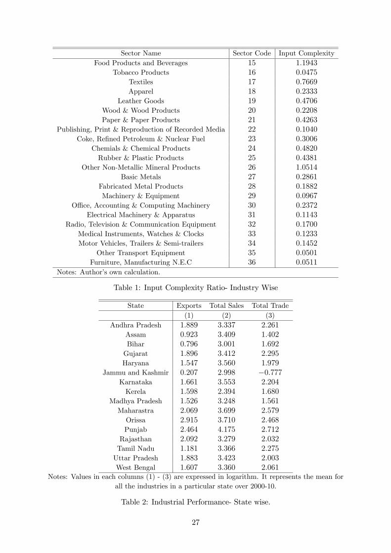
small percentage of firms are either government or foreign-owned. Table 1 calculates the“input-complexity”index at the two-digit level for each of the manufacturing sector using

‘power, fuel and electricity usage’of a firm as its intermediate input. Columns (1)—(3)

of Table 2 report the mean logarithm values of exports, total sales and total trade over

6

all the firms belonging to all manufacturing sectors for each of the major states of India

over 2000-10.

3.2 Data on Judicial Quality

I use judicial quality as the proxy for the institutional quality of a region or state. The

data on the variable indicating judicial quality is from the National Crime Records Bureau

(NCRB), which is an agency under Ministry of Home Affairs, Government of India,

responsible for collecting and analysing crime and judicial quality data as defined by the

Indian Penal Code (IPC). I use detail data from the NCRB’s Annual Crime in India

publication to construct my state-level judicial quality. This is the annual publication

of the Ministry of Home Affairs that gives the trends and patterns in judicial quality

throughout India. I choose one of the most important indicators which could bring

out a true and proper picture of the level of judicial effi ciency of a state —Number of

cases registered for trial under the Prevention of Corruption Act of a state. This annual

publication by the Ministry of Home Affairs reports information on the total number of

cases registered under the corruption act for trial at the courts for each state in any given

year. I assume that given the same level of judicial quality of all the states, the higher the

number of corruption cases, the lower is the judicial quality of a state. Therefore, focusing

on the cross state differences in judicial quality within a single country, I would be able

to thwart the common problems which arises with the cross-country studies. Columns

(1) and (2) of Table 3 report the mean values of judicial quality indicators across themajor states of India for 2000-10. I also use pendency ratio of all the cases (IPC plus

SLL2) at the lower courts for each of the different states in India as the alternate measure

of judicial quality. The results remain the same, however the magnitude of the effect

decreases.

Though the NCRB dataset comprises of all the states and union territories of India,

I choose to restrict our analysis for the 16 major states of India, primarily due to non-

availability of firm-level data for the small states and union territories for the entire period

of time. Nevertheless, these sixteen major states of India commands over 90 per cent of

the population and more than 85 per cent of the total industrial output produced in the

country.

4 Estimation strategy

My goal is to test whether judicial quality could serve as a source for comparative advan-

tage for firms’specializing in production of goods with higher proportion of intermediate2Special and Local Laws

7

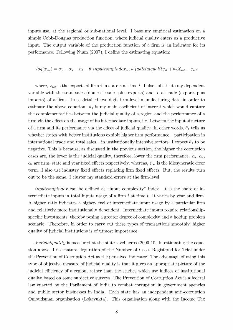
inputs use, at the regional or sub-national level. I base my empirical estimation on a

simple Cobb-Douglas production function, where judicial quality enters as a productive

input. The output variable of the production function of a firm is an indicator for its

performance. Following Nunn (2007), I define the estimating equation:

log(xist) = αi + αs + αt + θ1inputcompindexist ∗ judicialqualityst + θ2Xist + εist

where, xist is the exports of firm i in state s at time t. I also substitute my dependent

variable with the total sales (domestic sales plus exports) and total trade (exports plus

imports) of a firm. I use detailed two-digit firm-level manufacturing data in order to

estimate the above equation. θ1 is my main coeffi cient of interest which would capture

the complementarities between the judicial quality of a region and the performance of a

firm via the effect on the usage of its intermediate inputs, i.e. between the input structure

of a firm and its performance via the effect of judicial quality. In other words, θ1 tells us

whether states with better institutions exhibit higher firm performance —participation in

international trade and total sales —in institutionally intensive sectors. I expect θ1 to be

negative. This is because, as discussed in the previous section, the higher the corruption

cases are, the lower is the judicial quality, therefore, lower the firm performance. αi, αs,

αt are firm, state and year fixed effects respectively, whereas, εist is the idiosyncratic error

term. I also use industry fixed effects replacing firm fixed effects. But, the results turn

out to be the same. I cluster my standard errors at the firm-level.

inputcompindex can be defined as “input complexity” index. It is the share of in-

termediate inputs in total inputs usage of a firm i at time t. It varies by year and firm.

A higher ratio indicates a higher-level of intermediate input usage by a particular firm

and relatively more institutionally dependent. Intermediate inputs require relationship-

specific investments, thereby posing a greater degree of complexity and a holdup problem

scenario. Therefore, in order to carry out these types of transactions smoothly, higher

quality of judicial institutions is of utmost importance.

judicialquality is measured at the state-level across 2000-10. In estimating the equa-

tion above, I use natural logarithm of the Number of Cases Registered for Trial under

the Prevention of Corruption Act as the perceived indicator. The advantage of using this

type of objective measure of judicial quality is that it gives an appropriate picture of the

judicial effi ciency of a region, rather than the studies which use indices of institutional

quality based on some subjective surveys. The Prevention of Corruption Act is a federal

law enacted by the Parliament of India to combat corruption in government agencies

and public sector businesses in India. Each state has an independent anti-corruption

Ombudsman organisation (Lokayukta). This organisation along with the Income Tax

8

Department and the Anti-Corruption Bureau mainly helps to bring corruption amongst

the politicians and offi cers in the government service to public attention. The Act regis-

ters a case of corruption mainly when (a) a public servant taking gratification or valuable

things other than legal remuneration; (b) taking gratification in corrupt or illegal means

to influence a public servant; and (c) criminal misconduct by a public servant. Therefore,

the Act could be used as a powerful and important instrument determining the effi ciency

of the judicial institutions. Though, the number of cases does not really signify the exact

judicial quality in each state, nonetheless, it is one of the best indicators that can give an

idea about the governance situation of a state. Given the quality of the judicial system, I

assume that an act of corruption will certainly be detected by the judiciary of the state.

So, if the data suggests that the state X has higher number of cases on average registered

for trial than state Y, it would either mean that the governance quality is inferior in state

X or state X’s judiciary is ineffi cient. I interact my judicial quality variable with the

“input complexity” index to estimate whether states which have higher judicial quality

produces goods of higher institutional dependence.

Xist includes a rich set of control variables —judicial quality, intermediary share, var-

ious firm-level, industry-level and state-level characteristics, such as the skill and capital

intensity of a firm, age of a firm, age squared, ownership indicator, skill and capital en-

dowment of a state, income of a state, value-added by an industry and several others.

The inclusion of these various kinds of controls would help me to check whether my re-

sults still hold if I control for other measures of firm-level, industry-level and state-level

comparative advantage. However, one should still be careful in interpreting the basic

estimates as conclusive evidence about the effect of judicial quality on the dynamics of

firm performance because of the following two reasons: (a) reverse causality, and (b)

omitted variable bias. I explain the procedure of controlling these two problems in detail

as following.

4.1 Addressing Endogeneity of Judicial Quality

As mentioned before, two kinds of endogeneity problem may affect my results —reverse

causality and omitted variable bias. In order to control for the problem of reverse causality

in my estimations, I interact the judicial quality variable with the “input complexity”

index. To check for the robustness of results, I use one-period lagged values of judicial

quality. The results remain the same.

Another important concern with the estimation strategy is the omitted variable bias.

I address this issue by sequentially adding various state characteristics and its interac-

tion with “input complexity”index to my baseline specification. In other words, it can

be argued that the differential effect of “input complexity” index on firms in different

9

states may be due to other state factors that are unrelated to judicial quality. There-

fore, by adding proxies of alternate state characteristics and its interaction with “input

complexity” index, I am able to test whether the performance premium due to more

effi cient judiciary is robust to controlling for these additional channels. In addition to

these control variables, the inclusion of state fixed effects in the baseline specification will

also control for time-invariant state characteristics but not for time-varying unobservable

characteristics. For example, it may be the case that a firm’s exports or total sales and a

state’s judicial quality are correlated with the economic and political condition. I also add

state—year interaction fixed effects to my baseline specification to examine whether the

main results are robust to controlling for time-varying, unobservable state characteristics.

A related and crucial issue is the self-selection problem of firms. The firms may

self-select themselves in states which have effi cient judiciaries, i.e. if a bigger exporter is

located in a state with more effi cient judiciary and use a higher proportion of intermediate

inputs, then the results of this paper will reflect nothing, but a simple spurious correlation.

This could potentially bias my results. Following Ahsan (2012), I compare the exports of

firms in high judicial quality states (judicial quality above the sample median) with the

exports of firms in low judicial quality states (judicial quality below the sample median).

I find no evidence to suggest that high performance firms locate in high judicial quality

states.3 I also do not observe any evidence of systematic agglomeration in the data,

which could also raise some serious concerns about the identification strategy used in this

paper. The industries included in the sample are fairly well spread across the various

states. Thus, the potential selection of high performing firms in high judicial quality

states that also experience higher intermediate input usage, as a likely explanation for

the results documented in this paper is bleak.

Nonetheless, in order to be profoundly convinced that self-selection of firms does not

play any role in the results of this paper; I carry out the following exercise: I estimate the

effect of judicial quality on the firm performance using a pseudo-2SLS4 type of method,

utilizing the matching estimator technique. In order to do this, I use the propensity

score matching (Rosenbaum and Rubin, 1983) method to generate propensity scores in

the first stage and then estimate the average treatment effect of the judicial quality —

by weighing with the inverse of a nonparametric estimate of the propensity score rather

than the true propensity score —on the performance indicator of a firm. This leads to

an effi cient estimate of the average treatment effect (Hirano et al., 2003). To generate

propensity scores, I do the following: I construct a control group of firms in states with

low judicial quality that has observable firm characteristics5 similar to that of firms in3I do not also find any such evidence for total sales and total trade as well.4Two Stage Least Squares5By observable firm characteristics, I mean age, age-squared, ownership and assets (big or a small

firm) of a firm.

10

states with high judicial quality. By matching firms in this manner I reduce any bias

that may arise due to systematic observable differences between firms in states with high

judicial quality and firms in states with low judicial quality. I then match firms in high

and low judicial quality states using this propensity score matching. To implement this,

I first calculate the sample median for the corruption cases registered for trial for all the

states for each of the year. I then use each state’s average value of the corruption cases

registered for trial in a year (averaged over 2000—10) to classify it as having high or low

judicial quality. In particular, if a state’s average number of corruption cases is equal

to or greater than the sample median in the base year of the analysis, it is classified as

having low judicial quality. I take the median value of the states in 2000 in order to

control for further endogeneity, since states may change its position in terms of judicial

quality over the period of analysis. If a state’s average number of corruption cases is

below the sample median it is classified as having high judicial quality. Next, using this

information I construct an indicator variable judquai that is one if firm i is in a state at

or below the sample median judicial quality and zero otherwise. This indicator variable

is then used to construct propensity scores by estimating the following probit model:

Pi = Pr{judquai = 1 | Yit, perindicit} = Φ{γ1Yit + γ2perindicit}

whereΦ{∗} is the normal cumulative distribution function, Yit are the control variablesincluding the natural logarithm of age, age squared, government or foreign ownership and

size indicator. perindicit is the performance indicator of a firm —exports, total trade and

total sales. Thus, firms are matched based on their characteristics including exports,

total sales and total trade. The propensity scores, Pi, thus generated is the conditional

probability of receiving a treatment by a firm given pre-treatment characteristics, Yit.

These estimated propensity scores can be used to estimate the average treatment effects

in different ways —nearest matching method, radius matching, kernel matching method

and stratification method. I choose to use the nearest matching method for my purpose.

Let T be the set of treated (high judicial quality) units and C the set of control (low

judicial quality) units, and ZTi and Z

Cj be the observed outcomes of the treated and control

units, respectively. I denote C(i) as the set of control units matched to the treated unit

i with an estimated propensity score of P̂i. I now use the estimated propensity scores,

P̂i, to match each firm in a state with high judicial quality (treatment) with its nearest

neighbour among firms in states with low judicial quality (control). In other words, for

each pair I minimize

C(i) = min || P̂i,T − P̂i,C ||

11

where P̂i,T and P̂i,C are the estimated propensity scores of a firm in a state with high

judicial quality and its nearest neighbour in a state with low judicial quality, respectively.

This balancing exercise produces a sample of firms that are similar based on a set of

observable controls. This difference above is a singleton set unless there are multiple

nearest neighbours. In practice, the case of multiple nearest neighbours should be very

rare, in particular if the set of characteristics Yit contains numerous continuous variables;

the likelihood of multiple nearest neighbours is further reduced if the propensity score

is estimated and saved in double precision. I use this matched sample weighing by the

inverse of the non-parametric estimate of the propensity score to estimate the average

treatment effect in the following way. Using the nearest matching method, I denote the

number of controls matched with observation i ε T (treated units) by NCi and define the

weights ωij = 1NCiif j ε C(i) and ωij = 0 otherwise. I estimate the following equation

with the inverse of the estimated propensity score to examine the average gains of the

treated units accrued from the treatment:

τM = 1NT

∑iεT

Y Ti − 1

NT

∑ωj

jεC

Y Cj

where, τM is the gain from the average treatment effect due to the nearest neigh-

bour matching method and ωj =∑i

ωij. I report bootstrapped standard errors (100

repetitions) for the estimates from the average treatment effect.

5 Results

5.1 Basic Results

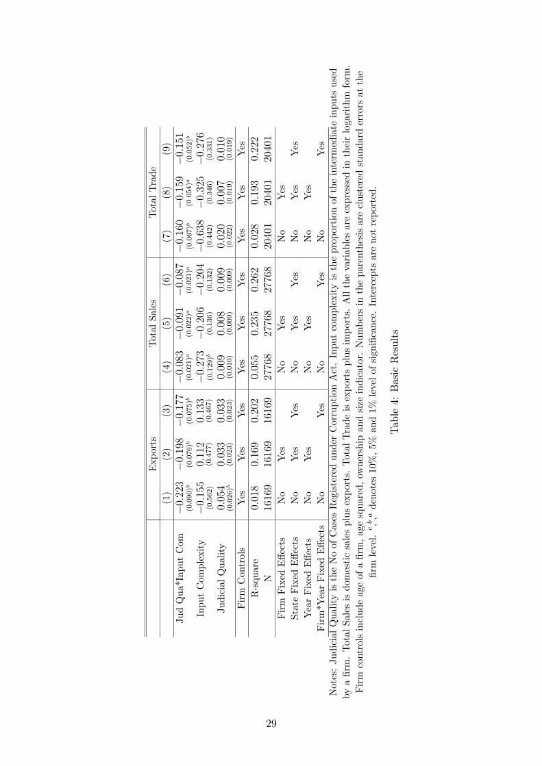
Table 4 examines the overall relationship between judicial quality and firm performance.I use three different indicators for firm performance —exports, total total trade (exports +

imports) and total sales (exports + domestic sales), with main focus being on exports. My

ordinary least squares (OLS) estimates produces negative coeffi cient for all the cases. This

indicates that higher judicial quality leads to higher firm performance through specializing

inputs, which require relation-specific investments. Column (1) regress judicial quality

on the natural logarithm of total exports of a firm not controlling for any other effects —

be it observable or unobservable firm, state and year characteristics. The point estimates

suggest that higher judicial quality is significantly associated with higher total exports of

a firm at 5 per cent level of significance. The results suggest that a firm located in a high

judicial quality region export goods which relies more on institutional dependent inputs.

In other words, better quality of governance help the firms to invest in intermediate goods

12

through reducing the idiosyncratic risk involved. Therefore, it can be conjectured that

the judicial quality benefits a firm in overcoming the hold-up problem and produce higher

level of output and engage in higher level of international trade. In column (2), I add

firm, state and year fixed effects, the results remain the same. However, the value of the

coeffi cient decreases slightly. In column (3), I check the robustness of the results by adding

state fixed effects and interaction of firm and year fixed effects to my baseline specification.

These interaction effects control for unobservable, time-varying firm characteristics that

are potentially correlated with "input complexity" index and firm sales. As the results

demonstrate, the inclusion of these interaction effects also does not significantly alter the

baseline specification. One standard deviation change in judicial quality would increase

the exports of firm by 0.25-0.31 standard deviation based on the specification used. My

results are in complete conformity with the standard cross-country results of estimating

the impact of a country’s institutions on economic performance (Knack and Keefer, 1995,

1997; Hall and Jones, 1999; Levchenko, 2007; Nunn, 2007). My estimates are also very

close to what Laeven and Woodruff (2007) find using firm-level data on Mexico about

the effect of quality of legal system on firm size.

In columns (4)—(6), I use natural logarithm of total sales of a firm as an indicator

for firm performance. The total sales of a firm have been defined as the summation of

exports and domestic sales. The sign and significance level of the coeffi cients remain

the same, but the value of point estimates decrease by around half of that of exports. I

continue to check my results by adding different sets of fixed effects. Likewise the results

on exports, the estimates on total sales also do not change. In this case, one standard

deviation change in judicial quality increases total sales of a firm by 0.12-0.13 standard

deviation.

In columns (7)—(9), I add total imports of a firm with total exports, thereby having

total trade of a firm as the performance indicator. I use natural logarithm of total trade

as the dependent variable. I find significant effect of judicial quality on the total trade of

a firm. The effect remains the same, irrespective of the specification I use. The results

suggest that the total trade of a firm increases by 0.21-0.22 standard deviations with one

standard deviation change in the judicial quality, depending on the specification. Though

there is some amount of literature focusing on the effect of judicial quality on exports at

the firm-level, however there is a dearth of studies which focuses on the total trade or

imports. However, research at the macro level shows that judicial quality has a positive

effect on the total trade of the countries’.

In Table 5, I test the robustness of the above result by including other firm and

industry characteristics and allowing the effect of judicial quality to vary along some ad-

ditional dimensions. The inclusion of these additional variables address the fact that the

13

performance of Indian firms may be correlated with factors that drive India’s patterns

of comparative advantage. In columns (1)—(3), I test the effect for exports, in (4)—(6),

for total sales of a firm and finally columns (7)– (9) use total trade as the performance

indicator. Column (1) adds each firm’s capital intensity and its interaction with judicial

quality. Capital intensity is defined as the amount of capital used by each firm. I use

natural logarithm of the capital used by a firm for the estimation. As the results demon-

strate, the inclusion of this additional control does not alter the coeffi cient of interest.

It continues to be significant at 5 per cent level. In column (2), I add each firm’s skill

intensity interacted with judicial quality. Skill intensity of a firm is defined as the natural

logarithm of total salaries and wages paid by each firm towards the total compensation

for their employees. Once again, the primary coeffi cient of interest remains robust. Next,

in column (3), I add each industry’s concentration ratio and its interaction with judicial

quality. Concentration ratio is defined as the logarithm of output of an industry. I match

state-wise Annual Survey of Industries (ASI) data (described in detail in Section 6) at

the two-digit level with the firm-level data in order to use the concentration ratio as one

of the explanatory variables. The inclusion of this additional control also has minimal

effects on the primary coeffi cient of interest.

Columns (4)—(6) do the same estimations using total sales of a firm as the output

variables. The value of the coeffi cients decrease, but the effect remains robust. However,

I find some two additional result —(i) capital intensity of a firm being significantly and

positively affecting the performance of a firm. However, the effect is very small; and

(ii) firms’experience a higher value of total sales, which belong to industries of higher

value of output. Columns (7)—(9) use total trade as the left-hand side variable. My

primary coeffi cient of interest remains the same. I continue to find positive effect of

capital intensity of a firm.

5.2 Industry and State Characteristics

If the differences in judicial quality are really driven by other characteristics of the states,

my results would be biased, if I do not control for them. Table 6 presents a separateset of results controlling for all possible state characteristics and its interaction with

firm choice variables. Column (1) introduce both skill and capital endowment of a state

and its interaction with the skill and capital intensity of firm, respectively to control

for the factor endowments of a state. Skill endowment of a state is measured by the

literacy rate of a state, whereas capital endowment is sum of fixed, invested and working

capital of the entire manufacturing sector of a state. The primary result of judicial

quality being positively affecting the firm exports continue to hold at 5 per cent level of

significance. However, the estimates from column (1) also suggest an important result

14

from the perspective of H-O model of trade, where factor endowments play a very crucial

role in determining the pattern of trade. In this case, judicial quality turns out to be the

most significant factor. My findings are in complete allegiance with the recent theory of

comparative advantage, where institution is cited as one of the major determining factors

of the production pattern of a region (Levchenko, 2007; Nunn, 2007).

Next, I control for another important characteristic of a state which might affect

the overall firm performance. This, if omitted, may bias my estimated importance of

judicial quality as a factor of comparative advantage for the production of institutionally-

dependent manufacturing goods. I interact the gross value-added of an industry with the

income per capita for a given Indian state in column (2) to control for the possibility

that the high income regions might specialize in high value-added industries. Gross

value-added is defined as total value of output minus the raw material costs. I use gross

value-added data from the ASI database at the two-digit level upon matching with the

firm-level data. The results do not produce any evidence of significant impact of high

income regions to be a key factor for a firm engaging in international trade. I substitute

exports with total sales of a firm in columns (3) and (4), the results remain the same.

Judicial quality continues to the most important factor affecting the total sales of a firm

at 1 per cent level of significance. I also use total trade as a performance indicator

in columns (5) and (6) controlling for important firm, state and year characteristics. I

continue to find significant evidence in support of the fact that judicial quality affects the

total trade of a firm. Column (5) also confirms the importance of capital endowment of

a region in influencing the total amount of international trade of a firm.

To test the robustness of my results, I extend my analysis to control for several other

alternate state characteristics in Table 7. Column (1) includes total factor productivity(TFP) growth of the industry as one of the key determinants of comparative advantage

of the firm performance. The TFP is calculated using the Levinshon and Petrin (2003)

methodology6 from the ASI database. The judicial quality continues to significantly and

positively affecting a firm’s international trade activity at 10 per cent level. I do not seem

to find any effect of the productivity growth of an industry on a firm’s performance. Fol-

lowing Nunn (2007), I include another important characteristic, the interaction between

per-capita income of a state and input variety in column (2) in order to estimate if highly

developed regions use different types of inputs. I calculate input variety as one minus

the Herfindahl index of input concentration for each industry. This measure increases

in the variety of inputs used in production. It is also generally used to measure the

‘self-containment’of an industry. The backward regions, which have poorly developed

infrastructure, tend to specialize in industries that are “self-contained”. It is opposite of

6For details, please see Levinshon and Petrin (2003).

15

the measure “input complexity”. In other words, regions with high quality of judicial in-

stitutions would specialize in complex goods, which will rely heavily on institutions than

simple goods. My results confirm that a state with high-quality institutions significantly

specializes more in complex goods.

In columns (3) and (4), I interact the factor endowment variables with the “input-

complexity” index in order to control for situations, where higher skill endowment or

capital endowment regions might manifest in industries which have a higher dependency

on intermediate inputs. I find none of them to be significantly determining a firm’s export

behaviour. To control for financially developed states, I use a binary measure of financial

development following Khandelwal and Topalova (2011) in column (5). The states whose

average per capita credit is above the median per capita credit of India are classified

as the financially developed states, and otherwise. It could be possible that financially

developed regions might specialize in goods with a complex input structure. I fail to

find any such evidence. Columns (6)—(10) repeat the estimations from columns (1)—(5)

by using total sales of a firm as the performance indicator. In column (6), I find that

firms’belonging to industries of higher productivity growth do have higher total sales.

Column (7) confirms that states with high judicial quality significantly specializes more

in complex goods. Column (10) finds that financially developed states register a higher

volume of total firm sales, with the primary result being the same. I also do the same

exercises for the total trade of a firm (results not reported). The primary result of interest

continues to hold even when I control for different industry and state channels in case of

total trade of a firm.

5.3 Other Industry Characteristics

If differences in the judicial quality are really driving the results we observe so far, I

should not find any such effect for non-contractive industries. Next, I divide the industries

into —contractive and non-contractive. In particular, if certain industries need a higher

proportion of intermediate inputs usage, then firms in those industries are more likely

to be dependent on quality of judiciary. In Table 8, I distinguish between contract-intensive and non-contract intensive industries. Contract intensive industries are defined

as those which have greater than median “input-complexity”index of the sample, while

the remaining as non-contract intensive industries. The results strongly suggest that the

complementarities between “input-complexity”index and judicial quality accrue only in

contract-intensive industries. Even when I control for several state-level channels, the

results hold. The results indicate that the complementarities between judicial quality

and gains from either firm exports or sales are strongest for firms in contract intensive

industries, i.e., the firms which have a higher usage of intermediate inputs.

16

5.4 Alternate Judicial Quality Indicator

In this section, I use a different indicator of judicial quality to see if the results demon-

strated above behave in the same pattern irrespective of the indicator, i.e., if my results

are robust to any alternate type of judicial indicator I use. Table 9 presents the requiredresult. I use the pendency ratio of all the cases (IPC plus SLL) for the lower courts of

the Indian states. The ratio is defined as the number of cases pending at the end of the

year divided by the total number of cases of that year. I include the SLL cases, because

it comprises the lion’s share of all the cases, so focusing only on IPC cases would entail

a significant bias on the effectiveness of the judicial quality indicator. The number of

pending cases in the lower courts of a state is primarily a function of the ability of the

judges appointed by the respective state governments. While the state High Court ap-

pointments are made at the federal level, state governments control the administration of

the state legal system, i.e., of the local courts, with limited supervision from the Supreme

Court of India. This may result in significant amount of heterogeneity across different

states with regard to the speed and effi ciency with which the cases are persuaded. The

rules and regulations at all the levels of the legal system are outlined by the Code of Civil

Procedure, which is uniform across all states. But, significant differences could appear

over time regarding the manner in which the rules and procedures are implemented in

each state (Kohling, 2000). The main difference is due to the common law system that is

used in India, which provides the High Court judges with a greater degree of flexibility in

interpreting certain rules and procedures. As a result, differences in High Court interpre-

tations can lead to significant variation in the interpretation of rules and procedures over

time. Thus, the state courts in India could vary along the differences in the implemen-

tation of rules and procedures which in turn could effect the state-run administration.

I also use a different indicator for the labour endowment of a state in order to see how

sensitive the results are also to the use of different indicators for different arguments of

the production function. I use the stock of the production workers of a state. All the

other variables remain the same.

Column (1) regress total exports of a firm on the judicial quality and its interaction

with the proportion of intermediate input usage. The results show that judicial quality

continues to have positive and significant effect on a firm’s international trade activity.

The reason is may be due to the importance of a court’s activity to the intermediate input

supplies. A good legal system provides confidence to firms by acting as a facilitator, in

the sense that firms know that if the negotiations break down, they could always pursue

their dispute through the courts. Therefore, faster disposition of the cases by courts give

assurance to the firms that they have a back-up option if other methods fail. Thus, courts

can have direct and indirect effects on dispute settlement. The results also show that

the firms located in high income regions experience higher earnings from trade. Columns

17

(3) and (4) introduce skill endowment and capital endowment and its interaction with

input complexity, respectively. My primary result continues to hold at 1 per cent level

of significance. Substituting the dependent variable exports with total sales of a firm in

columns (4)—(8) do not alter the demonstrated results.

5.5 Addressing Endogeneity of the Judicial Quality Indicator

Next, I address the concern for the self-selection effect of the firms. That is, the results

demonstrated so far in this paper can be biased by the self-selection of the firms in states

with higher judicial quality. The issue is discussed in greater detail in section 4.1. In

particular I use a matching estimator to match firms based on similar characteristics. I

generate a control group of firms in states with low judicial quality that has characteristics

similar to firms in states with high judicial quality. I regress the judicial quality indicator

(which takes a value 1 for states with high judicial quality, i.e., for states with less cases of

corruption than the median) on the various state characteristics and generate propensity

scores. I use the inverse of those propensity scores to estimate the average treatment

effect of the firms from the treated (high judicial quality) zone on the exports and total

sales7. The results using matched sample are listed in columns (1)—(4) of Table 10. Imatch the firms based on several firm characteristics like the age, age squared, ownership

and size indicator. The coeffi cients from column (1) suggest that higher judicial quality

significantly propels higher exports for firms in states with high judicial quality when

compared to firms in states with low judicial quality. The value of the estimated coeffi cient

at the second stage increases. This suggests that not controlling for self-section effect may

have a downward bias on the estimated effect of judicial quality on trade flows.

Next, I examine whether this result is biased by time-varying, unobservable firm

characteristics that are potentially correlated with the firm exports and the usage of

intermediate inputs. I add firm-year interacted fixed effects to the baseline specification

in column (1). The coeffi cient of interest is negative and significant. However, the point

estimates decreases by some magnitude. This demonstrates that not controlling for time-

varying firm unobservable characteristics may somewhat overestimate the effect. I do

not need to separately control for time-varying unobservable state characteristics as the

average treatment effect method takes care of it automatically. However, I do control

for factor endowment variables and the development indicator of a state in a separate

estimation, but the results do not change (not reported). These results also confirm that

even when controlling for these differences, judicial quality continues to be an important

determinant of comparative advantage.

7I also run the same exercise for total trade. The results are the same (not reported).

18

I do the same for the total sales of a firm in columns (3)—(4) to test if the effect is robust

to a different performance indicator of a firm. Once again, the effect remains negative

and significant at 1 per cent level. In this case as well, the point estimate decreases when

I control for time-varying unobservable firm characteristics. Judicial quality continues

to be the most effective for exports, least for total sales with total trade in between.

The results in columns (1)—(4) of Table 10 are based on a restricted sample of firms instates with high judicial quality and their nearest neighbours with low judicial quality.

This matching process creates a sample of firms, which are similar based on observable

characteristics. While the firms across the treatment and the control groups may differ

based on unobservable characteristics, the use of a matched sample is likely to reduce

the bias arising due to the self-selection process of the firms into those particular states

(Ahsan, 2012).

Next, I use a different method to further control for the endogeneity (in particular

reverse causality problem) of the judicial quality. I use one year lag value of the judi-

cial quality to attenuate the bias that may arise because of the reverse causality effect.

Though, I already control for the problems of reverse causality by using an interaction

effect of the variable of interest, but, I additionally do this in order to be more convinced

and further check the robustness of my results. Columns (5)—(9) use one-period lag value

of judicial quality as an instrument for the current period. The results are in complete

sync with the earlier results. Judicial quality continues to significantly and positively

affect the exports of firms in goods which are institutionally dependent. However, in this

case, I find some evidence of the fact that high income regions and firms’having higher

skill intensity experience higher export earnings, but the effect is not robust. I continue

to find capital intensity to be a significant factor affecting the exports of a firm.

6 Robustness Checks

In Table 11, I check the robustness of my earlier results by using alternative methods,sample and dataset. In column (1), I use Average Treatment Effect (ATE) method. The

ATE measures the difference in mean (average) outcomes between the units assigned to

the treatment and control group, respectively. Since, ATE averages across gains from

units, I use average treatment effect on the treated (ATT), which is the average gain

from treatment for those who actually are treated. I utilize the previous classification of

firms into high judicial quality states and low judicial quality states as the treatment and

the control group, respectively. I estimate the following equation to calculate the gain

from ‘treatment’:

τATT = E[Y (1)− Y (0) | W = 1]

19

where, τATT denotes the gain received by the firms which belong to the state of higher

judicial quality. The expected gain is assumed to be in response to the randomly selected

unit (firms) from the population. This is called the average treatment effect of the treated.

Y (1) is the outcome with the treatment and Y (0) is without the treatment. The binary

“treatment”indicator is W , where W = 1 denotes “treatment”. I use natural logarithm

of exports of a firm as the response variable of a result of the treatment . As previously, I

expect the coeffi cient on trade performance to be negative, which indicates positive gain

for firms in states with higher degree of judicial quality. Everything else being equal,

the firms in the high judicial quality regions are supposed to have earnings from exports

which are higher than firms of regions of lower degree of judicial quality. That is, relative

to the states which are of low judicial quality, high judicial quality states are expected

to trade or produce relatively more in institutional-dependent industries. I estimate the

above equation by considering a sample of all possible sample pairs. I cluster the stan-

dard errors at the firm-level. I estimate by matching high judicial quality and low judicial

quality states based on skill intensity, capital intensity, value added by an industry, skill

endowment, capital endowment and income of a state. The reason I do this is that —

the high and low judicial quality states could be different in ways other than the judicial

quality classification, and these differences may be important for comparative advantage,

which could bias my estimates. By restricting my sample to matched state pairs, I poten-

tially remove bias that could exist in my estimates if the state characteristics are ignored.

Column (1) reports the estimates of the average treatment effect of the treated, when

state pairs are matched by skill and capital intensity, skill and capital endowment. The

estimates confirm that the higher earnings from engagement to international trade accrue

to firms of high judicial quality regions significantly. Column (2) additionally controls

for the value added by an industry and income of a state. The effect remains the same,

however, the coeffi cients increase. This suggests income to be a significant contributing

factor for the gains of a firm, and therefore, not controlling for it will underestimate

my coeffi cients. The results prove that judicial quality continues to a significant factor

of comparative advantage for firms’production of goods using institutionally dependent

inputs, even when controlling for all the other major differences between regions. The

average treatment effect results provide further evidence that judicial quality and insti-

tutionally dependent inputs are important and complementary determinants of higher

industrial output.

In column (3), I examine whether my results are robust to dropping various states

from the sample. In particular, I drop firms located in Maharashtra, a state which

includes around 34 per cent of the firms in the sample primarily due to its size and the

fact that it is the state where Mumbai Stock Exchange is located. The results are robust

to the exclusion of that particular state. Column (4) test if the results are robust to

20

the exclusion of the outliers. Outliers are defined as observations for which the absolute

values of studentized residuals are above two. The results indicate that even after outliers

have been dropped the interaction between “input-complexity”index and judicial quality

remains negative and significant. In columns (5) and (6), I drop states which are at the

top and bottom 15 per cent of the judicial quality distribution, respectively. In both the

cases, the coeffi cient remains negative and significant.

In columns (7)—(9), I use a different dataset for a different period of time to check,

whether my results demonstrated above are robust irrespective of the dataset and the

period of analysis. And also, if the results do hold for the firm-level dataset, it should

also hold for the industrial level dataset as well. For columns (7)—(9), I use two-digit level

manufacturing data from the Annual Survey of Industries (ASI) for the major states for

the period 1981-1998. The data set is compiled by the Central Statistical Organisation,

(CSO), Ministry of Statistics and Program Implementation, Government of India. It is

a very comprehensive annual survey of Indian manufacturing plants. The ASI reports

data for the organised segments of registered manufacturing under Sections 2m (i) or

2m (ii) of the 1948 Factories Act. The ASI sampling population covers factories using

power employing 10 or more (permanent and production) workers, and factories without

power employing 20 or more workers. It records detail industrial level data at two-digit

level. The data reports almost all the principal characteristics8 at the two-digit industry

level for all the manufacturing industries. But, it does not report an industry’s activity

towards international trade, i.e., either exports or imports. Therefore, I choose to use

the total output of an industry as the left-hand side variable or the performance indica-

tor. I continue to use the expenditure incurred by an industry towards fuels, lubricants,

electricity and water consumed as the intermediate inputs.

For this case, I construct a judicial quality index by putting together Number of cases

registered under the Corruption Act and Pendency ratio of the lower courts of a state

using Principal Component Analysis (PCA) technique. The different judicial quality

indicators are measured in different magnitude. While, the pendency ratio of courts is

a unit free ratio, the number of corruption cases registered for trial is a count variable.

Therefore, in order to build a unified index, first, I normalize them. This is done to have a

common unit and to get the relative position of each state with respect to judicial quality.

The normalized values lie between 0 and 1. Once the normalized values are obtained, I

compute the factor loading and weights of these indicators. I derive the composite index8Number of Factories, Fixed Capital, Working Capital, Physical Working Capital, Productive Capi-

tal, Invested Capital, Outstanding Loans, Number of Workers, Mandays-Workers, Number of Employees,Mandays-Employees, Total Persons Engaged, Wages to Workers, PF and Other Benefits, Total Emol-uments, Fuels Consumed, Materials Consumed, Total Inputs, Rent Paid, Interest Paid, Depreciation,Value of Products and By-Products, Value of Gross Output, Net Income, Profits, Net Value Added,Gross Value Added, Net Fixed Capital Formation, Gross Fixed Capital Formation, Additions to Stock,Gross Capital Formation

21

by multiplying the weights with the normalized values of each of the judicial quality

measure. Since, the principal component index is built on the basis of factor loadings,

the higher the numbers of different components are, the higher would be value of the

index. And, since higher values for both the indicators indicate a low judicial quality,

therefore, the higher value of the index of a state indicates low judicial quality of that

state. Likewise our previous results, I also expect a negative coeffi cient of the effect of

judicial quality on industrial performance.

Column (7) regress the natural logarithm of industrial output on the interaction be-

tween the constructed judicial quality index and intermediate input usage, controlling

for state, industry and year unobservable characteristics. The estimate turns out to be

negative and significant, indicating that the judicial quality continues to be positively

affecting the industrial performance of a state. Column (8) introduces skill and capital

endowment and income of a state in addition to state industry and year fixed effects.

The results do not change. Finally, in column (9), I control for further for industry and

state characteristics by interacting input-complexity index with skill endowment, capital

endowment and financial development of a state. The financial development indicator

has been taken from Khandelwal and Topalova (2011). However, my primary result does

not change. It produces two additional results as well —skill endowment and financial

development of a state are also significant determinants of comparative advantage for the

industrial output.

7 Conclusion

This paper complements a gap in the literature by addressing the complementarities be-

tween judicial quality and the usage of intermediate inputs on firm performance, especially

exporting behaviour. It uses a firm-level panel data from India for the period 2000-10

along with objective measures of judicial quality at the state level. Since, India offers suf-

ficient amount of heterogeneity involved among different regions within a single country

framework, therefore, it provides an ideal setting to examine the hypothesis posed in the

paper. I find judicial quality to be a significant factor for firm performance, especially

exports and total trade flows. The results also suggest that the effect is strongest for

firms which belong to industries, which are more contract-intensive, i.e., the ones which

require more institutionally dependent inputs. I also find capital endowment to be an

important factor for firm earnings from international trade. High income states register

higher total sales by the firms. The results are robust to using a matching estimator tech-

nique to address the self-selection problem of firms into states with high judicial quality

and using lagged values of the judicial quality. In addition, the results are also robust

to the inclusion of various time-varying state, firm level observables and unobservable

22

characteristics (i.e., state-year and firm-year fixed effects). The results are also robust

irrespective of different samples, different dataset or the period of analysis. Thus, the

results confirm that judicial quality is necessary for firms to invest in intermediate inputs

in order to maximize benefits from its participation in international trade.

23

References

[1] Acemoglu, D., S. Johnson, J. Robinson, (2001), “The Colonial Origins of Com-

parative Development: An Empirical Investigation”, American Economic Review, 91 (5),

pp. 1369-1401

[2] – ., (2002), “Reversal of Fortune: Geography and Institutions in the Making of

the Modern World Income Distribution”, Quarterly Journal of Economics, 117 (4), pp.

1231-94

[3] Ahsan, R. N., (2012), “Input Tariffs, Speed of Contract Enforcement, and the Pro-

ductivity of Firms in India”,Mimoegraph, University of Melbourne, Melbourne, Australia

[4] Antras, P., (2003), “Firms, Contracts and Trade Structure”, Quarterly Journal of

Economics, 118 (4), pp. 1375-1418

[5] – ., (2005), “Incomplete Contracts and the Product Cycle”, American Economic

Review, 95 (4), pp. 1054-73

[6] Costinot, A., (2009), “On the Origins of Comparative Advantage”, Journal of

International Economics, 77 (2), pp. 255-64

[7] Cowen, K., A. Neut, (2007), “Intermediate Goods, Institutions and Output Per

Worker”, Central Bank of Chile Working Paper No 420, Central Bank of Chile, Santiago

[8] Do, Quy-Toan., A. Levchenko, (2006), “Trade, Inequality, and the Political Econ-

omy of Institutions”, Journal of Economic Theory, 144 (4), pp. 1489-1520

[9] Felipe, J., U. Kumar, (2010), “Technical Change in India’s Organized Manufactur-

ing Sector”, Levy Economics Institute Working Paper No. 626, Levy Economics Institute,

New York, USA

[10] Goldberg, P., A. Khandelwal, N. Pavcnik, P. Topalova, (2010), “Imported Inter-

mediate Inputs and Domestic Product Growth: Evidence from India”, Quarterly Journal

of Economics, 125 (4), pp. 1727-67

[11] Grossman, S. J., O. D. Hart, (1986), “The Costs and Benefits of Ownership: A

Theory of Vertical and Lateral Integration”, Journal of Political Economy, 94 (4), pp.

691-719

[12] Hall, R. E., C. Jones, (1999), “Why do some countries produce so much more

Output per worker than Others?”, Quarterly Journal of Economics, 114 (1), pp. 83-116

[13] Halpern, L., M. Koren, A. Szeidl, (2009), “Imported Inputs and Productivity”

CEPR Discussion Paper 5139, CEPR, London, UK

[14] Hart, O. E., J. Moore, (1990), “Property Rights and the Nature of the Firm”,

Journal of Political Economy, 98 (6), pp. 1119-58

[15] Hirano, K., G. W. Imbens, G. Ridder, (2003), “Effi cient Estimation of Average

Treatment Effects Using the Estimated Propensity Score”, Econometrica, 71 (4), pp.

1161-89

[16] Kasahara, H., J. Rodrigue, (2008), “Does the use of imported intermediates

24

increase productivity? Plant-level evidence”, Journal of Development Economics, 87 (1),

pp. 106-18

[17] Keefer, P., S. Knack, (1995), “Institutions and Economic Performance: Cross

Country Tests using Alternative Institutional Measures”, Economics and Politics, 7 (3),

pp. 207-27

[18] – , (1997), “Why Don’t Poor Countries Catch Up? A Cross-National Test of

Institutional Explanation”, Economic Inquiry, 35 (3), pp. 590-602

[19] Khandelwal, A., P. Topalova, (2011), “Trade Liberalization and Firm Productiv-

ity: The Case of India”, The Review of Economics and Statistics, 93 (3), pp. 995-1009

[20] Kohling, W., (2000), “The Economic Consequences Of A Weak Judiciary: In-

sights From India”, Law and Economics 0212001, Economics Working Paper Archive at

WUSTL, Washington University in St. Louis, USA

[21] La Porta, R., F. Lopez-de-Silanes, A. Shleifer, R. Vishny, (1997), “Legal Deter-

minants of External Finance”, Journal of Finance, 52 (3), pp. 1131-50

[22] – , (1998), “Law and Finance”, Journal of Political Economy, 106 (6), pp. 1113-

55

[23] Laeven, L., C. Woodruff, (2007), “The Quality of the Legal System, Firm Own-

ership, and Firm Size”, The Review of Economics and Statistics, 89 (4), pp. 601-14

[24] Levchenko, A., (2007), “Institutional Quality and International Trade”, Review

of Economic Studies, 74 (3), pp. 791-819

[25] Levinsohn, J., A. Petrin, (2003), “Estimating Production Functions Using Inputs

to Control for Unobservables”, Review of Economic Studies, 70 (2), pp. 317-42

[26] Mundle, S., P. Chakraborty, S. Chowdhury, S. Sikdar, (2012), “The Quality of

Governance: How Indian States Performed?”, Economic & Political Weekly, 47 (49), pp.

41-52

[27] North, D., R. Thomas, (1973), The Rise of the Western World: A New Economic

History, Cambridge University Press, Cambridge, UK

[28] North, D., (1981), Structure and Change in Economic History, W. W. Norton &

Company, New York

[29] North, D., (1994), “Economic Performance Through Time”, American Economic

Review, 84 (3), pp. 359-68

[30] Nunn, N., (2007), “Relationship-Specificity, Incomplete Contracts and the Pattern

of Trade”, Quarterly Journal of Economics, 122 (2), pp. 569-600

[31] – ., (2009), “The Importance of History for Economic Development”, Annual

Review of Economics, 1 (1), pp. 65-92

[32] Rosenbaum, P. R., D. B. Rubin, (1983), “The central role of the propensity score

in observational studies for casual effects”, Biometrika, 70, pp. 41-55

[33] Segura-Cayuela, R., (2006), “Ineffi cient Policies, Ineffi cient Institutions and Trade”,

Banco de Espana Research Paper WP-0633, Bank of Spain, Madrid, December 2006

25

26

Sector Name Sector Code Input ComplexityFood Products and Beverages 15 1.1943

Tobacco Products 16 0.0475Textiles 17 0.7669Apparel 18 0.2333

Leather Goods 19 0.4706Wood & Wood Products 20 0.2208Paper & Paper Products 21 0.4263

Publishing, Print & Reproduction of Recorded Media 22 0.1040Coke, Refined Petroleum & Nuclear Fuel 23 0.3006

Chemials & Chemical Products 24 0.4820Rubber & Plastic Products 25 0.4381

Other Non-Metallic Mineral Products 26 1.0514Basic Metals 27 0.2861

Fabricated Metal Products 28 0.1882Machinery & Equipment 29 0.0967

Offi ce, Accounting & Computing Machinery 30 0.2372Electrical Machinery & Apparatus 31 0.1143

Radio, Television & Communication Equipment 32 0.1700Medical Instruments, Watches & Clocks 33 0.1233Motor Vehicles, Trailers & Semi-trailers 34 0.1452

Other Transport Equipment 35 0.0501Furniture, Manufacturing N.E.C 36 0.0511

Notes: Author’s own calculation.

Table 1: Input Complexity Ratio- Industry Wise

State Exports Total Sales Total Trade(1) (2) (3)

Andhra Pradesh 1.889 3.337 2.261Assam 0.923 3.409 1.402Bihar 0.796 3.001 1.692Gujarat 1.896 3.412 2.295Haryana 1.547 3.560 1.979

Jammu and Kashmir 0.207 2.998 −0.777Karnataka 1.661 3.553 2.204Kerela 1.598 2.394 1.680

Madhya Pradesh 1.526 3.248 1.561Maharastra 2.069 3.699 2.579Orissa 2.915 3.710 2.468Punjab 2.464 4.175 2.712Rajasthan 2.092 3.279 2.032Tamil Nadu 1.181 3.366 2.275Uttar Pradesh 1.883 3.423 2.003West Bengal 1.607 3.360 2.061

Notes: Values in each columns (1) - (3) are expressed in logarithm. It represents the mean forall the industries in a particular state over 2000-10.

Table 2: Industrial Performance- State wise.

27

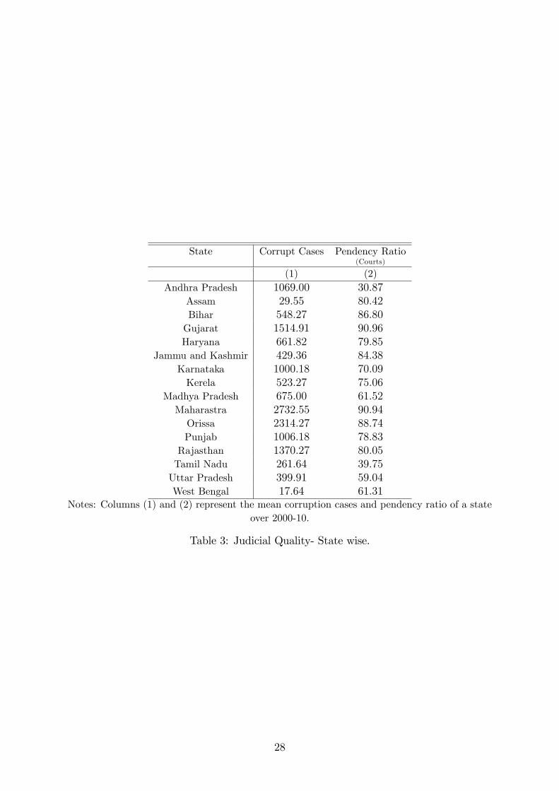
State Corrupt Cases Pendency Ratio(Courts)

(1) (2)Andhra Pradesh 1069.00 30.87

Assam 29.55 80.42Bihar 548.27 86.80Gujarat 1514.91 90.96Haryana 661.82 79.85

Jammu and Kashmir 429.36 84.38Karnataka 1000.18 70.09Kerela 523.27 75.06

Madhya Pradesh 675.00 61.52Maharastra 2732.55 90.94Orissa 2314.27 88.74Punjab 1006.18 78.83Rajasthan 1370.27 80.05Tamil Nadu 261.64 39.75Uttar Pradesh 399.91 59.04West Bengal 17.64 61.31

Notes: Columns (1) and (2) represent the mean corruption cases and pendency ratio of a stateover 2000-10.

Table 3: Judicial Quality- State wise.

28

Exports

TotalSales

TotalTrade

(1)

(2)

(3)

(4)

(5)

(6)

(7)

(8)

(9)

JudQua*InputCom

−0.

223

(0.090)b−

0.19

8(0.076)b−

0.17

7(0.075)b−

0.08

3(0.021)a−

0.09

1(0.022)a−

0.08

7(0.021)a−

0.16

0(0.067)b−

0.15

9(0.054)a−

0.15

1(0.052)b

InputComplexity

−0.

155

(0.562)

0.11

2(0.477)

0.13

3(0.467)−

0.27

3(0.129)b−

0.20

6(0.136)−

0.20

4(0.132)−

0.63

8(0.442)−

0.32

5(0.346)−

0.27

6(0.331)

JudicialQuality

0.05

4(0.026)b

0.03

3(0.023)

0.03

3(0.023)

0.00

9(0.010)

0.00

8(0.009)

0.00

9(0.009)

0.02

0(0.022)

0.00

7(0.019)

0.01

0(0.019)

FirmControls

Yes

Yes

Yes

Yes

Yes

Yes

Yes

Yes

Yes

R-square

0.01

80.

169

0.20

20.

055

0.23

50.

262

0.02

80.

193

0.22

2N

1616

916

169

1616

927

768

2776

827

768

2040

120

401

2040

1FirmFixedEffects

No

Yes

No

Yes

No

Yes

StateFixedEffects

No

Yes

Yes

No

Yes

Yes

No

Yes

Yes

YearFixedEffects

No

Yes

No

Yes

No

Yes

Firm*YearFixedEffects

No

Yes

No

Yes

No

Yes

Notes:JudicialQualityistheNoofCasesRegisteredunderCorruptionAct.Inputcomplexityistheproportionoftheintermediateinputsused

byafirm.TotalSalesisdomesticsalesplusexports.TotalTradeisexportsplusimports.Allthevariablesareexpressedintheirlogarithmform.

Firmcontrolsincludeageofafirm,agesquared,ownershipandsizeindicator.Numbersintheparenthesisareclusteredstandarderrorsatthe

firmlevel.c,b,adenotes10%,5%

and1%

levelofsignificance.Interceptsarenotreported.

Table4:BasicResults

29

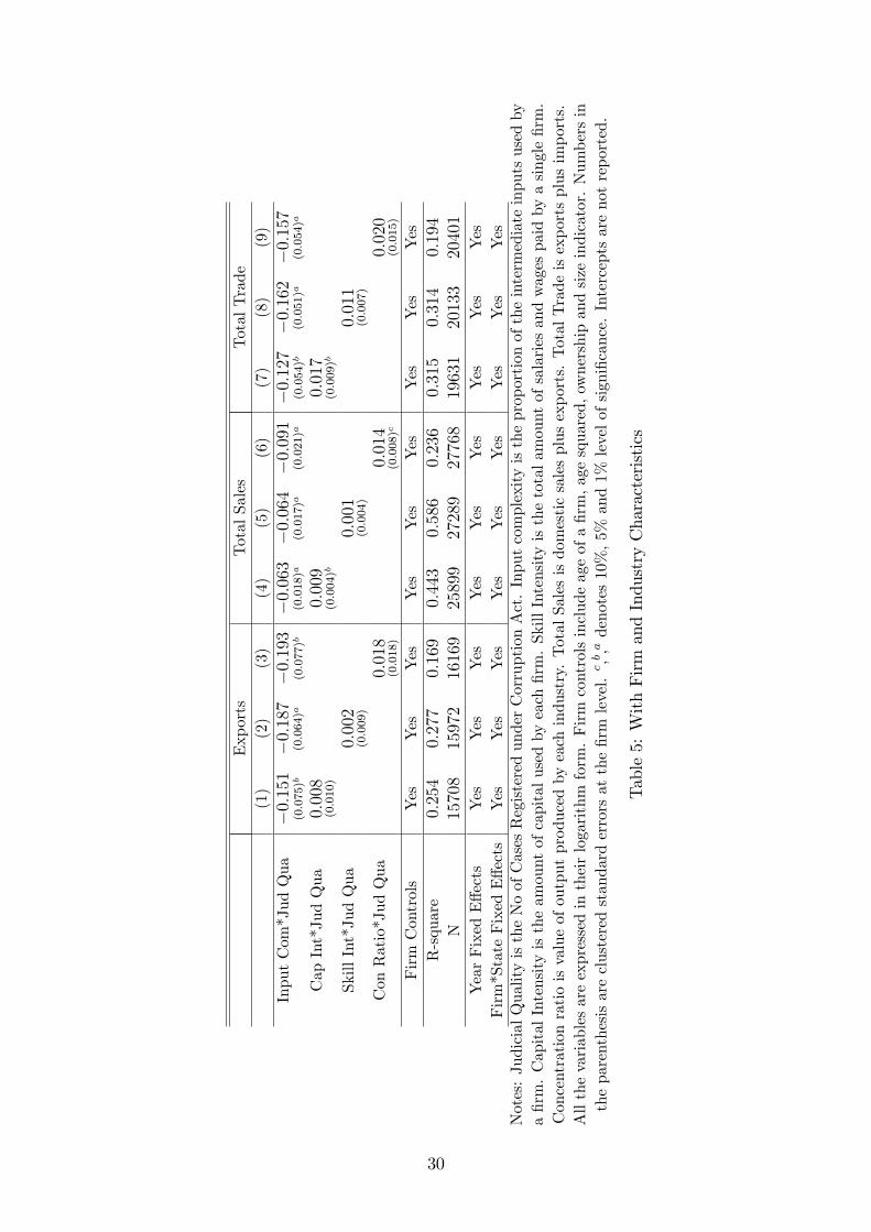
Exports

TotalSales

TotalTrade

(1)

(2)

(3)

(4)

(5)

(6)

(7)

(8)

(9)

InputCom*JudQua

−0.

151

(0.075)b−

0.18

7(0.064)a−

0.19

3(0.077)b−

0.06

3(0.018)a−

0.06

4(0.017)a−

0.09

1(0.021)a−

0.12

7(0.054)b−

0.16

2(0.051)a−

0.15

7(0.054)a

CapInt*JudQua

0.00

8(0.010)

0.00

9(0.004)b

0.01

7(0.009)b

SkillInt*JudQua

0.00

2(0.009)

0.00

1(0.004)

0.01

1(0.007)

ConRatio*JudQua

0.01

8(0.018)

0.01

4(0.008)c

0.02

0(0.015)

FirmControls

Yes

Yes

Yes

Yes

Yes

Yes

Yes

Yes

Yes

R-square

0.25

40.

277

0.16

90.

443

0.58

60.

236

0.31

50.

314

0.19

4N

1570

815

972

1616

925

899

2728

927

768

1963

120

133

2040

1YearFixedEffects

Yes

Yes

Yes

Yes

Yes

Yes

Yes

Yes

Yes

Firm*StateFixedEffects

Yes

Yes

Yes

Yes

Yes

Yes

Yes

Yes

Yes

Notes:JudicialQualityistheNoofCasesRegisteredunderCorruptionAct.Inputcomplexityistheproportionoftheintermediateinputsusedby

afirm.CapitalIntensityistheamountofcapitalusedbyeachfirm.SkillIntensityisthetotalamountofsalariesandwagespaidbyasinglefirm.

Concentrationratioisvalueofoutputproducedbyeachindustry.TotalSalesisdomesticsalesplusexports.TotalTradeisexportsplusimports.

Allthevariablesareexpressedintheirlogarithmform.Firmcontrolsincludeageofafirm,agesquared,ownershipandsizeindicator.Numbersin

theparenthesisareclusteredstandarderrorsatthefirmlevel.c,b,adenotes10%,5%

and1%

levelofsignificance.Interceptsarenotreported.

Table5:WithFirmandIndustryCharacteristics

30

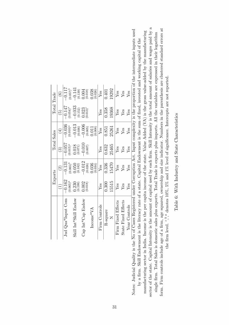
Exports

TotalSales

TotalTrade

(1)

(2)

(3)

(4)

(5)

(6)

JudQua*InputCom

−0.

162

(0.065)b−

0.13

1(0.065)b−

0.05

7(0.015)a−

0.03

6(0.010)a−

0.14

7(0.054)a−

0.11

7(0.057)b

SkillInt*SkillEndow

0.23

0(0.199)

0.05

0(0.182)

0.01

8(0.071)−

0.01

3(0.036)−

0.03

3(0.152)−

0.14

1(0.139)

CapInt*CapEndow

0.00

2(0.018)−

0.01

2(0.026)−

0.01

0(0.007)−

0.00

6(0.005)

0.02

3(0.013)c

0.00

4(0.018)

Income*VA

0.03

6(0.034)

0.01

1(0.008)

0.03

8(0.026)

FirmControls

Yes

Yes

Yes

Yes

Yes

Yes

R-square

0.30

00.

336

0.63

20.

851

0.35

80.

401

N15

515

1547

025

465

2526

119

368

1929

2FirmFixedEffects

Yes

Yes

Yes

Yes

Yes

Yes

StateFixedEffects

Yes

Yes

Yes

Yes

Yes

Yes

YearControls

Yes

Yes

Yes

Yes

Yes

Yes

Notes:JudicialQualityistheNoofCasesRegisteredunderCorruptionAct.Inputcomplexityistheproportionoftheintermediateinputsused

byafirm.SkillEndowmentistheliteracyrateofastate.CapitalEndowmentisthesumoffixed,investedandworkingcapitalofthe

manufacturingsectorinIndia.Incomeisthepercapitaincomeofthestate.ValueAdded(VA)isthegrossvalue-addedbythemanufacturing

sectorofthestate.CapitalIntensityistheamountofcapitalusedbyeachfirm.SkillIntensityisthetotalamountofsalariesandwagespaidbya

singlefirm.TotalSalesisdomesticsalesplusexports.TotalTradeisexportsplusimports.Allthevariablesareexpressedintheirlogarithm

form.Firmcontrolsincludeageofafirm,agesquared,ownershipandsizeindicator.Numbersintheparenthesisareclusteredstandarderrorsat

thefirmlevel.c,b,adenotes10%,5%

and1%

levelofsignificance.Interceptsarenotreported.

Table6:WithIndustryandStateCharacteristics

31

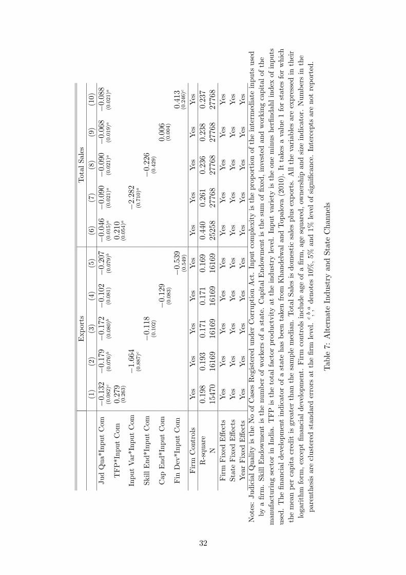
Exports

TotalSales

(1)

(2)

(3)

(4)

(5)

(6)

(7)

(8)

(9)

(10)

JudQua*InputCom

−0.

132

(0.082)c−

0.17

9(0.076)b−

0.17

2(0.080)b−

0.10

2(0.081)−

0.20

7(0.079)b−

0.04

6(0.015)a−

0.09

0(0.021)a−

0.09

0(0.021)a−

0.06

8(0.019)a−

0.08

8(0.021)a

TFP*InputCom

0.27

9(0.263)

0.21

0(0.054)a

InputVar*InputCom

−1.

664

(0.887)c

−2.

282

(0.710)a

SkillEnd*InputCom

−0.

118

(0.102)

−0.

226

(0.429)

CapEnd*InputCom

−0.

129

(0.083)

0.00

6(0.004)

FinDev*InputCom

−0.

539

(0.549)

0.41

3(0.246)c

FirmControls

Yes

Yes

Yes

Yes

Yes

Yes

Yes

Yes

Yes

Yes

R-square

0.19

80.

193

0.17

10.

171

0.16

90.

440

0.26

10.

236

0.23

80.

237

N15

470

1616

916

169

1616

916

169

2525

827

768

2776

827

768

2776

8FirmFixedEffects

Yes

Yes

Yes

Yes

Yes

Yes

Yes

Yes

Yes

Yes

StateFixedEffects

Yes

Yes

Yes

Yes

Yes

Yes

Yes

Yes

Yes

Yes

YearFixedEffects

Yes

Yes

Yes

Yes

Yes

Yes

Yes

Yes

Yes

Yes

Notes:JudicialQualityistheNoofCasesRegisteredunderCorruptionAct.Inputcomplexityistheproportionoftheintermediateinputsused

byafirm.SkillEndowmentisthenumberofworkersofastate.CapitalEndowmentisthesumoffixed,investedandworkingcapitalofthe

manufacturingsectorinIndia.TFPisthetotalfactorproductvityattheindustrylevel.Inputvarietyistheoneminusherfindahlindexofinputs

used.Thefinancialdevelopmentindicatorofastatehasbeentakenfrom

KhandelwalandTopalova(2010).Ittakesavalue1forstatesforwhich

themeanpercapitacreditisgreaterthanthesamplemedian.TotalSalesisdomesticsalesplusexports.Allthevariablesareexpressedintheir

logarithmform,exceptfinancialdevelopment.Firmcontrolsincludeageofafirm,agesquared,ownershipandsizeindicator.Numbersinthe

parenthesisareclusteredstandarderrorsatthefirmlevel.c,b,adenotes10%,5%

and1%

levelofsignificance.Interceptsarenotreported.

Table7:AlternateIndustryandStateChannels

32

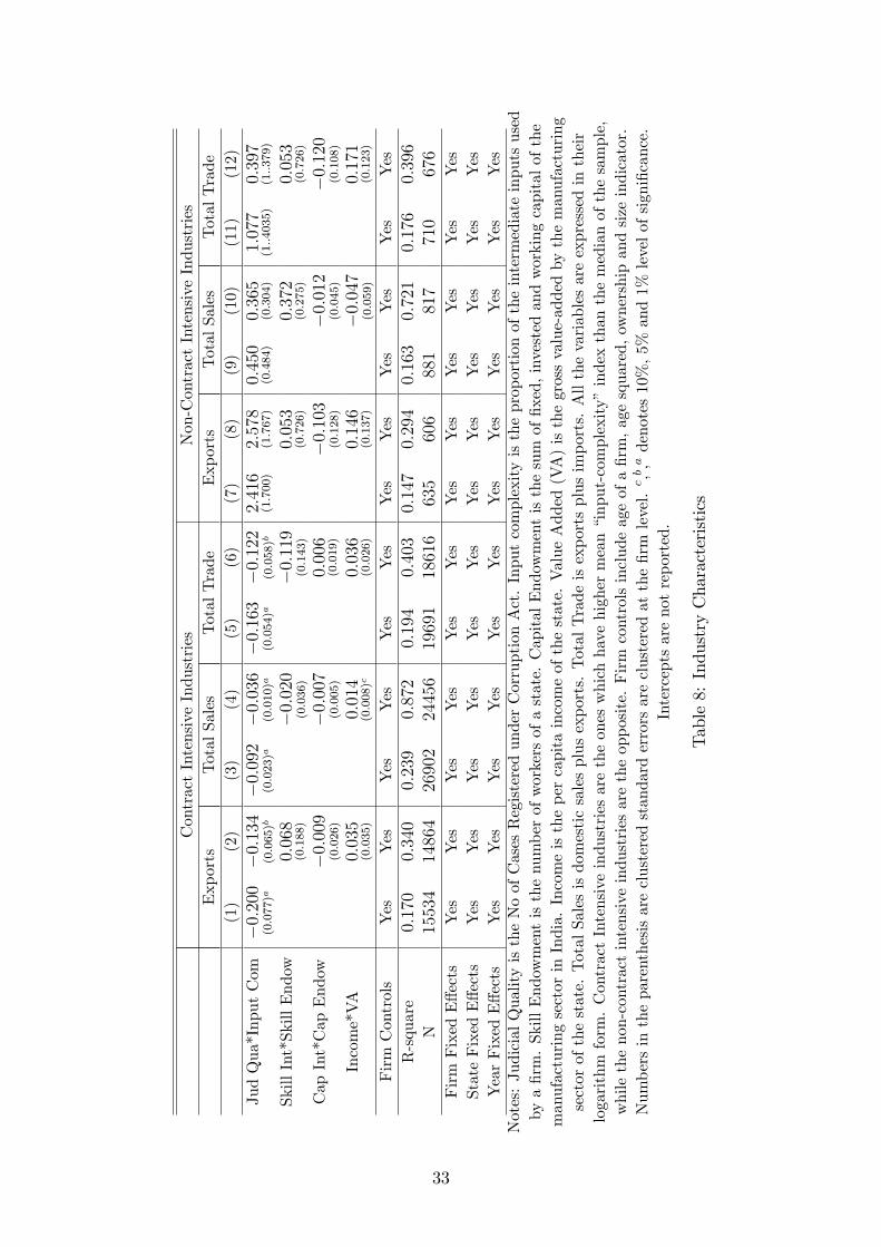
ContractIntensiveIndustries

Non-ContractIntensiveIndustries

Exports

TotalSales

TotalTrade

Exports

TotalSales

TotalTrade

(1)

(2)

(3)

(4)

(5)

(6)

(7)

(8)

(9)

(10)

(11)

(12)

JudQua*InputCom

−0.

200

(0.077)a−

0.13

4(0.065)b−

0.09

2(0.023)a−

0.03

6(0.010)a−

0.16

3(0.054)a−

0.12

2(0.058)b

2.41

6(1.700)

2.57

8(1.767)

0.45

0(0.484)

0.36

5(0.304)

1.07

7(1..4035)

0.39

7(1..379)

SkillInt*SkillEndow

0.06

8(0.188)

−0.

020

(0.036)

−0.

119

(0.143)

0.05

3(0.726)

0.37

2(0.275)

0.05

3(0.726)

CapInt*CapEndow

−0.

009

(0.026)

−0.

007

(0.005)

0.00

6(0.019)

−0.

103

(0.128)

−0.

012

(0.045)

−0.

120

(0.108)

Income*VA

0.03

5(0.035)

0.01

4(0.008)c

0.03

6(0.026)

0.14

6(0.137)

−0.

047

(0.059)

0.17

1(0.123)

FirmControls

Yes

Yes

Yes

Yes

Yes

Yes

Yes

Yes

Yes

Yes

Yes

Yes

R-square

0.17

00.

340

0.23

90.

872

0.19

40.

403

0.14

70.

294

0.16

30.

721

0.17

60.

396

N15

534

1486

426

902

2445

619

691

1861

663

560

688

181

771

067

6FirmFixedEffects

Yes

Yes

Yes

Yes

Yes

Yes

Yes

Yes

Yes

Yes

Yes

Yes

StateFixedEffects

Yes

Yes

Yes

Yes

Yes

Yes

Yes

Yes

Yes

Yes

Yes

Yes

YearFixedEffects

Yes

Yes

Yes

Yes

Yes

Yes

Yes

Yes

Yes

Yes

Yes

Yes

Notes:JudicialQualityistheNoofCasesRegisteredunderCorruptionAct.Inputcomplexityistheproportionoftheintermediateinputsused

byafirm.SkillEndowmentisthenumberofworkersofastate.CapitalEndowmentisthesumoffixed,investedandworkingcapitalofthe

manufacturingsectorinIndia.Incomeisthepercapitaincomeofthestate.ValueAdded(VA)isthegrossvalue-addedbythemanufacturing

sectorofthestate.TotalSalesisdomesticsalesplusexports.TotalTradeisexportsplusimports.Allthevariablesareexpressedintheir

logarithmform.ContractIntensiveindustriesaretheoneswhichhavehighermean“input-complexity”indexthanthemedianofthesample,

whilethenon-contractintensiveindustriesaretheopposite.Firmcontrolsincludeageofafirm,agesquared,ownershipandsizeindicator.

Numbersintheparenthesisareclusteredstandarderrorsareclusteredatthefirmlevel.c,b,adenotes10%,5%

and1%

levelofsignificance.

Interceptsarenotreported.

Table8:IndustryCharacteristics

33

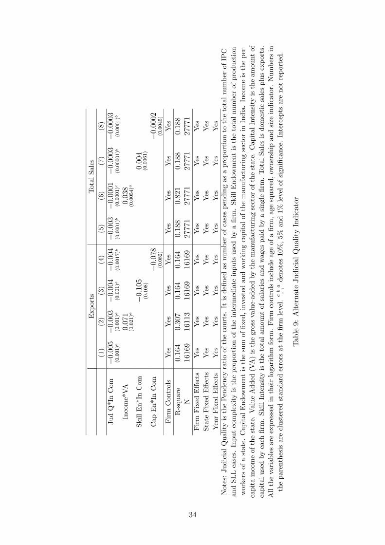
Exports

TotalSales

(1)

(2)

(3)

(4)

(5)

(6)

(7)

(8)

JudQ*InCom

−0.

005

(0.001)a−

0.00

3(0.001)a−

0.00

4(0.001)a−

0.00

4(0.0017)b−

0.00

3(0.0001)b−

0.00

01(0.0001)c−

0.00

03(0.00001)b−

0.00

03(0.0001)b

Income*VA

0.07

1(0.021)a

0.03

8(0.0054)a

SkillEn*InCom

−0.

105

(0.108)

0.00

4(0.0061)

CapEn*InCom

−0.

078

(0.082)

−0.

0002

(0.0045)

FirmControls

Yes

Yes

Yes

Yes

Yes

Yes

Yes

Yes

R-square

0.16

40.

307

0.16

40.

164

0.18

80.

821

0.18

80.

188

N16

169

1611

316

169

1616

927

771

2777

127

771

2777

1FirmFixedEffects

Yes

Yes

Yes

Yes

Yes

Yes

Yes

Yes

StateFixedEffects

Yes

Yes

Yes

Yes

Yes

Yes

Yes

Yes

YearFixedEffects

Yes

Yes

Yes

Yes

Yes

Yes

Yes

Yes

Notes:JudicialQualityisthePendencyratioofthecourts.ItisdefinedasnumberofcasespendingasaproportiontothetotalnumberofIPC

andSLLcases.Inputcomplexityistheproportionoftheintermediateinputsusedbyafirm.SkillEndowmentisthetotalnumberofproduction

workersofastate.CapitalEndowmentisthesumoffixed,investedandworkingcapitalofthemanufacturingsectorinIndia.Incomeistheper

capitaincomeofthestate.ValueAdded(VA)isthegrossvalue-addedbythemanufacturingsectorofthestate.CapitalIntensityistheamountof

capitalusedbyeachfirm.SkillIntensityisthetotalamountofsalariesandwagespaidbyasinglefirm.TotalSalesisdomesticsalesplusexports.

Allthevariablesareexpressedintheirlogarithmform.Firmcontrolsincludeageofafirm,agesquared,ownershipandsizeindicator.Numbersin

theparenthesisareclusteredstandarderrorsatthefirmlevel.c,b,adenotes10%,5%

and1%

levelofsignificance.Interceptsarenotreported.

Table9:AlternateJudicialQualityIndicator

34

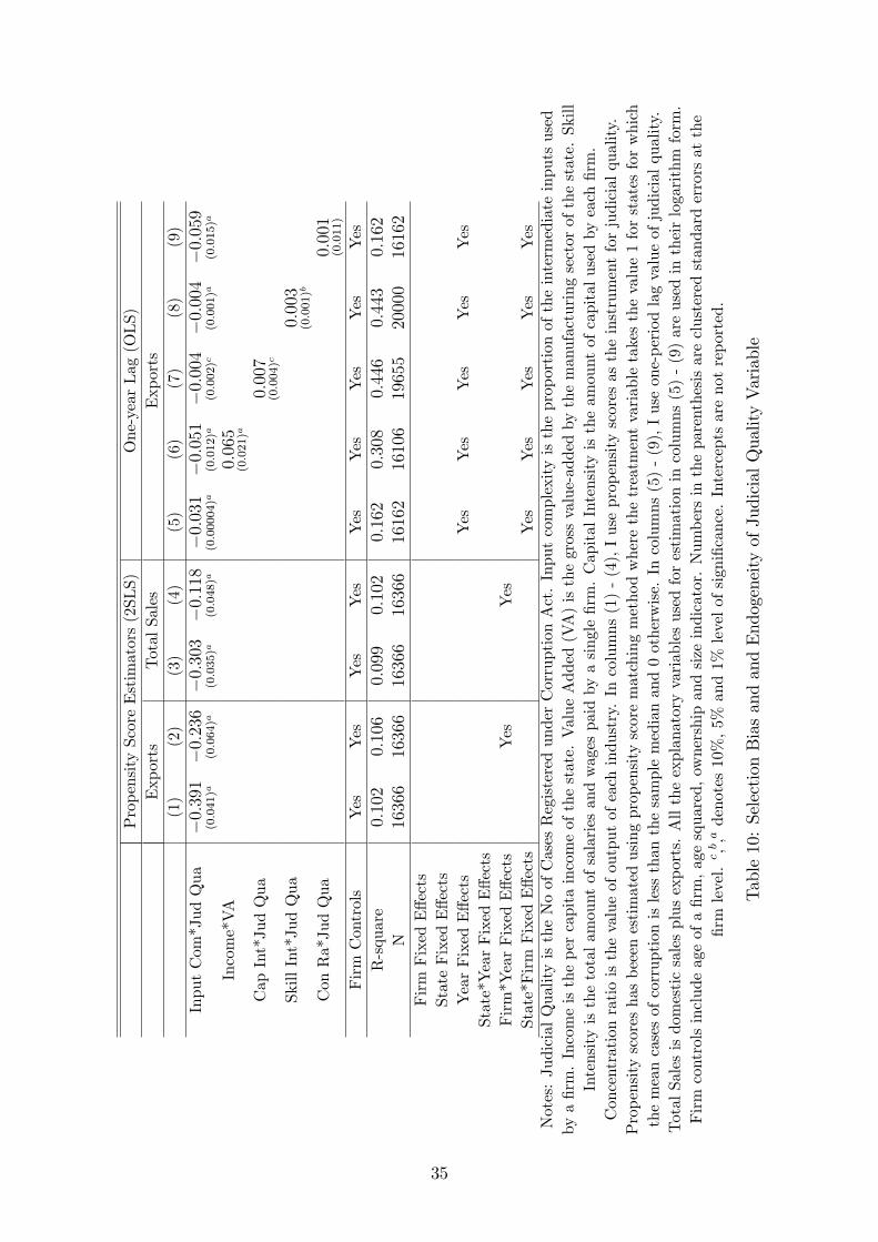
PropensityScoreEstimators(2SLS)

One-yearLag(OLS)

Exports

TotalSales

Exports

(1)

(2)

(3)

(4)

(5)

(6)

(7)

(8)

(9)

InputCom*JudQua

−0.

391

(0.041)a−

0.23

6(0.064)a−

0.30

3(0.035)a−

0.11

8(0.048)a

−0.

031

(0.00004)a−

0.05

1(0.012)a−

0.00

4(0.002)c−

0.00

4(0.001)a−

0.05

9(0.015)a

Income*VA

0.06

5(0.021)a

CapInt*JudQua

0.00

7(0.004)c

SkillInt*JudQua

0.00

3(0.001)b

ConRa*JudQua

0.00

1(0.011)

FirmControls

Yes

Yes

Yes

Yes

Yes

Yes

Yes

Yes

Yes

R-square

0.10

20.

106

0.09

90.

102

0.16

20.

308

0.44

60.

443

0.16

2N

1636

616

366

1636

616

366

1616

216

106

1965

520

000

1616

2FirmFixedEffects

StateFixedEffects

YearFixedEffects

Yes

Yes

Yes

Yes

Yes

State*YearFixedEffects

Firm*YearFixedEffects

Yes

Yes

State*FirmFixedEffects

Yes

Yes

Yes

Yes

Yes

Notes:JudicialQualityistheNoofCasesRegisteredunderCorruptionAct.Inputcomplexityistheproportionoftheintermediateinputsused

byafirm.Incomeisthepercapitaincomeofthestate.ValueAdded(VA)isthegrossvalue-addedbythemanufacturingsectorofthestate.Skill

Intensityisthetotalamountofsalariesandwagespaidbyasinglefirm.CapitalIntensityistheamountofcapitalusedbyeachfirm.

Concentrationratioisthevalueofoutputofeachindustry.Incolumns(1)-(4),Iusepropensityscoresastheinstrumentforjudicialquality.

Propensityscoreshasbeeenestimatedusingpropensityscorematchingmethodwherethetreatmentvariabletakesthevalue1forstatesforwhich

themeancasesofcorruptionislessthanthesamplemedianand0otherwise.Incolumns(5)-(9),Iuseone-periodlagvalueofjudicialquality.

TotalSalesisdomesticsalesplusexports.Alltheexplanatoryvariablesusedforestimationincolumns(5)-(9)areusedintheirlogarithmform.

Firmcontrolsincludeageofafirm,agesquared,ownershipandsizeindicator.Numbersintheparenthesisareclusteredstandarderrorsatthe

firmlevel.c,b,adenotes10%,5%

and1%

levelofsignificance.Interceptsarenotreported.

Table10:SelectionBiasandandEndogeneityofJudicialQualityVariable

35

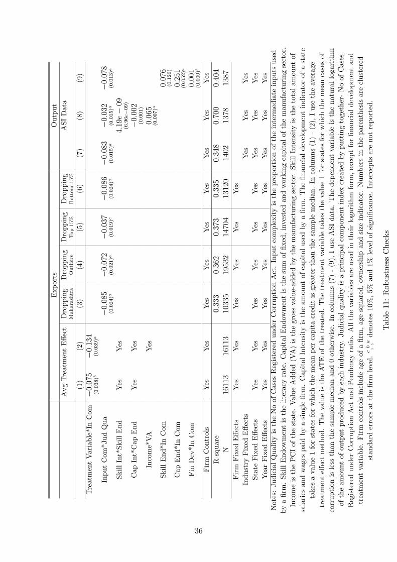
Exports

Output

AvgTreatmentEffect

Dropping

Maharashtra

Dropping

Outliers

Dropping

Top15%

Dropping

Bottom15%

ASIData

(1)

(2)

(3)

(4)

(5)

(6)

(7)

(8)

(9)

TreatmentVariable*InCom

−0.

075

(0.038)b

−0.

134

(0.039)a

InputCom*JudQua

−0.

085

(0.024)a

−0.

072

(0.021)a

−0.

037

(0.019)c

−0.

086

(0.024)a

−0.

083

(0.015)a

−0.

032

(0.015)a

−0.

078

(0.013)a

SkillInt*SkillEnd

Yes

Yes

4.19e−

09(6.96e−09)

CapInt*CapEnd

Yes

Yes

−0.

002

(0.001)

Income*VA

Yes

0.06

5(0.007)a

SkillEnd*InCom

0.07

6(0.126)

CapEnd*InCom

0.25

1(0.052)a

FinDev*InCom

0.00

1(0.000)b

FirmControls

Yes

Yes

Yes

Yes

Yes

Yes

Yes

Yes

Yes

R-square

0.33

30.

362

0.37

30.

335

0.34

80.

700

0.40

4N

1611

316

113

1033

519

532

1470

413

120

1402

1378

1387

FirmFixedEffects

Yes

Yes

Yes

Yes

Yes

Yes

IndustryFixedEffects

Yes

Yes

Yes

StateFixedEffects

Yes

Yes

Yes

Yes

Yes

Yes

Yes

Yes

Yes

YearFixedEffects

Yes

Yes

Yes

Yes

Yes

Yes

Yes

Yes

Yes

Notes:JudicialQualityistheNoofCasesRegisteredunderCorruptionAct.Inputcomplexityistheproportionoftheintermediateinputsused

byafirm.SkillEndowmentistheliteracyrate.CapitalEndowmentisthesumoffixed,investedandworkingcapitalofthemanufacturingsector.

IncomeisthePCIofthestate.ValueAdded(VA)isthegrossvalue-addedbythemanufacturingsector.SkillIntensityisthetotalamountof

salariesandwagespaidbyasinglefirm.CapitalIntensityistheamountofcapitalusedbyafirm.Thefinancialdevelopmentindicatorofastate

takesavalue1forstatesforwhichthemeanpercapitacreditisgreaterthanthesamplemedian.Incolumns(1)-(2),Iusetheaverage

treatmenteffectmethod.ThevalueistheATEofthetreated.Thetreatmentvariabletakesthevalue1forstatesforwhichthemeancasesof

corruptionislessthanthesamplemedianand0otherwise.Incolumns(7)-(9),IuseASIdata.Thedependentvariableisthenaturallogarithm

oftheamountofoutputproducedbyeachindustry.Judicialqualityisaprincipalcomponentindexcreatedbyputtingtogether-NoofCases

RegisteredunderCorruptionActandPendencyratio.Allthevariablesareusedintheirlogarithmform,exceptforfinancialdevelopmentand

treatmentvariable.Firmcontrolsincludeageofafirm,agesquared,ownershipandsizeindicator.Numbersintheparenthesisareclustered

standarderrorsatthefirmlevel.c,b,adenotes10%,5%

and1%

levelofsignificance.Interceptsarenotreported.

Table11:RobustnessChecks

36