Embed Size (px)
Citation preview

Lecture Notes in Geosystems Mathematicsand Computing
Juan Enrique SantosPatricia Mercedes Gauzellino
Numerical Simulation in Applied Geophysics

Lecture Notes in Geosystems Mathematicsand Computing
Series Editors
W. Freeden, Kaiserslautern
O. Scherzer, Vienna Z. Nashed, Orlando

More information about this series at http://www.springer.com/series/15481

Numerical Simulation in Applied Geophysics
Juan Enrique Santos • Patricia Mercedes Gauzellino

Lecture Notes in Geosystems Mathematics and Computing ISBN 978-3-319-48456-3 ISBN 978-3-319-48457-0 (eBook)DOI 10.1007/978-3-319-48457-0
© Springer International Publishing AG 2016 This work is subject to copyright. All rights are reserved by the Publisher, whether the whole or part of the material is concerned, specifically the rights of translation, reprinting, reuse of illustrations, recitation, broadcasting, reproduction on microfilms or in any other physical way, and transmission or information storage and retrieval, electronic adaptation, computer software, or by similar or dissimilar methodology now known or hereafter developed. The use of general descriptive names, registered names, trademarks, service marks, etc. in this publication does not imply, even in the absence of a specific statement, that such names are exempt from the relevant protective laws and regulations and therefore free for general use. The publisher, the authors and the editors are safe to assume that the advice and information in this book are believed to be true and accurate at the date of publication. Neither the publisher nor the authors or the editors give a warranty, express or implied, with respect to the material contained herein or for any errors or omissions that may have been made. Printed on acid-free paper This book is published under the trade name Birkhäuser, www.birkhauser-science.com The registered company is Springer International Publishing AG The registered company address is: Gewerbestrasse 11, 6330 Cham, Switzerland
Library of Congress Control Number: 2016961355
Juan Enrique Santos Patricia Gauzellino Departamento de Geofísica Aplicada Facultad de Ciencias Astronómicas y
Geofísicas UNLP Universidad Nacional de La Plata La Plata, Argentina
Mercedes Universidad de Buenos Aires
Instituto del Gas y del Petróleo Ciudad Autónoma de Buenos Aires,
Universidad Nacional de La Plata La Plata, Argentina Department of Mathematics Purdue University West Lafayette, Indiana, USA
Facultad de Ingeniería
Argentina

Juan E. Santos wish to dedicate this book tohis wife Patricia Ruberto, for her continuoussupport to the effort of writing this book.
Patricia M. Gauzellino dedicates this bookto her husband Pablo Montaner for hisconstant encouragement while writing thisbook.
Preface
Numerical simulation of waves is a subject of interest in geophysics, with applica-tions in hydrocarbon exploration and production, soil physics and non-destructivetesting of materials among others. The development of fast computational tools andalgorithms allows to represent complex models of the materials where waves aresimulated to propagate.
Wavelengths in the seismic range of frequencies are on the order of tens or hun-dreds of meters, the macro-scale, while heterogeneities in the fluid and petrophysicalproperties are on the order of centimeters, the meso-scale. This book gives a pro-cedure to include at the macro-scale the attenuation and dispersion effects sufferedby seismic waves at the meso-scale, summarizing many of the original works of theauthors on the subject.
Seismic waves in the subsurface propagate in fluid-saturated poroviscoelasticsolids, and their seismic response depends on the type of fluids, the presence offractures and microcraks and the petrophysical properties of the formations. For ex-ample, the presence of aligned fractures exhibits the medium as anisotropic at themacro-scale.
Attenuation and dispersion effects observed in seismic waves at the macro-scalescale can be explained by induced fluid flow and energy transfer between wavemodes at mesoscopic scale heterogeneities in the fluid and petrophysical properties.
First the equations describing the propagation of waves in a poroelastic matrixsaturated by a single-phase fluid, i.e., the classical Biot theory, are derived in detail.
Next, Biot theory is extended to the cases where the poroelastic matrix is satu-rated by two-phase and three-phase fluids. The case when the solid matrix is com-posed of two weakly coupled solids is also analyzed, including a procedure to deter-mine the model coefficients for shaley sandstones and partially frozen porous media.In all cases, a plane wave analysis is performed to determine the different modes ofpropagation, as well as examples illustrating the characteristics of each wave mode.
The finite element method is used to simulate the response of these types ofmulti-phase systems at the meso-scale and macro-scale. The book introduces thebasic concepts of the method, like weak solutions, variational formulation of bound-ary value problems, and defines the finite element spaces to be used to represent the
vii

viii Preface
solid and fluid displacement vectors in 1-D, 2-D and 3-D wave propagation prob-lems.
In the context of Numerical Rock Physics, this book presents several finite el-ement up-scaling procedures, formulated in the space-frequency domain, to deter-mine a long-wave equivalent viscoelastic medium to a Biot medium with multiscaleheterogeneities in the fluid and solid properties. These up-scaling procedures yieldthe complex and frequency dependent stiffness coefficients defining the viscoelasticmodel to be used to simulate wave propagation at the macro-scale.
The cases of patchy gas-brine saturation and a poroelastic matrix composed ofa fractal shale-limestone mixture are used to construct the corresponding equiva-lent isotropic viscoelastic medium. The case of a Biot medium with aligned frac-tures, modeled either as fine highly permeable and compliant layers or boundaryconditions is studied to determine an equivalent transversely isotropic viscoelasticmedium.
Wave propagation in the ultrasonic range of frequencies is illustrated for the caseof partially frozen porous media, where snapshots of the solid, ice and water phasesallow to identify all waves that can propagate in this type of medium.
The up-scaling procedures are used at the macro-scale to simulate 2-D seismicmonitoring of CO2 sequestration and 3-D wave propagation in transversely isotropicmedia. The numerical simulators are based on a finite element solution of the vis-coelastic wave equation in the space-frequency domain, with absorbing boundaryconditions at the artificial boundaries of the subsurface model, which are derivedfor elastic, viscoelastic and Biot media. Due to the large number of degrees of free-dom needed for the spatial discretization, a finite element domain decompositioniteration is used to solve the algebraic problems at a set of frequencies of interest.The time-domain solution is recovered by a discrete inverse Fourier transform.
The book is aimed at researchers and professionals working in the fields of Geo-physics, Engineering, Physics and Applied Mathematics. Basic knowledge on anal-ysis, elasticity, fluid mechanics and numerical analysis is assumed.
Buenos Aires, Juan E. SantosAugust 2016 Patricia M. Gauzellino
ix
Acknowledgements
The authors wish to thank Raul Perdomo, President of Universidad Nacional de LaPlata, for his continuous support of the research and development activities of theauthors. Besides a particular mention to Jim Douglas Jr. and M. Susana Bidner, inmemoriam. Also, the authors gratefully acknowledge the technical support receivedwhile using the computational facilities at the Facultad de Informatica of the Univer-sidad Nacional de La Plata. A special mention to Professors Charles Tritschler andPablo M. Cincotta for their continuous unconditional support. Furthermore, we areindebted to Jose M. Carcione and Gabriela B. Savioli for many discussions on thesubjects appearing in this book. Finally, thanks also to Claudia L. Ravazzoli, Ste-fano Picotti, Davide Gei, Robiel Martinez Corredor and Lucas Macias with whomthe authors have worked through the years in different scientific projects.

Contents
1 Waves in poroelastic solid saturated by a single-phase fluid . . . . . . . . 1
1.1 Biot theory . . . . . . . . . . . . . . . . . . . . . . . . . . . . . . . . . . . . . . . . . . . . . . . 11.2 Constitutive relations . . . . . . . . . . . . . . . . . . . . . . . . . . . . . . . . . . . . . . 2
1.2.1 Physical significance of the variables es and ξ . . . . . . . . . . 61.3 Determination of the elastic coefficients . . . . . . . . . . . . . . . . . . . . . . 7
1.3.1 Conditions to be satisfied by the elastic coefficients . . . . . 131.4 Inclusion of linear viscoelasticity . . . . . . . . . . . . . . . . . . . . . . . . . . . . 151.5 The equations of motion. Low frequency range . . . . . . . . . . . . . . . . 161.6 The equations of motion. High frequency range . . . . . . . . . . . . . . . . 211.7 Plane wave analysis. Attenuation and dispersion effects . . . . . . . . . 231.8 Application to a real sandstone . . . . . . . . . . . . . . . . . . . . . . . . . . . . . . 261.9 Appendix 1. Models of linear viscoelasticity . . . . . . . . . . . . . . . . . . . 29
2 A poroelastic solid saturated by two immiscible fluids . . . . . . . . . . . . . 33
2.1 Introduction . . . . . . . . . . . . . . . . . . . . . . . . . . . . . . . . . . . . . . . . . . . . . . 332.2 Constitutive relations . . . . . . . . . . . . . . . . . . . . . . . . . . . . . . . . . . . . . . 34
2.2.1 Relations to determine the two-phase elastic constants . . . 382.3 Inclusion of linear viscoelasticity . . . . . . . . . . . . . . . . . . . . . . . . . . . . 382.4 The equations of motion. Low frequency range . . . . . . . . . . . . . . . . 392.5 The equations of motion. High frequency range . . . . . . . . . . . . . . . . 412.6 Plane wave analysis . . . . . . . . . . . . . . . . . . . . . . . . . . . . . . . . . . . . . . . 432.7 Application to a real sandstone . . . . . . . . . . . . . . . . . . . . . . . . . . . . . . 44
2.7.1 Characterization of the compressional modes ofpropagation . . . . . . . . . . . . . . . . . . . . . . . . . . . . . . . . . . . . . . 45
2.7.2 Analysis of all waves in the purely elastic case . . . . . . . . . 462.7.3 Analysis of all waves as function of frequency in the
general dissipative case . . . . . . . . . . . . . . . . . . . . . . . . . . . . 48
xi

xii Contents
3 A poroelastic solid saturated by a three-phase fluid . . . . . . . . . . . . . . . 55
3.1 Introduction . . . . . . . . . . . . . . . . . . . . . . . . . . . . . . . . . . . . . . . . . . . . . . 553.2 Constitutive relations . . . . . . . . . . . . . . . . . . . . . . . . . . . . . . . . . . . . . . 563.3 The equations of motion. Low frequency range . . . . . . . . . . . . . . . . 593.4 The equations of motion. High frequency range . . . . . . . . . . . . . . . . 61
3.4.1 Phase velocities and attenuation coefficients . . . . . . . . . . . 623.5 Numerical Examples . . . . . . . . . . . . . . . . . . . . . . . . . . . . . . . . . . . . . . 65
3.5.1 Characterization of the four compressional modes ofpropagation . . . . . . . . . . . . . . . . . . . . . . . . . . . . . . . . . . . . . . 66
3.5.2 Behaviour of all waves in the purely elastic case . . . . . . . . 683.5.3 Behaviour of all waves as function of frequency . . . . . . . . 69
3.6 Appendix 1. Determination of the elastic coefficients. Inclusionof linear viscoelasticity . . . . . . . . . . . . . . . . . . . . . . . . . . . . . . . . . . . . 73
4 Waves in a fluid-saturated poroelastic matrix composed of twoweakly coupled solids . . . . . . . . . . . . . . . . . . . . . . . . . . . . . . . . . . . . . . . . 79
4.1 Introduction . . . . . . . . . . . . . . . . . . . . . . . . . . . . . . . . . . . . . . . . . . . . . . 794.2 The strain energy of the composite system . . . . . . . . . . . . . . . . . . . . 804.3 Constitutive relations . . . . . . . . . . . . . . . . . . . . . . . . . . . . . . . . . . . . . . 834.4 Determination of the coefficients in the constitutive relations . . . . . 84
4.4.1 Inclusion of linear viscoelasticity . . . . . . . . . . . . . . . . . . . . 854.5 The equations of motion . . . . . . . . . . . . . . . . . . . . . . . . . . . . . . . . . . . 86
4.5.1 Correction of the viscodynamic coefficients in the highfrequency range . . . . . . . . . . . . . . . . . . . . . . . . . . . . . . . . . . . 88
4.6 Plane wave analysis . . . . . . . . . . . . . . . . . . . . . . . . . . . . . . . . . . . . . . . 894.7 Numerical Examples. Shaley sandstones . . . . . . . . . . . . . . . . . . . . . . 904.8 Appendix 1. Calculation of the elastic coefficients in the
stress-strain relations . . . . . . . . . . . . . . . . . . . . . . . . . . . . . . . . . . . . . . 914.8.1 The case of shaley sandstones . . . . . . . . . . . . . . . . . . . . . . . 944.8.2 The case of partially frozen porous media . . . . . . . . . . . . . 944.8.3 The Kuster and Toksoz theory . . . . . . . . . . . . . . . . . . . . . . . 95
5 Absorbing boundary conditions in elastic and poroelastic media . . . . 97
5.1 The Elastic Isotropic Case . . . . . . . . . . . . . . . . . . . . . . . . . . . . . . . . . . 975.2 The case of a porous elastic solid saturated by a single-phase fluid 1075.3 The case of an isotropic porous solid saturated by a two-phase fluid5.4 The case of a composite solid matrix saturated by a single-phase
fluid . . . . . . . . . . . . . . . . . . . . . . . . . . . . . . . . . . . . . . . . . . . . . . . . . . . . 114
6 Solution of differential equations using the finite element method . . . 121
6.1 Introduction . . . . . . . . . . . . . . . . . . . . . . . . . . . . . . . . . . . . . . . . . . . . . . 1216.2 The differential model problem for 1-D wave propagation . . . . . . . 122
113

Contents xiii
6.3 A variational formulation for the 1-D wave propagation modelproblem . . . . . . . . . . . . . . . . . . . . . . . . . . . . . . . . . . . . . . . . . . . . . . . . . 124
6.4 The finite element procedure . . . . . . . . . . . . . . . . . . . . . . . . . . . . . . . . 1276.5 The algebraic problem associated with the 1-D wave propagation
model problem . . . . . . . . . . . . . . . . . . . . . . . . . . . . . . . . . . . . . . . . . . . 1306.6 A numerical example for the 1-D wave propagation problem . . . . . 1326.7 The model problem to perform harmonic experiments in 1-D
fine layered media. Backus averaging validation . . . . . . . . . . . . . . . 1346.8 Determination of the stiffness p33 . . . . . . . . . . . . . . . . . . . . . . . . . . . . 1346.9 A variational formulation for the harmonic experiment in fine
layered viscoelastic media . . . . . . . . . . . . . . . . . . . . . . . . . . . . . . . . . . 1366.10 The finite element procedure to determine the stiffness p33 . . . . . . . 1366.11 The algebraic problem associated to the harmonic experiment in
fine layered viscoelastic media . . . . . . . . . . . . . . . . . . . . . . . . . . . . . . 1376.12 A numerical example to determine the stiffness p33 . . . . . . . . . . . . . 1386.13 2-D finite element spaces . . . . . . . . . . . . . . . . . . . . . . . . . . . . . . . . . . . 139
6.13.1 Conforming finite element space over triangularpartitions of Ω to represent solid displacements . . . . . . . . 139
6.13.2 Conforming finite element space over partitions of Ωinto rectangular elements to represent solid displacements
6.13.3 Finite element spaces over rectangular an triangularmeshes to represent fluid displacements . . . . . . . . . . . . . . . 144
6.13.4 The case of a partition of Ω into rectangular elements . . . 1446.13.5 The case of a partition of Ω into triangular elements . . . . 146
6.14 3-D Finite element spaces . . . . . . . . . . . . . . . . . . . . . . . . . . . . . . . . . . 1476.14.1 Conforming finite element spaces to represent the
solid displacement using tetrahedral and 3-rectangularelements . . . . . . . . . . . . . . . . . . . . . . . . . . . . . . . . . . . . . . . . . 148
6.14.2 Finite element spaces to represent the fluiddisplacement using 3-rectangular and tetrahedralelements . . . . . . . . . . . . . . . . . . . . . . . . . . . . . . . . . . . . . . . . . 149
6.15 Non-conforming finite element spaces to represent soliddisplacements in 2-D and 3-D . . . . . . . . . . . . . . . . . . . . . . . . . . . . . . . 1506.15.1 The case of a partition of Ω into n-simplices . . . . . . . . . . . 1516.15.2 The case of a partition of Ω into n-rectangles . . . . . . . . . . 152
7 Modeling Biot media at the meso-scale using a finite elementapproach . . . . . . . . . . . . . . . . . . . . . . . . . . . . . . . . . . . . . . . . . . . . . . . . . . 155
7.1 Introduction . . . . . . . . . . . . . . . . . . . . . . . . . . . . . . . . . . . . . . . . . . . . . . 1557.2 Determination of the complex P-wave and shear moduli of the
equivalent viscoelastic medium . . . . . . . . . . . . . . . . . . . . . . . . . . . . . . 1587.3 A variational formulation . . . . . . . . . . . . . . . . . . . . . . . . . . . . . . . . . . . 1627.4 The finite element procedures . . . . . . . . . . . . . . . . . . . . . . . . . . . . . . . 163
7.4.1 Error estimates for the finite element procedures . . . . . . . . 164
142

xiv Contents
7.5 A Montecarlo approach for stochastic fractal parameterdistributions . . . . . . . . . . . . . . . . . . . . . . . . . . . . . . . . . . . . . . . . . . . . . 165
7.6 Validation of the finite element procedure . . . . . . . . . . . . . . . . . . . . . 1677.7 Analysis of the mesoscopic effects in heterogeneous Biot media . . 169
7.7.1 The patchy gas-brine saturation case . . . . . . . . . . . . . . . . . . 1697.7.2 The case of a porous matrix composed of a
shale-sandstone quasi-fractal mixture . . . . . . . . . . . . . . . . 1737.8 Application of the Montecarlo approach to determine mean
phase velocities and quality factors in Biot media with fractalheterogeneity distributions. The patchy gas-brine case . . . . . . . . . . 175
7.9 The algebraic problem associated with the determination of theplane wave modulus using the finite element procedure . . . . . . . . . 178Appendix 1. Uniqueness of the solution of the variational problems
7.11 Appendix 2. Calculation of the complex plane wave modulus ina periodic system of fluid-saturated porous layers . . . . . . . . . . . . . . 185
8 The meso-scale. Fractures as thin layers in Biot media and inducedanisotropy . . . . . . . . . . . . . . . . . . . . . . . . . . . . . . . . . . . . . . . . . . . . . . . . . 189
8.1 Introduction . . . . . . . . . . . . . . . . . . . . . . . . . . . . . . . . . . . . . . . . . . . . . . 1898.2 The Biot model and the equivalent TIV medium . . . . . . . . . . . . . . . 1918.3 Determination of the stiffnesses . . . . . . . . . . . . . . . . . . . . . . . . . . . . . 1928.4 A variational formulation . . . . . . . . . . . . . . . . . . . . . . . . . . . . . . . . . . . 194
8.4.1 Uniqueness of the solution of the variational problems . . 1978.5 The finite element method . . . . . . . . . . . . . . . . . . . . . . . . . . . . . . . . . . 1978.6 A priori error estimates . . . . . . . . . . . . . . . . . . . . . . . . . . . . . . . . . . . . 1988.7 Numerical experiments . . . . . . . . . . . . . . . . . . . . . . . . . . . . . . . . . . . . 1998.8 Appendix 1. Mesoscopic-flow attenuation theory for anisotropic
poroelastic media . . . . . . . . . . . . . . . . . . . . . . . . . . . . . . . . . . . . . . . . . 2088.9 Appendix 2. Wave velocities and quality factors .. . . . . . . . . . . . . . . 210
9 Fractures modeled as boundary conditions in Biot media andinduced anisotropy . . . . . . . . . . . . . . . . . . . . . . . . . . . . . . . . . . . . . . . . . . 213
9.1 Introduction . . . . . . . . . . . . . . . . . . . . . . . . . . . . . . . . . . . . . . . . . . . . . . 2139.2 A fractured Biot’s medium . . . . . . . . . . . . . . . . . . . . . . . . . . . . . . . . . 214
9.2.1 The boundary conditions at a fracture inside a Biotmedium . . . . . . . . . . . . . . . . . . . . . . . . . . . . . . . . . . . . . . . . . 215
9.2.2 The quasi-static experiments to determine thestiffnesses pIJ . . . . . . . . . . . . . . . . . . . . . . . . . . . . . . . . . . . . 217
9.3 A variational formulation . . . . . . . . . . . . . . . . . . . . . . . . . . . . . . . . . . 2189.4 The finite element method . . . . . . . . . . . . . . . . . . . . . . . . . . . . . . . . . 2209.5 A priori error estimates . . . . . . . . . . . . . . . . . . . . . . . . . . . . . . . . . . . . 2239.6 Numerical experiments . . . . . . . . . . . . . . . . . . . . . . . . . . . . . . . . . . . . 224
Appendix 1. Uniqueness of the solution of the variational problems
183
228
7.10
9.7

Contents xv
10 The macro-scale. Seismic monitoring of CO2 sequestration . . . . . . . . 233
10.1 Introduction . . . . . . . . . . . . . . . . . . . . . . . . . . . . . . . . . . . . . . . . . . . . . . 23310.2 The Black-Oil formulation of two-phase flow in porous media . . . . 23510.3 A viscoelastic model for wave propagation . . . . . . . . . . . . . . . . . . . . 23710.4 Continuous and discrete variational formulations for viscoelastic
wave propagation . . . . . . . . . . . . . . . . . . . . . . . . . . . . . . . . . . . . . . . . . 23910.4.1 Continuous variational formulation . . . . . . . . . . . . . . . . . . . 23910.4.2 Discrete variational formulation. The global finite
element method . . . . . . . . . . . . . . . . . . . . . . . . . . . . . . . . . . . 24010.4.3 Domain decomposition . . . . . . . . . . . . . . . . . . . . . . . . . . . . 24010.4.4 Computer implementation . . . . . . . . . . . . . . . . . . . . . . . . . . 243
10.5 Petrophysical, fluid flow and seismic data . . . . . . . . . . . . . . . . . . . . . 24610.5.1 A petrophysical model for the Utsira formation . . . . . . . . 24710.5.2 The Black Oil fluid model . . . . . . . . . . . . . . . . . . . . . . . . . . 248
10.6 Numerical simulations . . . . . . . . . . . . . . . . . . . . . . . . . . . . . . . . . . . . . 24910.6.1 CO2 injection . . . . . . . . . . . . . . . . . . . . . . . . . . . . . . . . . . . . . 251
10.7 Seismic monitoring of CO2 injection . . . . . . . . . . . . . . . . . . . . . . . . . 25210.7.1 Modeling mesoscopic-scale attenuation and dispersion
using time-harmonic experiments . . . . . . . . . . . . . . . . . . . . 25210.7.2 Time-lapse seismics applied to monitor CO2 sequestration 258
10.8 Appendix 1. IMPES solution for Black-Oil formulation . . . . . . . . . 26310.9 Appendix 2. Estimation of brine density and CO2 mole and mass
fractions in the brine phase . . . . . . . . . . . . . . . . . . . . . . . . . . . . . . . . . 266
11 Wave propagation in partially frozen porous media . . . . . . . . . . . . . . 269
11.1 Introduction . . . . . . . . . . . . . . . . . . . . . . . . . . . . . . . . . . . . . . . . . . . . . . 26911.2 The finite element domain decomposition iteration . . . . . . . . . . . . . 27011.3 A numerical example in the ultrasonic range of frequencies . . . . . . 272
12 The macro-scale. Wave propagation in transversely isotropic media 283
12.1 Introduction . . . . . . . . . . . . . . . . . . . . . . . . . . . . . . . . . . . . . . . . . . . . . . 28312.2 Properties of the equivalent TIV medium . . . . . . . . . . . . . . . . . . . . . 28412.3 The seismic modeling method . . . . . . . . . . . . . . . . . . . . . . . . . . . . . . 28712.4 Numerical experiments . . . . . . . . . . . . . . . . . . . . . . . . . . . . . . . . . . . . 29012.5 2-D seismic imaging of an anisotropic layer . . . . . . . . . . . . . . . . . . . 29412.6 Appendix 1. Rotation transformation in R3 . . . . . . . . . . . . . . . . . . . . 298
Glossary . . . . . . . . . . . . . . . . . . . . . . . . . . . . . . . . . . . . . . . . . . . . . . . . . . . . . . . . . . 301
References . . . . . . . . . . . . . . . . . . . . . . . . . . . . . . . . . . . . . . . . . . . . . . . . . . . . . . . . . 303
Chapter 1
Waves in poroelastic solid saturated by asingle-phase fluid
Abstract This chapter contains the derivation of Biot’s theory describing the prop-agation of waves in a porous elastic solid saturated by a single-phase fluid. Afterderiving the constitutive relations and the form of the potential and kinetic energydensities and the dissipation function, the lagrangian formulation of the equations ofmotion is given. Next, a plane wave analysis is performed showing the existence oftwo compressional waves and one shear wave. An example showing the behaviourof all waves as function of frequency for a sample of Nivelsteiner sandstone satu-rated by water, oil and gas is included.
1.1 Biot theory
The propagation of waves in a porous elastic solid saturated by a single–phasecompressible viscous fluid was first analyzed by Biot in several classical papers[Biot, 1956a, Biot, 1956b, Biot, 1962]. Biot assumed that the fluid may flow rel-ative to the solid frame causing friction. Biot also predicted the existence of twocompressional waves, denoted here as P1 and P2 compressional waves, and oneshear or S wave. The three waves undergo attenuation and dispersion effects fromthe seismic to the ultrasonic range of frequencies. The P1 and shear waves havea behaviour similar to those in an elastic solid, with high phase velocities, low at-tenuation and very little dispersion. At low frequencies, the P2 wave behaves as adiffusion–type wave due to its low phase velocity and very high attenuation and dis-persion, while at high frequencies becomes a truly propagating wave. The P2 wavecorresponds to motion out of phase of the solid and fluid phases while the classicP1 wave corresponds to motion in phase of the solid and fluid phases.
Biot’s theory assumes that the quantities measured at the macroscopic scale canbe described using the concepts of the continuum mechanics. In that context, thevalidity of Lagrange’s equations and the existence of macroscopic strain and kineticenergy densities and dissipation functions are assumed.
© Springer International Publishing AG 2016
in Geosystems Mathematics and Computing, DOI 10.1007/978-3-319-48457-0_1
1J.E. Santos, P.M. Gauzellino, Numerical Simulation in Applied Geophysics, Lecture Notes

2
The equations governing the macroscopic behaviour of porous media can also beobtained by means of homogenization methods, which consist on passing from themicroscopic scale description at the pore and grain scales to the mesoscopic and/ormacroscopic scale.
Contributions to the solution of this problem were given in [Sanchez Palencia, 1980]and [Bensoussan, et al., 1978], who developed the so called two-space homogeniza-tion technique. This method provides a systematic procedure for deriving macro-scopic static and dynamic equations starting from the equations governing the be-haviour of the medium at the micro-scale. It was successfully applied by differentauthors to obtain a theoretical justification of Darcy’s law and Biot’s equations ofmotion ([Levy, 1979, Burridge and Keller, 1981, Auriault et al., 1985]).
1.2 Constitutive relations
Let Ω be a porous medium saturated by a single–phase fluid, let φ(x) be the effectiveporosity, and let us,T , u f ,T be the locally averaged solid and fluid displacements inΩ . The physical meaning of u f ,T is as follows: take a unit cube Q of bulk material.Then, for any face F of the cube, the quantity∫
Fφ u f ,T ·νdF
represents the amount of fluid displaced through F , where ν denotes the unit out-ward normal to F .
Let τi j = τ i j +Δ τi j and σi j = σ i j +Δ σi j be the total stress tensor of the bulkmaterial and the stress tensor in the solid part, respectively, where Δ τi j and Δ σi j
represent changes in the corresponding stresses with respect to reference stressesτ i j and σ i j in the initial equilibrium state. Also, let p f = p f +Δ p f denote the fluidpressure, with Δ p f being the increment with respect to a reference pressure p f inthe initial equilibrium state. Also, let
σ f =−φ p f (1.1)
be the fluid pressure per unit volume of bulk material. Then,
τi j = σi j+δi jσ f = σi j−φ p f δi j, (1.2)
where δi j is the Kronecker delta.Assume that the domain Ω of bulk material with boundary denoted by ∂Ω is
originally in static equilibrium and consider a system for surface forces gθi , θ = s, f ,
where gθi represents the force in the θ−part of ∂Ω per unit surface area of bulk
material. Thus,
gsi = σ i j ν j, g fi =−φ p f δi j ν j.
1.2 Constitutive relations

1 Waves in poroelastic solid saturated by a single-phase fluid 3
Now, consider a new system of surface forces, gsi = Δσi j ν j and g fi =−φΔ p f δi j ν j,
superimposed on the original system gθi such that Ω remains in equilibrium under
the action of the total surface forces
gθ ,Ti = gθ
i +gθi , θ = s, f .
Since the fluids are at rest, all fluid pressures are constant on Ω and the total stressfield is also in equilibrium. Hence, the fluid pressure and the total stress field satisfythe conditions
∇p f =∂ p f
∂xi= 0,
∂τi j∂x j
= 0, in Ω. (1.3)
Here and in what follows the Einstein convention of sum on repeated indices is used.Let W denote the strain energy density for the fluid–solid system. Then, the
virtual work principle states that the variation of strain energy in a body Ω is equalto the virtual work of the surface forces on ∂Ω (body forces such as gravity areneglected); i.e., ∫
ΩδW dΩ =
∫∂Ω
(gsiδusi +g fi δ u f
i )d(∂Ω), (1.4)
with δusi and δ u fi being the virtual displacements.
Next, since
gsi = Δσi jν j = (Δτi j+δi jφΔ p f )ν j, g fi =−φΔ p f δi jν j, (1.5)
from (1.5) and (1.4) we obtain∫Ω
δW dΩ =
∫∂Ω
((Δτi j+δi jφΔ p f )δusiν j−φΔ p f δi jδ u fi ν j)d(∂Ω) (1.6)
=∫
∂Ω[Δτi jδusiν j−φΔ p f δi j(δ u f
i −δusi )ν j]d(∂Ω).
Set
u fi = φ(u f
i −usi ),
which represents the displacement of the fluid relative to the solid measured in termsof volume per unit area of bulk material, so that u f
i indicates the infiltration speed.Then, using Gauss’s theorem (1.6) becomes∫
ΩδW dΩ =
∫∂Ω
(Δτi jδusiν j−Δ p f δi jδu fi ν j)d(∂Ω) (1.7)
=∫
Ω
∂∂x j
(Δτi jδusi )dΩ −∫
Ω
∂∂x j
(Δ p f δi jδu fi )dΩ .

4
Next, note that since the body remains in equilibrium, using the symmetry of τi j and(1.3) we get
∂∂x j
(Δτi jδusi ) =∂Δτi j∂x j
δusi +Δτi j∂δusi∂x j
= Δτi j∂δusi∂x j
=12
Δτi j∂δusi∂x j
+12
Δτ ji∂δusi∂x j
= Δτi jδεi j(us),
where
εi j(us) =12
(∂usi∂x j
+∂usj∂xi
)denotes the strain tensor. Also,
∂∂x j
(Δ p f δi jδu fi ) =
∂Δ p f
∂xiδu f
i +Δ p f∂δu f
i
∂xi= Δ p f δ∇ ·u f .
Following Biot, we set the “increment of fluid content”
ξ =−∇ ·u f . (1.8)
Thus, (1.7) becomes∫Ω
δW dΩ =∫
Ω(Δτi jδεi j(us)+Δ p f δξ )dΩ (1.9)
Ω implies that
δW = Δτi jδεi j(us)+Δ p f δξ . (1.10)
Next, since δW must be an exact differential of the strains εi j(us) and ξ , W mustsatisfy the conditions
∂W
∂εi j= Δτi j,
∂W
∂ξ= Δ p f , (1.11)
∂ 2W
∂εi jδξ=
∂ 2W
∂ξ∂εi j,
∂ 2W
∂εi j∂εk=
∂ 2W
∂εk∂εi j. (1.12)
The strain energy density W must be invariant under orthogonal transformations.Thus, W must be a function of the linear, quadratic and cubic invariants I1, I2, andI3 of the strain tensor εi j and the scalar ξ defined in (1.8). Since we want to havea linear stress–strain relation, the I3–term must be dropped and the strain energydensity W becomes quadratic in ξ and the invariants
I1 = ε11 + ε22 + ε33 ≡ es,
I2 = ε22ε33 + ε11ε22 + ε11ε33 − ε212 − ε2
13 − ε223.
1.2 Constitutive relations
,
and the validity of (1 .9) for any

1 Waves in poroelastic solid saturated by a single-phase fluid 5
The strain energy density can be expressed in terms of the invariants separatingdilatational and deviatoric effects as well as the coupling between the solid and thefluid displacements. Also, it is convenient to use I′2 =−4I2 instead of I2:
I′
2 = 4(ε212 + ε2
13 + ε223)−4ε11ε22 −4ε22ε33 −4ε11ε33
= 2(ε212 + ε2
21 + ε213 + ε2
31 + ε223 + ε2
32)−4ε11ε22 −4ε22ε33 −4ε11ε33.
Hence, in the isotropic case,
W = W (u) =12(Eu(e
s)2 +μI′
2 −2Besξ +Mξ 2), (1.13)
where u= (us,u f ).Using (1.11) we obtain
∂W
∂ε11= Δτ11 = Eue
s+μ(−2ε33 −2ε22)−Bξ , (1.14)
∂W
∂ε22= Δτ22 = Eue
s+μ(−2ε11 −2ε33)−Bξ ,
∂W
∂ε33= Δτ33 = Eue
s+μ(−2ε22 −2ε11)−Bξ ,
∂W
∂εi j= Δτi j = 2μεi j, i = j,
∂W
∂ξ= Δ p f =−Bes+Mξ .
Next we rewrite (1.14) introducing new elastic constants and relationships amongthem. Later, the elastic constants will be determined as a function of the propertiesof the solid and fluid phases. Set
Eu = λu+2μ , λu = λ +α2 M. (1.15)
Then, from (1.14)
Δτii(u) = λues+2μεii−Bξ , i= 1,2,3;(i not summed).
Δτi j(u) = 2μεi j, i = j, Δ p f (u) =−Bes+Mξ .
In abbreviated form,
Δτi j(u) = (λues−Bξ )δi j+2μεi j, (1.16)
Δ p f (u) =−Bes+Mξ . (1.17)
In order to obtain the inverse relations for (1.16)-(1.17), it is enough to writeboth expressions in matrix form and determine the inverse matrix, resulting in thestrain-stress relations

6
Fig. 1.1 A cube of bulkmaterial.
x1
Sx1
S
1+ Δ x
εi j =1
2μΔτi j+δi j(DΔτ −FΔ p f ), (1.18)
ξ =−FΔτ +HΔ p f , (1.19)
where Δτ = Δτ11 +Δτ22 +Δτ33 = Tr(Δτ) is the trace of the tensor Δτ and D, Fand H are suitable constants.
For a better understanding of the theory, in the next paragraph we clarify themeaning of some specific variables.
1.2.1 Physical significance of the variables es and ξ
Consider a cube of bulk material as in Figure 1.1. In the initial equilibrium state,Vb,Vs, V f are the bulk, solid, and fluid volumes, respectively. Since us is the averagedsolid displacement vector over the whole bulk material, es represents the changeΔVb =Vb−Vb in bulk volume per unit volume of bulk material; i.e.,
es =ΔVbVb
.
Therefore, es denotes the volumetric strain of the bulk material. Similarly, the volu-metric strain of the pore space is defined as
ep =Vf −V f
V f=
ΔVf
V f.
The amount of fluid entering the face Sx1 is φ(u f1(x1)−us1(x1))Δx2Δx3, and the
amount of fluid leaving the face Sx1+Δx1 is φ(u f1(x1 +Δx1)−us(x1 +Δx1))Δx2Δx3.
Then, the change in fluid content δFc is given by
δFc = φ[(u f
1(x1 +Δx1)−us1(x1 +Δx1))− (u f1(x)−us1(x1))]
Δx1Δx1Δx2Δx3 ∂u f
1
∂x1Vb.
1.2 Constitutive relations

1 Waves in poroelastic solid saturated by a single-phase fluid 7
where φ =V f /Vb is the uniform porosity.In general,
δFcVb
= ∇ ·u f =−ξ .
Thus, ξ represents the change in fluid content per unit bulk volume. A positive ξvalue indicates an increase in fluid content.
Next, let us denote by ΔVcf the part of the total change ΔVf = Vf −V f in fluid
volume due to changes in fluid pressure. Then, with Cf =1Kf
denoting the fluid
compressibility,
ΔVcf
Vf=−Δ p f
Kf. (1.20)
Now observe that the change in fluid content is the difference between ΔVf andΔVc
f . Since ξ measures this difference per unit bulk volume, we see that
ξ =ΔVf −ΔVc
f
V b=
V f
Vb(ΔVf −ΔVc
f )1
V f= φ
ΔVf −ΔVcf
V f. (1.21)
Once again, ξ represents the change in fluid content.
1.3 Determination of the elastic coefficients
For the analysis that follows, we consider a cube of bulk material immersed in acontainer filled with the same fluid saturating the solid matrix. Therefore, in thebulk material the same pressure is supported by the the rock matrix and the fluid.Then, any tensional change Δτi j is conveniently decomposed into the form
Δτi j =−Δ p f δi j+Δτi j, (1.22)
where τi j is the so-called residual or effective stress of the material. Following theideas in [Santos et al., 1990a] the elastic coefficients in the right-hand side of (1.16)and (1.17) can be determined as follows. First, since the fluid does not support anyshear, μ is identical to the shear modulus of the dry matrix. To determine the re-maining coefficients in (1.16)-(1.17) it is sufficient to consider tensional changesΔτi j such that
Δτ11 = Δτ22 = Δτ33 =13
Δτ =−Δ p, Δ p> 0, Δτi j = 0, i = j.
Set13
Δτ ≡ Δτ11 = Δτ22 = Δτ33 =−Δ p.

8
Then the decomposition (1.22) become
−13
Δτ = Δ p= Δ p f +Δ p, (1.23)
and from (1.16)
13
Δτ = Δτii = (λues−Bξ )+2μεii, i not summed. (1.24)
Adding (1.24) over i we get
13
Δτ =−Δ p=
(λu+
23
μ)es−Bξ ≡ Ges−Bξ , (1.25)
Δ p f =−Bes+Mξ . (1.26)
Now, from (1.18),
εii =1
2μΔτii+(DΔτ −FΔ p f ), i not summed. (1.27)
Adding over i in (1.27),
es =
(3D+
12μ
)Δτ −3FΔ p f . (1.28)
Consider the closed system, in which no fluid is allowed to flow in or out of thebulk material, and let Ku, the bulk modulus of the undrained or closed system, bedefined by
es =−Δ pKu
. (1.29)
This corresponds to a compressibility test in which a sample of bulk material is en-closed in an impermeable jacket and then subjected to an additional external pres-sure Δ p.
Note that for a closed system ξ = 0. Then from (1.25),
es =−Δ p/G. (1.30)
Thus, from (1.29) and (1.30),
G= Ku = λu+23
μ . (1.31)
To determine Ku, we first use (1.28) to derive expressions for 3D+1
2μand F us-
ing the jacketed compressibility test [Biot and Willis, 1957], which corresponds toa tensional state such that
1.3 Determination of the elastic coefficients
Also, recall (1.19).

1 Waves in poroelastic solid saturated by a single-phase fluid 9
Δ p f = 0, es =−Δ pKm
=−Δ pKm
, (1.32)
so that the fluid pressure is held constant and the external applied pressure
−Δ p=−(Δ p f +Δ p) =−Δ p= Δτ11 = Δτ22 = Δτ33
is supported only by the solid matrix. Here Km denotes the bulk modulus of the drymatrix.
In the jacketed compressibility test, a sample of bulk material is enclosed in animpermeable jacket and immersed in a chamber filled with a fluid held at the samereference pressure p f than the fluid inside the sample. Then an additional pressurechange Δ p is applied to the fluid in the chamber. To ensure that the fluid pressure inthe sample stays at the reference value p f , a tube Tf is connected from the insideof the sample to a container filled with fluid held at the reference pressure p f . Thusthere is no change in fluid pressure as in (1.32). This test is illustrated in Figure 1.2.
Fig. 1.2 Illustration of thejacketed compressibility test.
p
p
p
p
pwpw
Tw
f
f
f
Now, using (1.20) and (1.21),
ξ =ΔVf −ΔVc
f
V b=
ΔVf
Vb=
Δ(φVb)Vb
=ΔφVb+φΔVb
Vb
=Δφ(Vb+ΔVb)+(φ +Δφ)ΔVb
Vb.
Then,
ξ Δφ +φΔVbVb
. (1.33)
Now, according to [Zimmerman et al, 1986]
Δφ =
(1Ks
− (1−φ)Km
)Δ p, (1.34)

10
where Ks denotes the bulk modulus of the solid grains. Thus, using (1.32), (1.33)and (1.34),
ξ =
(1Ks
− 1Km
)Δ p+φ
Δ pKm
+φΔVbVb
=
(1Ks
− 1Km
)Δ p. (1.35)
Now, using (1.32) in (1.28) we obtain
−Δ pKm
=
(3D+
12μ
)Δτ =
(3D+
12μ
)(Δτ11 +Δτ22 +Δτ33)
=
(3D+
12μ
)(−3Δ p).
Therefore,
3D+1
2μ=
13Km
. (1.36)
Also, from (1.19), (1Ks
− 1Km
)Δ p=−FΔτ = F 3Δ p,
so that
F =13
(1Ks
− 1Km
). (1.37)
Now using (1.29), (1.36), and (1.37) in (1.28) we obtain
es =−Δ pKu
=1
3KmΔτ −3FΔ p f =
13Km
(−3Δ p)−313
(1Ks
− 1Km
)Δ p f . (1.38)
Thus, Ku satisfies the relation
Δ pKu
=Δ pKm
+
(1Ks
− 1Km
)Δ p f . (1.39)
Next we will derive a relation between Δ p and Δ p f valid for the closed system.First note that since, for the closed system ξ = 0, from (1.12) and (1.20) we have
0 = φ(
ΔVf
V f− ΔVc
f
V f
),
so thatΔVf
V f=
ΔVcf
V f=−Δ p f
Kf. (1.40)
Next, using (1.34), up to first order terms, we have that
ΔVf
V f=
Δ(φVb)V f
= φΔVbV f
+VbV f
Δφ =Vf
Vb
ΔVbV f
+(Vb+ΔVb)
V fΔφ (1.41)
1.3 Determination of the elastic coefficients

1 Waves in poroelastic solid saturated by a single-phase fluid 11
=(V f +ΔVf )ΔVb
VbV f+
(Vb+ΔVb)ΔφV f
ΔVbVb
+Δφφ
=−Δ pKu
+1
φ
(1Ks
−(
1−φKm
))Δ p.
Combining (1.40), (1.41) and the decomposition (1.23) we see
−Δ p f
Kf=−Δ p
Ku+
1
φ
(1Ks
− (1−φ)Km
)(Δ p−Δ p f ).
Thus,
Δ p
(− 1Ku
+1
φ
(1Ks
− (1−φ)Km
))= Δ p f
(− 1Kf
+1
φ
(1Ks
− (1−φ)Km
)).
Multiplying the equation above by φ we get the relation
Δ p f =
1Ks
− 1Km
+φ(1Km
− 1Ku
)
1Ks
− 1Km
+φ(1Km
− 1Kf
)Δ p. (1.42)
Using (1.42) in (1.39) we obtain the relation
1Ku
=1Km
+
(1Ks
− 1Km
) (1Ks
− 1Km
)+φ(1Km
− 1Ku
)
(1Ks
− 1Km
)+φ(1Km
− 1Kf
). (1.43)
From (1.43), a calculation yields
Ku = KsKm+ΞKs+Ξ
, Ξ =Kf (Ks−Km)
φ(Ks−Kf ). (1.44)
We need to compute the remaining coefficients B and M. They can be obtainedfrom the jacketed compressibility test described by (1.32). From (1.25), (1.26),(1.31), and the expression for ξ in (1.35) we obtain
−Δ p=−Δ p= Ku
(−Δ pKm
)−B
(1Ks
− 1Km
)Δ p,
0 =−B
(−Δ pKm
)+M
(1Ks
− 1Km
)Δ p.
Thus,
1 =Ku
Km+B
(1Ks
− 1Km
), (1.45)

12
0 =BKm
+M
(1ks
− 1km
). (1.46)
Then using (1.44) in (1.45)
B=KsKf (Ks−Km)
Ksφ(Ks−Kf )+Kf (Ks−Km). (1.47)
Next, from (1.46),
M =K2s Kf
Ksφ(Ks−Kf )+Kf (Ks−Km). (1.48)
Note that a calculation shows that
B= α M with α = 1− Km
Ks. (1.49)
The coefficient α is known as the effective stress coefficient of the bulk material.Also, after algebraic manipulations, the coefficient M in (1.48) and the undrained
bulk modulus Ku in (1.44) can be rewritten in the form
M =
[α −φKs
+φKf
]−1
, (1.50)
Ku = Km+α2M. (1.51)
The elastic coefficients B and M can also be determined using the unjacketedcompressibility test [Biot and Willis, 1957] corresponding to a tensional state of theform
Δ p= 0, Δτ11 = Δτ22 = Δτ33 =−Δ p=−Δ p f .
In this test, a sample of bulk material is immersed in a container with the samefluid as that inside the pore space and then subjected to a hydrostatic pressure changeΔ p.
Thus, in this case, the pressure change is supported by both the solid and fluidparts of the bulk material, and the residual stress vanishes. Thus, according to (1.34),
Δφ = 0. (1.52)
Next, note that from (1.52),
ΔVsV s
=Δ((1−φ)Vb)
Vs=
(1−φ)ΔVb−ΔφVbV s
=[1− (φ +Δφ)]ΔVb
(1−φ)Vb≈ ΔVb
Vb,
ΔVf
V f=
Δ(φVb)V f
=φΔVbφVb
≈ ΔVbVb
.
.1.3 Determination of the elastic coefficients

1 Waves in poroelastic solid saturated by a single-phase fluid 13
Thus,ΔVf
V f=
ΔVsV s
=ΔVbVb
. (1.53)
SinceΔVsV s
=−Δ pKs
,
we conclude that
es =−Δ pKs
. (1.54)
Also, using (1.20), (1.21) and (1.53)
ξ = φ(
ΔVf
V f− ΔVc
f
V f
)= φ(− Δ p
Ks+
Δ p f
Kf
)= φ(
1Kf
− 1Ks
)Δ p. (1.55)
Now using (1.54) and (1.55) in (1.25)–(1.26), we obtain
1 =Ku
Ks+Bφ
(1Kf
− 1Ks
), 1 =
BKs
+Mφ(
1Kf
− 1Ks
). (1.56)
Now, from (1.56) and algebraic manipulations using the expression for Ku in (1.44)we recover the expression for B and M given in (1.47) and (1.48).
1.3.1 Conditions to be satisfied by the elastic coefficients
We now examine the restrictions on the coefficients imposed by the nonnegativecharacter of the strain energy W . First note that (1.13) can be written in the equiva-lent form
2W = Ku(es)2 +4μ(ε2
12 + ε213 + ε2
23) (1.57)
+23
μ((ε11 − ε22)
2 +(ε11 − ε33)2 +(ε22 − ε33)
2)−2Besξ +Mξ 2.
Second, consider pure shear and compression; setting
es = ξ = 0
in (1.57) we must haveμ > 0.
Next, settingε11 = ε22 = ε33, εi j = 0, i = j,
in (1.57) we obtain
2W = Ku(es)2 −2Besξ +Mξ 2

14
= (es ξ )(
Ku −B−B M
)(es
ξ
).
Thus, for W to be a positive definite quadratic form in the variables es and ξ wefind the conditions
KuM−B2 > 0, Ku > 0, M > 0.
Next, we observe that, since B= αM and λu = λ +α2M (cf. (1.15) and (1.49))
KuM−B2 = KuM−α2M2 = (Ku−α2M)M.
Next, set
K = λ +23
μ .
Then,
Ku−K = λu+23
μ −λ − 23
μ = λu−λ = α2M
so thatKuM−B2 = (Ku−α2M)M = KM.
Therefore, for W to be nonnegative, we have the necessary and sufficient conditions
μ > 0, M > 0, K = λ +23
μ > 0. (1.58)
To interpret the condition K = λ + 23 μ > 0, we proceed as follows. From (1.17):
ξ =1M
Δ p f +αes. (1.59)
Using (1.59) in (1.16) we obtain
Δτi j+δi jαΔ p f = 2μεi j+δi j(λu−α2M)es. (1.60)
Now using (1.22) in (1.60) to write the strain Δτi j in terms of the residual stressΔτi j and the fluid pressure Δ p f the following relation is obtained:
Δτi j− (1−α)δi jΔ p f = 2μεi j+δi jλes. (1.61)
Next, in the case of the jacketed compressibility test defined in (1.32) Δ p f = 0and (1.61) reduces to
−Δ p= 2μεii+λes, i not summed.
Hence,
es =− Δ p
λ + 23 μ
=−Δ pK
.
1.3 Determination of the elastic coefficients
1 Waves in poroelastic solid saturated by a single-phase fluid 15
Thus, the requirement K = λ + 23 μ > 0 in (1.58) simply states the physically mean-
ingful condition that, for the open system , the inverse of the jacketed compressibil-ity be positive.
1.4 Inclusion of linear viscoelasticity
It is well known that wave dispersion and attenuation phenomena in real saturatedrocks are higher than the associated to viscodynamic effects [Mochizuki, 1982,Stoll and Bryan, 1970, Carcione, 2014]. This is mainly due to the complexity ofpore shapes, heterogeneities in the physical properties and in the distribution of thefluids and the intrinsic anelasticity of the frame. These factors can be included inthe formulation by means of the theory of viscoelasticity. The theoretical basis forthis generalization was given by Biot (1956a,1962), who developed the general the-ory of deformation of porous materials saturated by viscous fluids when the solidphase exhibits linear viscoelastic behaviour. Using principles of irreversible thermo-dynamics Biot established a general operational relationship between generalizedforces Qi and observed coordinates qi, of the form
Qi = Ti jq j,
where Ti j is a symmetric matrix. In this way Biot obtained a general correspon-dence rule between the elastic and viscoelastic formulations in the domain of theLaplace transform and showed that formally all the relations are identical. The poro-viscoelastic formulation obtained in this way was later applied by different authorsfor the study of wave propagation problems (see [Stoll and Bryan, 1970, Stoll, 1974,Keller, 1989, Rasolofosaon, 1991]).
It follows from (1.16)-(1.17) that the forces of our model are related to the vari-ables ξ and εi j by means of a symmetric matrix, whose elements are functions ofthe elastic coefficients. Thus, if we assume that the bulk material shows linear vis-coelastic behaviour, we are able to extend the constitutive relations (1.16)-(1.17)by simply replacing the real elastic moduli μ ,Ku and M by appropriate viscoelasticoperators.
Next, for any function f (t) let f (ω) indicate the Fourier transform of f (t), ωbeing the angular frequency, i.e.
f (t) =∫ ∞
∞f (ω)e−iωtdt.
Hence, using Fourier transform in time we can state in the space–frequency do-main the constitutive relations (1.16)-(1.17) as follows:
Δτi j(u(ω)) = (λu(ω)es(ω)−B(ω)ξ (ω))δi j+2μ(ω)εi j(ω),
Δ p f (u(ω)) =−B(ω)es(ω)+M(ω)ξ (ω).

16
where λu(ω),μ(ω),B(ω),M ω) are complex frequency dependent poroviscoelasticmoduli.
Models to determine these frequency dependent poroviscoelastic moduli startingfrom the corresponding poroelastic ones are given in Appendix 1.9.
1.5 The equations of motion. Low frequency range
We will choose usi and u fi , 1 ≤ i≤ 3 as generalized coordinates or state variables to
describe the evolution of the fluid–solid system. The Lagrange formulation of theequation of motion is given by
ddt
(∂Td
∂ usi
)+
∂Dd
∂ usi=−∂Vd
∂usi, (1.62)
ddt
(∂Td
∂ u fi
)+
∂Dd
∂ u fi
=−∂Vd
∂u fi
, 1 ≤ i≤ 3. (1.63)
In (1.62)-(1.63) Td , Dd , and Vd are, respectively, the kinetic energy density, thedissipation energy density function, and the potential energy density of the system.
First, let us compute the right hand side in (1.62)-(1.63). Let
V =
∫Ω
W dΩ −∫
∂Ω(gsi u
si +g f
i ufi )d(∂Ω)
be the potential energy of the fluid–solid system where gsi ,gfi are given in (1.5).
Now we consider a perturbation of the system from the equilibrium state; i.e.,the conditions (1.3) do not hold anymore. Then, using the argument leading to (1.7)and the relation (1.10) we get
δV =∫
ΩδW dΩ −
∫∂Ω
((Δτi j+φΔ p f δi j)δusiν j−φΔ p f δi jδ u fi ν j)d(∂Ω)
=∫
ΩδW dΩ −
∫∂Ω
(Δτi jδusiν j−Δ p f δi jδu fi ν j)d(∂Ω) (1.64)
=∫
ΩδW dΩ −
∫Ω
∂∂x j
(Δτi jδusi )dΩ +∫
Ω
∂∂x j
(Δ p f δi jδu fi )dΩ
=∫
Ω(Δτi jδεi j+Δ p f δξ )dΩ −
∫Ω
∂Δτi j∂x j
δusi dΩ −∫
ΩΔτi jδεi jdΩ
+∫
Ω
∂Δ p f
∂xiδu f
i dΩ +∫
ΩΔ p f (−δξ )dΩ .
Hence,
δV =−∫
Ω
(∂Δτi j∂x j
δusi −∂Δ p f
∂xiδu f
i
)dΩ =
∫Ω
δVddΩ .
1.5 The equations of motion. Low frequency range
(

1 Waves in poroelastic solid saturated by a single-phase fluid 17
Thus,
δVd =−∂Δτi j∂x j
δusi +∂Δ p f
∂xiδu f
i .
Assuming that Vd is an exact differential in the variables usi and u fi , we see that
∂Vd
∂usi=−∂Δτi j
∂x j,
∂Vd
∂u fi
=∂Δ p f
∂xi, i= 1,2,3. (1.65)
Next, we will compute the kinetic energy density Td for the fluid–solid system.Let us consider a unit cube Q of bulk material, and let Qp denote the porous part ofQ. Let ρ f and ρs be the mass densities of the fluid and solid phases, respectively.
Let (vi)1≤i≤3 be the relative micro-velocity field; i.e., the velocity of each fluidparticle with respect to the solid frame. Assuming that the relative flow inside thepore space is of laminar type (i.e., we are in the low frequency range) we can write
vi = ai jufj ,
with the coefficients ai j depending on the coordinates of the pores and the poregeometry. Let
ρ1 = (1−φ)ρs
be the mass of solid per unit volume of bulk material. Then, on the solid part of Qthe kinetic energy is given by
12
∫Q\Qp
ρsusi u
si d(Q\Qp) =
12|Q\Qp|ρsu
si u
si =
12
ρ1usi u
si . (1.66)
Here we have used that since usi is the average solid displacement over Q, usi isconstant over Q. In (1.66) |Q\Qp| indicates the measure of the set Q\Qp.
Next, on the porous part Qp, the velocity of any given particle is the relativemicrovelocity plus the averaged solid velocity; i.e., usi + vi. Then the kinetic energyin Qp is obtained by integration of (usi + vi)(usi + vi) over Qp. Thus, the total kineticenergy per unit volume of bulk material is given by
Td =12
ρ1usi u
si +
12
ρ f
∫Qp
(usi + vi)(usi + vi)dQp. (1.67)
Next, note that
12
ρ f
∫Qp
usi usi dQp =
12
ρ f φ usi usi (1.68)
and that
ρ f
∫Qp
usi vidQp = ρ f usi
∫Qp
vidQp = ρ f usi u
fi , (1.69)

18
since the averaged relative fluid velocity is obtained by averaging the relative micro-velocity field over Qp.
Next,
ρ f
∫Qp
vkvkdQp = ρ f
∫Qp
akiufi ak ju
fj dQp (1.70)
=
(ρ f
∫Qp
akiak jdQp
)u fi u
fj = gi ju
fi u
fj ,
where
gi j = ρ f
∫Qp
akiak jdQp.
Note that gi j = g ji.Using (1.68), (1.69), and (1.70) in (1.67), we obtain
Td =12
ρ usi usi +ρ f usi u
fi +
12gi ju
fi u
fj , (1.71)
whereρ = ρ1 +ρ f φ = (1−φ)ρs+φρ f
is the mass density of bulk material.Note that gi j must be positive definite, otherwise, we may have, for usi ≡ 0,
T =12gi ju
fi u
fj = 0 for uf
i = 0.
For an isotropic micro-velocity field, we have that
gi j = gδi j,
and (1.71) becomes
Td =12
ρ usi usi +ρ f usi u
fi +
12gu f
i ufi . (1.72)
In order that the kinetic energy density in (1.72) be positive, the conditions
ρg−ρ2f > 0, g> 0, ρ > 0,
must be satisfied.Next, we will compute the form of the dissipation energy density function Dd .
Following [Biot, 1956a], we will assume that dissipation depends only on the rel-ative flow between the fluid and the solid. Assuming that the relative flow is ofPoiseuille type, the microscopic flow pattern inside the pores is uniquely deter-
mined by the six generalized velocities usi , ˙ufi . The dissipation function vanishes
when usi =˙ufi . Thus, we can write Dd in the form
1.5 The equations of motion. Low frequency range

1 Waves in poroelastic solid saturated by a single-phase fluid 19
Dd =12
ηri ju fi u
fj (1.73)
where η is the fluid viscosity and ri j is a symmetric positive definite matrix. Now,from (1.71) and (1.73) we have that
∂Td
∂ usk= ρ usk+ρ f u
fk ,
∂Td
∂ u fk
= ρ f usk+gk ju
fj , (1.74)
∂Dd
∂ usk= 0,
∂Dd
∂ u fk
= ηrk jufj .
Thus, combining (1.65) and (1.74) we see that the Lagrange equations (1.62)-(1.63)become
ρ usi +ρ f ufi =
∂Δτi j∂x j
, (1.75)
ρ f usi +gi ju
fi +ηri ju f
j =−∂Δ p f
∂xi, (1.76)
which are Biot’s equation of motion for the fluid–solid system.Note that in the case of steady flow rate (u f
i = const) and vanishing solid accel-erations from (1.76) we have that
ηri ju fj =
∂Δ p f
∂xi. (1.77)
Let κ = (κi j) be the inverse of the matrix R= (ri j). Then, (1.77) is Darcy’s Law
so that κ can be identified with the rock permeability.Next, in the isotropic case,
ri j = rδi j = κ−1δi j, gi j = gδi j. (1.78)
Thus, in the isotropic case, (1.75)-(1.76) become
ρ us+ρ f u f = ∇ ·Δτ(u), (1.79)
ρ f us+gu f +ηκ−1u f =−∇Δ p f (u). (1.80)
Equations (1.79)- (1.80) together with the constitutive relations given in (1.16)-(1.17) completely determines the dynamic behaviour of the solid–fluid system inthe low–frequency range.
Let us write the equations of motion (1.79)-(1.80) and the constitutive relations(1.16)-(1.17) in terms of usi , u
fi , in order to recover Biot’s equation in the original
form in [Biot, 1956a], which validity is restricted to constant porosity case. Using(1.2), from (1.79) we have
ηκ−1u f = ∇ ,p f

20
ρ usi +ρ f φ( ¨ufi − usi ) =
∂Δσi j
∂x j+
∂Δσ f
∂xi. (1.81)
Multiplying (1.80) by φ we see that
∂Δσ f
∂xi=−φ
∂Δ p f
∂xi= φρ f u
si +φgu f
i +ηκ−1φ u fi (1.82)
= φρ f usi +φ 2g( ¨u
fi − usi )+ηκ−1φ 2( ˙u
fi − usi )
= (φρ f −φ 2g)usi +φ 2g ¨ufi +ηκ−1φ 2( ˙u
fi − usi ).
Using (1.82) in (1.81), we obtain
∂Δσi j
∂x j= (ρ −2φρ f +φ 2g)usi +(φρ f −φ 2g) ¨u
fi +φ 2ηκ−1(usi − ˙u
fi ). (1.83)
Set
ρ11 = ρ −2φρ f +φ 2g, ρ12 = φρ f −φ 2g,
ρ22 = φ 2g, b= φ 2ηκ−1.
Then (1.82) and (1.83) become
ρ11us+ρ12¨uf −b( ¨u
f − us) = ∇ ·Δσ , (1.84)
ρ12us+ρ22¨uf+b( ¨u
f − us) =−φ∇Δ p f . (1.85)
Next we will give constitutive relations for Δσi j and Δσ f = −φΔ p f in terms ofεi j(us), es and θ = ∇ · u f . First, note that
ξ =−∇ ·u f =−∇ · (φ(u f −us)) = φ(es− θ).
Thus, from (1.17) and using that B= αM (see (1.49))
σ f = φM(α −φ)es+φ 2Mθ . (1.86)
Using (1.2), (1.16) and (1.86) and that λu = λ +α2 M (see (1.15)), we obtain
Δσi j = Δτi j−δi jΔσ f (1.87)
=([λ +M(α −φ)2]es+φM(α −φ)θ
)δi j+2μεi j.
SettingA= λ +M(α −φ)2, P= φ(α −φ)M, R= φ 2M, (1.88)
we can rewrite (1.85) and (1.87) in the form
1.5 The equations of motion. Low frequency range

1 Waves in poroelastic solid saturated by a single-phase fluid 21
Δσi j = (Aes+P θ)δi j+2μεi j, (1.89)
−φΔ p f = Pes+R θ . (1.90)
The coefficient α in (1.88) was shown to be in the range φ ≤ α ≤ 1 ( see[Biot and Willis, 1957] their equation [28]), so that the coefficients A,P and R arestrictly positive.
The equations of motion (1.84)- (1.85) together with the constitutive relations(1.89)-(1.90) are the original equations derived in [Biot, 1956a].
1.6 The equations of motion. High frequency range
The equations of motion (1.79)-(1.80) were derived under the assumption that theflow inside the pore space is of Poiseuille type. This assumption breaks down if thefrequency exceeds a certain critical value ωc. This occurs when inertial and viscousforces in (1.76) are of the same order, i.e., when g ω ≈ ηκ−1, so that
ωc =ηκ−1
g=
ηκ−1φρ fS
, (1.91)
where we have used that
g=Sρ f
φ,
with S being the tortuosity factor; it can be estimated as follows ([Berryman, 1981]):
S=12
(1+
1φ
). (1.92)
By analyzing the flow in cylindrical ducts and in plane slits [Biot, 1956b] con-cludes that in the high frequency range the equations of motion (1.84)-(1.85) mustbe modified employing a universal function
F(θ(ω)) =14
θ(ω)T (θ(ω))
1− 2iθ(ω)
T (θ(ω))= FR(θ(ω))+ iFI(θ(ω)),
T (θ(ω)) =ber
′(θ(ω))+ ibei
′(θ(ω))
ber(θ(ω))+ ibei(θ(ω))(1.93)
that can be adopted to represent the frequency effect with a non-dimensional param-eter
θ(ω) = ap
(ωη
) 12
where ap is the pore–size parameter depending on size and pore geometry and

22
η = η/ρ f
is the kinetic viscosity. The parameter ap can be estimated as
ap = 2(κA0/φ)12 ,
where A0 denotes the the Kozeny–Carman constant.In (1.93) ber(θ(ω)),bei(θ(ω)) are the Kelvin functions of the first kind and zero
order.Another frequency correction function was later presented by [Johnson et al., 1987]:
F(ω) =
(1− i
4S2κxΛ 2φ
); where x =
ηφκ−1
ωρ, (1.94)
and Λ can be calculated from8SκφΛ 2 = 1. (1.95)
The coefficient Λ has the dimensions of length and is a geometrical parameter ofthe porous medium.
Now we write the high–frequency form of Biot’s equations of motion (1.84)-(1.85) and constitutive equations (1.89)-(1.90) in the space–frequency domain as:
−ω2ρ11us(ω)−ω2ρ12uf (ω)− iωb F(ω)(u f (ω)−us(ω)) (1.96)
= ∇ ·Δσ ,
−ω2ρ12us(ω)−ω2ρ22u f (ω)+ iωbF(ω)(u f (ω)−us(ω)) (1.97)
=−φ∇Δ p f ,
Δσi j(us(ω), u f (ω)) = [Aes(ω)+P θ(ω)]δi j+2μεi j(us(ω)), (1.98)
−φΔ p f (us(ω), u f ) = P es(ω)+R θ(ω). (1.99)
Next, after algebraic manipulations, we can write the equations (1.96)-(1.97) us-ing the variables us(ω) and u f (ω) = φ(u f (ω)−us(ω)) as:
−ω2ρus(ω)−ω2ρ fu f (ω)−∇ ·Δτ = f(1), (1.100)
−ω2ρ fus(ω)−ω2 g(ω)u f (ω)+ iωb(ω)u f (ω)+∇Δ p f = f(2), (1.101)
where f(1) and f(2) are external forces in the bulk material and the fluid per unit bulkvolume and
g(ω) =Sρ f
φ+
FI(ω)
ωηκ−1,
b(ω) = ηκ−1FR(ω).
Equation (1.100)-(1.101) together with the constitutive relations
1.6 The equations of motion. High frequency range

1 Waves in poroelastic solid saturated by a single-phase fluid 23
Δτi j(u(ω)) = (λues−Bξ )δi j+2μεi j(us(ω)), (1.102)
Δ p f (u(ω)) =−Bes+Mξ . (1.103)
are Biot’s equations in the high-frequency range.Let us analyze the asymptotic properties of the frequency correction function
F(ω).For the function defined in (1.93),
F(θ(ω))→ 14
θ(ω)1√2(1+ i), as θ(ω)→ ∞
Also,
F(θ(ω))→ 1+ iθ(ω))2
24, as θ(ω)→ 0.
For the function in (1.94),
F(ω)→ 2κSΛφ
[−iωρ f
η
]1/2
, as ω → ∞
F(ω))→ 1 as ω → .
Thus at low frequencies the low–frequency coefficients are recovered, and at highfrequencies these correcting functions behave like ω 1
2 .Remark λu,μ and M in (1.102)-
(1.103) become complex and frequency dependent.
1.7 Plane wave analysis. Attenuation and dispersion effects
Assuming constant coefficients in the constitutive relations (1.102)-(1.103), in theabsence of external forces, (1.100)-(1.101) can be stated in the form
−ω2ρus−ω2ρ fu f = (λu+μ)∇es−B∇ξ +μ∇2us, (1.104)
−ω2ρ fus−ω2gu f + iηκ−1u f =−∇[−Bes+M ξ ]. (1.105)
Applying the divergence operator to (1.104)-(1.105) we obtain the equations gov-erning the propagation of dilatational waves:
−ω2ρ es−ω2ρ f ef = Eu ∇2 es+B ∇2 e f , (1.106)
−ω2ρ f es−ω2 ge f + iωηκ−1 e f = B∇2 es+M ∇2 e f , (1.107)
where e f = ∇ ·u f .
0
. If viscoelasticity is included, the coefficients

24
Next consider a plane compressional wave of angular frequency ω and wavenumber = r+ ii travelling in the x1–direction; i.e.,
es =C()s ei(x1−ωt) =C()
s e−ix1eir(x1− ωrt), (1.108)
e f =C()f ei(x1−ωt) =C()
f e−ix1eir(x1− ωrt). (1.109)
Substitution of (1.108)-(1.109) in (1.106)-(1.107), setting
γ =ω
and defining the matrices
A =
(ρ ρ f
ρ f g
)E =
(Eu BB M
)C γ =
(C γs
C γf
),
where
g= g+ iηκ−1
ω
leads to the following generalized eigenvalue problem:
γ2AC(γ) = EC(γ). (1.110)
Now from (1.110) it is seen that to determine the complex wave-numbers = r+ iiit is sufficient to solve the problem
det(S − γ2I) = 0, (1.111)
where
S = A−1
E .
Equation (1.111) gives two physically meaningful solutions (i.e., i>0)γ ( j))2, j=
1,2 that in turn determine two phase velocities v( j) and attenuation coefficients ( j)icorresponding to the P1 and P2 compressional modes of propagation.
Taking divergence the equations of motion (1.84)-(1.85) in terms of the solid dis-placement us and absolute fluid displacement u f Biot demonstrated that P1 wavescorresponds to motions in phase of the solid and fluid phases, while for P2 wavesthe solid and fluid phases move in opposite phase, [Biot, 1956a].
The phase velocities for compressional waves v( j) are given by
v( j) =ω
|( j)r |, j = 1,2.
1.7 Plane wave analysis. Attenuation and dispersion effects

1 Waves in poroelastic solid saturated by a single-phase fluid 25
Instead of the attenuation coefficient ()i , it is convenient to use another attenuationcoefficient defined as follows: from (1.108) and (1.109) we see that at x1 = 0, theoriginal wave amplitude amplitude for eθ ,θ = s, f , is
eθ1 =C(( j))
θ .
Since the wavelength λ ( j) of a wave travelling with speed v( j) and frequency ω is
λ ( j) =2πv( j)
ω,
after travelling one wavelength the wave has amplitude
eθ2 = eθ
0 e−
( j)i
2πv( j)ω .
Thus,
log10
(eθ
2
eθ1
)=−
( j)i
2π
( j)r
log10(e).
We define the attenuation coefficient b( j) measured in dB by the formula
b( j) =−20log10
(eθ
2
eθ1
)= (2π)(8.685889)( j)i /|( j)r |.
Hence this coefficient b( j) measures the wave attenuation after travelling one wave-length. For example, an attenuation coefficient b( j) of 20 dB implies that after trav-elling one wavelength the Pj-wave has reduced ten times its original amplitude.
Next we consider rotational waves. Let
ks = ∇×us, k f = ∇×u f .
Then applying the curl operator to equations (1.104)-(1.105) we obtain the relationsgoverning the propagation of rotational waves:
ρks+ρ fk f = μΔks, (1.112)
ρ fks+gk f + iηκ−1k f = 0. (1.113)
Let us consider a plane rotational wave of angular frequency ω and wave number= r+ ii travelling in the x1–direction:
ks =C()1 e−ix1eir(x1− ω
rt), (1.114)
k f =C()2 e−ix1eir(x1− ω
rt). (1.115)
Substitution of (1.114)-(1.115) in (1.112)-(1.113) yields
−ω2[C1ρ +C2ρ f ] =−2μC1, (1.116)

In this section we compute phase velocities and attenuation coefficients for a sampleof Nivelsteiner sandstone, a friable sandstone mainly composed of quartz with smallpercentages of rock fragments and potash-feldspar [Kelder and Smeulders, 1997].Its material properties, taken from [Arntsen and Carcione, 2001], and those of thesaturant fluids, water, oil and gas, are given in Table 1.1.
The gas properties correspond to a dry gas at a reference pressure of 5MPa, (ata depth of 500 m, approximately ) using the calculations given in [Standing, 1977]and [McCoy, 1983].
Table 1.1 Material properties of the Nivelsteiner sandstone
Solid grains bulk modulus, Ks 36. GPadensity, ρs 2650 kg/m3
Dry matrix bulk modulus, Km 6.21 GPashear modulus, μm 4.55 GPaporosity, φ 0.33permeability κ 5. 10−12 m2
Figures 1.3, 1.4 and 1.5 show phase velocities for P1, S and P2 waves as functionof frequency, while Figures 1.6, 1.7 and 1.8 display the corresponding attenuationcoefficients. It is observed that for the three saturating fluids, P1 and shear waveshave phase velocities almost independent of frequency. Figure 1.3 shows that P1
26
−ω2[C1ρ f +C2g− ηk−1
iωC2
]= 0. (1.117)
Using (1.117) in (1.116) we get the equation
In the non-dissipative case, the shear phase wave velocity is given by
In the general dissipative case, the phase velocity ν(s) and attenuation factor b(s) ofshear waves are defined as in the case of compressional waves by
ν(s) =ω
|(s)r |, b(s) = (2π) ·8.685889(|(s)i |/|(s)r |).
1.8 Application to a real sandstone
ρ− ρ2f
g − ηk−1
iω
= µ
(ℓ
ω
)2
= µ1
β2.
β =
√√√√√ µ
ρ− ρ2fg
=ω
|ℓsr|.
1.8 Application to a real sandstone

1 Waves in poroelastic solid saturated by a single-phase fluid 27
Table 1.2 Material properties of the saturant fluids
Water bulk modulus, Kw 2.25 GPadensity, ρw 1000 kg/cm3
viscosity, ηw 0.001 Pa · s
Oil bulk modulus, Ko 0.57 GPadensity, ρo 700 kg/cm3
viscosity, ηo 0.01 Pa · s
Gas at pressure 5 MPa bulk modulus, Kg 44515183.855 ×10−10 GPadensity, ρg 42.3156366 kg/m3
viscosity, ηg 1.1186139 ×10⁻⁵ Pa · s
waves have the highest and lowest velocities for the water and oil saturated cases,respectively, while the gas saturated sample has intermediate velocity values. On theother hand, Figure 1.4 shows that shear waves have the highest values for the gassaturated case. Also, up to about 1 kHz, Figure 1.4 exhibits the lowest velocity forthe water saturated case, and the oil saturated case has intermediate values betweenthe water and gas cases. Above 1 kHz, both the water and oil curves show an increasebehaviour and at 100 kHz the oil saturated sample has higher velocities than thewater saturated one.
For P2 waves, Figure 1.5 shows that for all cases velocities almost vanish at lowfrequencies and display an increasing behaviour. The water saturated case has thehighest velocities in all the frequency range. At high frequencies, the gas saturatedcase exhibits the lowest velocities, and the oil case shows intermediate values be-tween the water and gas cases. At low frequencies, the gas and oil curves show theopposite behaviour.
Concerning attenuation for P1 waves, Figure 1.6 shows maximum and minimumattenuations for the oil and gas saturated cases, respectively, and intermediate max-imum attenuation for water saturated samples. Also, the attenuation peaks move tohigher frequencies as the fluid viscosity increases. For shear waves, the attenuationpeaks also move to higher frequencies with increasing fluid viscosity, the maximumand minimum attenuation is observed for the water and gas saturated cases, repec-tively, with the oil saturated case having intermediate maximum attenuation. BothP1 and shear waves suffer negligible attenuation below 100 Hz, and shear waveattenuation is always higher than P1 attenuation.
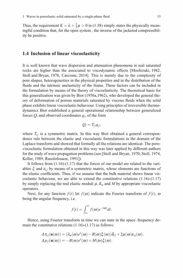
P2 waves attenuation exhibit a different behaviour than the fast P1 and shearwaves. Attenuation values are very high at low frequencies, showing that they arediffusion-type waves. After 100 Hz, all curves have a decreasing behaviour, with P2waves suffering the highest attenuation for the oil case, the lower attenuation for thegas case, and the water case having an intermediate behaviour. After 1 MHz (ultra-sonic range), P2 attenuation is negligible and P2 waves become truly propagatingwaves.

28
Fig. 1.3 Phase velocity ofP1 waves as function of fre-quency for a sample of Nivel-steiner sandstone saturated bywater, oil and gas.
0 1 2 3 4 5 6 7Frequency (Hz) - Logarithmic Scale
2500
2600
2700
2800
2900
P1 W
ave
Phas
e V
eloc
ity (
m/s
)
WaterOIlGas
Fig. 1.4 Phase velocity ofshear waves as function offrequency for a sample ofNivelsteiner sandstone satu-rated by water, oil and gas.
0 1 2 3 4 5 6 7Frequency (Hz) - Logarithmic Scale
1450
1500
1550
1600
1650
Shea
r W
ave
Phas
e V
eloc
ity (
m/s
)
WaterOilGas
Fig. 1.5 Phase velocity P2waves as function of fre-quency for a sample of Nivel-steiner sandstone saturated bywater, oil and gas.
0 1 2 3 4 5 6 7Frequency (Hz) - Logarithmic Scale
0
200
400
600
800
P2 W
ave
Phas
e V
eloc
ity (
m/s
) WaterOilGas
1.8 Application to a real sandstone

1 Waves in poroelastic solid saturated by a single-phase fluid 29
Fig. 1.6 Attenuation coeffi-cient of P1 waves as functionof frequency for a sampleof Nivelsteiner sandstonesaturated by water, oil andgas.
0 1 2 3 4 5 6 7Frequency (Hz) - Logarithmic Scale
0
0.1
0.2
0.3
0.4
P1 W
ave
Atte
nuat
ion
(dB
)
WaterOilGas
Fig. 1.7 Attenuation coef-ficient of shear waves asfunction of frequency for asample of Nivelsteiner sand-stone saturated by water, oiland gas.
0 1 2 3 4 5 6 7Frequency (Hz) - Logarithmic Scale
0
0.2
0.4
0.6
0.8
Shea
r W
ave
Atte
nuat
ion
(dB
)
WaterOilGas
1.9 Appendix 1. Models of linear viscoelasticity
First recall that for any given complex and frequency dependent modulus M(ω) thequality factor is defined by
QM(ω) =Re(M(ω))
Im(M(ω)). (1.118)
Next, we define the Zener or standard linear solid model associated with a givenelastic modulus M.
The dimensionless Zener element can be written in the form
30
Fig. 1.8 Attenuation coeffi-cient of P2 waves as functionof frequency for a sampleof Nivelsteiner sandstonesaturated by water, oil andgas.
0 1 2 3 4 5 6 7Frequency (Hz) - Logarithmic Scale
0
10
20
30
40
50
60
P2 W
ave
Atte
nuat
ion
(dB
)
WaterOilGas
Nz(ω) =1+ iωtε1+ iωtσ
. (1.119)
In (1.119) tε and tσ are relaxation times given by
tε =t0Q0
(1+√Q2
0 +1
), tσ = tε − 2 t0
Q0,
where to is a relaxation time such that 1/t0 is the center frequency of the relaxationpeak and Q0 is the minimum quality factor of the complex modulus
M(ω) =MNz(ω).
Next we formulate a model that for given elastic modulus M yields constantquality factors over a frequency range of interest.
Such behaviour is modeled by a continuous distribution of relaxation mecha-nisms based on the standard linear solid (see [Liu et al., 1976] and [Ben-Menahem and
The dimensionless complex moduli for a specific frequency can be expressed as
Nl(ω) = 1+2
πQMln
1+ iωt21+ iωt1
, (1.120)
where t1 and t2 are time constants, with t2 < t1, and the quality factor Q(ω) associ-ated with the complex modulus
M(ω) =MNl(ω) (1.121)
remains nearly constant and equal to QM over the selected frequency range. Theplex modulus in (1.121) can also be written in the equivalent form [Bourbie et al., 1987]
Sing, 1981], pp. 909).
com-
1.9 Appendix 1. Models of linear viscoelasticity

1 Waves in poroelastic solid saturated by a single-phase fluid 31
M(ω) =M
β (ω)− iγ(ω)(1.122)
where
βl(ω) = 1− 1
πQMln
1+ω2t211+ω2t22
, γl(ω) =2
πQMtan−1 ω(t1 − t2)
1+ω2t1t2. (1.123)

Chapter 2
A poroelastic solid saturated by two immisciblefluids
Abstract The derivation of Biot’s theory presented in Chapter 1 assumed a single-phase fluid. The case of a porous solid saturated by a two-phase fluid requires ageneralized argument due to the presence of capillary pressure forces. Here capil-lary forces are included in the wave propagation model using a Lagrange multiplierin the virtual complementary work principle, leading to the derivation of the con-stitutive relations. Following the ideas given in Chapter 1, the potential and kineticenergy and dissipation functions are derived to obtain the lagrangian formulation ofthe equations of motion. In particular, the dissipation function is determined consid-ering two-phase fluids and two-phase Darcy’s law. A plane wave analysis shows theexistence of three compressional waves, denoted as P1, P2 and P3, and one shearwave. A numerical example is given showing the behaviour of all waves as func-tion of saturation and frequency for a sample of Nivelsteiner sandstone saturated byeither oil-water or gas-water, water being the wetting phase.
2.1 Introduction
Theoretical formulations for the study of the deformation and elastic wave propa-gation in porous rocks with partial, multi-phase, or segregate fluid saturation havebeen presented in several papers (see [Dutta and Ode, 1979, Berryman et al., 1988,Mochizuki, 1982] among other authors).
However, none of these models incorporates the capillary forces existing whenthe pore fluids are immiscible. Consequently, the pressure variations induced bywave propagation in the different fluid phases are considered almost equal, neglect-ing possible changes in capillary pressure.
For the case of multi-phase fluids, we mention an analysis of wave propagationin porous media saturated by immiscible fluids presented in [Corapcioglu, 1996].Later, [Lo et al., 2005] derived a model for waves travelling in an elastic poroussolid permeated by two immiscible fluids incorporating both inertial and viscous
© Springer International Publishing AG 2016
in Geosystems Mathematics and Computing, DOI 10.1007/978-3-319-48457-0_2
33J.E. Santos, P.M. Gauzellino, Numerical Simulation in Applied Geophysics, Lecture Notes

34
drags in an Eulerian frame of reference, applying their model to a Columbia finesandy loam saturated by air-water and oil-water.
In this Chapter we present a general theory for this kind of problems, which at thesame time includes the effects of the ambient overburden pressure and the referencepressures of the immiscible fluids on the mechanical response of the rock.
The theoretical basis was given in [Santos et al., 1990b, Santos et al., 1990a]. Forthe study of wave propagation processes, two possible sources of energy dissipa-tion are considered in this theory: Biot-type global flow and linear viscoelasticity.The first one is included by means of a viscous dissipation density function in thelagrangian formulation and involves the relative flow velocities of the two fluidsrespect to the solid frame. The second one is incorporated by extending the elas-tic constitutive relations to the linear viscoelastic case by means of the correspon-dence principle [Biot, 1962]. In this way the real poroelastic coefficients in the con-stitutive equations are replaced by complex frequency dependent poroviscoelasticmoduli satisfying the same relations as in the elastic case. Viscoelastic behaviouris included in order to model the levels of dispersion and attenuation suffered bythe different types of waves when travelling in real rocks. A form of the frequencycorrection factors for the mass and viscous coupling coefficients in the equations ofmotion needed in the high-frequency range is also presented.
The theory is applied to determine the behaviour of all waves as function ofsaturation and frequency for a sample of Nivelsteiner sandstone saturated by eitheroil-water or gas-water.
2.2 Constitutive relations
When two immiscible fluids occupy the voids of a poroelastic solid one of them(depending on their adhesion tension), tends to preferentially wet the solid surface,spreading over it. In this way we can distinguish a wetting phase and a non-wettingone, which will be denoted with the subscripts (or superscripts) “w” and “n”, respec-tively. Let Sw and Sn denote the averaged wetting and non-wetting fluid saturations,respectively. Furthermore, let us assume that the two fluid phases completely satu-rate the porous part of the bulk material so that
Sw+Sn = 1.
The symbols Srw and Srn will denote the residual wetting and non-wetting fluidsaturations, respectively. We assume that both fluids are allowed to move inside thepore space, so that
Srn < Sn < 1−Srw
(see [Collins, 1961, Bear, 1972, Scheidegger, 1974, Peaceman, 1977]).
2.2 Constitutive relations

2 A poroelastic solid saturated by two immiscible fluids 35
At a reference initial state, we consider a volume Vb of homogeneous bulk mate-rial containing fluid volumes Vn and Vw at pressures pn and pw. In such a state wehave
V f =Vn+Vw, Sq =Vq/V f , q= n,w, φ =V f /Vb.
Also, let pn = pn +Δ pn and pw = pw +Δ pw denote the absolute pressures ofthe fluid phases, Δ pn and Δ pw representing small increments in the correspondingpressures with respect to their reference values pn and pw, and set
ΔSn = Sn−Sn =−ΔSw.
Let us, un and uw denote the averaged absolute displacement vectors of the solid,non-wetting and wetting phases, respectively. Let φ denote the effective porosityand define the relative flow vectors of the fluid phases as
uq = φ(uq−us), q= n,w. (2.1)
Also setξ q =−∇ ·uq, q= n,w.
Note that for uniform porosity Snξ n and Swξw represent the change in the cor-responding fluid contents per unit volume of bulk material [Santos et al., 1990b].Thus, if ΔVc
q denotes the part of the total change in volume ΔVq = Vq−Vq due tochanges Δ pq = pq− pq in the corresponding fluid pressures, since in equilibrium∇Sq = 0, we see that
Sqξ q =ΔVq−ΔVc
q
Vb= φ
ΔVq−ΔVcq
V f, q= n,w. (2.2)
Let Kn = C−1n and Kw = C−1
w denote the bulk moduli of the non-wetting andwetting fluids, respectively, Cn and Cw being the corresponding compressibilities.Then, by definition
ΔVcq
Vq=−Δ pq
Kq, q= n,w.
Also, neglecting second order terms,
ΔVq =V f ΔSq+SqΔVf , q= n,w,
and consequently
ξ q = φ(
ΔSqSq
+ΔVf
V f− ΔVc
q
Vq
), q= n,w.
Settingξ ∗ = Snξ n+Swξw,
it follows from (2.2) that

36
ξ ∗ = φΔVf −ΔVc
n −ΔVcw
V f.
Next, let τi j = τ i j +Δτi j, i, j = 1,2,3, be the total stress tensor of the bulk ma-terial, Δτi j being the change in the total stress with respect to a reference value τ i jcorresponding to the initial equilibrium state.
Recall that pn and pw are related through the capillary relation (see [Bear, 1972,Scheidegger, 1974, Peaceman, 1977]), which can be regarded as an equation of statefor this system:
Pca(Sn) = pn− pw = Pca(Sn)+ΔPca ≥ 0. (2.3)
Then, ignoring terms of the second order in ΔSn,
ΔPca(Sn+ΔSn) = Δ pn−Δ pw ∼= P′ca(Sn)ΔSn. (2.4)
The function Pca(Sn) is a positive and strictly increasing function of the variable Sn;hysteresis effects are ignored.
Let us consider a volume Ω of bulk material of boundary ∂Ω in static equi-librium state under the action of the surface forces f si , f
ni , f
wi , i = 1,2,3, acting on
the solid and fluid parts of ∂Ω per unit area of bulk material. These forces can bewritten in the form [Santos et al., 1990b]
f si = [τi j+φ(Snpn+Swpw)δi j]ν j, f qi =−φSqpqδi jν j, q= n,w,
where ν is the unit normal to ∂Ω .If W ∗ = W ∗(Δτi j,Δ pn,Δ pw) represents the complementary strain energy den-
sity of the system, then its complementary potential energy V ∗ is given by ([Fung, 1965,
V∗ =
∫Ω
W∗ dΩ −
∫∂Ω
( f si usi + f ni uni + f wi uwi )d(∂Ω). (2.5)
The principle of complementary virtual work for our system, including capillaryforces, can be stated in the form [Santos et al., 1990b]:
∫Ω
δW∗ dΩ =
∫∂Ω
(δ f si usi +δ f ni uni +δ f wi uwi )d(∂Ω) (2.6)
−∫
Ω[δλnw(Δ pn−Δ pw−ΔPca)+λnw(δΔ pn−δΔ pw−δΔPca)]dΩ ,
where δ denotes virtual changes and λnw is a Lagrange multiplier used to introducethe capillary relation (2.3) as a constraint. Neglecting second order terms in thedifferent increments and using (2.4) we have [Santos et al., 1990b]
δ f ni =−φ[SnδΔ pn+ pn
δΔPcaP ′
ca(Sn)
]δi jν j, (2.7)
Santos et al., 1990b])
2.2 Constitutive relations

2 A poroelastic solid saturated by two immiscible fluids 37
δ f wi =−φ[SwδΔ pw− pw
δΔPcaP ′ca(Sn)
]δi jν j, (2.8)
δ f si =−φ[SnδΔ pn+SwδΔ pw+Pca(Sn)
δΔPcaP ′ca(Sn)
]δi jν j+δΔτi jν j. (2.9)
Transforming the surface integral in (2.6) into a volume integral by meansof Gauss theorem, using equations (2.7)-(2.9), and following the argument in[Santos et al., 1990b] it can be shown that
δW∗ = εi j δΔ τi j+(Sn ξ n−λnw)δΔ pn+(Sw ξw+λnw)δΔ pw (2.10)
+(βnw ξ n+λnw)δΔPca+(ξ n−ξw)βwnw δΔPca,
where
βnw =Pca(Sn)
P ′ca(Sn)
, βwnw =
pwP ′ca(Sn)
.
Assuming that δW ∗ is an exact differential of the variables Δτi j,Δ pn,Δ pw, andΔPca, and using the capillary relation (2.3) in (2.10) we obtain
W =12
εi j Δ τi j+ξ n [(Sn +βnw+βw
nw)δΔ pn− (βnw+βwnw)Δ pw
]+ξw
[(Sw+βw
nw)Δ pw−βwnwΔ pn
=12
Δ τi jεi j +
[(Sn+βnw+βw
nw
)ξ n−βw
nwξw]Δ pn
+[(Sw+βw
nw)ξw− (βnw+βwnw)ξ n
]Δ pw
.
Set u=(us,un,uw). Assuming linear stress–strain relations W =W ∗ [Fung, 1965]and in the isotropic elastic case we obtain the following stress-strain relations:
Δτi j(u) = 2μ εi j+δi j(λues−B1ξ n−B2ξw),
ΔTn(u) =(Sn+βnw+βw
nw
)Δ pn− (βnw+βw
nw)Δ pw =−B1es+M1ξ n+M3ξw,
ΔTw(u) =(Sw+βw
nw
)Δ pw−βw
nw Δ pn =−B2es+M3ξ n+M2ξw, (2.11)
where the magnitudes Δτi j,ΔTn and ΔTw represent the generalized forces of oursystem, εi j denotes the strain tensor, and
es = εii =ΔVbVb
.
]

38
2.2.1 Relations to determine the two-phase elastic constants
Following [Gassmann, 1951], it will be assumed that μ is identical to the shear
modulus of the dry rock μm. Also, λu =Ku− 23
μ , with Ku =C−1u being the undrained
bulk modulus, computed as [Ravazzoli et al., 2003]):
Ku =Ks(Km+Ξ)
(Ks+Ξ, Ξ =
K∗f (Ks−Km)
(φ(Ks−K∗f ))
, (2.12)
K∗f = α
(γSnCn+SwCw
)−1, α = 1+(Sn+βnw)(γ −1),
γ =(
1+P′ca(Sn)SnSwCw
)(1+P
′ca(Sn)SnSwCn
)−1,
where Km = C−1m and Ks = C−1
s denote the bulk modulus of the empty matrix andthe solid grains, respectively.
In the equations above, K∗f = (C∗
f )−1 defines an effective bulk modulus for a
two–phase fluid taking into account capillary forces.Here we are assuming that the solid matrix is composed of a homogeneous ma-
terial. In the case of mixed mineralogy an effective average coefficient for Ks can beused (see [Mavko et al., 1998]).
Using the expression of Ku in (2.12), the remaining coefficients can be obtainedby using the following relations [Ravazzoli et al., 2003]:
B1 = χKu[(Sn+βnw)γ −βnw+(γ −1)βwnw],
B2 = χKu[Sw+(1− γ)βwnw],
M1 =−M3 −B1Cm(Cs−Cm)−1,
M2 = (aB2 +βwnw)b
−1,
M3 =−M2 −B2Cm(Cs−Cm)−1,
where
χ =[Cs−Cm+φ (Cm−Cu)
]α[(Cs−Cm)+φ
(Cm−Cf
)]−1,
b= φ(Cn+
1
P ′ca(Sn)SnSw
),
a= (Sn+βnw)Cs+CmCu
(Cm−Cu)
[bB2 +(Sn+βnw)
(1−CsC
−1u
)].
2.3 Inclusion of linear viscoelasticity
As indicated in Chapter 1, using the correspondence principle derived by Biot[Biot, 1956a, Biot, 1962] and assuming that the system exhibits linear viscoelastic
2.3 Inclusion of linear viscoelasticity

2 A poroelastic solid saturated by two immiscible fluids 39
behaviour, we are able to extend the constitutive relations (2.11) by simply replacingthe real elastic moduli μ ,Ku,M1,M2 and M3 by appropriate viscoelastic operators.
Using Fourier transform in time we can state this relations in the space–frequencydomain as follows:
Δτi j(u(ω)) = 2μ(ω)εi j(ω)+δi j[λu(ω)es(ω)−B1ξ n(ω)−B2ξw(ω)],(2.13)
ΔTn(u(ω)) =−B1es(ω)+M1(ω)ξ n(ω)+M3ξw(ω), (2.14)
ΔTw(u(ω)) =−B2es(ω)+M3ξ n(ω)+M2(ω)ξw(ω), (2.15)
where μ(ω),λu(ω) =Ku(ω)− 23
μ(ω),M1(ω),M2(ω) and M3(ω) are complex fre-
quency dependent poroviscoelastic moduli.Also, as indicated in Chapter 1, possible choices to make the poroviscoelastic
moduli frequency dependent are given in Appendix 1.9.
2.4 The equations of motion. Low frequency range
First we will get an expression for the complementary potential energy density V ∗d
of the system. Consider a perturbation of the system from the equilibrium state.According to (2.5)
δV∗ =∫
ΩδV
∗d dΩ =
∫∂Ω
(δ f si usi +δ f ni u
ni +δ f wi uwi )d(∂Ω).
Using equations (2.7) and (2.10), we obtain
δV∗=∫
Ω−usi δ
∂Δτi j∂x j
+uni δ∂
∂xiΔTn+uwi δ
∂∂xi
ΔTw+λ δ [ΔPca−(Δ pn−Δ pw)]dΩ .
Since we are in the linear case, the complementary strain energy W ∗ equals thestrain energy W , also V ∗
d = Vd [Fung, 1965]. Then, assuming that Vd is an exactdifferential we have
Vd =−usi∂Δτi j∂x j
+uni∂
∂xiΔTn+uwi
∂∂xi
ΔTw+λ (ΔPca− (Δ pn−Δ pw)).(2.16)
Note that thanks to (2.4) the last term in (2.16) vanishes.Thus, if u= (usi , u
ni , u
wi ) = (u j), 1 ≤ i≤ 3, 1 ≤ j ≤ 9, are chosen as generalized
coordinates and assuming that the system is conservative, from (2.16) we get
∂Vd
∂usi=−∂Δτi j
∂x j,
∂Vd
∂uni=
∂∂xi
ΔTn,∂Vd
∂uwi=
∂∂xi
ΔTw, 1 ≤ i≤ 3. (2.17)
Next, in the isotropic case the kinetic energy density Td and the dissipation densityfunction Dd have the form [Santos et al., 1990b]

40
Td =12
ρ usi usi +ρn Sn u
si u
ni +ρw Sw usi u
wi (2.18)
+12gcn u
ni u
ni +
12gcw uwi uwi +gcnw uni u
wi ,
Dd =12bcn u
ni u
ni +
12bcw uwi uwi +bcnw uni u
wi , (2.19)
where ρw and ρn are the mass densities of the wetting and the non-wetting fluidsand ρ is the density of the bulk material, i.e.,
ρ = (1−φ)ρs+Snρn+Swρw,
with ρs being the mass density of the solid grains.Also, the mass coupling coefficients gcn,g
cw and gcnw represent the inertial effects
associated with dynamic interactions among the three phases, while the coefficientsbcn,b
cw and bcnw include the viscous coupling between the solid and fluid phases. They
can be computed by the relations [Santos et al., 1990a]
gcq = SρqSq/φ , bcq = ηq(Sq)2Aq, q= n,w, (2.20)
gcnw =εS(ρnρwSnSw
) 12
φ, bcnw =
(ηnηw)12 SnSwKrnw
A, (2.21)
The factor S is known as a structure factor and is related to the tortuosity of the porespace; it can be estimated as in (1.92).
The constants ηn,ηw are the non-wetting and wetting fluid viscosities, respec-tively. Also,
A = κ(KrnKrw−K2
rnw
),
An =Krw
A, Aw =
Krn
A,
with κ , Krn, Krw and Krnw denoting the absolute and relative permeabilities, respec-tively. The relative permeabilities are assumed to be functions of the non-wettingsaturation Sn [Bear, 1972, Scheidegger, 1974, Peaceman, 1977].
The Lagrange formulation of the equations of motion is given by
ddt
(∂Td
∂ u j
)+
∂Dd
∂ u j=−∂Vd
∂u j, 1 ≤ j ≤ 9. (2.22)
In the isotropic case, from (2.17),(2.18), (2.19) and (2.22) we obtain the equations
ρ us+ρnSnun+ρwSwuw−∇ ·Δτ(u) = fs, (2.23)
ρnSnus+gcnun+gcnwu
w+bcnun+bcnwu
w+∇ΔFn(u) = fn, (2.24)
ρwSwus+gcnwun+gcwu
w+bcnwun+bcwu
w+∇ΔFw(u) = fw, (2.25)
2.4 The equations of motion. Low frequency range

2 A poroelastic solid saturated by two immiscible fluids 41
where fs, fn and fw indicate external forces in the solid, non-wetting and wettingphases, respectively.
To obtain (2.23)-(2.25) we have applied the dimensional argument given in[Santos et al., 1990b] using that Sn can be assumed independent of time.
2.5 The equations of motion. High frequency range
As explained in Chapter 1 for the case of single–phase fluids, in the high–frequencyrange the viscous and mass coupling coefficients become frequency dependent. Thiseffect is associated with the departure of the flow from the laminar Poiseuille type atthe pore scale, which occurs for frequencies greater than some characteristic value.Since we have two immiscible fluids flowing within the pore space and three relativepermeability functions, following the ideas in [Berryman et al., 1988], we define forthis model three characteristic frequencies of the form
ωqc =
SqηqφAq
(Sρq), q= n,w, (2.26)
ωnwc =
φ (ηnηw)12(SnSw) 1
2 Krnw
(εA S(ρnρw)12 )
. (2.27)
These frequencies are obtained by equating the inertial and viscous drag terms as-sociated with each fluid phase and using (2.20) and (2.21). For frequencies biggerthan the minimum of the three characteristic frequencies defined above, the massand viscous coupling coefficients are defined as follows.
If we employ the frequency correction function F(ω) = FR(ω)+FI(ω) definedin Chapter 1, equation (1.93), then we define
gq(ω) = gcq+ηq(Sq)2AqFI(θq(ω))
ω, q= n,w,
gnw(ω) = gcnw+(ηnηw)
12 SnSwKrnwFI(θnw)(ωA )
,
bq(ω) = bcq FR(θq), q= n,w,nw.
The arguments θq(ω) are defined as follows [Santos et al., 2005a]
θq(ω) = aqp
√ω ρ j/ηq, aqp = 2
√KkrqA0/φ , q= n,w,nw,
where A0 denotes the Kozeny-Carman constant.If instead the we employ the frequency correction function in (1.94) in Chapter
1 then we define

42
gq(ω) = gcq+ηqa
qpF
qI (ω)
ω, bq(ω) = bcqF
qR (ω), q= n,w,
gnw(ω) = gcnw+(ηnηw)
1/2bcnwFnwI (ω)
ω, bnw(ω) = bcnwF
nwR (ω),
where gcq,bcq,g
cnw and bcnw are defined in (2.20)-(2.21) and
Fq(ω) =
(1− 4iS2κKrq
xqΛ 2q φ
), xq =
ηqφSqωκKrqρq
, Λ 2q =
8SκKrq
φSq, q= n,w,
Fnw(ω) =
(1− 4iS2 κ Krnw
xnwΛ 2nw φ
), xnw =
(ηnηw)1/2 φ (SnSw)1/2
ω κ Krnw (ρnρw)1/2,
Λ 2nw =
8Sκ Krnw
φ (SnSw)1/2.
Next, from (2.13)-(2.15) and (2.23)-(2.25) we can state the equations of motion inthe space-frequency domain (including viscoelasticity effects if needed) as follows
−ω2 (ρ us(ω)+ρn Snun(ω)+ρw Swuw(ω))−∇ ·Δτ(u(ω)) = fs(ω),(2.28)
−ω2 (ρn Snus(ω)+gnun(ω)+gnwuw(ω))
(2.29)
+iω bnun(ω)+ iω bnwuw(ω)+∇ΔTn(u(ω)) = fn(ω),
−ω2 (ρw Swus(ω)+gnwun(ω)+gwuw(ω))+ iω bwuw (2.30)
+iω bnwun(ω)+∇ΔTw(u(ω)) = fw(ω).
For a spatially homogeneous medium and in the absence of body forces, theequations of motion (2.28)-(2.30) take the form:
−ω2 (ρus(ω)+ρn Snun(ω) +ρw Swuw(ω))= Eu∇∇ ·us(ω)
−μ ∇×∇×us(ω) +B1∇(∇ ·un(ω))+B2∇(∇ ·uw(ω)), (2.31)
−ω2 (ρn Snus(ω)+gn(ω)un(ω)+gnw(ω)uw(ω))
+iωbn(ω)un(ω)+ iωbnw(ω)uw(ω)
= B1∇(∇ ·us)+M1(ω)∇(∇ ·un(ω)) +M3∇(∇ ·uw(ω)), (2.32)
−ω2 (ρw Sw us(ω)+gnw(ω)un(ω)+gw(ω)uw(ω)
)+iωbw(ω)uw(ω)+ iωbnw(ω)un(ω)
= B2∇(∇ ·us(ω))+M3∇(∇ ·un)(ω)+M2(ω)∇(∇ ·uw(ω)), (2.33)
where
Eu = Ku+43
μ .
2.5 The equations of motion. High frequency range

2 A poroelastic solid saturated by two immiscible fluids 43
Taking into account the fact that FR(θ) → 1 and FI(θ)/ω → 0 as ω → 0 we mayregard (2.31)-(2.33) as the general form of the equations of motion for frequenciesranging from the seismic to the ultrasonic range.
2.6 Plane wave analysis
Taking the divergence in (2.31)-(2.33) we get
−ω2ρes−ω2ρoSnen−ω2ρwSwe
w (2.34)
= Eu∇2es+B1∇2en+B2∇2ew,
−ω2ρnSnes−ω2gn e
n−ω2gnw uw+ iωbne
n+ iωbnwew (2.35)
= B1Δ es+M1∇2en+M3∇2ew,
−ω2ρwSwes−ω2gnw e
n−ω2gw ew+ iωbnwe
n+ iωbwew (2.36)
= B2∇2 es+M3∇2en+M2∇2ew.
Replacing in (2.34)-(2.36) a plane compressional wave of angular frequency ω andwave number = r+ ii travelling in the x1–direction of the form
es =C()s ei(x1−ωt) =C()
s e−ix1eir(x1− ωrt),
en =C()n ei(x1−ωt) =C()
n e−ix1eir(x1− ωrt),
ew =C()w ei(x1−ωt) =C()
w e−ix1eir(x1− ωrt),
and setting
γ =ω
leads to the eigenvalue problem
γ2AC(γ) = EC(γ),
where
A =
⎛⎝ ρ ρn ρw
ρn gn gnwρw gnw gw
⎞⎠ , E =
⎛⎝Eu B1 B2
B1 M1 M3
B2 M3 M2
⎞⎠ , C γ =
⎛⎝C γs
C γn
C γw
⎞⎠ ,
and
gn = gn+ ibnω, gw = gw+ i
bwω
, gnw = gn+ ibnwω
.
Hence, to determine the complex wave-numbers = r+ ii it is sufficient to solvethe problem

44
det(S − γ2I) = 0,
where
S = A−1
E .
The three physically meaningful solutions (i.e., i > 0) (γ( j))2, j = 1,2,3 determine
three phase velocities v( j) and attenuation coefficients b( j)i corresponding to the P1and P2 and P3 compressional modes of propagation.
The P1 is the analogue of the classical fast P-wave propagating in elastic or vis-coelastic isotropic solids and is associated with the motion of both solid and fluidsmoving in phase.
The P2 and P3 waves are slow waves strongly attenuated in the low frequencyrange; the motion of these slow waves will be analyzed numerically in Subsection2.7.1.
The numerical evidence of the existence of a second compressional slow wavewas shown in [Santos et al., 2004b].
For rotational waves, consider a plane rotational wave of angular frequency ωand wave number = r+ ii travelling in the x1–direction:
ks =C()1 e−ix1eir(x1− ω
rt), (2.37)
kn =C()2 e−ix1eir(x1− ω
rt), (2.38)
kw =C()3 e−ix1eir(x1− ω
rt). (2.39)
Then take the curl operator in (2.31)-(2.33) and substitute (2.37)-(2.39) in the re-sulting equations to obtain
that allows to compute the phase velocity v(s) and attenuation coefficients b(s) forthe shear mode.
The phase velocities and attenuation coefficients for all waves are given by
v( j) =ω
|( j)r |, b( j) = (2π) ·8.685889(|(s)i |/|(s)r |), j = 1,2,3,s.
2.7 Application to a real sandstone
In this section we compute phase velocities and attenuation coefficients for a sampleof Nivelsteiner sandstone. The material properties of the sandstone and the saturant
2.7 Application to a real sandstone
γ2 = µ
(ρ− ρnSn
(gwρwSn − gnwρwSw
)+ ρwSw
(gnρwSw − gnwρnSn
)gngw − (gnw)2
)−1

2 A poroelastic solid saturated by two immiscible fluids 45
fluids, water, oil and gas, are given in Table 1.1. Water is considered the wettingphase.
The relative permeability functions Krn(Sn) and Krw(Sn) and the capillary pres-sure Pca(Sn) used in the following examples are computed using the relations[Douglas Jr. et al., 1993, Ravazzoli et al., 2003]:
Krn(Sn) =
(1− 1−Sn
1−Srn
)2
, krw(Sn) =
(1−Sn−Srw
1−Srw
)2
, (2.40)
Pca(Sn) = A
(1
(Sn+Srw−1)2 − S2rn
S2n(1−Srn−Srw)2
). (2.41)
Also, we takeKrnw(Sn) =
√ε Krn(Sn)Krw(Sn), (2.42)
with the capillary pressure amplitude coefficient A equals 3 kPa and ε = 0.01. Theresidual saturation values are Srn = Srw = 0.002.
The relations (2.40)-(2.42) are based on laboratory experiments performed ondifferent porous rocks during imbibition and drainage processes (neglecting hys-teresis effects). However, it must be pointed out that those functions depend on thenature of the porous medium and the wettability of the pore fluids involved.
2.7.1 Characterization of the compressional modes of propagation
To study how the solid and fluid phases move in the three compressional modes,following [Biot, 1956a] it is convenient to write the equations of motion for theelastic case (zero viscosity) in terms of the solid displacement us and the absolutefluid displacements un and uw. Set
en = ∇ · un, ew = ∇ · uw.
Using (2.1) in (2.31)-(2.33), taking divergence in the resulting equations and replac-ing a plane compressional wave of angular frequency ω and (real) wave number travelling in the x1–direction of the form
es = C()s ei(x1−ω
t), en = C()n ei(x1−ω
t), ew = C()w ei(x1−ω
t),
leads to the eigenvalue problem
γ2A C() = E C(γ),
where
γ =ω, C γ =
(C γs ,C
γn ,C
γw
)t,

46
A =
⎛⎝ρ −φ(ρnSn+ρwSw) φρnSn φρwSwρnSn−φ(gn+gnw) φgn φgnwρwSw−φ(gw+gnw) φgnw φgw
⎞⎠, E =
⎛⎝ Eu−φ(B1 +B2) φB1 φB2
B1 −φ(M1 +M3) φM1 φM3
B2 −φ(M2 +M3) φM3 φM2
⎞⎠.In (2.43) we illustrate symbolically in the matrices referred to as C1 and C2 the
two possibly cases in which the three phases can move.Column j in matrices C1 and C2 shows the signs of the components of the eigen-
vectors associated with the phase velocities v( j), j = 1,2,3 ordered in decreasingorder. The symbols s,n,w in the first column of these matrices indicate the solid,non-wetting and wetting phases components of each column eigenvector.
These results were obtained numerically for random values of saturations of thewetting and non-wetting fluids and reference wetting pressure pw.
The numerical results allow us to conclude that
• P1 waves: the solid moves in phase with the wetting and non-wetting fluid phases.This is the fast compressional P1 wave in the classic Biot theory (column 1 inmatrices C1 and C2).
• P2 waves: the two fluids move in phase and in opposite phase with the solid. Thisis the analogue of the slow Biot wave for single-phase fluids (column 2 in matrixC1 and column 3 in matrix C2).
• P3 waves: the solid moves in phase with the non-wetting phase and in oppositephase with the wetting phase, and the two fluid phases move in opposite phase(column 3 in matrix C1 and column 2 in matrix C2). This is a new mode notpresent in the case of single-phase fluids ( see [Santos et al., 2004b]).
This analysis also shows that depending on the value of the reference pressurepw and the saturation values of the non-wetting and wetting phases the P3 wave hasa faster velocity than the P2 wave.
C1 =
⎡⎢⎢⎣v(1) v(2) v(3)
s + − +n + + +w + + −
⎤⎥⎥⎦ , C2 =
⎡⎢⎢⎣v(1) v(2) v(3)
s + + −n + + +w + − +
⎤⎥⎥⎦ . (2.43)
2.7.2 Analysis of all waves in the purely elastic case
Let us analyze the behaviour of all waves in the elastic case (zero viscosity) as func-tion of saturation of the non-wetting phase. The behaviour of P1 waves is shown inFigure 2.1. The Figure shows the characteristic decreasing behaviour for oil-watermixtures shown by the corresponding Gassmann velocity vpG defined in (2.44). Forgas-water mixtures, at very low gas saturation we see a sharp decreasing of veloc-ities until a low gas saturation value at which a continuous increasing behaviour isobserved.
2.7 Application to a real sandstone

Fig. 2.1 Phase velocity ofP1 waves as function of non-wetting phase saturation.
0 0.2 0.4 0.6 0.8Nonwetting Phase Saturation
2500
2600
2700
2800
P1 W
ave
Phas
e V
eloc
ity (
m/s
) Gas-waterOil-water
Figure 2.2 exhibits strong differences in P2 phase velocities for the gas-waterand oil-water mixtures, and in both cases show decreasing velocities as non-wettingsaturation increases. Besides, P2 waves for the gas-water mixture have slower ve-locities than the oil-water mixture because the opposite motion of the fluid and solidphases should be smaller for lower density fluids.
Fig. 2.2 Phase velocity ofP2 waves as function of non-wetting phase saturation.
0 0.2 0.4 0.6 0.8Nonwetting Phase Saturation
0
200
400
600
800
P2 W
ave
Phas
e V
eloc
ity (
m/s
)
Gas-waterOil-water
2 A poroelastic solid saturated by two immiscible fluids 47

48
Figure 2.3 shows that P3 waves phase velocities for gas-water mixtures are al-most independent of gas saturation, while for oil-water mixtures they decrease asoil saturation increases. The P3 wave is associated with the existence of capillaryforces, and it is due to the in-phase motion of the solid and non-wetting phases,what explains its higher values for oil-water mixtures as compared with gas-watermixtures.
Fig. 2.3 Phase velocity ofP3 waves as function of non-wetting phase saturation.
0 0.2 0.4 0.6 0.8Nonwetting Phase Saturation
0
10
20
30
40
50P3
Wav
e Ph
ase
velo
city
(m
/s)
Gas-waterOil-water
The behaviour of shear waves as function of non-wetting phase saturation isshown in Figure 2.4. For both mixtures, shear velocities exhibit increasing valuesas non-wetting saturation increases. The higher values of phase velocities for gas-water mixtures are explained by the fact that, for a fixed non-wetting phase satura-tion value, the fluid bulk density is smaller for the gas-water than for the oil-watermixture.
2.7.3 Analysis of all waves as function of frequency in the generaldissipative case
Let us analyze next the behaviour of all waves for the general case in which dissipa-tion due to the relative motion of the viscous fluids and the solid phase is considered.Besides, high frequency corrections of the viscodynamic coefficients are made forfrequencies above the minimum of the critical frequencies defined in (2.26)-(2.27).
Figures 2.5, 2.6, 2.7 and 2.8 show phase velocities for P1, shear, P2 and P3 wavesas function of frequency, respectively, while 2.9, 2.10, 2.11 and 2.12 display the cor-responding attenuation coefficients. The non-wetting fluids are gas and oil of satu-
2.7 Application to a real sandstone

Fig. 2.4 Phase velocity ofshear waves as function ofnon-wetting phase saturation.
0 0.2 0.4 0.6 0.8Nonwetting Phase Saturation
1500
1520
1540
1560
1580
1600
Shea
r W
ave
Pha
se V
eloc
ity (
m/s
) Gas-waterOil-water
rations Sn = 0.1,n= g,o or Sn = 0.5,n= g,o. For P1 and shear waves in Figures 2.5and 2.6 very little dispersion is observed in the whole range of frequencies. At highfrequencies velocities stabilize at constant vales, and at zero frequency velocitiestend to the Gassmann velocities
vpG =
√Ku+
43
μ, vsG =
√μρ. (2.44)
At fixed water saturation Sw = 0.9, P1 waves in Figure 2.5 show higher velocitiesfor oil-water than for gas-water mixtures, while shear waves in this case, Figure2.6, exhibit very little differences in velocities. On the other hand, at fixed water
for gas-water mixtures, but for shear waves in this case the opposite behaviour isobserved, due to the lower density of gas and that the shear modulus is independentof the saturant fluids.
Phase velocities of P2 and P3 waves have a quite different behaviour than the fastP1 and shear waves. These waves suffer noticeable dispersion on the whole rangeof frequencies and velocities tend to zero at low frequencies. At ultrasonic frequen-cies, the inertial terms are dominant and velocities stabilize at constant values. Forthe highest saturation of the wetting phase (Sw = 0.9) P2 waves have the highest ve-locities for the non-wetting fluid of higher viscosity (oil), while P3 waves show theopposite behaviour. For equal proportions of wetting and non-wetting fluids, the P2and P3 waves exhibit higher velocities when the non-wetting fluid is that of higherviscosity (oil).
Figures 2.9 and 2.10 show that attenuation for P1 and shear waves is negligibleat low frequencies. Also, for P1 waves and equal proportions of wetting and non-wetting fluids, attenuation is higher for the fluid of lower viscosity (gas). For watersaturation Sw = 0.9 attenuation is higher when gas is the non-wetting phase; this isthe case exhibiting the highest attenuation.
2 A poroelastic solid saturated by two immiscible fluids 49
saturation Sw = 0.5, again P1 waves have higher velocities for oil-water than

50
For shear waves and water saturation Sw = 0.9, Figure 2.10 shows that attenua-tion is dependent of the non-wetting phase, with one attenuation peak for gas-watermixtures and two peaks for oil-water mixtures, one lower than the gas-water peakand the second at an ultrasonic frequency of about 1 MHz. For equal proportionsof wetting and non-wetting fluids, the attenuation peak moves to higher frequenciesfor the fluid of higher viscosity (oil).
In Figures 2.11 and 2.12 can be observed that attenuation for P2 and P3 waves isvery high at low frequencies up to about 100 Hz, indicating the diffusive characterof these two modes in the seismic range. Above 100 Hz, attenuation decays to zeroat ultrasonic frequencies, where the P2 and P3 waves become propagating modes.
For P2 waves and water saturation Sw = 0.9, attenuation is independent of thenon-wetting fluids, and for equal proportions of wetting and non-wetting fluids, theoil phase is the one suffering the highest attenuation of all cases.
For P3 waves and equal proportions of wetting and non-wetting fluids attenuationis higher when oil is the non-wetting phase, and for water saturation Sw = 0.9 thehighest attenuation is seen when oil is the non-wetting phase; this case is the oneexhibiting the highest attenuation.
Fig. 2.5 Phase velocity ofP1 waves as function offrequency for two differentvalues of oil and gas satura-tions.
-1 0 1 2 3 4 5 6 7Frequency (Hz) - Logarithmic Scale
2400
2500
2600
2700
2800
P1 W
ave
Phas
e V
eloc
ity (
m/s
) Sg = 0.1, Sw = 0.9So = 0.1, Sw = 0.9Sg = 0.5, Sw = 0.5So = 0.5, Sw = 0.5
2.7 Application to a real sandstone

0 2 4 6Frequency (Hz) - Logaritmic Scale
1450
1500
1550
1600
Shea
r W
ave
Phas
e V
eloc
ity (
m/s
)
Sg = 0.1, Sw = 0.9So = 0.1, Sw = 0.9Sg = 0.5, Sw = 0.5So = 0.5, Sw = 0.5
-1 0 1 2 3 4 5 6 7Frequency (Hz) - Logarithmic Scale
0
100
200
300
400
500
600
700
P2 W
ave
Phas
e V
eloc
ity (
m/s
) Sg = 0.1, Sw = 0.9So = 0.1, Sw = 0.9Sg = 0.5, Sw = 0.5So = 0.5, Sw = 0.5
-1 0 1 2 3 4 5 6 7Frequency (Hz) - Logarithmic Scale
0
50
100
150
200
P3 W
ave
Phas
e V
eloc
ity (
m/s
)
Sg = 0.1, Sw = 0.9So = 0.1, Sw = 0.9Sg = 0.5, Sw = 0.5So = 0.5, Sw = 0.5
2 A poroelastic solid saturated by two immiscible fluids 51
Fig. 2.6 Phase velocity ofshear waves as function offrequency for two differentvalues of oil and gas satura-tions.
Fig. 2.7 Phase velocity ofP2 waves as function offrequency for two differentvalues of oil and gas satura-tions.
Fig. 2.8 Phase velocity ofP3 waves as function offrequency for two differentvalues of oil and gas satura-tions.

52
-1 0 1 2 3 4 5 6 7Frequency (Hz) - Logarithmic Scale
0
0.1
0.2
0.3
0.4
0.5
P1 W
ave
Atte
nuat
ion
(dB
)
Sg = 0.1, Sw = 0.9So = 0.1, Sw = 0.9Sg = 0.5, Sw = 0.5So = 0.5, Sw = 0.5
0 2 4 6Frequency (Hz) - Logarithmic Scale
0
0.2
0.4
0.6
0.8
Shea
r W
ave
Atte
nuat
ion
(dB
)
Sg=0.1, Sw=0.9So=0.1, Sw=0.9Sg=0.5, Sw=0.5So=0.5, Sw=0.5
-1 0 1 2 3 4 5 6 7Frequency (Hz) - Logarithmic Scale
0
10
20
30
40
50
60
P3 W
ave
Atte
nuat
ion
(dB
)
Sg = 0.1, Sw = 0.9So = 0.1, Sw = 0.9Sg = 0.5, Sw = 0.5So = 0.5, Sw = 0.5
2.7 Application to a real sandstone
Fig. 2.9 Attenuation coeffi-cient of P1 waves as functionof frequency for two dif-ferent values of oil and gassaturations.
Fig. 2.10 Attenuation co-efficient of shear waves asfunction of frequency for twodifferent values of oil and gassaturations.
Fig. 2.11 Attenuation coeffi-cient of P2 waves as functionof frequency for two dif-ferent values of oil and gassaturations.
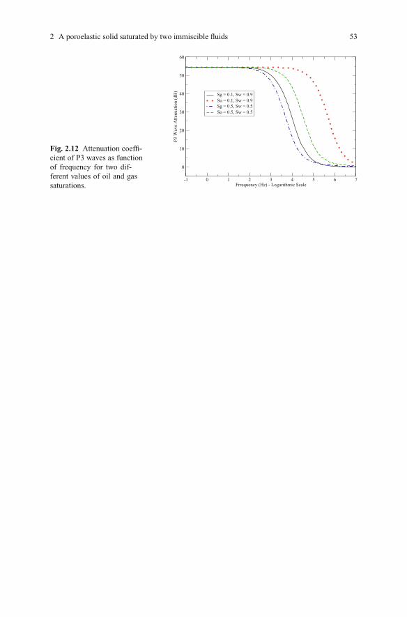
Fig. 2.12 Attenuation coeffi-cient of P3 waves as functionof frequency for two dif-ferent values of oil and gassaturations.
-1 0 1 2 3 4 5 6 7Frrequency (Hz) - Logarithmic Scale
0
10
20
30
40
50
60
P3 W
ave
Atte
nuat
ion
(dB
)
Sg = 0.1, Sw = 0.9So = 0.1, Sw = 0.9Sg = 0.5, Sw = 0.5So = 0.5, Sw = 0.5
2 A poroelastic solid saturated by two immiscible fluids 53

Chapter 3
A poroelastic solid saturated by a three-phasefluid
Abstract A theory to describe the propagation of waves in a poroelastic solid satu-rated by a three-phase fluid is presented and anlyzed. The model takes into accountthe existence of two capillary and three relative permeability functions, assumed todepend on the non-wetting fluid saturations. A plane wave analysis predicts the ex-istence of four compressional waves, denoted as P1, P2, P3 and P4, and one shearwave, all of them suffering attenuation and dispersion effects. A numerical exam-ple showing the behaviour of all waves as function of saturation and frequency in asample of Nivelsteiner sandstone saturated by water, oil and gas is presented.
3.1 Introduction
This Chapter presents a model to describe the propagation of waves in a poroelasticsolid saturated by three immiscible, compressible, viscous fluids, assumed to bewater, oil and gas.
Capillary pressure effects due to pressure differences between the oil and wa-ter and the oil and gas phases are included in the model by introducing Lagrangemultipliers in the principle of virtual complementary work [Fung, 1965]. Capillarypressures and relative permeability are assumed to be functions of saturation of thenon-wetting phases.
First we determine the strain energy density in terms of the generalized forcesand strains of the system, leading us to obtain the constitutive relations. Then thekinetic energy and dissipation density functions are computed allowing to define theLagrange equations of motion.
A plane wave analysis, shows the existence of four compressional waves, denotedas P1, P2, P3 and P4 waves and one shear wave. The model is applied to compute thephase velocities and attenuation coefficients for a sample of Nivelsteiner sandstonesaturated by water, oil and gas, with water assumed to be the wetting phase.
© Springer International Publishing AG 2016
in Geosystems Mathematics and Computing, DOI 10.1007/978-3-319-48457-0_3
55J.E. Santos, P.M. Gauzellino, Numerical Simulation in Applied Geophysics, Lecture Notes
56
3.2 Constitutive relations
Consider a porous solid Ω saturated by a three-phase fluid, taken to be oil, waterand gas in, and referred to by the indices or super-indices o,w,g, respectively. LetSθ = Sθ (x) denote the saturation of the θ -fluid phase. We assume that the threephases completely saturate the porous part of Ω , denoted by Ωp, and that all fluidphases are allowed to move within the pore space. Hence, with Sro, Srw and Srgdenoting the residual oil, water and gas saturations, respectively, we assume that
Sg+So+Sw = 1, Srθ < Sθ < 1−Srl −Srm, θ = o,w,g, l,m = θ .
Let φ = φ(x) be the effective porosity in Ω and let us,T , uθ ,T ,θ = o,w,g, denote thelocally averaged solid and absolute θ -fluid displacements in Ω .
Consider an initial state of equilibrium about displacements us, uθ
and let usdefine the infinitesimal displacements
us = us,T −us, uθ = uθ ,T − uθ, θ = o,w,g.
Let τi j = τ i j+Δ τi j and σi j = σ i j+Δ σi j be the total stress tensor in the bulk ma-terial and the stress tensor in the solid part of Ω , respectively, where Δ τi j and Δ σi j
represent changes in the corresponding stresses with respect to reference stresses τ i jand σ i j associated with the initial equilibrium state.
Let pθ = pθ +Δ pθ , θ = o,w,g be the θ -fluid pressure, with Δ pθ being the in-crement with respect to given reference pressures pθ in the initial equilibrium state.Also set
σθ =−φ Sθ pθ , θ = g,o,w, σ f = σo+σw+σg.
τi j = σi j+δi j σ f .
Next, following the ideas given in Chapter 2 for the case of two-phase fluids,we proceed to derive the strain-stress relations for our system using the principle ofvirtual complementary work [Fung, 1965] .
Let us consider a domain Ω of bulk material with boundary ∂Ω , assumed to be
initially in static equilibrium under the action of surface forces fθi , θ = s,g,o,w,
where fθi represents the force in the θ−part of ∂Ω per unit of surface area of bulk
material. Thus,
fsi = σ i j ν j, f
θi =−φ Sθ pθ δi j ν j, θ = o,w,g,
where Sθ denotes the θ -fluid saturation in the initial equilibrium state. Now, con-
sider a new system of surface forces f θi superimposed on the original system f
θi
such that Ω remains in equilibrium under the action of the total surface forces
3.2 Constitutive relations
Then, with δi j denoting the Kronecker delta,

3 A poroelastic solid saturated by a three-phase fluid 57
f θ ,Ti = f
θi + f θ
i , θ = s,o,w,g.
Since the fluids are at rest, all fluid pressures are constant on Ω and the total stressfield is in equilibrium. Hence,
∇pθ =∂ pθ∂xi
= 0, θ = o,w,g, ∇ · τ =∂τi j∂x j
= 0. (3.1)
In a poroelastic medium saturated by a three-phase fluid, we have two independentcapillary pressure functions Pcow and Pcgo. In the most general case, they depend ontwo fluid saturations and the spatial position. Following [Chavent and Jaffre, 1986],here we suppress the explicit spatial dependence of the capillary pressure functionsand assume that they depend only on one of the fluid saturations as follows: For(l,m) = (o,w),(g,o),
Pclm = Pclm(Sl) = (pl +Δ pl)− (pm+Δ pm) = Pclm(Sl)+Δ pl −Δ pm ≥ 0,(3.2)
with the functions Pcow(So) and Pcgo(Sg) being strictly increasing functions of Soand Sg, respectively. Set
ΔPclm = ΔPclm(Sl) = Δ pl −Δ pm, (l,m) = (o,w),(g,o),
ΔSθ = Sθ −Sθ , θ = o,w,g.
Neglecting terms of the second order in ΔSg and ΔSo we have that
ΔPclm = Pc′lm(Sl)ΔSl , (l,m) = (o,w),(g,o).
Next, note that it follows from (3.1) and (3.2) that in the initial equilibrium state(at which Δ pg = Δ po = Δ pw = 0),
Pc′go(Sg)∇Sg = ∇pg−∇po = 0, Pc′ow(So)∇So = ∇po−∇pw = 0.
Since it is the case that Pc′go > 0 and Pc′ow > 0, we see that
∇Sg = 0, ∇So = 0.
Let W ∗=W ∗(Δτi j, Δ po, Δ pw, Δ pg, ΔPcgo,ΔPcow) be the complementary strainenergy density. Introducing two Lagrange multipliers λow,λgo to include the capil-lary relations (3.2) as constrains, the complementary virtual work principle for oursystem [Fung, 1965] can be stated as∫
ΩδW
∗ dΩ =
∫∂Ω
(δ f si usi +δ f oi uoi +δ f wi uwi +δ f gi ugi )d(∂Ω) (3.3)
+∫
Ω[δλow(Δ po−Δ pw−ΔPcow)+λow(δΔ po−δΔ pw−δΔPcow)]dΩ
+∫
Ω[δλgo(Δ pg−Δ po−ΔPcgo)+λgo(δΔ pg−δΔ po−δΔPcgo)]dΩ ,

58
where δ f θi ,θ =s,o,w,g are the virtual forces and δΔτ i j,δΔ po,δΔ pw,δΔ pg,δΔPcow
and δΔPcgo are the virtual stresses.Next, let
uθ = φ(uθ −us), ξ θ =−∇ ·uθ , θ = o,w,g, u= (us,uo,uw,ug). (3.4)
For uniform porosity, Sθ ξ θ measures the amount of the θ -fluid entering or leavinga unit cube of bulk material.
Next, computing the virtual forces δ f θi ,θ = s,o,w,g in terms of the virtual
stresses and using that Ω remains in equilibrium, from (3.3) we conclude that∫Ω
δW ∗ dx=∫
Ω
[εi j δ Δτi j+(So ξ o−λow+λgo)δ Δ po+(Sw ξw+λow)δ Δ pw
+(Sg ξ g−λgo)δ Δ pg+(βow ξ o+βwow (ξ o−ξw) +λow)δ ΔPcow (3.5)
+((βgo+β owgo )ξ g+βw
go (ξ g−ξw)+λgo)δ ΔPcgo+(Δ po−Δ pw−ΔPcow)δ λow+(Δ pg−Δ po−ΔPcgo)δ λgo] dΩ
where
βow =Pcow(So)
Pc′ow(So), βw
ow =pw
Pc′ow(So),
βgo =Pcgo(Sg)
Pc′go(Sg), β ow
go =Pcow(So)
Pc′go(Sg), βw
go =pw
Pc′go(So).
SinceδW∗must be an exact differential in the stresses(Δτ ij,Δpo,Δpw,Δpg,ΔPcow,ΔPcgo),it follows from (3.5) that (see [Santos and Savioli, 2015, Santos and Savioli, 2016])
δW∗ = εi j δ Δ τi j+(So ξ o−λow+λgo)δΔ po+(Sw ξw+λow)δ Δ pw
+(Sg ξ g−λgo)δΔ pg+(βow ξ o+βwow(ξ o−ξw)+λow)δ ΔPcow
+(βgo+β owgo )ξ g+βw
go(ξ g−ξw)+λgo)ΔPcgo. (3.6)
In the linear isotropic case W ∗ is a quadratic positive-definite form in the linearand quadratic invariants of Δτi j and the scalars Δ po, Δ pw, Δ pg, ΔPcow, ΔPcgo.
Thus, using that ΔPcow = Δ po−Δ pw and ΔPcgo = Δ pg−Δ po to eliminate theLagrange multipliers, from (3.6) the following strain-stress relations are obtained:
εi j =1
2 μΔτi j+δi j(DΔτ −F1 Δ po−F2 Δ pw−F3 Δ pg), (3.7)
To ≡ (So+βow+βw
ow)ξ o+(βwgo−βw
ow)ξw− (βgo+β owgo +βw
go)ξ g (3.8)
=−F1Δτ +H1 Δ po+H4 Δ pw+H5 Δ pg,
Tw ≡ (Sw+βw
ow)ξw− (βow+βwow)ξ o (3.9)
=−F2Δτ +H4 Δ po+H2 Δ pw+H6 Δ pg,
Tg ≡ (Sg+βgo+β ow
go +βwgo)ξ g−βw
goξw (3.10)
3.2 Constitutive relations
3 A poroelastic solid saturated by a three-phase fluid 59
=−F3Δτ +H5 Δ po+H6 Δ pw+H3Δ pg.
Also, eliminating the Lagrange multipliers in (3.6) and using that in the linearcase W = W ∗ [Fung, 1965] we see that
W =12(εi j Δ τi j+T
oΔ po+TwΔ pw+T
gΔ pg) (3.11)
=12(Δ τi j εi j+ΔF
oξ o+ΔFwξw+ΔF
gξ g) ,
where
ΔFo ≡ (So+βow+βw
ow)Δ po− (βow+βwow)Δ pw,
ΔFw ≡ (Sw+βw
ow)Δ pw+(βwgo−βw
ow)Δ po−βwgoΔ pg,
ΔFg ≡ (Sg+βgo+β ow
go +βwgo)Δ pg− (βgo+β ow
go +βwgo)Δ po.
The variables εi j,T θ ,θ = o,w,g, in (3.7-(3.10) are the generalized strains of oursystem, while Δτi j and ΔF θ ,θ = o,w,g, multiplying the strains εi j and the changesin fluid content ξ θ ,θ = o,w,g in (3.11), are the generalized forces of our system.
Inverting the strain-stress relations (3.7)-(3.10) the following stress-strain rela-tions are derived:
Δτi j(u) = 2μ εi j+δi j(λues−B1 ξ o−B2 ξw−B3ξ g), (3.12)
ΔFo(u) =−B1 e
s+M1 ξ o+M4 ξw+M5 ξ g, (3.13)
ΔFw(u) =−B2 e
s+M4 ξ o+M2 ξw+M6 ξ g, (3.14)
ΔFg(u) =−B3 e
s+M5 ξ o+M6 ξw+M3 ξ g. (3.15)
Expressions to determine the elastic constants in (3.12)-(3.15) in terms of theproperties of the individual solid and fluid phases are given in Appendix 3.6.
3.3 The equations of motion. Low frequency range
Next, consider a perturbation of system from the equilibrium state. The potentialenergy V is
V =
∫Ω
Vd dΩ =∫
ΩW dΩ −
∫∂Ω
( f si usi + f oi u
oi + f wi uwi + f gi u
gi )d(∂Ω),(3.16)
where V and Vd denote the complementary energy and its density, respectively.Since W = W ∗, also V = V ∗. Then transform the surface integral in (3.16) into avolume integral and use the argument leading to (3.5) to see that
δVd =−usi∂
∂x jΔτi j+ ∑
θ=o,w,g
uθi
∂∂xi
ΔFθ .

60
Choosing usi ,uoi ,u
wi ,u
gi as generalized coordinates and assuming that the system is
conservative we obtain the relations
∂Vd
∂usi=− ∂
∂x jΔτi j,
∂Vd
∂uθi
=∂
∂xiΔF
θ , θ = o,w,g.
Let ρθ , θ = s,o,w,g, be the mass densities of the θ -phase and let
ρ = (1−φ)ρs+φ( ∑θ=o,w,g
ρθSθ )
denote the bulk density.Let Krθ (Sθ ),θ = o,w,g, denote the three-phase relative permeability functions
[Peaceman, 1977], and let gθ , bθ , θ = o,w,g, and glt , blt , (l, t)= (o,w),(o,g),(w,g),denote the mass and viscous coupling coefficients.
In the low frequency range,these coefficients are defined by the relations
gcθ = Sθ ρθS/φ , (3.17)
bcθ =S
2θ ηθ
κKrθ, θ = o,w,g, (3.18)
gclt = ε
(S
√Sl St
√ρl ρt
φ
), (3.19)
blt = ε(Sl St
√ηl ηt
κ√Krl Krt
), (l, t) = (o,w),(o,g),(w,g). (3.20)
with ηθ the viscosity of θ -phase, θ = o,w,g, and ε a small number to be chosenlater in the numerical examples.
In (3.17)-(3.20) we used a generalization to three-phase fluids of the form of themass and viscous coupling coefficients given in Chapter 1 for single phase fluidsand in Chapter 2 for the two-phase fluid case.
The kinetic energy and dissipation function densities can be constructed general-izing the argument given in Chapter 2 for the two-phase fluid case, see [Santos and
In this fashion, in the isotropic case the equations of motion are given by
ρ us+ρoSouo+ρwSwuw+ρgSgug−∇ ·Δτ(u) = fs, (3.21)
ρoSous+gcouo+gcowu
w+gcogug+bcou
o+bcowuw (3.22)
+bcogug+∇ΔFo(u) = fo,
, Santos and Savioli, 2016] for a detailed derivation.Savioli, 2015
3.3 The equations of motion. Low frequency range

3 A poroelastic solid saturated by a three-phase fluid 61
ρwSwus+gcowuo+gcwu
w+gcogug+bcowu
o+bcwuw (3.23)
+bcwgug+∇ΔFw(u) = fw,
ρgSgus+gcoguo+gcwgu
w+gcgug+bcogu
o+bcwguw (3.24)
+bcgug+∇ΔFg(u) = fg,
where fs, fo, fw and fg indicate external forces in the solid, oil, water and gas phases,respectively.
3.4 The equations of motion. High frequency range
As indicated for single phase fluids in Chapter 1 and for two-phase fluids in Chapter2, the mass and viscous coupling coefficients need to be modified for frequencieshigher than the minimum of the following critical frequencies
ωcθ =
2ηθSθ φ(aθ
p)2ρθ
, aθp = 2
(κKrθA0
φSθ
)1/2
, θ = o,w,g, (3.25)
where A0 is the Kozeny-Carman constant.These critical frequencies are defined to include the departure of the relative fluid
flow from laminar type. The formulas in (3.25) generalize for three phase fluidsthose given for single phase fluids in (1.91) and in (2.26)-(2.27) for the two-phasefluid case.
The mass and viscous coupling coefficients are modified as follows:
gθ (ω) =SSθ ρθ
φ+ηθ
S2θ ηθ
κKrθ
FθI (ω))
ω, (3.26)
bθ (ω) =S
2θ ηθ
κKrθFθR (ω), θ = o,w,g, (3.27)
glt(ω) = ε
(S
√Sl St
√ρl ρt
φ+
√ηl ηt Sl Stκ√Krl Krt
)FltI (ω))
ω, (3.28)
blt(ω) = ε(Sl St
√ηs ηt
κ√Krl Krt
)FltR (ω), (l, t) = (o,w),(o,g),(w,g). (3.29)
Using a straightforward generalization to the three-phase fluid case of the frequencycorrection function defined in Chapter 1 in formula (1.94), the functions Fθ (ω) =FθR (ω)+ iFθ
I (ω) and Flt(ω) = FltR (ω)+ iFlt
I (ω) are given by
Fθ (ω) =
(1− 4iT 2κKrθ
xθ Λ 2θ φ
), xθ =
ηθ φSθωκKrθ ρθ
, Λ 2θ =
8SκKrθ
φSθ,

62
Flt(ω) =
(1− 4iS2 κ (KrlKrt)
1/2
xlt Λ 2lt φ
), xlt =
(ηlηt)1/2 φ (SlSt)1/2
ω κ (KrlKrt)1/2 (ρsρt)1/2,
Λ 2lt =
8Sκ (KrlKrt)1/2
φ (SlSt)1/2, θ = o,w,g (l, t) = (o,w),(o,g),(w,g).
Using (3.26)-(3.29) and the time Fourier transform to state the constitutive rela-tions (3.12)-(3.15) in the space-frequency domain, the equations of motion (3.21)-(3.24) become
−ω2 (ρ us(ω)+ρo Souo(ω)+ρw Swuw(ω)+ρg Sgug(ω))
(3.30)
−∇ ·Δτ(u(ω)) = fs(ω),
−ω2 (ρo Sous(ω)+go(ω)uo(ω)+gow(ω)uw(ω)+gog(ω)ug(ω))
(3.31)
+iω (bo(ω)uo(ω)+bow(ω)uw(ω)+bog(ω)ug(ω))
+∇ΔTo(u(ω)) = fo(ω),
−ω2 (ρw Swus(ω)+gow(ω)uo(ω)+gw(ω)uw(ω)+gog(ω)ug(ω))
(3.32)
+iω (bow(ω)uo(ω)+bw(ω)uw+bwg(ω)ug(ω))
+∇ΔTw(u(ω)) = fw(ω).
−ω2 (ρg Sgus(ω)+gog(ω)uo(ω)+gwg(ω)uw(ω)+gg(ω)ug(ω))
(3.33)
+iω (bog(ω)uo+bwg(ω)uw(ω)+bg(ω)ug(ω))
+∇ΔTg(u(ω)) = fg(ω).
Equations (3.30)-(3.33) together with the constitutive relations (3.12)-(3.15) de-fine the motion of the system in terms of the displacements of the solid and the threefluid phases. As indicated in the Appendix 3.6, if linear viscoelasticity is included,the coefficients in (3.12)-(3.15) may become complex and frequency dependent.
3.4.1 Phase velocities and attenuation coefficients
Next, following the arguments given in Chapters 1 and 2, assuming constant coeffi-cients and in the absence of external sources from (3.30)-(3.33) we get
−ω2ρus−ω2ρoSouo−ω2ρwSwuw−ω2ρgSgug (3.34)
= (Eu∇es−μ∇× (∇×us)+B1∇eo+B2∇ew+B3∇eg
−ω2ρoSous−gouo−ω2gowuw−ω2gogug+ iωbouo (3.35)
+ibowuw+ iωbogug
= B1∇es+M1∇eo+M4∇ew+M5∇eg
−ω2ρwSwus−ω2gowuo−ω2gwuw−ω2gwgug+ iωbowuo (3.36)
+iωbwuw+ iωbwgug
= B2∇es+M4∇eo+M2∇ew+M6∇eg
3.4 The equations of motion. High frequency range

3 A poroelastic solid saturated by a three-phase fluid 63
−ω2ρgSgus−ω2goguo−ω2gwguw−ω2ggug+ iωboguo (3.37)
+iωbwguw+ iωbgug
= B3∇es+M5∇eo+M6∇ew+M3∇eg,
whereeθ = ∇ ·uθ , θ = s,o,w,g,
andEu = λu+2 μ .
To obtain the equations determining the propagation of compressional waves,apply the divergence operator in (3.34)-(3.37) to obtain
−ω2ρes−ω2ρoSoeo−ω2ρwSwe
w−ω2ρgSgeg (3.38)
= (Eu∇2es+B1∇2eo+B2∇2ew+B3∇2eg,
−ω2ρoSoes−ω2go e
o−ω2gow uw−ω2gog u
g+ iωboeo (3.39)
+iωbowew+ iωboge
g
= B1Δ es+M1∇2eo+M4∇2ew+M5∇2eg,
−ω2ρwSwes−ω2gow e
o−ω2gw ew−ω2gwg e
g+ iωboweo (3.40)
+iωbwew+ iωbwge
g
= B2∇2 es+M4∇2eo+M2∇2ew+M6∇2eg,
−ω2ρgSges−ω2gog e
o−ω2gwg ew−ω2gg e
g+ iωbogeo (3.41)
+iωbwgew+ iωbge
g
= B3∇2 es+M5∇2eo+M6∇2ew+M3∇2eg.
Consider a plane compressional wave of angular frequency ω and wave number= r+ ii travelling in the x1-direction in the form
es =C()s ei(x1−ωt) =C()
s e−ix1eir(x1− ωrt), (3.42)
eo =C()o ei(x1−ωt) =C()
o e−ix1eir(x1− ωrt),
ew =C()w ei(x1−ωt) =C()
o e−ix1eir(x1− ωrt),
eg =C()g ei(x1−ωt) =C()
g e−ix1eir(x1− ωrt).
Substitution of (3.42) in (3.38)-(3.41) and setting
γ =ω
(3.43)
leads to the eigenvalue problem
γ2AC(γ) = EC(γ),
where
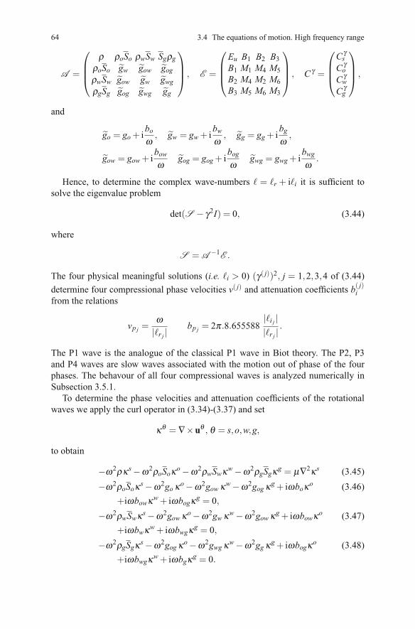
64
A =
⎛⎜⎜⎝ρ ρoSo ρwSw Sgρg
ρoSo gw gow gogρwSw gow gw gwgρgSg gog gwg gg
⎞⎟⎟⎠ , E =
⎛⎜⎜⎝Eu B1 B2 B3
B1 M1 M4 M5B2 M4 M2 M6B3 M5 M6 M3
⎞⎟⎟⎠ , C γ =
⎛⎜⎜⎝C γs
C γo
C γw
C γg
⎞⎟⎟⎠ ,
and
go = go+ iboω, gw = gw+ i
bwω
, gg = gg+ ibgω,
gow = gow+ ibowω
gog = gog+ ibogω
gwg = gwg+ ibwgω
.
Hence, to determine the complex wave-numbers = r + ii it is sufficient tosolve the eigenvalue problem
det(S − γ2I) = 0, (3.44)
where
S = A−1
E .
The four physical meaningful solutions (i.e. i > 0) (γ( j))2, j = 1,2,3,4 of (3.44)
determine four compressional phase velocities v( j) and attenuation coefficients b( j)ifrom the relations
vp j =ω|r j |
bp j = 2π.8.655588|i j ||r j |
.
The P1 wave is the analogue of the classical P1 wave in Biot theory. The P2, P3and P4 waves are slow waves associated with the motion out of phase of the fourphases. The behavour of all four compressional waves is analyzed numerically inSubsection 3.5.1.
To determine the phase velocities and attenuation coefficients of the rotationalwaves we apply the curl operator in (3.34)-(3.37) and set
κθ = ∇×uθ , θ = s,o,w,g,
to obtain
−ω2ρκs−ω2ρoSoκo−ω2ρwSwκw−ω2ρgSgκg = μ∇2κs (3.45)
−ω2ρoSoκs−ω2go κo−ω2gow κw−ω2gog κg+ iωboκo (3.46)
+iωbowκw+ iωbogκg = 0,
−ω2ρwSwκs−ω2gow κo−ω2gw κw−ω2gow κg+ iωbowκo (3.47)
+iωbwκw+ iωbwgκg = 0,
−ω2ρgSgκs−ω2gog κo−ω2gwg κw−ω2gg κg+ iωbogκo (3.48)
+iωbwgκw+ iωbgκg = 0.
3.4 The equations of motion. High frequency range

3 A poroelastic solid saturated by a three-phase fluid 65
Consider a plane rotational wave of angular frequency ω and wave number =r+ ii travelling in the x1-direction in the form
κs = As ei(x1−ωt), κo = Ao e
i(x1−ωt), (3.49)
κw = Aw ei(x1−ωt), κg = Ag e
i(x1−ωt)
Substitution of (3.49) in (3.46)-(3.48) yields the relations
−ω2ρoSoAs−ω2go Ao−ω2gowAw−ω2gog Ag+ iωboAo (3.50)
+iωbowAw+ iωbogAg = 0
−ω2ρwSwAs−ω2gowAo−ω2gwAw−ω2gwg Ag+ iωbowAo (3.51)
+iωbwAw+ iωbwgAg = 0
−ω2ρgSgAs−ω2gog Ao−ω2gwg Aw−ω2gg Ag+ iωbogAo (3.52)
+iωbwgAw+ iωbgAg = 0
Next, from (3.50)-(3.52), we can determine the amplitudes Ao,Aw,Ag as linear func-tions of the amplitude As in the form
Ao =CoAs, Aw =CwAs, Ag =CgAs, (3.53)
where the coefficients Co,Cw,Cg depend on the mass and viscous coupling coeffi-cients in (3.50)-(3.52). Next, using (3.49) in (3.45) and using (3.53) and (3.43) weget the equation
ρ +ρoSoCo+ρwSwCw+ρgSgCg =1γ2 μ . (3.54)
The physically meaningful solution of (3.54) gives the shear phase velocity andattenuation coefficient as
vs =ω|r| bs = 2π.8.655588
|i||r| .
3.5 Numerical Examples
In this section we compute phase velocities and attenuation coefficients for a sampleof Nivelsteiner sandstone saturated by a three phase fluid, taken to be oil, water andgas, water assumed to be the wetting phase. The material properties of the Nivel-steiner sandstone are given in Table 1.1.
The gas properties correspond to a dry gas at a reference pressure of 5MPa, (at adepth of 500 m, approximately ).

66
The capillary pressure functions Pcow(So) and Pcgo(Sg) used to determine theelastic coefficients are [Ravazzoli et al., 2003]
Pcow(So) = Aow(1/(So+Srw−1)2 −S2
ro/[So(1−Sro−Srw)]2) ,
Sro ≤ So ≤ 1−Srw−Srg,
Pcgo(Sg) = Aog(1/(Sg+Sro−1)2 −S2
rg/[Sg(1−Srg−Sro)]2) ,
Srg ≤ Sg ≤ 1−Sro−Srw.
In the examples we use Srw = Sro = Srg= 0.02, Aow = 40 kPa, Aog = 30 kPa.Besides, the relative permeability functions krθ (Sθ ),θ = o,w,g, are [Baker, 1988]
Krθ (Sθ ) =
(Sθ −Srθ1−Srθ
)2
,
Srθ ≤ Sθ ≤ 1−Srp−Srq, p = θ ,q = θ , p = q.
We used ε = 0.01 in the definitions of the cross mass and viscous coupling coef-ficients in (3.19)-(3.20) and (3.28)-(3.29).
3.5.1 Characterization of the four compressional modes ofpropagation
First we analyze the different compressional modes of propagation. As for singleand two-phase fluids, it is convenient to rewrite the equations of motion in terms ofthe solid and absolute fluid phases uo, uw and ug.
Seteq = ∇ · uq, q= o,w,g.
Using (3.4) in (3.21)- (3.24), taking divergence in the resulting equations and replac-ing a plane compressional wave of angular frequency ω and (real) wave number travelling in the x1–direction of the form
es = C()s ei(x1−ω
t), eo = C()o ei(x1−ω
t),
ew = C()w ei(x1−ω
t), eg = C()g ei(x1−ω
t),
leads to the eigenvalue problem
γ2A C() = E C(γ),
where γ is defined in (3.43), C γ =(C γs ,C
γo ,C
γw,C
γg
)tand
3.5 Numerical Examples

3 A poroelastic solid saturated by a three-phase fluid 67
A =
⎛⎜⎜⎝ρ −φ(ρoSo+ρwSw+ρgSg) φρoSo φρwSw φρgSg
ρoSo−φ(gco+gcow+gcog) φgco φgcow φgcogρwSw−φ(gcw+gcow+gcwg) φgcow φgcw gcwgρgSg−φ(gcog+gcwg+gcg) φgcog φgcwg gcg
⎞⎟⎟⎠ ,
E =
⎛⎜⎜⎝Eu−φ(B1 +B2 +B3) φB1 φB2 φB3
B1 −φ(M1 +M4 +M5) φM1 φM4 φM5B2 −φ(M2 +M4 +M6) φM4 φM2 φM6B3 −φ(M3 +M5 +M6) φM5 φM6 φM3
⎞⎟⎟⎠ .
The matrices Ci, i = 1, · · · ,6 in (3.55)-(3.57) illustrate symbolically the six pos-sibly cases in which the four phases can move.
Column j in these matrices shows the signs of the components of the eigenvectorsassociated with the phase velocities v( j), j = 1,2,3,4 ordered in decreasing order.The symbols s,o,w,g in the first column of these matrices indicate the componentsof each column eigenvector associated with the solid, oil, water and gas phases,respectively.
These results were obtained numerically for random choices of the values ofsaturations of the wetting and non-wetting fluids and reference wetting pressure pw.If, as in the capillary relations, the oil, water and gas are taken in pairs (o,w) and(g,o), from (3.55)-(3.57) we can see that there are four different ways in that the oil,water and gas can move:
• a)(o,w) in phase, (g,o) in phase (column 1 in matrices Ci, i= 1, · · · ,6).• b) (o,w) in phase, (g,o) in opposite phase (column 2 in matricesC1,C3,C4,C5,C6
and column 3 in matrix C2).• c)(o,w) in opposite phase, (g,o) in phase (column 3 in matrices C2,C3, column
4 in matrices C4,C5,C6).• d) (o,w) in opposite phase, (g,o) in opposite phase (column 4 in matricesC1,C2).
The numerical results shown in (3.55)-(3.57) allow us to conclude that:
• P1 waves: the solid moves in phase with the fluids as in case a). This is the fastcompressional wave in the classical Biot theory. The P1 wave is represented incolumn 1 of Ci, i= 1, · · · ,6.
• P2 waves: the solid moves in opposite phase with the fluids as in case a). Thisis the analogue of the slow Biot wave for single-phase fluids. The P2 wave isrepresented in column 3 of C1,C2 and column 2 of C3,C4,C5,C6.
• P3 waves: the solid moves in phase or opposite phase with the fluids as in case b).The P3 wave is represented in column 2 of C1,C2 and column 3 of C3,C4,C5,C6.
• P4 waves: the solid moves in phase or opposite phase with the fluids as in casesc) or d). The P4 wave is represented in column 4 of Ci, i= 1, · · · ,6.
This analysis also shows that depending on the value of the reference pressure pwand the saturation values of the fluid phases the P3 wave may have a faster velocitythan the P2 wave and the P4 wave is the slowest of the three slow waves.

68
C1 =
⎡⎢⎢⎢⎢⎣v(1) v(2) v(3) v(4)
s + − − −o + − + −w + − + +g + + + +
⎤⎥⎥⎥⎥⎦ , C2 =
⎡⎢⎢⎢⎢⎣v(1) v(2) v(3) v(4)
s + + − −o + − + −w + − + +g + + + +
⎤⎥⎥⎥⎥⎦ , (3.55)
C3 =
⎡⎢⎢⎢⎢⎣v(1) v(2) v(3) v(4)
s + − + −o + + − −w + + − +g + + + −
⎤⎥⎥⎥⎥⎦ , C4 =
⎡⎢⎢⎢⎢⎣v(1) v(2) v(3) v(4)
s + − − −o + + + −w + + + +g + + − −
⎤⎥⎥⎥⎥⎦ (3.56)
C5 =
⎡⎢⎢⎢⎢⎣v(1) v(2) v(3) v(4)
s + − − +o + + + +w + + + −g + + − +
⎤⎥⎥⎥⎥⎦ , C6 =
⎡⎢⎢⎢⎢⎣v(1) v(2) v(3) v(4)
s + − + +o + + − +w + + − −g + + + +
⎤⎥⎥⎥⎥⎦ (3.57)
3.5.2 Behaviour of all waves in the purely elastic case
Next let us analyze the behaviour of all waves for the non-dissipative case (zero vis-cosity) and several values of the reference pressure pw. The corresponding gas prop-erties for the different pressures, computed using the calculations in [Standing, 1977]and [McCoy, 1983] are given in Table 3.1.
Table 3.1 Properties of the gas phase as function of pressure
5 MPa bulk modulus, Kg 44515183.855×10−10 GPadensity, ρg 42.156366 kg/m3
viscosity, ηg 1.1186139×10⁻⁵ Pa · s
10 MPa bulk modulus, Kg 89314762.7 ×10−10 GPadensity, ρg 86.5156181 kg/m3
viscosity, ηg 1.17348206×10⁻⁵ Pa · s
20 MPa bulk modulus, Kg 229138783.0 ×10−10 GPadensity, ρg 151.545384 kg/m3
viscosity, ηg 1.28131716 ×10⁻⁵ Pa · s
30 MPa bulk modulus, Kg 408195703.0 ×10−10 GPadensity, ρg 185.844062 kg/m3
viscosity, ηg 1.38663132 ×10⁻⁵ Pa · s
3.5 Numerical Examples

3 A poroelastic solid saturated by a three-phase fluid 69
Figures 3.1 and 3.2 show phase velocities of all waves for the zero viscositycase as function of gas saturation at water saturation Sw = 0.25 and reference waterpressures pw equal to 20 and 30 MPa.
0 0,1 0,2 0,3 0,4 0,5 0,6Gas Saturation
2540
2550
2560
2570
2580
2590
Typ
e I
P-W
ave
Phas
e V
eloc
ity (
m/s
)
Type I, pw=20 MPa, Sw=0.25Type I, pw=30 MPa, Sw=0.25
1490
1500
1510
1520
1530
1540
1550
Shea
r W
ave
Phas
e V
eloc
ity (
m/s
)S-wave, pw=20 MPa, Sw=0.25S-wave, pw=30 MPa, Sw=0.25
P1
P1,P1,
Fig. 3.1 P1 and shear wave phase velocities as function of gas saturation at water saturation Sw =0.25 and reference water pressures pw = 20 and 30.
Figure 3.1 shows that P1 waves have higher velocities for higher values of pw,displaying a characteristic decreasing behaviour as gas saturation increases until athreshold value (which depends on pw) at which velocities start to increase. Thisbehaviour is similar to that observed in Figure 2.1 for the gas-water case.
Besides, phase velocities of S-waves are increasing functions of gas saturation,and show lower values for higher values of pw. Thus these fast P and S waves ve-locities mimic the behaviour of the corresponding Gassmann velocities.
Figure 3.2 shows a decrease of the P2 and P3 waves as gas saturation increases,behaving as the P2 wave for the gas-water case in Figure 2.2. Besides, they exhibithigher values for increasing values of pw. Also, P4 waves phase velocities are almostindependent of gas saturation and pw.
3.5.3 Behaviour of all waves as function of frequency
Next we analyze the behaviour of all waves as function of frequency fixing thesaturation of oil, water and gas as indicated in the different figures.
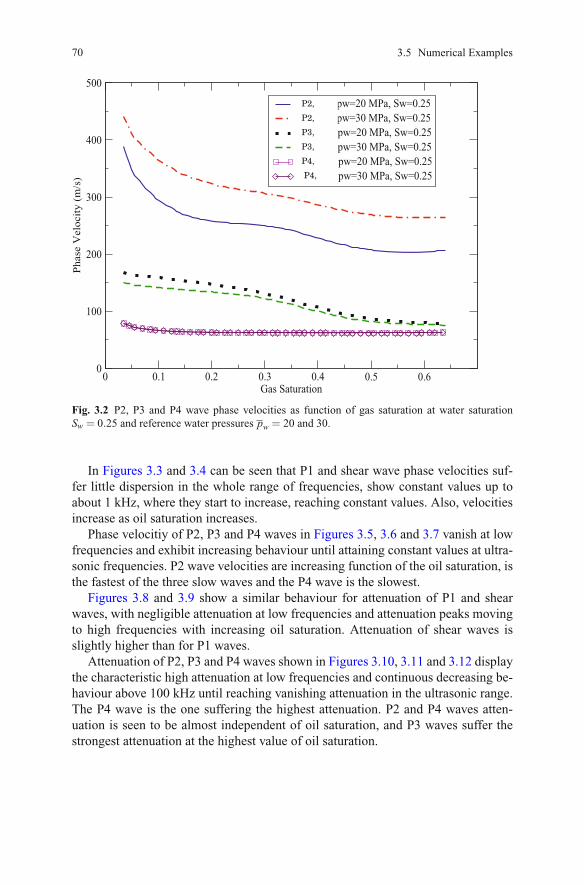
70
0 0.1 0.2 0.3 0.4 0.5 0.6Gas Saturation
0
100
200
300
400
500P
hase
Vel
ocit
y (m
/s)
Type II, pw=20 MPa, Sw=0.25Type II, pw=30 MPa, Sw=0.25Type III, pw=20 MPa, Sw=0.25Type III, pw=30 MPa, Sw=0.25Type IV, pw=20 MPa, Sw=0.25Type IV, pw=30 MPa, Sw=0.25
P2,
P2,
P3,
P3,
P4,
P4,
Fig. 3.2 P2, P3 and P4 wave phase velocities as function of gas saturation at water saturationSw = 0.25 and reference water pressures pw = 20 and 30.
In Figures 3.3 and 3.4 can be seen that P1 and shear wave phase velocities suf-fer little dispersion in the whole range of frequencies, show constant values up toabout 1 kHz, where they start to increase, reaching constant values. Also, velocitiesincrease as oil saturation increases.
Phase velocitiy of P2, P3 and P4 waves in Figures 3.5, 3.6 and 3.7 vanish at lowfrequencies and exhibit increasing behaviour until attaining constant values at ultra-sonic frequencies. P2 wave velocities are increasing function of the oil saturation, isthe fastest of the three slow waves and the P4 wave is the slowest.
Figures 3.8 and 3.9 show a similar behaviour for attenuation of P1 and shearwaves, with negligible attenuation at low frequencies and attenuation peaks movingto high frequencies with increasing oil saturation. Attenuation of shear waves isslightly higher than for P1 waves.
Attenuation of P2, P3 and P4 waves shown in Figures 3.10, 3.11 and 3.12 displaythe characteristic high attenuation at low frequencies and continuous decreasing be-haviour above 100 kHz until reaching vanishing attenuation in the ultrasonic range.The P4 wave is the one suffering the highest attenuation. P2 and P4 waves atten-uation is seen to be almost independent of oil saturation, and P3 waves suffer thestrongest attenuation at the highest value of oil saturation.
3.5 Numerical Examples

3 A poroelastic solid saturated by a three-phase fluid 71
Next, we study the sensibility of phase velocities of slow waves to changes inthe reference water pressure pw , taken to be 5, 10 and 20 MPa. The saturation ofthe three phases are Sw = 0.4,So = 0.5 and Sg = 0.1. Figures 3.13, 3.14 and 3.15show that their velocities increase as pw increases and stabilize at high frequencies.Concerning the high frequency values of the slow waves. P2 phase velocities arealmost independent of the reference water pressure pw. On the contrary, P3 and P4phase velocities show a strong dependency of oil saturation, that can be explainedby the way in which the fluid phases move in these two modes.
Attenuation of the fast P1 and shear waves are almost independent of pw and arenot shown.
Fig. 3.3 Phase velocity ofP1 waves as function offrequency for a sample ofNivelsteiner sandstone withwater saturation Sw = 0.1, oilsaturation So = 0.8 and gassaturation Sg = 0.1
-1 0 1 2 3 4 5 6 7Frequency (Hz) - Logarithmic Scale
2425
2450
2475
2500
2525
2550
P1 W
ave
Phas
e V
eloc
ity (
m/s
)
Sw = 0.1, So = 0.8Sw = 0.4, So = 0.5Sw = 0.8, So = 0.1
Fig. 3.4 Phase velocity ofshear waves as function offrequency for a sample ofNivelsteiner sandstone withwater saturation Sw = 0.1, oilsaturation So = 0.8 and gassaturation Sg = 0.1
-1 0 1 2 3 4 5 6 7Frequency (Hz) - Logarithmic Scale
1475
1500
1525
1550
Shea
r W
ave
Phas
e V
eloc
ity (
m/s
)
Sw = 0.1_So = 0.8Sw = 0.4, So = 0.5Sw = 0.8, So = 0.1

72
Fig. 3.5 Phase velocity ofP2 waves as function offrequency for a sample ofNivelsteiner sandstone withwater saturation Sw = 0.1, oilsaturation So = 0.8 and gassaturation Sg = 0.1
-1 0 1 2 3 4 5 6 7Frequency (Hz) - Logarithmic Scale
0
50
100
150
200
250
P2 W
aves
Pha
se V
eloc
ity (
m/s
) Sw = 0.1, So = 0.8Sw = 0.4, So = 0.5Sw = 0.8, So = 0.1
Fig. 3.6 Phase velocity ofP3 waves as function offrequency for a sample ofNivelsteiner sandstone withwater saturation Sw = 0.1, oilsaturation So = 0.8 and gassaturation Sg = 0.1
-1 0 1 2 3 4 5 6 7Frequency (Hz) - Logarithmic Scale
0
50
100
150
P3 W
aves
Pha
se V
eloc
ity (
m/s
) Sw = 0.1, So = 0.8Sw = 0.4, So = 0.5Sw = 0.8, So = 0.1
Fig. 3.7 Phase velocity ofP4 waves as function offrequency for a sample ofNivelsteiner sandstone withwater saturation Sw = 0.1, oilsaturation So = 0.8 and gassaturation Sg = 0.1
-1 0 1 2 3 4 5 6 7Frequency (Hz) - Logarithmic Scale
0
10
20
30
40
50
P4 W
aves
Pha
se V
eloc
ity (
m/s
) Sw = 0.1, So = 0.8Sw = 0.4, So = 0.5Sw = 0.8, So = 0.1
3.5 Numerical Examples

Fig. 3.8 Attenuation of P1waves as function of fre-quency for a sample of Nivel-steiner sandstone with watersaturation Sw = 0.1, oil sat-uration So = 0.8 and gassaturation Sg = 0.1
-1 0 1 2 3 4 5 6 7Frequency (Hz) - Logarithmic Scale
0
0.1
0.2
0.3
0.4
0.5
P1 W
ave
Atte
nuat
ion
(dB
)
Sw = 0.1, So = 0.8Sw = 0.4, So = 0.5Sw = 0.8, So = 0.1
Fig. 3.9 Attenuation of shearwaves as function of fre-quency for a sample of Nivel-steiner sandstone with watersaturation Sw = 0.1, oil sat-uration So = 0.8 and gassaturation Sg = 0.1
-1 0 1 2 3 4 5 6 7Frequency (Hz) - Logarithmic Scale
0
0.1
0.2
0.3
0.4
0.5
Shea
r W
ave
Atte
nuat
ion
(dB
) Sw = 0.1, So = 0.8Sw = 0.4, So = 0.5Sw = 0.8, So = 0.1
3.6 Appendix 1. Determination of the elastic coefficients.Inclusion of linear viscoelasticity
Since the shear modulus μ is assumed to be known and equal to the shear modulusof the dry matrix, as explained in Chapter 1, to determine the coefficients in (3.12)-(3.15) it is sufficient to consider tensional changes Δτi j of the form
Δτ11 = Δτ22 = Δτ33 =13
Δτ =−Δ p, Δ p> 0, Δτi j = 0, i = j.
For these tensional changes, from (3.12) we get the relation
−Δ p= Ku es−Bo ξ o−Bw ξw−Bgξ g, (3.58)
3 A poroelastic solid saturated by a three-phase fluid 73

74
Fig. 3.10 Attenuation ofP2 waves as function offrequency for a sample ofNivelsteiner sandstone withwater saturation Sw = 0.1, oilsaturation So = 0.8 and gassaturation Sg = 0.1
-1 0 1 2 3 4 5 6 7Frequency (Hz) - Logarithmic Scale
0
10
20
30
40
50
60
P2 W
ave
Atte
nuat
ion
(dB
)
Sw = 0.1, So = 0.8Sw = 0.4, So = 0.5Sw = 0.8, So = 0.1
Fig. 3.11 Attenuation ofP3 waves as function offrequency for a sample ofNivelsteiner sandstone withwater saturation Sw = 0.1, oilsaturation So = 0.8 and gassaturation Sg = 0.1
-1 0 1 2 3 4 5 6 7Frequency (Hz) - Logarithmic Scale
0
10
20
30
40
50
60
P3 W
aves
atte
nuat
ion
(dB
)
Sw = 0.1, So = 0.8Sw = 0.4, So = 0.5Sw = 0.8, So = 0.1
with Ku = λu+23 μ .
Let Kθ and Cθ = 1/Kθ denote the bulk modulus and compressibility of the θ -fluid, respectively, θ = o,w,g,u.
Considering the gedanken closed compressibility test as in Chapter 1, since forthe closed system there is conservation of mass of the fluid phases, ξ θ = 0, θ =o,w,g, and from (3.58) we see that Ku is the Gassmann undrained bulk modulus ofour closed system, which is given by the relation: (see [Santos and Savioli, 2015])
Ku = KsKm+ΞKs+Ξ
, Ξ =K∗
f (Ks−Km)
φ(Ks−K∗f )
, (3.59)
where
3.6 Appendix 1. Determination of the elastic coefficients. Inclusion of linear viscoelasticity

Fig. 3.12 Attenuation ofP4 waves as function offrequency for a sample ofNivelsteiner sandstone withwater saturation Sw = 0.1, oilsaturation So = 0.8 and gassaturation Sg = 0.1
-1 0 1 2 3 4 5 6 7Frequency (Hz) - Logarithmic Scale
0
10
20
30
40
50
60
P4 W
aves
Atte
nuat
ion
(dB
)
Sw = 0.1, So = 0.8Sw = 0.4, So = 0.5Sw = 0.8, So = 0.1
Fig. 3.13 Phase velocityof P2 waves as function offrequency for a sample ofNivelsteiner sandstone atpw = 5,10 and 20 MPa withwater saturation Sw = 0.4, oilsaturation So = 0.5 and gassaturation Sg = 0.1
-1 0 1 2 3 4 5 6 7Frequency (Hz) - Logarithmic Scale
0
50
100
150
200
250
P2 W
ave
Phas
e V
eloc
ity (
m/s
) pw = 5 MPapw = 10 MPapw = 20 MPa
C∗f = 1/K∗
f =(γowSoCo+SwCw+ γgwSgCu
)/α, (3.60)
α =(So+βow−βgo−β ow
go
)γow+Sw−βow+
(Sg+βgo+β ow
go
)γgw,
γow = r1a22 − r2a12/(a11a22 −a12a21)
γgw = r2a11 − r1a12/(a11a22 −a12a21)
a11 = 1+CoSoPc′ow(So)(Sw+Sg),
a22 = 1+CuSgPc′go(Sg)(So+Sw),
a12 =−CuSoSgPc′ow(So),
a21 =−(1+CoSoSgPc′go(Sg)),
r1 = 1+CwSoSwPc′ow(So), r2 =CwSwSgPc
′go(Sg).
3 A poroelastic solid saturated by a three-phase fluid 75

76
Fig. 3.14 Phase velocityof P3 waves as function offrequency for a sample ofNivelsteiner sandstone atpw = 5,10 and 20 MPa withwater saturation Sw = 0.4, oilsaturation So = 0.5 and gassaturation Sg = 0.1
-1 0 1 2 3 4 5 6 7Frequency (Hz) - Logarithmic Scale
0
50
100
150
200
250
300
P3 W
ave
Phas
e V
eloc
ity (
m/s
) pw = 5 MPapw = 10 MPapw = 20 MPa
Fig. 3.15 Phase velocityof P4 waves as function offrequency for a sample ofNivelsteiner sandstone atpw = 5,10 and 20 MPa withwater saturation Sw = 0.4, oilsaturation So = 0.5 and gassaturation Sg = 0.1
-1 0 1 2 3 4 5 6 7Frequency (Hz) - Logaritmic Scale
0
20
40
60
80
P4 W
ave
Phas
e V
eloc
ity (
m/s
)
pw = 5 MPapw = 10 MPapw = 20 MPa
In (3.60) the expression for the undrained modulus Ku in (3.59) is formally iden-tical to that for the single phase and the two-phase immiscible cases as given inChapters 1 and 2. The remaining coefficients can be determined from the followingrelations [Santos and Savioli, 2015]
B1 = KuΘ[(So+βow+βw
ow
)γow− (βow+βw
ow)], (3.61)
B2 = KuΘ[Sw+βw
ow+ γow(βwgo−βw
ow
)−βwgoγgw
], (3.62)
B3 = KuΘ[γgw(Sg+βgo+βw
go+β owgo
)− γow(βgo+βw
go+β owgo
)]. (3.63)
M1 = [B1Ro+βow+βwow]/Qo, (3.64)
M2 =[B2Rw−
((1−κ1)βw
go−βwow
)]/Qw, (3.65)
M3 =[B3Rg+κ8
(βgo+β ow
go +βwgo
)]/Qg, (3.66)
3.6 Appendix 1. Determination of the elastic coefficients. Inclusion of linear viscoelasticity
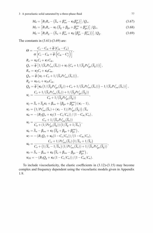
3 A poroelastic solid saturated by a three-phase fluid 77
M4 =[B2Ro−
(Sw+βw
ow−κ5βwgo
)]/Qo, (3.67)
M5 =[B3Ro−κ5
(Sg+βgo+β ow
go +βwgo
)]/Qo, (3.68)
M6 =[B2Rg−
(Sw+βw
ow+κ8(βwgo−βw
ow
))]/Qg. (3.69)
The constants in (3.61)-(3.69) are:
Θ =Cs−Cm+φ (Cm−Cu)
α[Cs−Cm+φ
(Cm−C∗
f
)] ,Ro = κ6Cs+κ7Cm,
Qo = φ[1/(SoPc′ow(So))+κ5
(Cu+1/(SgPc′go(Sg))
)],
Rw = κ2Cs+κ4Cm,
Qw = φ(κ3 +Co+1/(SoPc′ow(So))
),
Rg = κ9 cs+κ10Cm,
Qg = φ[κ8(1/(SgPc′go(Sg))+Co+1/(SoPc′ow(So))
)−1/(SoPc′ow(So))],
κ1 =Co+1/(SoPc′ow(So))+1/(SgPc′go(Sg))
Cu+1/(SgPc′go(Sg)),
κ2 = So+Sgκ1 +βow+(βgo+β ow
go
)(κ1 −1),
κ3 =(1/Pc′ow(So)+(κ1 −1)/Pc′go(Sg)
)/Sw
κ4 =−(B2Qw+κ2(1−Cs/Cu))/(1−Cm/Cu) ,
κ5 =Cw+1/(SwPc′ow(So))
Cu+(1/Pc′go(Sg))(1/Sg+1/Sw
) ,κ6 = Sw−βow+κ5
(Sg+βgo+β ow
go
),
κ7 =−(B1Qo+κ6(1−Cs/Cu))/(1−Cm/Cu),
κ8 =Cw+1/Pc′ow(So)
(1/Sw+1/So
)Co+
(1/So−1/Sw
)(1/Pc′ow(So))+1/(SwPc′go(Sg))
,
κ9 = Sw−βow+κ8(So+βow−βgo−β ow
go
),
κ10 =−(B3Qg+κ9 (1−Cs/Cu))/(1−Cm/Cu).
To include viscoelasticity, the elastic coefficients in (3.12)-(3.15) may becomecomplex and frequency dependent using the viscoelastic models given in Appendix1.9.

Chapter 4
Waves in a fluid-saturated poroelastic matrixcomposed of two weakly coupled solids
Abstract This chapter presents a theory to describe wave propagation in a porousmedium composed of two weakly coupled solids saturated by a single-phase fluid.The model is useful in realistic situations such as seismic wave propagation in per-mafrost or shaley sandstones. The constitutive relations are derived from the virtualwork principle, allowing to determine the generalized forces of the system and theconstitutive relations, given here for the isotropic case. The coefficients in the consti-tutive relations are defined for the cases of shaley sandstones and permafrost. Afterstating the equations of motion, including dissipative effects, a plane wave analysisreveals the existence of three compressional waves and two shear waves. The theoryis applied to determine phase velocities of the fast compressional and shear wavesin a sample of shaley sandstone, which are shown to fit experimental data.
4.1 Introduction
Wave propagation in composite porous materials has applications in many branchesof science and technology, such as seismic methods in the presence of shaleystones[Carcione et al., 2000], permafrost [Morack and Rogers, 1981, Carcione and
and gas-hydrate concentration in ocean-bottom sediments [Carcione
Here we present an extension of the Biot theory described in Chapter 1 to modelwave propagation in a porous medium composed of two weakly coupled solids sat-urated by a single-phase fluid.
This problem has been solved for the case of uniform porosity in [Leclaire et al., 1994]for describing wave propagation in frozen porous media in which solid substrate, iceand water coexist, under the assumption of the existence of a layer of unfrozen wateraround the solid particles isolating them from ice. This model predicts the existenceof three compressional waves, (P1,P2 and P3 waves) and two shear waves, (S1 andS2 waves). The P1 and S1 waves correspond to the case of all the phases moving inphase; the P2 wave corresponds to the classical slow Biot wave; the P3 and S2 waves
© Springer International Publishing AG 2016
in Geosystems Mathematics and Computing, DOI 10.1007/978-3-319-48457-0_4
79
sand-
Seriani, 1998]and Tinivella, 2000a].
J.E. Santos, P.M. Gauzellino, Numerical Simulation in Applied Geophysics, Lecture Notes

80
are associated with propagation modes in the solid phase accompanying matrix withinfinite permeability in the rock-frame or zero viscosity in the fluid phase.
The verification that additional (slow) waves can be observed in laboratory ex-periments was published in [Leclaire et al., 1985]. Later, this theory was extendedin [Carcione and Tinivella, 2000a] to include the interaction between the solid andice particles and grain cementation with decreasing temperature.
This Chapter presents a generalization to the case of non-uniform porosity of thetheory in [Leclaire et al., 1994, Carcione and Tinivella, 2000a]. This generalization,appeared in [Santos et al., 2004a], can be used to perform numerical experiments orfit laboratory data related to heterogeneous media.
As an application, we mention the work by [Rubino et al., 2008], where thismodel was used to analyze conversions to Biot-type slow waves in highly heteroge-neous gas-hydrate bearing sediments.
The non-welding condition between the two solid phases is assumed when defin-ing the potential and kinetic energies, with proper interaction terms among the solidand fluid phases. If the two solid phases would be welded, then additional slowwaves would not be present [Brown and Korriga, 1975].
The derivation is based on the energy formulation presented in Chapter 1, ratherthan on volume averaging or homogenization methods. A formal derivation of thismodel using homogenization techniques appeared in [Santos et al., 2005b].
4.2 The strain energy of the composite system
Let Ω be an elementary cube of porous material composed of two solid phases,referred to by the subscripts or superscripts 1 or (1) and 3 or (3), saturated by a fluidphase indicated by the subscript or superscript (2). Thus, Ω = Ω1 ∪Ω2 ∪Ω3.
Let Vi denote the volume of the phase Ωi and Vb and Vsm the bulk volume of Ωand the solid matrix Ωsm = Ω1 ∪Ω3, so that
Vsm =V1 +V3, Vb =V1 +V2 +V3.
Let S1 =V1
Vsmand S3 =
V3
Vsm, denote the two solid fractions of the composite matrix.
We also define the effective porosity as
φ =V2
Vb.
Let u(1), u(2) and u(3) be the averaged solid and fluid displacements over the bulkmaterial. Here u(2) is defined such that on any face F of the cube Ω∫
Fφu(2) ·ν dF
is the amount of fluid displaced through F , while
4.2 The strain energy of the composite system

4 Waves in a fluid-saturated poroelastic matrix composed of two weakly coupled solids 81∫FS1u(1) ·ν dF and
∫F
S3u(3) ·ν dF
represent the displacements in the two solid parts of F , respectively. Here ν denotesthe unit outward normal to F ,
Let σ (1)i j and σ (3)
i j denote the stress tensors in Ω1 and Ω3 averaged over the bulkmaterial Ω , respectively, and let p f denote the fluid pressure. These quantities de-
scribe small changes with respect to reference values σ (1)i j ,σ
(3)i j and p f correspond-
ing to an initial equilibrium state. Let us also introduce the tensors
σ (1,T )i j = σ (1)
i j −S1φ p f δi j, σ (3,T )i j = σ (3)
i j −S3φ p f δi j, (4.1)
associated with the total stresses in Ω1 and Ω3, respectively, so that the total stresstensor in the bulk material Ω is given by
σi j = σ (1,T )i j +σ (3,T )
i j .
Next we shall derive the stress-strain relations for our system using the virtualwork principle, following the derivation for the case of a single solid phase given inChapter 1.
Let W be the strain energy density and V the total potential energy. Also letVd denote the total potential energy density. Then, if f (1)i , f (3)i , f (2)i represent thesurface forces acting on the solid and fluid parts of the boundary of Ω , denoted by∂Ω , we have that
V =∫
ΩVd dΩ =
∫Ω
W dΩ −∫
∂Ω( f (1)i u(1)i + f (2)i u(2)i + f (3)i u(3)i )d(∂Ω),
and the virtual work principle for the composite fluid-solid system can be stated inthe form:
δV = 0 =
∫Ω
δW dΩ −∫
∂Ω( f (1)i δ (u(1)i )+ f (2)i δ (u(2)i )+ f (3)i δu(3)i )d(∂Ω), (4.2)
wheref (1)i = σ (1)
i j ν j, f (3)i = σ (3)i j ν j, f (2)i =−φ p f δi jν j, (4.3)
and δ denotes virtual changes in the different quantities. Using (4.3) in (4.2) we get
δV = 0 =∫
ΩδW dΩ −
∫∂Ω
(σ (1,T )i j ν jδ (u
(1)i )+σ (3,T )
i j ν jδ (u(3)i ) (4.4)
−p f δi jν jδwi
)d(∂Ω).
wherewi = φ
(u(2)i −S1u
(1)i −S3u
(3)i
). (4.5)
Then, transforming the surface integral in (4.4) into a volume integral we get

82
δV = 0 =∫
ΩδW dΩ −
∫Ω
∂∂x j
[σ (1,T )i j δ (u(1)i )+σ (3,T )
i j δ (u(3)i )
−p f δi jδwi]dΩ .
Since Ω remains in equilibrium under the action of the virtual displacements, wehave that
∂∂x j
σ (1,T )i j =
∂∂x j
σ (3,T )i j =
∂∂x j
p f δi j = 0,
and consequently, using the symmetry of the stress tensors σ (1,T )i j and σ (3,T )
i j weobtain
δV = 0 =∫
ΩδW dΩ −
∫Ω
(σ (1,T )i j δ (εi j(u(1)))+σ (3,T )
i j δ (εi j(u(3)))
+p f δζ)dΩ ,
where
ζ =−∇ ·w
represents the change in fluid content and εi j(u(m)),m = 1,3 is the strain tensor inΩm with linear invariant e(m) = εii(u(m)).
Thus from (4.1) we finally obtain the following expression for the variation instrain energy density δW :
δW = (σ (1)i j −S1φ p f δi j)δ (εi j(u(1)))+(σ (3)
i j −S3φ p f δi j)δ (εi j(u(3))) (4.6)
+p f δζ
= σ (1,T )i j δ (εi j(u(1)))+σ (3,T )
i j δ (εi j(u(3)))+ p f δζ .
Consequently, since δW is an exact differential of the variables εi j(u(1)), εi j(u(3))and ζ we have that
∂W
∂εi j(u(1))= σ (1,T )
i j = σ (1)i j −S1φ p f δi j,
∂W
∂εi j(u(3))= σ (3,T )
i j = σ (3)i j −S3φ p f δi j,
∂W
∂ζ= p f .
Also, it follows from (4.6) that
W =12
[(σ (1)
i j −S1φ p f δi j)(εi j(u(1)))+(σ (3)i j −S3φ p f δi j)(εi j(u(3))) (4.7)
+p f ζ].
4.2 The strain energy of the composite system

4 Waves in a fluid-saturated poroelastic matrix composed of two weakly coupled solids 83
4.3 Constitutive relations
Let us denote the deviatoric strain tensor in Ωm as
d(m)i j = εi j(u(m))− 13e(m)δi j, m= 1,3.
In the linear isotropic case the strain energy density W in (4.7) is a quadratic positivedefinite form in the invariants e(1), e(3), ζ , (d1)
2 = d(1)i j d(1)i j , (d3)2 = d(3)i j d(3)i j and
d1,3 = d(1)i j d(3)i j . Note that
(d1)2 = εi j(u(1)) εi j(u(1))− 1
3(e(1))2, (d3)
2 = εi j(u(3)) εi j(u(3))− 13(e(3))2,
and
d1,3 = εi j(u(1)) εi j(u(3))− 13e(1)e(3).
Then,
W =12E1(e
(1))2 +μ1(d1)2 +
12E3(e
(3))2 +μ3(d3)2
−B1e(1)ζ −B2e(3)ζ +B3e(1)e(3) +12M(ζ )2 +μ1,3d1,3.
The B3 and μ13 terms represent elastic interaction between the two solid phases.Thus, we obtain
∂W
∂εi j(u(1))= σ (1,T )
i j = σ (1)i j −S1φ p f δi j (4.8)
=[E1e
(1)−B1ζ +B3e(3)]δi j+2μ1d
(1)i j +μ1,3d
(3)i j ,
∂W
∂εi j(u(3))= σ (3,T )
i j = σ (3)i j −S3φ p f δi j (4.9)
=[E3e
(3)−B2ζ +B3e(1)]δi j+2μ3d
(3)i j +μ1,3d
(1)i j ,
∂W
∂ζ= p f =−B1e
(1)−B2e(3) +Mζ . (4.10)
Equations (4.8)-(4.9)-(4.10) express the generalized stressesσ (1,T )i j =σ (1)
i j −S1φ p f δi j,σ (3,T )i j σ (3)
i j −S3φ p f δi j and p f in terms of the strains εi j(u(1)),εi j(u(3)) and ζ .=

84
4.4 Determination of the coefficients in the constitutive relations
In this section we present a procedure to determine the coefficients in the stress-strain relations (4.8)-(4.9)-(4.10). The moduli for the case of uniform porosity can beobtained from known expressions given in a previous formulation [Carcione and
for the constant porosity case.First note that setting
θ2 = ∇ ·u(2) , θ3 = ∇ ·u(3)
for the case of uniform porosity from (4.5) we have that
ζ = φ(S1θ1 +S3θ3 −θ2) (4.11)
and consequently, from (4.10) we get
−φ p f = (B1φ −Mφ 2S1)θ1 +(B2φ −Mφ 2S3)θ3 +Mφ 2θ2. (4.12)
Next, combining (4.8), (4.11) and (4.12) we obtain
σ (1)i j =
[E1 +(S1φ)2M−2S1φB1
]θ1 + (4.13)[
S1S3φ 2M−S3φB1 −S1φB2 +B3
]θ3
−(φ 2S1M−φB1)θ2
δi j+2μ1d
(1)i j +μ1,3d
(3)i j .
Also, from (4.9), (4.11) and (4.12) we see that
σ (3)i j =
[E3 +(S3φ)2M−2S3φB2
]θ3 + (4.14)[
S3S1φ 2M−S3φB1 −S1φB2 +B3
]θ1
−(φ 2S3M−φB2)θ2
δi j+2μ3d
(3)i j +μ1,3d
(1)i j .
Set
K2 = Mφ 2,
C12 = B1φ −Mφ 2S1,
C23 = B2φ −Mφ 2S3,
K1 = E1 +(S1φ)2M−2S1φB1, (4.15)
K3 = E3 +(S3φ)2M−2S3φB2,
C13 = S1S3φ 2M−S3φB1 −S1φB2 +B3.
Tinivella, 2000a]
4.4 Determination of the coefficients in the constitutive relations

4 Waves in a fluid-saturated poroelastic matrix composed of two weakly coupled solids 85
Then, for constant porosity, the stress-strain relations (4.12)-(4.14) can be statedas follows:
σ (1)i j = (K1θ1 +C13θ3 +C12θ2)δi j+2μ1d
(1)i j +μ1,3d
(3)i j , (4.16)
σ (3)i j = (K3θ3 +C13θ1 +C23θ2)δi j+2μ3d
(3)i j +μ1,3d
(1)i j , (4.17)
−φ p f = C12θ1 +C23θ3 +K2θ2. (4.18)
Relations (4.16)-(4.18) were derived in [Leclaire et al., 1994] for the case of uni-form porosity and when the solid phase 3 is ice; it is also assumed in [Leclaire et al.,
C13 = μ1,3 = 0.The nonsingular linear system of equations (4.15) relating the coefficients for
both formulations can always be solved to obtain expressions for the coefficientsof the variable porosity formulation in terms of the corresponding to the uniformporosity case, with the following expressions:
E1 = K1 +(S1)2K2 +2S1C12,
E3 = K3 +(S3)2K2 +2S3C23,
B1 =S1K2 +C12
φ, (4.19)
B2 =S3K2 +C23
φ,
B3 =(C13 +S3C12 +S1C23 +S3S1K2
),
M =K2
φ 2 .
In Appendix 4.8 we give the formulas for the computation of the coefficientsK1, K2, K3, C12, C13, C23, μ1,μ3,μ1,3, which combined with (4.19) allows for theevaluation of the moduli H1, H3, B1, B2, B3, M, needed for this variable porosityformulation.
4.4.1 Inclusion of linear viscoelasticity
To introduce viscoelasticity we use the correspondence principle stated by M. Biot[Biot, 1962], i.e. we replace the real poroelastic coefficients in the constitutive rela-tions by complex frequency dependent poroviscoelastic moduli satisfying the samerelations as in the elastic case. In this work we use the linear viscoelastic model con-sisting in a continuous superposition of Zener elements as described in Appendix1.9 to make the set of moduli KG1,KG3,μ1,μ3,μ1,3 and B3 (see (4.34) in Appendix4.8 for the definition of KG1 and KG3) complex and frequency dependent, while allother coefficients in the constitutive relations remain real.
1994] that there is no contact between the solid and ice phases. This situation corres-ponds to the particular case in which

86
4.5 The equations of motion
The derivation of the kinetic energy and dissipation function densities is given in[Santos et al., 2004a], leading to the following formulation of the equations of mo-tion:
m11u(1)i +m12wi+m13u
(3)i + f11u
(1)i − f12wi− f11u
(3)i
− ∂∂x j[σ (1)i j −S1φ p f δi j
]= f (1)i , (4.20)
m12u(1)i +m22wi+m23u
(3)i − f12u
(1)i + f22wi+ f12u
(3)i
+∂ p f
∂xi= f (2)i , (4.21)
m13u(1)i +m23wi+m33u
(3)i − f11u
(1)i + f12wi+ f11u
(3)i
− ∂∂x j[σ (3)i j −S3φ p f δi j
]= f (3)i , i= 1,2,3, (4.22)
where f (1)i , f (2)i and f (3)i are external sources.The mass coupling coefficients in (4.20)–(4.22) are given by
m11 = ρ2φ +(φ)2((S3)
2m(1,2) + (S1)2m(3,2)
)−2S3ρ2φ
−(S1)2ρ2φ +(φ1)
2n(1,3) + (φ3)2n(3,1)−φ3ρ3,
m12 = p21 = ρ2 +φ(S1m
(3,2)−S3m(1,2))−S1ρ2,
m13 = p31 = ρ2φ − (φ)2((S3)
2m(1,2) + (S1)2m(3,2)
)−S1S3ρ2φ (4.23)
+ρ1φ1 − (φ1)2n(1,3) +ρ3φ3 − (φ3)
2n(3,1),
m22 = m(1,2) +m(3,2)− ρ2
φ,
m23 = p32 = ρ2 +φ(S3m
(1,2)−S1m(3,2))−S3ρ2,
m33 = ρ2φ +(φ)2((S3)
2m(1,2) + (S1)2m(3,2)
)−2S1ρ2φ
−(S3)2ρ2φ +(φ1)
2n(1,3) + (φ3)2n(3,1)−φ1ρ1.
The coefficientsmi j in (4.23) can be written in terms of the tortuosities a13, a31, a12,and a32 defined in Refs. [Carcione and Tinivella, 2000a] and [Leclaire et al., 1994]as follows:
n(1,3) = a13ρ1
φ1, n(3,1) = a31
ρ3
φ3, (4.24)
m(1,2) = a12ρ2
φ, m(3,2) = a32
ρ2
φ,
4.5 The equations of motion

4 Waves in a fluid-saturated poroelastic matrix composed of two weakly coupled solids 87
a12 =φ1ρφρ2
r12 +1, a32 =φ3ρ ′
φρ2r32 +1,
a13 =φ3ρ ′
φ1ρ1r13 +1, a31 =
φ1ρφ3ρ3
r31 +1,
where ri j are the geometrical aspects of the boundaries separating the phases i andj (equal to 1
2 for spheres) and
ρ =φρ2 +φ3ρ3
φ +φ3, ρ ′ =
φρ2 +φ1ρ1
φ +φ1.
Using the relations (4.24) in (4.23) we get
m11 = ρ2φ(1+(S1)
2a32 +(S3)2a12 −2S3 − (S1)
2)+a13ρ1φ1 +(a31 −1)ρ3φ3,
m12 = ρ2 (1+S1(a32 −1)−S3a12) ,
m13 = ρ2φ(1− (S1)
2a32 − (S3)2a12 −S1S3
)+ρ1φ1(1−a13)+ρ3φ3(1−a31),
m22 =ρ2
φ(a12 +a32 −1) ,
m23 = ρ2 (1+S3(a12 −1)−S1a32) ,
m33 = ρ2φ(1+(S1)
2a32 +(S3)2a12 −2S1 − (S3)
2)+a31ρ3φ3 +(a13 −1)ρ1φ1.
The expressions for the dissipation coefficients f11, f22 and f12 in (4.20)–(4.22)are determined as follows.
For the case of frozen porous media, following [Carcione and Tinivella, 2000a],we define the dissipation coefficients b12,b23 and b13 as
b12 = (φ)2 ηκ1
, b23 = (φ)2 ηκ3
,
while b13 is a friction coefficient between the ice and the solid frames. Also, ηdenotes the fluid viscosity and the permeability coefficients κ1,κ3 are defined interms of the absolute permeabilities κ1,0, κ3,0 of the two solid frames by the relations(see also [Leclaire et al., 1994])
κ1 = κ1,0(φ)3
(1−φ1)3 , κ3 = κ3,0(1−φ1)
2
φ 23
(φφ1
)3
. (4.25)
For the case of shaley sandstones, following [Carcione et al., 2000] the coeffi-cient b13 can be assumed to be zero and the friction coefficients b12 and b23 aretaken to be of the form:
d12 = 45ηR−2s1 φ−1(1−φ)φ1, d23 = 45ηR−2
s3 φ−1(1−φ)φ3, (4.26)
where Rs1,Rs3 denote the average radii of the sand and clay particles, respectively.Next, the frequency independent friction coefficients for this model are given by

88
f11 = c11 +d13, f12 =d12S3 −d23S1
φ, f22 =
d12 +d23
φ 2 , (4.27)
where c11 = d12S23 +d23S2
1.
4.5.1 Correction of the viscodynamic coefficients in the highfrequency range
In the high frequency range the set of inertial and friction coefficients are modified asfollows. Let F(ω) = FR(ω)+ iFI(ω), be the frequency correction function definedin either (1.93) or (1.94) where the permeability is given by
1κ=
1κ1
+1κ3
.
Then we define the frequency dependent mass and viscous coupling coefficients inthe following fashion
m11(ω) = m11 +FI(ω)c11
ω, (4.28)
m12(ω) = m12 − FI(ω) f12
ω,
m13(ω) = m13 − FI(ω)c11
ω,
m22(ω) = m22 +FI(ω) f22
ω,
The coefficients d13 is left as a free parameter chosen so that the following conditionis satisfied
f11 f22 − f 212 ≥ 0. (4.29)
Since the coefficient b13 takes into account friction between the two solid phases,a proper model based for example in Coulomb’ s friction theory may be used. Forsimplicity in all the numerical examples we have set the coefficient b13 to be zero.
4.5 The equations of motion
m23(ω) = m23 +FI(ω) f12
ω,
m33(ω) = m33 +FI(ω)c11
ωf11(ω) = FR(ω) 11 +b13, f12(ω) =
f22(ω) = FR(ω) f22.
,
FR(ω) f12,f

4 Waves in a fluid-saturated poroelastic matrix composed of two weakly coupled solids 89
4.6 Plane wave analysis
To determine the different types of waves that can propagate in this type of media,we use the argument given in Chapter 1 assuming plane waves of angular frequencyω and wave number = r + ii travelling in the x1-direction and satisfying theequations of motion (4.20), (4.21) and (4.22).
The argument, (using the frequency dependent definition of the viscodynamic co-efficients in (4.28) in the high frequency range) leads to the solution of the followingeigenvalue problem
det(S − γ2I) = 0, (4.30)
whereγ =
ω,
S = A−1
E . (4.31)
The matrices A ∈ R7×7 and E ∈ R7×7 in (4.31) are defined by
A =
⎡⎢⎢⎢⎢⎢⎢⎢⎢⎣
m11 0 0 m12 m13 0 00 q1 0 0 0 q2 00 0 q1 0 0 0 q2
m12 0 0 m22 m33 0 0m13 0 0 m23 m33 0 0
0 q2 0 0 0 q3 00 0 q2 0 0 0 q3
⎤⎥⎥⎥⎥⎥⎥⎥⎥⎦,
and
E =
⎡⎢⎢⎢⎢⎢⎢⎢⎢⎣
E1 +43 μ1 0 0 B1 B3 +
23 μ13 0 0
0 μ1 0 0 0 12 μ13 0
0 0 μ1 0 0 0 12 μ13
B1 0 0 M B2 0 0B3 +
23 μ13 0 0 B2 E3 +
43 μ3 0 0
0 12 μ13 0 0 0 μ3 0
0 0 12 μ13 0 0 0 μ3
⎤⎥⎥⎥⎥⎥⎥⎥⎥⎦,
where
m11 = m11 − if11
ω, m12 = m12 + i
f12
ω, , m13 = m13 + i
f11
ω,
m22 = m22 − if22
ω, m23 = m23 − i
f12
ω, m33 = m33 − i
f11
ω,
q1 = m11 − (m12)2
m22, q2 = m13 − m12m23
m22, q3 = m33 − m2
23
m22.

90
After solving (4.30) for the complex eigenvalues (γ j)2, j = 1, · · · ,7 the phase veloc-ities v( j) and the attenuation coefficients b( j) (in dB) of the compressional and shearwaves are obtained in terms of γ j from the relations
v( j) =ω
|( j)r |, b( j) = 2π ·8.685889
|( j)i ||(s)j |
, j = 1, · · · ,7. (4.32)
Of the seven eigenvalues of the matrix S , three of them, associated with thefirst,fourth and fifth row and columns of S are related with the compressionalmodes, while of the other four eigenvalues, associated with the second, third, sixthand seventh rows and columns of S , only two of them are different and are relatedwith the two shear modes of propagation.
The slow wave modes are important to explain attenuation and dispersion effectsobserved on the faster modes associated with scattering phenomena due to the pres-ence of heterogeneities inside the composite poroelastic materials being analyzed.
4.7 Numerical Examples. Shaley sandstones
Let us consider a shaley sandstone, and denote the sand fraction by S1 and the clayfraction by S3. As stated previously, the theory predicts three compressional waves(P1, P2 and P3 waves) and two shear waves (S1 and S2 waves), whose phase veloc-ities can be obtained by solving the eigensystem resulting from the equation of mo-tion as indicated in Section 4.6 (cf. (4.30)-(4.32)); see also [Carcione et al., 2000].In this example, we consider the faster P and S waves.
The bulk and shear moduli of the sand and clay (dry) matrices versus porosityφ are obtained from a relationship proposed by [Krief et al., 1990] using formulas(4.35)–(4.36) in Appendix 4.8.3
We consider the data set published by [Han et al., 1986]. obtained at a confiningpressure of 40 MPa. Han and his co-workers provide ultrasonic measurements of P-and S-wave velocities for 75 sandstone samples with porosities ranging from 2 %to 30 % and clay content from 0 to 50 %. One feature of this data set is that a smallamount of clay significantly softens the rock moduli, leading to reduced velocities.Table I shows the properties of the different constituents.
The permeabilities and friction coefficients are calculated by using the equationsgiven in (4.25), (4.26) and (4.27)
Moreover, the geometrical aspects ri j of the boundaries separating the phases iand j needed in (4.24) to determine de the mass coefficients pi j in (4.23) were takento be r12 = r32 = r13 = r31 = 1/2.
The predictions of the theory against the measurements obtained by [Han et al.,are shown in Figure 4.1.
We used the values A = 2 and a = 0.5 to determine the moduli Ks1,m,Ks3,m andμs1,m in (4.35) and (4.36).
1986]
4.7 Numerical Examples. Shaley sandstones

4 Waves in a fluid-saturated poroelastic matrix composed of two weakly coupled solids 91
Table 4.1 Material properties of the clay-bearing sandstone
Solid grain bulk modulus, Ks1 39 GPashear modulus, μs1 39 GPadensity, ρ1 2650 kg/m3
average radius, Rs1 50 μm
Clay bulk modulus, Ks3 20 GPashear modulus, μs3 10. GPadensity, ρ3 2650 kg/m3
average radius, Rs3 1 μm
Fluid bulk modulus, Kf 2.4 GPadensity, ρ2 1000 kg/m3
viscosity, η 1.798 cP
A frequency of 5 kHz was assumed to fit the experimental data, without includingviscoelasticity. Strictly speaking, this is not correct since the data has been acquiredat ultrasonic frequencies of the order of hundreds of kilohertz, and Biot-type dis-sipation mechanisms alone do not account for the level of attenuation observed inrocks.
The figure shows the compressional and shear velocities versus porosity, whereeach curve corresponds to a different value of the clay content S3. The root-mean-square deviation computed for all samples, apart from five outliers for P waves andseven outliers for S waves, is 93 m/s for the P-wave velocity and 100 m/s for theS-wave velocity. This results reflects the robustness of the model for this particularexample.
4.8 Appendix 1. Calculation of the elastic coefficients in thestress-strain relations
In this section we indicate a form of evaluating the coefficients in the stress-strainrelations (4.16)–(4.18), which combined with (4.19) yield the values of the coeffi-cients for the variable porosity formulation.
Let Ks1,m,Ks3,m, μs1,m and μs3,m denote the bulk and shear modulus of thetwo solid (dry) frames, respectively. In Subsections 4.8.1 and 4.8.2 we indicatehow to determine these moduli for the two examples presented in this paper.Also, let Ks1,μs1,Ks3,μs3 denote the bulk and shear moduli of the grains in thetwo solid phases, respectively, and let Kf denote the bulk modulus of the fluidphase. For the coefficients μ1,μ3 and μ13 we use the formulas given in Ref.[Carcione and Tinivella, 2000a]:
μ1 = [(1−g1)φ1]2μav+μs1,m, (4.33)
μ3 = [(1−g3)φ3]2μav+μs3,m,

Fig. 4.1 Velocities of the faster compressional (a) and shear (b) waves versus porosity φ for differ-ent values of clay content S3, indicated by the numbers inside the boxes (1: S3 = 0%, 2: S3 = 10%,3: S3 = 20%, 4: S3 = 30% and 5: S3 = 40%). The experimental data, represented with numbers,correspond to the data set published by Han et al.[Han et al., 1986]. In this case, 1, 2, 3, 4 and 5correspond to S3 values in the ranges [S3,S3 +5%],S3 = 0, ..., 40 %. The frequency is 5 kHz.
92 4.8 Appendix 1. Calculation of the elastic coefficients in the stress-strain relations

4 Waves in a fluid-saturated poroelastic matrix composed of two weakly coupled solids 93
μ13 = (1−g1)(1−g3)φ1φ3μav,
g1 =μs1,m
φ1μs1, g3 =
μs3,m
φ3μs3,
μav =[ (1−g1)φ1
μs1+
φ2ωη
+(1−g3)φ3
μs3
]−1,
where g1 and g3 are the so called shear consolidation coefficients of the solid frames1 and 3 [Leclaire et al., 1994]. The symbol ω in the definition of μav above denotesthe angular frequency.
Also, since K2 = φ 2M, (cf. (4.15)), to determine K2 we use the following expres-sion for Kav given in Ref. [Carcione and Tinivella, 2000a]:
M =
[(1− c1)
φ1
Ks1+
φKf
+(1− c3)φ3
Ks3
]−1
.
The remaining elastic coefficients are given by the following expressions [Carcione
K1 = [(1− c1)φ1]2M+Ks1,m, K3 = [(1− c3)φ3]
2M+Ks3,m,
C12 = (1− c1)φ1φM, C13 = (1− c1)(1− c3)φ1φ3M, C23 = (1− c3)φφ3M,
c1 =Ks1,m
φ1Ks1, c3 =
Ks3,m
φ3Ks3,
where c1,c3 are the bulk consolidation coefficients of the solid frames 1 and 3.These elastic moduli for constant porosity can be rewritten as follows:
K1 = KG1 −2α1S1φM+(S1φ)2M,
K3 = KG3 −2α3S3φM+(S3φ)2M,
C12 = φM(α1 −S1φ),C23 = φM(α3 −S3φ),C13 =M(α1 −S1φ)(α3 −S3φ),
where
KG1 = Ks1,m+(α1)2M, KG3 = Ks3,m+(α3)
2M, (4.34)
α1 = S1 − Ks1,m
Ks1, α3 = S3 − Ks3,m
Ks3.
The moduli KG1 and KG3 are the analogous of the Gassmann’s modulus, while thecoefficients α1 and α3 correspond to the classic effective stress coefficients α in theclassic Biot theory.
The bulk and shear moduli Ks1,m,Ks3,m, μs1,m and μs3,m in (4.33) and (4.34) canbe determined in several fashions. In some cases, they can be obtained from themeasurements of compressional and shear wave velocities on the empty rock oralternatively, they can be estimated using known petrophysical models. Below we
and Tinivella, 2000a]

94
indicate the procedure used in this paper to determine those moduli for the cases ofshaley sandstones and frozen porous media presented in this paper.
4.8.1 The case of shaley sandstones
The porosity dependence of the sand and clay (dry) matrices is consistent with theconcept of critical porosity, since the moduli should vanish above a certain valueof the porosity (usually from 0.4 to 0.5). This dependence is determined by theempirical coefficient A in equation (4.35).
In some rocks there is an abrupt change of rock matrix properties with the ad-dition of a small amount of clay, attributed to softening of cements, clay swellingand surface effects. That is, the wave velocities decrease significantly when the claycontent increases from zero to a few percentages. In order to model this effect, wemultiply the shear modulus of the sand matrix by a factor depending on the empiri-cal coefficient a in equation (4.36) (this factor tends to 1 when a→ ∞).
If Ω1 represents the sand and Ω3 the clay minerals, then the bulk and shearmoduli of the sand and clay (dry) matrices are assumed to satisfy
Ks j,m = S jKs j(1−φ)1+A/(1−φ), j = 1,3, (4.35)
μs1,m = exp−[(1−S3)S3)]aKs1,mμs1/Ks1, (4.36)
μs3,m = Ks3,mμs3/Ks3.
4.8.2 The case of partially frozen porous media
Following [Leclaire et al., 1994] and [Carcione and Tinivella, 2000a] we assumethat Ks1,m is known, and that the other modulus may be computed using a percolation-type model with critical exponent 3.8 [Deptuck et al., 1985]. The percolation theoryis used here to describe the transition of a system from the continuous to the discon-tinuous state, which is governed by a power law independent of the system material.Hence, we obtain μs1,m, μs3,m and Ks3,m using the relations
μs1,m =[μ(max)s1,m −μ0
s1,m
][ φ3
1−φ1]3.8 +μ0
s1,m, (4.37)
μs3,m =[μ(max)s3,m −μ0
s3,m
][ φ3
1−φ1]3.8 +μ0
s3,m,
Ks3,m =[K(max)s3,m −K0
s3,m
][ φ3
1−φ1]3.8 +K0
s3,m,
4.8 Appendix 1. Calculation of the elastic coefficients in the stress-strain relations
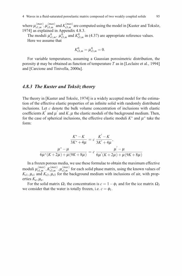
4 Waves in a fluid-saturated poroelastic matrix composed of two weakly coupled solids 95
where μ(max)s1,m ,μ(max)
s3,m and K(max)s3,m are computed using the model in [Kuster and Toksoz,¨
as explained in Appendix 4.8.3.The moduli μ0
s1,m, μ0s3,m and K0
s3,m in (4.37) are appropriate reference values.Here we assume that
K0s3,m = μ0
s3,m = 0.
For variable temperatures, assuming a Gaussian porosimetric distribution, theporosity φ may be obtained as function of temperature T as in [Leclaire et al., 1994]and [Carcione and Tinivella, 2000a].
4.8.3 The Kuster and Toksoz theory
The theory in [Kuster and Toksoz, 1974] is a widely accepted model for the estima-tion of the effective elastic properties of an infinite solid with randomly distributedinclusions. Let c denote the bulk volume concentration of inclusions with elasticcoefficients K
′and μ ′
and K,μ the elastic moduli of the background medium. Then,for the case of spherical inclusions, the effective elastic moduli K∗ and μ∗ take theform:
K∗ −K3K∗+4μ
= cK
′ −K
3K ′+4μ
,
μ∗ −μ6μ∗(K+2μ)+μ(9K+8μ)
= cμ ′ −μ
6μ ′(K+2μ)+μ(9K+8μ)
In a frozen porous media, we use these formulae to obtain the maximum effectivemoduli μ(max)
s1,m ,K(max)s3,m ,μ(max)
s3,m for each solid phase matrix, using the known values ofKs1,μs1 and Ks3,μs3 for the background medium with inclusions of air, with prop-erties Ka,μa.
For the solid matrix Ω1 the concentration is c= 1−φ1 and for the ice matrix Ω3
we consider that the water is totally frozen, i.e. c= φ1.
1974]

Chapter 5
Absorbing boundary conditions in elastic andporoelastic media
Abstract In applied geophysics, it is usually needed to simulate the propagationof waves in a bounded region of the subsurface. This requires the use of absorb-ing boundary conditions at the artificial boundaries of the subsurface model so thatspurius reflections be mimimized. This Chapter presents the derivation of this typeof absorbing boundary conditions in elastic and poroelastic media. They will beused later in the Chapters dedicated to simulate wave propagation phenomena.
5.1 The Elastic Isotropic Case
We consider an elastic body Ω and follow the ideas in [Loeve, 1944] and [Santos et al.,
Consider a small disturbance originated in a restricted portion of an elastic solidmedium Ω = Ω1 ∪Ω2 characterized by Lame parameters λ and μ and density ρ .
We may assume that the disturbed portion is bounded at any instant by a surfaceS. If the medium is isotropic and if the disturbance involves dilatation, we mayexpect that the surface S moves normally to itself with velocity
(λ +2μ
ρ)1/2.
If the disturbance involves rotation without dilation, we may expect the velocity ofthe surface to be
(μρ)1/2.
Then, let us assume that the surface moves normally to itself with velocity c and letus seek the conditions that must be satisfied at the moving surface.
Let uc = (uci )1≤i≤3 be the displacement vector. On one side Ω1 of the surface S attime t, the medium is disturbed and uc = 0. On the other side, (Ω2)uc ≡ 0. We takethe velocity c to be directed from the side Ω1 into the side Ω2 so that the disturbance
© Springer International Publishing AG 2016
in Geosystems Mathematics and Computing, DOI 10.1007/978-3-319-48457-0_5
97
1988].
J.E. Santos, P.M. Gauzellino, Numerical Simulation in Applied Geophysics, Lecture Notes

98
Fig. 5.1 Illustration of a smalldisturbance in the domain Ω1and a surface S separating Ω1from the undisturbed regionΩ2.
ν
χ
χ
Ω
2
S
DisturbedRegion
1
2
1
RegionUndisturbed
Ω
O
spreads into parts of the medium Ω2 that were previously undisturbed, see Figure5.1.
Since uc is continuous across S, uc must vanish on S; i.e.,
uc ≡ 0 on S.
Consequently,
∂uci∂x
= ∇uci · χ = 0,
for any χ in the plane defined by
x ·ν = 0,
where ν is the normal to S at the point o and x= (x1,x2,x3).Then it must necessarily be
∇uci = γν , (5.1)
so that∇uci ·ν = γν ·ν = γ;
i.e.,
γ =∂uci∂ν
. (5.2)
Now from (5.1) and (5.2),(∂uci∂x1
,∂uci∂x2
,∂uci∂x3
)=
∂uci∂ν
· (ν1,ν2,ν3).
Thus,
5.1 The Elastic Isotropic Case

5 Absorbing boundary conditions in elastic and poroelastic media 99
Fig. 5.2 Illustration of theprismatic element bounded byS, by the normals to S at theedge of δS, and by a surfaceparallel to S at a distance cδ tfrom it.
ν
δ tc
δ S
∂uci∂ν
=
∂uci∂x1
ν1=
∂uci∂x2
ν2=
∂uci∂x3
ν3. (5.3)
Next, we observe that the equation
uci (x1,x2,x3, t) = 0 on S (5.4)
must be satisfied to the first order in δ t when (x1,x2,x3, t) is substituted by
(x1 + cδ tν1,x2 + cδ tν2,x3 + cδ tν3, t+dt)
in (5.4). Thus,
uci (x1 + cδ tν1,x2 + cδ tν2,x3 + cδ tν3, t+δ t) (5.5)
= uci (x1,x2,x3, t)+∂uci∂x j
ν jcδ t+∂uci∂ t
δ t = 0.
Hence,
∂uci∂ t
+ c∇uci ·ν =∂uci∂ t
+ c∂uci∂ν
= 0 on S. (5.6)
Now from (5.3) and (5.6) we obtain the relations
∂uci∂x jν j
=−1c
∂uci∂ t
, on S, 1 ≤ i≤ 3, j not summed. (5.7)
In (5.7), the derivatives need to be computed from the side Ω1 where there is adisturbance at time t. The dynamical conditions which hold at the surface S arefound by considering the change in momentum of a thin slice of the medium in aneighborhood of S. We mark out a small area δS of S and consider the prismatic

100
element bounded by S, by the normals to S at the edge of δS, and by a surfaceparallel to S at a distance cδ t from it (see Figure 5.2). The volumeVs of the prismaticelement is Vs = cδ t δS.
The equation of momentum is [Loeve, 1944]
ρ uci (x1,x2,x3, t+δ t)cδ t δS=∫ t+δ t
t
∫δSFs,i ≈ δ tFs,iδS, (5.8)
with the traction Fs given by
Fs,i =−σi jν j,
and
σi j(u) = λδi j∇ ·u+2μεi j(u) (5.9)
is the stress tensor of the elastic isotropic solid.The traction Fs acts across the surface S normal direction ν upon the matter on
that side of the surface towards which ν is drawn.Dividing (5.8) by δ t δS and taking limit when δ t → 0 and δS→ 0 we obtain
ρcuci =−σi jν j =− ∂W∂εi j
ν j, 1 ≤ i≤ j. (5.10)
In vector notation (5.10) becomes
ρcuc =−σν =−Fs, on S. (5.11)
Let χ1 and χ2 be two tangent vectors at the point 0 ∈ S. Then from (5.11) we getthe three equations
ρcuc ·ν =−σν ·ν , ρcuc · χ1 =−σν · χ1, ρcuc · χ2 =−σν · χ2. (5.12)
Set
vc1 =1cuc ·ν =
1cuci νi, vc2 =
1cuc · χ1 =
1cuci χ1
i , (5.13)
vc3 =1cuc · χ2 =
1cuci χ2
i vc = (vc1,vc2,v
c3)
t .
In the new variables vci equations (5.12) become
c2ρvc1 =−σν ·ν , c2ρvc2 =−σν · χ1, c2ρvc3 =−σν · χ2. (5.14)
Next we write the right–hand sides of (5.14) in terms of the variables vc1, vc2, and vc3.For that purpose, we first note that using (5.7) we can write εi j(uc) on the surface Sin the form
5.1 The Elastic Isotropic Case

5 Absorbing boundary conditions in elastic and poroelastic media 101
εi j(uc) =12
(∂uci∂x j
+∂ucj∂xi
)=−1
2
(ν j
1cuci +νi
1cucj
). (5.15)
Then, using (5.15) in the constitutive equations (5.9) we get
σi j(uc) = λδi jεii(uc)+2μεi j(uc) (5.16)
= λδi j(− 1
cνiuci
)−μ(
ν j1cuci +νi
1cucj
)(5.17)
=−λvc1δi j−μ(
ν j1cuci +νi
1cucj
). (5.18)
Consequently,
σν ·ν = σi jνiν j =−λvc1δi jνiν j−μ1cuci ν jνiν j−μ
1cucjνiνiν j
=−λvc1 −2μvc1 =−(λ +2μ)vc1, (5.19)
and
σν · χ1 = σi jνiχ1j =−λvc1δi jνiχ1
j −μ1cuci ν jνiχ1
j −μ1cucjνiνiχ1
j
=−μvc2. (5.20)
Similarly,
σν · χ2 =−μvc3. (5.21)
Next note that
εi jνiν j =−12
(1cuci ν j+
1cucjνi)
νiν j
=−12
(1cuci νiν jν j+
1cucjν jνiνi
)=−1
2(vc1 + vc1) =−vc1,
εi jνiχ1j =−1
2
(1cuci ν j+
1cucjνi)
νiχ1j
=−12
(1cuci νiν jχ1
j +1cucjχ1
j νiνi)=−1
2vc2,
and
εi jνiχ2j =−1
2vc3.

102
Let us compute the strain energy density W (εi j) on the surface S in terms of thevariables (vci )1≤i≤3. To simplify the calculations, let us assume that we have changedcoordinates so that ν = (1,0,0), χ1 = (0,1,0), and χ2 = (0,0,1). Then, from (5.13)
vc1 =1cuci νi =
1cuc1, vc2 =
1cuci χ1
i =1cuc2, vc3 =
1cuci χ2
i =1cuc3.
Also, from (5.15) and (5.18),
ε11 =−12
(ν1
1cuc1 +ν1
1cuc1
)=−vc1,
ε12 =−12
(ν2
1cuc1 +ν1
1cuc2
)=−1
2vc2,
ε13 =−12
(ν3
1cuc1 +ν1
1cuc3
)=−1
2vc3,
ε23 =−12
(ν3
1cuc2 +ν2
1cuc3
)= 0,
ε22 = ε33 = 0,
σ11 = λε11 +2με11 =−(λ +2μ)vc1,
σ12 = 2με12 =−2μ12vc2 =−μvc2,
σ13 = 2με13 =−μvc3,σ23 = σ22 = σ33 = 0.
Hence,
2W |S = (σ11ε11 +2σ12ε12 +2σ13ε13) |S ≡ 2Π(vc)
= (λ +2μ)(vc1)2 +2μ(vc2)
2 +2μ(vc3)2.
Thus, if vc = (vc1,vc2,v
c3),
Π(vc) =12(vc)tE vc,
where
E =
⎛⎝λ +2μ 0 00 μ 00 0 μ
⎞⎠Since
∂Π∂vc1
= (λ +2μ)vc1,∂Π∂vc2
= μvc2,∂Π∂vc3
= μvc3,
from (5.19), (5.20) and (5.21), we see that (5.12) can also be written in the form
5.1 The Elastic Isotropic Case
.

5 Absorbing boundary conditions in elastic and poroelastic media 103
ρc2vc1 =−∂Π∂vc1
, ρc2vc2 =−∂Π∂vc2
, ρc2vc3 =−∂Π∂vc3
. (5.22)
In vector form (5.22) is
c2ρvc =∂Π∂vc
=−Fs = E vc. (5.23)
Next write (5.23) in the form
c2ρ1/2vc = ρ−1/2E ρ−1/2ρ1/2vc.
Set
vc = ρ1/2vc,
S = ρ−1/2E ρ−1/2.
Thus, (5.23) can be written in the form
c2vc = S vc. (5.24)
Also, in terms of vc, the strain energy density on the surface S can be written in theform
Π(vc) = Π(vc) =12(vc)tS vc (5.25)
=12[ρ1/2(vc)t ]ρ−1/2
S ρ−1/2(ρ1/2vc) =12vcS vc. (5.26)
Let (ci)1≤i≤3 be the three positive wave speeds satisfying (5.24); i.e., solutions of
det(S − c2I) = 0.
They are equal to
c1 =
√λ +2μ
ρ, c2 = c3 =
√μρ,
corresponding to the compressional and shear modes of propagation, respectively.Let Ni, 1 ≤ i ≤ 3, be the set of orthonormal eigenvectors corresponding to (ci)2,1 ≤ i≤ 3, and let N be the matrix containing the eigenvectors Ni of S as rows andΛ the diagonal matrix containing the eigenvalues (ci)2, 1 ≤ i≤ 3, of S , i.e.,
Λ =
⎛⎝ c21 0 0
0 c22 0
0 0 c23
⎞⎠so that

104
S = NtΛN. (5.27)
Next, let z = (u · ν , u · χ1, u · χ2)t be a velocity vector on the surface S due tothe simultaneous normal arrival of waves of velocities (ci)1≤i≤3. Since the Ni’s areorthonormal, we can write
z= ρ1/2z=3
∑i=1
[Ni,ρ1/2z]eNi.
Set
zci = ρ1/2zci =1ci[Ni,ρ1/2z]eNi, (5.28)
where [·, ·]e denotes the Euclidean inner product. Then zci satisfies the equation (cf.(5.24))
S zci = c2i z
ci , (5.29)
and the strain energy associated with zci satisfies the relation (cf. (5.26))
Π(zci) =12(zci)t S zci .
Now using (5.23) and (5.26) we see that the force Fi on S associated with zci satis-fies the relation
ρ1/2 ∂Π∂zci
= ρ1/2S zci = ρ1/2ρ−1/2
E ρ−1/2ρ1/2zci = E zci =−F(i).
Next we use that the total force Fs on the surface S is equal to the sum of the forcesFi (see argument leading to the proof of this statement in (5.40)); i.e.,
Fs =3
∑i=1
F(i) =−
3
∑i=1
ρ1/2S zci . (5.30)
On the other hand, we can also write
ρ−1/2Fs =
3
∑i=1
[Ni,ρ−1/2Fs]eNi. (5.31)
Consequently, since S zci = c2i z
ci is a vector in the direction of Ni, from (5.30)and (5.31) we have that
S zci =−[Ni,ρ−1/2Fs]eNi, 1 ≤ i≤ 3. (5.32)
Now from (5.28),
5.1 The Elastic Isotropic Case
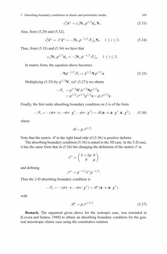
5 Absorbing boundary conditions in elastic and poroelastic media 105
c2i z
ci = ci [Ni,ρ1/2z]eNi. (5.33)
Also, from (5.29) and (5.32),
c2i z
ci = S zci =−[Ni,ρ−1/2Fs]eNi, 1 ≤ i≤ 3. (5.34)
Thus, from (5.33) and (5.34) we have that
ci [Ni,ρ1/2z]e =−[Ni,ρ−1/2Fs]e, 1 ≤ i≤ 3.
In matrix form, the equation above becomes
−Nρ−1/2Fs = Λ 1/2Nρ1/2 z. (5.35)
Multiplying (5.35) by ρ1/2Nt , (cf. (5.27)) we obtain
−Fs = ρ1/2NtΛ 1/2Nρ1/2z,
= ρ1/2S
1/2ρ1/2z= ρS1/2z.
Finally, the first order absorbing boundary condition on S is of the form
−Fs =−(σν ·ν ,−σν · χ1,−σν · χ2) = B(u ·ν , u ·χ1, u ·χ2), (5.36)
where
B = ρS1/2.
Note that the matrix B in the right hand side of (5.36) is positive definite.The absorbing boundary condition (5.36) is stated in the 3D case. In the 2-D case,
it has the same form that in (5.36) but changing the definition of the matrix E to
E∗ =(
λ +2μ 00 μ
)and defining
S∗ = ρ−1/2
E∗ρ−1/2.
Thus the 2-D absorbing boundary condition is
−Fs =−(σν ·ν ,−σν · χ1) = B∗(u ·ν , u ·χ1),
with
B∗ = ρS
∗1/2. (5.37)
Remark. The argument given above for the isotropic case, was extended in[Lovera and Santos, 1988] to obtain an absorbing boundary condition for the gen-eral anisotropic elastic case using the constitutive relation

106
x = 1x
Γ
11
σ
σ
1
1
12
(5.38)
Remark. Let us for simplicity in the argument analyze the 2-D case and theinterface x1 = 1. The work done at any interface averaged over a period is given by(see Figure 5.3)
F =ω2π
∫ 2πω
0(σ11u1 +σ12u2)dt.
F represents the energy flux across the interface and since σi j and u j are con-tinuous, we have conservation of energy. Since
ε11 =1cu1 =−vc1, ε12 =−1
21cu2 =−1
2vc2
we may rewrite F in the form
F =−1c
ω2π
∫ 2πω
0(σ11ε11 +2σ12ε12)dt =−1
cω2π
∫ 2πω
0Π(vc)dt.
For a wavefront arriving to Γ we may decompose the displacement ui in the form
ui = ui,p+ui,s
associated with the compressional and shear modes of propagation.Then we can define the partial fluxes as:
Fk,k =ω2π
∫ 2πω
0(σ11,ku1,k+σ12,ku2,k)dt, k = p,s,
F j,k =ω2π
∫ 2πω
0(σ11, ju1,k+σ12, ju2,k)dt, j,k = p,s, j = k,
5.1 The Elastic Isotropic Case
Fig. 5.3 Illustration of thework done on the Surface Γ
σi j =Ci jklεkl
.
.

5 Absorbing boundary conditions in elastic and poroelastic media 107
where σi j,p denotes the stress associated with the compressional mode and likewisefor σi j,s. It can be seen that F j,k = 0 for j = k ([Dutta and Ode, 1983]). This showsthat the energy flux on Γ can be written as the sum of the energy fluxes associatedwith each type of wave, so that
Π(z) =3
∑i=1
Π(zci), Π(z) =3
∑i=1
Π(zci). (5.39)
Thus, the force on Γ can be written as
−Fs =3
∑i=1
∂Π∂zci
=−3
∑i=1
F(i). (5.40)
5.2 The case of a porous elastic solid saturated by a single-phasefluid
Let us consider the case of an isotropic fluid–saturated porous solid Ω = Ω1 ∪Ω2
where a small disturbance has originated on one side Ω1 of the surface S, which isthe boundary between the disturbed region Ω1 and the undisturbed region Ω2. Thewave front is arriving normally to S with velocity c. Following the ideas leading to(5.11), we see that the conservation of momentum on S can be written as
cA
(us,c
u f ,c
)= (−τi jν j, p f νi) =
(− ∂W
∂εi jν j,
∂W
∂ξνi), 1 ≤ i≤ 3, (5.41)
where
A =
⎛⎝ ρI ρ f I
ρ f I gI
⎞⎠ ,
and I denotes the identity matrix in R3×3. Equation (5.41) can also be written in theform
c(ρ us,c+ρ f u f ,c) =−τi jν j =−∂W
∂εi jν j, on S, (5.42)
c(ρ f us,c+gu f ,c) = p f νi =∂W
∂ξνi, on S. (5.43)
As in the elastic case, let χ1 and χ2 be two tangent vectors at the point o ∈ S (seeFigure 5.1). Taking the inner product with χ1 and χ2 in (5.43) we see that
c(ρ f us,c · χk+gu f ,c · χk) = 0, k = 1,2,

108
so that
u f ,c · χk =−g−1ρ f us,c · χk, k = 1,2. (5.44)
Hence, taking the inner product with ν and χ1, χ2 in (5.42) and using (5.44) weobtain the equations
c[ρ us,c ·ν +ρ f u f ,c ·ν ] =−τν ·ν , (5.45)
c[ρ us,c · χk−g−1ρ f us,c · χk] =−τν · χk, k = 1,2. (5.46)
Also, taking the inner product with ν in (5.43) we obtain
c[ρ f us,cν +gu f ,c ·ν ] = p f . (5.47)
Set vc = (vc1,vc2,v
c3,v
c4)
t , where
vc1 =1cus,c ·ν , vc2 =
1cus,c · χ1,
vc3 =1cus,c · χ2, vc4 =
1cu f ,c ·ν .
Then in the new variables vci equations (5.45), (5.46) and (5.47) become
c2[ρv1 +ρ f v4] =−τν ·ν , c2qv2 =−τν · χ1, (5.48)
c2qv3 =−τν · χ2, c2[ρ f v1 +gv4] = p f , on S,
whereq= ρ −g−1(ρ f )
2.
Next we use the constitutive equations (cf.(1.16)-(1.17)),
τi j = (λues−Bξ )δi j+2μεi j(us), p f =−Bes+Mξ
with
es = ∇ ·us, ξ =−∇ ·u f ,
and (5.15) to write the right hand side of (5.48) in terms of the variables (vci )1≤i≤4.First note that
ξ =−∇ ·u f ,c =−εii(u f ,c)
=12
(νi
1cu f ,ci +νi
1cu f ,ci
)= u f ,c ·ν = vc4.
Thus,
τi j = (λu εii(us,c)−Bv4)δi j+2μ εi j(us,c)
5.2 The case of a porous elastic solid saturated by a single-phase fluid

5 Absorbing boundary conditions in elastic and poroelastic media 109
=−(λu vc1 +Bvc4)δi j−μ
(ν j
1cus,ci +νi
1cus,cj
).
Consequently,
τν ·ν = τi jνiν j =−(λu vc1 +Bvc4)δi jνiν j−μ
1cus,ci ν jν jνi
−μ1cus,cj νiνiν j =−(λu+2μ)vc1 −Bvc4,
τν · χ1 = τi jνiχ1j =−(λu v
c1 +Bvc4)δi jνiχ
1j −μ
1cus,ci ν jνiχ1
j
−μ1cu2,cj νiνix1
j =−μ vc2,
τν · χ2 =−μ vc3,
p f = Bvc1 +Mvc4.
Set
F =(τν ·ν ,τν · χ1,τν · χ2,−p f
)t,
Ap =
⎛⎜⎜⎝ρ 0 0 ρ f
0 q 0 00 0 q 0
ρ f 0 0 g
⎞⎟⎟⎠ , Ep =
⎛⎜⎜⎝λu+2μ 0 0 B
0 μ 0 00 0 μ 0B 0 0 M
⎞⎟⎟⎠ .
Then, in matrix form, equation (5.48) becomes
c2Apvc = Epvc =−F . (5.49)
Next, a calculation similar to that given for the elastic solid case shows that thestrain energy density W (εi j,ξ ) on the surface S can be written in terms of the vari-ables (vci )1≤i≤4 in the form
Π(vc) =12(vc)tEpvc.
Thus, (5.49) can also be stated in the equivalent form
c2Apvc =
∂Π(vc)∂vc
= Epvc =−F , on S. (5.50)
Set
vc = A1/2p vc, (5.51)
S = A−1/2p EpA
−1/2p . (5.52)

110
Then (5.50) becomes
S vc = c2vc. (5.53)
Also, in terms of vc the strain energy density on S can be written in the form
Π(vc) = Π(vc) =12(vc)tEpvc
=12(vc)t(Ap)
1/2(Ap)−1/2
Ep(Ap)−1/2(Ap)
1/2vc =12(vc)tS vc.
Let (ci)1≤i≤4 be the four positive wave speeds satisfying (5.53); i.e., solutions of theequation
det(S − c2I) = 0.
Two of these roots are
c2 = c3 =
(μ
ρ −g−1ρ f
)1/2
,
and they correspond to the shear modes of propagation. The other two roots areassociated with the compressional models of propagation; i.e., the P1 and P2 com-pressional waves.
Next, let Ni, 1 ≤ i ≤ 4, be the set of orthonormal eigenvectors corresponding to(ci)2, 1 ≤ i≤ 4, and let N be the matrix containing the eigenvectors Ni of S as rowsand Λ the diagonal matrix containing the eigenvalues (ci)2, 1 ≤ i≤ 4, of S , i.e.,
Λ =
⎛⎜⎜⎝c2
1 0 0 00 c2
2 0 00 0 c2
3 0B 0 0 c2
4
⎞⎟⎟⎠ (5.54)
so that
S = NtΛN.
Next, let
z= (us ·ν , us · χ1, us · χ2, u f ·ν)t
be a general velocity on the surface S due to the simultaneous arrival of waves ofspeeds (ci), 1 ≤ i≤ 4. Let
z= Ap1/2z.
Then we can write z in the form
5.2 The case of a porous elastic solid saturated by a single-phase fluid

5 Absorbing boundary conditions in elastic and poroelastic media 111
z=4
∑i=1
[Ni,z]eNi =4
∑i=1
[Ni,Ap1/2z]eNi.
Set
zci = Ap1/2zci ≡ 1
ci[Ni,Ap
1/2z]eNi, 1 ≤ i≤ 4. (5.55)
Since zci is a multiple of Ni, we see that
S zci = c2i z
ci , (5.56)
and
Π(zci) =12(zci)tS zci .
Also, using (5.50) we see that the force Fi on S associated with zci satisfies theequation
Ap1/2 ∂Π
∂zci= Ap
1/2S zci = Ap
1/2Ap
−1/2EpAp
−1/2Ap
1/2zci (5.57)
= Epzci =−F(i).
It is known that the interaction among the different types of waves arriving atan interface in a saturated porous medium is small compared with the total energyinvolved ([Dutta and Ode, 1983, Santos et al., 1992]). Neglecting such interactions,we can write the total strain energy density on S as the sum of the partial energies;i.e.,
Π(z) =4
∑i=1
Π(zci),
and the total force F on the surface S as the sum of forces associated with each zci
so that, according to (5.57),
F =4
∑i=1
F(i) =−
4
∑i=1
Ap1/2
S zci .
On the other hand,
Ap−1/2
F =4
∑i=1
[Ni,Ap−1/2
F ]eNi.
Consequently,
S zci =−[Ni,Ap−1/2
F ]eNi, 1 ≤ i≤ 4. (5.58)

112
Now using (5.55), (5.56), and (5.58), we see that
c2i z
ci = S zci = c2i
1ci[Ni,A
1/2p z]eNi =−[Ni,A
−1/2p F ]eNi, 1 ≤ i≤ 4.
Thus,
ci[Ni,A1/2p z] =−[Ni,Ap
−1/2F ]e, 1 ≤ i≤ 4.
In matrix form, the equation above becomes
−NA−1/2p F = Λ 1/2NAp
1/2z. (5.59)
Hence, multiplying (5.59) by Ap1/2Nt = (NAp
1/2)t , we obtain
−(τν ·ν ,τν · χ1,τν · χ2,−p f)= Bp(us ·ν , us · χ1, us · χ2, u f ·ν)t , (5.60)
where
Bp = [NAp1/2]tΛ 1/2[NA
1/2p ] = Ap
1/2S
1/2Ap
1/2 =[(
Ap−1
Ep)t]1/2
(5.61)
Equation (5.60) defines the first–order absorbing boundary conditions on the surfaceS, with the matrix S defined in (5.52).
Note that NAp1/2 is nonsingular and, consequently, Bp in (5.61) is positive def-
inite.The absorbing boundary condition (5.60) is stated in the 3-D case. For the 2-D
case, it has formally the same form:
−(τν ·ν ,τν · χ1,−p f)= B
∗p(u
s ·ν , us · χ1, u f ·ν)t ,
where
B∗p = [N∗
A∗p
1/2]t(Λ ∗)1/2[N∗A
∗p
1/2], (5.62)
and
A∗p =
⎛⎝ ρ 0 ρ f
0 q 0ρ f 0 g
⎞⎠ , E∗p =
⎛⎝λ +2μ 0 B0 μ 0B 0 M
⎞⎠ , Λ ∗ =
⎛⎝ c21 0 0
0 c22 0
0 0 c23
⎞⎠ .
In (5.62) N∗ is the matrix containing as rows the eigenvectors of the matrix
S∗ = A
∗p−1/2
E∗p A
∗p−1/2.
5.2 The case of a porous elastic solid saturated by a single-phase fluid
Ap.

5 Absorbing boundary conditions in elastic and poroelastic media 113
5.3 The case of an isotropic porous solid saturated by atwo-phase fluid
Here we consider a poroelastic medium Ω with boundary ∂Ω saturated by a two-phase fluid. In the 2-D case let χ be a unit tangent on Γ so that ν ,χ is an or-thonormal system on Γ . In the 3-D case let χ1 and χ2 be two unit tangents on Γ sothat ν ,χ1,χ2 is an orthonormal system on Γ .
The argument to derive an absorbing boundary condition is similar to that givenin Section 5.2, and is omitted. Here we state these boundary conditions using thenotation in Chapter 2.
In the 3-D case, the absorbing boundary condition is(τ(u)ν ·ν ,τ(u)ν · χ1,τ(u)ν · χ2,Tn,Tw
)= iωBp
(us ·ν ,us · χ1,us · χ2,un ·ν ,uw ·ν) ,
where
Bp = [(A
−1p Ep
)t]
12 Ap = A
12p S
12 A
12p
with
S = A− 1
2p EpA
− 12
p ,
Ap =
⎛⎜⎜⎜⎜⎝ρ 0 0 Snρn Swρw
0 ρ 0 0 00 0 ρ 0 0
Snρn 0 0 gn gnwSwρw 0 0 gnw gw
⎞⎟⎟⎟⎟⎠ , Ep =
⎛⎜⎜⎜⎜⎝λu+2μ 0 0 B1 B2
0 μ 0 0 00 0 μ 0 0B1 0 0 M1 M3
B2 0 0 M3 M2
⎞⎟⎟⎟⎟⎠ .
In the 2-D case the absorbing boundary condition is(τ(u)ν ·ν ,τ(u)ν · χ1,Tn,Tw
)= iωB
∗p
(us ·ν ,us · χ1,un ·ν ,uw ·ν)
where
B∗p = [(A
∗p−1
E∗p
)t]
12 A
∗p = A
∗p
12 S
∗ 12 A
∗p
12
withS
∗ = Ap− 1
2 E∗p A
∗p− 1
2 ,
and
A∗p =
⎡⎢⎢⎣ρ 0 Snρn Swρw
0 ρ 0 0Snρn 0 gn gnwSwρw 0 gnw gw
⎤⎥⎥⎦ , E∗p =
⎡⎢⎢⎣λu+2μ 0 B1 B2
0 μ 0 0B1 0 M1 M3
B2 0 M3 M2
⎤⎥⎥⎦ .

114
5.4 The case of a composite solid matrix saturated by asingle-phase fluid
Let us consider a fluid-saturated poroelastic material Ω which matrix is composedof two weakly coupled solids; the fluid is assumed to be single-phase. Here we usethe notation in Chapter 4.
Assume that a wave front is arriving at a surface S with velocity c> 0. Denote byu(i,c), i= 1,2,3, the displacements in the i-phase in Ω associated with a wave frontsarriving normally to any part of S with speed c.
Ignoring dissipative effects the conservation of momentum on Γ can be writtenas
cA(u(1,c), w(c), u(3,c)
)t= (−σ (1,T )
i j ν j, p f νi,−σ (3,T )i j ν j)
t
=
(− ∂W
∂εi j(u1,c)ν j,
∂W
∂ζνi,− ∂W
∂εi j(u3,c)ν j
), 1 ≤ i≤ 3. (5.63)
Note that (5.63) is equivalent to the three equations
c
(m11u
(1,c) +m12w(c) +m13u
(3,c))=−σ (1,T )ν , (5.64)
c
(m12u
(1,c) +m22w(c) +m23u
(3,c))= p f ν , (5.65)
c
(m13u
(1,c) +m23w(c) +m33u
(3,c))=−σ (3,T )ν . (5.66)
Let χ1,χ2 be two unit tangent vectors of S so that ν ,χ1,χ2 form an orthonormalset on S. Taking inner product with χ1,χ2 in (5.65) we obtain
w(c) · χk =−m12u(1,c) · χk+m23 ·u(3,c) · χk
m22, ,k = 1,2. (5.67)
Let us introduce the variables
vc1 =1cu(1,c) ·ν , ,vc2 =
1cu(1,c) · χ1, vc3 =
1cu(1,c) · χ2,
vc4 =1cw(c) ·ν vc5 =
1cu(3,c) ·ν , ,vc6 =
1cu(3,c) · χ1, vc7 =
1cu(3,c) · χ2.
Then taking inner product with ν ,χ1,χ2 in (5.64)-(5.66) and using (5.67) we getthat the following seven equations must hold on S:
c2(m11v
c1 +m12v
c4 +m13v
c5
)=−σ (1,T )ν ·ν , (5.68)
5.4 The case of a composite solid matrix saturated by a single-phase fluid

5 Absorbing boundary conditions in elastic and poroelastic media 115
c2(q1v
c2 +q2v
c6
)=−σ (1,T )ν · χ1
c2(q1v
c3 +q2v
c7
)=−σ (1,T )ν · χ2
c2(m12v
c1 +m22v
c4 +m23v
c5
)= p f ,
c2(m13v
c1 +m23v
c4 +m33v
c5
)=−σ (3,T )ν ·ν ,
c2(q2v
c2 +q3v
c6
)=−σ (3,T )ν · χ1,
c2(q2v
c3 +q3v
c7
)=−σ (3,T )ν · χ2,
where
q1 = m11 − m212
m22, q2 = m13 − m12m23
m22, q3 = m33 − m2
23
m22.
Next we write the force
F =
(σ (1,T )ν ·ν ,σ (1,T )ν · χ1,σ (1,T )ν · χ2,−p f ,
σ (3,T )ν ·ν ,σ (3,T )ν · χ1,σ (3,T )ν · χ2)t
on S associated with the arrival of the wave front travelling with speed c in terms ofthe new variable vc = (vci ). For that purpose, note that on the surface S, the straintensor εi j(u(m,c)) and the deviatoric tensor di j(u(m,c)) can be written in the form
εi j(u(m,c)) =12
(∂u(m,c)i
∂x j+
∂u(m,c)j
∂xi
)=−1
2
(ν j
1cu(m,c)i +νi
1cu(m,c)j
), (5.69)
di j(u(m,c)) = εi j(u(m,c))− 13
εll(u(m,c))δi j
=−12
(ν j
1cu(m,c)i +νi
1cu(m,c)j
)+
13
1cu(m,c)l νlδi j ,m= 1,2,3.
Using (5.69) in the constitutive relations
σ (1,T )i j = σ (1)
i j −S1φ p f δi j (5.70)
=[E1θ1 −B1ζ +B3θ3
]δi j+2μ1d
(1)i j +μ1,3d
(3)i j ),
σ (3,T )i j = σ (3)
i j −S3φ p f δi j
,
,

116
=[E3θ3 −B2ζ +B3θ1
]δi j+2μ3d
(3)i j +μ1,3d
(1)i j , (5.71)
p f =−B1θ1 −B2θ3 +Mζ , (5.72)
and defining the matrices
Ap =
⎡⎢⎢⎢⎢⎢⎢⎢⎢⎣
m11 0 0 m12 m13 0 00 q1 0 0 0 q2 00 0 q1 0 0 0 q2
m12 0 0 m22 m33 0 0m13 0 0 m23 m33 0 0
0 q2 0 0 0 q3 00 0 q2 0 0 0 q3
⎤⎥⎥⎥⎥⎥⎥⎥⎥⎦,
Ep =
⎡⎢⎢⎢⎢⎢⎢⎢⎢⎣
E1 +43 μ1 0 0 B1 B3 +
23 μ13 0 0
0 μ1 0 0 0 12 μ13 0
0 0 μ1 0 0 0 12 μ13
B1 0 0 M B2 0 0B3 +
23 μ13 0 0 B2 E3 +
43 μ3 0 0
0 12 μ13 0 0 0 μ3 0
0 0 12 μ13 0 0 0 μ3
⎤⎥⎥⎥⎥⎥⎥⎥⎥⎦,
we conclude that, with vc =(vc1,v
c2,v
c3,v
c4,v
c5,v
c6,v
c7
)t , equations (5.68) can be statedas follows
c2Apvc =−F = Epvc. (5.73)
On the other hand, using (5.69) in (5.70)–(5.72) we conclude that the strain en-ergy density on Π on S can be written in the form
Π(vc) =12(vc)t Ep vc,
so that (5.73) can be stated in the equivalent form
c2Apvc =−F =
∂Π(vc)∂vc
. (5.74)
Set
S = A− 1
2p EpA
− 12
p ,
vc = A12p vc.
In terms of the variable vc (5.73) becomes
5.4 The case of a composite solid matrix saturated by a single-phase fluid

5 Absorbing boundary conditions in elastic and poroelastic media 117
S vc = c2vc,
and the strain energy density Π on S can be written as follows:
Π(vc) =12(vc)t S vc. (5.75)
The seven eigenvalues (ci)2, i= 1, · · · ,7 in the equation
det(S − c2I) = 0
are the squares of the wave speeds of the system. Four of them (only two are dif-ferent) correspond to the shear modes of propagation, and the other three to thecompressional modes.
Let Ni, i = 1, · · · ,7 be the set of orthonormal eigenvectors associated with theeigenvalues (ci)2, i= 1, · · · ,7, and let N be the matrix containing as rows the eigen-vectors Ni and let
Λ = diag(c21, · · · ,c2
7)
be the diagonal matrix containing the eigenvalues (ci)2. Thus,
S = NtΛN.
Let
z=(u(1) ·ν , u(1) ·χ1, u(1) · χ2, w ·ν ,
u(3) ·ν , u(3) · χ1, u(3) · χ2)t
be a general velocity field on Γ due to the simultaneous arrival of waves with speedsci, i= 1, · · · ,7.
Set
z= A12p z
and let us represent z in the form
z= ∑i[Ni,z]eNi = ∑
i[Ni,A
12p z]eNi.
Set
zci = A12p zci =
1ci[Ni,A
12p z]eNi. (5.76)
Since zci is an eigenvector of associated eigenvalue c2i ,

118
S zci = c2i z
ci , (5.77)
and
Π(zci) =12(zci)t S zci .
Also, using (5.74) and (5.75), we see that the force Fi associated with zci satisfiesthe equation
A12p
∂Π(zci)∂zci
= A12p S zci = Epzci =−Fi.
Assuming that the interaction among the different waves arriving at a given in-terface Γ is small compared with the total energy involved (see [Santos et al., 1988]for the validity of this assumption in the case of a single solid phase), the total strainenergy density on S is equal to the sum of the partial energies and the total force F
on S is equal to the sum of the forces associated with each type of wave, so that
Π(z) = ∑i
Π(zci),
and
F = ∑i
Fi = (5.78)
Next, decomposing in term of the eigenvectors Ni,
A− 1
2p F = ∑
i[Ni,A
− 12
p F ]eNi. (5.79)
Next, using (5.76)-(5.77) in (5.78) we see that
=−∑i
S zci =−∑ic2i z
ci =−∑ci[Ni,A12p z]eNi. (5.80)
Thus, from (5.79) and (5.80) we conclude that
=−[Ni,A− 1
2p F ]e. (5.81)
In matrix form, (5.81) becomes
Λ12 NA
12p z=−NA
− 12
p F ,
and multiplying (5.81) to the left by (NA12p )t we see that under the assumption of
small interaction among the different types arriving simultaneously to S, the absorb-ing boundary condition on S can be stated in the form
5.4 The case of a composite solid matrix saturated by a single-phase fluid
A− 1
2p F
A− 1
2p F
−∑i
A12 S zci .p
ci[Ni,A12 z]ep

5 Absorbing boundary conditions in elastic and poroelastic media 119
−F = Bpz (5.82)
where
Bp = A12p S
12 A
12p =
(EpA
−1p
) 12
Ap. (5.83)
Note that Bp is positive definite.The absorbing boundary condition (5.82) was formulated in the 3-D case.In the 2-D case the absorbing boundary condition has the same formal form, with
the matrix B defined as in (5.83) but changing the definitions of the matrices A andE by removing their third and seventh rows and columns. Also, F and z in (5.82)must be redefined removing their third and seventh components.
Chapter 6
Solution of differential equations using the finiteelement method
Abstract The finite element method (FEM) is a useful tool to solve boundary valueproblems of interest in applied geophysics. 1-D finite element spaces are first de-fined and analyzed. The concept of continuous and discrete weak solutions is in-troduced and a priori error estimates are stated. The FEM is used to solve wavepropagation problems and to characterize fine layered media in the 1-D case. Next,2-D and 3-D conforming and non-conforming finite element spaces and definedover partitions of a bounded domain into triangular or rectangular elements in 2-Dand tetrahedral or 3-rectangular elements in 3-D. These finite element spaces areused in the following Chapters to represent solid or fluid vector displacements inthe boundary value problems to be formulated and solved using the FEM.
6.1 Introduction
This Chapter presents the use of the finite element technique to find approximatesolutions to boundary problems appearing in applied geophysics.
The basic idea of the finite element method is to use a partition the domain into aset of sub-domains, the finite element partition, where the solution is being sought,and using what is known as the weak formulation of the original problem to deter-mine an approximate solution over such partition.
To illustrate the finite element approach to solve boundary value problems twosimple model problem are considered. The first is the propagation of waves in one-dimensional viscoelastic media with absorbing boundary conditions. These bound-ary conditions act to make the boundaries transparent for arriving waves, thus al-lowing to simulate wave propagation in unbounded domains.
The second model problem consists of simulating the seismic response of a peri-odic sequence of fine viscoelastic layers. Many geological systems can be modeledas effective transversely isotropic and viscoelastic (TIV) media. Fine layering is a
© Springer International Publishing AG 2016
in Geosystems Mathematics and Computing, DOI 10.1007/978-3-319-48457-0_6
121J.E. Santos, P.M. Gauzellino, Numerical Simulation in Applied Geophysics, Lecture Notes

122
typical example which refers to the case when the dominant wavelength of the trav-elling waves is much larger than the average thicknesses of the single layers.
Backus [Backus, 1962] obtained the average elastic constants in the case whenthe single layers are transversely isotropic and elastic (lossless), with the symmetryaxis perpendicular to the layering plane.
Backus averaging was verified numerically in [Carcione et al., 1991], and gener-alized to the anelastic case in [Carcione, 1992] in what constitutes the Backus/Carcione(BC) theory to describe anisotropic attenuation [Carcione, 2014].
In the second model problem we perform 1-D time-harmonic finite element ex-periments to determine the effective stiffness coefficient for waves travelling nor-mally to the periodic layering. The numerical results are validated against the BCtheory.
Next, a set of finite element spaces to be used in the following chapters to solveboundary value problems in 2-D and 3-D are defined and analyzed.
6.2 The differential model problem for 1-D wave propagation
The 1-D wave propagation problem in viscoelastic media is one of the simplest ex-amples we can develop since it is represented by a second order differential equationwith boundary conditions at the two endpoints of the domain. For this purpose, letu= u(x) denote the displacement of the viscoelastic medium and let
ε(u) =∂u∂x
(6.1)
be the strain tensor.Then, with σ(u) denoting the stress tensor and ω the angular frequency, the
stress-strain relations, stated in the space-frequency domain, are
σ(u) = E(ω)ε(u), (6.2)
where E(ω) = λ (x,ω)+2μ(x,ω) is the complex plane-wave modulus and the co-efficients λ (x,ω) and μ(x,ω) are the complex and frequency dependent Lame co-efficients of the viscoelastic material. Also,
λ (x,ω) = K(x,ω)− 23
μ(x,ω)
with K(x,ω) denoting the bulk modulus. To represent the viscoelastic behaviourof the material, we model the bulk and shear moduli using their relaxed (zero fre-quency) values Kr and μr and the models described in Appendix 1.9.
Recall that for either the Zener or the Liu models of viscoelasticity, we have that,for any ω > 0,
E(ω) = ER(ω)+ iEI(ω), ER(ω)> 0, EI(ω)> 0,
6.2 The differential model problem for 1-D wave propagation
123
limω→0
E(ω) = E(r),
limω→∞
E(ω) = E(u),
with ER(ω) and EI(ω) denoting the real and imaginary parts of E(ω) and E(r),E(u) the relaxed and unrelaxed values of E(ω). Space and frequency are the naturalcoordinates to express the equation of motion.
Next let us consider a domain Ω = (0,L) with boundary ∂Ω = 0,L; we for-mulate the following boundary value problem in the space-frequency domain asfollows: find u(x,ω) such that
−ω2ρ(x)u(x,ω)−∇ ·σ(u(x,ω)) = f (x,ω), x ∈ Ω , ω ∈ R, (6.3)
−σ(u(x,ω)ν = B(x,ω)u(x,ω), x ∈ ∂Ω , ω ∈ R, (6.4)
where ρ = ρ(x) denotes the mass density and (6.4) is an absorbing boundary con-dition. Also, f (x,ω) is the time Fourier transform of an external real valued sourcef(x,t) to be used to excite the medium and generate travelling waves. It will be as-sumed that
f (x, t) = 0, t ≤ 0.
Note that since the solution u(x, t) is real, the
u(x,−ω) = u(x,ω)
and consequently only the case ω > 0 needs to be considered. Here u denotes thecomplex conjugate of u.
In this model problem we intend to simulate the propagation of waves in anunbounded domain. In the boundary condition (6.4) the coefficient B(ω) is usedhere for this purpose, which acts eliminating spurious reflections from the artificialboundaries. It has the form:
B(ω) = iωα −ωβ ,
α = ρA
(A)2 +(B)2β = ρ
B
(A)2 +(B)2,
A=
√√√√12
(c2R
c4R+ c4
I+
√c4R− c4
I
c4R+ c4
I
),
B=1
2A
cIc2R+ c2
I,
cR =
√ER
ρ, cI =
√EI
ρ.
6 Solution of differential equations using the finite element method

124
In many cases of practical interest, the coefficients λ and μ are discontinuous,such as piecewise constants, and the external source may not even be a function, butinstead Dirac distributions or derivatives in the space variable of Dirac distributions,modeling the spatial location of point sources.
Consequently, the solution of (6.3)-(6.4) may not exist in the classical sense, i.e.,asking that the solution be smooth and that such equations be valid at every point.
Thus, we formulate the problem in a weak form, in order to be able to solve prob-lems not satisfying strong smooth requirements on their coefficients or the externalsources.
6.3 A variational formulation for the 1-D wave propagationmodel problem
To overcome the above mentioned difficulties, we shall reformulate the boundary-value problem in a way that will admit weaker conditions on the solution and itsderivatives. Such reformulations are called weak or variational formulations of theproblem and are designed to accommodate irregular data and irregular solutions.
As stated in Section 6.2, instead of asking the validity of (6.3) point-wise, wereformulate the problem and we will require its validity with weaker conditions onthe solution and its derivatives. In this sense, we write the variational or weak formof the problem requiring that the equation
−ω2∫
Ωρu(x,ω)v(x)dx−
∫Ω
∇ ·σ(u(x,ω))v(x)dx
=∫
Ωf (x,ω)v(x)dx (6.5)
be valid for test functions v belonging to a set to be specified later. Here v denotesthe complex conjugate of the function v. Also, we use ∇ · σ(u(x,ω)) to denote∂σ(u(x,ω))
∂x.
Using integration by parts in the second term in the left-hand side of (6.5) weobtain
−ω2∫
Ωρu(x,ω)v(x)dx+
∫Ω
σ(u(x,ω))ε(v(x))dx−∫
∂Ωσ(u(x)) ·ν v(x)d(∂Ω)
=∫
Ωf (x,ω)v(x)dx. (6.6)
Thus, applying the boundary condition (6.4) in (6.6) and the definitions of σ(u)and ε(v) in (6.2) and (6.1) we get the equation
6.3 A variational formulation for the 1-D wave propagation model problem
The form of the coefficient B(ω) can be obtained considering plane waves andasking that they satisfy (6.3) at ∂Ω (see [Ravazzoli and Santos, 1995] for details).

125
−ω2∫
Ωρu(x,ω)v(x)dx+
∫ΩE(x,ω)
∂u(x,ω)
∂x∂v(x)
∂xdx (6.7)
+∫
∂ΩB(x,ω)u(x,ω)v(x)d(∂Ω)
=−ω2∫
Ωρu(x,ω)v(x)dx+
∫ΩE(x,ω)
∂u(x,ω)
∂x∂v(x)
∂xdx
+∫
∂Ωiωα(x,ω)u(x,ω)v(x)d(∂Ω)−
∫∂Ω
ωβ (x,ω)u(x,ω)v(x)d(∂Ω)
=∫
Ωf (x,ω)v(x)dx.
Recalling Holder’s integral inequality [Kolmogorov and Fomin, 1970]
∫Ωf (x)g(x)dx≤
(∫Ω| f (x)|2dx
)1/2(∫Ω|g(x)|2dx
)1/2
, (6.8)
it is clear that in order that (6.7) holds, we need that the solution u and the testfunction v as well as their first derivatives be square integrable.
Let C denote the set of complex numbers and let us introduce the space L2(Ω)of square integrable complex valued functions as
L2(Ω) = f : Ω → C such that∫
Ω| f (x)|2dx< ∞.
The space of functions L2(Ω) can be provided with a natural inner product andnorm, denoted by (·, ·) and ‖ · ‖0, respectively, defined as follows:
( f ,g) =∫
Ωf (x)g(x)dx, f ,g ∈ L2(Ω),
‖ f‖0 =
(∫Ω| f (x)|2dx
)1/2
, f ∈ L2(Ω).
Besides, we define the space H1(Ω) of functions in L2(Ω) having square integrablefirst derivatives by
H1(Ω) = v ∈ L2(Ω) such that∫
Ω
∣∣∣∣∂v(x)∂x
∣∣∣∣2 dΩ < ∞.
‖v‖1 =
(∫Ω|v(x)|2dx+
∫Ω
∣∣∣∣∂v(x)∂x
∣∣∣∣2 dx)1/2
, v ∈ H1(Ω). (6.9)
The natural norm defined on H1(Ω) is
6 Solution of differential equations using the finite element method
126
Also, it is convenient to define the inner product in ∂Ω = 0,L as
〈 f ,g〉= f (0)g(0)+ f (L)g(L). (6.10)
Using this notation, we can state the original model problem in weak or variationalform as follows: find u ∈ H1(Ω) such that
Λ(u,v) =−ω2 (ρu,v)+(E
∂u∂x
,∂v∂x
)+ 〈iωα u,v〉−
⟨ωβ u,v
⟩(6.11)
= ( f ,v) , ∀ v ∈ H1(Ω).
Note that in the above formulation, the boundary condition (6.4) has been imposedweakly, i.e., it has not been required that the test functions v satisfy (6.4).
The existence of a solution of (6.11) follows from a functional analysis argumentusing the Fredholm alternative [Yosida, 1980]. The proof is outside the scope of thisbook and is omitted.
Let us turn to analyze uniqueness of the solution of problem (6.11). For thatpurpose, we assume there are two solution, u1 and u2, then the difference is u =u1 − u2 and satisfies (6.11) for f = 0. Thus set f = 0 and take v = u in (6.11) toobtain
−ω2 (ρu,u)+((ER+ iEI)
∂u∂x
,∂u∂x
)+ 〈iωα u,u〉−
⟨ωβ u,u
⟩= 0. (6.12)
Taking the imaginary part in (6.12) we obtain(EI
∂u∂x
,∂u∂x
)+ 〈ωα u,u〉= 0. (6.13)
Since EI > 0,α > 0, it follows from (6.13) that
‖∂u(·,ω)
∂x‖0 = 0, u(x,ω) = 0, x ∈ 0,L. (6.14)
Next, from (6.14), assuming that u(x,ω) is smooth, we can write,
u(x,ω) =∫ x
0
∂u(z,ω)
∂ zdz (6.15)
so that squaring the equation in (6.15) and using (6.8) with f = u and g= 1 leads tothe inequality
|u(x,ω)|2 =∣∣∣∣∫ x
0
∂u(z,ω)
∂ zdz
∣∣∣∣2 dz≤ ∫ x
0|∂u(z,ω)
∂ z|2dz∫ L
0dz
≤ L∫ L
0|∂u(z,ω)
∂ z|2dz. (6.16)
6.3 A variational formulation for the 1-D wave propagation model problem

127
Integration of (6.16) in the variable x yields
‖u(·,ω)‖0 ≤ L‖∂u(x,ω)
∂x‖0. (6.17)
Inequality (6.17) is know as Poincare’ s inequality. Consequently
‖u(·,ω)‖0 = 0,
and we have uniqueness for the solution of (6.11) assuming that u(·,ω) is smooth.An argument involving the density of smooth functions in the space H1(Ω)
[Adams, 1975], it can be shown that
∥∥∥∥∂v∂x
∥∥∥∥0
defines a norm ‖| · ‖| equivalent to
the ‖ · ‖1-norm defined in (6.9) in the space of functions
H10 (Ω) = v ∈ H1(Ω) such that v= 0 on 0,L.
Hence, (6.14) says that u(·,ω) ∈ H10 (Ω) and ‖|u(·,ω)‖| = 0, so that uniqueness
holds for the solution of (6.11).Note that the space H1(Ω) where we are seeking the solution of (6.11) is infinite-
dimensional. Thus we would need an infinite number of coefficients to represent thesolution u in any basis of H1(Ω).
Consequently, we will consider the problem of finding an approximate solutionof (6.11) in a appropriate finite dimensional subspace of H1(Ω) using the finiteelement method.
6.4 The finite element procedure
Let T h(Ω) be a non-overlapping partition of Ω into Nx subintervals Ω j =
(x j,x j+1), j = 1, · · · ,Nx, with x j = jh and h =LNx
. In this way, the partition de-
termines a set of finite element, Ω j of length h and in order to complete the finiteelement mesh it is necessary to choose certain points within each element, callednodes or nodal points. In this problem, the nodes are the endpoints of each element.
To approximate the solution u we define the finite element space M h as follows:
Mh = v : v|Ω j ∈ P1(Ω j)∩C0(Ω),
where v|Ω j denotes the values of v restricted to Ω j, P1(Ω j) denotes the polynomials
of degree not greater than 1 in the variable x on Ω j and C0(Ω) are the contin-uous functions in the closed interval Ω = [0,L]. In other words, we will employC0-piecewise linear functions over Ω to seek the approximate solution to problem(6.11).
6 Solution of differential equations using the finite element method

128
wise constant, both v and∂v∂x
are functions in L2(Ω) and consequently M h ⊂H1(Ω).
Thus we are searching for an approximate solution of u in a finite dimensionalspace of piecewise polynomials that is contained in the space H1(Ω) where thesolution u of the continuous problem (6.11) belongs.
When this is the case, it is said that the space M h is a conforming finite elementspace of H1(Ω).
Now the finite element procedure to compute the approximate solution of (6.11)is defined as follows: find uh ∈ M h such that
Λ(uh,v) =−ω2(
ρuh,v)+
(E
∂uh
∂x,
∂v∂x
)+⟨
iωα uh,v⟩−⟨
ωβ uh,v⟩
= ( f ,v) , ∀ v ∈ Mh. (6.18)
Uniqueness for the solution of the (6.18) can be demonstrated with the same argu-ment than for the solution of the continuous problem (6.11). Existence of the solu-tion of (6.18) follows from finite dimensionality (see the argument in the Remarkfollowing (6.23)).
Next, let
uh =Nx+1
∑j=1
u jϕ j. (6.19)
where the function ϕ j, j = 1, · · · ,Nx+1 are defined as
ϕk =
⎧⎪⎪⎪⎪⎪⎪⎨⎪⎪⎪⎪⎪⎪⎩
x− xk−1
hxk−1 ≤ x≤ xk,
1− x− xkh
xk ≤ x≤ xk+1,
0, otherwise.
(6.20)
For k = 1, to define ϕ1, choose in (6.20) the formula corresponding to (x1,x2),and for k = Nx + 1 to define ϕNx+1 select in (6.20) the formula corresponding to(xNx ,xNx+1). Figure 6.1 shows the finite element partition in the domain [0,L] withnodal points, subintervals and piecewise linear functions.
Next we demonstrate that (6.18) is equivalent to solve a tridiagonal system todetermine the coefficients u j in (6.19).
First we show thatM
h = Span ϕ1, · · · ,ϕNx+1.In fact: we have Nx subintervals and on each one we have two parameters defining alinear function, so we have 2 Nx parameters. But on each node x j, j = 1, · · · ,Nx we
6.4 The finite element procedure
Remark. Note that since elements v ∈ M h are continuous in Ω and∂v∂x
are piece-
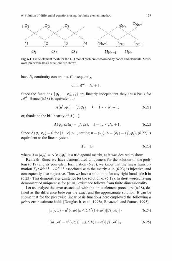
129
ϕϕ
Ω Ω Ω ΩΩΩΩ Ω
1 ϕ
1
1
2
2 3
3 Nx
Nx+1
Nx+1
ϕϕNx
x x x x xx Nx1 2 3
Nx−1
x4 Nx−1Nx−1
Fig. 6.1 Finite element mesh for the 1-D model problem conformed by nodes and elements. More-over, piecewise basis functions are shown.
have Nx continuity constraints. Consequently,
dim Mh = Nx+1.
Since the functions ϕ1, · · · ,ϕNx+1 are linearly independent they are a basis forM h. Hence (6.18) is equivalent to
Λ(uh,ϕk) = ( f ,ϕk) , k = 1, · · · ,Nx+1, (6.21)
or, thanks to the bi-linearity of Λ(·, ·),
Λ(ϕ j,ϕk)u j = ( f ,ϕk), k = 1, · · · ,Nx+1. (6.22)
Since Λ(ϕ j,ϕk) = 0 for | j− k| > 1, setting u = (u j), b = (bk) = ( f ,ϕk), (6.22) isequivalent to the linear system
Au= b, (6.23)
where A= (ak j) = Λ(ϕ j,ϕk) is a tridiagonal matrix, as it was desired to show.
lem (6.18) and its equivalent formulation (6.23), we know that the linear transfor-mation TA : RNx+1 → RNx+1 associated with the matrix A in (6.23) is injective, andconsequently also surjective. Thus we have a solution u for any right-hand side b in(6.23). This demonstrates existence for the solution of (6.18). In short words, havingdemonstrated uniqueness for (6.18), existence follows from finite dimensionality.
Let us analyze the error associated with the finite element procedure (6.18), de-fined as the difference between the exact and the approximate solution. It can beshown that for the piecewise linear basis functions here employed the following apriori error estimate holds [Douglas Jr. et al., 1993a, Ravazzoli and Santos, 1995]:
‖u(·,ω)−uh(·,ω)‖0 ≤Ch2(1+ω2)‖ f (·,ω)‖0 (6.24)
‖(u(·,ω)−uh(·,ω))‖1 ≤Ch(1+ω)‖ f (·,ω)‖0, (6.25)
6 Solution of differential equations using the finite element method
Remark. Since we have demonstrated uniqueness for the solution of the prob-

130
where C is a generic positive constant independent of h depending upon the data ofthe problem and the power of h depends upon the basis functions, being a measure ofthe rate of convergence with respect to the corresponding norm. The error estimatesin (6.24) and (6.25) gives the error bound in terms of powers of the frequency ω andthe mesh size h, giving the exact relation between ω and h needed to reach a desiredaccuracy in the FE calculations. This effect, occurring when solving Helmholtz-type equations, was later denominated pollution by other authors, see for example[Ihlenburg and Babuska, 1997].
It is usual to calculate the error through asymptotic estimates. As the exact solu-tion is in general unknown, the error is measured by its behaviour when h decreasesand the number of elements increases, i.e., when the mesh is refined.
6.5 The algebraic problem associated with the 1-D wavepropagation model problem
To obtain the linear system associated with (6.21) we compute each integral assum-ing that the coefficients ρ and E are piecewise constant. We denote by ρk and Ek tothe values of ρ and E in the subinterval (xk,xk+1).
Since
(ρuh,ϕk) =
(ρ
Nx+1
∑j=1
u jϕ j,ϕk
)=
(ρ
k+1
∑j=k−1
u jϕ j,ϕk
)
and
(ρϕk−1,ϕk) = ρk−1h6(1−δk,1),
(ρϕk,ϕk) = ρk−1h3(1−δk,1)+ρk
h3(1−δk,Nx+1),
(ρϕk+1,ϕk) = ρkh6(1−δk,Nx+1),
we obtain
(ρuh,ϕk) = ρk−1h6(1−δk,1)uk−1 +
[ρk−1
h3(1−δk,1)+ρk
h3(1−δk,Nx+1)
]uk
+ρkh6(1−δk,Nx+1)uk+1. (6.26)
Here δk,1 and δk,Nx+1 denote the Kronecker’s delta, so that the term multipled bythat factor dissapears from the equation when k = 1 or k = Nx+1.
Next, note that
6.5 The algebraic problem associated with the 1-D wave propagation model problem

131(E
∂uh
∂x,
∂ϕk
∂x
)=
(E
k+1
∑j=k−1
u j∂ϕ j
∂x,
∂ϕk
∂x
),
and (E
∂ϕk−1
∂x,
∂ϕk
∂x
)=−1
hEk−1(1−δk,1),(
E∂ϕk
∂x,
∂ϕk
∂x
)=
1hEk−1(1−δk,1)+
1hEk(1−δk,Nx+1),(
E∂ϕk+1
∂x,
∂ϕk
∂x
)=−1
hEk(1−δk,Nx+1).
Thus (E
∂uh
∂x,
∂ϕk
∂x
)=−1
hEk−1(1−δk,1)uk−1 (6.27)
+
[1hEk−1(1−δk,1)+
1hEk(1−δk,Nx+1)
]uk
−1h(1−δk,Nx+1)Ekuk+1.
Next, note that⟨iωαuh,ϕk ·ν
⟩= 0,
⟨ωβuh,ϕk ·ν
⟩= 0 only for k = 1 or k = Nx+1.
Thus using the definition of 〈·, ·〉 in (6.10),⟨iωαuh,ϕk ·ν
⟩−⟨
ωβuh,ϕk ·ν⟩=(
iωαk−ωβk
)ukδk,1 (6.28)
+(
iωαk−ωβk
)ukδk,Nx+1.
Now collecting all terms in (6.26), (6.27) and (6.28) we get the following tridiagonallinear system to be solved for each ω > 0:[
−ω2ρk−1h6− 1
hEk−1
](1−δk,1)uk−1 (6.29)
+
[−ω2
(ρk−1
h3(1−δk,1)+ρk
h3(1−δk,Nx+1)
)+
1hEk−1(1−δk,1)+
1hEk(1−δk,Nx+1)
+(
iωαk−ωβk
)δk,1 +
(iωαk−ωβk
)δk,Nx+1
]uk
+
[−ω2ρk
hk6− 1
hkEk
](1−δk,Nx+1)uk+1
6 Solution of differential equations using the finite element method

132
= ( f ,ϕk), k = 1, · · · ,Nx+1
Equation (6.29) defines the coefficients of the tridiagonal matrix A and the right-hand side vector b in (6.23).
6.6 A numerical example for the 1-D wave propagation problem
In this numerical example the domain Ω is an open interval of size 1000 m. The ma-terial correspond to Nivelsteiner sandstone saturated by a single-phase fluid, wateror gas; with properties indicated in Table 1.1. The interface between the two mediais located at the center of Ω .
The source function is given by the expression
f (x, t) =C∂δ (x)
∂xξ (t− t0)e
−ξ (t−t0)2, t ≥ 0,
where f0=1/t0=50 Hz is the central frequency of the source, ξ = 8 f 20 andC is a con-
stant chosen so that max| f (t)|=1. The Dirac distribution, δ (x), determines the posi-tion of the source, see Figure 6.2 (a) where we also indicate elastic compressionalvelocities for the dry and saturated sandstone and the location of three receivers re-ferred to as R1, R2 and R3. The saturated real plane wave moduli are calculated bythe Gassmann’s approximation (1.15) since frequency range is low: 0-100 Hz.
The mesh has 582 elements which allow to solve with 25 grid points per mini-mum wavelength. The solution is computed at 600 discrete points of the frequencyrange.
For the viscoelastic case we use a continuous distribution of relaxation mech-anisms (see Appendix 1.9) where the values of t1 and t2 are such that the qualityfactor Q is approximately equal to the constant QM in the range t−1
1 ≤ 2π f ≤ t−12 .
In the example we choose QM=148 for the saturated bulk modulus, QM=100 for theshear modulus, t1=10−6 ms and t2=103 ms. Figure 6.2 (b) shows traces of displace-ment in the three receivers. The arrival time of the transmitted waves are designatedby T1, T2 and T3 for receivers 1, 2 and 3, respectively. The arrival time of the re-flected waves at the interface are denoted by R1 and R2. Observe that the absorbingboundary condition eliminates reflections at the boundaries of the domain. The am-plitude decay observed in the traces represents physical attenuation correspondingto phenomena included in the viscoelastic model.
We emphasize that in this algorithm the solution is computed separately for eachfrequency and only a limited number of them are needed to recover correctly thesolution in the domain, therefore the numerical procedure is naturally suited to beused in parallel computers. This property becomes a necessity when dealing withrealistic problems in two or three dimensions.
6.6 A numerical example for the 1-D wave propagation problem

133
R3R2R1*Source
200 m
400 m
950 m
Vpsat=2415 m/s sat=2545 m/sVp
Water saturated sandstone Gas saturated sandstone
Vpdry=1870 m/s
15452415
(a)
0 100 200 300 400 500Time (ms)
-0,05
0
0,05
Receiver 1Receiver 2
Receiver 3
T1 T2 T3
R1R2
(b)
Fig. 6.2 1-D geometrical model (a) and the traces of displacement at the three receivers (b).
6 Solution of differential equations using the finite element method

134
6.7 The model problem to perform harmonic experiments in 1-Dfine layered media. Backus averaging validation
As mentioned in the introduction, many geological systems can be modeled as effec-tive transversely isotropic and viscoelastic media. Fine layering is a typical examplewhich refers to the case when the dominant wavelengths of the travelling waves aremuch larger than the average thickness of the single layers.
Here we determine the complex and frequency dependent coefficient defining a1-D viscoelastic medium equivalent to a finely layered 1-D viscoelastic material.The results are validated against the Backus-Carcione (BC) theory.
The methodology consists in applying time-harmonic oscillatory tests to a 1-D numerical rock sample for a finite number of frequencies. These tests can beregarded as an up-scaling method to carry the effect of the fine layering scale to themacro-scale.
If x3 denote the vertical coordinate, a fine layered viscoelastic medium behavesas a viscoelastic and homogeneous equivalent viscoelastic medium at long wave-lengths.
Let u denote the displacement at the macro-scale and let
e33(u) =∂ u∂x3
the strain tensor at the macro-scale.If σ(u) is the stress tensor of the equivalent 1-D medium at the macro-scale,
the corresponding stress-strain relation, stated in the space-frequency domain, is[Carcione, 1992]
σ33(u) = p33 e33(u),
where
p33 = 〈E−1〉−1 (6.30)
E = λ +2μ is the complex plane wave modulus of each single layer and 〈 · 〉 denotesthe thickness weighted average.
The p33 is the complex and frequency-dependent Voigt stiffnesses to be deter-mined with the harmonic experiments.
6.8 Determination of the stiffness p33
Assume that the medium Ω is composed of a sequence of isotropic linear viscoelas-tic layers Ωn, n= 1, · · · ,N, and on each Ωn the constitutive relations are
6.8 Determination of the stiffness p33
.

135
σ(u) = En(x,ω)ε(u) (6.31)
where En = λn+2μn is the complex plane wave modulus of the n-layer and ε(u) isthe strain tensor on each fine layer.
Then if ρ = ρ(x3) is the mass density, the equation of motion is
−ω2ρu−∇ ·σ(u) = 0, (6.32)
with σ(u) given by (6.31).Set
Γ B = x= 0, Γ T = x= L.Then we solve (6.32) with the following boundary conditions
σ(u)ν ·ν =−ΔP, x ∈ Γ T , (6.33)
u= 0, x ∈ Γ B. (6.34)
For this set of boundary conditions the material is not allowed to move on the bottomboundary Γ B and a uniform compression is applied on the boundary Γ T .
Denoting by V the original volume of the sample, its (complex) oscillatory vol-ume change, ΔV (ω), allows us to define the equivalent complex plane-wave modu-lus p33(ω), by using the relation
ΔV (ω)
V=− ΔP
p33(ω),
valid for a viscoelastic homogeneous medium in the quasi-static case.After solving (6.32) with the boundary conditions (6.33)-(6.34), we can use the
vertical displacements u(L,ω) on Γ T to approximate the volume change producedby the compressibility test:
ΔV (ω)≈ u(L,ω)
which enable us to compute the equivalent complex plane-wave modulus p33(ω) by
p33(ω)≈ −L ΔPu(L,ω)
.
The corresponding complex compressional velocity is
vpc(ω) =
√p33(ω)
ρb,
where ρb is the average bulk density of Ω , given by
ρb =N
∑j=1
fiρi,
6 Solution of differential equations using the finite element method

136
with fi being the volume fraction of the i-layer.The following relations allow us to estimate the equivalent compressional phase
velocity vp(ω) and quality factor Qp(ω) in the form:
vp(ω) =
[Re
(1
vpc(ω)
)]−1
, Qp(ω) =Re(vpc(ω)2)
Im(vpc(ω)2). (6.35)
6.9 A variational formulation for the harmonic experiment infine layered viscoelastic media
Let us introduce the space
H10,B(Ω) = v ∈ H1(Ω) such that v= 0 on Γ B.
Then, proceeding as in the wave propagation model problem, multiply equation(6.32) by a test function v ∈ H1
0,B(Ω), use integration by parts and apply the bound-ary conditions (6.33)- (6.34) to derive the following variational formulation: findu ∈ H1
0,B(Ω) such that
−ω2(
ρuh,v)+
(E
∂uh
∂x,
∂v∂x
)=−〈ΔP,v ·ν〉Γ T , ∀v ∈ H1
0,B(Ω), (6.36)
where E = En on the n-layer.Note that now the boundary condition (6.34) has been imposed on the space of
test functions H10,B(Ω); it is said that this boundary condition (homogeneous Dirich-
let boundary condition) is imposed strongly on space of test functions. On the otherhand, the boundary condition (6.33) was imposed weakly.
Uniqueness for the solution of (6.36) follows with identical argument than for thewave propagation problem (6.11). For a proof of existence of the solution of (6.36)we refer to [Santos et al., 2011].
6.10 The finite element procedure to determine the stiffness p33
Let T h(Ω) be the non-overlapping partition of Ω into Nx subintervals Ω j =(x j,x j+1), j = 1, · · · ,Nx defined in the wave propagation model problem in Section(6.4).
To approximate the displacement vector u we employ the finite element spaceM h
0,B ⊂ H10,B(Ω) defined as follows:
Mh0,B = v : v|Ω j ∈ P1(Ω j), v= 0 on Γ B∩C0(Ω).
6.10 The finite element procedure to determine the stiffness p33

137
As in the previous model problem, M h0,B ⊂ H1(Ω).
Then the finite element procedure to compute the approximate solution of (6.36)is defined as follows: find uh ∈ M h
0,B such that
−ω2(
ρuh,v)+
(E
∂uh
∂x,
∂v∂x
)=−〈ΔP,v ·ν〉Γ T , ∀v ∈ M
h0,B. (6.37)
Uniqueness for the solution uh of (6.37) follows from the same argument than forthe problem (6.18), while existence follows from finite dimensionality.
6.11 The algebraic problem associated to the harmonicexperiment in fine layered viscoelastic media
With the argument given for the wave propagation problem in Section (6.4) it canbe seen that
dimMh0,B = Nx.
Since the functions ϕk, 2,≤ k≤Nx+1 given in (6.20) belong to the space M h0,B and
are linearly independent, they are a basis for the finite element space M h0,B. Hence,
Mh0,B = Spanϕk, 2,≤ k ≤ Nx+1
Next, let us write the finite element function uh ∈ M h0,B as
uh =Nx+1
∑j=2
u jϕ j
and write (6.37) in the equivalent form: find uh ∈ M h0,B such that
−ω2(
ρuh,ϕk
)+
(E
∂uh
∂x,
∂ϕk
∂x
)=−〈ΔP,ϕk ·ν〉Γ T , (6.38)
k = 2, · · · ,Nx+1.
To obtain the linear system associated with (6.38), we proceed as in the wave prop-agation example, computing all integrals in (6.38) assuming piecewise constant co-efficients.
In this fashion, we obtain the following tridiagonal linear system to be solved foreach ω > 0:
[−ω2ρk−1
hk−1
6− 1
hk−1Ek−1
]uk−1
.
6 Solution of differential equations using the finite element method

138
+
[−ω2
(ρk−1
hk−1
3+ρk
hk3(1−δk,Nx+1)
)+
1hk−1
Ek−1 +1hk
Ek(1−δk,Nx+1)
]uk
+
[−ω2ρk
hk6(1−δk,Nx+1)− 1
hk(1−δk,Nx+1)Ek
]uk+1
=−ΔPδk,Nx+1, k = 2, · · · ,Nx+1.
6.12 A numerical example to determine the stiffness p33
The example considers domain Ω of 50 cm size containing 100 alternating subin-tervals of shale and limestone of equal size, so that the spatial period is 1 cm. Weuse Nx = 100 subintervals as finite element mesh, so that h = 0.5 cm.
The properties of the isotropic viscoelastic materials are given in Table 6.1, i.e.,bulk modulusK and shear modulus μ, densities and quality factors [Santos et al., 2011].
Recall that the Lame ’s parameter λ is defined by λ = K− 23
μ , so that the plane
modulus E is determined from the data in Table 6.1 from the relation
E = K+43
μ .
We assume constant quality factors over the frequency range of interest (untilabout 100 Hz), which was modeled by a continuous distribution of relaxation mech-anisms based on the standard linear solid as explained in Appendix 1.9.
Nl(ω) = 1+2
πQMln
1+ iω t21+ iω t1
, l = 1,2. (6.39)
Let the time constants in equation (6.39) be t1 = 0.16 s and t2 = 0.3 ms, so that thequality factor of each single isotropic layer is nearly constant from about 10 Hz to100 Hz.
Table 6.1 Material properties
Medium K (GPa) μ (GPa) ρ (gr/cm3) Q01 Q02
Shale 8.545483 1.7 2.25 60 20
Limestone 63.3354564 25.0 2.7 80 40
plex moduli N1 and N2 for a specific frequency can be expressed asAs already indicated in (1.120), the dimensionless dilatational and shear com-
6.12 A numerical example to determine the stiffness p33

139
Figure 6.3 shows the phase velocity vp(ω) and the plot of 1000/Qp(ω) withvp(ω) and Qp(ω) computed using (6.35). The stiffness p33(ω) was determined us-ing the finite element solution of the harmonic experiments and compared with thecorresponding analytical values of the BC theory in (6.30). A perfect fit can be ob-served.
0 25 50 75 100Frequency (Hz)
3500
3550
3600
3650
3700
3750
3800
Com
pres
sion
al W
ave
Vel
ocity
(m
/s)
AnalyticalNumerical
0 25 50 75 100Frequency (Hz)
10
15
20
25
30
1000
/Qp
AnalyticalNumerical
(a) (b)
Fig. 6.3 Analytical and numerical phase velocity (a) and inverse quality factor (b) for compres-sional waves as function of frequency for the equivalent viscoelastic medium.
6.13 2-D finite element spaces
Here we define some of the finite element spaces that will be used in the next chap-ters to solve problems in two and three dimensions.
6.13.1 Conforming finite element space over triangular partitionsof Ω to represent solid displacements
Let T h be a partition of a bounded domain Ω in the (x,y)-plane into non-overlappingtriangles T i, i = 1, · · · ,N of diameter bounded by h (i.e., h is the diameter of circleinscribed in T i). If in this partition two triangles intersect, the intersection is a com-mon side, so we do not allow a vertex of a triangle be interior to a side of an adjacenttriangle.
If Ω has curved boundary, the partition T h will not cover the original domainΩ , and there will an error associated with this partition of the domain. With small
6 Solution of differential equations using the finite element method

140
enough triangles with vertices touching the boundary, the error will be small for theproblems to be considered here. Thus we consider our domain to be represented as
Ω = ∪Ni=1T
i.
Let us define the first finite element space over the triangulation as follows:
where P1(T i) denotes the polynomials of degree lees or equal to 1 in the variables(x,y).
Note that since functions in M h are continuous and its first derivatives are piece-wise constants we have that M h ⊂ [H1(Ω)]2. Thus M h is a conforming finite ele-ment space of [H1(Ω)]2.
Next we describe a procedure to construct a basis for M h. For any triangle T ofthe partition, if a j = (x j,y j), j = 1,2,3 are the three vertices, to be also referred asnodes of T , the functions ϕ j ∈ P1(T ) have the form
ϕ j(x,y) = p j+q j x+ r j y, j = 1,2,3.
The values of the polynomial ϕ j(x,y) at the three nodes of the triangle T are thelocal degrees of freedom of the finite element. These values uniquely define thepolynomial ϕ j(x,y).
Thus, the equations
ϕk(a j) = δk j, j,k = 1,2,3
define uniquely three linear functions ϕk(x,y),k = 1,2,3 over the triangle T . Theyare a local basis over T .
Then for any given complex (or real) valued function g(x,y) ∈ C0(Ω) we candefine the Lagrange interpolant gI(x,y) constructing a basis φs,s= 1, · · · ,M for M h
using these local bas s.For this purpose, we glue together the local bases
triangles T i and T l having a common side Γ il and a common node ail to constructone basisfreedom. This basis function is such that
φil(ail) = 1,
and φil vanishes at all other nodes of T i and T l . Note that this basis has small sup-port, a very convenient property for computational purposes.
For the case of triangle with a boundary node, we use as global basis only thelocal basis associated with such node.
6.13 2-D finite element spaces
Mh = v= (vx,vy) such that v|T i ∈ [P1(T
i)]2∩ C0(Ω) ,]2
e
[
ϕ ik and ϕ l
s of two adjacent
element φil (x,y)associated with the node ail , which is a global degree of
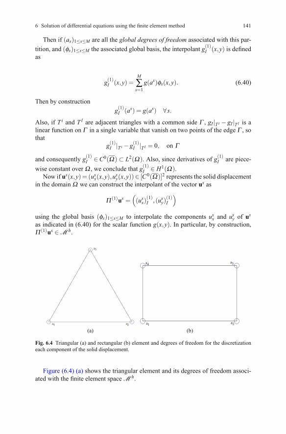
141
Then if (as)1≤s≤M are all the global degrees of freedom associated with this par-
tition, and (φs)1≤s≤M the associated global basis, the interpolant g(1)I (x,y) is definedas
g(1)I (x,y) =M
∑s=1
g(as)φs(x,y). (6.40)
Then by constructiong(1)I (as) = g(as) ∀s.
Also, if T i and T l are adjacent triangles with a common side Γ , gI |T i − gI |T l is alinear function on Γ in a single variable that vanish on two points of the edge Γ , sothat
g(1)I |T i −g(1)I |T l = 0, on Γ
and consequently g(1)I ∈C0(Ω) ⊂ L2(Ω). Also, since derivatives of g(1)I are piece-
wise constant over Ω , we conclude that g(1)I ∈ H1(Ω).Now if us(x,y)= (usx(x,y),u
sy(x,y))∈ [C0(Ω)]2 represents the solid displacement
in the domain Ω we can construct the interpolant of the vector us as
Π (1)us =((usx)
(1)I ,(usy)
(1)I
)using the global basis (φs)1≤s≤M to interpolate the components usx and usy of us
as indicated in (6.40) for the scalar function g(x,y). In particular, by construction,Π (1)us ∈ M h.
a a
a
1 2
3
a a
aa
1 2
34
(a) (b)
Fig. 6.4 Triangular (a) and rectangular (b) element and degrees of freedom for the discretizationeach component of the solid displacement.
Figure (6.4) (a) shows the triangular element and its degrees of freedom associ-ated with the finite element space M h.
6 Solution of differential equations using the finite element method

142
6.13.2 Conforming finite element space over partitions of Ω intorectangular elements to represent solid displacements
Next we define a second finite element space over Ω using bilinear polynomialsover a partition of Ω into rectangles Ri of diameter bounded by h as follows:
LetP1,1 = Span 1,x,y,xy
and set
Note that as in the triangular case, N h ⊂ [H1(Ω)]2, so that N h is a conformingfinite element space of [H1(Ω)]2.
Let us proceed to define the interpolant of a function g(x,y) using the space N h,the argument being similar to that of the triangular case.
For any rectangle R of the partition, if a j, j = 1,2,3,4 are the four vertices ornodes of R, the functions ψ j have the form
ψ j(x,y) = p j+q j x+ r j y+ s j x y, j = 1,2,3,4.
It is immediate to see that the equations
ψk(a j) = δk j, j,k = 1,2,3,4
(6.41)Nh = v= (vx,vy) such that v|Ri ∈ [P1,1(R
j)]2∩
define uniquely four bilinear functions over the rectangle R.Then for any given function g(x,y)∈C0(Ω) we can construct the Lagrange inter-
polant g(1,1)I (x,y) generating a global basis (φs)1≤s≤M as indicated for the triangularcase, by patching together the local basesand Rl with a common node ail being a global degree of freedom.
Then, if (as)1≤s≤M are global degrees of freedom associated with the partition,
g(1,1)I (x,y) =M
∑s=1
g(as)φs(x,y). (6.42)
As in the triangular case, the global basis constructed in this fashion has small sup-port. For boundary nodes, we use as global basis the local basis associated with suchnode.
Also, by construction,
g(1,1)I (as) = g(as) ∀ as.
Thus, if Ri and Rl are adjacent rectangles with a common side Γ , g(1,1)I |Ri −g(1,1)I |Rlis a linear function of a single variable on Γ vanishing on two points of Γ . Thus
ψ ik and ψ l
s of two adjacent rectangles Ri
C0(Ω) .]2[
6.13 2-D finite element spaces

143
g(1,1)I |Ri −g(1,1)I |Rl = 0, on Γ
and consequently g(1,1)I ∈C0(Ω).
Also, since derivatives of g(1,1)I are piecewise constant over Ω , we conclude that
g(1,1)I ∈ H1(Ω).Now for a solid displacement vector us(x,y) = (usx(x,y),u
sy(x,y)) ∈ [C0(Ω)]2
proceeding as before we can construct another interpolant of us as
Π (1,1)us =((usx)
(1,1)I ,(usy)
(1,1)I
),
i.e., we interpolate the components usx and usy of us as indicated in (6.42) for thescalar function g(x,y).
Figure (6.4) (b) shows the rectangular element and its degrees of freedom asso-ciated with the finite element space N h.
To state the interpolation error associated with the above definitions of Π (1)us
and Π (1,1)us we introduce the spaces [H1(Ω)]2 and [H2(Ω)]2 in two dimensions asfollows.
First, for any scalar function v(x,y) defined over Ω we define the norms
‖v‖1 =
(∫Ω
(|v|2 +
∣∣∣∣∂v∂x
∣∣∣∣2 + ∣∣∣∣∂v∂y
∣∣∣∣2)dx
)1/2
, (6.43)
‖v‖2 =
(∫Ω
(|v|2 +
∣∣∣∣∂v∂x
∣∣∣∣2 + ∣∣∣∣∂v∂y
∣∣∣∣2 + ∣∣∣∣∂ 2v∂x2
∣∣∣∣2 + ∣∣∣∣∂ 2v∂y2
∣∣∣∣2 + ∣∣∣∣ ∂ 2v∂x∂y
∣∣∣∣2)dx
)1/2
.
Then we define the spaces [H1(Ω)]2 =H1(Ω)×H1(Ω) and [H2(Ω)]2 =H2(Ω)×H2(Ω) as follows.
[H1(Ω)]2 = v= (vx,vy) :(‖vx‖2
1 +‖vy‖21
)1/2< ∞, (6.44)
[H2(Ω)]2 = v= (vx,vy) :(‖vx‖2
2 +‖vy‖22
)1/2< ∞. (6.45)
Note that the function u(x,y) is interpolated using linear function on each elementof the partition, and derivatives of u(x,y) are interpolated by derivatives of the inter-polants Π (1) or Π (1,1), which are piecewise constants. Then if u(x,y) is sufficientlysmooth (us ∈ [H2(Ω)]2) and the partition of Ω is sufficiently regular, the followingestimates hold [Ciarlet, 1976, Becker et al., 1981]
‖us−Π (1)us‖0 ≤C h2‖u‖2, (6.46)
‖us−Π (1)us‖1 ≤C h‖u‖2, (6.47)
‖us−Π (1,1)us‖0 ≤C h2‖u‖2, (6.48)
‖us−Π (1,1)us‖1 ≤C h‖u‖2, (6.49)
6 Solution of differential equations using the finite element method
144
where C is a positive constant independent of h and h is sufficiently small.
6.13.3 Finite element spaces over rectangular an triangularmeshes to represent fluid displacements
The finite element spaces M h and N h defined above are useful to approximate thesolid displacements of a viscoelastic or poroelastic medium Ω , because displace-ments are continuous across any interior interface Γ of the domain Ω , unless Γ is afracture, where displacements are discontinuous across Γ .
But for computing approximate solutions of Biot’s equations in 2-D or 3-D me-dia, where we must approximate both the solid and fluid vectors, it must be done takinginto account that only the normal component of the fluid displacement is continuousacross any interior interface Γ .
Consequently the spaces M h and N h are not adequate to represent the fluiddisplacement vector and other finite element spaces need to be introduced.
For this purpose, we define first a new space of vector functions H(div,Ω) asfollows
H(div,Ω) = v ∈ [L2(Ω)]2 such that ∇ ·v ∈ L2(Ω). (6.50)
The space H(div,Ω) can be provided with the natural norm
‖v‖H(div,Ω) =(‖v‖2
0 +‖∇ ·v‖20
)1/2. (6.51)
6.13.4 The case of a partition of Ω into rectangular elements
Let us denote by Pk,l to the polynomials of degree not greater than k in x and notgreater than l in y.
Consider a partition T h of Ω into rectangles Ri of diameter bounded by h.Then our first finite element space to approximate the fluid displacement u f in
Biot’s equations is defined as follows:
Vh = v= (vx,vy) ∈ H(div,Ω) such that v|Rj ∈ V
hj , (6.52)
where
Vhj =
[P1,0(R
j)×P0,1(Rj)]. (6.53)
In (6.52) v|Rj indicates the function v as seen from Ω j, and similarly for v|Rk .Remark V h is the vector part of the 2-D Raviart-Thomas-Nedelec
space of zero order [Raviart and Thomas, 1977].
6.13 2-D finite element spaces
. The space

145
It is known that for functions v ∈ V h to have divergence in L2(Ω)sufficient that for any adjacent rectangles Rj and Rk with a common side Γ jk thefollowing condition holds [Nedelec, 1980]
v|Rj ·ν jk+v|Rk ·νk j = 0, on Γjk ∀( j,k). (6.54)
In (6.54) ν jk denote the unit outer normal on Γjk from Rj into Rk, with similarnotation for νk j.
Thus to construct a basis for V h we will patch the local polynomials in adjacentrectangles using (6.54).
First, let R is a rectangle of the partition and Γ any side of R with outer unitnormal νΓ . Note that any v ∈ V h is of the form
v= (vx,vy) = (a+bx,c+dy)
and consequently v ·νΓ is constant on Γ .Let us consider two adjacent rectangles Rj and Rk in T h with a common side
Γ jk = Rj ∩R
k.Assume that by translation and scaling Rj
v|Rj ·ν jk = vx, v|Rk ·νk j =−vx on Γ jk1
and (6.54) implies that vx is continuous on Γ jk1 .
Because the normal component is a constant, we choose the mid point of Γ 1jk =
(0,12) as the common global degree of freedom for the adjacent rectangles Rj and
Rk.Let p j(x,y) = (a+bx,0), pk(x,y) = (c+dx,0); let Γ be any edge of the rectan-
gles Rj,Rk with a common side Γ jk of mid point ξ jk and let νΓ be the unit outernormal to Γ . Then the equations
p j ·ν jk = 1, on Γ jk, p j ·νΓ = 0,Γ = Γ jk,
pk ·νk j = 1, on Γ jk, pk ·νΓ = 0,Γ = Γ jk,
completely determine p j and pk.Let φ x
jk(x,y) the basis function constructed patching p j and pk, with associated
global degree of freedom ξ jk. By construction φ xjk satisfy (6.54), so that φ x ∈ V h.
Let (as)1≤s≤M be the set of global degrees of freedom chosen in this fashion, and(φ x
s )1≤s≤M the associated basis functions in V h.Next we proceed similarly for the y-component vy of v. Assume that by transla-
tion and scaling Rj = [0,1]× [0,−1] and Rk = [0,1]× [0,1], so that Γ jk2 = [0,1]. In
this case ν jk = (0,1) and νk j = (0,−1). Then
v|Rj ·ν jk = vy, v|Rk ·νk j =−vy, on Γ jk2
is necessaryand
so that Γ jk1 = [0,1]. In this case ν jk = (1,0) and νk j = (−1,0). Then
= [−1,0]× [0,1] and Rk= [0,1]× [0,1],
6 Solution of differential equations using the finite element method

146
and (6.54) implies that vy is continuous on Γ jk2 .
Because the normal component is a constant, we choose the mid point of Γ 2jk =
(12,0) as the common global degree of freedom for Rj and Rk.
Let p j = (0,a+ by), pk = (0,c+ dy); let Γ be any side of the rectangles Rj,Rk
with a common side Γ jk of mid point ξ jk and νΓ the unit outer normal to Γ . Theequations
p j ·ν jk = 1, on Γ jk p j ·νΓ = 0,Γ = Γ jk,
pk ·νk j = 1, on Γ jk pk ·νΓ = 0,Γ = Γ jk,
completely determine p j and pk.Let φ y
jk the basis function element constructed patching p j and pk, with associ-ated global degree of freedom ξ jk.
By construction φ yjk satisfy (6.54), so that φ y
jk ∈ V h.Let (bs)1≤s≤N be the set of all global degrees of freedom selected in this way and
(φ ys )1≤s≤N the associated basis functions in V h.Then we define the interpolant Q(1,1)u f ∈ V h of the fluid displacement vector as
Q ,1)u f =
(M
∑s=1
u fx (as)φ x
s (x,y),N
∑t=1
u fy (bs)φ y
s (x,y)
).
The following interpolation error estimates hold [Raviart and Thomas, 1977,Nedelec, 1980]
(6.55)
6.13.5 The case of a partition of Ω into triangular elements
Next we construct a finite element space to approximate the fluid displacement overa partition of T h of Ω into triangles T i of diameter bounded by h. We first definethe set
S2 = (P0,P0)+(xP0,yP0), (6.56)
to be used on each triangle T i. Here P0 denotes the constants.Note that any element w ∈ S2 is of the form
w= (a+ cx,b+ cy), a,b,c constants. (6.57)
If follows immediately from (6.57) that for any side Γ of a triangle T ∈ T h withunit outer normal νΓ and w ∈ S2
(1
‖u f −Q ,1)u f ‖0 ≤Ch ‖u f ‖0
‖u f −Q ,1)u f ‖H(div,Ω) ≤Ch ‖u f ‖H(div,Ω).
(1
(1
6.13 2-D finite element spaces

147
w ·νΓ (6.58)
is constant.The finite element space over the partition T h of Ω into triangles is defined as
Wh = w= (wx,wy) ∈ H(div,Ω) such that w|T j ∈ S2.
ϕ j ·νΓ k = δ jk, j,k = 1,2,3.
Also, we choose as global degrees of freedom the common mid point of two adjacenttriangles.
As in the rectangular case, we construct a global basis for the space W h by patch-ing two adjacent triangles. The argument is identical to the rectangular case and isomitted.
a1 a
a
3
2
a1
a2
a3
a4
(a) (b)
Fig. 6.5 Triangular (a) and rectangular (b) elements and degrees of freedom for the discretizationof the fluid displacement.
Figure (6.5) shows the triangular (a) and rectangular (b) elements and its degrees
6.14 3-D Finite element spaces
Here we briefly describe the finite element spaces used later to represent solid andfluid vectors in three dimensions.
Next, thanks to (6.58), on each triangle T with sides Γ i and unit outer normalsνΓ i , i=1,2,3 the following three equations define uniquely three local bases1,2,3 in the space S2:
ϕ j, j =
of freedom associated with the finite element spaces andW h , respectively.V h
6 Solution of differential equations using the finite element method

148
6.14.1 Conforming finite element spaces to represent the soliddisplacement using tetrahedral and 3-rectangular elements
First let us consider a bounded domain Ω ⊂ R3 and a partition T h of Ω into tetra-hedra T i.
Let us define the finite element space as follows:
ϕ j(x,y,z) = a j+b j x+ c j y+d j z, j = 1,2,3,4.
The values of the polynomial ϕ j(x,y) at the four nodes of the tetrahedron T are thelocal degrees of freedom and they uniquely define the polynomial ϕ j(x,y,z).
Thus, the equations
ϕk(a j) = δk j, j,k = 1,2,3,4 (6.59)
uniquely define four linear functions ϕk(x,y,z),k= 1,2,3,4 over the tetrahedron T ;they are a local basis over T .
Now for an element v= (vx,vy,vz) ∈ M h a global basis
(φ xj )1≤ j≤J, (φ y
k )1≤k≤K , (φ zl )1≤l≤L
to represent vx,vy and vz, respectively, is constructed by patching together the localbasis of the form in (6.59) of adjacent tetrahedra.
Then the functions
Φ j k l =(φ xj ,φ
yk ,φ
zl
), j = 1, · · · ,J, k = 1, · · · ,K, l = 1, · · ·L
are a global basis for M h.Let us consider now the case in which the domain Ω is partitioned into 3-
rectangles Ri. First, we define the local polynomials on any 3-rectangle R as
Q1 = Span(1,x,y,z,xy,xz,yz,xyz) .
SincedimQ1 = 8,
for any 3-rectangle R in the partition we choose as local degrees of freedom the eightvertices a j of R.
Next, for any polynomial ψk ∈ Q1, the equations
6.14 3-D Finite element spaces
Mh = v= (vx,vy,vz) : v|T i ∈ [P1(T
i)]3∩
where P1(T i) denotes the polynomials of degree less or equal to 1 in the variables(x,y,z). Note that M h is a conforming finite element space of [H1(Ω)]3.
For any tetrahedron T of the partition, if a j = (x j,y j,z j), j= 1,2,3,4 are the fourvertices, to be referred also as nodes of T , the functions ϕ j ∈ P1(T ) have the form
C0(Ω) ,]3[

149
ψk(a j) = δk j, j,k = 1, · · · ,8 (6.60)
uniquely define eight functions ψk(x,y,z),k = 1, . . . ,8, over the 3-rectangle R; theyare a local basis for R.
Now we define the finite element space over the 3-rectangular finite elementpartition as
Nh = v= (vx,vy,vz) such that v|Ri ∈ [Q1]
3∩C0(Ω). (6.61)
As in the case of tetrahedral elements, a global basis for the space N h in (6.61)is constructed by patching together the local basis of the form in (6.60) of adjacenttetrahedra for each component of an element v= (vx,vy,vz) ∈ N h in (6.61).
Figure (6.6) shows the 3-rectangular elements (a) and tetrahedral (b) to discretize
a a
a a
a a
a a
1 2
5 6
78
34
a
a
a
a
1
2
3
4
(a) (b)
Fig. 6.6 3-rectangular (a) and tetrahedral (b) elements and degrees of freedom for the 3-D solid
6.14.2 Finite element spaces to represent the fluid displacementusing 3-rectangular and tetrahedral elements
Next we define the finite element space to approximate fluid displacement vectorsin R3, as a natural extension to those in the 2-D case.
Let
H(div,Ω) = v ∈ [L2(Ω)]3 such that ∇ ·v ∈ L2(Ω). (6.62)
The space H(div,Ω) is provided with the norm defined in (6.51).
the solid displacement vector associated with the spaces andN h , respectively.M h
displacement discretization associated with the spaces andN h , respectively.M h
6 Solution of differential equations using the finite element method
Remark M h and N h are conforming finite element spaces of [H1(Ω)]3.. Both

150
Consider a partition T h of Ω into 3-rectangles Ri of diameter bounded by h andlet Pj,k,l denote the polynomials of degree not greater than j in x, not greater than kin y and not greater than l in z.
The finite element space defined over the partition T h to approximate the fluiddisplacement u f in Biot’s equations is defined as
Yh = v= (vx,vy,vz) ∈ H(div,Ω) such that v|Rj ∈ [P1,0,0 ×P0,1,0 ×P0,0,1].
Note if v ∈ Y h, for any face Γ with unit outer normal νΓ of a 3-rectangle R of the
Hence as in the 2-D case, we use (6.54) to construct a global basis function forY h by patching the local basis of adjacent 3-rectangles, choosing the mid points ofthe faces of such 3-rectangles as global degrees of freedom.
to construct Q(1,1) in the 2-D case and is omitted.Next we construct a finite element space to approximate the fluid displacement
over a partition T h of Ω into tetrahedra T i of diameter bounded by h. Let
S3 = (α1,α2,α3)+β (x,y,z), α1,α2,α3,β ∈ P0.
Then we define
Zh = v= (vx,vy,vz) ∈ H(div,Ω) such that v|T j ∈ S3.
Note that for any tetrahedron T in the partition T h, an element v∈ S3 is uniquelydetermined by the (constant) values of its normal components on the four faces ofT [Nedelec, 1980]. Thus the nodes are chosen to be the four mid points of the facesof T .
A global basis for Z h can be constructed as indicated above for the 3-rectangularcase.
Figure (6.7) shows the 3-rectangular (a) and tetrahedral (b) elements associatedwith the spaces Y h and Z h.
6.15 Non-conforming finite element spaces to represent soliddisplacements in 2-D and 3-D
Non-conforming finite element spaces will be used to represent the solid displace-ment vector when solving wave propagation problems in two and three dimen-sions. This choice is explained by the fact that they induce less numerical dis-persion as compared with the conforming spaces described in the previous section[Zyserman et al., 2003, Zyserman and Gauzellino, 2005].
An additional advantage is that non-conforming spaces require less amount ofinformation to be passed among processors in any parallel implementation of thealgorithms to be described in the next sections.
partition, v ·νΓ is constant on Γ.
The construction of the interpolation operator Q(1,1,1)u ∈ follows the ideasY h
6.15 Non-conforming finite element spaces to represent solid displacements in 2-D and 3-D

151
a1
a 2
a3
a4
a 5
a6a1
a 2
a 3
a4
(a) (b)
Fig. 6.7 3-rectangular (a) and tetrahedral (b) elements and degrees of freedom for the 3-D fluiddisplacement discretization associated with the spaces Y h and Z h, respectively.
Thus we include here the description of the non-conforming spaces in 2-D and 3-D to be used. These spaces have been defined and analyzed in [Douglas Jr. et al., 1999,Douglas Jr. et al., 2001].
6.15.1 The case of a partition of Ω into n-simplices
First consider the case that the domain Ω ⊂ Rn, n=2,3, is partitioned into trianglesor tetrahedra T i, referred to a n-simplices, of diameter bounded by h. Let
Γ j = ∂Ω ∩∂T j, Γ jk = ∂T j ∩∂Tk.
Let ξ j and ξ jk denote the mid points of the faces of Γ j and Γ jk, respectively.Then we define the local finite element polynomials as
N Chi = [P1(T
i)]n, n= 2,3.
The local degrees of freedom are chosen to be the three centers of the sides of thetriangle T i for n=2, and the four centers of the faces of the tetrahedron T i for n= 3.
Then the finite element space defined over the partition of Ω in n-simplices isdefined as
N Ch = v such that v j = v|T j ∈ N C
hj , v j(ξ jk) = vk(ξ jk), ∀ j,k. (6.63)
A local basis can be constructed by requiring at each local basis function to take thevalue one at one nodal point ξ j or ξ jk and and zero at all other nodal points.
Then a global basis for N Ch is obtained patching together the local basis of sim-
plices having a common side (triangles) or a common face (tetrahedron). Boundarynodes are treated as in the 2-D case.
6 Solution of differential equations using the finite element method

152
Note that the elements in N Ch are functions in [L2(Ω)]n, but since continuity
across the interfaces Γ jk is required only at the mid points ξ jk of inter-element facesΓ jk, functions in N C
h do not have first derivatives in [L2(Ω)]n, so that N Ch is
NOT a subset of [H1(Ω)]n.In this case it is said that N C
h is a non-conforming finite element space of[H1(Ω)]n.
Next, for any vector function u sufficiently smooth defined over Ω , we may con-struct the interpolation operator Πu∈N C
h using the values of u at the nodal pointsand the global basis in N C
h.Since Π reproduces constants and linears on each element T i of the finite element
partition, the interpolation error in the L2-norm can be estimated as [Douglas Jr. et al.,
‖u−Πu‖0 ≤Ch2‖u‖2. (6.64)
In (6.64) the [H2(Ω)]3-space is defined for vector functions defined over Ω ⊂ R3
asking that all first and second derivatives on the three space variables of all com-ponents of the vector be square integrable. Then the norm in [H2(Ω)]3 is definedsimilarly to that defined in (6.43) for 2-D vector functions.
6.15.2 The case of a partition of Ω into n-rectangles
Next consider the case in which the domain Ω ⊂ Rn, n=2,3, is partitioned into n-rectangles Ri.
Consider first the case n = 2 and the reference rectangle R = [−1,1]2 and thereference basis
P(R) = Span1,x,y,θ(x)−θ(y), θ(ζ ) = ζ 2 − 53
ζ 4. (6.65)
The four local degrees of freedom associated with (6.65) are the values at the centersof the sides of R.
In the case n= 3, we take a reference element R= [−1,1]3 and a reference basis
P(R) = Span1,x,y,z,θ(x)−θ(y),θ(x)−θ(z), θ(ζ ) = ζ 2 − 53
ζ 4. (6.66)
The six local degrees of freedom associated with (6.66) are the values at the centersof the faces of R.
Consider now a partition T h of the domain Ω into n-rectangular elements Rj
and setMC
hj = [P(Rj)]n, n= 2,3. (6.67)
Then the finite element space defined over a partition of Ω into n-rectangles isdefined as
MCh = v such that v j = v|Rj ∈ MC
hj , v j(ξ jk) = vk(ξ jk), ∀ j,k. (6.68)
1999]
6.15 Non-conforming finite element spaces to represent solid displacements in 2-D and 3-D

153
Note that the space MCh defined in (6.68) is also a non-conforming finite space of
[H1(Ω)]n for the same reason that the space over n-simplices defined in (6.63).A global basis for MC
h and an interpolation operator can be constructed asindicated for the case of n-simplices. Also, the interpolation error stated in (6.64)for the n-simplices case is still valid for the n-rectangular case.
6 Solution of differential equations using the finite element method

Chapter 7
Modeling Biot media at the meso-scale using afinite element approach
Abstract Fast compressional or shear waves travelling through a fluid-saturatedporous material (a Biot medium) containing heterogeneities on the order of cen-timeters (mesoscopic scale) suffer attenuation and dispersion observed in seismicdata. The mesoscopic loss effect occurs because different regions of the mediummay undergo different strains and fluid pressures. This in turn induces fluid flow andBiot slow waves causing energy losses and velocity dispersion. Numerical model-ing of wave propagation using Biot’s equations of motion takes into account thisphenomenon but is computationally very expensive. In the context of NumericalRock Physics, this chapter presents compressibility and shear time-harmonic ex-periments to determine an equivalent viscoelastic medium having in the averagethe same attenuation and velocity dispersion than the original highly heterogeneousBiot medium. Each experiment is associated with a boundary-value problem that issolved using the finite element method.
7.1 Introduction
A major cause of attenuation and velocity dispersion in Biot media is wave-inducedfluid flow, which occurs at the mesoscopic scale, on the order of centimeters, but itseffect can be observed at the macro-scale.
The loss mechanism predicted by Biot’s theory [Biot, 1956a, Biot,1956b, Biot,1962],the classical Biot’s global fluid flow in homogeneous media, has a macroscopic na-ture and is due to wavelength-scale fluid pressure equilibration between the peaksand troughs of the fast propagating waves. This induces a relative displacementbetween the solid frame and the fluid, causing energy dissipation due to viscousfriction. Although the attenuation due to global flow is generally important in therange of ultrasonic frequencies, it is not significant in the seismic frequency band.
In Biot’s theory the attenuation peak moves to high frequencies with increas-ing viscosity and decreasing permeability. Thus at low frequencies, attenuation de-
© Springer International Publishing AG 2016
in Geosystems Mathematics and Computing, DOI 10.1007/978-3-319-48457-0_7
155J.E. Santos, P.M. Gauzellino, Numerical Simulation in Applied Geophysics, Lecture Notes

156
creases with increasing viscosity or decreasing permeability, contradicting experi-mental data [Jones, 1986].
To explain low-frequency seismic or sonic attenuation in rocks, a non-Biot atten-uation mechanisms called squirt flow has been suggested and analyzed by severalauthors [O’Connell and Budiansky, 1974, Dvorkin et al., 1995, Mavko et al., 1998].However, [Pride et al., 2004] has shown that squirt flow can not describe the ob-served levels of dissipation at seismic frequencies.
Pride and coauthors [Pride et al., 2004] have shown that attenuation and velocitydispersion measurements at seismic frequencies can be explained by wave-inducedfluid flow at mesoscopic scales and energy transfer between wave modes. They referto this mechanism as mesoscopic loss.
The mesoscopic scale refers to heterogeneities in the rock and fluid propertiesgreater than the pore size but much smaller than the wavelengths of the fast com-pressional and shear waves.
Basically, when a compressional wave travels through an heterogeneous fluid-saturated porous material, the different regions may undergo different strains andfluid pressures. This in turn generates fluid flow and diffusive Biot slow waves in-ducing energy losses and velocity dispersion.
White and coauthors [White et al., 1975] were the first to model the wave-induced fluid flow caused by mesoscopic-scale heterogeneities, showing that thismechanism causes important attenuation and velocity dispersion effects at seis-mic frequencies in partially saturated rocks. They obtained approximated solutionsof the response of plane porous layers alternately saturated with gas and water[White et al., 1975] and of spherical gas pockets in a water-saturated porous rock[White, 1975].
Later, several authors proposed other analytical models to explain the response offluid-filled porous materials containing specific mesoscopic-scale heterogeneities.We mention [Dutta and Ode, 1979], that analyzed attenuation and dispersion effectsin a Biot medium with partial gas saturation. Also, [Pride and Berryman, 2003] whoobtained an analytical model for the seismic response of a mixture of two dif-ferent porous phases having a single dominant length scale, while [Norris, 1993]and [Gurevich and Lopatnikov, 1995] focused on the case of layered porous me-dia. A generalization of White model for patches of arbitrary shape appeared in[Johnson, 2001]. This model has two geometrical parameters, the specific surfacearea and the size of the patches.
The mesoscopic phenomenon was analyzed in the laboratory in the paper by[Cadoret et al., 1995] at the frequency range 1–500 kHz, observing different veloc-ities for either drainage or imbibition saturation procedures. Using computerizedtomography (CT) scans, it was possible to visualize the fluid distribution and spatialheterogeneities in real rocks.
Mesoscopic effects have also been studied using numerical simulations of wavepropagation. The work by [Carcione et al., 2003] presents numerical simulationsbased on Biot’s equations of poroelasticity and White model of regularly distributedspherical gas inclusions. The experiments show that the mesoscopic loss effect can
7.1 Introduction

157
be explained by the combined effect of mesoscopic-scale inhomogeneities and en-ergy transfer between wave modes.
Also, fractals models calibrated by computed tomography (CT) scans to modelheterogeneities in Biot media and perform numerical simulations can be found in[Helle et al., 2003]. Later, the work by [Muller and Gurevich, 2005] analyzed theasymptotic behaviour of attenuation and dispersion versus frequency in differentrandom porous media. Besides, [Toms et al., 2007] studied the mesoscopic effectsin the case of continuous random fluid distributions and [Muller and Toms, 2007]focused on fractal fluid distributions.
The wave propagation experiments using a finite element method presented in[Rubino et al., 2007] show the numerical evidence of the mesoscopic loss mecha-nism in the seismic range of frequencies for the White model of alternating layersof poroelastic rocks saturated with either gas or water.
Using a numerical approach to model wave propagation using Biot’s equationsof motion allows to model heterogeneities of any kind and shape. However, thismethodology is computationally expensive or even not feasible due to different rea-sons. First, even in the hypothetical case in which the exact spatial distribution of thedifferent constituents would be known, very fine meshes would be needed to repre-sent the heterogeneities. In addition, in the low frequency range the resolution of thediffusion process associated with the fluid pressure equilibration is a critical issue,since the diffusion length is very small as compared with the seismic wavelengths.
To overcome these limitations, a different approach was presented by [Masson andwhere a time-varying stress is applied to the boundaries of an hetero-
and determined its effective complex moduli by numerically com-stress and strain fields.
This chapter describes a finite element procedure combined with a Montecarloapproach to obtain the effective complex P-wave and shear moduli in Biot mediawith heterogeneities in the fluid and petrophysical properties described by stochas-tic fractals. This approach allows us to determine an effective isotropic viscoelasticmedium behaving in the average like the original medium. Since a viscoelastic solidis neither able to represent the propagation of both fast and slow waves nor sup-port fluid flow through it, this equivalence must be understood in the previouslymentioned sense.
The procedure consists in applying time-harmonic compressibility and shearstresses to numerical rock samples associated with a given realization of the stochas-tic parameters at a finite number of harmonic frequencies. The complex moduli arecalculated by defining locally an equivalent viscoelastic solid having the same atten-uation and velocity dispersion than the original fluid-saturated porous rock. Biot’stheory [Biot, 1962] is used to model the response of the heterogeneous material tothe applied stresses.
The procedure is a generalization of the ideas presented in [White et al., 1975]and [White, 1975] to explain the attenuation effects suffered by compressionalwaves travelling in partially saturated rocks for the idealized cases of alternatinglayers saturated either with gas or water or for a water saturated rock containingspherical gas pockets.
Pride, 2007],geneous sampleputing the average
7 Modeling Biot media at the meso-scale using a finite element approach

158
For each realization of the stochastic parameters, the complex moduli are ob-tained by solving Biot’s equations in the space-frequency domain in the diffusiverange of frequencies using a finite element procedure.
Appropriate boundary conditions are used to represent compressibility and shearlaboratory experiments.
These complex moduli in turn allow us to obtain the corresponding equivalentcompressional and shear phase velocities and quality factors for each frequency andrealization.
The statistical properties of the computed equivalent phase velocities and inversequality factors are obtained by averaging over the realizations of the stochastic pa-rameters. The Montecarlo realizations are stopped when the variance of the com-puted quantities stabilizes at an almost constant value.
In this fashion we determine the complex and frequency dependent moduli in theconstitutive relations of an isotropic effective viscoelastic medium behaving in theaverage as our original highly-heterogeneous Biot medium.
The numerical procedure presented can be regarded as an up-scaling method toobtain the effect of the mesoscopic scale heterogeneities at the macro-scale.
For the compressional case the algorithm was validated comparing the resultswith those obtained using a White’s model which is valid for alternating layers oftwo fluid-saturated porous sandstones ([White, 1975]). For the shear case, the algo-rithm was checked to yield the real shear modulus for the case of uniform either gasor water saturation at the zero frequency limit.
7.2 Determination of the complex P-wave and shear moduli ofthe equivalent viscoelastic medium
Here we describe the experiments to determine the equivalent complex plane-waveand shear moduli of a highly heterogeneous Biot medium.
These experiments consist of applying time-harmonic compressional and shearstresses to a representative sample of a fluid-saturated porous rock. As mentioned
This procedure is implemented computationally in the 2-D case, with the obviousextension to the 3-D case.
Recall the frequency-domain stress-strain relations in a Biot medium:
τkl(u) = 2μ εkl(us)+δkl(λu ∇ ·us+B∇ ·u f ) , (7.1)
p f (u) =−B∇ ·us−M∇ ·u f , (7.2)
where u= (us,u f ), us = (us1,us3),u
f = (u f1 ,u
f3).
In (7.1)-(7.2), to simplify notation we omit the symbol Δ in front of the stress τand the fluid pressure p f appearing in the derivation of these constitutive relationsin Chapter 1 equations (1.16)-(1.17).
7.2 Determination of the complex P-wave and shear moduli of the equivalent viscoelastic medium
before, the theoretical framework for this procedure was given in the works of [WhiteWhite, 1975, Dutta and Od´ e, 1979] and [Johnson, 2001].1975,et al.,

159
Biot’s equations in the diffusive range (ignoring acceleration terms) are (seeChapter 1, equations (1.79)-(1.80)
∇ · τ(u) = 0, (7.3)
iωηκ−1u f +∇p f (u) = 0, (7.4)
where η is the fluid viscosity and κ is the frame permeability.Equations (7.3)-(7.4) will be solved in the 2-D case on square sample Ω = (0,L)2
with boundary Γ = ∂Ω in the (x1,x3)-plane. The domain Ω is a representativesample of our fluid saturated poroelastic material.
Set Γ = Γ L∪Γ B∪Γ R∪Γ T , where
Γ L = (x1,x3) ∈ Γ : x1 = 0, Γ R = (x1,x3) ∈ Γ : x1 = L,Γ B = (x1,x3) ∈ Γ : x3 = 0, Γ T = (x1,x3) ∈ Γ : x3 = L.
Denote by ν the unit outer normal on Γ and let χ be a unit tangent on Γ orientedcounterclockwise so that ν ,χ is an orthonormal system on Γ .
For obtaining the complex plane wave modulus of our fluid-saturated porousmedium, let us consider the solution of (7.3)-(7.4) with the following boundaryconditions
τ(u)ν ·ν =−ΔP, (x1,x3) ∈ Γ T , (7.5)
τ(u)ν · χ = 0, (x1,x3) ∈ Γ , (7.6)
us ·ν = 0, (x1,x3) ∈ Γ L∪Γ R∪Γ B, (7.7)
u f ·ν = 0, (x1,x3) ∈ Γ . (7.8)
For this set of boundary conditions the solid is not allowed to move normally to thelateral and bottom boundaries, the fluid is not allowed to flow out of the sample,a uniform compression is applied on the boundary Γ T and no tangential externalforces are applied on the boundary Γ .
These boundary conditions can be associated with a laboratory experiment fora periodic sample obtained by a mirror reflection with respect to the x1-axis of thedomain Ω , enclosing the periodic sample in a thin impermeable jacket and applyinga uniform compression on the boundary Γ T and its corresponding image boundaryafter the indicated reflection. In the case of periodic layered media, this experimentmimics exactly the one described in [White et al., 1975].
Denoting by V the original volume of the sample, its (complex) oscillatory vol-ume change ΔV (ω) allows us to define the equivalent undrained complex plane-wave modulus Eu(ω), by using the relation
ΔV (ω)
V=− ΔP
Eu(ω), (7.9)
valid for a viscoelastic homogeneous medium in the quasi-static case.
)
7 Modeling Biot media at the meso-scale using a finite element approach

160
After solving (7.3)-(7.4) with the boundary conditions (7.5)-(7.8), the averagevertical displacement us,T3 (ω) of the vertical solid displacements us3(x1,L,ω) on Γ T
is computed.Then, for each frequency ω , the complex volume change produced by the com-
pressibility test can be approximated by
ΔV (ω)≈ Lus,T3 (ω),
which enables us to compute the equivalent complex plane-wave modulus Eu(ω)from (7.9).
The corresponding complex compressional velocity is
vpc(ω) =
√Eu(ω)
ρ,
where ρ is the average bulk density of the sample.The following relations allow us to estimate the equivalent compressional phase
velocity vp(ω) and quality factor Qp(ω) in the form
vp(ω) =
[Re
(1
vpc(ω)
)]−1
,1
Qp(ω)=
Im(vpc(ω)2)
Re(vpc(ω)2). (7.10)
Figure 7.1 shows a schematic representation of the undrained oscillatory com-pressibility test.
Fig. 7.1 The harmonic com-pressibility test applied toa representative sample ofsaturated poroelastic mate-rial. The boundary conditionsrepresent a normal stressapplied on the top bound-ary, no tangential stresses onall boundaries and no fluidis permitted to flow into orout of the sample. Also, thesolid is not allowed to movenormally to the lateral andbottom boundaries.
Pe )iwtσν = (0,−Δ
7.2 Determination of the complex P-wave and shear moduli of the equivalent viscoelastic medium

161
For obtaining the equivalent complex shear modulus of our fluid-saturated porousmedium, let us consider the solution of (7.3)-(7.4) with the following boundaryconditions
−τ(u)ν = g, (x1,x3) ∈ Γ T ∪Γ L∪Γ R,
us = 0, (x,y) ∈ Γ B,
u f ·ν = 0, (x,y) ∈ Γ ,
where
g=
⎧⎪⎪⎪⎪⎨⎪⎪⎪⎪⎩(0,ΔG), (x1,x3) ∈ Γ L,
(0,−ΔG), (x1,x3) ∈ Γ R,
(−ΔG,0), (x1,x3) ∈ Γ T .
The change in shape of the rock sample allows to recover its equivalent complexshear modulus μc(ω) by using the relation
tg(θ(ω)) =ΔT
μc(ω), (7.11)
where θ(ω) is the departure angle between the original positions of the lateralboundaries and those after applying the shear stresses (see, for example, [Kolsky, 1963]).Equation (7.11) holds for this experiment in a viscoelastic homogeneous media inthe quasi-static approximation.
Computing the average horizontal displacement us,T1 (ω) of the horizontal dis-placements us1(x1,L,ω) at the top boundary Γ T yields an approximation to thechange in shape suffered by the sample, given by
tg(θ(ω))≈ us,T1 (ω)/L.
Then from (7.11) the shear modulus μc(ω) is obtained.The complex shear velocity is given by
vsc(ω) =
√μc(ω)
ρ
and the equivalent shear phase velocity vs(ω) and (inverse) quality factor Qs(ω) areestimated using the relations
vs(ω) =
[Re
(1
vsc(ω)
)]−1
,1
Qs(ω)=
Im(vsc(ω)2)
Re(vsc(ω)2). (7.12)
Figure 7.2 shows and illustration for the undrained shear experiment.
7 Modeling Biot media at the meso-scale using a finite element approach

162
Fig. 7.2 The harmonic sheartest applied to a representativesample of saturated poroe-lastic material. The figureshows the application of shearstresses on the left, right, andtop boundaries. The solid isnot allowed to move on thebottom boundary, and no fluidis permitted to flow into or outof the sample.
σν = (ΔTe ,0)iwt
σν
= (
0,−
Δiw
tT
e )
σν
= (
0,Δ
Te
)iw
t
7.3 A variational formulation
First we introduce the following functional spaces that are closed subspaces of thespaces [H1(Ω)]2 and H(div;Ω) defined in (6.44) and (6.50).
H1,P(Ω) = v ∈ [H1(Ω)]2 : v ·ν = 0 on Γ L∪Γ R∪Γ B,
H1,T0,B (Ω) = v ∈ [H1(Ω)]2 : v= 0 on Γ B,
H0(div,Ω) = v ∈ [L2(Ω)]2 : ∇ ·v ∈ L2(Ω),v ·ν = 0 on Γ .Next, let us define the spaces
V(P) =
[H1,P(Ω)
]2 ×H0(div;Ω), V(T ) =
[H1,T
0,B (Ω)]2
×H0(div;Ω).
Then multiply equation (7.3) by a test function vs ∈ [H1,P(Ω)]2
and equation (7.4)by a test function v f ∈ H0(div;Ω), integrate over Ω , use integration by parts andapply the boundary conditions (7.5)-(7.8). Adding the resulting equations we seethat the solution u(P) = (u(s,P),u( f ,P)) ∈ V (P) of (7.3)-(7.4) and (7.5)-(7.8) satisfiesthe weak form:
Λ(u(P),v) =−〈ΔP,vs ·ν〉Γ T , ∀ v=(vs,v f ) ∈ V
(P), (7.13)
where the bilinear form Λ(u,v) is defined by
7.3 A variational formulation

163
Λ(u,v) = iω(η κ−1u f ,v f )+∑
l,m
(τlm(u),εlm(vs))−(p f (u),∇ ·v f )
= iω(η κ−1u f ,v f )+(D ε(u), ε(v)) . (7.14)
In (7.13) for f ,g either scalar or vector functions and Γ ∗ any subset of Γ we use thenotation
〈 f ,g〉Γ ∗ =∫
Γ ∗f gd(Γ ∗).
Also, the matrix D and the column vector ε((u)) in (7.14) are defined by
D=
⎛⎜⎜⎝λu+2μ λu B 0
λu λu+2μ B 0B B M 00 0 0 4μ
⎞⎟⎟⎠ , ε(u) =
⎛⎜⎜⎝ε11(us)ε33(us)∇ ·u f
ε13(us)
⎞⎟⎟⎠ . (7.15)
The term (D ε(u), ε(v)) in (7.14) is associated with the strain energy of our sys-tem, so that the matrix D must be positive definite. The positive definitess of Dfollows assuming that the entries in the matrix D satisfy the conditions in (1.58)derived in Chapter 1.
Similarly, the solution u(T ) = (u(s,T ),u( f ,T )) ∈ V (T ) of (7.3)-(7.4) and (7.11)-(7.11) satisfies the weak form:
Λ(u(T ),v) =−〈g,vs〉Γ \Γ B , ∀ v=(vs,v f ) ∈ V
(S). (7.16)
Existence of the solution of the boundary value problem (7.3)-(7.4) and either(7.5)-(7.8) or (7.11)-(7.11) and its variational formulations (7.13) or (7.16) will beassumed.
The proof of uniqueness of the solution of the variational problems (7.13) and(7.16) is given in Appendix 7.10.
7.4 The finite element procedures
Let T h(Ω) be a non-overlapping partition of Ω into rectangles Rj of diameterbounded by h such that Ω = ∪J
j=1Rj.
The solid displacement vectors are represented using closed subspaces of thefinite element space N h defined in (6.41).
These finite element spaces, denoted N h,P ⊂ H1,P(Ω) and Nh,T
0,B ⊂ H1,T0,B (Ω)
are used to represent the solid displacement vector for the compressibility and sheartests models, respectively. They are defined as follows
Nh,P = v : v|Rj ∈ [P1,1(R
j)]2, v ·ν = 0 on Γ L∪Γ R∪Γ B∩ [C0(Ω)]2,
Nh,T
0,B = v : v|Rj ∈ [P1,1(Rj)]2, v= 0 on Γ B∩ [C0(Ω)]2.
7 Modeling Biot media at the meso-scale using a finite element approach

164
[H1(Ω)]2. Also note that the boundary conditions (7.7)-(7.8) and (7.11)-(7.11) havebeen imposed strongly on the spaces N
h,P and Nh,T
0,B , respectively.
To approximate the fluid displacement a closed subspace V h0 of the finite element
space V h defined in (6.52) is used. It is defined as
Vh
0 = v : v|Rj ∈ P1,0 ×P0,1, v ·ν = 0 on Γ .
Let us introduce the finite element spaces
V(h,P) = N
h,P×Vh
0 , V(h,T ) = N
h,T0,B ×V
h0 .
Then the finite element procedure to compute the approximate solution of u(P)
(7.13) is defined as follows: find u(h,P) =(u(s,h,P),u( f ,h,P)
)∈ V h,P such that
Λ(u(h,P),v) =−〈ΔP,vs ·ν〉Γ T , ∀ v=(vs,v f ) ∈ V
(h,P). (7.17)
In a similar fashion, the finite element procedure to compute the approximate
solution u(T ) of (7.16) is: find u(h,T ) =(u(s,h,T ),u( f ,h,T )
)∈ V (h,T ) such that
Λ(u(h,T ),v) =−〈g,vs〉Γ \Γ B , ∀ v=(vs,v f ) ∈ V
(h,T ). (7.18)
Since u(h,P) ∈H1,P and u(h,T ) ∈H1,T0,B , uniqueness for the discrete problems (7.17)
and (7.18) follows from the uniqueness for the continuous case demonstrated inTheorem 7.3 in Appendix 7.10. Existence follows from finite dimensionality. Thisresult is stated in the following theorem.
Theorem 7.1. There exists a unique solution of problems (7.17) and (7.18) for anyω > 0 under the assumption that the coefficients in the constitutive relations (7.1)-(7.2) satisfy the conditions in (1.58).
7.4.1 Error estimates for the finite element procedures
The a priori error estimates for the procedures (7.17) and (7.18) can be found in[Santos and Carcione, 2015]. The result is stated in the following theorem.
Theorem 7.2. Assume that the coefficients in the constitutive relations (7.1)-(7.2)satisfy the conditions stated in (1.58). Then for any ω > 0 the solutions u(h,P),u(h,T )
of problems (7.17) and (7.18) satisfy the following a priori error estimates
‖u(s,h, j)−u(s, j)‖1 +‖u( f ,h, j)−u( f , j)‖0 +‖∇ ·(u( f ,h, j)−u( f , j)
)‖0 (7.19)
≤C(ω)[h1/2‖u(s, j)‖3/2 +h
(‖u( f , j)‖1 +‖∇ ·u( f , j)‖1
)], j = P,T.
7.4 The finite element procedures
Remark N h,P and Nh,T
0 B are conforming finite element spaces of. Note that ,

165
Sobolev space [H3/2(Ω)]2 of functions having 3/2 derivatives in Ω . We refer to[Adams, 1975] for a precise definition of the definition of Sobolev spaces of frac-tional order.
Concerning choice of the mesh size h, it has to be small enough so that diffusionprocess associated with the fluid pressure equilibration is accurately resolved.
Recall that the diffusion length is given by the relation length [Mavko et al., 1998]
Ld =
√2πκKf
ηω. (7.20)
For practical purposes, we take h so that the minimum diffusion length is discretizedwith at least 3 mesh points at the highest frequency, which is sufficient to representa (smooth) diffusion-type process.
Besides, the size of the rock sample is not arbitrary: it has to be big enough toconstitute a representative part of the Biot medium but, at the same time, it has tobe much smaller than the wavelengths associated with each frequency.
To find an upper bound for the side length L of the sample, it was checked thatthe compressibility and shear tests applied to homogeneous samples of side lengthL, composed of any of the different materials forming the heterogeneous medium,give negligible attenuation and velocity dispersion at the highest frequency beingconsidered.
7.5 A Montecarlo approach for stochastic fractal parameterdistributions
Field measurements show that permeability values in reservoir rocks have a highdegree of spatial variability and exhibit long range correlations. It is also known thatthese permeability fluctuations are well described by stochastic fractals [Douglas Jr.
It is also the case that in hydrocarbon reservoirs, regions of non-uniform patchysaturation occur at gas-oil and gas-water contacts. By using CT scans it is pos-sible to visualize the fluid distribution and spatial heterogeneities in real rocks[Cadoret et al., 1995].
These are two examples of highly heterogeneous saturated porous media wherethe size of the heterogeneities is small as compared with the wavelengths of the fastcompressional and shear waves.
On the other hand, a precise knowledge of the spatial distribution of the rockheterogeneities at mesoscopic scales is in general not avalaible. Instead, averagesand variances of the material properties may be known.
This fact suggest to represent the heterogeneities using stochastic functions withgiven spectral density distributions. In this sense, to obtain significant values for theeffective complex moduli in highly-heterogeneous fluid-saturated porous media, thenumerical experiments are applied in a Montecarlo fashion.
et al., 1997].
7 Modeling Biot media at the meso-scale using a finite element approach
Remark u(s, j) belongs to the. In (7.19) we are using the fact that the solution

166
Thus, the compressibility and shear harmonic tests are applied to representa-tive volumes of bulk material containing stochastic heterogeneities characterized byfractal spectral density distributions, and the boundary-value problems are solvedfor each realization. The means and variances of the phase velocities and inversequality factors associated with the complex moduli are obtained by averaging overrealizations of the stochastic parameters, and they represent the statistical behaviourof the response of the porous rocks under consideration.
Following this stochastic approach, any given spatial property in the solid or fluidP(x1,x3) is considered as a sample (or realization) taken at random from an ensem-ble of a physically meaningful random function P(x1,x3,γ), where γ is the randomvariable. Using this concept of ensemble allows us to define the statistical proper-ties of the stochastic process P(x1,x3,γ) and of any computed (random) quantityobtained as output of our model. For example, the ensemble mean of P(x1,x3,γ)could be interpreted as the average of repeated measurements of the property.
In our case, a finite set of realizations P(x1,x3,γn), n = 1, · · ·NR, is generatedusing a given spectral density distribution. Next, for each temporal frequency ωand realization γn, the phase velocities and inverse quality factors β n(ω), β =vp,1/Qp,vs,1/Qs, are random functions and they are determined by taking spatialaverages of the computed displacements at certain locations of the domain, as ex-plained in the derivation of formulas (7.10) and (7.12).
In this procedure we exchange ensemble averages of the computed displacementsby their spatial averages and consequently the ergodic hypothesis must be used.
This hypothesis ([Lumley and Panofsky, 1964]) states that the statistical struc-ture of P(x1,x3,γ) can be obtained by substitution of ensemble averages by spatialaverages, and is of common use in geophysical applications. Finally, the means andvariances of the random functions β n(ω), n= 1, · · · ,NR represent the statistical be-haviour of the response of the fluid-saturated porous rocks under consideration.
The generation of these kind of heterogeneities involves the use of a stochasticfractal field, based on the so-called von Karman self-similar correlation functions.These models are widely used in the statistical characterization of heterogeneitiesfor different applications.
Following [Frankel and Clayton, 1986, Santos et al., 2005a], we consider a par-ticular case for which the spectral density of the stochastic field is given by:
Sd(kx1 ,kx3) = S0(1+ k2(CL)2)−(H+Ne/2) (7.21)
where k =√
(kx1)2 +(kx3)
2 is the radial wave-number, Ne is the Euclidean dimen-sion, CL the correlation length, H is a self-similarity coefficient (0 < H < 1) andS0 is a normalization constant. Equation (7.21) corresponds to a fractal process ofdimension D= Ne+1−H at scales smaller than CL.
For a given realization of the stochastic parameters, the finite element problems
in the range of interest, from where the values of vnp(ωm),vns (ωm),1/Qnp(ωm) and
1/Qns (ωm) were obtained.
(7.17) and (7.18) were solved for a finite number of frequencies ωm,m= 1, · · · , FN
7.5 A Montecarlo approach for stochastic fractal parameter distributions

167
This procedure was repeated for a large number of realizations n= 1, · · · ,NR, andthe statistical behaviour of the phase velocities and inverse quality factors after NR
realizations was analyzed by computing the mean and variance of these quantitiesin the form:
〈β (ωm,NR)〉 = 1NR
NR
∑n=1
β n(ωm), β = vp,vs,1/Qp,1/Qs,
σ2β (ωm,NR) =
1(NR−1)
NR
∑n=1
[β n(ωm)−〈β (ωm,NR)〉]2 .
To analyze the convergence of the Montecarlo approach in terms of the numberof realizations NR, the frequency average of the variances was computed by
‖ σ2β (NR) ‖=
[1NF
NF
∑j=1
σ2β (ω j,NR)
]1/2
, β = vp,vs,1/Qp,1/Qs. (7.22)
The Montecarlo simulations were stopped when the variance (7.22) of the computedquantities stabilized at an approximate constant value defined in terms of a giventolerance.
7.6 Validation of the finite element procedure
To validate the compressibility test, the P-wave phase velocities and inverse of qual-ity factors are computed for the case in which the sample is a periodic mediumconsisting of alternating layers of equal thickness 0.2 m saturated with either gas orbrine.
The physical properties of the solid matrix are taken constant in all the domain,and correspond to the sandstone 1 in Table 7.1 while the physical properties of thefluids (brine and gas) are given in Table 7.2.
Phase velocities and inverse quality factors were obtained using the finite ele-ment approach for 15 frequencies between 0 and 100 Hz and the correspondingtheoretical values calculated as indicated in Appendix 7.10 using White’s theory[White et al., 1975]. For the theoretical values the domain is a periodic mediumcomposed of alternating layers of equal thickness 0.4 m saturated with either gasor brine. This comparison is valid because the boundary conditions (7.5)-(7.8) forthe compressibility test can be associated with a compression similar to that pro-posed by [White et al., 1975], but applied to a periodic sample obtained by a mirrorreflection of the domain Ω with respect to the x1-axis.
As can be observed in Figure 7.3, the computed values are in excellent agreementwith those predicted by White’s theory.
7 Modeling Biot media at the meso-scale using a finite element approach

168
2.48
2.5
2.52
2.54
2.56
2.58
2.6
2.62
2.64
2.66
0 20 40 60 80 100
Vp
(Km
/s)
Frequency (Hz)
Compressibility test White model
0
0.01
0.02
0.03
0.04
0.05
0.06
0.07
0 20 40 60 80 100
1/Q
p
Frequency (Hz)
Compressibility test White model
(a) (b)
Fig. 7.3 P-wave phase velocity (a) and inverse quality factor (b) obtained from the compressibilitytest (dots) and using White’s theory (line) for frequencies lying between 0 and 100 Hz.
In the case of the shear modulus and for uniform either gas or brine saturation,the finite element procedure was checked to yield the real shear modulus at the zerolimit frequency.
Table 7.1 Physical properties of the solid materials used in the numerical examples
Sandstone 1 Sandstone 2 Shale
Ks 37 GPa 37 GPa 25 GPa
ρs 2650 kg/m3 2650 kg/m3 2650 kg/m3
φ 0.3 0.2 0.3
Km 4.8 GPa 12.1 GPa 3.3 GPa
μm 5.7 GPa 14.4 GPa 1.2 GPa
κ 10−12 m2 0.23×10⁻¹² m2 1.5×10⁻¹⁷m2
7.6 Validation of the finite element procedure

169
Table 7.2 Physical properties of the fluids used in the numerical examples
Brine Gas
Kf 2.25 GPa 0.012 GPa
ρ f 1040 kg/m3 78 kg/m3
η 0.003 Pa · s 0.00015 Pa · s
7.7 Analysis of the mesoscopic effects in heterogeneous Biotmedia
In this section we use the time-harmonic tests to analyze the mesoscopic effects insamples of Biot media having different kinds of heterogeneities in the rock and fluidproperties.
7.7.1 The patchy gas-brine saturation case
This case arises in hydrocarbon reservoirs, where regions of non-uniform patchysaturation occur at gas-brine contacts. Patchy-saturation patterns produce very im-portant mesoscopic loss effects at the seismic band of frequencies, as shown in[White et al., 1975, White, 1975].
In order to study these effects, we consider porous samples with spatially variablegas-brine distribution in the form of irregular patches fully saturated with gas andzones fully saturated with brine. We consider that the domain Ω is a square of sidelength 50 cm, and the partition T h is composed of 75×75 squares Rj.
The frequency is varied from 0 to 500 Hz and the solid matrix is the sandstone1 with properties given in Table 7.1, while the physical parameters of the fluids arethose given in Table 7.2.
To generate this type of binary fluid distributions we proceed as follows. The firststep to generate a patchy fluid distribution is to assign to each sub-domain Rj of thepartition T h a pseudo-random number using a generator with uniform distributionassociated with a given seed number. This random field is Fourier transformed to thespatial wave-number domain and its amplitude spectrum is multiplied by the vonKarman spectral density given in equation (7.21). The resulting fractal spectrumis then transformed back to the spatial domain, obtaining a micro-heterogeneous
fractal brine saturation model S( j)w , j = 1, · · · ,J.To assign to each cell Rj pure brine or pure gas, a threshold value S∗ is chosen
so that for each sub-domain Rj where S( j)w ≤ S∗ it is assumed that such sub-domain
7 Modeling Biot media at the meso-scale using a finite element approach
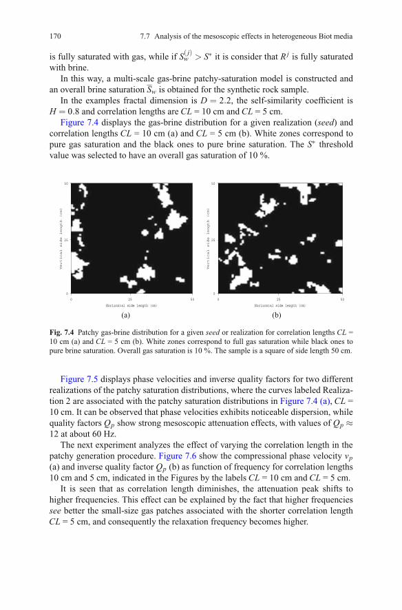
170
is fully saturated with gas, while if S( j)w > S∗ it is consider that Rj is fully saturatedwith brine.
In this way, a multi-scale gas-brine patchy-saturation model is constructed andan overall brine saturation Sw is obtained for the synthetic rock sample.
In the examples fractal dimension is D = 2.2, the self-similarity coefficient isH = 0.8 and correlation lengths are CL = 10 cm and CL = 5 cm.
Figure 7.4 displays the gas-brine distribution for a given realization (seed) andcorrelation lengths CL = 10 cm (a) and CL = 5 cm (b). White zones correspond topure gas saturation and the black ones to pure brine saturation. The S∗ thresholdvalue was selected to have an overall gas saturation of 10 %.
0
25
50
0 25 50
Vertical side length (cm)
Horizontal side length (cm)
0
25
50
0 25 50
Vertical side length (cm)
Horizontal side length (cm)
(a) (b)
Fig. 7.4 Patchy gas-brine distribution for a given seed or realization for correlation lengths CL =10 cm (a) and CL = 5 cm (b). White zones correspond to full gas saturation while black ones topure brine saturation. Overall gas saturation is 10 %. The sample is a square of side length 50 cm.
Figure 7.5 displays phase velocities and inverse quality factors for two differentrealizations of the patchy saturation distributions, where the curves labeled Realiza-tion 2 are associated with the patchy saturation distributions in Figure 7.4 (a), CL =10 cm. It can be observed that phase velocities exhibits noticeable dispersion, whilequality factors Qp show strong mesoscopic attenuation effects, with values of Qp ≈12 at about 60 Hz.
The next experiment analyzes the effect of varying the correlation length in thepatchy generation procedure. Figure 7.6 show the compressional phase velocity vp(a) and inverse quality factor Qp (b) as function of frequency for correlation lengths10 cm and 5 cm, indicated in the Figures by the labels CL = 10 cm and CL = 5 cm.
It is seen that as correlation length diminishes, the attenuation peak shifts tohigher frequencies. This effect can be explained by the fact that higher frequenciessee better the small-size gas patches associated with the shorter correlation lengthCL = 5 cm, and consequently the relaxation frequency becomes higher.
7.7 Analysis of the mesoscopic effects in heterogeneous Biot media

171
1 10 100Frequency (Hz)
2.4
2.5
2.6
2.7
Vp
(km
/s)
Realization 1Realization 2
1 10 100Frequency (Hz)
0
0.02
0.04
0.06
0.08
1/Q
p
Realization 1Realization 2
(a) (b)
On the other hand, compressional phase velocities in Figure 7.6 are not sensitiveto this change in correlation length at low frequencies, while at higher frequenciesthe differences are small, the order of 1.4 %.
1 10 100Frequency (Hz)
2.4
2.5
2.6
2.7
Vp
(km
/s)
CL = 10 cmCL = 5cm
1 10 100Frequency (Hz)
0
0.02
0.04
0.06
0.08
1/Q
p
CL = 10 cmCL = 5 cm
(a) (b)
Fig. 7.6 Compressional phase velocity vp (a) and inverse quality factor Qp (b) obtained from thecompressibility test for correlation lengths CL equal to 10 cm and 5 cm. Overall CO2 saturation is10 %.
Figures 7.7 and 7.8 show the absolute value of the the fluid pressure distributionat frequencies 10 Hz and 65 Hz, respectively, for the patchy distribution realizationin Figure 7.4(a) with correlation length CL = 10 cm.
It can be observed that pressure gradients take their highest values at the brine-gas contact interfaces, with higher values at 65 Hz than at 10 Hz. This correspondsto the higher mesoscopic attenuation values at 65 Hz as compared with those at 10Hz observed in the black curve in Figure 7.6(b).
Fig. 7.5 P-wave phase velocity vp (a) and inverse quality factor Qp (b) obtained from the com-pressibility test for 2 seeds or realizations of the patchy saturation model. Overall gas saturationis 10 %.
7 Modeling Biot media at the meso-scale using a finite element approach

172
0
25
50Vertical side length (cm)
Horizontal side length (cm) 0
0.02
0.04
0.06
0.08
0.1
0.12
0.14
Fluid Pressure (Pa)
Fig. 7.7 Absolute value of fluid pressure distribution (Pa) at 10 Hz and 10 % CO2 gas saturation.The sample is a square of side length 50 cm. Correlation length is CL = 10 cm.
0
25
50
Vertical side length (cm)
Horizontal side length (cm) 0
0.05
0.1
0.15
0.2
0.25
0.3
0.35
Fluid Pressure (Pa)
Fig. 7.8 Absolute value of fluid pressure distribution (Pa) at 65 Hz and 10 % CO2 gas saturation.The sample is a square of side length 50 cm. Correlation length is CL = 10 cm.
7.7 Analysis of the mesoscopic effects in heterogeneous Biot media

173
7.7.2 The case of a porous matrix composed of a shale-sandstonequasi-fractal mixture
The finite element procedures (7.17) and (7.18) were implemented to analyze theresponse of a brine saturated rock sample with the solid matrix composed of twodifferent materials: shale and the sandstone 2 of Table 1. The domain Ω is a squareof side length 5 cm, and the partition T h is composed of 75×75 squares Rj, so thatΩ = ∪J
j=1Rj.
We assume a distribution of shale and sandstone in the form of irregular patchesusing an stochastic fractal field based on the von Karman spectrum in (7.21).
The procedure to generate this rock sample is similar to that explained for thecase of patchy saturation. We assign to each sub-domain Rj a pseudo-random num-ber using a generator with uniform distribution. This random field is Fourier trans-formed to the spatial wave-number domain and its amplitude spectrum is multi-plied by the spectrum given in equation (7.21). The result is then transformed backto the spatial domain, obtaining a micro-heterogeneous sandstone content modelS( j), j = 1, · · · ,J.
Next, to assign to the porous solid matrix in each Rj pure shale or pure sandstone,we choose a threshold value S∗ so that for each sub-domain Rj where S( j) ≤ S∗ weassume that such sub-domain matrix is pure shale, while if S( j) > S∗ we considerthat Rj is pure sandstone.
In this way, a multi-scale highly-heterogeneous quasi-fractal model is con-structed and an overall sandstone content S is obtained for the synthetic rock sample.In this experiment we choose S∗ so that the overall sandstone content S is equal to50 %.
We generated two realizations of the model for two different correlation lengths,labeled as CL = 0.0025 cm and CL = 0.05 cm in the figures. The other parametersof the fractal spectrum density are self-similarity coefficient H = 0.8 and fractaldimension D= 2.2.
The distribution of shale and sandstone obtained in this fashion for the case ofcorrelation length CL = 0.05 cm is illustrated in Figure 7.9, where the black zonescorrespond to pure shale while the white ones to pure sandstone.
These mesoscopic-scale heterogeneities produce non-negligible mesoscopic at-tenuation effects as shown in Figure 7.10(b) for both correlation lengths. It can beobserved values of Qs of about 75 for frequencies between 20 and 40 Hz for bothcorrelation lengths. The attenuation peak moves to higher frequencies for the caseof the shorter correlation length. On the other hand, the shear phase velocity in Fig-ure 7.10(a) shows very slight dispersion, with a 1.5 % increase between 0.3 and 100Hz.
This mesoscopic attenuation effects are visualized in Figure 7.11 displaying theabsolute value of the fluid pressure. As in the case of patchy saturation, the pressuregradients at the boundaries of the heterogeneities illustrate the induced fluid flowmechanism.
7 Modeling Biot media at the meso-scale using a finite element approach
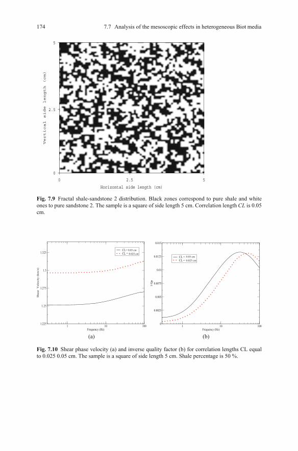
174
0
2.5
5
0 2.5 5
Vertical side length (cm)
Horizontal side length (cm)
Fig. 7.9 Fractal shale-sandstone 2 distribution. Black zones correspond to pure shale and whiteones to pure sandstone 2. The sample is a square of side length 5 cm. Correlation lengthCL is 0.05cm.
1 10 100Frequency (Hz)
1.225
1.25
1.275
1.3
1.325
Shea
r V
eloci
ty (
km
/s)
CL= 0.025 cm CL = 0.05 cm0.025 cm
0.05 cm
1 10 100Frequency (Hz)
0
0.0025
0.005
0.0075
0.01
0.0125
0.015
1/Q
p
CL = 0.025 cmCL = 0.05 cm
0.05 cm0.025 cm
(a) (b)
Fig. 7.10 Shear phase velocity (a) and inverse quality factor (b) for correlation lengths CL equalto 0.025 0.05 cm. The sample is a square of side length 5 cm. Shale percentage is 50 %.
7.7 Analysis of the mesoscopic effects in heterogeneous Biot media

175
0
25
50Vertical side length (cm)
Horizontal side length (cm) 0
0.1
0.2
0.3
0.4
0.5
0.6
0.7
0.8
0.9
Lame Coefficient lambda (Pa)
Fig. 7.11 Absolute fluid pressure distribution (Pa) at 30 Hz. Correlation lengths CL is 0.05 cm.The sample is a square of side length 5 cm. Shale percentage is 50 %.
These lithological variations also induce wave-induce fluid flow and mesoscopicloss effects in the case of the compressibility tests in the p33-experiment. These ef-fects are shown in Figure 7.12, with values of the quality factor Qp of compressionalwaves of about 70 at 65 Hz. The corresponding compressional phase velocity showsvery slight dispersion, with an increase of 1.7 % between 0.1 and 100 Hz. The figureis not included for brevity.
This result demonstrates that fast shear and compressional waves propagatingthrough Biot media with heterogeneities in the solid matrix are also affected bywave-induce fluid flow effects.
7.8 Application of the Montecarlo approach to determine meanphase velocities and quality factors in Biot media with fractalheterogeneity distributions. The patchy gas-brine case
As mentioned in the Introduction to this Chapter, a precise knowledge of the spa-tial distribution of the rock heterogeneities at mesoscopic scales is in general notavalaible. Instead, averages and variances of the material properties may be known.
7 Modeling Biot media at the meso-scale using a finite element approach

176
Fig. 7.12 Shear inverse qual-ity factors Qs and Qp forcorrelation lengths is CL =0.05 cm. The sample is asquare of side length 5 cm.Shale percentage is 50 %.
1 10 100Frequency (Hz)
0
0.005
0.01
0.015
1/Q
1/Qs, CL = 0.051/Qp, CL = 0.05 cm
This fact suggest to represent the heterogeneities as stochastic functions withgiven spectral density distributions. This approach was used in [Helle et al., 2003]using the von Karman self-similar correlation spectral density in (7.21) to modelpatchy fluid distributions. Also, [Masson and Pride, 2007] analyzed the behaviourof materials with local properties randomly sampled from certain probability distri-butions.
Here the application of the Montecarlo procedure is illustrated for the case ofpatchy gas-brine saturation.
A set of seventy experiments was performed, each one associated with a realiza-tion of a patchy gas-brine distribution. For all realizations S∗ was chosen so that theoverall gas saturation was 10%. The correlation length CL in (7.21) was taken to be10 cm and frequency was varied from 0.3 to 100 Hz. Figure 7.4(a) shows one of the70 realizations used in the Montecarlo procedure.
To stop the Montecarlo simulations the stabilization of the variance of the com-puted variables was analyzed. Figure 7.13 shows the variance of the compressionalphase velocity vp averaged in the whole range of frequencies as a function of thenumber of realizations. It can be observed that after 70 realizations the variance sta-bilizes at an almost constant value. A a similar behaviour observed for the inversequality factor; the corresponding figure is not included.
This fact allows us to define the mean compressional velocity vp and mean com-pressional inverse quality factor 1/Qp as the effective compressional velocity andinverse quality factor of a viscoelastic medium equivalent to this type of Biot media.
Figure 7.14 displays the mean compressional velocity vp and inverse quality fac-tor Qp versus frequency after 70 realizations and their corresponding standard devi-ation (indicated with dotted lines). It can be observed a noticeable dispersion of thecompressional phase velocity in the whole frequency range. Besides, mesoscopic at-tenuation is very important for almost all the frequency range under consideration,with a value of Qp = 12 at about 20 Hz. This shows the high amplitude losses thatsuffer the fast compressional waves travelling through these kind of Biot media.
7.8 Application of the Montecarlo approach to determine mean phase velocities...

177
Fig. 7.13 Average variance ofcompressional phase velocityas a function of the totalnumber of realizations.
0
0.0005
0.001
0.0015
0.002
0.0025
0.003
0.0035
0.004
0 10 20 30 40 50 60 70
Ave
rage
Vp
vari
ance
(K
m2 /s
2 )Total number of realizations
2.4
2.45
2.5
2.55
2.6
2.65
2.7
0.1 1 10 100
Vp
(Km
/s)
Frequency (Hz)
0
0.01
0.02
0.03
0.04
0.05
0.06
0.07
0.08
0.09
0.1
0.1 1 10 100
1/Q
p
Frequency (Hz)
(a) (b)
Fig. 7.14 Average equivalent compressional phase velocity vp ((a), solid line) and inverse qualityfactor Qp ((b), solid line) as function of frequency. Dotted lines indicate its corresponding standarddeviation interval.
Note also the lack of uncertainty at low frequencies, as expected from a viscoelastic-type material ([Ferry, 1970]), since for long wavelengths the medium is seen ashomogeneous independently of the realization. As frequency increases, the shorterwavelengths start to see the differences among realizations, with the increasing vari-ances observed in Figure 7.14.
The effective shear modulus of this sample was checked to coincide numericallywith the the shear modulus of the dry matrix. This happens because shear tests ap-plied on samples with fluid heterogeneities like patchy gas-brine saturation, inducenegligible fluid-pressure gradients and, consequently, negligible mesoscopic effects.
7 Modeling Biot media at the meso-scale using a finite element approach
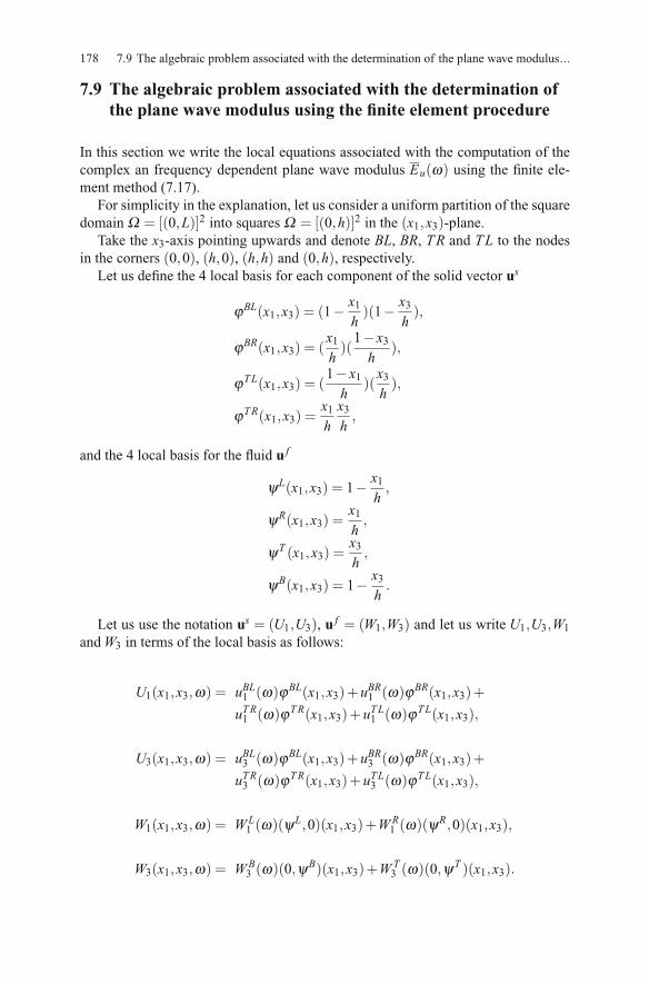
178
7.9 The algebraic problem associated with the determination ofthe plane wave modulus using the finite element procedure
In this section we write the local equations associated with the computation of thecomplex an frequency dependent plane wave modulus Eu(ω) using the finite ele-ment method (7.17).
For simplicity in the explanation, let us consider a uniform partition of the squaredomain Ω = [(0,L)]2 into squares Ω = [(0,h)]2 in the (x1,x3)-plane.
Take the x3-axis pointing upwards and denote BL, BR, TR and TL to the nodesin the corners (0,0), (h,0), (h,h) and (0,h), respectively.
Let us define the 4 local basis for each component of the solid vector us
ϕBL(x1,x3) = (1− x1
h)(1− x3
h),
ϕBR(x1,x3) = (x1
h)(
1− x3
h),
ϕTL(x1,x3) = (1− x1
h)(x3
h),
ϕTR(x1,x3) =x1
hx3
h,
and the 4 local basis for the fluid u f
ψL(x1,x3) = 1− x1
h,
ψR(x1,x3) =x1
h,
ψT (x1,x3) =x3
h,
ψB(x1,x3) = 1− x3
h.
Let us use the notation us = (U1,U3), u f = (W1,W3) and let us write U1,U3,W1
and W3 in terms of the local basis as follows:
U1(x1,x3,ω) = uBL1 (ω)ϕBL(x1,x3)+uBR1 (ω)ϕBR(x1,x3)+
uTR1 (ω)ϕTR(x1,x3)+uTL1 (ω)ϕTL(x1,x3),
U3(x1,x3,ω) = uBL3 (ω)ϕBL(x1,x3)+uBR3 (ω)ϕBR(x1,x3)+
uTR3 (ω)ϕTR(x1,x3)+uTL3 (ω)ϕTL(x1,x3),
W1(x1,x3,ω) = WL1 (ω)(ψL,0)(x1,x3)+WR
1 (ω)(ψR,0)(x1,x3),
W3(x1,x3,ω) = WB3 (ω)(0,ψB)(x1,x3)+WT
3 (ω)(0,ψT )(x1,x3).
7.9 The algebraic problem associated with the determination of the plane wave modulus...

179
The coefficients
uBL1 (ω),uBR1 (ω),uTR1 (ω),uTL1 (ω),
uBL3 (ω),uBR3 (ω),uTR3 (ω),uTL3 (ω),
WL1 (ω),WR
1 (ω),WB3 (ω),WT
3 (ω)
are the 12 unknowns in the 12×12 linear system to be defined next.First note that the weak form (7.17) can be written in the form
Λ(u,v) = iω(η κ−1u f ,v f )+(λu∇ ·us,∇ ·vs)+2(με11(us),ε11(vs))
+2(με33(us),ε33(vs))+4(με13(us),ε13(vs))
+(B ∇ ·u f ,∇ ·vs)+(B ∇ ·us,∇ ·v f )+(M ∇ ·u f ,∇ ·v f )
=−〈ΔP,vs ·ν〉Γ T , ∀ v ∈ V(h,p). (7.23)
Also,
ε11((ϕBL(x1,x3),0)) =∂ϕBL(x1,x3)
∂x1,
ε13((ϕBL(x1,x3),0)) =12
∂ϕBL(x1,x3)
∂x3,
ε33((ϕBL(x1,x3),0)) = 0,
∇ · ((ϕBL(x1,x3),0)) =∂ϕBL(x1,x3)
∂x1.
To get the equation for the first unknown uBL1 , choose vs=(vs1,vs3)=(ϕBL(x1,x3),0)
and v f = (0,0) in (7.23) to get the equation
[((λu+2μ)
∂ϕBL
∂x1,
∂ϕBL
∂x1
)+
(μ
∂ϕBL
∂x3,
∂ϕBL
∂x3
)]uBL1
+
[((λu+2μ)
∂ϕBR
∂x1,
∂ϕBL
∂x1
)+
(μ
∂ϕBR
∂x3,
∂ϕBL
∂x3
)]uBR1
+
[((λu+2μ)
∂ϕTR
∂x1,
∂ϕBL
∂x1
)+
(μ
∂ϕTR
∂x3,
∂ϕBL
∂x3
)]uTR1
+
[((λu+2μ)
∂ϕTL
∂x1,
∂ϕBL
∂x1
)+
(μ
∂ϕTL
∂x3,
∂ϕBL
∂x3
)]uTL1
+
[(λu
∂ϕBL
∂x3,
∂ϕBL
∂x1
)+
(μ
∂ϕBL
∂x1,
∂ϕBL
∂x3
)]uBL3 (7.24)
+
[(λu
∂ϕBR
∂x3,
∂ϕBL
∂x1
)+
(μ
∂ϕBR
∂x1,
∂ϕBL
∂x3
)]uBR3
7 Modeling Biot media at the meso-scale using a finite element approach

180
+
[(λu
∂ϕTR
∂x3,
∂ϕBL
∂x1
)+
(μ
∂ϕTR
∂x1,
∂ϕBL
∂x3
)]uTR3
+
[(λu
∂ϕTL
∂x3,
∂ϕBL
∂x1
)+
(μ
∂ϕTL
∂x1,
∂ϕBL
∂x3
)]uTL3
+
[(B
∂ψL
∂x1,
∂ϕBL
∂x1
)]WL
1 +
[(B
ψR
∂x1,
∂ϕBL
∂x1
)]WR
1
+
[(B
∂ψB
∂x3,
∂ϕBL
∂x1
)]WB
3 +
[(B
∂ψT
∂x3,
∂ϕBL
∂x1
)]WT
3
≡ a11uBL1 +a12u
BR1 +a13u
TR1 +a14u
TL1 +a15u
BL3 +a16u
TR3 +a17u
TR3 +a18u
TL3
+a19WL1 +a1,10W
R1 +a1,11W
B3 +a1,12W
T3 =−⟨ΔP,(ϕBL(x1,x3),0) ·ν
⟩Γ T = 0.
nent of (ϕBL(x1,x3),0) on the top boundary vanishes.In (7.24) the unknowns are numbered in the form:
1 → uBL1 , 2 → uBR1 , 3 → uTR1 , 4 → uTL1 ,
5 → uBL3 , 6 → uBR3 , 7 → uTR3 , 8 → uTL3 ,
9 →WL1 , 10 →WR
1 , 11 →WB3 , 12 →WT
3 .
Next, taking the test functions vs = (ϕBR,0),vs = (ϕTR,0),vs = (ϕTL,0),v f =(0,0) in (7.23) we get three equations similar to (7.24) changing the function ϕBL
appearing before the right parenthesis in all inner products in (7.24) by ϕBR,ϕTR
and ϕTL, respectively.To get the fifth equation for the unknown uBL3 take the test function vs =
(0,ϕBL(x1,x3)) = (vs1,vs3),v
f = (0,0) in (7.23) and note that
ε33((0,ϕBL(x1,x3))) =∂ϕBL(x1,x3)
∂x3,
ε13((0,ϕBL(x1,x3))) =12
∂ϕBL(x1,x3)
∂x1,
ε1((0,ϕBL(x1,x3))) = 0,
∇ · (0,ϕBL(x1,x3)) =∂ϕBL(x1,x3)
∂x3.
Then the following equation is obtained:[(λu
∂ϕBL
∂x1,
∂ϕBL
∂x3
)+
(μ
∂ϕBL
∂x3,
∂ϕBL
∂x1
)]uBL1 (7.25)
7.9 The algebraic problem associated with the determination of the plane wave modulus...
Remark. In this equation the right-hand side vanishes since the normal compo-

181
+
[(λu
∂ϕBR
∂x1,
∂ϕBL
∂x3
)+
(μ
∂ϕBR
∂x3,
∂ϕBL
∂x1
)]uBR1
+
[(λu
∂ϕTR
∂x1,
∂ϕBL
∂x3
)+
(μ
∂ϕTR
∂x3,
∂ϕBL
∂x1
)]uTR1
+
[(λu
∂ϕTL
∂x1,
∂ϕBL
∂x3
)+
(μ
∂ϕTL
∂x3,
∂ϕBL
∂x1
)]uTL1
+
[((λu+2μ)
∂ϕBL
∂x3,
∂ϕBL
∂x3
)+
(μ
∂ϕBL
∂x1,
∂ϕBL
∂x1
)]uBL3
+
[((λu+2μ)
∂ϕBR
∂x3,
∂ϕBL
∂x3
)+
(μ
∂ϕBR
∂x1,
∂ϕBL
∂x1
)]uBR3
+
[((λu+2μ)
∂ϕTR
∂x3,
∂ϕBL
∂x3
)+
(μ
∂ϕTR
∂x1,
∂ϕBL
∂x1
)]uTR3
+
[((λu+2μ)
∂ϕTL
∂x3,
∂ϕBL
∂x3
)+
(μ
∂ϕTL
∂x1,
∂ϕBL
∂x1
)]uTL3
+
[(B
∂ψL
∂x1,
∂ϕBL
∂x3
)]WL
1 +
[(B
∂ψR
∂x1,
∂ϕBL
∂x3
)]WR
1
+
[(B
∂ψB
∂x3,
∂ϕBL
∂x3
)]WB
3 +
[(B
∂ψT
∂x3,
∂ϕBL
∂x3
)]WT
3
≡ a51uBL1 +a52u
BR1 +a53u
TR1 +a54u
TL1 +a55u
BL3 +a56u
TR3 +a57u
TR3 +a58u
TL3
+a5,9WL1 +a5,10W
R1 +a5,11W
B3 +a5,12W
T3 = 0,
Next, taking the test functions vs = (0,ϕBR(x1,x3)),vs = (0,ϕTR(x1,x3)),vs =(0,ϕTL(x1,x3)),v f = (0,0) in (7.23) we get the sixth, seventh and eighth equationswith coefficients a6 j,a7 j,a8 j, j= 1, · · · ,12, defined similarly than those in (7.25), re-placing the function ϕBL appearing before the right parenthesis in all inner productsin (7.25) by ϕBR,ϕTR and ϕTL, respectively.
Next take the test function vs = (0,0),v f = (ψL(x1,x3),0) in (7.23) and note that
ε33(vs) = ε13(vs) = ε11(vs) = 0, ∇ · (ψL,0) =∂ψL(x1,x3)
∂x1
to get the 9th equation:[(B
∂ϕBL
∂x1,
∂ψL
∂x1
)]uBL1 +
[(B
∂ϕBR
∂x1,
∂ψL
∂x1
)]uBR1
+
[(B
∂ϕTR
∂x1,
∂ψL
∂x1
)]uTR1 +
[(B
∂ϕTL
∂x1,
∂ψL
∂x1
)]uTL1
+
[(B
∂ϕBL
∂x3,
∂ψL
∂x1
)]uBL3 +
[(B
∂ϕBR
∂x3,
∂ψL
∂x1
)]uBR3 (7.26)
7 Modeling Biot media at the meso-scale using a finite element approach

182
+
[(B
∂ϕTR
∂x3,
∂ψL
∂x1
)]uTR3 +
[(B
∂ϕTL
∂x3,
∂ψL
∂x1
)]uTL3
+
[iω(η κ−1ψL,ψL)+(M ∂ψL
∂x1,
∂ψL
∂x1
)]WL
1
+
[iω(η κ−1ψR,ψL)+((M ∂ψR
∂x1,
∂ψL
∂x1
)]WR
1
+
(M
∂ψB
∂x3,
∂ψL
∂x1
)WB
3 +
(M
∂ψT
∂x3,
∂ψL
∂x1
)WT
3
≡ a91uBL1 +a92u
BR1 +a93u
TR1 +a94u
TL1 +a95u
BL3 +a96u
TR3 +a97u
TR3 +a98u
TL3
+a99WL1 +a9,10W
R1 +a9,11W
B3 +a9,12W
T3 = 0.
Taking the the test functions vs = (0,0),v f = (ψR(x1,x3),0) in (7.23) to get thethe 10th- equation replacing ψL by ψR in all inner products appearing before theright parenthesis in (7.26).
Next take the test function vs = (0,0),v f = (0,ψB(x1,x3)) in (7.23) and note that
ε33(vs) = ε13(vs) = ε11(vs) = 0, ∇ · (0,ψB) =∂ψB(x1,x3)
∂x3
to get the 11th equation:
+
[(B
∂ϕBL
∂x1,
∂ψB
∂x3
)]uBL1 +
[(B
∂ϕBR
∂x1,
∂ψB
∂x3
)]uBR1
+
[(B
∂ϕTR
∂x1,
∂ψB
∂x3
)]uTR1 +
[(B
∂ϕTL
∂x1,
∂ψB
∂x3
)]uTL1
+
[(B
∂ϕBL
∂x3,
∂ψB
∂x3
)]uBL3
+
[(B
∂ϕBR
∂x3,
∂ψB
∂x3
)]uBR3 +
[(B
∂ϕTR
∂x3,
∂ψB
∂x3
)]uTR3 (7.27)
+
[(B
∂ϕTL
∂x3,
∂ψB
∂x3
)]uTL3
+
(M
∂ψL
∂x1,
∂ψB
∂x3
)WL
1 +
(M
∂ψR
∂x1,
∂ψB
∂x3
)WR
1
+
[iω(η κ−1ψB,ψB)+(M ∂ψB
∂x3,
∂ψB
∂x3
)]WB
3
+
[iω(η κ−1ψT ,ψB)+((M ∂ψT
∂x3,
∂ψB
∂x3
)]WT
3
≡ a11,1uBL1 +a11,2u
BR1 +a11,3u
TR1 +a11,4u
TL1 +a11,5u
BL3 +a11,6u
TR3 +a11,7u
TR3 +a11,8u
TL3
+a11,9WL1 +a11,10W
R1 +a11,11W
B3 +a11,12W
T3 = 0.
7.9 The algebraic problem associated with the determination of the plane wave modulus...

183
Finally, take the test function vs = (0,0),v f = (0,ψT (x1,x3)) in (7.23) and re-place ψB by ψT in all inner products appearing before the right parenthesis in (7.27)to get the 12th equation.
right-hand side of (7.23) when the element has the top face contained in the topboundary Γ T of the sample Ω .
All inner products in the twelve equations above were computed assuming con-stant coefficients on each computational cell.
Next, the assembly of the global matrix can be performed using a global num-bering connectivity matrix as usually done when constructing the global matrix ofthe linear system in any finite element code (see for example [Becker et al., 1981]).
7.10 Appendix 1. Uniqueness of the solution of the variationalproblems
The boundary-value problems formulated in this Chapter are associated with second-order operators having boundary data in L2(Ω). Existence will be assumed for thesolution of these problems. Also, following [Dahlberg et al., 1988] we will assumethat u(s,P),u(s,T ) ∈ [H3/2]2; we refer to [Adams, 1975] for the definition of Sobolevspaces Hs(Ω) for s any real number.
On the other hand, it will be assumed that u( f ,P),u( f ,T ) ∈ H1(div;Ω). These as-sumptions will be used in the proof of the theorem stated below.
Theorem 7.3. Assume that u(s,P),u(s,T ) ∈ [H3/2(Ω)]2,u( f )f ∈ H1(div;Ω). Also as-sume that the coefficients in the constitutive relations (7.1)-(7.2) satisfy the condi-tions stated in (1.58), so that the matrix D in (7.15) is positive definite. Then for anyω > 0 the solution of problems (7.13) and (7.16) is unique.
Proof: To analyze the uniqueness of the solution of (7.13), set ΔP = 0 and choosev= u(P) in (7.13) to obtain the equation
iω(
ηκ−1u( f ,P),u( f ,P))+(D ε(u(P)), e(u(P))
)= 0. (7.28)
Choose the imaginary part in (7.28) to conclude that
‖u( f ,P)‖0 = 0. (7.29)
Using (7.29) in (7.28) we obtain
(D e(u(s,P)), e(u(s,P))
)= 0, (7.30)
where
TR), and (0,ϕTL) will contribute to theRemark. Only the test functions (0,ϕ
7 Modeling Biot media at the meso-scale using a finite element approach

184
D=
⎛⎝λu+2μ λu 0λu λu+2μ 00 0 4μ
⎞⎠ ,
e(u(s,P)) =
⎛⎝ ε11(u(s,P))ε33(u(s,P))ε13(u(s,P))
⎞⎠ .
Next, since the matrix D in (7.15) is positive definite, so it is the matrix D, whichfrom (7.30) allow us to conclude that
‖ε11(u(s,P))‖0 = ‖ε33(u(s,P))‖0 = ‖ε13(u(s,P))‖0 = 0. (7.31)
Thus, using that functions vanishing in L2(Ω) vanish almost everywhere in Ω (in-dicated as a.e. in Ω , i.e. vanish in Ω up to a set of measure zero) [Adams, 1975], wehave
ε11(u(s,P)) =∂u(s,P)1 (x1,x3)
∂x1= 0, ε33(u(s,P)) =
∂u(s,P)3 (x1,x3)
∂x3= 0, a.e. inΩ,
so that
u(s,P)1 (x1,x3) = f (x3), u(s,P)3 (x1,x3) = g(x1) a.e. in Ω. (7.32)
Hence from (7.31) and (7.32) we have
2 ε13(u(s,P)) =∂ f (x3)
∂x3+
∂g(x1)
∂x1= 0, a.e. in Ω,
which in turn implies
∂ f (x3)
∂x3=−∂g(x1)
∂x1=C = constant a.e. in Ω.
Hence,
g(x1) =−Cx1 +A, f (x3) =Cx3 +B, a.e. in Ω.
Now by the Sobolev embedding [Adams, 1975]
H3/2(Ω)→C0(Ω)
so that u(s,P)1 ,u(s,P)3 are uniformly continuous functions on Ω . Consequently (7.32)
holds for all (x1,x3) ∈ Ω as uniformly continuous functions, and u(s,P)1 ,u(s,P)3 haveunique extensions to ∂Ω . Hence,
7.10 Appendix 1. Uniqueness of the solution of the variational problems
185
u(s,P)1 (x1,x3) = f (x3), u(s,P)3 (x1,x3) = g(x1) ∀ (x1,x3) ∈ Ω . (7.33)
On the other hand, the boundary condition (7.7) tells us that the normal compo-nents of the traces of u(s,P) vanish on Γ B∪Γ L, so that
u(s,P)1 (0,x3) = 0, u(s,P)3 (x1,0) = 0. (7.34)
Thus (7.33) and (7.34) imply that
u(s,P)1 (x1,x3) = u(s,P)3 (x1,x3) = 0, (x1,x3) ∈ Ω
and we have uniqueness for the solution of (7.13).Let us analyze uniqueness for the solution of (7.16). Set ΔT = 0 and choose
v = u(T ) in (7.16). Repeating the argument given to show uniqueness for u(s,P) weobtain
‖u( f ,T )‖0 = 0, (7.35)
‖ε11(u(s,T ))‖0 = ‖ε33(u(s,T ))‖0 = ‖e13(u(s,T ))‖0 = 0.
Next, note that since elements in V T (Ω) vanish on Γ B (see (7.11))
‖|v‖|=(
∑k,l
∫Ω|εkl(v)|2dΩ
)1/2
defines a norm on V T (Ω) equivalent to the H1-norm in Ω , [Ciarlet, 1976]. Thusfrom (7.35) we see that
‖u(s,T )‖1 = 0. (7.36)
From (7.35) and (7.36) we see that uniqueness holds for the solution of (7.16). Thiscompletes the proof.
7.11 Appendix 2. Calculation of the complex plane wave modulusin a periodic system of fluid-saturated porous layers
We consider a periodic layered system composed of porous media 1 and 2 withthickness dl , l = 1,2 and period d1 + d2. [White et al., 1975] obtained the complexmodulus for a P1-wave travelling along the direction perpendicular to the stratifica-tion. The result, summarized in [Carcione and Picotti, 2006] is given by
E =
[1E0
+2(r2 − r1)
2
iω(d1 +d2)(I1 + I2)
]−1
,
7 Modeling Biot media at the meso-scale using a finite element approach
186
where
E0 =
(p1
Eu1
+p2
Eu2
)−1
, (7.37)
is the Reuss average, with pl = dl/(d1 + d2), l = 1,2. Omitting the subindex l forclarity, we have for each medium
Eu = Ku+43
μ , (7.38)
where Ku is the undrained or closed bulk modulus given by equation (1.51).Moreover,
r =α MEu
is the ratio of fast P-wave fluid tension to total normal stress, with M is given by(1.50). Besides
I =η κ−1
kcoth
(kd2
)is an impedance related to the slow P wave,
k =
√iωη κ−1
KE(7.39)
is the complex wave-number of the slow P wave, and
KE =EmMEu
,
is an effective modulus, with
Em = Km+43
μ
the dry-rock fast P-wave modulus.Let us assume in the following analysis that the properties of the frame are the
same in media 1 and 2 and that the contrast is due to two different saturating fluids(for example, water and gas). The approximate transition frequency separating therelaxed and unrelaxed states (i.e., the approximate location of the relaxation peakindicating flow or no-flow, respectively) is
fm =8κ1KE1
πη1d21, (7.40)
where the subindex 1 refers to water for a layered medium alternately saturatedwith water and gas. At this reference frequency, the Biot slow-wavelength equals themean layer thickness or characteristic length of the inhomogeneities [Gurevich et al.,1997].
7.11 Appendix 2. Calculation of the complex plane wave modulus in a periodic system...

187
Equation (7.40) indicates that the mesoscopic-loss mechanism moves towardsthe low frequencies with increasing viscosity and decreasing permeability, i.e., theopposite behaviour of the Biot relaxation mechanism.
The mesoscopic mechanism is due to the presence of the Biot slow wave and thediffusivity constant is
γ = κKE/η .
The critical fluid-diffusion relaxation length Lr is obtained by setting |kLr| = 1,where k is the wave-number (7.39). It gives
Lr =√
γ/ω.
The fluid pressures will be equilibrated if Lr is comparable to the period of thestratification. For smaller diffusion lengths (e.g., higher frequencies) the pressureswill not be equilibrated, causing attenuation and velocity dispersion. Notice that thereference frequency (7.40) is obtained for a diffusion length Lr = d1/4.
At enough low frequencies, the fluid pressure is uniform (iso-stress state) and theeffective modulus of the pore fluid is given by Wood’s law [Wood, 1955]:
1Kf
=p1
Kf1+
p2
Kf2. (7.41)
It can be shown [Johnson, 2001] that E(ω = 0) is equal to the plane-wave modulus(7.38) for a fluid whose composite modulus is given by Wood’s law in equation(7.41).
On the other hand, at high frequencies, the pressure is not uniform but canbe assumed to be constant within each phase. In such a situation Hill’s theorem[Hill, 1964] gives the high-frequency limit E(ω = ∞) = E0 with E0 given in equa-tion (7.37).
7 Modeling Biot media at the meso-scale using a finite element approach

Chapter 8
The meso-scale. Fractures as thin layers in Biotmedia and induced anisotropy
Abstract A fluid-saturated poroelastic isotropic medium with aligned fractures be-haves as a transversely isotropic and viscoelastic (TIV) medium when the predom-inant wavelength is much larger than the average distance between fractures. Herefractures are modeled as extremely thin and compliant porous layers. P-waves trav-elling in this type of medium generate fluid flow and slow (diffusion) Biot waves,causing attenuation and dispersion of the fast modes (mesoscopic loss). This chap-ter presents a set of compressibility and shear time-harmonic experiments on highlyheterogeneous fractured poroelastic samples to determine the five complex and fre-quency dependent stiffnesses characterizing the equivalent TIV medium. These ex-periments are identified with boundary-value problems which solutions are com-puted using finite element procedures.
8.1 Introduction
Fractured hydrocarbon reservoirs have been the subject of interest in exploration andproduction geophysics, since generally, natural fractures control the permeabilityof the reservoir [Gurevich et al., 2009]. In geophysical prospecting and reservoirdevelopment, knowledge of orientation, densities and sizes of fractures is essentialsince these factors control hydrocarbon production [Gurevich, 2003].
This knowledge and analysis is also important in the monitoring of injectedplumes of CO2 in geological storage. There might be faults and fractures that canleak CO2 to the surface [Picotti et al., 2012].
One of the important mechanisms of seismic attenuation in fluid-saturated porousmedia is wave-induced fluid flow, by which the fast compressional and shear wavesare converted to slow (diffusive) Biot waves at mesoscopic-scale heterogeneities,which are larger than the pore size but much smaller than the predominant wave-lengths of the fast compressional and shear waves [Carcione and Picotti, 2006,Carcione, 2014]. These effects were analyzed in detail in Chapter 7.
© Springer International Publishing AG 2016
in Geosystems Mathematics and Computing, DOI 10.1007/978-3-319-48457-0_8
189J.E. Santos, P.M. Gauzellino, Numerical Simulation in Applied Geophysics, Lecture Notes

190
White et al. [White et al., 1975, White, 1975] were the first to introduce themesoscopic-loss mechanism in the framework of Biot theory considering alternat-ing thin poroelastic layers with symmetry axes perpendicular to the layering plane[Carcione and Picotti, 2006]. Gelinsky and Shapiro [Gelinsky and Shapiro, 1997]obtained the relaxed and unrelaxed (real) stiffnesses of the equivalent poro-viscoelasticmedium to a finely layered horizontally homogeneous material.
Krzikalla and Muller [Krzikalla and Muller, 2011] combined the previous mod-els to obtain the five complex and frequency-dependent stiffnesses of the equivalenttransversely isotropic viscoelastic (TIV) medium. Their approach assumes a 1-Dcharacter of the fluid pressure equilibration process which generates diffusive modesfrom the fast compressional wave, i.e., the fluid-flow direction is perpendicular tothe fracture layering. As a consequence, compressional waves travelling horizon-tally or vertically or shear waves will generate fluid pressure in such a way as tomaintain its distribution. Thus, the model considers only one relaxation function,corresponding to the symmetry-axis compressional wave stiffness. These assump-tions fail for heterogeneous layers, where the propagation of waves may depend ondirection.
A planar fracture embedded in a fluid-saturated poroelastic background is a par-ticular case of the thin layer problem, when one of the layers is very thin, highlypermeable and compliant. A dense set of horizontal fractures in a fluid-saturatedporoelastic medium behaves as a TIV medium when the average fracture distance ismuch smaller than the predominant wavelength of the travelling waves. This leadsto frequency and angular variations of velocity and attenuation of seismic waves.An analysis of wave anelasticity and anisotropy in fractured poroelastic rocks canbe found in [Carcione et al., 2013].
This Chapter presents a generalization of the time-harmonic compressibility andshear tests presented in Chapter 7 to this type of fractured Biot media.
In [Picotti et al., 2010] and [Santos et al., 2012] similar experiments to the onesto be described here were applied to determine long-wave equivalent media to finelylayered viscoelastic materials.
Among other authors using numerical simulations to analyze dispersion, attenu-ation and anisotropy in Biot media we mention the works in [Saenger et al., 2007]and [Wenzlau et al., 2010].
In the context of Numerical Rock Physics, we present and analyze a collection oftime-harmonic experiments defined on fluid-saturated isotropic poroelastic sampleshaving a dense set of horizontal fractures modeled as very thin layers. The experi-ments take into account the effects of fractures and interlayer fluid flow occurringat the meso-scale. Each experiment is defined at the continuous level as a boundaryvalue problem (BVP) defined in the space-frequency domain, with boundary con-ditions representing compressibility and shear tests. These BVP’s are solved usingthe finite element (FE) method.
To discretize each component of the solid and fluid displacement vectors weemploy the same finite element spaces used in Chapter 7 but modified according tothe different BVP’s to be defined.
8.1 Introduction

191
The time-harmonic experiments allow to determine the five complex and fre-quency dependent coefficients of the TIV medium equivalent to the original frac-tured Biot medium.
The methodology is validated by comparison with the analytical solution pro-vided in [Krzikalla and Muller, 2011] (included in Appendix 8.8) for the case of abrine saturated homogeneous sample having a dense set of horizontal fractures.
Then, the procedure is applied in two cases for which no analytical solutions areavailable, namely patchy brine-CO2 saturated samples and brine-saturated sampleswith fractures having fractal variations in the petrophysical properties.
We analyze the effect of these fluid and frame heterogeneities on the attenuationand dispersion of the quasi-compressional wave (qP wave), the vertically polarizedquasi-shear wave (qSV wave) and the horizontally polarized shear wave (SH wave).
8.2 The Biot model and the equivalent TIV medium
Let us consider isotropic fluid-saturated poroelastic layers and let us = (us1,us2,u
s3)
and u f = (u f1 ,u
f2 ,u
f3) indicate the time Fourier transform of the displacement vector
of the solid and fluid relative to the solid frame, respectively.On each plane layer n in a sequence of N isotropic layers, the frequency-domain
stress-strain relations are given in (7.1)-(7.2). Also, Biot’s equations in the diffusiverange, stated in the space-frequency domain are given by (7.3)-(7.4) and stated hereagain for convenience:
∇ · τ(u) = 0, (8.1)
iωηκ−1u f +∇p f (u) = 0, (8.2)
where η is the fluid viscosity and κ is the frame permeability.Let us consider x1 and x3 as the horizontal and vertical coordinates, respectively.
As shown by Gelinsky and Shapiro [Gelinsky and Shapiro, 1997], the medium be-haves as a transversely isotropic (TI) medium with a vertical symmetry axis (thex3-axis) at long wavelengths. They obtained the relaxed and unrelaxed limits, i.e.,the low- and high-frequency limit real-valued stiffnesses, respectively.
Assuming a 1-D character of the fluid pressure equilibration process, Krzikallaand Muller [Krzikalla and Muller, 2011] presented a model to obtain the five com-plex and frequency-dependent stiffnesses pIJ , I,J = 1, . . . ,6, of the equivalent TIVmedium. Their model is included in Appendix 8.8.
Denote by σi j(us) and ei j(u
s)the stress and strain tensor components of theequivalent TIV medium, where us denotes the solid displacement vector at themacro-scale. In a TIV medium there are five different stiffness pIJ and they mustsatisfy
p22 = p11, p23 = p13, p55 = p44, p12 = p11 −2p66.
8 The meso-scale. Fractures as thin layers in Biot media and induced anisotropy

192
Hence the corresponding stress-strain relations, stated in the space-frequency do-main, are [Carcione, 1992, Carcione, 2014]
σ11(us) = p11 e11(u
s)+ p12 e22(us)+ p13 e33(u
s), (8.3)
σ22(us) = p12 e11(u
s)+ p11 e22(us)+ p13 e33(u
s), (8.4)
σ33(us) = p13 e11(u
s)+ p13 e22(us)+ p33 e33(u
s), (8.5)
σ23(us) = 2 p55 e23(u
s), (8.6)
σ13(us) = 2 p55 e13(u
s), (8.7)
σ12(us) = 2 p66 e12(u
s). (8.8)
In matrix form (8.3)-(8.8) can be stated as
where
In (8.3)-(8.8) we have assumed a closed system. This can be done for theundrained composite medium, for which the variation of fluid content ζ = −∇ ·u f
vanishes. This approach provides the complex velocities of the fast qP, qSV and SHmodes. The pIJ are the complex and frequency-dependent Voigt stiffnesses to be de-termined with the time-harmonic experiments. In the next sections we present andanalyze a FE procedure to determine the coefficients in equations (8.3)-(8.8) and thecorresponding phase velocities and quality factors. These properties, which dependon frequency and propagation direction, are given in Appendix 8.9.
8.3 Determination of the stiffnesses
The stiffnesses pIJ(ω) can be determined by applying a collection of compressibil-ity and shear tests on a 2-D representative sample Ω = (0,L)2 of boundary Γ = ∂Ωof the fractured poroelastic material in the (x1,x3)-plane.
Set Γ = Γ L∪Γ B∪Γ R∪Γ T , where
Γ L = (x1,x3) ∈ Γ : x1 = 0, Γ R = (x1,x3) ∈ Γ : x1 = L,Γ B = (x1,x3) ∈ Γ : x3 = 0, Γ T = (x1,x3) ∈ Γ : x3 = L.
8.3 Determination of the stiffnesses
σ = P e(us)
P=
⎛⎜⎜⎜⎜⎜⎜⎝p11 p12 p13 0 0 0p12 p11 p13 0 0 0p13 p13 p33 0 0 00 0 0 p55 0 00 0 0 0 p55 00 0 0 0 0 p66
⎞⎟⎟⎟⎟⎟⎟⎠ , =
⎛⎜⎜⎜⎜⎜⎜⎝e11
e22
e33
2e23
2e13
2e12
⎞⎟⎟⎟⎟⎟⎟⎠ . (8.9)e(us)
(us)(us)(us)(us)(us)(us)

193
Denote by ν the unit outer normal on Γ and let χ be a unit tangent on Γ so thatν ,χ is an orthonormal system on Γ .
i) To determine the complex coefficient p33 let us consider the solution of (8.1)-(8.2) in Ω together with the following boundary conditions
τ(u)ν ·ν =−ΔP, (x1,x3) ∈ Γ T , (8.10)
τ(u)ν · χ = 0, (x1,x3) ∈ Γ , (8.11)
us ·ν = 0, (x1,x3) ∈ Γ L∪Γ R∪Γ B, (8.12)
u f ·ν = 0, (x1,x3) ∈ Γ . (8.13)
Denoting by V the original volume of the sample, its (complex) oscillatory volumechange, ΔV (ω), allows to define p33. This is achieved by identifying p33 with theplane wave modulus Eu(ω) in (7.9). Then using (7.9) and the procedure given inChapter 7 determines p33.
ii) To determine p11, we solve (8.1)-(8.2) in Ω together with the boundary con-ditions
τ(u)ν ·ν =−ΔP, (x1,x3) ∈ Γ R, (8.14)
τ(u)ν · χ = 0, (x1,x3) ∈ Γ , (8.15)
us ·ν = 0, (x1,x3) ∈ Γ L∪Γ B∪Γ T , (8.16)
u f ·ν = 0, (x1,x3) ∈ Γ . (8.17)
In this experiment e33(us) = e22(us) = ∇ · u f = 0 and from (8.3) we see that this
experiment determines p11 as indicated for p33 measuring the oscillatory volumechange.
iii) To determine p55 solve (8.1)-(8.2) in Ω with the following boundary condi-tions
−τ(u)ν = g, (x1,x3) ∈ Γ T ∪Γ L∪Γ R, (8.18)
us = 0, (x1,x3) ∈ Γ B, (8.19)
u f ·ν = 0, (x1,x3) ∈ Γ , (8.20)
where
g=
⎧⎨⎩(0,ΔG), (x1,x3) ∈ Γ L,(0,−ΔG), (x1,x3) ∈ Γ R,(−ΔG,0), (x1,x3) ∈ Γ T .
(8.21)
The stiffness p55 can be identified with μc(ω) in (7.11), so that is obtained as in-dicated in Chapter 7 using the average horizontal displacement us,T1 (ω) suffered bythe boundary Γ T and equation (7.11).
v) To determine p13 solve (8.1)-(8.2) in Ω with the boundary conditions
τ(u)ν ·ν =−ΔP, (x1,x3) ∈ Γ R∪Γ T , (8.22)
τ(u)ν · χ = 0, (x1,x3) ∈ Γ , (8.23)
8 The meso-scale. Fractures as thin layers in Biot media and induced anisotropy

194
us ·ν = 0, (x1,x3) ∈ Γ L∪Γ B, (8.24)
u f ·ν = 0, (x1,x3) ∈ Γ . (8.25)
Thus, in this experiment e22(us) = ∇ · u f = 0, and from (8.3) and (8.5) we get
σ11 = p11e11 + p13e33 (8.26)
σ33 = p13e11 + p33e33,
where e11 and e33 are the (macro-scale) strain components at the right lateral sideand top side of the sample, respectively. Then from (8.26) and the fact that τ11 =τ33 = −ΔP on Γ R∪Γ T (cf.(8.22)) it follows that σ11 = σ33 and we obtain p13(ω)as
p13(ω) =p11e11 − p33e33
e11 − e33.
iv) To determine p66, let us consider the solution of (8.1)-(8.2) in Ω with thefollowing boundary conditions
−τ(u)ν = g2, (x1,x3) ∈ Γ B∪Γ R∪Γ T , (8.27)
us = 0, (x1,x3) ∈ Γ L, (8.28)
u f ·ν = 0, (x1,x3) ∈ Γ , (8.29)
where
g2 =
⎧⎨⎩(ΔG,0), (x1,x3) ∈ Γ B,(−ΔG,0), (x1,x3) ∈ Γ T ,(0,−ΔG), (x1,x3) ∈ Γ R.
(8.30)
Then, we proceed as indicated for p55(ω).The stiffnesses coefficients pIJ allow us to to calculate the wave velocities and
quality factors of the effective TIV medium as explained in Appendix 8.9.Figure 8.1
experiments.
8.4 A variational formulation
In order to write the variational formulation let us introduce the following closedsubspaces of [H1(Ω)]2:
W11(Ω) = v ∈ [H1(Ω)]2 : v ·ν = 0 on ΓB ∪ΓT ∪ΓL,
W33(Ω) = v ∈ [H1(Ω)]2 : v ·ν = 0 on ΓL ∪ΓR ∪ΓB,
W13(Ω) = v ∈ [H1(Ω)]2 : v ·ν = 0 on ΓL ∪ΓB,
8.4 A variational formulation
shows an schematic representation of the five Numerical Rock Physics

195
Fig. 8.1 Figures 1(a)-1(e) illustrate the five experiments needed to compute the stiffnesses compo-nents. In Figures 1(a) and 1(b) we show how to compute p33 and p11 using the boundary conditions(8.10)-(8.13) and (8.14)-(8.17), respectively. On the other hand, using the boundary conditions(8.18)-(8.20), we obtain the stiffness p55 by performing the experiment shown in 1(c) and the stiff-
displays the experiment to determine p13 using the boundary conditions (8.22)-(8.25).ness p66 with the experiment shown in 1(e)(boundary conditions (8.27 -(8.29)). Finally, Figure 1(d))
8 The meso-scale. Fractures as thin layers in Biot media and induced anisotropy

196
W55(Ω) = v ∈ [H1(Ω)]2 : v= 0 on ΓB,
W66(Ω) = v ∈ [H1(Ω)]2 : v= 0 on ΓL.
Also, let
H0(div;Ω) = v ∈ H(div;Ω) : v ·ν = 0 on Γ,
H1(div;Ω) = v ∈ [H1(Ω)]2 : ∇ ·v ∈ H1(Ω),
and for (I,J) = (1,1),(3,3),(1,3),(5,5),(6,6) set
ZIJ(Ω) = WIJ(Ω)×H0(div;Ω).
The variational formulation associated with p33 is obtained as in Chapter 7 todetermine the plane wave modulus Eu(ω). Thus, multiply equation (8.1) by vs ∈W33 and (8.2) by v f ∈H0(div;Ω), integrate over Ω , add the resulting equations andapply the boundary conditions (8.10)-(8.13) to see get the weak form: find u(33) =(u(s,33),u( f ,33)) ∈ Z33(Ω) such that
Λ(u(33),v)≡ iω(
η κ−1u( f ,33),v f
)+∑
s,t
(τst(u(33)),εst(vs)
)−(p f (u(33)),∇ ·v f
)= iω
(η κ−1u( f ,33),v f
)+(D ε(u(33)), ε(v)
)(8.31)
=−〈ΔP,vs ·ν〉Γ T , ∀ v=(vs,v f ) ∈ Z33(Ω).
Here D is the matrix defined in (7.15) and
ε(u(33)) =
⎛⎜⎜⎝ε11(u(s,33))
ε33(u(s,33))
∇ ·u( f ,33)
ε13(u(s,33))
⎞⎟⎟⎠ .
Similarly, we obtain the variational formulations for the other pIJ’s:
• p(11): find u(11) = (u(s,11),u( f ,11)) ∈ Z11(Ω) such that
Λ(u(11),v) =−〈ΔP,vs ·ν〉Γ R , ∀ v=(vs,v f ) ∈ Z11(Ω). (8.32)
• p(13): find u(13) = (u(s,13),u( f ,13)) ∈ Z13(Ω) such that
Λ(u(13),v) =−〈ΔP,vs ·ν〉Γ R∪Γ T , ∀ v=(vs,v f ) ∈ Z13(Ω). (8.33)
• p(55): find u(55) = (u(s,55),u( f ,55)) ∈ Z55(Ω) such that
8.4 A variational formulation

197
Λ(u(55),v) =−〈g,vs〉Γ \Γ B , ∀ v=(vs,v f ) ∈ Z55(Ω). (8.34)
• p(66): find u(66) = (u(s,66),u( f ,66)) ∈ Z66(Ω) such that
Λ(u(66),v) =−〈g2,vs〉Γ \Γ L , ∀ v=(vs,v f ) ∈ Z66(Ω). (8.35)
8.4.1 Uniqueness of the solution of the variational problems
The proof of uniqueness of these variational problems (8.31), (8.32), (8.33), (8.34)and (8.35) is identical to that given in Appendix 7.10 for the problems (7.13) and(7.16) in Chapter 7. Existence for the solution of these five problems will be as-sumed.
8.5 The finite element method
Let T h(Ω) be a non-overlapping partition of Ω into rectangles Ω j of diameterbounded by h such that Ω = ∪J
j=1Ω j. Denote by Γjk = ∂Ω j ∩ ∂Ωk the commonside of two adjacent rectangles Ω j and Ωk. Also, let Γj = ∂Ω j ∩Γ .
To represent each component of the solid displacement us we will employ closedsubspaces of the finite element space N h defined in (6.41) imposing strongly thedifferent boundary conditions required on the solid displacement.
On the other hand, the fluid displacement vector u f will be represented using aclosed subspace of the finite element space V h defined in (6.52).
More specifically, let the FE spaces to approximate the solid displacement bedefined as
Wh
11(Ω) = vs : vs|Ω j ∈ [P1,1(Ω j)]2, vs ·ν = 0 on ΓB ∪ΓT ∪ΓL∩ [C0(Ω)]2,
Wh
33(Ω) = vs : vs|Ω j ∈ [P1,1(Ω j)]2, vs ·ν = 0 on ΓL ∪ΓR ∪ΓB∩ [C0(Ω)]2,
Wh
13(Ω) = vs : vs|Ω j ∈ [P1,1(Ω j)]2, vs ·ν = 0 on ΓL ∪ΓB∩ [C0(Ω)]2,
Wh
55(Ω) = vs : vs|Ω j ∈ [P1,1(Ω j)]2, vs ·ν = 0 on ΓB∩ [C0(Ω)]2
Wh
66(Ω) = vs : vs|Ω j ∈ [P1,1(Ω j)]2, vs ·ν = 0 on ΓL∩ [C0(Ω)]2,
and let
Vh(Ω) = v f ∈ H(div;Ω) : vf|Ωj ∈ P1,0(Ωj)×P0,1(Ωj), v
f ·ν = 0 on Γ
8 The meso-scale. Fractures as thin layers in Biot media and induced anisotropy

198
be the space to approximate the fluid displacement vector. Here Ps,t denotes thepolynomials of degree not greater than s in x1 and not greater than t in x3.
Then, for (I,J) = (1,1),(3,3),(1,3),(5,5),(6,6) set
ZhIJ(Ω) = W
hIJ(Ω)×V
h(Ω).
The interpolation error estimates (6.48)-(6.49) are still valid for the finite elementspaces W h
IJ(Ω),(I,J) = (1,1),(3,3),(1,3),(5,5),(6,6), while the interpolating er-ror (6.55) still holds for the space V h(Ω).
Now, we formulate the FE procedures to determine the stiffnesses pIJ’s as fol-lows:
• p33(ω): find u(h,33) = (u(s,h,33),u( f ,h,33)) ∈ Z h33(Ω) such that
Λ(u(h,33),v) =−〈ΔP,vs ·ν〉Γ T , ∀ v= (vs,v f ) ∈ Zh
33(Ω). (8.36)
• p11(ω): find u(h,11) = (u(s,h,11),u( f ,h,11)) ∈ Z h11(Ω) such that
Λ(u(h,11),v) =−〈ΔP,vs ·ν〉Γ R , ∀ v= (vs,v f ) ∈ Zh
11(Ω). (8.37)
• p13(ω): find u(h,13) = (u(s,h,13),u( f ,h,13)) ∈ Z h13(Ω) such that
Λ(u(h,13),v) =−〈ΔP,vs ·ν〉Γ R∪Γ T , ∀ v= (vs,v f ) ∈ Zh
13(Ω).(8.38)
• p55(ω): find u(h,55) = (u(s,h,55),u( f ,h,55)) ∈ Z h55(Ω) such that
Λ(u(h,55),v) =−〈g,vs〉Γ \Γ B , ∀ v= (vs,v f ) ∈ Zh
55(Ω). (8.39)
• p66(ω): find u(h,66) = (u(s,h,66),u( f ,h,66)) ∈ Z h66(Ω) such that
Λ(u(h,66),v) =−〈g2,vs〉Γ \Γ L , ∀ v= (vs,v f ) ∈ Zh
66(Ω). (8.40)
Uniqueness for the FE procedures (8.36)-(8.40) follows from uniqueness for thecontinuous case. Existence follows from finite dimensionality.
8.6 A priori error estimates
This section includes the theorem stating the a priori error estimates associatedwith the FE procedures (8.36)-(8.40). The proof of the theorem is presented in[Santos and Carcione, 2015].
Theorem 8.1. Assume that u(s,IJ) ∈ [H3/2(Ω)]2,u( f ,IJ) ∈ H1(div;Ω) for (I,J) =(1,1),(3,3),(1,3),(5,5),(6,6). Also assume that the entries in the matrix D in(7.15) satisfy the conditions in (1.58) so that D is positive definite. Then for anyω > 0 the following a priori error estimate holds:
8.6 A priori error estimates

199
‖u(s,IJ)−u(s,h,IJ)‖1 +‖u( f ,IJ)−u( f ,h,IJ)‖0 +‖∇ · (u( f ,IJ)−u( f ,h,IJ))‖0
≤C(ω)[h1/2‖u(s,IJ)‖3/2 +h
(‖u( f ,IJ)‖1 +∇ ·u( f ,IJ)‖1
)].
8.7 Numerical experiments
The FE procedures described above were implemented in FORTRAN language.This approach yields the five complex stiffnesses pIJ as a function of frequency andthe corresponding phase velocities and dissipation coefficients.
For each frequency, the five discrete problems associated with the time-harmoniccompressibility and shear tests were solved using a public domain sparse matrixsolver package (we used Sparse BLAS, SPOOLES, SuperLU, MUMPS among oth-ers).
This approach yields directly the frequency dependent velocities and dissipationcoefficients. In other works (see for example [Wenzlau et al., 2010]) Biot’s equationare solved in the space-time domain and then the solution is Fourier transformed toobtain the desired frequency domain characterization at the macro-scale.
In all the experiments the numerical samples were discretized using a 160×160uniform mesh representing 10 periods of 15 cm background sandstone and 1 cmfracture thickness.
The dry bulk and shear modulus of the samples were determined using the Kriefmodel [Krief et al., 1990],
Km
Ks=
μμs
= (1−φ)3/(1−φ). (8.41)
Permeability was obtained as [Carcione et al., 2000]
κ =r2g φ 3
45(1−φ)2 (8.42)
where rg = 20 μm is the average radius of the grains.The material properties of background and fractures used in (8.41) and (8.42) are
given in Tables 8.1 and 8.2. The properties of the saturant fluids, brine and CO2, aregiven in Table 8.3,
A set of numerical examples considers the following cases:
Case 1: A brine-saturated sample with fractures.Case 2: A brine-CO2 patchy saturated sample without fractures.Case 3: A brine-CO2 patchy saturated sample with fractures.Case 4: A brine saturated sample with a fractal frame and fractures.
First, for validation of the procedure, a comparison of the numerical solutionsagainst the analytical theory summarized in Appendix 8.8 is performed for Case
8 The meso-scale. Fractures as thin layers in Biot media and induced anisotropy

200
Table 8.1 Material properties of the background
Solid grains bulk modulus, Ks 37. GPashear modulus, μs 44. GPadensity, ρs 2650 kg/m3
Solid matrix dry bulk modulus, Km 1.17 GPadry shear modulus, μ 1.4 GPapermeability, κ 2.47 10−13 m2
porosity, φ 0.25
Table 8.2 Material properties of the fractures
Solid grains bulk modulus, Ks 37. GPashear modulus, μs 44. GPadensity, ρs 2650 kg/m3
Solid matrix dry bulk modulus, Km 0.578124992 GPadry shear modulus, μ 0.687500032 GPapermeability, κ 4.44410−12 m2
porosity, φ 0.5
Table 8.3 Material properties of the fluids
Brine bulk modulus, Kf 2.25 GPadensity, ρ f 1040 kg/m3
viscosity, η 0.0018 Pa · s
CO2 bulk modulus, Kf 25×106 Padensity, ρ f 500.0 kg/m3
viscosity, η 2.5×10⁻⁵ Pa · s
1. Figure 8.2 shows plots of the energy velocities (a) and the dissipation factors(b) of qP and qSV waves at 300 Hz, respectively, where it can be observed a verygood agreement between the theoretical and numerical results. In all polar plots,0 degrees and 90 degrees correspond to waves arriving parallel and normal to thefracture layering, respectively.
Next we proceed to analyze the results for Cases 1, 2 and 3. Figure 8.3 showspolar plots of the qP energy velocities (a) and dissipation factors (b) of qP waves at50 Hz for Cases 1, 2 and 3.
Loss is negligible in Case 1 along the direction of the fracture plane. It can beobserved strong velocity and Q anisotropy, with higher attenuation for patchy brine-CO2 saturation.
Energy losses are much higher for angles between 60 and 90 degrees, i.e., forwaves travelling in the direction incident normal to the fracture layering.
On the other hand, velocity anisotropy caused by the fractures in Cases 1 and 3is enhanced for the case of patchy saturation, with lower velocities when fracturesare present. The velocity behaves isotropically in Case 2.
8.7 Numerical experiments

201
1.0
2.0
3.0
4.0
30
60
90
0
Vex (km/s)
Vez
(km
/s)
FETheory
qSV
qP
1.0 2.0 3.0 4.0
20
40
60
80
100
30
60
90
0
1000/Q (X)
1000
/Q (Z
)
FETheory
qSV
qP
60 80 10020 40
(a) (b)
Fig. 8.2 Polar representation of qP and qSV energy velocity vectors (a) and dissipation factors (b)of qP and qSV waves at 300 Hz for Case 1. The solid lines indicate the theoretical values.
1.0
2.0
3.0
4.0
30
60
90
0
qP Waves
Vex (m/s)
Vez
(m/s
)
1. Brine saturated medium with fractures2. Patchy saturated medium without fractures 3. Patchy saturated medium with fractures
1.0 2.0 3.0 4.0
20
40
60
80
100
120
140
30
60
90
0
qP Waves
1000/Q (X)
1000
/Q (Z
)
1. Brine saturated medium with fractures2. Patchy saturated medium without fractures 3. Patchy saturated medium with fractures
10080604020 120 140
(a) (b)
Fig. 8.3 Polar representation of the qP energy velocity vectors (a) and dissipation factors (b) at 50Hz for Cases 1, 2 and 3.
Figure 8.4 shows the fluid pressure distribution at frequencies 50 Hz (a) and 300Hz (b), respectively, for Case 3 and compressions normal to the fracture layering(i.e., the p33 experiment). It can be observed that pressure gradients take their high-est values at the fractures, and at 300 Hz remain always higher than at 50 Hz.
The next experiment analyzes the validity of an approximation commonly usedto relate the different attenuation mechanisms for qP waves analyzed in Cases 1, 2and 3.
8 The meso-scale. Fractures as thin layers in Biot media and induced anisotropy

202
20
40
60
80
100
120
140
160
20 40 60 80 100 120 140 160
Z (cm)
X (cm)
’Salida_presion_p33’
0
0.05
0.1
0.15
0.2
0.25
0.3
0.35
0.4
0.45
0.5
Pf (Pa)
20
40
60
80
100
120
140
160
20 40 60 80 100 120 140 160
Z (cm)
X (cm)
’Salida_presion_p33’
0
0.1
0.2
0.3
0.4
0.5
0.6
0.7
Pf (Pa)
(a) (b)
Fig. 8.4 Fluid pressure distribution at 50 (a) and 300 Hz (b). Compressibility test for p33 for Case3.
Denoting by QP1,QP2 and QP3 the qP-quality factors associated with Cases 1, 2and 3 , Figure 8.5 shows the approximate validity of the commonly used approxi-mation for the dissipation factors for qP waves
Q−1P3 = Q−1
P1 +Q−1P2 (8.43)
relating different attenuation mechanisms for these cases at 300 Hz as function ofthe propagation angle. This approximation was also tested in [Gurevich et al., 1997]and [Santos et al., 2014a]. Numerical experiments have shown that (8.43) cannot beused as an approximation in Case 4.
0 10 20 30 40 50 60 70 80 900
20
40
60
80
100
120
Phase angle (degrees)
1000
/Q
1000/QP31000/QP1 + 1000/QP2
Fig. 8.5 Test of the approximate validity of (8.43) for Cases 1, 2 and 3 at 300 Hz.
8.7 Numerical experiments

203
Figure 8.6 shows polar plots of the qSV energy velocity vectors (a) and dissipa-tion factors (b) of qSV waves at 50 Hz for the three cases. Case 2 is lossless, whilefor a fractured sample brine or patchy saturated (Cases 1 and 3), Q anisotropy isstrong with high attenuation for angles between 30 and 60 degrees.
1.0
2.0
3.0
4.0
30
60
90
0
qSV Waves
Vex (km/s)
Vez
(km
/s)
1. Brine saturated medium with fractures2. Patchy saturated medium without fractures 3. Patchy saturated medium with fractures
1.0 2.0 3.0 4.0
20
40
60
80
30
60
90
0
qSV Waves
1000/Q (X)
1000
/Q (Z
)
1. Brine saturated medium with fractures2. Patchy saturated medium without fractures 3. Patchy saturated medium with fractures
60 8020 40
(a) (b)
Fig. 8.6 Polar representation of the qSV energy velocity vectors (a) and dissipation factors (b) at50 Hz for Cases 1, 2 and 3.
Figure 8.7 displays polar plots of the SH energy velocity at 50 Hz. Velocityanisotropy is observed to be induced by fractures (Cases 1 and 3), while patchysaturation , as expected, does not affect the anisotropic behaviour of the SH veloci-ties. On the other hand, Case 2 shows isotropic velocity, with higher velocity valuesthan for the fractured cases. Also, SH waves are lossless since p55 and p66 are real[Carcione et al., 2013].
In Figure 8.8 we analyze the variations in attenuation of qP and qSV waves forCase 3 due to changes in CO2 saturation, with attenuation coefficients computed at300 Hz. For qP waves, an increase of CO2 saturation from 10% to 50% induces anoticeable decrease in attenuation for angles close to the normal orientation of thefractures. Furthermore, for qSV waves the same decrease in attenuation is observed,but for angles between 30 and 60 degrees.
Next, we analyze the behaviour of waves as a function of frequency in the range 1Hz - 1 kHz at 10% CO2 saturation. Figure 8.9 displays dissipation factors for Cases1, 2 and 3 for waves parallel (‘11’ waves) and normal (‘33’ waves) to the fracturelayering, respectively, while Figure 8.10 shows the corresponding velocities.
Figure 8.9 indicates that ‘11’ waves for Case 1 (brine-saturated homogeneousbackground with fractures) are lossless, while the cases of patchy saturation withand without fractures suffer similar attenuation, though there is a change from lower
8 The meso-scale. Fractures as thin layers in Biot media and induced anisotropy
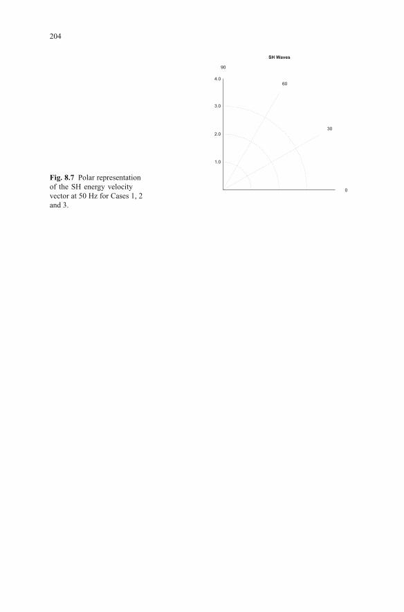
204
Fig. 8.7 Polar representationof the SH energy velocityvector at 50 Hz for Cases 1, 2and 3.
1.0
2.0
3.0
4.0
30
60
90
0
SH Waves
Vex (km/s)Ve
z (k
m/s
)
1. Brine saturated medium with fractures2. Patchy saturated medium without fractures 3. Patchy saturated medium with fractures
1.0 2.0 3.0 4.0
20
40
60
80
100
120
140
30
60
90
0
qP Waves
1000/Q (X)
1000
/Q (Z
)
Patchy saturated mediumwith fractures10% saturationPatchy saturated mediumwith fractures 50% saturation
80 10020 40 60 120 140
20
40
60
80
30
60
90
0
qSV Waves
1000/Q (X)
1000
/Q (Z
)
Patchy saturated mediumwith fractures, 10% saturationPatchy saturated mediumwith fractures, 50% saturation
20 40 8060
(a) (b)
Fig. 8.8 Dissipation factors for qP (a) and qSV (b) waves at 300 Hz for Case 3 and 10% and 50 %CO2 saturation.
to higher attenuation for the patchy saturated case with fractures (Case 3) at a fre-quency of about 40 Hz.
On the other hand, the curves for ‘33’ waves displayed in Figure 8.9(b) showmuch higher attenuation than those for ‘11’ waves for the three cases. The case ofpatchy saturation with fractures (Case 3) is the one exhibiting the highest attenu-ation values for all frequencies. Besides, the case of brine-saturated homogeneousbackground with fractures (Case 1) shows a much higher attenuation than the non-fractured patchy saturated case (Case 2) starting at a frequency of about 26 Hz,
8.7 Numerical experiments

205
while below such frequency the opposite behaviour is observed, though with quitesimilar attenuation.
101 102 103−5
0
5
10
15
20
25
30
35
40
1000
/Q11
Frequency (Hz)
1. Brine saturated medium with fractures2. Patchy saturated medium without fractures 3. Patchy saturated medium with fractures
(a)
101 102 1030
50
100
150
1000
/Q33
Frequency (Hz)
1. Brine saturated medium with fractures2. Patchy saturated medium without fractures 3. Patchy saturated medium with fractures
(b)
Fig. 8.9 Dissipation factor of waves parallel to the fracture plane (‘11’ waves) (a) and of wavesnormal to the fracture plane (‘33’ waves) (b) as function of frequency.
Figure 8.10 shows that for the case of brine-saturated homogeneous backgroundwith fractures (Case 1), ‘11’ velocities are essentially independent of frequency. Inthe case of patchy saturation with fractures (Case 3), velocities are always smallerthan in Case 1, i.e., the presence of CO2 patches induces a velocity decay in thewhole range of frequencies analyzed. On the other hand, velocities for patchy satu-ration with or without fractures show a similar increasing behaviour with frequency.Figure 8.10(b) also shows that ‘33’ waves have the higher frequency dependent be-haviour for the case of a patchy saturated fractured medium (Case 3), with lowervalues than in the other two cases and increasing behaviour after 10 Hz. When thesample is brine saturated with fractures (Case 1), velocities are higher than in case3. On the other hand, the patchy saturated case without fractures exhibits the high-est velocity values with moderate increase with frequency. Thus, for ‘33’ waves
8 The meso-scale. Fractures as thin layers in Biot media and induced anisotropy

206
101 102 1033.6
3.7
3.8
3.9
4.0
3.6
3.7
3.8
3.9
Velo
city
(km
/s)
Frequency (Hz)
1. Brine saturated medium with fractures2. Patchy saturated medium without fractures 3. Patchy saturated medium with fractures
(a)
101 102 1032.5
3.0
3.5
4.0
2.5
3.0
3.5
4.0
2.5
3.0
Velo
city
(km
/s)
Frequency (Hz)
1. Brine saturated medium with fractures2. Patchy saturated medium without fractures 3. Patchy saturated medium with fractures
(b)
Fig. 8.10 Velocity of waves parallel to the fracture plane (‘11’ waves) (a) and waves normal to thefracture plane (‘33’ waves) (b) as function of frequency.
the presence of fractures induces a noticeable reduction of velocities normal to thefracture plane, either for brine or patchy saturation.
The last experiment (Case 4) analyzes the effects of the presence of hetero-geneities in the skeleton or frame of the fractured sample.
As indicated in [Russo and Bouton, 2007, Russo et al., 1997], it is known thatpermeability is log-fractal. Thus, a binary fractal permeability was obtained withthe following logarithmic relation
log κ(x,z) = 〈log κ〉+ f(x,z) (8.44)
with f (x,z) being the fractal representing the spatial fluctuation of the permeabilityfield, chosen to be of fractal dimension D= 2.2, correlation length 2 cm and averagepermeability 0.25 Darcy in the background and 4.44 Darcy in the fractures. In (8.44)〈log κ〉 denotes the average value of the function log κ . Porosity was obtained usingthe Kozeny-Carman relation
8.7 Numerical experiments

207
Thus, the heterogeneous sample was constructed as a fractal perturbation of thesample in Case 1. Figure 8.11fractal sample used in Case 4.
20
40
60
80
100
120
140
160
20 40 60 80 100 120 140 160
Z (cm)
X (cm)
’lambda_global_gnu_2.dat’
3.5
4
4.5
5
5.5
6
6.5
7
(GPa)
Fig. 8.11 Lame coefficient (GPa) for the brine-saturated fractal porosity-permeability sample ofCase 4.
Figure 8.12 compares the qP (a) and qSV (b) dissipation factors of this case at 50Hz with those of Case 1, while Figure 8.12 (c) and (d) compares the correspondingenergy velocities.
As in the patchy saturation case, frame heterogeneities induce a noticeable in-crease in Q anisotropy for qP waves for angles normal to the fracture plane and forqSV waves for angles between 30 and 60 degrees. From Figure 8.12 (a) and (b) weconclude that both qP and qSV wave attenuation are highly increased when frameheterogeneities are present. Also, from Figure 8.12 (c) and (d) we see the expectedenergy velocity reduction in the heterogeneous case, and that velocity anisotropyis less affected by frame heterogeneities than Q anisotropy. Concerning SH waves,they show anisotropy and a moderate reduction in velocity and negligible attenua-tion in the heterogeneous case. The SH energy velocity is similar to that of Figure8.7 in Case 1 and the plot is omitted.
κ(1−φ)2
φ 3 = constant.
shows the Lame coefficient λ of the brine saturatedu
λu
8 The meso-scale. Fractures as thin layers in Biot media and induced anisotropy

208
20
40
60
80
30
60
90
0
qP Waves
1000/Q (X)
1000
/Q (Z
)
1. Brine saturated medium with fractures 4. Fractal porosity−permeability mediumwith fractures
20 40 60 80
20
40
60
80
30
60
90
0
qSV Waves
1000/Q (X)
1000
/Q (Z
)
1. Brine saturated medium with fractures 4. Fractal porosity−permeability mediumwith fractures
20 60 8040
(a) (b)
1.0
2.0
3.0
4.0
30
60
90
0
qP Waves
Vex (km/s)
Vez
(km
/s)
1. Brine saturated medium with fractures 4. Fractal porosity−permeability mediumwith fractures
4.03.02.01.0
1.0
2.0
3.0
4.0
30
60
90
0
qSV Waves
Vex (km/s)
Vez
(km
/s)
1. Brine saturated medium with fractures 4. Fractal porosity−permeability mediumwith fractures
3.0 4.01.0 2.0
(c) (d)
Fig. 8.12 Dissipation factors for qP (a) and qSV (b) waves at 50 Hz for Cases 1 and 4. Figures (c)and (d) correspond to the energy velocities for the respective wave propagation modes.
8.8 Appendix 1. Mesoscopic-flow attenuation theory foranisotropic poroelastic media
White’s mesoscopic attenuation theory of interlayer flow [White et al., 1975] and[Carcione and Picotti, 2006] describes the equivalent viscoelastic medium of a stackof two thin alternating porous layers of thickness d1 and d2, such that the period ofthe stratification is d = d1 +d2. The theory gives the complex and frequency depen-dent stiffness p33. White model has been generalized in [Krzikalla and Muller, 2011]to anisotropic media, i.e., they have obtained the five stiffnesses of the equivalentTIV medium, denoted by pIJ . The stress-strain relations is given by equations (8.3)-
8.8 Appendix 1. Mesoscopic-flow attenuation theory for anisotropic poroelastic media

209
(8.8) and
pIJ(ω) = cIJ +
(cIJ − crIJc33 − cr33
)[p33(ω)− c33],
where crIJ and cIJ are the relaxed and unrelaxed stiffnesses.According to [Gelinsky and Shapiro, 1997] (their eq. (14)), the quasi-static or
relaxed effective constants of a stack of poroelastic layers are
cr66 = B∗1 = 〈μ〉,
cr11 −2cr66 = cr12 = B∗2 = 2
⟨λmμEm
⟩+
⟨λm
Em
⟩2⟨ 1Em
⟩−1
+(B∗
6)2
B∗8
,
cr13 = B∗3 =
⟨λm
Em
⟩⟨1Em
⟩−1
+B∗
6B∗7
B∗8
,
cr33 = B∗4 =
⟨1Em
⟩−1
+B∗
72
B∗8
=
[⟨1Em
⟩−⟨
αEm
⟩2⟨ EG
MEm
⟩−1]−1
,
cr55 = B∗5 = 〈μ−1〉−1,
B∗6 =−B∗
8
(2
⟨αμEm
⟩+
⟨αEm
⟩⟨λm
Em
⟩⟨1Em
⟩−1),
B∗7 =−B∗
8
⟨αEm
⟩⟨1Em
⟩−1
,
B∗8 =
[⟨1M
⟩+
⟨α2
Em
⟩−⟨
αEm
⟩2⟨ 1Em
⟩−1]−1
,
where
λm = Km− 23
μ and Em = Km+43
μ
and we have also reported the notation of that paper for clarity. In the case of nointerlayer flow, i.e., the unrelaxed regime, the stiffnesses are
c66 = cr66,
c11 −2c66 = c12 = 2
⟨(EG−2μ)μ
EG
⟩+
⟨EG−2μ
EG
⟩2⟨ 1EG
⟩−1
,
c13 =
⟨EG−2μ
EG
⟩⟨1EG
⟩−1
,
c33 =
⟨1EG
⟩−1
,
c55 = cr55
[Gelinsky and Shapiro, 1997] ( their eq. (15)), where
EG = Em+α2M,
8 The meso-scale. Fractures as thin layers in Biot media and induced anisotropy

210
and M is given in (1.50).Finally, the P-wave modulus p33 is [White et al., 1975], also see in [Carcione,
p33 =
[1c33
+2(r2 − r1)
2
iω(d1 +d2)(I1 + I2)
]−1
,
where
r =αMEG
and
I =ηκa
coth
(ad2
), a=
√iωηEG
κMEm,
for each single layer.The main assumption by [Krzikalla and Muller, 2011] is that the fluid-flow di-
rection is perpendicular to the fracture layering and that the relaxation behaviour isdescribed by a single relaxation function or stiffness, i.e., p33(ω). Thus the theoryis valid for plane layers and can not be used when 2-D or 3-D heterogeneities arepresent.
8.9 Appendix 2. Wave velocities and quality factors
We consider homogeneous viscoelastic waves [Carcione, 2014]. The complex ve-locities are the key quantity to obtain the wave velocities and quality factor of theequivalent anisotropic medium. They are given by
vqP = (2 ρ)−1/2√
p11l21 + p33l23 + p55 +A,
vqSV = (2 ρ)−1/2√
p11l21 + p33l23 + p55 −A,
vSH = ρ−1/2√
p66l21 + p55l23 ,
A=√[(p11 − p55)l21 +(p55 − p33)l23 ]
2 +4[(p13 + p55)l1l3]2,
where ρ is the average density, l1 = sinθ and l3 = cosθ are the directions cosines,θ is the propagation angle between the wave-number vector and the symmetry axis,and the three velocities correspond to the qP, qSV and SH waves, respectively. Thephase velocity is given by
vp =
[Re
(1v
)]−1
,
while the quality factor is given by
Q=Re(v2)
Im(v2),
2014],
8.9 Appendix 2. Wave velocities and quality factors
211
where v represents either vqP, vqSV or vSH. The energy-velocity vector of the qP andqSV waves is given by
vevp
= (l1 + l3 cotψ)−1e1 +(l1 tanψ + l3)−1e3.
(eq. 6.158) in [Carcione, 2014], where
tanψ =Re(β ∗X +ξ ∗W )
Re(β ∗W +ξ ∗Z),
defines the angle between the energy-velocity vector and the z-axis,
β =√A±B,
ξ =±pv√A∓B,
B= p11l21 − p33l23 + p55 cos2θ
he upper and lower signs correspond to the qP and qS waves, respectively.Moreover,
W = p55(ξ l1/v+β l3/v),X = β p11l1/v+ξ p13l3/v,Z = β p13l1/v+ξ p33l3/v
where “pv” denotes the principal value, which has to chosen according to estab-lished criteria.
On the other hand, the energy velocity of the SH wave is
ve =1
ρvp(l1c66e1 + l3c55e3)
and
tanψ =
(c66
c55
)tanθ
([Carcione, 2014] ( eq. 1.148)), since p55 and p66 are real quantities.In general, the phase velocity is related to the energy velocity by
vp = ve cos(ψ −θ),
where ve = |ve|.
.
T
8 The meso-scale. Fractures as thin layers in Biot media and induced anisotropy
,

Chapter 9
Fractures modeled as boundary conditions inBiot media and induced anisotropy
Abstract The acoustic response of fractures within a Biot medium is modeledusing boundary conditions imposing relations among displacements, stresses andfluid pressure along fractures. Besides, a Biot medium with a dense set of alignedfractures behaves as a transversely isotropic and viscoelastic (TIV) medium whenthe average fracture distance is much smaller than the predominant wavelength ofthe travelling waves. The stiffness coefficients of an equivalent TIV medium to aBiot medium with aligned fractures are determined using a set of boundary-valueproblems formulated in the space-frequency domain at the continuous level, whichare solved using the finite element method.
9.1 Introduction
The acoustic response of fractures within a Biot medium can be modeled using a setof boundary conditions proposed in [Nakagawa and Schoenberg, 2007] to representfluid-solid interaction within a fracture and the effect of its permeability on seismicwave scattering.
These boundary conditions impose: continuity of the total stress components,discontinuities of pressure (or pressures) -proportional to averaged fluid velocitiesacross the fracture- and discontinuities of displacements-proportional to stress com-ponents and averaged fluid pressures along the fracture. They allow to representwave-induced fluid flow, by which the fast waves are converted to slow (diffusive)Biot waves when travelling across fractures (mesoscopic-loss) and heterogeneities[Carcione and Picotti, 2006, Carcione, 2014].
As explained in Chapter 8, dense set of horizontal fractures in a fluid-saturatedporoelastic medium behaves as a TIV medium when the average fracture distance ismuch smaller than the predominant wavelength of the travelling waves. This leadsto frequency and angular variations of velocity and attenuation of seismic waves.
© Springer International Publishing AG 2016
in Geosystems Mathematics and Computing, DOI 10.1007/978-3-319-48457-0_9
213J.E. Santos, P.M. Gauzellino, Numerical Simulation in Applied Geophysics, Lecture Notes

214
Here the quasi-static time-harmonic experiments described in Chapter 8 are ap-plied to a representative sample of a Biot medium with an embedded dense set ofhorizontal fractures modeled as boundary conditions within the sample.
This procedure allows to determine the complex and frequency dependent stiff-nesses of an effective TIV medium equivalent to the original densely fractured Biotmedium. The procedure can be regarded as a numerical up-scaling method to bringthe effect of the meso-scale fractures to the macro-scale.
To discretize each component of the solid displacement vector we employ locallypiecewise bilinear functions that are discontinuous along the fractures. For the fluidphase we use locally the vector part of the Raviart-Thomas-Nedelec space of zeroorder [Raviart and Thomas, 1977], also making them discontinuous along fractures.
9.2 A fractured Biot’s medium
We consider a fractured poroelastic solid saturated by a single phase, compressibleviscous fluid and assume that the whole aggregate is isotropic. Let the super-index(θ),θ = b, f indicate solid matrix and saturant fluid properties associated with thebackground and fractures, respectively.
Let us = (usi ) and u f = (u fi ), i= 1,2,3, denote the averaged displacement vectors
of the solid and fluid phases, respectively. Also let
u f = φ (θ)(u f −us),
be the average relative fluid displacement per unit volume of bulk material, withφ (θ) denoting the effective porosity. Set u= (us,u f ) and note that
ξ =−∇ ·u f ,
represents the change in fluid content.Let ε(us) be the strain tensor of the solid. Also, let τ , and p f denote the stress
tensor of the bulk material and the fluid pressure, respectively.The stress-strain relations in a fractured fluid-saturated poroelastic medium can
be written in the form:
τst(u) = 2μ(θ) εst(us)+δst(
λ (θ)u ∇ ·us− B(θ) ξ
), (9.1)
p f (u) =− B(θ) ∇ ·us+M(θ)ξ , θ = b, f . (9.2)
The coefficient μ(θ) is equal to the shear modulus of the bulk θ -material, consideredto be equal to the shear modulus of the dry θ -material. Also
λ (θ)u = K(θ)
u − 23
μ(θ),
9.2 A fractured Biot’s medium

9 Fractures modeled as boundary conditions in Biot media and induced anisotropy 215
with K(θ)u being the bulk modulus of the saturated θ -material. The coefficients in
(9.1)-(9.2) can be determined as indicated in Chapter 1.Biot’s equations in the diffusive range (ignoring acceleration terms) are (see
Chapter 1, equations (1.79)-(1.80))
∇ · τ(u) = 0, (9.3)
iωη κ−1u f +∇p f (u) = 0, (9.4)
where ω is the angular frequency, η is the fluid viscosity and κ is the frame perme-ability.
9.2.1 The boundary conditions at a fracture inside a Biot medium
Consider a rectangular domain Ω =(0,L1)×(0,L3) with boundary Γ in the (x1,x3)-plane, with x1 and x3 being the horizontal and vertical coordinates, respectively.
Let us assume that the domain Ω contains a set of J( f ) horizontal fracturesΓ ( f ,l), l = 1, · · · ,J( f ) each one of length L1 and aperture h( f ). This set of fracturesdivides Ω in a collection of non-overlapping rectangles R(l), l = 1, · · · ,J f + 1, sothat
Ω = ∪J( f )+1l=1 R(l).
Consider a fracture Γ ( f ,l) and the two rectangles R(l) and R(l+1) having as a com-mon side Γ ( f ,l). Let νl,l+1 and χl,l+1 be the unit outer normal and a unit tangent(oriented counterclockwise) on Γ ( f ,l) from R(l) to R(l+1) , such that νl,l+1,χl,l+1is an orthonormal system on Γ ( f ,l).
Let [us], [u f ] denote the jumps of the solid and fluid displacement vectors atΓ ( f ,l), i.e.
[us] =(u(s,l+1)−u(s,l)
)|Γ ( f ,l) ,
where u(s,l)|Γ ( f ,l) denotes the trace of us as seen from R(l), with similar significancefor u(s,l+1)|Γ ( f ,l) .
The following boundary conditions on Γ ( f ,l), representing the approximate acous-tic response of a fracture as a very thin, compliant and highly permeable layer, arederived in [Nakagawa and Schoenberg, 2007] (their equation (52)):
[us ·νl,l+1] = ηN
((1−α( f )B( f )(1−Π))τ(u)νl,l+1 ·νl,l+1 (9.5)
−α( f ) 12
((−p(l+1)
f )+(−p(l)f ))
Π), Γ ( f ,l),[
us · χl,l+1]= ηT τ(u)νl,l+1 · χl,l+1, Γ ( f ,l), (9.6)
[u f ·νl,l+1
]= α( f )ηN
(−τ(u)νl,l+1 ·νl,l+1 (9.7)

216
+1
B( f )
12
((−p(l+1)
f )+(−p(l)f )))
Π , Γ ( f ,l),
(−p(l+1)f )− (−p(l)f ) =
iω (f)Πκ( f )
12
(u(l+1)f +u(l)f
)·νl,l+1, , Γ ( f ,l), (9.8)
τ(u)νl,l+1 ·νl,l+1 = τ(u)νl+1,l ·νl+1,l , Γ ( f ,l), (9.9)
τ(u)νl,l+1 · χl,l+1 = τ(u)νl+1,l · χl+1,l , Γ ( f ,l). (9.10)
In (9.5)-(9.6) ηN and ηT are the normal and tangential fracture compliances, respec-tively and
α( f ) = 1− K( f )m
K( f )s
.
The fracture dry plane wave modulus H( f )m = K( f )
m +43
μ( f ) and the dry fracture
shear modulus μ( f ) are defined in terms of the fracture aperture h( f ) and the fracturecompliances by the relations
ηN =h( f )
H( f )m
, ηT =h( f )
μ( f ).
Also, the membrane permeability is expressed by
κ( f ) =κ( f )
h( f ).
Besides,
ε =(1+ i)
2
(ω η( f ) α( f ) ηN
2 B( f ) κ( f )
)1/2
, Π(ε) =tanhε
ε,
B( f ) =α( f )M( f )
H( f )u
, H( f )u = K( f )
u +43
μ( f ).
Note that Π = Re(Π)− i Im(Π)≡ ΠR − i ΠI with ΠR > 0,ΠI > 0.In the high-permeability limit (κ →∞), it can be seen that Π → 1 and (9.5)-(9.10)
reduce to equation (53) in [Nakagawa and Schoenberg, 2007]:[us ·νl,l+1
]= ηN
(τ(u)νl,l+1 ·νl,l+1 −α( f )(−p(l+1)
f )), Γ ( f ,l), (9.11)[
us · χl,l+1]= ηT τ(u)νl.l+1 · χl,l+1, Γ ( f ,l), (9.12)
[u f ·νl,l+1
]= α( f )ηN
(−τ(u)νl,l+1 ·νl,l+1 +
1
B( f )(−p(l+1)
f )
), Γ ( f ,l),(9.13)
9.2 A fractured Biot’s medium
η

9 Fractures modeled as boundary conditions in Biot media and induced anisotropy 217
(−p(l+1)f ) = (−p(l)f ), Γ ( f ,l), (9.14)
τ(u)νl,l+1 ·νl,l+1 = τ(u)νl+1,l ·νl+1,l , Γ ( f ,l), (9.15)
τ(u)νl,l+1 · χl,l+1 = τ(u)νl+1,l · χl+1,l . (9.16)
The analysis will be performed for the more general fracture boundary condi-tions (9.5)-(9.10), with the analysis for the boundary conditions (9.11)- (9.16) beinga particular case.
Set
a11 = ηN
(1−α( f )B( f )(1−Π)
), a12 = α( f )ηNΠ , (9.17)
a22 =α( f )ηNΠ
B( f ), Θ = a11a22 −a2
12.
Then from (9.5) and (9.7) we obtain
τ(u)νl,l+1 ·νl,l+1 =a22
Θ[us ·νl,l+1
]+
a12
Θ[u f ·νl,l+1
], Γ ( f ,l), (9.18)
(−p(l+1)f )+(−p(l)f ) = 2
a12
Θ[us ·νl,l+1
]+2
a11
Θ[u f ·νl,l+1
], Γ ( f ,l). (9.19)
Adding (9.8) and (9.19)
(−p(l+1)f ) =
a12
Θ[us ·νl,l+1
]+
a11
Θ[u f ·νl,l+1
](9.20)
+iω ( f )Π
κ( f )
14
(u(l+1)f +u(l)f
)·νl,l+1, Γ ( f ,l).
Using (9.20) in (9.19) we get
(−p(l)f ) =a12
Θ[us ·νl,l+1
]+
a11
Θ[u f ·νl,l+1
](9.21)
− iω ( f )Πκ( f )
14
(u(l+1)f +u(l)f
)·νl,l+1, Γ ( f ,l).
In the analysis that follows we will employ the more convenient form of theboundary conditions given by equations (9.6), (9.9), (9.10), (9.18) (9.20) and (9.21).
9.2.2 The quasi-static experiments to determine the stiffnesses pIJ
The experiments to determine the stiffnesses pIJ defining the equivalent TIV mediumat the macro-scale are those used in Chapter 8 when fractures are modeled as thinhighly permeable and compliant layers. In the next section we describe the varia-
η
η

218
tional formulations that include the fracture boundary conditions (9.6), (9.9), (9.10),(9.18) (9.20) and (9.21).
9.3 A variational formulation
Let us introduce the following closed subspaces of [L2(Ω)]2:
V11(Ω) = v ∈ [L2(Ω)]2 : v|R(l) ∈ [H1(R(l))]2, v ·ν = 0 on Γ\ΓR,
V33(Ω) = v ∈ [L2(Ω)]2 : v|R(l) ∈ [H1(R(l))]2, v ·ν = 0 on Γ\ΓT,
V13(Ω) = v ∈ [L2(Ω)]2 : v|R(l) ∈ [H1(R(l))]2, v ·ν = 0 on ΓL ∪ΓB,
V55(Ω) = v ∈ [L2(Ω)]2 : v|R(l) ∈ [H1(R(l))]2, v= 0 on ΓB,
V66(Ω) = v ∈ [L2(Ω)]2 :: v|R(l) ∈ [H1(R(l))]2, v= 0 on ΓL.
Also, set
H0(div;∪lR(l)) = v ∈ [L2(Ω)]2 : v|R(l) ∈ H(div,R(l)),v ·ν = 0 on Γ,
H10 (div;∪lR
(l))= v ∈ [L2(Ω)]2 : v|R(l)∈ [H1(R(l)]2 : ∇·v ∈ H1(R(l)),v ·ν=0 on Γ.
Next, for (I,J) = (1,1),(3,3),(1,3),(5,5),(6,6) let
ZIJ(Ω) = VIJ(Ω)×H0(div;∪lR(l)).
To obtain the variational formulation associated with p33, multiply equation (9.3)by vs and equation (9.4) by v f with v =
(vs,v f
) ∈ Z33(Ω), integrate over Ω andadd the resulting equations. Next, use integration by parts on each rectangle R(l)
applying the fracture boundary conditions (9.6), (9.9), (9.10), (9.18), (9.20), and(9.21) and the additional boundary conditions (8.10),(8.11) (8.12) and (8.13) to getthe weak form: find u(33) = (u(s,33),u( f ,33)) ∈ Z33(Ω) such that:
Λ(u(33),v)≡ iω(
μ(b) (κ(b))−1u( f ,33),v f)+∑
l
(τst(u(33)),εst(vs)
)R(l)
−(p f (u(33)),∇ ·v f )
)R(l)
+∑l
⟨F([
u(s,33) ·νl,l+1
],[u(s,33) · χl,l+1
],[u(s,33)f ·νl,l+1
]), (9.22)([
vs ·νl,l+1],[vs · χl,l+1
],[v f ·νl,l+1
])⟩Γ ( f ,l)
9.3 A variational formulation

9 Fractures modeled as boundary conditions in Biot media and induced anisotropy 219
+∑l
⟨iω ( f )Π
κ( f )
14
(u( f ,33,l+1) +u( f ,33,l)
)·νl,l+1,
(v( f ,l+1) +v( f ,l)
)·νl,l+1
⟩Γ ( f ,l)
=−〈ΔP,vs ·ν〉Γ T , ∀ v= (vs,v f ) ∈ Z33(Ω).
In (9.22) the 3×3 complex matrix F is given by
F= FR+ iFI =
⎛⎜⎝ f11 0 f12
01
ηT0
f12 0 f22
⎞⎟⎠where ( see (9.17))
It will be assumed that FR is positive definite, that f11.R > 0 and FI is non-negative. This assumptions are valid for any physically meaningful data. Note thatin (9.22), we can write
∑l
(τst(u(33)),εst(vs)
)R(l)
−(p f (u(33)),∇ ·v f (9.23)
=J( f )
∑l=1
(D(b) ε(u(33)), ε(v)
)R(l)
,
where ε(u(33))) =(
ε11(u(s,33)),ε33(u(s,33)),∇ ·u( f ,33),ε13(u(s,33))t
and the matrix
D(b) is defined by
D(b) =
⎛⎜⎜⎜⎝λ (b)u +2μ(b) λ (b)
u B(b) 0
λ (b)u λ (b)
u +2μ(b) B(b) 0B(b) B(b) M(b) 0
0 0 0 4μ(b)
⎞⎟⎟⎟⎠ . (9.24)
Then we can state the variational formulation (9.22) in the equivalent form: findu(33) = (u(33)
s ,u(33)f ) ∈ Z33(Ω) such that:
Λ(u(33),v) ≡ iω(
μ(b)(κ(b))−1u( f ,33),v f)+∑
l
(D(b) ε(u(33)), ε(v)
)R(l)
(9.25)
+∑l
⟨F([
u(s,33) ·νl,l+1
],[u(s,33) ·χl,l+1
],[u( f ,33) ·νl,l+1
]),([
vs ·νl,l+1],[vs · χl,l+1
],[v f ·νl,l+1
])⟩Γ ( f ,l)
+∑l
⟨iω ( f )Π
κ( f )
14
(u( f ,33,l+1) +u( f ,33,l)
)·νl,l+1,
(v( f ,l+1) +v( f ,l)
)·νl,l+1
⟩Γ ( f ,l)
f11 =a22
Θ= f11,R+ i f11,I , f12 =
a12
Θ= f ,R+ i f ,I , f22 =
a11
Θ= f22,R+ i f22,I .12 12
)R(l)
η
η

220
=−〈ΔP,vs ·ν〉Γ T , ∀ v= (vs,v f ) ∈ Z33(Ω).
In a similar fashion we can obtain a weak formulation for the problems associatedwith the other pIJ’s applying the corresponding boundary conditions and the fractureboundary conditions (9.6), (9.9), (9.10), (9.18) (9.20) and (9.21) to get:
• For p11: find u(11) = (u(s,11),u( f ,11)) ∈ Z11(Ω) such that:
Λ(u(11),v) =−〈ΔP,vs ·ν〉Γ R , ∀ v= (vs,v f ) ∈ Z11(Ω). (9.26)
• For p13: find u(13) = (u(s,13),u( f ,13)) ∈ Z13(Ω) such that:
Λ(u(13),v) =−〈ΔP,vs ·ν〉Γ R∪Γ T , ∀ v= (vs,v f ) ∈ Z13(Ω). (9.27)
• For p55: find u(55) = (u(s,55),u( f ,55)) ∈ Z55(Ω) such that:
Λ(u(55),v) =−〈g,vs〉Γ \Γ B , ∀ v= (vs,v f ) ∈ Z55(Ω). (9.28)
• For p66: find u(66) = (u(s,66),u( f ,66)) ∈ Z66(Ω) such that:
Λ(u(66),v) =−〈g2,vs〉Γ \Γ L , ∀ v= (vs,v f ) ∈ Z66(Ω). (9.29)
respectively.Uniqueness of the solution of the variational problems (9.25), (9.26), (9.27),
(9.28) and (9.29) is demonstrated in Appendix 9.7.
9.4 The finite element method
Let T h(Ω) be a non-overlapping partition of Ω into rectangles Ω j of diameterbounded by h such that Ω = ∪J
j=1Ω j. We will assume the Ω j’s are such that theirhorizontal sides either have empty intersection or they coincide with one of thefractures. Let
Ω f = ∪I fj=1Ω j, ΩN f = Ω \Ω f = ∪IN f
j=1Ω j. (9.30)
In (9.30) I f is the number of Ω j’s having one top or bottom side contained in somefracture Γ ( f ,l) for some l in the range 1 ≤ l ≤ J( f ), while IN f is the number of allΩ j’s such that ∂Ω j ∩Γ f ,l = /0 ∀ l.
Let
Nhj = P1,1(Ω j)×P1,1(Ω j), RT N
hj = P1,0(Ω j)×P0,1(Ω j),
9.4 The finite element method
Remark g and g in (9.28) and (9.29) are defined in (8.21) and (8.30),.The functions 2

9 Fractures modeled as boundary conditions in Biot media and induced anisotropy 221
where Ps,t(Ω j) denotes the polynomials of degree up to s in x1 and up to t in x3 onΩ j. Denote by Γjk = ∂Ω j ∩ ∂Ωk the common side of two adjacent rectangles Ω j
and Ωk and ν jk the unit outer normal from Ω j to Ωk. Also, let Γ ( f ,l)jk = Γjk ∩Γ ( f ,l)
and set
Vh,N f
33 (ΩN f ) = vs : vs|Ω j ∈ Nhj ,v
s is continuous across Γjk ∀Ω j ⊂ ΩN f ,Ωk ⊂ ΩN f , vs ·ν = 0 on Γ\ΓT,
Vh, f
33 (Ω f ) = vs : vs|Ω j ∈ Nhj , ∀Ω j ⊂ Ω f , vs ·ν jk is continuous across Γjk
if Ωk ⊂ ΩNf, vs ·ν = 0 on Γ\ΓT,
Vh,N f
11 (ΩN f ) = vs : vs|Ω j ∈ Nhj ,v
s is continuous across Γjk ∀Ω j ⊂ ΩN f ,Ωk ⊂ ΩN f , vs ·ν = 0 on Γ\ΓR,
Vh, f
11 (Ω f ) = vs : vs|Ω j ∈ Nhj , ∀Ω j ⊂ Ω f , vs ·ν jk is continuous across Γjk
if Ωk ⊂ ΩNf,vs ·ν = 0 on Γ\ΓR,
Vh,N f
13 (ΩN f ) = vs : vs|Ω j ∈ Nhj ,v
s is continuous across Γjk ∀Ω j ⊂ ΩN f ,Ωk ⊂ ΩN f , vs ·ν = 0 on ΓL ∪ΓB,
Vh, f
13 (Ω f ) = vs : vs|Ω j ∈ Nhj , ∀Ω j ⊂ Ω f , vs ·ν jk is continuous across Γjk
if Ωk ⊂ ΩNf, vs ·ν = 0 on ΓL ∪ΓB,
Vh,N f
55 (ΩN f ) = vs : vs|Ω j ∈ Nhj ,v
s is continuous across Γjk ∀Ω j ⊂ ΩN f ,Ωk ⊂ ΩN f , vs = 0 on ΓB,
Vh, f
55 (Ω f ) = vs : vs|Ω j ∈ Nhj , ∀Ω j ⊂ Ω f , vs ·ν jk is continuous across Γjk
if Ωk ⊂ ΩNf, vs = 0 on ΓB,
Vh,N f
66 (ΩN f ) = vs : vs|Ω2, j ∈ Nhj ,v
s is continuous across Γjk ∀Ω j ⊂ ΩN f ,Ωk ⊂ ΩN f , vs = 0 on ΓL,
Vh, f
66 (Ω f ) = vs : vs|Ω j ∈ Nhj , ∀Ω j ⊂ Ω f , vs ·ν jk is continuous across Γjk
if Ωk ⊂ ΩNf, vs = 0 on ΓL.
Also set

222
Wh,N f (ΩN f ) = v f : v f |Ω j ∈ RT N
hj ,v
f ·ν jk is continuous across Γjk
∀Ω j ⊂ ΩN f , Ωk ⊂ ΩN f , v f ·ν = 0 on Γ,
Wh, f (Ω f ) = v f : v f |Ω j ∈ RT N
hj , ∀Ω j ⊂ Ω f , v f ·ν jk is continuous across Γjk
if Ωk ⊂ ΩNf, vf ·ν = 0 on Γ.
Next, for (I,J) = (1,1),(3,3),(1,3),(5,5),(6,6) to determine the stiffness pIJ wewill employ the finite element space
ZhIJ(Ω) =
(V
h,NfIJ (ΩNf )∪V
h, fIJ (Ω f )
)×(W
h,Nf (ΩNf )∪Wh, f (Ω f )
). (9.31)
Π hIJ : [H3/2(∪lR
(l))]2 → Vh,NfIJ (ΩNf )∪V
h, fIJ (Ω f
be the bilinear interpolant operators defined locally on each rectangle R(l) and asso-ciated with the spaces V h
IJ .Also, let
Qh : H10 (div;∪R(l))→ W
h,Nf(ΩNf)∪Wh,f(Ωf)
be the projection defined by⟨(Qhψ −ψ) ·ν ,1
⟩B= 0, B= Γjk or B = Γj.
The approximating properties of Π hIJ and Qh are [Ciarlet, 1976, Raviart and Thomas,
‖ϕ −Π hIJϕ‖0 +h
J( f )+1
∑l=1
‖ϕ −Π hIJϕ‖1,R(l) ≤Chs‖ϕ‖s, 1 ≤ s≤ 3/2,
‖ψ −Qhψ‖0 ≤ChJ( f )+1
∑l=1
‖ψ‖1,R(l) ,
‖∇ · (ψ −Qhψ)‖0 ≤ChJ( f )+1
∑l=1
(‖ψ‖1,R(l) +‖∇ ·ψ‖1,R(l)
).
Now, we formulate the FE procedures to determine the stiffnesses pIJ’s as fol-lows:
• p33(ω): find u(h,33) ∈ Z h33(Ω) such that
Λ(u(h,33),v) =−〈ΔP,vs ·ν〉Γ T , ∀ v ∈ Zh
33(Ω). (9.32)
1977, Nedelec, 1980]
9.4 The finite element method
Then, for (I,J) = (1,1),(3,3),(1,3),(5,5),(6,6) let
)

9 Fractures modeled as boundary conditions in Biot media and induced anisotropy 223
• p11(ω): find u(h,11) ∈ Z h11(Ω) such that
Λ(u(h,11),v) =−〈ΔP,vs ·ν〉Γ R , ∀ v ∈ Zh
11(Ω). (9.33)
• p13(ω): find u(h,13) ∈ Z h13(Ω) such that
Λ(u(h,13),v) =−〈ΔP,vs ·ν〉Γ R∪Γ T , ∀ v ∈ Zh
13(Ω). (9.34)
• p55(ω): find u(h,55) ∈ Z h55(Ω) such that
Λ(u(h,55),v) =−〈g,vs〉Γ \Γ B , ∀ v ∈ Zh
55(Ω). (9.35)
• p66(ω): find u(h,66) ∈ Z h66(Ω) such that
Λ(u(h,66),v) =−〈g2,vs〉Γ \Γ L , ∀ v ∈ Zh
66(Ω). (9.36)
Uniqueness for the FE procedures (9.32)-(9.36) can be shown with the same argu-ment used for the continuous case. Existence follows from finite dimensionality.
9.5 A priori error estimates
Here we state the a priori error estimates for the FE procedures (9.32)-(9.36).
and u( f ,IJ) ∈ H10 (div;∪lR(l)). Assume that the coefficients in the constitutive rela-
tions (9.1)-(9.2) satisfy the conditions in (1.58) so that the matrix D(b) in (9.24) ispositive definite. Also assume that FR is positive definite, that f11,R > 0 and that FI
is nonnegative. Then for any ω > 0 and for sufficiently small h > 0 the followingerror estimate holds:
‖u(IJ)−u(h,IJ)‖0+h1/2
[J( f )+1
∑l=1
(‖u(s,IJ)−u(s,h,IJ)‖1,R(l) +‖∇ · (u( f ,IJ)−u( f ,h,IJ)‖0,R(l)
)
+J( f )
∑l=1
∑jk
(‖[(u(s,IJ)−u(s,h,IJ)) ·νl,l+1
]‖
0,Γ ( f ,l)jk
+‖[(u(s,IJ)−u(s,h,IJ)) ·χl,l+1
]‖
0,Γ ( f ,l)jk
+‖[(u( f ,IJ)−u( f ,h,IJ)) ·νl,l+1
]‖
0,Γ ( f ,l)jk
+‖(u( f ,IJ)−u( f ,h,IJ)) ·νl,l+1‖0,Γ ( f ,l)jk
)]
≤C hJ( f )+1
∑l=1
(‖u(s,IJ,l)‖3/2,R(l) +‖u( f ,IJ,l)‖1,R(l) +‖∇ ·u( f ,IJ,l)‖1,R(l)
).
Proof: The proof follows the arguments given in [Santos and Carcione, 2015],modified to take into account the presence of fractures.
Theorem 9.1. Assume that for (I,J)=(1,1),(3,3),(1,3),(5,5),(6,6)u(s,IJ)∈[H3/2(∪lR(l) ]2)

224
9.6 Numerical experiments
In this section we first validate the procedure to determine the stiffnesses pIJ at themacro-scale by comparison with the analytical solution in [Krzikalla and Muller, 2011]¨included in Appendix 8.8. For this purpose the corresponding energy velocitiesand dissipation coefficients are determined as indicated in Appendix 8.9 (see also[Carcione, 2014]).
Next, the complex stiffnesses pIJ(ω), energy velocities and dissipation coeffi-cients are determined for the case of patchy brine-gas saturation for which no ana-lytical solutions are avalaible.
The material properties of background and fractures are given in Table 9.1. Thesaturant fluid is brine, with properties given in Table 9.2.
The numerical samples were discretized with a 100 × 100 uniform mesh.
The first experiment (Figures 9.1 9.2 and 9.3) validate the FE procedure againstthe analytical solution given in Appendix 8.8.
Figures 9.1 and 9.2 show polar plots of the energy velocity vector and dissipation
gation angle, while Figure 9.3 display a polar plot of the energy velocity vector for
9.6 Numerical experiments
Table 9.1 Material properties of background and fractures
Background Solid grains bulk modulus, Ks 36. GPasolid grains density, ρs 2700 kg/m3
Dry bulk modulus Km 9 GPa7 GPa
Porosity φ 0.15permeability κ 0.1 Darcy
Fractures Solid grains bulk modulus, Ks 36. GPasolid grains density, ρs 2700 kg/m3
Dry bulk modulus Km 0.0055 GPashear modulus 0.0033 GPaPorosity φ 0.5permeability κ
Table 9.2 Fluid properties
Brine bulk modulus, Kf 2.25 GPadensity, ρ f
0.0018 Pa · s
Gas bulk modulus, Kf 0.012 GPadensity, ρ f
0.00015 Pa · s
μ
shear modulus μ
10 Darcy
78 kg/m
viscosity, η
viscosity, η
1040 kg/m3
3
factors [(1000/Q)(sinθ , cosθ)] for qP and qSV waves as functions of the propa-

9 Fractures modeled as boundary conditions in Biot media and induced anisotropy 225
SH waves. Frequency is 30 Hz. In the Figures, 0 degrees and 90 degrees correspondto waves arriving parallel and normal to the fracture layering, respectively.
A very good agreement between the numerical and analytical curves is obtainedfor all angles. The qP curves in Figure 9.1 show velocity anisotropy and strong atten-uation for waves arriving close to the normal direction to the fracture layering. Onthe other hand, Figure 9.2 shows that qSV waves have stronger velocity anisotropythan qP waves, have no loss along the directions parallel and normal to the fracturelayering and have maximum attenuation for angles close to 45 degrees. The energyvelocity of qSV waves has the typical cuspidal triangles (or triplications), observedpreviously in fractured media [Carcione, 1996]. Figure 9.3 shows that SH waveshave velocity anisotropy; they are lossless.
1
2
3
4
30
60
90
0
Vex (km/s)
Vez
(km
/s)
TheoryFE
2 3 41
100
200
300
30
60
90
0
1000/Q(X)
1000
/Q(Z
)
TheoryFE
100 200 300
(a) (b)
The second experiment considers the same sample but for full brine saturation,full gas saturation and 10 % and 50 % patchy brine-gas saturation. Brine and gashave properties given in Table 9.2. Frequency is 30 Hz and a 100× 100 mesh wasemployed.
Patchy gas-brine distributions were generated using e Von Karman spectrum den-sity formula (7.21) and the procedure explained in Subsection 7.7.1. In this examplethe parameter values in (7.21) were chosen to be Ne = 2, D = 2.2 and correlationlength CL equal to one percent of the domain size.
Following this procedure two different patchy gas-brine distributions of overall10 % and 50 % gas saturations were generated.
Figures 9.4 and 9.5 display polar plots of energy velocity vectors and qualityfactor of qP and qSV waves, respectively, as a function of the propagation anglefor 0 %, 10 %, 50 % and 100 % global gas saturations. Frequency is 30 Hz. Figure
Fig. 9.1 Polar representation of the energy velocity (a) and dissipation factor[(1000/Q)(sinθ, cosθ )] (b) of qP waves as function of the propagation angle. Frequencyis 30 Hz. The symbols correspond to the analytical values, while solid lines indicate the FEexperiments.

226
0.5
1
1.5
2
2.5
30
60
90
0
Vex (km/s)
Vez
(km
/s)
TheoryFE
1 1.5 2 2.50.5
100
200
300
30
60
90
0
1000/Q(X)
1000
/Q(Z
)
TheoryFE
100 200 300
(a) (b)
0.5
1
1.5
2
30
60
90
0
Vex (km/s)
Vez
(km
/s)
TheoryFE
0.5 1.5 21
Fig. 9.3 Polar representation of the energy velocity of SH waves as function of the propagationangle. Frequency is 30 Hz. The symbols correspond to the analytical values, while solid linesindicate the FE experiments.
9.4 (a) indicates that velocity of qP waves decreases as gas saturation increases,while Figure 9.4 (b) shows that qP anisotropy is enhanced by patchy saturation, ismaximum for qP waves arriving normally to the fracture layering and decreases asgas saturation increases. Maximum attenuation occurs at 10 % gas saturation for allangles.
For qSV waves, Figure 9.5 (a) shows that velocity decreases as gas saturationincreases, with different anisotropic behaviour depending on the value of gas satu-
9.6 Numerical experiments
Fig. 9.2 Polar representation of the energy velocity (a) and dissipation factor[(1000/Q)(sinθ ,cosθ)] (b) of qSV waves as function of the propagation angle. Frequency is 30Hz. The symbols correspond to the the analytical values, while solid lines indicate FE experiments.

9 Fractures modeled as boundary conditions in Biot media and induced anisotropy 227
1
2
3
4
30
60
90
0
Vex (km/s)
Vez
(km
/s)
0% Gas10% Gas50% Gas100% Gas
1 2 3 4
200
400
600
30
60
90
0
1000/Q(X)
1000
/Q(Z
)
0% Gas10% Gas50% Gas100% Gas
400 600200
(a) (b)
Fig. 9.4 Polar representation of the energy velocity (a) and dissipation factor[(1000/Q)(sinθ ,cosθ)] (b) of qP waves as function of the propagation angle for full brine,full gas, 10 % and 50 % patchy gas-brine saturation. Frequency is 30 Hz.
0.5
1
1.5
2
2.5
30
60
90
0
Vex (km/s)
Vez
(km
/s)
0% Gas10% Gas50% Gas100% Gas
1 20.5 1.5 2.5
100
200
300
400
500
30
60
90
0
1000/Q(X)
1000
/Q(Z
)
0% Gas10% Gas50% Gas100% Gas
100 200 300 400 500
(a) (b)
Fig. 9.5 Polar representation of the energy velocity (a) and dissipation factor[(1000/Q)(sinθ ,cosθ)] (b) of qSV waves as function of the propagation angle for full brine, fullgas, 10 % and 50 % patchy gas-brine saturation. Frequency is 30 Hz.
ration. Concerning the dissipation factor for qSV waves, Figure 9.5 (b) shows maxi-mum attenuation at 10 % gas saturation, and decreasing anisotropy as gas saturationincreases. Besides, qSV anisotropy shows different behaviour for different valuesof gas saturation. The patchy nature of the saturation breaks the symmetry of thecurves (see the cuspidal triangles), with the attenuation of the qSV wave havinghigher values at different angles.

228
10
20
30
40
50
60
70
80
90
100
10 20 30 40 50 60 70 80 90 100
0 10 20 30 40 50 60 70 80 90 100
nz
nx
’Salida_presion’
0
0.2
0.4
0.6
0.8
1
1.2
1.4
1.6
1.8
Pf [Pa]
Fig. 9.6 Fluid pressure for normal compression to the fracture plane at 10 % patchy gas-brinesaturation. Frequency is 30 Hz.
On the other hand, the SH wave is lossless and energy velocity of SH waves isunaffected by different values of gas saturation, the corresponding curves coincidewith that in Figure 9.3 and are ommited.
Figure 9.6 shows the fluid pressure distribution (in Pa) for compressions normalto the fracture layering (p33 experiment) for 10 % patchy gas saturation, where thehigher pressure values occur at the fracture locations and the darker regions valuesidentify the gas patches. This figure illustrates the mesoscopic attenuation mecha-nism affecting compressional and shear waves at the macro-scale and characterizedin the previous patchy-related experiments.
9.7 Appendix 1. Uniqueness of the solution of the variationalproblems
9.7 Appendix 1. Uniqueness of the solution of the variational problems
Remark l, u(s,33) ∈[H3/2(R(l))]2,u(s,33)
f ∈[H1(R(l))]2, so that u(s,33) ·νl,l+1∈H1(Γ ( f ,l))⊂L2(Γ ( f ,l)),u( f ,33)·νl,l+1 ∈ H1/2(Γ ( f ,l)) ⊂ L2(Γ ( f ,l)). Thus, since vs ∈ H1(R(l)),v f ∈ H0(div;∪lR(l)),vs ·νl,l+1 ∈H(1/2)(Γ ( f ,l))⊂ L2(Γ ( f ,l)),v f ·νl,l+1 ∈H−(1/2)(Γ ( f ,l)). Then all bound-ary terms in (9.22) or (9.25) make sense either in L2(Γ ( f ,l))× L2(Γ ( f ,l)) or in
. In the analysis that follows it will be assumed that for all

9 Fractures modeled as boundary conditions in Biot media and induced anisotropy 229
H(1/2)(Γ ( f ,l))×H−(1/2)(Γ ( f ,l)). Identical assumptions will be made on u(IJ)s and
u(IJ)f for (I,J) = (1,1),(1,3),(5,5),(6,6).Let us analyze the uniqueness of the solution of (9.25). Set ΔP = 0 and choose
v= u(33) in (9.25) to obtain the equation
(iω(
μ(b)(κ(b))−1u( f ,33),u( f ,33))+∑
l
(D(b) ε(u(33)), ε(u(33))
)R(l)
+∑l
⟨(FR+ iFI)
([u(s,33) ·νl,l+1
],[u(s,33) · χl,l+1
],[u( f ,33) ·νl,l+1
]),([
u(s,33) ·νl,l+1
],[u(s,33) · χl,l+1
],[u( f ,33) ·νl,l+1
])⟩Γ ( f ,l)
(9.37)
+∑l
⟨(iω ( f )(ΠR− iΠI)
κ( f )
14
(u( f ,33,l+1)+u( f ,33,l)
)·νl,l+1,
(u( f ,33,l+1)+u( f ,33,l)
)·νl,l+1
⟩= 0.
Take imaginary part in (9.37) and use that FI is nonnegative and ΠR > 0 to seethat
‖u( f ,33)‖0 = 0. (9.38)
Using (9.38), (9.37) reduces to
∑l
(D(b) ε(u(33)), ε(u(33))
)R(l)
+
⟨1
ηT
[u(s,33) · χl,l+1
],[u(s,33) · χl,l+1
]⟩Γ ( f ,l)
(9.39)[u(s,33) ·νl,l+1
],[u(s,33) ·νl,l+1
])⟩
Γ ( f ,l)= 0,
where
D(b) =
⎛⎜⎝λ (b)u +2μ(b) λ (b)
u 0
λ (b)u λ (b)
u +2μ(b) 00 0 4μ(b)
⎞⎟⎠ , ε(u(33)s ) =
⎛⎝ ε11(u(s,33))
ε33(u(s,33))
ε13(u(s,33))
⎞⎠ .
Next, take real part in (9.39) and use that f11,R > 0,ηT > 0 and that the matrix D(b)
is positive definite (since D(b) is positive definite) to conclude that
‖ε11(u(s,33))‖0,R(l) = ‖ε33(u(s,33))‖0,R(l) = ‖ε13(u(s,33))‖0,R(l) = 0, ∀ l. (9.40)
Now use (9.40), the uniqueness argument given in Appendix (7.10) and the Sobolevembedding [Adams, 1975]
H3/2(R(l))→C0B(R
(l))
to see that for some constants A(l),B(l),C(l),
Γ ( f ,l)
+∑l
⟨( f11,R+ i f11,I)
η

230
u(s,33)1 (x1,x3) =C(l)x3 +B(l),
u(s,33)3 (x1,x3) =−C(l)x1 +B(l), ∀(x1,x3) ∈ R
(l), ∀ l.
Next using the boundary condition (8.12) we see that A(l) = B(l) =C(l) = 0, so that
u(s,33) = 0, (x1,x3) ∈ R(l) ∀ l. (9.41)
Combining (9.38) and (9.41) we conclude that uniqueness holds for the solutionof (9.25). Uniqueness for the solution of (9.26) and (9.27) follows with the sameargument.
Let us analyze uniqueness for the solution of (9.28). Repeating the argumentgiven to show uniqueness for u(33) we obtain
‖u( f ,55)‖0 = 0, (9.42)
‖ε11(u(s,55))‖0,R(l) = ‖ε33(u(s,55))‖0,R(l) = ‖ε13(u(s,55))‖0,R(l) = 0, ∀ l.
Next, consider the rectangle R(1), which bottom boundary is Γ B. Let u(s,55,l) ≡(u(s,55))|R(l) . Thanks to the boundary condition (8.19),
‖|v‖|R(1) =(
∑j,k
∫R(1)
|ε jk(v)|2dx1dx3
)1/2
defines a norm in R(1) equivalent to the H1-norm [Ciarlet, 1976]. Thus from (9.42)we see that
‖u(s,55)‖1,R(1) = 0,
and since u(s,55) ∈ [H3/2(R(1))]2 → [C0B(R
(1))]2, we conclude that
u(s,55)1 = 0, (x1,x3) ∈ R
(1). (9.43)
In particular,
u(s,55)1 = u(s,55)
3 = 0, on Γ1,2. (9.44)
From (9.42) and (9.43) we see that (9.28) for the choice v= u(55) reduces to
J( f )
∑l=2
⟨( f11,R+ i f11,I)
[u(s,55) ·νl,l+1
],[u(s,55) ·νl,l+1
]⟩Γ ( f ,l)
+
⟨1
ηT
[u(s,55) · χl,l+1
],[u(s,55) · χl,l+1
]⟩Γ ( f ,l)
= 0. (9.45)
Take real part in (9.45), use that f11,R > 0,ηT > 0 to get
9.7 Appendix 1. Uniqueness of the solution of the variational problems

9 Fractures modeled as boundary conditions in Biot media and induced anisotropy 231[u(s,55) ·νl,l+1
]=[u(s,55) · χl,l+1
]= 0, L2(Γ 1,2). (9.46)
Since u(s,55) ∈ [H3/2(R(2))]2 → [C0B(R
(2))]2 using (9.44) and (9.46) we conclude that
u(s,55,2)1 = u(s,55,2)
3 = 0, on Γ1,2. (9.47)
Now using (9.47) we can apply in R(2) the argument given for R(1) to conclude that
u(55,2)s = 0, (x1,x3) ∈ R
(2).
In this way in l-steps we conclude that
u(55,l)s = 0, ∈ R
(l), l = 1, · · · ,J f +1,
so that uniqueness holds for the solution of (9.28). Uniqueness for the solution of(9.29) follows with identical argument.

Chapter 10
The macro-scale. Seismic monitoring of CO2sequestration
Abstract Storage of carbon dioxide (CO2) in deep saline aquifers and aging oilreservoirs is a valid alternative approach for reducing the amount of greenhousegases in the atmosphere. This procedure can be modeled by the combined useof multi-phase fluid flow and wave propagation. The flow simulator is used tomodel the CO2 injection, and seismic monitoring is applied to determine the spatio-temporal distribution of CO2 after several years of injection. The simultaneous flowof brine and CO2 is modeled with the Black-Oil formulation for two-phase flow inporous media, while wave propagation is formulated using an isotropic viscoelasticmodel. The CO2 saturation and pressure data computed with the flow simulator isused in a petrophysical model to determine the complex bulk and shear moduli ofthe formation. Wave propagation is performed using a finite element domain de-composition procedure. The simulation is used to model CO2 injection and flowand compute time-lapse seismograms corresponding to the Utsira aquifer at Sleip-ner field with the objective of identifying the spatio-temporal distribution of CO2
after injection.
10.1 Introduction
Capture and storage of carbon dioxide in deep saline aquifers and aging oil reser-voirs is a valid alternative approach for reducing the amount of greenhouse gasesin the atmosphere [Arts et al., 2008]. Saline aquifers are suitable as storage sitesdue to their large volume and their common occurrence in nature. The first indus-trial scale CO2 injection project is the Sleipner gas field in the North Sea, whereCO2 separated from natural gas, is being injected in the Utsira formation, a highlypermeable porous sandstone, 800 m below the sea bottom. Within the formation,there are several mudstone layers which act as barriers to the vertical flow ofthe CO2. Injection started in 1996 at a rate of about one million tonnes per year[Arts et al., 2008, Chadwick et al., 2005].
© Springer International Publishing AG 2016
in Geosystems Mathematics and Computing, DOI 10.1007/978-3-319-48457-0_10
233J.E. Santos, P.M. Gauzellino, Numerical Simulation in Applied Geophysics, Lecture Notes

234
Numerical modeling of CO2 injection and seismic monitoring are important toolsto understand the long term behaviour after injection and to test the effectiveness ofCO2 sequestration. In [Carcione and Picotti, 2006] and [Carcione et al., 2012] seis-mic modeling is applied to monitor the spatio-temporal distribution of CO2 assum-ing known CO2 saturation maps after injection. Instead, this Chapter describes amethodology to model the CO2 flow and monitor the storage combining numeri-cal simulations of CO2-brine flow and seismic wave propagation. A petrophysicalmodel of the Utsira formation is built based on fractal porosity and clay content,taking into account the variation of properties with pore pressure and saturation[Carcione et al., 2003]. This model includes embedded mudstone layers of very lowpermeability where CO2 is accumulated, although upward migration also occurs.The simultaneous flow of brine and CO2 is modeled with the Black-Oil formulationfor two-phase flow in porous media [Aziz and Settari, 1985], which uses the PVTdata as a simplified thermodynamic model [Hassanzadeh et al., 2008]. The pressuremap before the injection is assumed to be hydrostatic for which a reference porositymap is defined. The permeability is assumed to be anisotropic and is obtained fromfirst principles as a function of porosity and grain sizes [Carcione et al., 2003].
The wave propagation simulator is based on an isotropic viscoelastic model thatconsiders dispersion and attenuation effects. The complex P-wave and S-wave mod-uli are determined as follows: in the brine saturated mudstone layers and the baseand top of the Utsira sand we use a Zener model to represent the viscoelastic be-haviour of the material [Carcione, 2014]; outside the mudstone layers, we use thetime-harmonic compressibility tests described in Chapter 7 to model P-wave atten-uation. The complex shear modulus is determined using another mechanism relatedto the P-wave mechanism [Carcione et al., 2012].
The CO2 saturation and pressure data computed with the flow simulator wereused in the petrophysical (poro-viscoelastic) model to determine the complex bulkand shear moduli of the formation in order to compute the synthetic seismograms.
The methodology was used to model CO2 injection and flow and compute time-lapse seismograms corresponding to the Utsira aquifer at Sleipner field. It waspossible to identify the spatio-temporal distribution of CO2 after its injection overlong periods of time. Attenuation and dispersion effects are clearly observed in therecorded traces. The synthetic seismograms show the progressive increase in CO2
accumulations below the mudstone layers and the pushdown effect observed in fielddata [Chadwick et al., 2009]. Better results are obtained by updating the petrophys-ical properties (mainly porosity, permeability and dry-rock moduli). Since the ef-fectiveness of the time-lapse seismic method depends on the survey plan and theproperties of the storage site [Chadwick et al., 2010], these simulations may be usedto optimize the type of sources and the number and location of receivers to performthe seismic surveys.
10.1 Introduction

235
10.2 The Black-Oil formulation of two-phase flow in porousmedia
The simultaneous flow of brine and CO2 in porous media is described by thewell-known Black-Oil formulation applied to two-phase, two component fluid flow[Aziz and Settari, 1985]. We identify the CO2 saturated aqueous phase (CO2 andbrine components, subindex b) with the oil phase and the CO2 phase (subindex g)with the gas phase. In this way, the CO2 component may dissolve in the aqueousphase but the brine component is not allowed to vaporize into the CO2 phase. Thedifferential equations are obtained by combining the mass conservation equationswith Darcy’s empirical law.
The mass conservation equations are:
For the CO2 component,
−∇ · (ρg vg+Cg,b ρb vb)+qg =∂[φ(ρgSg+Cg,b ρb Sb
)]∂ t
, (10.1)
for the brine component,
−∇ · (Cb,b ρb vb)+qb =∂[φ(Cb,b ρb Sb)
]∂ t
, (10.2)
where ρ is density at reservoir conditions, v is Darcy velocity, S is saturation, q massrate of injection per unit volume and φ is porosity. Cg,b, Cb,b are the mass fractionsof CO2 and brine in the brine phase, respectively. In the Black-Oil formulation thesefractions are computed using a simplified thermodynamic model as
Cg,b =Rs ρSC
g
Bb ρb, Cb,b =
ρSCb
Bbρb, ρg =
ρSCg
Bg, (10.3)
where
• Rs: CO2 solubility in brine,• Bg: CO2 formation volume factor,• Bb: brine formation volume factor
are the PVT data.Also ρSC
g and ρSCb are the CO2 and brine densities at standard conditions.
To estimate the Black-Oil PVT data we apply an algorithm developed in [Hassanzadehwhich is summarized in Subsection 10.5.2.
The empirical Darcy’s law gives the momentum balance for the fluids,
vg =−κKrg
ηg(∇pg−ρgg∇D), (10.4)
et al., 2008],
10 The macro-scale. Seismic monitoring of CO2 sequestration

236
vb =−κKrb
ηb(∇pb−ρbg∇D), (10.5)
where D indicates depth, generally identified with the coordinate x3, and g is thegravity constant. Also, pg, pb are the fluid pressures and κ is the absolute permeabil-ity tensor, assumed to be diagonal κ = diag(κx,κy,κz). For β = g,b, the functionsKrβ and ηβ are the relative permeability and viscosity of the β -phase, respectively.
Replacing equations (10.3)-(10.5) into equations (10.1)-(10.2) and dividing byρSCg and ρSC
b , the following nonlinear system of partial differential equations is ob-tained,
∇ · (κ( Krg
Bgηg(∇pg−ρgg∇D)+
RsKrb
Bbηb(∇pb−ρbg∇D)))+
qgρSCg
(10.6)
=
∂[φ(SgBg
+RsSbBb
)]∂ t
,
∇ · (κ Krb
Bbηb(∇pb−ρbg∇D))+
qbρSCb
=
∂[φSbBb
]∂ t
. (10.7)
Two algebraic equations relating the saturations and pressures, complete the sys-tem:
Sb+Sg = 1, pg− pb = PC(Sb),
where PC is the capillary pressure.The unknowns for the Black-Oil model are the fluid pressures pg, pb and the
saturations Sg, Sb for the CO2 and brine phases, respectively. This flow model doesnot take into account chemical reactions.
The numerical solution is obtained with public-domain software BOAST [Fanchi,
to accurately represent reservoir geometry. The basic idea of IMPES is to obtain asingle pressure equation by a combination of the flow equations, therefore equation(10.6) multiplied by Bg and equation (10.7) multiplied by (Bb−RsBg) are added.After some algebraic manipulations (the details can be found in Appendix 10.8) andreplacing pg by pb+PC(Sb) in the left side of the combined equation, the followingpressure equation in pb is obtained,
1997] which solves the differential equations using the IMPES algorithm (IMplicitPressure Explicit Saturation), based on a finite difference technique [Aziz and Settari,1985]. Finite differences is the standard in commercial reservoir simulators, and theimproved versions use both structured and unstructured grids with local refinements
10.2 The Black-Oil formulation of two-phase flow in porous media

237
Bg
[∇ · (κ( Krg
Bgηg(∇pb−ρgg∇D)+
RsKrb
Bbηb(∇pb−ρbg∇D)+
Krg
Bgηg∇PC))
]+(Bb−RsBg)
[∇ · (κ Krb
Bbηb(∇pb−ρbg∇D))
](10.8)
+Bgqg
ρSCg
+(Bb−RsBg)qb
ρSCb
= φct∂ pb∂ t
,
where ct is the total compressibility (see the definitions of compressibilities in Ap-pendix 10.8).
In the BOAST simulator, the nonlinear differential equations (10.7) and (10.8)are discretized applying a backward finite difference scheme in a block centeredgrid. The discretized equations are linearized evaluating the pressure and satu-ration dependent coefficients (PVT parameters, viscosities, relative permeabilitiesand capillary pressure) using the pressure and saturation values at the previoustime step. First, the pressure equation (10.8) is solved implicitly. The Block Suc-cessive Over Relaxation method (BSOR) is applied to compute the solution ofthe resulting linear system. Once the pressures for the new time are obtained, wecompute the saturations explicitly from the discretization of equation (10.7). Con-sequently, the time step has to be selected according to the stability restrictions[Savioli and Bidner, 2005].
10.3 A viscoelastic model for wave propagation
One of the main phenomena occurring in rocks, in particular partially saturatedwith gas, is the mesoscopic-loss effect. To model this effect a viscoelastic isotropicmedium long-wave equivalent to an heterogeneous fluid-saturated poroelastic mediumis used. Let us formulate the differential model for wave propagation.
Let ρs and ρ f be the grain and fluid densities, respectively. The equation of mo-tion in a 2-D isotropic viscoelastic domain Ω in the (x1,x3) plane with boundary∂Ω = Γ can be stated in the space-frequency domain (x1,x3,ω) as
−ω2ρu−∇ ·σ(u) = f(x1,x3,ω), (x1,x3) ∈ Ω , (10.9)
−(σ(u)ν ·ν ,σ(u)ν · χ) = iωB(ω)(u ·ν ,u · χ) , (x1,x3) ∈ Γ , (10.10)
where u= (u1,u3) is the displacement vector and
ρ = (1−φ)ρs+φρ f
is the bulk density and B(ω) is defined as a generalization of the absorbing bound-ary condition for elastic solids derived in (5.37) to frequency dependent Lame coef-ficients λ (ω) and μ(ω) as
10 The macro-scale. Seismic monitoring of CO2 sequestration

238
B(ω) =
⎛⎜⎜⎝λ (ω)+2μ(ω)
ρ0
0μ(ω)
ρ
⎞⎟⎟⎠=
(vp(ω) 0
0 vs(ω)
)
where vp(ω),vs(ω) the phase velocities of the compressional and shear waves at thefrequency ω as defined in (7.10)-(7.12).
The stress tensor σ(u) is defined in the space-frequency domain by
where denotes the strain tensor and δ jk is the Kronecker delta.The Lame coefficients λu(ω) and μ(ω) are complex and frequency dependent
and are determined as follows.Let Km and μm denote the bulk and shear moduli of the dry matrix. In the brine
saturated mudstone layers and in the base and top of the Utsira sand we use a Zenermodel to make the Gassmann bulk modulus Ku = Km+α2M and the shear modulusμm complex and frequency dependent. For this purpose, we define quality factorsQ(1)Ku
associated with Ku and Q(2)s associated with μm as
Q(2)s =
μm
KmQ(1)Ku
(10.11)
and proceed as in Appendix 1.9; (see (1.50) and (1.51) for the definition of Ku,αand M).
Within the Utsira sandstone and outside the mudstone layers P-wave attenuationdue to wave induced fluid flow at mesoscopic scale is modeled by computing thecomplex plane wave modulus
Eu(ω) = (λu+2 μ)(ω) (10.12)
using the time-harmonic experiments defined in Section 7.2.Shear wave attenuation and dispersion is also taken into account by making the
shear modulus μ(ω) in (10.12) complex and frequency dependent using the follow-ing argument.
We assume that μ(ω) is represented by a Zener element having a minimum qual-
ity factor given by (10.11) where Q(1)Ku is the minimum (in frequency) quality factor
associated with the complex bulk modulus Ku(ω) computed as
Q(1)Ku = minω
Re(Ku(ω)
Im(Ku(ω))
where
Ku(ω) = Eu(ω)− 43
μm.
10.3 A viscoelastic model for wave propagation
σjk( ) = λu(ω)∇ · u δjk + 2µ(ω)ejk(u), Ω,
ejk(u)
u

239
The Zener model and the time-harmonic experiments to determine the P-wavemodulus require the knowledge of the bulk modulus Ks and density ρs of the solidgrains, the bulk and shear modulimeabilities κx,κz of the solid matrix. They also need the fluid bulk modulus andviscosity. The determination of these parameters is explained in 10.5.1.
10.4 Continuous and discrete variational formulations forviscoelastic wave propagation
10.4.1 Continuous variational formulation
We proceed to formulate the variational form for viscoelastic wave propagation:Find u ∈ [H1(Ω)]2 such that
Λ(u,v) =−(ρω2 ,v)+∑pq(σpq(u), pq(v))
+iω 〈Bu,v〉= (f,v), v ∈ [H1(Ω)]2. (10.13)
In what follows it is convenient to express the term ∑pq(σpq(u), in a differ-ent form by using a matrix D and the column vector (u) defined as follows:
D=
⎛⎝λ +2μ λ 0λ λ +2μ 00 0 4μ
⎞⎠ and =
Denoting by DR and DI the real and imaginary parts of D, respectively, we observethat
(10.14)
Furthermore, we assume that DR is positive definite; in the elastic case DR is asso-ciated with the strain energy density, which is a strictly positive quadratic form ofthe deformation tensor. In the meanwhile, the fact that DI is positive definite is aconsequence of the restrictions imposed on the system of viscoelasticity by the Firstand Second Laws of Thermodynamics [Fabrizio and Morro, 1992].
Denote by BR and BI the real and imaginary parts of B. Assume that
Km and μm as well as the porosity φ and per-
e
pq(v))e
e(u)
(σ(u), e(v)) = (DRe(u), e(v)) + i (DI e(u), e(v)) .
is positive definite and BI
andBR (10.14), the well–posedness of Problem (10.9)-(10.10) follows with an
BR
argument similar to that given in [Douglas Jr. et al., 1994].
.
e11(u)e33(u)e13(u)
e
is nonnegative . By the positive definitenes s of –
10 The macro-scale. Seismic monitoring of CO2 sequestration
u
240
10.4.2 Discrete variational formulation. The global finite elementmethod
Let (T h)h>0 be non-overlapping partition of Ω into rectangles Ω j, j = 1, · · · ,J,of diameter ≤ h such that Ω =∪J
j=1Ω j and Ω j∩Ωk = /0, j = k. Set Γjk = ∂Ω j∩∂Ωk
and Γj = ∂Ω j ∩Γ and let ξ jk and ξ j the mid points of Γjk and Γj, respectively. Todefine a global finite element method we employ the non-conforming finite elementspace MC
h defined over the partition . The space MCh based on rectangular
elements is defined in Chapter 6 in (6.68).The global non-conforming Galerkin procedure is defined as follows: find uh ∈
[MCh]2 such that
Λ(uh,v) =−(ρω2uh,v)+∑pq(σpq(uh),
+iω⟨⟨
Buh,v⟩⟩
= (f,v), v ∈ [MCh]2, (10.15)
where 〈〈·, ·〉〉 denotes the approximation of 〈·, ·〉 on the boundary faces by the mid-point quadrature rule
〈〈u,v〉〉Γ = ∑j(uv)(ξ j)|Γj|
where |Γj| is the measure of Γj.Instead of solving the global problem, we will use the parallelizable domain
decomposition iterative hybridized procedure defined in [Ha et al., 2002]. This ap-proach becomes a necessity when dealing with large 2-D (or 3-D) problems. Thefollowing theorem states the a priori error estimate for the procedure (10.15). Theproof is given in [Ha et al., 2002].
Theorem 10.1. Let u and uh be solutions of (10.13) and (10.15), respectively. Then,for sufficiently small h> 0, we have
‖u−uh‖0 ≤ C(ω)h2‖u‖2, (10.16)
∑j‖u−uh‖1,Ω j ≤ C(ω)h‖u‖2. (10.17)
In (10.16) and (10.17) C(ω) is a computable constant depending only on ω and thedomain Ω .
10.4.3 Domain decomposition
Consider the decomposition of problem (10.9)-(10.10)- over Ω j as follows: for j =1, . . . ,J, find u j(x,ω) satisfying
−ρω2u j(x1,x3,ω)−∇ ·σ(u j(x1,x3,ω)) = f(x1,x3,ω), (x1,x3) ∈ Ω j, (10.18)
T h
epq( )v )
10.4 Continuous and discrete variational formulations for viscoelastic wave propagation

241
iωBu j(x1,x3,ω)+σ(u j(x1,x3,ω))ν j = 0, (x1,x3) ∈ Γj, (10.19)
with the consistency conditions
u j(x1,x3,ω) = uk(x1,x3,ω), (x1,x3) ∈ Γjk ∀k, (10.20)
σ(u j(x1,x3,ω))ν jk+σ(uk(x1,x3,ω))νk j = 0, (x1,x3) ∈ Γjk. (10.21)
Instead of (10.20)–(10.21), we will impose the equivalent Robin transmissionboundary conditions
σ(u j(x1,x3,ω))ν jk+β jku j(x1,x3,ω)
=−σ(uk(x1,x3,ω))νk j+β jkuk(x1,x3,ω), (x1,x3) ∈ Γjk ⊂ ∂Ω j, (10.22)
σ(uk(x1,x3,ω) νk j+β jkuk(x1,x3,ω)
=−σ(u j(x1,x3,ω))ν jk+β jku j(x1,x3,ω), (x1,x3) ∈ Γk j ⊂ ∂Ωk, (10.23)
with β jk being a complex matrix function defined on the interior boundaries Γjk
such that its real and imaginary parts are positive semi-definite and positive definitematrices, respectively.
A weak form of (10.18)–(10.19) and (10.22)–(10.23) is stated as follows: for allj, find u j ∈ [H1(Ω j)]
2 such that
−ω2(ρu j,v) j+(σ(u j), ) j+ iω⟨Bu j,v
⟩Γj
+∑k
〈σ(uk)ν jk+β jk(u j−uk),v〉Γjk = (f,v) j, v ∈ [H1(Ω j)]2. (10.24)
In (10.24) we used the notation
( f ,g) j =∫
Ω j
f gd(∂Ω j).
Since the object of the domain decomposition procedure is to localize the calcu-lations, we define the iterative procedure at the differential level in the followingfashion: given u0
j ∈ [H1(Ω j)]2 for all j, find unj ∈ [H1(Ω j)]
2 such that
−ω2(ρunj ,v) j+(σ(unj),
)j+ iω
⟨Bunj ,v
⟩Γj
+∑k
〈[σ(un−1k )ν jk+β jk(u
nj −un−1
k )],v〉Γjk = (f,v) j, v ∈ [H1(Ω j)]2.(10.25)
Next we define a hybridized non-conforming domain decomposition proceduremotivated by (10.25). For that purpose, we introduce a set L of Lagrange multi-pliers ηh
jk associated with the stress values −σ(u j)ν jk at the midpoints ξ jk of theinterior faces Γjk. Set
= ηh : ηh|Γjk = ηhjk ∈ [P0(Γjk)]
2 ≡ [L hjk]
2.
)
e( )v
e( )v
Lh
10 The macro-scale. Seismic monitoring of CO2 sequestration

242
Here P0(Γjk) are constant functions on Γjk. Note that L hjk and L h
k j are considered tobe distinct.
Also the space MCh is localized by removing the constrain imposing continuityat the mid points ξ jk of Γjk as follows:
MCh−1 = v ∈ [L2(Ω)]2 : v j ∈ MCh
j,
where MChj is defined in (6.67).
The iterative procedure corresponding to (10.25) is defined as follows: Choosean initial guess
(uh,0,ηh,0
) ∈ MCh−1 × L h. Then, for n = 1,2,3, · · · , compute(
uh,n,ηh,n) ∈ MCh
−1 ×L h as the solution of the equations
−(ρω2uh,nj ,v) j+(σ(uh,nj ), ) j+ iω⟨⟨
Buh,nj ,v⟩⟩
Γj
+∑k
⟨⟨ηh,njk ,ϕ
⟩⟩Γjk
= (f,v) j, v ∈ MChj , (10.26)
ηh,njk =−ηh,n∗
k j +β jk[uh,nj (ξ jk)−uh,n
∗k (ξ jk)], on Γjk,∀k, (10.27)
for all j = 1, · · · ,J, where n∗ is defined according to the iteration type as follows:
Table 10.1 Types of domain decomposition iterations
Jacobi type Seidel type red-black type
n∗ = n−1, n∗ =n−1, j < k,n, j > k,
n∗ =n−1, Ω j is red i.e. j ∈ IR,n, Ω j is black i.e. j ∈ IB.
Here for the red-black type, the red and black parts of sub-domains are given al-ternatively such that Ω = [∪ j∈IRΩ j]∪ [∪ j∈IBΩ j]. If, for j,k ⊂ IR or j,k ⊂ IB,Ω j ∩Ω k = /0, then Ω j ∩Ω k consists of a common vertex.
The proof of the convergence of the iterative domain decomposition procedure(10.26)-(10.27) is based on the assumption that the imaginary part of the matrix Dand B
Finally, let us indicate the changes needed to treat the case of larger sub-domainsΩ j. For simplicity let us assume that the finite element partition T h
j associated with
each sub-domain Ω j is a subset of the global finite element partition T h of Ω into
rectangles. Let Ω j = ∪L jl=1R
lj be a partition on each Ω j into rectangles Rl
j of size
bounded by h and denote by ξ jlm the midpoint of the common interface between the
adjacent rectangles Rlj and Rm
j . The non-conforming finite element space MChj used
to approximate the solid displacement is
e( )v
the real part of the matrix are positive definite and is given in [Ha et al., 2002].
10.4 Continuous and discrete variational formulations for viscoelastic wave propagation

243
MChj=v∈[L2(Ω j)]
2:v jl=v |Rlj∈[P(Rlj)]
2, l= 1, . . . ,Lj; vjl (ξ
jlm)=v jm(ξ
jlm),∀l,m
,
where P(Rlj) is defined (6.65).
Finally, let us define a common interface Γjk between two adjacent sub-domainsΩ j and Ωk as follows:
Γjk =⋃l,m
γ l,mjk ,
where γ l,mjk denotes any of the common sides of rectangles Rlj and Rm
k in the partitions
T hj and T h
k such that γ l,mjk ⊂ Γjk. Then, we define
Lh =
η :η |Γjk = η jk ∈ Πl,m
[P0(γ l,mjk )
]2≡ L
hjk, ∀ j,k
.
With this new definitions of the spaces MChj , and L h, the definition of the iterative
domain decomposition procedure (10.26)-(10.27) remains unchanged.Note that the procedure (10.26)-(10.27) is an iterative method that converges
to the solution of the global non-conforming finite element procedure (10.15)[Ha et al., 2002].
10.4.4 Computer implementation
The implementation on parallel computers is easily performed because the hy-bridization process yields constant Lagrange multipliers associated with mechanicalstresses per element side; this fact is relevant in the three dimensional case due tothe large number of elements involved.
The reader is reminded that in this particular case the linear systems dealt withhave some characteristics that make them rather difficult to handle: since the com-plex coefficient matrix is neither Hermitian nor positive definite and the conditionnumber of this kind of systems is usually large, the application of classical iter-ative methods becomes very difficult [Kim, 1995]. Besides, because of their size,the global system is not easily solved on either serial or parallel computers. In thisframework, domain decomposition techniques are attractive because they can mixiterative algorithms at the interface level and direct solvers at the sub-domain level.
The method works on a distributed computing environment. For example, if fourprocessors are used, the domain Ω is split into two equal portions in the x1- andx3-directions, corresponding to each processor one portion of Ω . In this way, a goodworkload balance is ensured. In other words, the number of elements fitting in thecoordinate directions, nx1 and nx3 are chosen to be divisible by half the number ofprocessors; then each processor is assigned (
nx12 × nx3
2 ) elements.The number of complex variables exchanged between two adjacent processors in
each iteration step is (nx12 × nx3
2 ) (displacements plus Lagrange multipliers). Figure10.1 shows two schemes for the class of parallel computing SIMD (Single Instruc-
10 The macro-scale. Seismic monitoring of CO2 sequestration

244
tion Multiple Data) in which all processors execute the same instruction stream ondifferent parts of the data. Note that the tasks are equally distributed among the pro-cessors (R11, R12, R21 and R22) and the communications can be synchronized amonga small group of them. MPI (Message Passing Interface) communication structurehas been used in all of the parallel implementations.
Fig. 10.1 Domain decomposition scheme in a single problem for a two-dimensional grid withtechnique red-black type (a). The dashed lines represent the artificial boundaries between regionsassigned to each processor. Exchange of information among shaded cells with the arrows indi-cating the data streams (b). A single row and column of cells per processor are involved in thiscommunication process.
Before presenting the performance of the algorithm, some concepts and attributesrelated to parallel computing are discussed.
Execution wall-clock time is the term during which a serial computer program isexecuting, Ts(N), N being the program size. Arithmetic operations are several ordersof magnitude faster than Input/Output (read/write) operations, then
Ts(N) = Tarithm(N)+TI/O(N).
In parallel implementation, the execution wall-clock time, Tp(N,P), is also a func-tion of the number of processors, P. Since our algorithm starts running on the masterprocessor 0 and ends at the same processor with the writing task of the results, wecan express
Tp(N,P) =1P
P−1
∑i=0
(T iarithm+T i
I/O+T icomm+T i
idlet).
where T icomm and T i
idlet are the elapsed time in inter-processor communications andidle time due to some type of synchronization between tasks prior to the commu-
10.4 Continuous and discrete variational formulations for viscoelastic wave propagation

245
nication. In addition, the cost of communications depends on latency and band-width. Latency is the time spent to send a minimal (0 byte) message between pro-cessors (usually expressed in terms of microseconds) and bandwidth is the amountof data that can be communicated per unit of time (usually expressed in terms ofmegabytes/s or gigabytes/s).
The proposed domain decomposition for structured finite element meshes allowsto distribute equal amounts of work among processors and they are kept busy all thetime. In this way, a good load balancing may be achieved with minimum idle time.
In order to analyze the behaviour of the parallel algorithm, we define speedup,efficiency and scalability. Speedup indicates how much is reduced the executionwall-clock time for the parallel program,
S(N,P) =Ts(N)
Tp(N,P).
If S(N,P)=P, the speedup is linear. In general, the communication implies overheadand the parallel program is slower than serial program. Nevertheless, sometimesa speedup greater than P can be obtained when using P processors, which is calledsuper-linear speedup. In this case, the cache size is large enough to contain all work-ing set and the memory access time decreases severely.
It is worth remembering that Amdahl’s law states a maximum value of speedupis given by 1/S, where S is the fraction of code that can not be parallelized. In otherwords, for every program there is a number optimal processor. From these ideasarise the concepts of efficiency and scalability. The efficiency gives an account ofthe good use of the parallel computing and it is defined by
E(N,P) =S(N,P)
P, E(N,P)≤ 1,
where E(N,P) = 1 is maximum efficiency. With respect to scalability, it is calledstrong scaling if the total problem size stays fixed as more processors are added andweak scaling if the problem size per processor stays fixed as more processors areadded. These concepts are also associated with the concept of granularity that is aqualitative measure of the ratio of computation to communication. The codes havetimes of computation and times of communication that are separated by synchro-nization events.
Note that the performance indicators are clearly dependent on hardware environ-ment and software aspects. The algorithm was written in Fortran language. All thetests were run on an cluster that comprises 6 nodes; each one with two-socket quad-Core Intel Xeon [email protected] CPUs with hyper-threading (16 threads) and 32Gbit RAM, interconnected with 1 Gbit Ethernet, where the numerical calculationsare performed, plus a Front End, which is a single server with single-socket quad-Core Intel Xeon [email protected] CPUs with 8 Gbit RAM, 2.5 T hard disks, wherethe programs are compiled and data produced during the runs is stored.
The parallel performance is illustrated using weak and strong scaling in Figure10.2. The graphics were obtained for the same model and a relative error of 10−4
10 The macro-scale. Seismic monitoring of CO2 sequestration
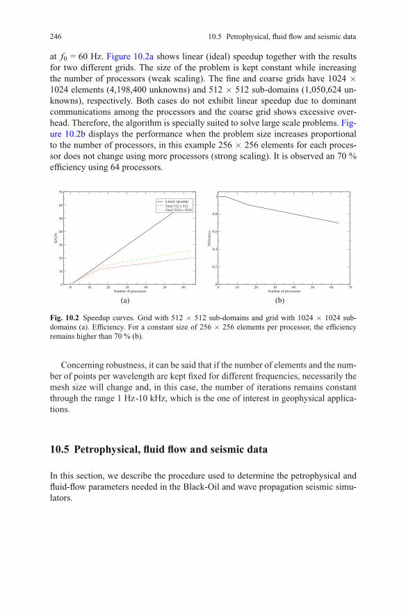
246
at f0 = 60 Hz. Figure 10.2a shows linear (ideal) speedup together with the resultsfor two different grids. The size of the problem is kept constant while increasingthe number of processors (weak scaling). The fine and coarse grids have 1024 ×1024 elements (4,198,400 unknowns) and 512 × 512 sub-domains (1,050,624 un-knowns), respectively. Both cases do not exhibit linear speedup due to dominantcommunications among the processors and the coarse grid shows excessive over-head. Therefore, the algorithm is specially suited to solve large scale problems. Fig-ure 10.2b displays the performance when the problem size increases proportionalto the number of processors, in this example 256 × 256 elements for each proces-sor does not change using more processors (strong scaling). It is observed an 70 %efficiency using 64 processors.
0 10 20 30 40 50 60Number of processors
0
10
20
30
40
50
60
70
S(N
,P)
Linear speedupGrid 512 x 512Grid 1024 x 1024
0 10 20 30 40 50 60 70Number of processors
0
0,2
0,4
0,6
0,8
1
Eff
icie
ncy
(a) (b)
Fig. 10.2 Speedup curves. Grid with 512 × 512 sub-domains and grid with 1024 × 1024 sub-domains (a). Efficiency. For a constant size of 256 × 256 elements per processor, the efficiencyremains higher than 70 % (b).
10.5 Petrophysical, fluid flow and seismic data
In this section, we describe the procedure used to determine the petrophysical andfluid-flow parameters needed in the Black-Oil and wave propagation seismic simu-lators.
10.5 Petrophysical, fluid flow and seismic data
Concerning robustness, it can be said that if the number of elements and the num-ber of points per wavelength are kept fixed for different frequencies, necessarily themesh size will change and, in this case, the number of iterations remains constantthrough the range 1 Hz-10 kHz, which is the one of interest in geophysical applica-tions.

247
10.5.1 A petrophysical model for the Utsira formation
The shaly sandstone model used here is that in [Carcione et al., 2000], where thetopology of the sandy and shaly mixture has been defined to obtain the petrophysicalproperties of the Utsira formation.
The pressure dependence of properties is based on the following relationshipbetween porosity and pore pressure:
(1−φc)Ks
(p(t)− pH) = φ0 −φ(t)+φc lnφ(t)φ0
, (10.28)
wherep(t) = Sbpb(t)+Sgpg(t)
is the pore pressure, φc is a critical porosity, φ0 = φ0(x,z) is the initial porosityat hydrostatic pore pressure pH and Ks is the bulk modulus of the solid grains[Carcione et al., 2003]. Porosity φ0 is assumed to have a fractal spatial distributionaround the average porosity 〈φ0〉, obtained from the neutron log by using standardmethods. The rock is formed with quartz (bulk modulus of 40 GPa) and clay (bulkmodulus of 15 GPa). Ks is computed as the arithmetic average of the Hashin Shtrik-man upper and lower bounds [Hashin and Shtrikman, 1963].
The relationship among horizontal permeability (κx1 ), porosity and clay content(C) is [Carcione et al., 2003]
1κx1(t)
=45(1−φ(t))2
φ(t)3
((1−C)2
R2q
+C2
R2c
), (10.29)
where Rq and Rc are the average radii of the sand and clay grains, respectively.Also, as permeability is anisotropic, we assume the following relationship be-
tween horizontal and vertical permeability [Carcione et al., 2003]
κx1(t)κx3(t)
=1− (1−0.3a)sin(πSb)a(1−0.5sin(πSb))
, (10.30)
where a is the permeability-anisotropy parameter.The bulk and shear moduli of the dry matrix, Km, μm are computed using the
Krief relation [Krief et al., 1990] as follows:
Km(t) = Ks(1−φ(t))A/(1−φ(t)). (10.31)
μm(t) = μs(1−φ(t))A/(1−φ(t)). (10.32)
Using the moduli Ks,μs,Km,μm, the porosity φ and permeabilities , , as well
[Peng and Robinson, 1976]), we determine the complex and frequency dependentLame coefficients λ (ω),μ(ω) as explained in Section 10.3.
κx3
as the fluids bulk moduli and viscosities (computed using the Peng-Robinson modelκx1 κx3
10 The macro-scale. Seismic monitoring of CO2 sequestration
,

248
Relative permeabilities and capillary pressure as functions of CO2 saturation arerepresented by the following potential models [Savioli and Bidner, 2005]:
Krg(Sg) = K∗rg
( Sg−Sgc1−Sgc−Sbc
)ng , (10.33)
Krb(Sg) = K∗rb
( 1−Sg−Sbc1−Sgc−Sbc
)nb , (10.34)
Pca(Sg) = P∗ca
( Sg−Sgc1−Sgc−Sbc
)nc , (10.35)
where ng, nb, nc determine the curvature of functions, K∗rg and K∗
rb are the maximumvalues of Krg, Krb and P∗
ca is a reference value of the capillary pressure Pca. Sgc andSbc are the saturations at which the CO2 and brine phases become mobile, respec-tively. The influence of capillary pressure on CO2 injection, storage and monitoringis analyzed in detail in [Santos et al., 2014b].
10.5.2 The Black Oil fluid model
The PVT data, Rs and Bb, can be expressed in terms of the equilibrium propertiesobtained from an equation of state as presented in [Hassanzadeh et al., 2008] and[Spycher and Pruess, 2005], i.e.,
Rs =ρSCb χg
ρSCg (1− χg)
, Bb =ρSCb
ρb(1−ωg),
where ρSCb and ρSC
g are the brine and CO2 molar densities at standard conditions,respectively, χg and ωg are the CO2 mole and mass fractions in the brine phase.The molar density is related to the mass density through the molecular weight.While the CO2 molecular weight (Mg) and mass density at standard conditions(ρSC
g ) are known, these properties for the brine phase must be estimated. The brinemolecular weight (Mb) is simply computed from the mole fractions χsalt of NaCland χH2O of H2O. The brine mass density at standard conditions, ρSC
b , is esti-mated following the Rowe and Chou correlation as given in formulas (B6)-(B14)of [Hassanzadeh et al., 2008] . Once ρSC
b is computed, ρb at reservoir conditions isobtained using the approach of Garcıa, as stated in [Hassanzadeh et al., 2008] . Thisapproach and the estimation of the CO2 mole and mass fractions in the brine phase,χg and ωg, are briefly explained in Appendix 10.9.
Finally, the viscosity, density and bulk modulus of CO2 are obtained from thePeng-Robinson equations [Peng and Robinson, 1976] as a function of temperatureand pore pressure.
10.5 Petrophysical, fluid flow and seismic data

249
10.6 Numerical simulations
To test the proposed methodology, we consider a model of the Utsira formationhaving 1.2 km in the x1-direction, 10 km in the x2-direction and 0.4 km in the x3-direction (top at 0.77 km and bottom at 1.17 km b.s.l.). The model and all propertiesare assumed to be uniform in the x2-direction. It is assumed that at the beginningof the simulation of CO2 injection the Utsira sandstone is fully saturated with brine(Sb = 1).
The pressure-temperature conditions are T = 31.7x3 + 3.4, where T is the tem-perature (in oC) and x3 is the depth (in km b.s.l.); pH = ρb gx3 is the hydrostaticpressure, with ρb = 1040 kg/m3 the density of brine and g the gravity constant.Within the formation, there are several mudstone layers which act as barriers to thevertical motion of the CO2 [Chadwick et al., 2009, Chadwick et al., 2010].
The initial porosity φ0 = φ0(x1,x3) at hydrostatic pore pressure for the Utsirasandstone (see eq.10.28) is assumed to have a fractal spatial distribution, obtainedas follows. First, we generate a fractal porosity distribution, based on the so-calledvon Karman self-similar correlation functions as defined in Chapter 7 (see 7.21).These models are widely used in the statistical characterization of heterogeneitiesfor different applications. The fractal porosity is obtained with the following relation
φ0(x1,x3) = 〈φ0〉+ f (x1,x3). (10.36)
In (10.36) 〈φ0〉 denotes the spatial average of φ0(x1,x3) and f (x1,x3) is a fractalfield representing the spatial fluctuation of φ0(x1,x3), for which the spectral densityis given in (7.21). For this application we use Euclidean dimension Ne = 2, fractaldimension D = 2.2 and 〈φ0〉 = 36.7 %. The correlation lengthCL in (7.21) was takento be 2 % of the domain size.
At the beginning of the simulation of the CO2 injection, the horizontal and verti-cal permeabilities were determined by using equations (10.29) and (10.30), consid-ering an anisotropy parameter a = 0.1 and a fixed clay content C = 6 %.
The minimum, average and maximum porosities obtained are 32.5 %, 36.7 % and38.3 %. The corresponding minimum, average and maximum vertical permeabilitiesare 0.1 D, 0.12 D and 0.145 D.
The mudstone layers are not completely sealed, having constant porosity 24 %and vertical permeability 0.033 D. Besides, they have openings, that give a pathfor the upward migration of CO2. The top and bottom of the Utsira formation haveconstant porosity 22 % and vertical permeability 0.02 D.
The initial porosity and vertical permeability fields can be observed in Figures10.3 and 10.4, respectively. Since before CO2 injection begins Sb = 1, it followsfrom (10.30) that initial horizontal permeability values are ten times those of theinitial vertical permeability.
10 The macro-scale. Seismic monitoring of CO2 sequestration

250
1.17
1.07
0.97
0.87
0.77
0 0.3 0.6 0.9 1.2
Depth (km)
Horizontal Distance (km)
0.2
0.22
0.24
0.26
0.28
0.3
0.32
0.34
0.36
0.38
0.4
porosity
Fig. 10.3 Initial porosity distribution before CO2 injection.
1.17
1.07
0.97
0.87
0.77
0 0.3 0.6 0.9 1.2
Depth (km)
Horizontal Distance (km)
0
20
40
60
80
100
120
140
160
Vertical permeability (mD)
Fig. 10.4 Vertical permeability distribution before CO2 injection.
10.6 Numerical simulations

251
10.6.1 CO2 injection
CO2 is injected during seven years in the Utsira formation at a constant flow rateof one million tons per year [Chadwick et al., 2010]. The injection is located atthe bottom of the formation: x1 = 0.6 km, x3 =1.082 km [Chadwick et al., 2005,Chadwick et al., 2009]. The simulation uses a mesh with equally-spaced blocksin each direction: nx1 = 300 in the x1-direction, nx2 = 5 in the x2-direction andnx3 = 400 in the x3-direction. Actually the model is 2.5D since the properties areuniform along the x2-direction, which has an extension of 10 km. It was verifiedthat taking larger extensions of the domain in the x2-direction did not change signif-icantly the CO2 saturation and pressure maps. Along the x2-direction, the third gridis used to locate the injection.
The flow parameter values in the relative permeability and capillary pressureformulas (10.33), (10.34) and (10.35) were chosen as follows: Sgc = 0.02, Sbc =0.12, ng = 1.15, nb = 2.5, nc = 4, K∗
rb = 0,95,K∗rg = 1,P∗
ca = 0.03 MPa.To satisfy the CFL stability condition due to IMPES formulation [Savioli and Bidner,
the time step value is 0.125 d. With this choice of the mesh and time step, theof the BOAST simulator satisfy the mass conservation condition.
Recall that the petrophysical properties of the formation are time dependent dueto the CO2 injection and consequently pore pressure increase (cf. (10.28), (10.29),(10.30)) but they change at a much slower rate than pressure and saturations. As aconsequence, we have two time scales, and we use a much larger time step to updatepetrophysical properties than to run the flow simulator. After performing a sensibil-ity analysis, in this numerical simulation we choose to update the petrophysicalproperties every year.
Figures 10.5, 10.6, 10.7 and 10.8 show 2-D vertical slices (corresponding tonx2 = 3) of the CO2 saturation fields after one, three, five and seven years of CO2 in-jection, respectively. In all the cases, CO2 accumulations below the mudstone layerscan be observed. As injection proceeds, part of the injected fluid migrates upwardsdue to the openings in the mudstone layers generating chimneys, and the verticalfluid flow is ruled by the vertical permeability. As CO2 saturation increases, verticalpermeability updated with equation (10.30) also increases, in particular in the mud-stone layers. This allows an increase in the CO2 upward motion across the layerswith the resulting low CO2 saturations levels observed between layers. As a conse-quence, CO2 chimneys become less defined as injection time increases, as it can beseen in these Figures.
A 2-D slice (at nx2 = 3) of the saturation dependent vertical permeability dis-tribution after seven years of CO2 injection is shown in Figure 10.9. Porosity andhorizontal permeability depending only on pressure suffer little changes and are notshown.
Capillary forces play an important role in multi-phase fluid flow, in particulargoverning diffusion effects. This fact can be observed in Figures 10.10 and 10.11displaying the difference between CO2 and brine pressure (capillary pressure) afterone and seven years of injection, respectively. As CO2 saturation increases and ac-
2005],results
10 The macro-scale. Seismic monitoring of CO2 sequestration

252
cumulates below the mudstone layers, capillary pressure increases and flow is moreaffected by capillary forces.
1.17
1.07
0.97
0.87
0.77
0 0.3 0.6 0.9 1.2
Depth (km)
Horizontal Distance (km)
0
0.1
0.2
0.3
0.4
0.5
0.6
0.7
CO2 saturation
Fig. 10.5 Spatial CO2 saturation distribution after one year of CO2 injection.
10.7 Seismic monitoring of CO2 injection
This Section describes the implementation of the iterative domain decompositionprocedure (10.26)-(10.27) to seismic monitor the CO2 injection.
10.7.1 Modeling mesoscopic-scale attenuation and dispersionusing time-harmonic experiments
The viscoelastic model needs the complex plane-wave and shear moduli. In the top,base and within the mudstone layers, the undrained bulk modulus Ku and the shearmodulus μ are computed using a Zener model as explained in Section 10.3 choosing
Q(1)Ku
= 100 at the central frequency of the source. Within the Utsira formation, theCO2-saturation dependent complex plane-wave and shear moduli, are determinedusing the time-harmonic compressibility tests described in Chapter 7. For this pur-
10.7 Seismic monitoring of CO2 injection

253
1.17
1.07
0.97
0.87
0.77
0 0.3 0.6 0.9 1.2
Depth (km)
Horizontal Distance (km)
0
0.1
0.2
0.3
0.4
0.5
0.6
0.7
0.8
CO2 saturation
Fig. 10.6 Spatial CO2 saturation distribution after three years of CO2 injection.
1.17
1.07
0.97
0.87
0.77
0 0.3 0.6 0.9 1.2
Depth (km)
Horizontal Distance (km)
0
0.1
0.2
0.3
0.4
0.5
0.6
0.7
0.8
CO2 saturation
Fig. 10.7 Spatial CO2 saturation distribution after five years of CO2 injection.
10 The macro-scale. Seismic monitoring of CO2 sequestration

254
1.17
1.07
0.97
0.87
0.77
0 0.3 0.6 0.9 1.2
Depth (km)
Horizontal Distance (km)
0
0.1
0.2
0.3
0.4
0.5
0.6
0.7
0.8
CO2 saturation
Fig. 10.8 Spatial CO2 saturation distribution after seven years of CO2 injection.
1.17
1.07
0.97
0.87
0.77
0 0.3 0.6 0.9 1.2
Depth (km)
Horizontal Distance (km)
0
500
1000
1500
2000
2500
Vertical permeability (mD)
Fig. 10.9 Vertical permeability distribution after seven years of CO2 injection.
10.7 Seismic monitoring of CO2 injection

255
1.17
1.07
0.97
0.87
0.77
0 0.3 0.6 0.9 1.2
Depth (km)
Horizontal Distance (km)
0
0.002
0.004
0.006
0.008
0.01
0.012
capillary pressure (MPa)
Fig. 10.10 Capillary pressure distribution after one year of CO2 injection.
1.17
1.07
0.97
0.87
0.77
0 0.3 0.6 0.9 1.2
Depth (km)
Horizontal Distance (km)
0
0.002
0.004
0.006
0.008
0.01
0.012
0.014
0.016
0.018
capillary pressure (MPa)
Fig. 10.11 Capillary pressure distribution after seven years of CO2 injection.
10 The macro-scale. Seismic monitoring of CO2 sequestration

256
pose a double-entry table of these moduli for 40 frequencies and 20 saturations isconstructed. Then, for a fixed frequency, the moduli for the CO2 saturation of eachcomputational cell are determined by an interpolation algorithm.
In order to compute each plane-wave modulus in the table, we consider severalrepresentative poroelastic samples for each saturation. The bulk and shear moduliand density of the solid grains composing the matrix of all representative sampleswere chosen to be Ks = 34 GPa , μs = 44GPa and ρs = 2100 Kg/m3, respectively.Porosity, permeability, bulk and shear modulus of the porous matrix were taken to befractal and computed in a similar fashion as for the flow simulator runs. In particular,since in permeability is anisotropic, we determined a saturation dependent effectivepermeability κe f f (Sb) defined as
κe f f (Sb) =(κx1κx3(Sb)
)1/2.
Note that κx3(Sb) is fractal, since is defined in (10.30) in terms of κx1 .The average properties of the fractal fields for porosity φ , horizontal permeability
κx1 , bulk modulus Km and shear modulus μm of the dry matrix, denoted by < ·, ·>are shown in Table 10.2.
These samples are assumed to be saturated with brine and CO2, with the fluidsdistribution in the form of irregular patches fully saturated with CO2 and zones fullysaturated with brine. No mixing forces are taken into account and the two fluids areassumed to occupy different mesoscopic regions of the model. The generation ofthese patchy brine-CO2 distributions was explained in Subsection 7.7.1. Table 10.3shows the properties of the saturant fluids (brine and CO2) used in the harmonicexperiments.
In order to generate the CO2 patches, we need to fix both the sample size andthe correlation length, as well as the stochastic parameters. The correlation lengthdetermines the maximum size for any CO2 bubble. Here we use square samples ofside length 80 cm and a correlation length of 20 cm; fractal dimension is D = 2.2.
Figure 10.12 show the CO2 patches generated for overall saturations of 5% (a)and 30 % (b).
For all fluid-saturated poroelastic samples, we perform a time-harmonic com-pressibility test. Each test allows to obtain the complex plane-wave modulus foreach saturation and for the 40 different frequencies used to generate the double-entry table.
On the other hand, the complex shear modulus was determined as indicated inSection 10.3.
Figure 10.13 displays fluid pressure maps at frequencies 2 Hz (a) and 60 Hz (b).Both maps correspond to patchy brine-gas distributions for overall CO2 saturationSg = 30 %. It can be observed that pressure is lower in zones of 100 % CO2 satu-ration, and pressure gradients at the boundaries of the CO2 bubbles are higher at 60Hz than at 2 Hz.
10.7 Seismic monitoring of CO2 injection

257
0
200
200
0 100 200
Vertical side length (cm)
Horizontal side length (cm)
0
200
200
0 100 200
Vertical side length (cm)
Horizontal side length (cm)
Fig. 10.12 Patchy brine-gas distributions for Sg = 5 % (a) and 30 % overall CO2 saturations (b).White zones correspond to 100 % gas saturation and black zones to 100 % brine saturation.
0
40
80
Vertical side length (cm)
Horizontal side length (cm) 0
0.1
0.2
0.3
0.4
0.5
0.6
0.7
0.8
Fluid Pressure (Pa)
0
40
80
Vertical side length (cm)
Horizontal side length (cm) 0
0.1
0.2
0.3
0.4
0.5
0.6
0.7
0.8
Fluid Pressure (Pa)
Fig. 10.13 Fluid pressure map at frequency 2 Hz (a) and 60 Hz (b), corresponding to the patchybrine-gas distributions for overall CO2 saturation Sg = 30 %.
Table 10.2 Average physical properties of the solid matrix used in the time-harmonic experiments
< φ > < Km > < μm > < κx1 >
0.36 2.0 GPa 1.9 GPa 1 Darcy
10 The macro-scale. Seismic monitoring of CO2 sequestration

258
Table 10.3 Physical properties of the saturant fluids used in the time-harmonic experiments
Kf ρ f η
Brine 2.25 GPa 1040 Kg/m3 0.0018 Pa · s
CO2 3.7×10⁷ Pa 700 Kg/m3 0.00026 Pa · s
10.7.2 Time-lapse seismics applied to monitor CO2 sequestration
1.17
1.07
0.97
0.87
0.77
0 0.3 0.6 0.9 1.2
Depth (km)
Horizontal Distance (km)
2100
2150
2200
2250
2300
2350
2400
2450
2500
2550
2600
P-wave phase velocity (m/s)
Fig. 10.14 P-wave phase velocity map before CO2 injection.
The capability of seismic monitoring to identify zones of CO2 accumulation andmigration is now analyzed.
With this purpose, we use 2-D slices of CO2 saturation and fluid pressure mapsobtained from the flow simulator to construct a 2-D model of the Utsira formation.The mesh is 600 cells in the x1-direction and 200 cells in the x3-direction.
The iterative procedure given in equations (10.26)-(10.27) is used to compute thetime Fourier transforms of the displacement vector for 200 equally spaced temporalfrequencies in the interval (0,200 Hz). The values of the iteration parameter matrixβ jk on the interfaces Γjk were taken to be of the form of the absorbing boundarycondition matrix B in (10.10), with the values of the compressional and shear phase
10.7 Seismic monitoring of CO2 injection

259
1.17
1.07
0.97
0.87
0.77
0 0.3 0.6 0.9 1.2
Depth (km)
Horizontal Distance (km)
1400
1600
1800
2000
2200
2400
2600
P-wave phase velocity (m/s)
Fig. 10.15 P-wave phase velocity map at 50 Hz after seven years of CO2 injection.
1.17
1.07
0.97
0.87
0.77
0 0.3 0.6 0.9 1.2
Depth (km)
Horizontal Distance (km)
550
600
650
700
750
800
850
900
950
1000
1050
1100
S-wave phase velocity (m/s)
Fig. 10.16 S-wave phase velocity map before CO2 injection.
10 The macro-scale. Seismic monitoring of CO2 sequestration

260
1.17
1.07
0.97
0.87
0.77
0 0.3 0.6 0.9 1.2
Depth (km)
Horizontal Distance (km)
600
800
1000
1200
1400
1600
1800
S-wave phase velocity (m/s)
Fig. 10.17 S-wave phase velocity map at 50 Hz after seven years of CO2 injection.
1.17
1.07
0.97
0.87
0.77
0 0.3 0.6 0.9 1.2
Depth (km)
Horizontal Distance (km)
0
100
200
300
400
500
600
P-wave quality factor
Fig. 10.18 Quality factor QP of compressional waves at 50 Hz after seven years of CO2 injection.
10.7 Seismic monitoring of CO2 injection

261
1.17
1.07
0.97
0.87
0.77
0 0.3 0.6 0.9 1.2
Depth (km)
Horizontal Distance (km)
30
40
50
60
70
80
90
100
110
120
S-wave quality factor
Fig. 10.19 Quality factor QS of shear waves at 50 Hz after seven years of CO2 injection.
velocities vp(ω) and vs(ω) defining β jk computed as averages of their values in theneighboring cells Ω j and Ωk.
The seismic source is a spatially localized plane wave of main frequency 60 Hzlocated at z = 772 m. A line of receivers is located at the same depth to record theFourier transforms of the vertical displacements. Then, a discrete inverse Fouriertransform is applied to obtain the data used for the synthetic seismograms.
The plane-wave simulation (a flat line of point sources at each grid point at thesurface) is a good approximation to the stack. We could compute the stack ex-plicitly by computing n common shots and then performing the (more expensive)standard processing sequence but the plane-wave method is a good approximation[Carcione et al., 1994].
Now, we proceed to compare the initial and perturbed velocity model in order toshow how the presence of the accumulation of CO2 below the mudstone layers andthe CO2 plume changes the seismic response of the formation, and, in particular, toaccurate reproduce the pushdown effect observed in real seismograms.
First we analyze the effect of CO2 injection on the phase velocity and qualityfactors of compressional and shear waves.
Figures 10.14 and 10.15 display the spatial distribution of the compressionalwave phase velocity (vP) before injection and at 50 Hz after seven years of injection,while Figures 10.16 and 10.17 show the corresponding maps for shear waves.
Also, Figures 10.18 and 10.19 show maps of the quality factors QP and QS at 50Hz after seven years of injection, respectively.
10 The macro-scale. Seismic monitoring of CO2 sequestration

262
0
0.1
0.2
0.3
0.4
Tim
e (s
)
200 400 600 800 1000Distance (m)
Fig. 10.20 Synthetic seismogram before CO2 injection.
It is observed a noticeable decrease in phase velocity and quality factors for bothwaves in zones of CO2 accumulation. These strong changes in velocities and atten-uation induce delays and attenuation in the waves recorded at the top of the model,to be observed in the next Figures. These Figures show the synthetic seismograms(seismic sections) obtained measuring the vertical component of the displacementvector on a line of receivers at the top of the model.
Figures 10.20, 10.21 10.22, 10.23 and 10.24 display migrated seismic sectionsbefore CO2 injection and after one, three, five and seven years of CO2 injectionassociated with the CO2 saturations shown in Figures 10.5, 10.6, 10.7 and 10.8respectively.
A standard f -k filter is used to eliminate some spurious reflections from the artifi-cial boundaries of the computational mesh, since the absorbing boundary conditionsused are only first order and can not eliminate all undesired boundary reflections.
The reflections seen in those seismograms show the progressive increment inCO2 accumulations below the mudstone layers as injection proceeds. In particular,
10.7 Seismic monitoring of CO2 injection

263
0
0.1
0.2
0.3
0.4
Tim
e (s
)
200 400 600 800 1000Distance (m)
Fig. 10.21 Synthetic seismogram after one year of CO2 injection.
the pushdown effect observed in the real seismograms [Chadwick et al., 2009] dueto CO2 accumulations, as shown in the Figure 10.25, is clearly observed.
Summarizing, the combined use of multi-phase fluid-flow and viscoelastic wavepropagation simulators defines a methodology that becomes an important tool tomonitor the migration and dispersal of the CO2 plume, in order to analyze storageintegrity and to make long term predictions.
10.8 Appendix 1. IMPES solution for Black-Oil formulation
The IMPES technique combines the flow equations (10.6)- (10.7) to obtain a singlepressure equation. In this way, equation (10.6) multiplied by Bg and equation (10.7)multiplied by (Bb−RsBg) are added. The right-hand side of the combined equationresults,
10 The macro-scale. Seismic monitoring of CO2 sequestration

264
0
0.1
0.2
0.3
0.4
Tim
e (s
)
200 400 600 800 1000Distance (m)
Fig. 10.22 Synthetic seismogram after three years of CO2 injection.
Bg
∂[φ(SgBg
+RsSbBb
)]∂ t
+(Bb−RsBg)∂[φSbBb
]∂ t
. (10.37)
Using the chain rule to expand the time derivatives, and after some algebraicmanipulations, the expression in 10.37 becomes:
φ[ 1
φdφdpb
+Sg
(− 1Bg
dBg
dpb
)+Sb
(− 1Bb
dBb
dpb+
Bg
Bb
dRs
dpb
)]∂ pb∂ t
,
where all time derivatives of saturation have disappeared.Defining the compressibilities as
10.8 Appendix 1. IMPES solution for Black-Oil formulation

265
0
0.1
0.2
0.3
0.4
Tim
e (s
)
200 400 600 800 1000Distance (m)
Fig. 10.23 Synthetic seismogram after five years of CO2 injection.
Formation compressibility: c f =1φ
dφdpb
,
Gas compressibility: cg =− 1Bg
dBg
dpb,
Brine compressibility: cb =− 1Bb
dBb
dpb+
Bg
Bb
dRs
dpb,
Total compressibility: ct = c f +Sgcg+Sbcb,
the following simply expression is obtained for the right-hand side of the combinedequation,
φct∂ pb∂ t
.
10 The macro-scale. Seismic monitoring of CO2 sequestration

266
0
0.1
0.2
0.3
0.4
Tim
e (s
)
200 400 600 800 1000Distance (m)
Fig. 10.24 Synthetic seismogram after seven years of CO2 injection.
Finally, replacing pg by pb+PC(Sb) in the left side of the combined equation,the pressure equation (10.8) is obtained.
10.9 Appendix 2. Estimation of brine density and CO2 mole andmass fractions in the brine phase
The brine mass density at reservoir conditions is estimate using the approach ofGarcıa [Hassanzadeh et al., 2008] as follows,
ρb =1+(Mg/Mb)(χg/(1− χg))
(Vm/Mb)(χg/(1− χg))+1/ρSCb
,
10.9 Appendix 2. Estimation of brine density and CO2 mole and mass fractions...

267
Fig. 10.25 Real seismograms showing the pushdown effect (after [Chadwick et al., 2009]).
where Mg, Mb are the CO2 and brine molecular weights, respectively; χg is the CO2
mole fraction in the brine phase; ρSCb is the brine mass density at standard conditions
and Vm is a partial molar volume, computed as a function of temperature T (oC) asin formula (21) of [Hassanzadeh et al., 2008]:
Vm = 37.51−9.585×10⁻²T +8.74×10⁻⁴T 2 −5.044×10⁻⁷T 3.
To determine χg, we apply the following relationship
χg =mg
mg+55.508+νms,
where mg is the molality of CO2 in saline water, ms is the salt molality and ν is thestoichiometric number of ions in the dissolved salt. In order to compute mg we use
mg =mog
γ∗g,
where mog is the molality of CO2 in pure water and γ∗g the activity coefficient.
To obtain mog for each pressure and temperature, we solve iteratively the thermo-
dynamic nonlinear equations (B1)-(B5) in [Hassanzadeh et al., 2008]. These equa-
10 The macro-scale. Seismic monitoring of CO2 sequestration

268
tions involve H2O and CO2 molar volumes, fugacities and activity coefficients. TheCO2 molar volume is computed using the Peng-Robinson model [Peng and Robinson,
Also, γ∗g is obtained using the Rumpf model, as stated in equation (A6) in& Pruess [Spycher and Pruess, 2005].
Once χg is computed, the CO2 mass fraction in the aqueous phase ωg is obtainedfrom the relation:
ωg = χgMg
Maq.
Here Maq is the aqueous molecular weight, given by
Maq = χgMg+ χH2OMH2O+ χsaltMsalt .
1976].Spycher
10.9 Appendix 2. Estimation of brine density and CO2 mole and mass fractions...

Chapter 11
Wave propagation in partially frozen porousmedia
Abstract The propagation of waves in a fluid-saturated poroelastic medium whichmatrix is composed of two weakly coupled solids is simulated using an iterativefinite element domain decomposition algorithm. The equations of motion are for-mulated in the space-frequency domain including dissipation in the solid matrix andfrequency correction factors in the mass and viscous coupling coefficients. First or-der absorbing boundary conditions are employed at the artificial boundaries of thecomputational domain. The algorithm is applied to simulate wave propagation in asample of partially frozen Berea sandstone at ultrasonic frequencies.
11.1 Introduction
The propagation of waves in a three-phase porous medium composed of a fluid andtwo weakly-coupled porous solids is simulated using a finite element (FE) domaindecomposition procedure. The equations governing the propagation of waves in thistype of multiphase system were presented in Chapter 4.
The FE method is formulated in the space-frequency domain and includes solidmatrix dissipation using the linear viscoelastic model defined in (1.122)-(1.123) andfrequency dependent mass and viscous coupling coefficients.
Numerical simulation of waves in porous media is computationally expensivedue to the large number of degrees of freedom needed to calculate wave fields ac-curately; the use of a domain decomposition iteration is a convenient approach toovercome this difficulty. The FE domain decomposition procedure used here is sim-ilar to that used in Chapter 10 (cf. (10.26)–(10.27)). The displacement vector in thesolid phases is approximated using the non-conforming finite element space MC
h
defined in Chapter 6 in (6.68). The vector displacement in the fluid phase is approx-imated using the finite element space V h defined in (6.52).
The numerical procedure is used for the simulation of waves in a sample of wa-ter saturated partially frozen Berea sandstone. The wave fields are generated by
© Springer International Publishing AG 2016
in Geosystems Mathematics and Computing, DOI 10.1007/978-3-319-48457-0_11
269J.E. Santos, P.M. Gauzellino, Numerical Simulation in Applied Geophysics, Lecture Notes

270
a point source at ultrasonic frequencies. The snapshots show the generated wavefields, where the events associated with the different types of waves can be clearlyobserved.
11.2 The finite element domain decomposition iteration
Consider the solution of the equations of motion (4.20)-(4.22) in a rectangular poro-viscoelastic domain Ω in the (x1,x3)–plane using a domain decomposition proce-dure. We use the notation given in Chapter 4 to refer to displacements, stresses andother variables defining the differential model for this three-phase composite sys-tem.
Let T h be a non-overlapping partition of Ω into rectangles Ω j of diameterbounded by h such that Ω = ∪J
j=1Ω j. Set Γj = ∂Ω ∩ ∂Ω j, Γjk = ∂Ω j ∩ ∂Ωk, anddenote by ξ j and ξ jk the midpoints of Γj and Γjk, respectively. Let us denote by ν jk
the unit outer normal on Γjk from Ω j to Ωk and by ν j the unit outer normal to Γj.Let χ j and χ jk be two unit tangents on Γj and Γjk so that ν j,χ j and ν jk,χ jk areorthonormal systems on Γj and Γjk, respectively.
Let u j =(u(1)j ,u(2)j ,u(3)j
)denote the restriction of u to the set Ω j and set
G j(u j) =
(σ (1,T )(u j)ν j ·ν j,σ (1,T )(u j)ν j · χ j, p f (u j),
σ (3,T )(u j)ν j ·ν j,σ (3,T )(u j)ν j · χ j
), (x1,x3) ∈ Γj,
G jk(u j) =
(σ (1,T )(u j)ν jk ·ν jk,σ (1,T )(u j)ν jk · χ jk, p f (u j),
σ (3,T )(u j)ν jk ·ν jk,σ (3,T )(u j)ν jk · χ jk
), (x1,x3) ∈ Γjk,
ΠΓj(u j) =(u(1)j ·ν j,u
(1)j · χ j,u
(2)j ·ν j,u
(3)j ·ν j,u
(3)j · χ j
), (x1,x3) ∈ Γj,
ΠΓjk(u j) =(u(1)j ·ν jk,u
(1)j · χ jk,u
(2)j ·ν jk,u
(3)j ·ν jk,u
(3)j · χ jk
), (x1,x3) ∈ Γjk.
If Ω j has a part Γj of its boundary contained in ∂Ω , we impose the absorbing bound-ary condition (see [Sheen, 1993])
−G j(u j) = iωBpΠΓj(u j), (x1,x3) ∈ Γj, (11.1)
where the symmetric positive definite matrix Bp is given in (5.83).Furthermore, as in (10.22) for the case of a viscoelastic medium, at the interior
interface Γjk we use the Robin transmission boundary conditions:
G jk(u j)+ iωβ jkΠΓjk(u j) = Gk j(uk)− iωβ jkΠΓk j(uk), (x1,x3) ∈ Γjk ⊂ ∂Ω j, (11.2)
11.2 The finite element domain decomposition iteration

271
Gk j(uk)+ iωβ jkΠΓk j(uk) = G jk(u j)− iωβ jkΠΓjk(u j), (x1,x3) ∈ Γjk ⊂ ∂Ωk. (11.3)
Here β jk is a positive definite matrix function defined on the interior boundaries Γjk.The Robin transmission conditions (11.2)–(11.3) impose the continuity of the soliddisplacements, the normal component of the fluid displacements and the generalizedstresses at the interior interfaces Γjk.
Next we introduce a set of Lagrange multipliers ηjk=(η1,νjk ,η1,χ
jk ,−η fjk,η
3,νjk ,η3,χ
jk )
associated with the values of the generalized stresses G jk at the mid points ξ jk of Γjk
in the sense that η jk ∼ G jk(u j)(ξ jk).The Lagrange multipliers η jk belong to the following space of functions defined
on the interior interfaces Γjk:
Lh =
η :η |Γjk = η jk ∈ [P0(Γjk)]5 = L
hjk, ∀ j,k
,
where P0(Γjk) denotes the constant functions on Γjk.Let us proceed to state a domain decomposition iteration using a variational for-
mulation.The local finite element space MC
hj defined in (6.67) (for n=2) is used to repre-
sent the displacement vectors in the two solid phases while the space V hj defined in
(6.53) is employed to represent the fluid phase.The domain decomposition iteration is defined as follows:
given(U0
j =(U(1),0
j ,U(2),0j ,U(3),0
j
),η0
jk
)∈MC
hj×V h
j ×MChj×L h
jk for all j, for
n = 1,2,3, · · · , find(Un
j =(U(1),n
j ,U(2),nj ,U(3),n
j
),ηn
jk
)∈ MC
hj ×V h
j ×MChj ×
L hjk such that
−ω2 (A Un
j , v)j+∑
pq
(σ (1,T )pq (Un
j), εpq(v1)
)j
−(p f (Un
j), ∇ ·v2)
j+∑
pq
(σ (3,T )pq (Un
j), εpq(v3)
)j
(11.4)
+
⟨⟨iωBpΠΓj(U
nj), ΠΓj(v)
⟩⟩Γj
+∑k
⟨⟨iωβ jkΠΓjk(U
nj),ΠΓjk(v)
⟩⟩Γjk
=(f(1), v1
)j+(f( f ), v2
)j+(f(3), v3
)j
−∑k
⟨⟨iωβ jkΠΓk j(U
n−1k ), ΠΓjk(v)
⟩⟩Γjk
−∑k
⟨⟨(−ηn−1k j ,ΠΓjk(v)
⟩⟩Γjk
,
v= (v1,v2,v3) ∈ MChj ×V
hj ×MC
hj ×L
hjk,
ην ,njk = ην ,n−1
k j − iωβ jk
(ΠΓjk(U
nj)+ΠΓk j(U
n−1k )
)(ξ jk). (11.5)
where
11 Wave propagation in partially frozen porous media

272
A =
⎡⎣m11I m12I m13Im12I m22I m23Im13I m23I m33I
⎤⎦ ,I denotes the identity matrix in R3×3 and the mass coefficients mi j = mi j(ω) aredefined in (4.28).
In (11.4) 〈〈u,v〉〉Γ denotes the approximation of the L2(Γ ) inner product < ·, ·>Γby the mid–point quadrature.
Equation (11.5), used to update the Lagrange multipliers, is obtained directlyfrom (11.2) evaluated at the mid point ξ jk. Equation (11.4) yields a 20× 20 linearsystem of equations for the degrees of freedom associated with the vector displace-ments of the three phases on each sub-domain Ω j at the n−iteration level. Theiteration (11.4)–(11.5) is a Jacobi–type iteration. A twice as fast iteration may alsobe defined by using a red–black type iteration (see Table 10.1).
The iteration matrix β jk is chosen to have the same form of the matrix Bp in(11.1). The space–time solution is obtained by solving (11.4)–(11.5) for a finitenumber of frequencies and using an approximate inverse Fourier transform. Thedefinition of the iteration (11.4)–(11.5) can be extended to the case of larger sub-domains Ω j, as explained in Chapter 10.
11.3 A numerical example in the ultrasonic range of frequencies
We consider wave propagation in a square sample Ω of partially frozen Berea sand-stone of side length L= 3 cm. Set
Ω = Ω1 ∪Ω2 ∪Ω3
with Ω1,Ω2 and Ω3 denoting the Berea, water and ice portions of Ω . If Vi denotesthe volume of the i-portion of Ω , the ice content S′3 in the pores is determined bythe relation
S′3 =V3
V1 +V2.
The sample is assumed to have an interior horizontal plane interface Γi at x3 = 1.5cm defined by a change in ice content in the pores.
The material properties of the system, taken from [Carcione and Seriani, 1998,Carcione and Tinivella, 2000a] are given in Table 11.1. In this case the indices 1and 3 correspond to the sandstone and ice properties, respectively. The mesh is anuniform partition of Ω into squares of side length h= L/nx1 , with nx1 = nx3 = 200.
The source function (f1, f f , f3) is a compressional and shear point source locatedat (xs,zs) = (1.5 cm, 1.0 cm) applied to the solid and fluid phases, with a band limitedspectrum of central frequency equal to 500 kHz.
11.3 A numerical example in the ultrasonic range of frequencies
The absolute porosity of the sandstone is φa = φ chosensuch that the ice content S
′3 in the pores changes at the interface Γ from 66 percent
in the upper layer to 33 percent in the lower layer.
0.3, with the water content

273
For the calculation of the elastic coefficients we need values for the bulk andshear modulus of the two solid dry frames, denoted by Ks1,m,Ks3,m, μs1,m andμs3,m, respectively. Following [Leclaire et al., 1994, Carcione and Tinivella, 2000a]and [Santos et al., 2004a] it is assumed that Ks1,m= 14.4 GPa and that the modu-lus μs1,m, μs3,m and Ks3,m can be computed using a percolation-type model us-
ing the relations (4.37) where μ(max)s1,m ,μ(max)
s3,m and K(max)s3,m are computed using the
Kuster and Toksoz’s model[Kuster and Toksoz, 1974], taking the known values ofKs1,μs1,Ks3,μs3 for the background medium with inclusions of air, with propertiesKa,μa. The moduli μ0
s1,m, μ0s3,m and K0
s3,m are appropriate reference values. Here wetake
μ0s1,m = 13.3 GPa, K0
s3,m = μ0s3,m = 0.
The viscoelastic behaviour of the material is modeled using the parameters t1,M =10−1ms, t2,M = 109ms (see notation in Appendix 1.9) to make the moduli M =KG1,KG3,μ1,μ3,μ13,B3 complex and frequency dependent. The mean quality fac-tors are taken to be QKG1 = QKG3 = Qμ1 = Qμ3 = 100 and Qμ13 = QB3 = 200. Thevalue of the Kozeny-Carman constant was taken to be 5 [Hovem and Ingram, 1979].
Table 11.1 Material properties of the partially frozen sandstone model
Solid grain bulk modulus, Ks1 38.7 GPashear modulus, μs1 39.6 GPadensity, ρ1 2650 kg/m3
permeability κ1,0 1.07 10−13 m2
Ice bulk modulus, Ks3 8.58 GPashear modulus, μs3 3.32 GPadensity, ρ3 920 kg/m3
permeability κ3,0 5 10−4 m2
Water bulk modulus, Kf 2.25 GPadensity, ρ2 1000 kg/m3
viscosity, η 1.798 cPAir bulk modulus, Ka 1.5 10−4 GPa
shear modulus, μa 0 GPa
Table 11.2 displays values of the phase velocity and attenuation factors at 500kHz for the five different types of waves for the two–layer model used in this exper-iment.
The following Figures present snapshots of the wave fields for this experiment,generated after solving (11.4)–(11.5) for 110 equally spaced temporal frequenciesin the interval (0,1MHz). To understand and identify more clearly the various kindsof waves propagating in the partially frozen sandstone we also show snapshots ofthe curl and divergence of the displacements of the three phases, i.e., the rock frame,the ice and the fluid.
Figures 11.1, 11.2 and 11.3 show respectively snapshots of the vertical compo-nent of the particle velocity of the three phases at t = 0.005 ms where we can observe
11 Wave propagation in partially frozen porous media

274
Table 11.2 Wave speeds and attenuation factors for all waves at frequency 500 kHz
Ice content 0.66 Ice content 0.33Wave Phase velocity (km/s) Attenuation (dB) Phase velocity (Km/s) Attenuation (dB)Fast P1 wave 4.08 0.35 3.90 0.47Slow P2 wave 1.37 5.20 1.05 7.88Slow P3 wave 0.22 30.0 0.22 6.70Fast S1 wave 2.72 0.58 2.58 0.74Slow S2 wave 0.57 2.45 0.22 1.04
that after arriving at the interface Γi, the direct P1 and P2 waves have generated re-flected and transmitted fast and slow shear and compressional waves. In particularthe P2 wave generated at the source has arrived at Γi at t = 0.0035 and has generatedreflected and transmitted fast and slow compressional and shear waves. The shortwavelength located near the source corresponds to the slow shear wave generatedby the source.
Figures 11.4, 11.5 and 11.6 show respectively snapshots of the vertical compo-nent of the particle velocity of the three phases at t = 0.01 ms. In Figure 11.4 canbe seen a fast transmitted P1 wavefront arriving at the top boundary and a slow P2wavefront above Γi, that is clearly identified by observing the snapshot of the diver-gence of the ice phase at at t = 0.01 ms shown in Figure 11.7. In the same Figure,below Γi we see a reflected P2 wavefront which front is passing through the sourcelocation, and a reflected P1 wavefront arriving at the bottom boundary. These last towavefronts are also clearly identified in Figure 11.7.
The other wavefronts seen in Figures 11.4, 11.5 and 11.6 correspond to shearwaves. The strong wavefront at the center in these 3 Figures is a slow shear wavegenerated at the source that is arriving at the interface Γi generating fast and slowcompressional and shear waves. Figure 11.8 shows a slow wave shear wavefrontarriving at Γi and generating slow reflected and transmitted slow shear waves, iden-tified as slow waves because of their short wavelengths.
Finally, Figures 11.9, 11.10 and 11.11 display snapshots of the three phases at t =0.02 ms. There are fast and slow compressional and shear waves above and belowΓi. Looking at the divergence of the ice phase in Figure 11.12 and the correspondingvertical displacement in Figure 11.10 we can identify a slow transmitted P2 waveabove Γi and a fast transmitted P1 wave of larger wavelength at the top of the Figure.The strong wavefront below Γi is a fast transmitted P1 wave travelling towards thebottom boundary. Concerning shear wavefronts, by observing the curl of the icephase in Figure 11.13, we can identify in Figure 11.10 a transmitted slow shearwavefront above Γi and two reflected slow shear wavefronts below Γi. The centerof the wavefront below and closer to Γi is passing through the source location, andthe other slow shear wavefront below Γi is arriving at the bottom boundary. This lastslow shear wavefront is arriving at the bottom boundary before the fast reflected fastP1 wave observed in Figure 11.12.
11.3 A numerical example in the ultrasonic range of frequencies

275
0
1.5
3.
0 1.5 3.
Vertical side length (cm)
Horizontal side length (cm)
Fig. 11.1 Ice content interface. Vertical component of the velocity of the rock frame at t = 0.005ms.
0
1.5
3.
0 1.5 3.
Vertical side length (cm)
Horizontal side length (cm)
Fig. 11.2 Ice content interface. Vertical component of the velocity of the ice frame at t = 0.005ms.
11 Wave propagation in partially frozen porous media

276
0
1.5
3.
0 1.5 3.
Vertical side length (cm)
Horizontal side length (cm)
Fig. 11.3 Ice content interface. Vertical component of the velocity of the fluid at t = 0.005 ms.The relative amplitudes between the snapshots in Figures 11.1, 11.2 and 11.3 is 1/196.3/4.15.
0
1.5
3.
0 1.5 3.
Vertical side length (cm)
Horizontal side length (cm)
Fig. 11.4 Ice content interface. Vertical component of the velocity of the rock frame at t = 0.01ms.
11.3 A numerical example in the ultrasonic range of frequencies

277
0
1.5
3.
0 1.5 3.
Vertical side length (cm)
Horizontal side length (cm)
Fig. 11.5 Ice content interface. Vertical component of the velocity of the ice frame at t = 0.01 ms.
0
1.5
3.
0 1.5 3.
Vertical side length (cm)
Horizontal side length (cm)
Fig. 11.6 Ice content interface. Vertical component of the velocity of the fluid at t = 0.01 ms. Therelative amplitudes between the snapshots in Figures 11.4, 11.5 and 11.6 is 1/154.2/3.26.
11 Wave propagation in partially frozen porous media

278
0
1.5
3.
0 1.5 3.
Vertical side length (cm)
Horizontal side length (cm)
Fig. 11.7 Ice content interface. Divergence of the displacement of the solid phase 3 at t = 0.01 ms.
0
1.5
3.
0 1.5 3.
Vertical side length (cm)
Horizontal side length (cm)
Fig. 11.8 Ice content interface. Curl of the displacement of the solid phase 3 at t = 0.01 ms.
11.3 A numerical example in the ultrasonic range of frequencies

279
0
1.5
3.
0 1.5 3.
Vertical side length (cm)
Horizontal side length (cm)
Fig. 11.9 Ice content interface. Vertical component of the velocity of the rock frame at t = 0.02ms.
0
1.5
3.
0 1.5 3.
Vertical side length (cm)
Horizontal side length (cm)
Fig. 11.10 Ice content interface. Vertical component of the velocity of the ice frame at t = 0.02ms.
11 Wave propagation in partially frozen porous media

280
0
1.5
3.
0 1.5 3.
Vertical side length (cm)
Horizontal side length (cm)
Fig. 11.11 Ice content interface. Vertical component of the velocity of the fluid at t = 0.02 ms.The relative amplitudes between the snapshots in Figures 11.9, 11.10 and 11.11 is 1/157.2/3.4.
0
1.5
3.
0 1.5 3.
Vertical side length (cm)
Horizontal side length (cm)
Fig. 11.12 Ice content interface. Divergence of the displacement of the solid phase 3 at t = 0.02ms.
11.3 A numerical example in the ultrasonic range of frequencies

281
0
1.5
3.
0 1.5 3.
Vertical side length (cm)
Horizontal side length (cm)
Fig. 11.13 Ice content interface. Curl of the displacement of the solid phase 3 at t = 0.02 ms.
11 Wave propagation in partially frozen porous media

Chapter 12
The macro-scale. Wave propagation intransversely isotropic media
Abstract The propagation of seismic waves in a fluid-saturated poroelastic mediumcontaining a dense set of aligned fractures is simulated using a non-conformingfinite element (FE) domain decomposition procedure. The macroscopic propertiesof this fractured medium are determined using the set of time-harmonic up-scalingexperiments developed in Chapter 8, with the fractures modeled as extremely thin,highly permeable and compliant porous layers. This approach yields a complex andfrequency dependent stiffness matrix defining an equivalent transversely isotropicviscoelastic (TIV) medium at the macro-scale. The FE procedure to simulate wavepropagation in TIV media is completely analogous to the one explained in Chapter10 for isotropic viscoelastic media. Fracture induced anisotropy and the influenceof different fluids filling the fractures are analyzed in the numerical examples.
12.1 Introduction
In geophysical prospecting is of relevant interest the characterization of fracturedporous media in reservoir environment, aquifers and other formations. In this Chap-ter we use the time-harmonic up-scaling experiments described in Chapters 8 todetermine the macroscopic properties of this kind of media, with fractures modeledas highly permeable and compliant thin poroelastic layers.
Under simplifying hypothesis, it has been shown in Chapters 8 that a porousmedium containing a dense set of aligned fractures behaves as an effective trans-versely isotropic and viscoelastic (TIV) medium. This approach determines thecomplex and frequency dependent TIV coefficients for the general case of highlyheterogeneous saturant fluids and fracture and background petrophysical properties.We emphasize that in this type of medium P and S seismic waves show frequencyand angular variations of velocity and attenuation. These anisotropic behaviour isdue to the mesoscopic loss mechanism caused by slow (diffusion) Biot waves gen-
© Springer International Publishing AG 2016
in Geosystems Mathematics and Computing, DOI 10.1007/978-3-319-48457-0_12
283J.E. Santos, P.M. Gauzellino, Numerical Simulation in Applied Geophysics, Lecture Notes

12.2 Properties of the equivalent TIV medium
Application of numerical simulation to determine rock properties is called Com-putational Rock Physics. In this context, the time-harmonic up-scaling proceduresoffer an alternative to laboratory measurements with the advantages of being in-expensive, repeatable and essentially free from experimental errors. Moreover, thenumerical experiments may be run using alternative models of the rock and fluidproperties.
Since at the macro-scale the wavelength of the travelling waves is much largerthan the distance between fractures, a dense set of parallel plane fractures in a fluid-saturated poroelastic medium behaves as a equivalent TIV medium, and the stiffnesscoefficients (pi j with 1 ≤ i, j ≤ 6) can be determined as explained in Chapter 8.
In the examples shown here, we consider a fluid-saturated porous material withfractures modeled as thin layers of aperture 1 cm and high and low fracture intensityor frequency (fractures per meter): 20 and 2 fractures per meter, respectively.
These representative samples are characterized by the values of the material prop-erties given in Table 12.1. The Krief model, whose expression is given in (8.41), isused to obtain the dry bulk and shear modulus of the background and fractures. Per-meabilities are calculated using the expression (8.42) with rg=20 μm as the averageradius of the grains.
Using relations given in Appendix 8.9, we calculated the energy velocities anddissipation coefficients using the pi j(ω) coefficients for the TIV media with verticalsymmetry axis (VTIV).
Figure 12.1 shows polar representation of the energy velocities, where qP is thequasi-compressional wave, qSV is the quasi-shear wave and SH is the pure cross-plane shear wave. The curves correspond to a frequency of 30 Hz. In these cases,the background is saturated by brine and gas fills the fractures. When comparingthe above mentioned fracture intensities, it is clearly observed that a higher fracturefrequency induces a higher degree of anisotropy.
284
erated at mesoscopic-scale heterogeneities, as explained in Chapter 7; (see also[Biot, 1956a, Biot, 1962, White et al., 1975, White, 1975, Pride et al., 2004]).
The numerical up-scaling experiments developed in Chapter 8 determine the fivecomplex and frequency dependent stiffnesses coefficients characterizing the equiv-alent TIV medium at the macro-scale.
In the examples, we first characterize the equivalent TIV medium showing theenergy velocities and attenuation coeffcients for different fracture intensities anddifferent fluids filling the fractures.
Next, the propagation of seismic waves at the macroscale is simulated using anon-conforming FE domain decomposition iteration. This numerical strategy hasalready been used in Chapter 10 for 2-D isotropic viscoelastic media and applied towave propagation in 2-D and 3-D media and to different rheological equations in[Gauzellino et al., 2001, Santos et al., 2004b, Gauzellino et al., 2014].
12.2 Properties of the equivalent TIV medium

12 The macro-scale. Wave propagation in transversely isotropic media 285
Table 12.1 Material properties of the background, fractures and saturant fluids
Background bulk modulus, Ks 37. GPashear modulus, μs 44. GPagrain density, ρs 2650 kg/m3
dry bulk modulus, Km 1.17 GPadry shear modulus, μ 1.4 GPaporosity, φ 0.25permeability, κ 2.5 10−13 m2
tortuosity, S 2.8
Fractures bulk modulus, Ks 37. GPadry bulk modulus, μm 4.55 GPadry shear modulus, μm 0.69 GPaporosity, φ 0.5permeability κ 2.5 10−10 m2
tortuosity, S 2.8
Brine bulk modulus, Kw 2.25 GPadensity, ρw 1040 kg/cm3
viscosity, ηw 0.0018 Pa · s
Oil bulk modulus, Ko 0.57 GPadensity, ρo 700 kg/cm3
viscosity, ηo 0.004 Pa · s
Gas bulk modulus, Kg 25. 106 Padensity, ρg 500 kg/m3
viscosity, ηg 0.00002 Pa · s
Vex (km/s)
Vez
(km
/s)
1
2
3
4
30
60
90
0
qPqSVSH
1 2 3 4Vex (km/s)
Vez
(km
/s)
1
2
3
4
30
60
90
0
qPqSVSH
1 2 3 4
(a) (b)
Fig. 12.1 Polar representation of the qP, qSV and SH energy velocity vectors at 30 Hz for gas-filledfractures, (a) High fracture intensity, and (b) low fracture intensity.

286
The influence of different fluids filling the fracture is illustrated in Figure 12.2.In this case, the qP, qSV and SH energy velocities at 30 Hz are shown together withtheir respective quality factors for oil saturated fractures. When comparing Figure12.1a with Figure 12.2a, it is observed that qP velocities are higher for oil than forgas saturated fractures. Concerning attenuation, energy losses for qSV waves aremuch higher for angles between 30 and 60 degrees. Notice that for qP waves dis-sipation anisotropy is much important for waves travelling in the direction incidentnormal to the fracture planes and the quality factor,Q, is great on angles close to 45degrees.
Vex (km/s)
Vez
(km
/s)
1
2
3
4
30
60
90
0
qPqSVSH
1 3 421000/Q(X)
1000
/Q(Z
)
1
2
3
30
60
90
0
qPqSV
1 2 3
(a) (b)
Fig. 12.2 Polar representation of the qP, qSV and SH energy velocity vectors (a), and the qualityfactors (b) at 30 Hz for oil-filled fractures and high fracture intensity.
The up-scaling time-harmonic experiments performed at the meso-scale allowsto obtain the stiffness matrix P = (pIJ) in (8.9) determining the equivalent TIVmedium at the macroscale. For a frequency of 30 Hz with high fracture intensityand gas saturated fractures the stiffness matrix P is
P=
⎛⎜⎜⎜⎜⎝(24.35,0.07) (1.89,0.07) (0.66,0.01) 0 0 0(1.89,0.07) (24.35,0.07) 0.66,0.01 0 0 0(0.66,0.01) 0.66,0.01 (6.45,0.002) 0 0 0
0 0 0 (2.87,5.10−15) 0 00 0 0 0 (2.87,5.10−15) 00 0 0 0 0 (11.23,4.10−6)
⎞⎟⎟⎟⎟⎠,where the stiffness components are given in GPa.
12.2 Properties of the equivalent TIV medium

12 The macro-scale. Wave propagation in transversely isotropic media 287
12.3 The seismic modeling method
Wave fields are solved using a FE procedure formulated in the space-frequencydomain, where the frequency-dependent anelastic effects can be described exactlywithout approximations. The central idea is to solve in parallel a collection of non-coercive elliptic problems subject to absorbing boundary conditions at artificialboundaries and then obtain the space-time solution using an approximation to theinverse Fourier transform.
Let Ω = [0,1]3 be a 3-D volume of an anisotropic and viscoelastic medium withboundary Γ and let us(x,ω) denote the displacement vector at the angular frequencyω .
Consider the solution of the viscoelastic wave equation
−ρ(x)ω2us(x,ω)−∇ ·σ [us(x,ω)] = f(x,ω), x ∈ Ω , (12.1)
with absorbing boundary conditions
(−σ(us(x,ω))ν · ν ,−σ(us(x,ω))ν · χ1,−σ(us(x,ω))ν · χ2) (12.2)
= iωBp(us(x,ω) ·ν ,us(x,ω) · χ1,us(x,ω) · χ2), x ∈ Γ .
In (12.1), ρ is the density and σ and f represent the stress tensor of the equivalentTIV medium and the external source vector, respectively. Also, in (12.2) Bp is asymmetric, positive definite matrix depending on the stiffness coefficients, ν is theunit outer nornmal on Γ and χ1,χ2 are two unit tangents on Γ so that (ν ,χ1,χ2) isan orthonormal system on Γ . The boundary condition (12.2) is obtained by apply-ing the momentum equations on Γ , so that Γ is transparent for normally incidentwaves. The form of the matrix Bp is obtained as an extension of the result given by[Lovera and Santos, 1988] using the expression (5.38) in Chapter 5.
Next we formulate the variational form of (12.1)-(12.2): Find us(x,ω)∈ [H1(Ω)]3
such that
−(ρω2us,ϕ)+(σ(us),e(ϕ))+ (12.3)
iω⟨Bp(us(x,ω) ·ν ,us(x,ω) · χ1,us(x,ω) · χ2),ϕ
⟩Γ = (f,ϕ), ϕ ∈ [H1(Ω)]3,
where e= ei j is the strain tensor.Here ( f ,g) =
∫Ω f gd( 〈 f ,g〉 = ∫
Γ f gd indicate the complex [L2(Ω)]3
and [L2(Γ )]3 inner products, where g denotes the complex conjugate of g. H1(Ω)denotes the usual Sobolev space of function in L2(Ω) with first derivatives inL2(Ω) as defined in Chapter 6 (see also [Adams, 1975]). The arguments given in[Ha et al., 2002] and [Douglas Jr. et al., 1994] can be used to show that existenceand uniqueness holds for the solution of (12.3).
Numerical dispersion is an important aspect to be taken into account when usingwave propagation algorithms. It is shown in [Zyserman et al., 2003] that using thenon-conforming FE space MC
h described in Chapter 6 allows to use about half
Remark. In Chapter 8 the macroscale displacement was denoted s(x, ); here its(x, ) in order to simplify notation. is denoted u
ωω
ũ
) and (Γ )Ω

288
dispersion as compared with standard conforming bilinear elements. Thus, we willemploy the FE space MCh described below to compute an approximate solution of(12.3).
Let T h be a quasi-regular partition of Ω such that Ω = ∪Jj=1Ω j with Ω j being
cubes of diameter bounded by h. Set Γj = ∂Ω ∩∂Ω j and Γjk =Γk j = ∂Ω j∩∂Ωk; wedenote by ξ j and ξ jk the centroids of Γj and Γjk, respectively. Consider the referenceelement
R=[−1,1]3, S(R)=Span
1,x1,x2,x3,
(x2
1 −53x4
1
)−(x2
2 −53x4
2
)−(x2
3 −53x4
3
).
The degrees of freedom associated with S are the values at the mid points of the facesof R. For example, if a1 = (−1,0,0), a2 = (0,1,0), a3 = (0,−1,0), a4 = (0,0,1),a5 = (0,0,−1) and a6 = (1,0,0), the basis function
ψ1(x1,x2,x3) =14− 1
2x1 − 3
8
[(x2
1 −53x4
1)− (x22 −
53x4
2)− (x23 −
53x4
3)
]is such that ψ1(a1) = 1 and ψ1(a j) = 0, j = 2,3,4,5,6. Then,
MCh = ϕ ∈ [L2(Ω)]3 : ϕ j ∈ [S(Ω j)]
3, ϕ j(ξ jk) = ϕk(ξ jk)∀ j,k,
where ϕ j denotes the restriction of ϕ as seen from Ω j.Now the global non-conforming FE procedure to compute the approximation uh
to the solution us of (12.3) is stated as follows: Find uh ∈ MCh such that
−(ρω2uh,ϕ)+∑j(σ(uh),e(ϕ))Ω j + (12.4)
iω⟨Bp(uh(x,ω) ·ν ,uh(x,ω) · χ1,uh(x,ω) · χ2),ϕ
⟩Γ= (f,ϕ), ϕ ∈ MC
h.
It can be shown (see [Ha et al., 2002] for the isotropic case) that for h sufficientlysmall the error associated with the global procedure (12.4) is of order h2 in theL2-norm and of order h in the broken H1-energy norm.
Note that (12.4) is a non-coercive elliptic Helmholtz-type problem, so that theusual iterative procedures like preconditioned conjugate gradient iterative algo-rithms can not be used. Consequently, to solve the algebraic problem associatedwith the global non-conforming procedure (12.4), we will employ the iterative do-main decomposition procedure described below.
In addition, to the low numerical dispersion properties of the space MCh, one of
the main advantages of using non-conforming elements to solve wave propagationphenomena in parallel architectures is that the amount of information exchanged ina domain decomposition iterative procedure is reduced by half as compared to thecase when conforming elements are employed.
12.3 The seismic modeling method
the number of points per wavelength to achieve a desired tolerance in numerical
Consider the decomposed problem over Ω j satisfying equation (12.1) in Ω j
boundary condition is. The

12 The macro-scale. Wave propagation in transversely isotropic media 289
(−σ(usj(x,ω))ν · ν ,−σ(usj(x,ω))ν · χ1,−σ(usj(x,ω))ν · χ2)
= iωBp(usj(x,ω) ·ν ,usj(x,ω) · χ1,usj(x,ω) · χ2), x ∈ Γ ,
σ jkν jk+ iβ jk(u j(x,ω) ·ν ,u j(x,ω) · χ1,u j(x,ω) · χ2) =
−σk jνk j+ iβ jk(uk(x,ω) ·ν ,uk(x,ω) · χ1,uk(x,ω) · χ2), x ∈ Γjk ⊂ ∂Ω j,
σk jνk j+ iβ jk(uk(x,ω) ·ν ,uk(x,ω) · χ1,uk(x,ω) · χ2) =
−σ jkν jk+ iβ jk(u j(x,ω) ·ν ,u j(x,ω) · χ1,u j(x,ω) · χ2), x ∈ Γk j ⊂ ∂Ωk,
where β jk are the components of a positive definite matrix function defined on theinterior boundaries Γjk. The iteration matrix β jk, defined on the interior interfacesΓjk can be taken to be of the same form as the matrix Bp using averaged propertiesof the coefficients defining Bp on the adjacent elements Ω j and Ωk.
Since the objective of the domain decomposition technique is to localize the cal-culations, we define the iterative procedure at the differential level in the followingmanner: Find unj ∈ [H1(Ω j)]
3 such that
(−ρω2unj ,ϕ) j+∑j∑pq(σpq(unj),epq(ϕ)) j+ (12.5)⟨
iωBp(unj(x,ω) ·ν ,unj(x,ω) ·χ1,unj(x,ω) ·χ2),ϕ⟩
Γj+
∑k
⟨[σ(un−1
k )ν jk+ iβ jk((unj(x,ω) ·ν ,unj(x,ω) ·χ1,unj(x,ω) ·χ2)−
(un−1k (x,ω) ·ν ,un−1
k (x,ω) ·χ1,un−1k (x,ω) ·χ2))],ϕ
⟩Γjk
= (f,ϕ) j, ϕ ∈ [H1(Ω jk)]3.
To define a discrete iterative procedure we introduce a set L h of Lagrange mul-tipliers ηh
jk associated with the stress values −
Lh = ηh : ηh|Γjk = ηh
jk ∈ [P0(Γjk)]3 = [L h
jk]3;
here P0(Γjk) denotes constant functions on Γjk.Motivated by (12.5), we define the following discrete domain decomposition (hy-
bridized) iterative algorithm:
(1) Choose an initial guess(uh,0j ,ηh,0
jk ,ηh,0k j
)∈ MC
hj × [L h
jk]3 × [L h
k j]3.
(2) For all jk, compute(uh,nj ,ηh,n
jk ∈ MChj × [Lhjk]
3)
as the solution of the equa-
tions
−(ρω2uh,nj ,ϕ) jk+∑pq(epq(u
h,nj ),epq(ϕ)) jk+
iω⟨⟨
Bp(uh,nj (x,ω) ·ν ,uh,nj (x,ω) · χ1,uh,nj (x,ω) · χ2),ϕ
⟩⟩Γj
and the interface consistency conditions are
(u j)ν jk(ξ jk):σ

290
+∑k
⟨⟨ηh,njk ,ϕ
⟩⟩Γjk
= (f,ϕ) j, ϕ ∈ MChj (12.6)
and
ηh,njk =−ηh,n−1
k j + (12.7)
iβ jk[(uh,nj (x,ω) ·ν ,uh,nj (x,ω) · χ1,uh,nj (x,ω) · χ2)(ξ jk)−
(uh,n−1k (x,ω) ·ν ,uh,n−1
k (x,ω) · χ1,uh,n−1k (x,ω) · χ2)(ξ jk)], on Γjk.
In (12.6) 〈〈·, ·〉〉Γjkdenote the approximation to the (complex) inner product 〈·, ·〉Γjk
in L2(Γjk) computed using the mid–point quadrature rule, and similarly for 〈〈·, ·〉〉Γj.
The argument given in [Ha et al., 2002] for isotropic viscoelastic solids can beapplied here with minor modifications to show that
‖uh,n−uh‖0 → 0 as n→ ∞,
so that in the limit the global non-conforming Galerkin approximation uh of (12.4)is obtained.
12.4 Numerical experiments
The validation of the numerical simulations for 2-D and 3-D wave propagation wasperformed by comparison with the analytical solution for transversely isotropic me-dia given in [Carcione, 2014] (Chapter 1).
In the numerical experiments waves fields are modeled for the three-dimensionalviscoelastic anisotropic case. The domain Ω is a cube de side length 1500 m, witha uniform partition T h of Ω into 200×200×200 cubic elements.
The external source is a dilatational perturbation in the center of the domainwhose waveform in the time domain is a Ricker wavelet with peak frequency, f0 =30 Hz, i.e.,
g(t) = e− f 20 (t−t0)
2/2cos(π f0(t− t0)), (12.8)
with t0=70 ms. Therefore, if the source is located at the point (x1s ,x2s ,x3s ) andδx1s ,x2s ,x3s
indicates the Dirac distribution at this point, the external source is
f(x1,x2,x3,ω) = ∇δx1s ,x2s ,x3sg(ω),
where g(ω) is the Fourier transform of the wavelet in (12.8). The solution was com-puted for 160 frequencies in the range 0-80 Hz.
The VTIV medium corresponds to high fracture intensity with gas as the saturat-ing fluid. The medium properties are those in Table 12.1.
Snapshots at 200 ms of the displacement magnitude on three orthogonal planes(a) and two orthogonal planes (b) are shown in Figure 12.3. The VTIV medium
12.4 Numerical experiments

12 The macro-scale. Wave propagation in transversely isotropic media 291
x
z
y
qP
qSV
xx
x
12
3
P
(a)
qSV
x
x
3
2
qP
P
(b)
Fig. 12.3 Snapshots at 200 ms of the displacement magnitude on the three orthogonal planes (a)and two orthogonal planes (b). The medium is VTIV. The dilatational point source is located at thecenter of the domain.
corresponds to high fracture intensity with brine saturated background and gas asthe fluid saturating the fractures. Two coupled wave fronts labeled qP and qSV,indicate quasi-longitudinal and quasi-transverse waves, respectively. The advanceof the wave fronts is consistent with the different velocities in Figure 12.1a.
For a better interpretation of the results, Figure 12.4 shows only the horizontal(a) and vertical (b) planes. The coupled waves, qP and qSV, can be observed onany arbitrary orientation of the vertical plane. Since the normal plane to the x3-axesis isotropic, the classical longitudinal (P) wave is seen to propagate in such plane(Figure 12.4a). The S-wave is not generated due to the type of source used.
Wave propagation in the equivalent VTI medium whose velocities are character-ized in Figures 12.1b and 12.2a are shown in Figure 12.5. We focus on and comparetravelling waves in the two principal planes at time 200 ms. For low fracture in-tensity and gas-saturated fractures, the medium behaves essentially as an isotropic
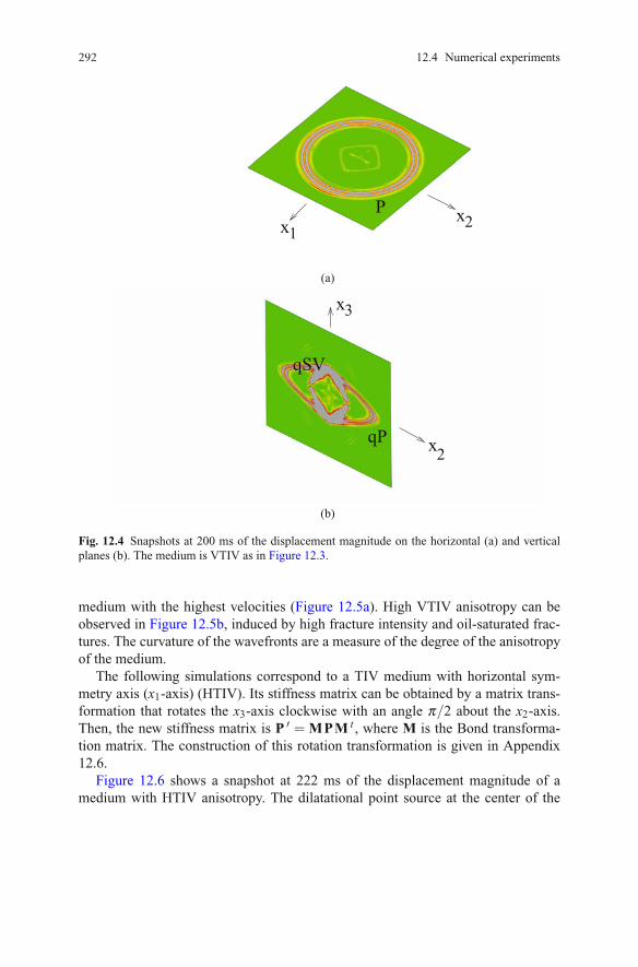
292qP
Px
x21
(a)
qP
qSV
x
x
2
3
(b)
Fig. 12.4 Snapshots at 200 ms of the displacement magnitude on the horizontal (a) and verticalplanes (b). The medium is VTIV as in Figure 12.3.
medium with the highest velocities (Figure 12.5a). High VTIV anisotropy can beobserved in Figure 12.5b, induced by high fracture intensity and oil-saturated frac-tures. The curvature of the wavefronts are a measure of the degree of the anisotropyof the medium.
The following simulations correspond to a TIV medium with horizontal sym-metry axis (x1-axis) (HTIV). Its stiffness matrix can be obtained by a matrix trans-formation that rotates the x3-axis clockwise with an angle π/2 about the x2-axis.Then, the new stiffness matrix is P ′ = MPM t , where M is the Bond transforma-tion matrix. The construction of this rotation transformation is given in Appendix12.6.
Figure 12.6 shows a snapshot at 222 ms of the displacement magnitude of amedium with HTIV anisotropy. The dilatational point source at the center of the
12.4 Numerical experiments

12 The macro-scale. Wave propagation in transversely isotropic media 293
x
x
3
2
qSV qP
P
(a)x
x2
3
qPqSV
P
(b)
Fig. 12.5 Snapshots at 200 ms of the magnitude of displacement on two orthogonal planes. VTIVanisotropy of very low-order for low fracture intensity and gas saturated fractures (a) and high-order VTIV anisotropy for high fracture intensity and oil saturated fractures (b). The source is adilatational point perturbation at the center of the domain.
domain generate a qP-wave and a slow (qS2) shear-wave in the (x1,x3) and (x1,x2)planes. In this example, the (x2,x3) plane is oriented in the direction of the verticalfractures and behaves isotropically.
In order to highlight the S-waves propagation split, we consider a S-wave sourceas a strain ε12 = 1 defined by the distribution ε12δx1s ,x2s ,x3s
located at the center ofthe horizontal plane (x1,x2) , i.e.(∂δx1s ,x2s ,x3s
∂x2,
∂δx1s ,x2s ,x3s
∂x1)
). (12.9)
Figure 12.7 illustrates fast and slow S-waves corresponding to directions paralleland normal to the fractures, respectively. Consequently, 9-c multicomponent seismic

294
P
qP
qP
qSV
xx
x3
21
Fig. 12.6 Snapshot at 222 ms of the displacement magnitude on three orthogonal planes. Themedium is HTI with high fracture intensity and gas saturated fractures. The source is a dilatationalpoint perturbation.
can be simulated using these techniques and shear sources similar to the one in(12.9).
12.5 2-D seismic imaging of an anisotropic layer
The model consists of an isotropic cubic background, Ω , of 1600 m side lengthcontaining an horizontal anisotropic layer of 400 m thickness. Anisotropy is inducedby the presence of either vertical or horizontal aligned fractures (HTIV or VTIVmedium).
The stiffnesses components of the anisotropic layer were determined using thetime-harmonic experiments for the cases of fully brine saturated or 10 % patchybrine-gas saturation in background and fractures. Fractures are modeled as thin lay-ers of aperture 1 cm and the fracture intensity is 6 fractures per meter.
The isotropic background has P- and S-wave velocities at 50 Hz equal to 2633m/s and 1270 m/s, respectively.
For the HTIV-case, qP- and qSV-wave velocities at 50 Hz are equal to 3808 m/sand 1686 m/s, respectively, while for the VTIV-case qP- and qSV-wave velocities at50 Hz are equal to 3008 m/s and 1686 m/s, respectively.
The computational mesh consists of cubic cells of side length 4 m, and the sourceis a line dilatational perturbation in the x2-direction of central frequency 50 Hz, lo-cated at (x1=800 m, x3=6 m). A line of receivers determining the vertical plane islocated near the surface (x3=0). Figure 12.8 shows a vertical section of the modelwith the location of source indicated in the figure by a yellow triangle and the re-ceivers displayed as black squares.
12
.
5 2-D seismic imaging of an anisotropic layer

12 The macro-scale. Wave propagation in transversely isotropic media 295
xx
x
1
2
3
P
S1
qP
S2
(a)
S1S2
qPx x
x
1 2
3
(b)
Traces in Figure 12.9 show reflections from the top and bottom of the HTIV andVTIV layers for the case of brine-saturated background and with fractures. It canbe seen that the reflection from the top of the VTIV layer has lower amplitude thanthe corresponding one of the HTIV layer due to the lower reflectivity of the VTIVlayer. The reflection from the bottom of the VTIV layer is delayed and attenuated ascompare with the HTIV arrival due to lower velocity and high attenuation sufferedby qP-waves travelling within the VTIV layer, in accordance with Figure 12.2.
Figure 12.10 show traces displaying reflections from the top and bottom of theHTIV layer for the cases of brine and patchy brine-gas saturated background andfractures. The arrival times correspond to the speed of the media with a slight delayand greater attenuation rates in the presence of the gas patches.
The synthetic seismograms in Figure 12.11 correspond the HTIV and VTIV lay-ers with brine saturated background and fractures. The seismograms show the ar-
Figures 12.9 and 12.10 display traces measured at a receiver located inmediately below the source location.
Fig. 12.7on the three orthogonal planes at 200 ms (a) and 300 ms (b). The medium is HTIV with highfracture intensity and gas-filled fractures. The perturbations are generated by a shear source at thecenter of the (x1,x2) plane.
Snapshot of the displacement magnitude for fast and slow (S1 and S2) split S-waves

296
(a) (b)
Fig. 12.8 2-D model with source and line of receivers. Isotropic background and the embeddedhorizontal anisotropic layer. HTIV layer (a) and VTIV layer (b).
0 200 400 600Time (ms)
-8e-06
-6e-06
-4e-06
-2e-06
0
2e-06
4e-06
6e-06
8e-06
z-co
mpo
nent
of p
artic
le v
eloc
ity (m
)
Reflection from bottom of HTI layer
Reflection from top of
HTIVTI
Reflection from bottom of VTI layer
anisotropic layer
3x
Fig. 12.9 Synthetic traces. HTIV and VTIV brine saturated fractures.
rivals of P and S waves reflected at the top of the HTIV (Figure 12.11a) and VTIV(Figure 12.11b) layers, as well as later arrivals corresponding to conversions fromincident P to qP and qSV waves at the top and bottom of the layers. In particular, itis clearly seen the late P-qP-P arrival of the VTIV case as compared with the corre-sponding one in the HTIV case. The qP-velocities in the HTIV and VTIV layers areabout 3800 m/s and 3000m/s, respectively.
Finally, seismograms for the HTIV layer with brine and 10 % gas saturated back-ground and fractures are shown in Figure 12.12. They display the arrivals of P and
12 5 2-D seismic imaging of an anisotropic layer

12 The macro-scale. Wave propagation in transversely isotropic media 297
0 200 400 600 800Time (ms)
-8e-06
-6e-06
-4e-06
-2e-06
0
2e-06
4e-06
6e-06
8e-06
z-co
mpo
nent
of p
artic
le v
eloc
ity (m
)
Brine saturated fracturesPatchy brine-CO2 saturated fractures
Reflections from top
of HTI layer
Reflections from bottom of HTI layer
P-qP-qP-qP-qP-P multiple reflection
3x
Fig. 12.10 Synthetic traces. HTIV medium with brine and patchy brine-gas saturated fractures.
0
0.2
0.4
0.6
0.8
Tim
e (s
)
50 100 150Geophone
P−qP−qSV−S
P−qP−qP−qP−qP−P
P−qP−qP−SP−qP−P
P−S
P−P
0
0.2
0.4
0.6
0.8
Tim
e (s
)
50 100 150Geophone
P−qP−qSV−SP−qP−qP−qP−qP−P
P−qP−P
P−qP−S
P−P
(a) (b)
Fig. 12.11 Synthetic seismograms. HTIV (a) and VTIV (b) brine saturated fractures.
S waves reflected at the top of the HTIV layer, and later arrivals corresponding toconversions from incident P to qP and qSV waves at the top and bottom of the layer.In particular, the P-qP-qP-qP-qP-P arrival in the brine-saturated case is not seen inthe patchy brine-gas case due to the strong attenuation of qP waves when gas ispresent (Qp≈ 10 at normal incidence). Instead qSV-waves are less attenuated whengas is present and the P-qP-qSV-S-arrival is still observed.

298
0
0.2
0.4
0.6
0.8
Tim
e (s
)
50 100 150Geophone
P−qP−qSV−S
P−qP−qP−qP−qP−P
P−qP−qP−SP−qP−P
P−S
P−P
0
0.2
0.4
0.6
0.8
Tim
e (s
)
50 100 150Geophone
P−qP−qSV−S
P−qP−qP−S
P−qP−P
P−S
P−P
(a) (b)
Fig. 12.12 Synthetic seismograms. HTIV medium with brine (a) and 10 % gas (b) saturated frac-tures.
12.6 Appendix 1. Rotation transformation in R3
Elemental rotation about one of the axes of a coordinate system can be expressed by
A=
⎛⎝ a11 a12 a13
a21 a22 a23
a31 a32 a33
⎞⎠and the Bond transformation matrix is
M=
⎛⎜⎜⎜⎜⎜⎜⎝a2
11 a212 a2
13 2 a12 a13 2 a13 a11 2 a11 a12
a221 a2
22 a223 2 a22 a23 2 a23 a21 2 a21 a22
a231 a2
32 a233 2 a32 a33 2 a33 a31 2 a31 a32
a21 a31 a22 a32 a23 a33 a22 a33 +a23 a32 a21 a33 +a23 a31 a22 a31 +a21 a32
a31 a11 a32 a12 a33 a13 a12 a33 +a13 a32 a13 a31 +a11 a33 a11 a32 +a12 a31
a11 a21 a12 a22 a13 a23 a12 a23 +a13 a22 a13 a21 +a11 a23 a11 a22 +a12 a21
⎞⎟⎟⎟⎟⎟⎟⎠.
Then, the rotation applied to the stiffness matrix of the TI medium with verticalsymmetry axis is
A=
⎛⎝ cosθ 0 −sinθ0 1 0
sinθ 0 cosθ
⎞⎠=
⎛⎝0 0 −10 1 01 0 0
⎞⎠
12.6 Appendix 1. Rotation transformation in R3
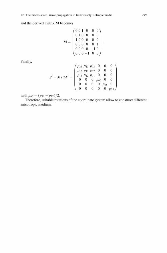
12 The macro-scale. Wave propagation in transversely isotropic media 299
and the derived matrix M becomes
M=
⎛⎜⎜⎜⎜⎜⎜⎝0 0 1 0 0 00 1 0 0 0 01 0 0 0 0 00 0 0 0 0 10 0 0 0 −1 00 0 0 −1 0 0
⎞⎟⎟⎟⎟⎟⎟⎠ .
Finally,
P′ =MPM t =
⎛⎜⎜⎜⎜⎜⎜⎝p33 p13 p13 0 0 0p13 p11 p12 0 0 0p13 p12 p11 0 0 00 0 0 p66 0 00 0 0 0 p55 00 0 0 0 0 p55
⎞⎟⎟⎟⎟⎟⎟⎠with p66 = (p11 − p12)/2.
Therefore, suitable rotations of the coordinate system allow to construct differentanisotropic medium.

Glossary
us : displacement vector of the solid
u f : displacement vector of the fluid
uθ ,θ = o,w,g : displacement vectors of the θ -fluid
ω : angular frequency
Km : dry matrix bulk modulus
μm : dry matrix shear modulus
Ks : bulk modulus of the solid grains
μs : shear modulus of the solid grains
κ : permeability
φ : porosity
Krn(Sn),Krw(Sn),Krnw(Sn) : relative permeabilities for two-phase fluids
Krθ (Sθ ),θ = o,w,g : relative permeabilities for three-phase fluids
τi j : stress tensor components of the bulk material
σi j : stress tensor components of the solid matrix
εi j : strain tensor at the mesoscale
ei j : strain tensor at the macroscale
p f : fluid pressure
pθ ,θ = o,w,g : pressure of the θ -fluid
Pca(Sn) : capillary pressure function for two-phase fluids
Pcow(So),Pcgo(Sg) : capillary pressure functions for three-phase fluids
© Springer International Publishing AG 2016
in Geosystems Mathematics and Computing, DOI 10.1007/978-3-319-48457-0
301J.E. Santos, P.M. Gauzellino, Numerical Simulation in Applied Geophysics, Lecture Notes

302 Glossary
Sn : saturation of the nonwetting phase
Sw : saturation of the wetting phase
Sθ ,θ = o,w,g : saturation of the θ -fluid
λ : Lame parameter of the open system
λu : Lame parameter of the closed system
Ku : Bulk modulus of the undrained material
W : strain energy density
Td : kinetic energy density
Vd : potential energy density
Dd : dissipation energy density
Ku : Gassmann bulk modulus of the undrained system
ζ : Change in fluid content
η : fluid viscosity
ηθ ,θ = o,w,g : viscosity of the θ -fluid
ρ f : fluid density
ρθ : density of the θ -fluid
ρs : density of the solid grains
ρ : bulk density
gθ ,bθ ,θ = o,w,g : mass and viscous couplig coefficients for three-phase fluids
glt ,blt ,(l, t) == (o,w),(o,g),(w,g) : cross mass and viscous couplig coefficients
gn,gw,gnw,bn,bw,bnw : mass and viscous couplig coefficients for two-phase fluids
ηN ,ηT : normal and tangential fracture compliances
for three-phase fluids
pIJ , I,J1 6: stiffness coefficients≤ ≤

References
[Adams, 1975] Adams, R.A.: Sobolev Spaces. Academic Press (1975)[Arntsen and Carcione, 2001] Arntsen, B., Carcione, J. M.: Numerical simulation of the Biot slow
wave in water-saturated Nivelsteiner sandstone. Geophysics, 66, 890–896 (2001)[Arts et al., 2008] Arts, R., Chadwick, A., Eiken, O., Thibeau, S., Nooner, S.: Ten years of ex-
perience of monitoring CO2 injection in the Utsira sand at Sleipner, offshore Norway. FirstBreak, 26, 65–72 (2008)
[Auriault et al., 1985] Auriault, J.L., Borne, L., Chambon, R.: Dynamics of porous saturated me-dia, checking of the generalized law of Darcy. J. Acoust. Soc. Am., 77, 1641–1650 (1985)
[Aziz and Settari, 1985] Aziz, K., Settari, A.: Petroleum Reservoir Simulation. Elsevier AppliedScience Publishers, Great Britain (1985)
[Baker, 1988] Baker, I.E.: Three-phase relative permeability correlations. In: Proceedings of Soci-ety of Petroleum Engineers Enhanced Oil Recovery Symposium, paper SPE-17369-MS, pp.539–554. Tulsa, Oklahoma, USA (1988)
[Backus, 1962] Backus, G.E.: Long-wave elastic anisotropy produced by horizontal layering. J.Geophys. Res., 67, 4427–4440 (1962)
[Bear, 1972] Bear, J.: Dynamics of fluids in porous media. Dover Publications, New York (1972)[Becker et al., 1981] Becker, E.B., Carey, G.F., Oden, T.: Finite elements. An introduction. Vol-
ume 1. Prentice Hall, Englewood Cliffs, New Jersey (1981)[Bensoussan, et al., 1978] Bensoussan, A., Lions, J.L., Papanicolaou, G.C.: Asymptotic analysis
for periodic structures. In: Studies in Mathematics and its Applications, 5, North-Holland(1978)
[Ben-Menahem and Sing, 1981] Ben-Menahem, A.B. and Singh, S.J.: Seismic Waves andSources. Springer-Verlag (1981)
[Berryman, 1981] Berryman, J.: Elastic wave propagation in fluid-saturated porous solids. J.Acoust. Soc. Am., 69, 416–424 (1981)
[Berryman et al., 1988] Berryman, J., Thigpen, L., Chin, R.: Bulk elastic wave propagation inpartially saturated porous solids. J. Acoust. Soc. Am., 84, 360–373 (1988)
[Biot, 1956a] Biot, M.A.: Theory of propagation of elastic waves in a fluid-saturated porous solid.I. Low-frequency range. J. Acoust. Soc. Am., 28, 168–178 (1956)
[Biot, 1956b] Biot, M.A.: Theory of propagation of elastic waves in a fluid-saturated porous solid.II. Higher frequency range. J. Acoust. Soc. Am., 28, 179–191 (1956)
[Biot, 1962] Biot, M.A.: Mechanics of deformation and acoustic propagation in porous media. J.Appl. Phys., 33, 1482–1498 (1962)
[Biot and Willis, 1957] Biot, M.A., Willis, D.G.: The elastic coefficients of the theory of consoli-dation. J. Appl. Mech., 24, 594–601 (1957)
[Bourbie et al., 1987] Bourbie,T., Coussy, O., Zinszner, B.: Acoustics of porous media. Technip,Paris (1987)
© Springer International Publishing AG 2016
in Geosystems Mathematics and Computing, DOI 10.1007/978-3-319-48457-0
303J.E. Santos, P.M. Gauzellino, Numerical Simulation in Applied Geophysics, Lecture Notes

304 References
[Brown and Korriga, 1975] Brown, R.J.S., Korringa, J.: On the dependence of the elastic proper-ties of a porous rock on the compressibility of a pore fluid. Geophysics, 40, 608–616 (1975)
[Burridge and Keller, 1981] Burridge, R., Keller, J.B.: Poroelasticity equations derived from mi-crostructure. J. Acoust. Soc. Am., 70, 1140–1146 (1981)
[Cadoret et al., 1995] Cadoret, T., Marion, D., Zinszner, B.: Influence of frequency and fluid dis-tribution on elastic wave velocities in partially saturated lime- stones. J. Geophys. Res., 100,9789–9803 (1995)
[Carcione et al., 1991] Carcione, J.M., Kosloff, D., Behle, A.: Long wave anisotropy in stratifiedmedia: a numerical test. Geophysics, 56, 245–254 (1991)
[Carcione, 1992] Carcione, J.M.: Anisotropic Q and velocity dispersion of finely layered media.Geophys. Prosp., 40, 761–783 (1992)
[Carcione et al., 1994] Carcione, J.M., Boehm G., Marchetti, A.: Simulation of a CMP seismicsection. J. Seismic Expl., 3, 381–396 (1994)
[Carcione, 1996] Carcione, J.M.: Plane-layered models for the analysis of wave propagation inreservoir environments. Geophys. Prosp., 44, 3–26 (1996)
[Carcione and Seriani, 1998] Carcione J.M., Seriani, G.: Seismic velocities in permafrost. Geo-phys. Prosp., 46, 441–454 (1998)
[Carcione et al., 2000] Carcione, J.M., Gurevich B., Cavallini F.: A generalized Biot-Gassmannmodel for the acoustic properties of shaley sandstones. Geophys. Prosp., 48, 539–557 (2000)
[Carcione and Tinivella, 2000a] Carcione, J.M., Tinivella U.: Bottom-simulating reflectors: Seis-mic velocities and AVO effects. Geophysics, 65, 54–67 (2000)
[Carcione et al., 2003] Carcione, J.M., Helle, H.B., Pham, N.H.: Whites model for wave prop-agation in partially saturated rocks: Comparison with po- roelastic numerical experiments.Geophysics, 68, 1389–1398 (2003)
[Carcione et al., 2003] Carcione, J.M., Helbig, K., Helle, H.B.: Effects of pressure and saturatingfluid on wave velocity and attenuation of anisotropic rocks. Int. J. Rock Mech. Min. Sci., 40,389–403 (2003)
[Carcione et al., 2004] Carcione, J.M., Cavallini, F., Santos, J.E., Ravazzoli, C.L., Gauzellino,P.M.: Wave propagation in partially-saturated porous media: Simulation of a second slowwave. Wave Motion, 39, 227–240 (2004)
[Carcione and Picotti, 2006] Carcione, J.M., Picotti, S.: P-wave seismic attenuation by slow-wavediffusion, Effects of inhomogeneous rock properties. Geophysics, 71, 1–8 (2006)
[Carcione et al., 2012] Picotti, S., Carcione, J.M., Gei, D., Rossi, G., Santos, J.E.: Seismic model-ing to monitor CO2 geological storage - 1 the Atzbach-Schwanenstadt gas field. J. Geophys.Res., 117, 1–18 (2012)
[Carcione et al., 2012] Carcione, J.M., Santos, J.E., Picotti, S.: Fracture induced anisotropic at-tenuation. Rock Mech. Rock Eng., 45, 929–942 (2012)
[Carcione, 2014] Carcione, J.M.: Wave fields in real media: wave propagation in anisotropic,anelastic, porous and electromagnetic media. 3rd ed., Elsevier (2014)
[Carcione et al., 2013] Carcione, J.M., Gurevich, B., Santos, J.E., Picotti, S.: Angular and fre-quency dependent wave velocity and attenuation in fractured porous media. Pure Appl. Geo-phys., 170, 1673–1683 (2013)
[Chadwick et al., 2005] Chadwick, R.A., Arts, R., Eiken, O.: 4D seismic quantification of a grow-ing CO2 plume at Sleipner, North Sea. In: Dore, A.G. and Vincent, B. (eds.) Petroleum Geol-ogy: North West Europe and Global Perspectives - Proc. 6th Petroleum Geology Conference,1385–1399 (2005)
[Chadwick et al., 2009] Chadwick, R.A., Noy, D., Arts, R., Eiken, O.: Latest time-lapse seismicdata from Sleipner yield new insights into CO2 plume development. Energy Procedia, 1,2103–2110 (2009)
[Chadwick et al., 2010] Chadwick, R.A., Williams, G., Delepine, N., Clochard, V., Labat, V., Stur-ton, S., Buddensiek, M., Dillen, M., Nickel, M., Lima, A., Arts, R., Neele, F., Rossi, G.: Quan-titative analysis of time-lapse seismic monitoring data at the Sleipner CO2 storage operation.The Leading Edge, 29, 170–77 (2010)
[Ciarlet, 1976] Ciarlet, P.: The finite elements method for elliptic problems. North Holland,Amsterdam-New York-Oxford (1976)

References 305
[Collins, 1961] Collins, R.E.: Flow of fluids through porous materials. Reinhold Publishing Co.,New York (1961)
[Chavent and Jaffre, 1986] Chavent, G. and Jaffre, J.: Mathematical models and finite elementsfor reservoir simulation. Elsevier Science Publishers B.V., North Holland (1986)
[Corapcioglu, 1996] Corapcioglu, M.Y.: Advances in porous media, Volume 3. Elsevier Science(1996)
[Deptuck et al., 1985] Deptuck, D., Harrison, J.P., Zawadzki, P.: Measurement of elasticity andconductivity in a three-dimensional percolation system. Phys. Rev. Lett., 54, 913–916 (1985)
[Douglas Jr. et al., 1993] Douglas, J. Jr., Hensley, J.L., Paes Leme, P.J.: A study of the effect of in-homogeneities on immiscible flow in naturally fractured reservoirs. Int. Series Numer. Math.(Birkhauser Verlag Basel), 114, 59–74 (1993)
[Douglas Jr. et al., 1993a] Douglas, J. Jr., Santos, J.E., Sheen, D., Bennethum, L.S.: Frequencydomain treatment of one-dimensional scalar waves. Math. Models Meth. Appl. Sci., 3, 171–194 (1993)
[Douglas Jr. et al., 1994] Douglas, J. Jr., Santos, J.E., Sheen, D.: Approximation of scalar wavesin the space-frequency domain, Math. Models Meth. Appl. Sci., 4, 509–531 (1994)
[Douglas Jr. et al., 1997] , Douglas, J. Jr, Furtado, F., Pereira, F.: The statistical behavior of insta-bilities in immiscible displacement subject to fractal geology. In: Burgeaut, A., Carasso, C.,Luckhaus, S., Mikelic, A. (eds.). Mathematical Modeling of Flow Through Porous Media,pp. 115–137, World Scientific, Singapore (1997)
[Douglas Jr. et al., 1999] Douglas, J. Jr., Santos, J.E., Sheen, D., Ye, X.: Nonconforming Galerkinmethods based on quadrilateral elements for second order elliptic problems. Math. Modell.Numer. Analysis, 33, 747–770 (1999)
[Douglas Jr. et al., 2001] Douglas, J. Jr., Santos, J.E., Sheen, D.: Nonconforming Galerkin meth-ods for the Hemholtz equation. Numer. Meth. Part. Diff. Equat., 17, 475–494 (2001)
[Dutta and Ode, 1979] Dutta, N.C., Ode, H.: Attenuation and dispersion of compressional wavesin fluid-filled porous rocks with partial gas saturation (White model) - Part I: Biot theory.Geophysics, 44, 1777–1788 (1979)
[Dutta and Ode, 1983] Dutta, N.C. and Ode, H.: Seismic reflections from a gas-water contact.Geophysics, 48, 148–162 (1983)
[Dvorkin et al., 1995] Dvorkin, J., Mavko, G., Nur, A.: Squirt flow in fully saturated rocks. Geo-physics, 60, 97–107 (1995)
[Fabrizio and Morro, 1992] Fabrizio, M., Morro, A.: Mathematical problems in linear viscoelas-ticity. SIAM Studies in Applied Mathematics, 12, Philadelphia (1992)
[Fanchi, 1997] Fanchi, J.R.: Principles of Applied Reservoir Simulation. Gulf Professional Pub-lishing Co., Houston, Texas (1997)
[Ferry, 1970] Ferry, J.D.: Viscoelastic properties of polymers. John Wiley (1970)[Frankel and Clayton, 1986] Frankel, A., Clayton, R.W.: Finite difference simulation of seismic
wave scattering: implications for the propagation of short period seismic waves in the crustand models of crustal heterogeneity. J. Geophys. Res., 91, 6465–6489 (1986)
[Fung, 1965] Fung, Y.C.: Foundations of solid mechanics. Prentice Hall, Englewood Cliffs, NewJersey (1965)
[Gassmann, 1951] Gassmann, F.: Uber die Elastizitat poroser Mediem. Vierteljahrsschr Natur-forsch. Ges. Zurich, 96, 1–23 (1951)
[Gauzellino et al., 2001] Gauzellino, P.M., Santos, J.E., Sheen D.: Frequency domain wave prop-agation modelling in exploration seismology. J. Comp. Acoust., 12, 941–955 (2001)
[Gauzellino et al., 2014] Gauzellino, P.M., Santos, J.E., Carcione, J.M., Picotti, S.: A rheologicalequation for anisotropic-anelastic media and simulation of field seismograms. Wave Motion,51, 743–757 (2014)
[Gelinsky and Shapiro, 1997] Gelinsky, S., Shapiro, S.A.: Poroelastic Backus-averaging foranisotropic, layered fluid and gas saturated sediments. Geophysics, 62, 1867–1878 (1997)
[Gurevich and Lopatnikov, 1995] Gurevich, B., Lopatnikov, S.L.: Velocity and attenuation ofelastic waves in finely layered porous rocks. Geophys. J. Int., 121, 933–947 (1995)
[Gurevich et al., 1997] Gurevich, B., Zyrianov, V.B., Lopatnikov, S.L.: Seismic attenuation in fin-ley layered porous rocks: Effects of fluid flow and scattering. Geophysics, 62, 319–324 (1997)

306 References
[Gurevich, 2003] Gurevich, B.: Elastic properties of saturated porous rocks with aligned fractures.J. Appl. Geophys., 54, 203–218 (2003)
[Gurevich et al., 2009] Gurevich, B., Brajanovski, M., Galvin, R.J., Muller, T.M., Toms-Stewart,J.: P-wave dispersion and attenuation in fractured and porous reservoirs-poroelasticity ap-proach. Geophys. Prosp., 57, 225–237 (2009)
[Ha et al., 2002] Ha, T., Santos, J.E., Sheen, D.: Non-conforming finite element methods for thesimulation of waves in viscoelastic solids. Comp. Meth. Appl. Mech. Eng., 191, 5647–5670(2002)
[Han et al., 1986] Han, D.H., Nur, A., Morgan, D.: Effects of porosity and clay content on wavevelocities in sandstones. Geophysics, 51, 2093–2107 (1986)
[Hashin and Shtrikman, 1963] Hashin, Z., Shtrikman, S.: A variational approach to the elasticbehavior of multiphase minerals. J. Mech. and Phys. Solids, 11, 127–140 (1963)
[Hassanzadeh et al., 2008] Hassanzadeh, H., Pooladi-Darvish, M., Elsharkawy, A., Keith, D.,Leonenko, Y.: Predicting PVT data for CO2-brine mixtures for black-oil simulation of CO2geological storage. Int. J. Greenhouse Gas Control, 2, 65–77 (2008)
[Helle et al., 2003] Helle, H.B., Pham, N.M., Carcione, J.M.: Velocity and attenuation in partiallysaturated rocks: poroelastic numerical experiments. Geophys. Prosp., 51, 551–566 (2003)
[Hill, 1964] Hill, R.: Theory of mechanical properties of fiber-strengthened materials. J. Mech.Phys. Solids, 11, 357–372 (1964)
[Hovem and Ingram, 1979] Hovem, J.M., Ingram, G.D.: Viscous attenuation of sound in saturatedsand. J. Acoust. Soc. Am., 66, 1807–1812 (1979)
[Ihlenburg and Babuska, 1997] Ihlenburg, F., Babushka, I.: Solution of Helmholtz problems byknowledge-based FEM. Comp. Assisted Mech. Eng. Sci., 4, 397–415 (1997)
[Johnson et al., 1987] Johnson D.L., Koplik J., Dashen R.: Theory of dynamic permeability andtortuosity in fluid-saturated porous media. J. Fluid Mech., 176, 379–402 (1987)
[Johnson, 2001] Johnson, D.L.: Theory of frequency dependent acoustics in patchy-saturatedporous media. J. Acoust. Soc. Am., 110, 682–694 (2001)
[Jones, 1986] Jones, T.D.: Pore-fluids and frequency dependent wave propagation rocks. Geo-physics, 51, 1939–1953 (1986)
[Keller, 1989] Keller, J.D.: Acoustic wave propagation in composite fluid-saturated media. Geo-physics, 54, 1554–1563 (1989)
[Kelder and Smeulders, 1997] Kelder, O., Smeulders, D.: Observation of the Biot slow wave inwater-saturated Nivelsteiner sandstone. Geophysics, 62, 1794–1796 (1997)
[Dahlberg et al., 1988] Dahlberg, B.E.J., Kenig, C.E., Verchota, G.C.: Boundary value problemsfor the systems of elastostatics in Lipschitz domains. Duke Math. J., 57, 795–818 (1988)
[Kim, 1995] Kim, S.: Parallel multidomain iterative algorithms for the Helmholtz wave equation.Appl. Numer. Math., 17, 411–429 (1995)
[Kolmogorov and Fomin, 1970] Kolmogorov, A.N., Fomin, S.V.: Introductory Real Analysis.Dover Publications, Inc., New York (1970)
[Kolsky, 1963] Kolsky, H.: Stress Waves in Solids. Dover publications, New York (1963)[Krief et al., 1990] Krief M., Garat J., Stellingwerff J., Ventre J.: A petrophysical interpretation
using the velocities of P and S waves (full waveform sonic). The Log Analyst, 31, 355–369(1990)
[Krzikalla and Muller, 2011] Krzikalla, F., Muller, T. M.: Anisotropic P-SV-wave dispersion andattenuation due to inter-layer flow in thinly layered porous rocks. Geophysics, 76, WA135–WA145 (2011)
[Kuster and Toksoz, 1974] Kuster, G.T., Toksoz, M.N.: Velocity and attenuation of seismic wavesin two-phase media: Part 1. Theoretical formulations. Geophysics, 39, 587–606 (1974)
[Leclaire et al., 1994] Leclaire, P., Cohen-Tenoudji, F., Aguirre Puente, J.: Extension of Biots the-ory to wave propagation in frozen porous media. J. Acoust. Soc. Am., 96, 3753–3767 (1994)
[Leclaire et al., 1985] Leclaire, P., Cohen-Tenoudji, F., Aguirre Puente, J.: Observation of twolongitudinal and two transverse waves in a frozen porous medium. J. Acoust. Soc. Am., 97,2052–2055 (1995)
[Levy, 1979] Levy, T.: Propagation of waves in a fluid-saturated porous elastic solid. Int. J. Eng.Sci., 17, 1005–1014 (1979)
References 307
[Liu et al., 1976] Liu, H.P., Anderson, D.L., Kanamori, H.: Velocity dispersion due to anelasticity;implications for seismology and mantle composition. Geophys. J. R. Astr. Soc., 47, 41–58(1976)
[Lo et al., 2005] Lo, W.C., Sposito, G., Majer, E.: Wave propagation through elastic porous mediacontaining two immiscible fluids. Water Resour. Res., 41, W02025, 1–20 (2005)
[Loeve, 1944] Loeve, A.E.: A Treatise on the Mathematical Theory of Elasticity. 4th ed., Dover,New York (1944)
[Lovera and Santos, 1988] Lovera O.M., Santos J.E.: Numerical methods for a model for wavepropagation in composite anisotropic media. Math. Modell. Numer. Analysis, 22, 159–176(1988)
[Lumley and Panofsky, 1964] Lumley, J., Panofsky, H: The structure of atmospheric turbulence.Interscience Publishers, New York (1964)
[Masson and Pride, 2007] Masson, Y.J., Pride, S.R.: Poroelastic finite difference modelling ofseismic attenuation and dispersion due to mesoscopic-scale heterogeneity. J. Geophys. Res.,112, B03204 (2007)
[Mavko et al., 1998] Mavko, G., Mukerji, T., Dvorkin, J.: The Rock Physics Handbook. Cam-bridge University Press (1998)
[McCoy, 1983] McCoy, R.L.: Microcumputers programs for Petroleum Engineers, Volume 1,Gulf Publishing Co. Houston, Texas (1983)
[Mochizuki, 1982] Mochizuki, S.: Attenuation in partially saturated rocks. J. Geophys. Res., 87,8598–8604 (1982)
[Morack and Rogers, 1981] Morack, J.L., Rogers, J.C.: Seismic evidence of shallow permafrostbeneath the islands in the Beafort Sea. Artic, 3, 166–174 (1981)
[Muller and Gurevich, 2005] Muller, T., Gurevich, B.: Wave-induced fluid flow in random porousmedia: Attenuation and dispersion of elastic waves. J. Acoust. Soc. Am., 117, 2732–2741(2005)
[Muller and Toms, 2007] Muller, T., Toms, J.: Velocity-saturation relation for rocks with fractaldistribution of the pore fluids. In: 77th Ann. Internat. Mtg., Soc. Expl. Geophys., San Antonio,USA, Expanded Abstracts, 1624–1628 (2007)
[Nakagawa and Schoenberg, 2007] Nakagawa, S., Schoenberg, M.A.: Poroelastic modeling ofseismic boundary conditions across a fracture. J. Acoust. Soc. Ame., 122, 831–847 (2007)
[Nedelec, 1980] Nedelec, J.C.: Mixed finite elements in R3. Numerische Mathematik, 35, 315–341 (1980)
[Norris, 1993] Norris, A.N.: Low-frequency dispersion and attenuation in partially saturatedrocks. J. Acoust. Soc. Am., 94, 359–370 (1993)
[O’Connell and Budiansky, 1974] OConnell, R., Budiansky, B.: Seismic velocities in dry and sat-urated cracked solids. J. Geophys. Res., 79, 5412–5426 (1974)
[Picotti et al., 2010] Picotti, S., Carcione, J.M., Santos, J.E., Gei, D.: Q-anisotropy in finely-layered media. Geophys. Res. Lett., 37, L06302 (2010)
[Picotti et al., 2012] Picotti, S, Carcione, J.M., Gei, D., Rossi, G., Santos, J.E.: Seismic modelingto monitoring CO2 geological storage. The Atzbach-Schwanenstadt gas field. J. Geophys.Res., 117, B06103 (2012)
[Peaceman, 1977] Peaceman, D.W.: Fundamentals of numerical reservoir simulation. Elsevier(1977)
[Peng and Robinson, 1976] Peng, D.Y., Robinson, K.I.: A new two-constant equation of state, Ind.Eng. Chem. Fundam., 15, 59–64 (1976)
[Pride and Berryman, 2003] Pride, S.R., Berryman, J.G.: Linear dynamics of double-porosity anddual-permeability materials. I. governing equations and acoustic attenuation. Phys. Rev. E,68, 036603 (2003)
[Pride et al., 2004] Pride, S.R., Berryman, J.G., Harris, J.M.: Seismic attenuation due to wave-induced flow. J. Geophys. Res., 109, B01201 (2004)
[Pyrak-Nolte et al., 1990] Pyrak-Nolte, L.J., Myer, L.R., Cook, N.G.: Anisotropy in seismic ve-locities and amplitudes from multiple parallel fractures. J. Geophys. Res., 95, 11345–11358(1990)

308 References
[Rasolofosaon, 1991] Rasolofosaon, P.: Plane acoustic waves in linear viscoelastic porous media:energy, particle displacement and physical interpretation. J. Acoust. Soc. Am., 89, 1532–1550(1991)
[Ravazzoli and Santos, 1995] Ravazzoli, C.L., Santos, J.E.: Consistency analysis for a model forwave propagation in anelastic media. Latin Am. Appl. Res., 25, 141–152 (1995)
[Ravazzoli et al., 2003] Ravazzoli, C.L., Santos, J.E., Carcione, J.M.: Acoustic and mechanicalresponse of reservoir rocks under varaible saturation and effective pressure. J. Acoust. Soc.Am., 113, 1801–1811 (2003)
[Raviart and Thomas, 1977] Raviart, P.A., Thomas, J.M.: A mixed finite element method for sec-ond order elliptic problems. In: Galligani, I., Magenes, E. (eds.). Mathematical Aspects ofthe Finite Element Method, Element Method, Lecture Notes in Mathematics, 606, 292–315(1977)
[Rubino et al., 2007] Rubino, J.G., Santos, J.E., Picotti, S., Carcione, J.M.: Simulation of upscal-ing effects due to wave-induced fluid flow in Biot media using the finite-element method. J.Appl. Geophys., 62, 193–203 (2007)
[Rubino et al., 2008] Rubino, J.G., Ravazzoli, C.L., Santos, J.E.: Biot-type scattering effects ingas-hydrate bearing sediments. J. Geophys. Res., Solid Earth, 113, B06102, 1–16 (2008)
[Russo and Bouton, 2007] Russo, D., Bouton, M.: Statistical analysis of spatial variability in un-saturated flow parameters. Water Resour. Res., 28, 1911–1925 (1992)
[Russo et al., 1997] Russo, D., Russo, I., Laufer, A.: On the spatial variability of parameters ofthe unsaturated hydraulic conductivity. Water Resour. Res., 33, 945–956 (1997)
[Saenger et al., 2007] Saenger E.H., Ciz, R., Kruger, O.S., Schmalholz, S.M., Gurevich, B.,Shapiro, S.A.: Finite-difference modeling of wave propagation on microscale: A snapshotof the work in progress. Geophysics 72, SM293–SM300 (2007)
[Sanchez Palencia, 1980] Sanchez-Palencia, E.: Non-homogeneous media and vibration theory.In: Lecture Notes in Physics, Springer-Verlag, New York (1980)
[Santos et al., 1988] Santos, J.E., Douglas, J. Jr., Morley, M.E., Lovera., O.M.: Finite elementmethods for a model for full waveform acoustic logging. IMA, J. Numer. Analysis, 8, 415–433 (1988)
[Santos et al., 1990a] Santos, J.E., Corbero, J.M., Douglas, J. Jr.: Static dynamic behavior of aporous solid saturated by a two-phase fluid. J. Acoust. Soc. Am., 87, 1428–1438 (1990)
[Santos et al., 1990b] Santos, J.E., Douglas, J. Jr., Corbero, J.M., Lovera, O.M.: A model for wavepropagation in a porous solid saturated by a two-phase fluid. J. Acoust. Soc. Am., 87, 1439–1448 (1990)
[Santos et al., 1992] Santos, J.E., Corbero, J.M., Ravazzoli, C.L., Hensley, J.L.: Reflection andtransmission coefficients in fluid saturated porous media. J. Acoust. Soc. Am., 91, 1911–1923(1992)
[Santos et al., 2004a] Santos, J.E., Ravazzoli, C.L., Carcione, J. M.: A model for wave propaga-tion in a porous solid saturated by a two-phase fluid. J. Acoust. Soc. Am., 87, 1439–1448(1990)
[Santos et al., 2004b] Santos, J.E., Ravazzoli, C.L., Gauzellino, P.M., Carcione, J.M., Cavallini,F.: Simulation of Waves in Poro-viscoelastic Rocks Saturated by Immiscible Fluids. Numeri-cal Evidence of a Second Slow Wave. J. Comp. Acoust., 12, 1–21 (2004)
[Santos et al., 2005a] Santos, J.E., Ravazzoli, C.L., Gauzellino, P.M., Carcione, J.M.: Numericalsimulation of ultrasonic waves in reservoir rocks with patchy saturation and fractal petrophys-ical properties. Comp. Geosciences, 9, 1–27 (2005)
[Santos et al., 2005b] Santos, J.E., Ravazzoli, C.L., Geiser, J.: On the static and dynamic behaviorof fluid saturated composite porous solids; a homogenization approach. Int. J. Solids andStructures, 43, 1224–1238 (2005)
[Santos et al., 2011] Santos, J.E., Carcione, J.M., Picotti, S.: Viscoelastic-stifness tensor ofanisotropic media from oscillatory numerical experiments. Comp. Meth. Appl. Mech. Eng.,200, 896–904 (2011)
[Santos et al., 2012] Santos, J.E., Picotti, S., Carcione, J.M.: Evaluation of the stiffness tensor ofa fractured medium with harmonic experiments. Comp. Meth. Appl. Mech. Eng., 247-248,130–145 (2012)

References 309
[Santos et al., 2014a] Santos, J.E., Martinez Corredor, R., Carcione, J.M.: Seismic velocity and Qanisotropy in fractured poroelastic media. Int. J. Rock Mech. Min. Sci., 70, 212–218 (2014)
[Santos et al., 2014b] Santos, J.E., Savioli, G.B., Macias, L., Carcione, J.M., Gei, D.: Influence ofcapillary pressure on CO2 storage and monitoring. In: Proceedings of the 84th Ann. Internat.Mtg., Soc. Expl. Geophys., Denver, USA, Expanded Abstracts, 2212–2215 (2014)
[Santos and Carcione, 2015] Santos, J.E., Carcione, J.M.: Finite-element harmonic experimentsto model fractured induced anisotropy in poroelastic media. Comp. Meth. Appl. Mech. Eng.,283, 1189–1213 (2015)
[Santos and Savioli, 2015] Santos, J.E., Savioli, G.B.: A parametric analysis of waves propagatingin a porous solid saturated by a three-phase fluid. J. Acoust. Soc. Am., 138, 3033–3042 (2015)
[Santos and Savioli, 2016] Santos, J.E., Savioli, G.B.: A model for wave propagation in a poroussolid saturated by a three-phase fluid. J. Acoust. Soc. Am., 139, 693 (2016)
[Savioli and Bidner, 2005] Savioli, G.B., Bidner, M.S.: Simulation of the oil and gas flow towarda well - a stability analysis. J. Petroleum Sci. Eng., 48, 53–69 (2005)
[Scheidegger, 1974] Scheidegger, A.E.: The physics of flow through porous media. Toronto: Uni-versity of Toronto (1974)
[Schoenberg, 1980] Schoemberg, M.: Elastic wave behavior across linear slip interfaces. J.Acoust. Soc. Am., 68, 1516–1521 (1980)
[Sheen, 1993] Sheen, D.: Finite element methods for an acoustic well-logging problem associatedwith a porous medium saturated by a two-phase immiscible fluid. Numer. Meth. Part. Diff.Equat., 9, 155–174 (1993)
[Spycher and Pruess, 2005] Spycher, N., Pruess, K.: CO2-H2O mixtures in the geological seques-tration of CO2. II. Partitioning in chloride brines at 12-100 C and up to 600 bar. Geochim.Cosmochim, Acta 69, 13, 3309–3320 (2005)
[Standing, 1977] Standing, M.B.: Volumetric and phase behavior of oil field hydrocarbon systems.Soc. Petroleum Eng. AIME, Dallas (1977)
[Stoll and Bryan, 1970] Stoll R.D., Bryan, G.M.: Wave attenuation in saturated sediments. J.Acoust. Soc. Am., 47, 1440–1447 (1970)
[Stoll, 1974] Stoll, R.D.: Acoustic waves in saturated sediments. In: Hampton L. (ed.). Physics ofSound in Marine Sediments, pp 19–39, Plenum Press (1974)
[Toms et al., 2007] Toms, J., Muller, T., Gurevich, B.: Seismic attenuation in porous rocks withrandom patchy saturation. Geophys. Prosp., 55, 671–678 (2007)
[Wenzlau et al., 2010] Wenzlau, F., Altmann, J.B., Muller, T.M.: Anisotropic dispersion and atten-uation due to wave-induced flow: quasi-static finite element modeling in poroelastic solids. J.Geophys. Res., 115, B07204 (2010)
[White et al., 1975] White, J.E., Mikhaylova, N.G., Lyakhovitskiy, F.M.: Low-frequency seismicwaves in fluid-saturated layered rocks. In: Izvestija Academy of Sciences USSR, PhysicsSolid Earth, 10, 654–659 (1975)
[White, 1975] White, J.E.: Computed seismic speeds and attenuation in rocks with partial gassaturation. Geophysics, 40, 224–232 (1975)
[Wood, 1955] Wood, A.W.: A Textbook of Sound. MacMillan Co. (1955)[Yosida, 1980] Yosida, K.: Funcional Analysis. 6th ed., Springer-Verlag, Berlin Heidelberg-New
York (1980)[Zener, 1948] Zener, C.: Elasticity of anelastic metals. The University of Chicago Press (1948)[Zimmerman et al, 1986] Zimmerman, R.W., Somerton, W.H., King, M.S.: Compressibility of
porous rocks. J. Geophys. Res., 91 NOB12, 12765–12777 (1986)[Zyserman et al., 2003] Zyserman, F.I., Gauzellino, P.M., Santos, J.E.: Dispersion analysis of a
nonconforming finite element method for the Hemholtz and elastodynamic equations. Int. J.Numer. Meth. Eng., 58, 1381-1395 (2003)
[Zyserman and Gauzellino, 2005] Zyserman, F.I., Gauzellino, P.M.: Dispersion analysis of a non-conforming finite element method for the three dimensional scalar and elastic wave equations.Finite Element in Analysis and Design, 41, 1309–1326 (2005)