..

AI

•

A Comparison of Cross-Validation

Techniques in Density Estimation!

(Comparison in Density Estimation)

by

J.S. MarronUniversity of North Carolina, Chapel Hill

AMS 1980 subject classifications: Primary 62605, Secondary 62620.

Key words and phrases: cross-validation, smoothing parameter selection,choice of nonparametric estimators, bandwidthselection.

lResearCl1 partially supported by ONR contract N00014-81-K-0373 and bySonderforschungsbereich 123 of the Deutsche Forschungsgemetnschaft.

•

•

~~~~~~

In the setting of nonparametric multivariate density estimation,

theorems are established which allow a comparison of the Kullback­

Leibler and the Least Squares cross-validation methods of smoothing

parameter selection. The family of delta sequence estimators

(including kernel, orthogonal series, histogram and histospline

estimators) is considered. These theorems also show that either

type of cross-validation can be used to compare different estimators

(eg: kernel vs. orthogonal series) .

'J

•

•

1. Introduction

Consider the problem of trying to estimate ad-dimensional

probability density function, f(x), using a random sample, X1,---, Xn,

from f. Most proposed estimators of f depey\d on a II smoothing+pa rameter ll

, say A(lR , whose selection is cruc ialto the performance

of the estimator.

In this paper, for the large class of delta sequence estimators,

theorems are obtained which allow comparison of two smoothing parameter

selectors which are known to be asymptotically optimal. An important

consequence of these results is that either smoothing parameter selector

may be used for a data based comparison of two density estimators,

for example, kernel vs. orthogonal series. Another attractive feature

of these results is that they are set in a quite general framework,

special cases of which provide simpler proofs of several recent

asymptotic optimality results.

In sections 2 and 3 the family of delta sequence estimators and

the smoothing parameter selectors are given. The theorems are stated

in section 4, with some remarks in section 5. The rest of the paper

consists of proofs.

2. Delta sequence estimators____.__ ~._·w ·,. __ ~.·w·,~.~__ ~ _

A delta sequence density estimator, as studied by Watson and

Leadbetter (1965), Foldes and R~v~sz (1974), and Walter and Blum (1979),

is any estimator which can be written in the form

-1 n~A(X) = n L 0A(X, Xi)'

i=l

-2-

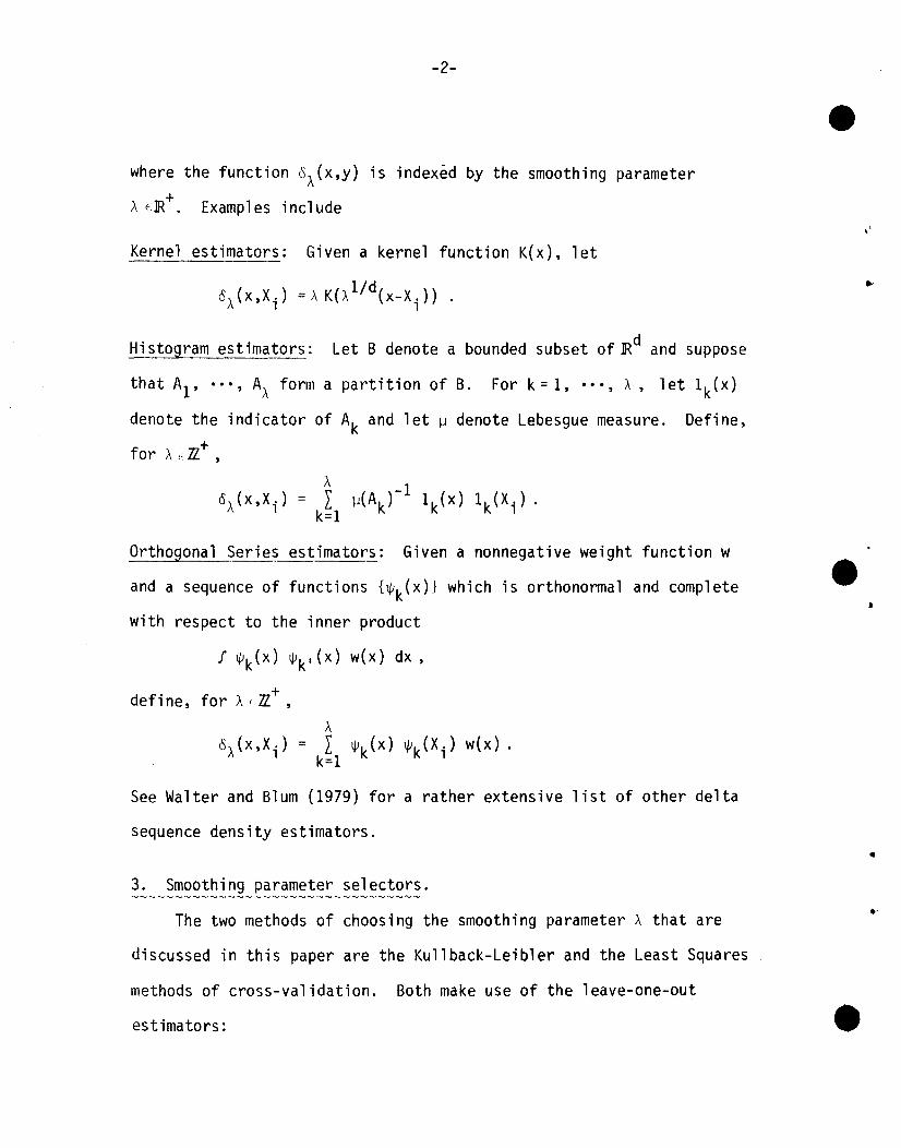
where the function o\(x,y) is indexed by the smoothing parameter

\ FlR+. Examples include

Kernel estimators: Given a kernel function K(x), let

lid0\ (x,X i ) = \ K(\ (x-Xi))

Histogram estimators: Let B denote a bounded subset of lRd and suppose

that AI' ••• , AI.. form a partition of B. For k = 1, ••• , \, let 1k(x)

denote the indicator of Ak and let ~ denote Lebesgue measure. Define,+for \.c ll. ,

\o\(x,X.) = I ~(Ak)-l 1k(X) 1k(X,').

, k=l

Orthogonal Series estimators: Given a nonnegative weight function w

and a sequence of functions {Wk(x)} which is orthonormal and complete

with respect to the inner product

+defi ne, for \ I 7l.. ,

See Walter and Blum (1979) for a rather extensive list of other delta

sequence density estimators.

3. Smoothing parameter selectors.~~ ~· ·v _

The two methods of choosing the smoothing parameter \ that are

discussed in this paper are the Kullback-Leibler and the Least Squares

methods of cross-validation. Both make use of the leave-one-out

estimators:

•

.-

-3-

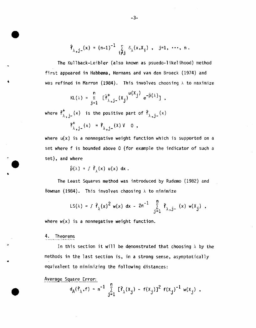
fA . (x) = (n-1 f 1 L (\ (x, X.) , j =1, ••• , n.,J- i,j 1

The Kullback-Leibler (also known as psuedo-likelihood) method

first appeared in Habbema, Hermans and van den Broeck (1974) and

was refined in Marron

nKL (A) = 11

j=1

(1984). This involves choosing A to maximize

u(X.) "()(f~. (X.) J e-PA J,

II ,J- J

,

..

where ~~ . (x) is the positive part of f~ .' (x)II,J- II,J-

~~ . (x) = ~ ~ . (X) V 0,II,J- II.,J-

where u(x) is a nonnegative weight function which is supported on a

set where f is bounded above 0 (for example the indicator of such a

set), and where

P(A) = f 1\ (x) u(x) dx .

The Least Squares method was introduced by Rudemo (1982) and

Bowman (1984). This involves choosing .\ to minimize

A 2 -1 n ~LS(.\) = f f.\(x) w(x) dx - 2n L TA · (x) w(X.) ,

j=l ,J- J

where w(x) is a nonnegative weight function.

4. Theorems

In this section it will be demonstrated that choosing A by the

methods in the last section is, in a strong sense, asymptotically

equivalent to minimizing the following distances:

-4-

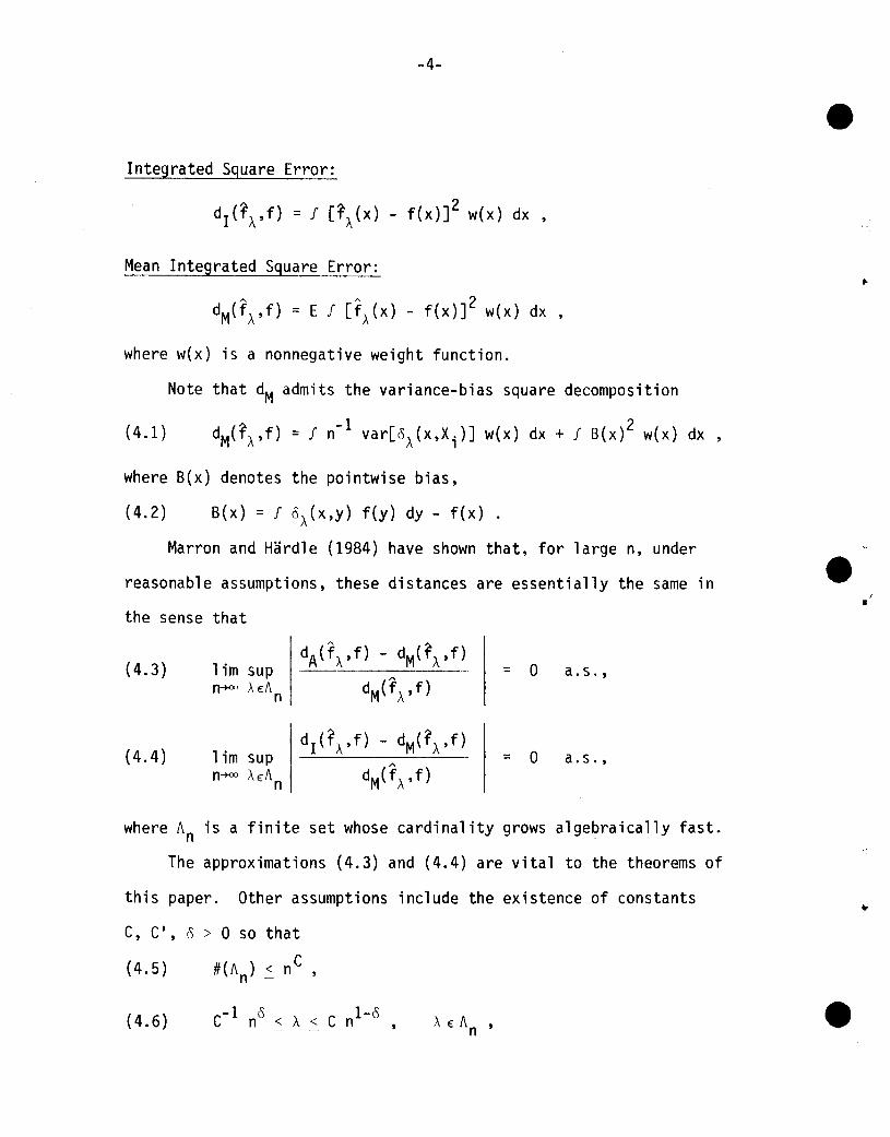
Integrated Square Error:

Mean Integrated Square Error:

where w(x) is a nonnegative weight function.

Note that dMadmits the variance-bias square decomposition

(4.1) dM(~;\,f) = f n- 1 var[o;\(x,X i )] w(x) dx + f B(x)2 w(x) dx ,

where B(x) denotes the pointwise bias,

(4.2) B(x) = f o;\(x,y) f(y) dy - f(x)

Marron and Hardle (1984) have shown that, for large n, under

reasonable assumptions, these distances are essentially the same in

the sense that

..

I•

(4.3)

(4.4)

lim supn~' Af./\

n

dA(fA,f) - dM(~A,f)

dM(fA,f)

dI(fA,f) - dM(~A,f)

dM(fA' f)

= a

= a

a. s. ,

a. s. ,

where An is a finite set whose cardinality grows algebraically fast.

The approximations (4.3) and (4.4) are vital to the theorems of

this paper. Other assumptions include the existence of constants

C, C', °> a so that

(4.5) #(An) ~ nC ,

(4.6)

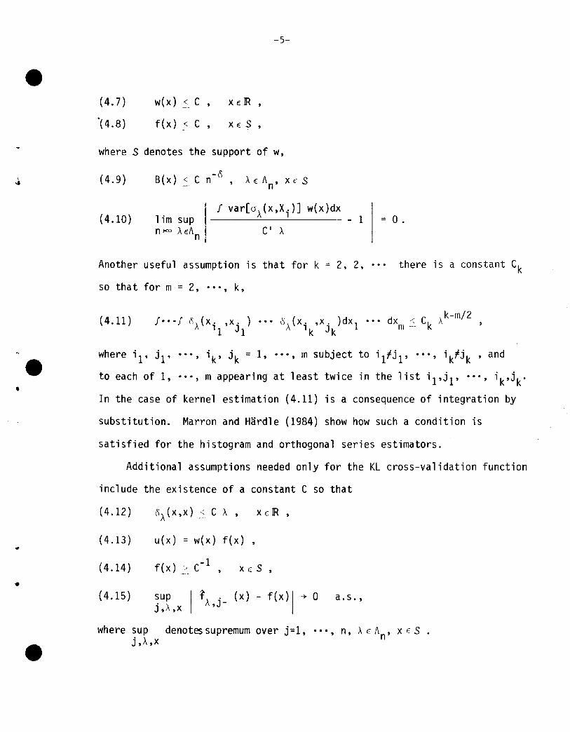
(4.7)

'( 4.8)

w( x) ~_ C, x dR ,

f(x)_~C, XES,

-5-

where S denotes the support of w,

I-a (4.9)

(4.10) lim supn-loOO itEr..n

f var[0It(x,X i )] w(x)dx---------- - 1

C' It= a .

Another useful assumption is that for k = 2, 2, ••• there is a constant Ck

so that for m = 2, "', k,

(4.11)

In the case of kernel estimation (4.11) is a consequence of integration by

substitution. Marron and Hardle (1984) show how such a condition is

•

where iI' jl'

to each of 1,

i k, jk = 1, "', m subject to i 1,jl' "', ik,jk ' and

m appearing at least twice in the list i 1,jl' "', ik,jk'

satisfied for the histogram and orthogonal series estimators.

Additional assumptions needed only for the KL cross-validation function

include the existence of a constant C so that

(4.12) l\ (x,x) _-~ C It , x (. R ,

(4.13) u(x) = w(x) f(x)

(4.14) f(x) -1 XESC ,

(4.15) ~up I ~It '- (x) - f(x) I -+ 0 a. s. ,J,It,X ,J

where sup denotes supremum over j=l, "', n, It E 1\ , XES .. , nJ,I\,X

-6-

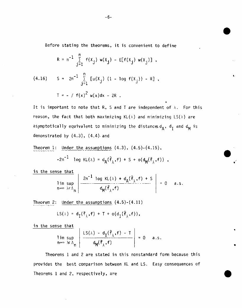
Before stating the theorems, it is convenient to define

1 nR = n- L f(X.) w(X.) - E[f(X

J.) W(XJo)] ,

j=1 J J

(4.16)n

S = 2n-1 j ~1 [u (Xj) (l - 1og f ( Xj )) - R]

T = - f f(x)2 w(x)dx - 2R ...

It is important to note that R, Sand T are independent of A. For this

reason, the fact that both maximizing KL(A) and minimizing LS(A) are

asymptotically equivalent to minimizing the distanc~dA' dI and dMis

demonstrated by (4.3), (4.4), and

Theorem 1: Under the assumptions (4.3), (4.5)-(4.15),

I•in the sense that

lim supn-+<XJ AE f\

n

2n- 1 log KL(A) + dA(fA,f) + S__~ . ~ ",_'0_- __,...__,.. _ .•. _

dM(f\, f)= a a. s.

Theorem 2: Und~_tb~__assumptions. (4.5)- (4.11)

in the sense that

lim supn-+<:o AE f\

n

LS(A) - dI(fA,f) - T

dM(TA,f)= a a. s.

•Theorems 1 and 2 are stated in this nonstandard form because this

provides the best comparison between KL and LS. Easy consequences of

Theorems 1 and 2, respectively, are

-7-

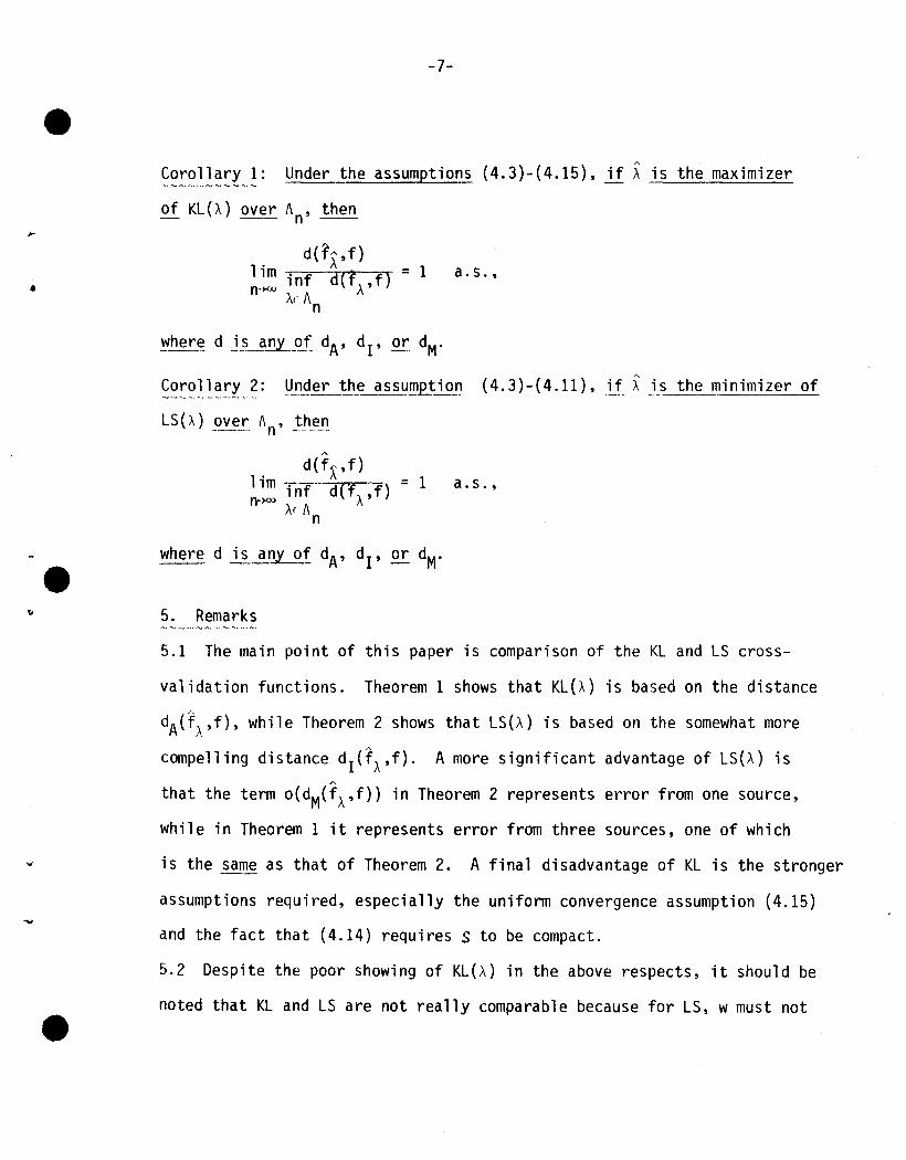
Corollary 1: Under the assumptions (4.3)-(4.15), if ~ is the maximizer

of KL(A) over A , then-- --n--

•a. s. ,

a. s. ,

!Jll~!_~ d j_~~.!!l'..__Qf dA, dI , or. dW

~~~~~.~~~t?: YJ1_~er_th~ssumptio~ (4.3)-(4.11), if ~ is the minimizer of

LS(A)9ve!" "n' _t!l_e_,,!

. d(fA,f)11m Tri1-- d(f, ,f) = 1n->oo Ar" 1\

n

where d is any of dA, dI , or dM.

5. Remarks

5.1 The main point of this paper is comparison of the KL and LS cross­

validation functions. Theorem 1 shows that KL(A) is based on the distance

dA(fA,f), while Theorem 2 shows that LS(A) is based on the somewhat more

compelling distance dI(fA,f). A more significant advantage of LS(A) is

that the term O(dM(fA,f)) in Theorem 2 represents error from one source,

while in Theorem 1 it represents error from three sources, one of which

is the same as that of Theorem 2. A final disadvantage of KL is the stronger

assumptions required, especially the uniform convergence assumption (4.15)

and the fact that (4.14) requires S to be compact.

5.2 Despite the poor showing of KL(A) in the above respects, it should be

noted that KL and LS are not really comparable because for LS, w must not

-8-

depend of f, while for KL, w=u/f, with u independent of f. This is an

advantage of KL because for the important applications of density

estimation to discrimination and to minimum Hellinger distance estimation,

the latter form is more natural.

5.3 The second important point of the results of this paper is that

theoretical backing is given to the idea of Rudemo (1982) to use either

KL or LS for data based comparison of density estimators. For example,

to choose between a kernel and an orthogonal series estimator the one

estimator with the smaller minimum KL(A) (or LS(A)) should have smaller

dA(fA,f) (or dI(fA,f) respectively). Hans-Georg MUller has pointed out

that caution must be used in interpreting these results with respect to

the problem of kernel selection because the asymptotics of this paper do

not properly describe what is happening in that setting. It is conjectured

that Rudemo's idea will also work there.

5.4 As noted in the introduction, the general framework of the results of

this paper contain all or part of the results of a number of recent papers

as special cases. These include the results of Burman (l984), Hall ·(l983a,b),

Marron (1984), and Stone (1984a,b). In most cases the techniques of the

present paper provide a substantical simplification of the proofs in the

earlier papers. Also, the unified approach makes it seem easy to provide

theoretical backing to some interesting heuristics of Bowman, Hall, and

Titterington (1984).

5.5 To save space, some of the assumptions of the theorems of this paper

have been made more restrictive than necessary. For example, (4.5) can

be weakened to 1\n an interval by a straightforward continuity argument

•

"

-9-

(see Hard1e and Marron (1984) for details). The condition (4.6) can also

be substantica11y weakened (compare Burman (1984); Stone (1984a), and

Stone (1984b)). Another straight forward extension is to the case of \

vector or matrix valued as discussed by Oeheuve1s (1977).

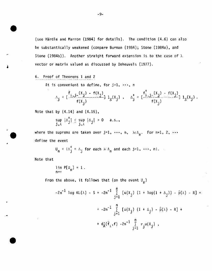
6. Proof of Theorems 1 and 2

It is convenient to define, for j=l •

fA .JX.) - f(X.)/\. = [ ~..J ..J .__L] 1S (Xj )

J f(Xj

)

Note that by (4.14) and (4.15).

~u~ 16;1 ~ ~u~ IAjl + 0 a.S .•J.I\ J.I\

where the suprema are taken over j=l.

define the event

••• , n

n. AE1\n' For n=l. 2. 000

+Un = l/\j = 6j for each ~An and each j=1. nl.

Note that

1im P[Un] = 1 .n--t<Xl

From the above. it follows that (on the event Un)

n-2n- 1 log KL(\) - S = _2n- 1 L [u(X

J.) (1 + 10g(1 + A.)) - p(A) - R] =

j=l J

-1 n= -2n L [u(XJ.) (1 + A

J.) - p(A) - R] +

j=ln

+ dA(f,\,f) _2n- 1 L r.u(X.) •j=l J J

-10-

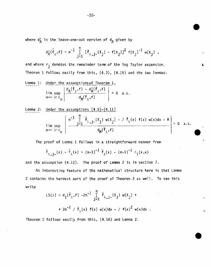
where dA is the 1eave-one-out version of dA given by

n= n- 1 L [1\ .-'X.) - f(X.)]2 f(X.)-l w(X.)

j=l ,J J J J J

and where r j denotes the remainder term of the log Taylor expansion.

Theorem 1 follows easily from this, (4.3), (4.15) and the two lemmas:

~~~~~~,!: Under the assumptionsof Theorem 1,

dA(t,\,f) - dA(f,\,f)1im sup ----------------- = 0 a. s.n-xxo AE1\n dM(1\,f)

- f f,\(x) f(x) w(x)dx - R= a a.s.

f, . (X.) w(X.)/\,J- J J

dM(t,\, f)

Under the assumptions (4.5)-(4.11)n

n- 1 L___j_=1lim sup

n-xx> AE 1\n

Lemma 2:

The proof of Lemma 1 follows in a straightforward manner from

and the assumption (4.12). The proof of Lemma 2 is in section 7.

An interesting feature of the mathematical structure here is that Lemma

2 contains the hardest part of the proof of Theorem 2 as well. To see this

writeA -1 n A

LS(,\) = dI(f,\,f) -2n .I f,\ . (X.) w(X.) +J=1 ,J- J J

+ 2n- 1 f f,\(x) f(x) w(x)dx - f f(x)2 w(x)dx

Theorem 2 follows easily from this, (4.16) and Lemma 2.

)

-11-

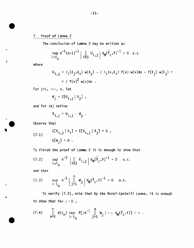
7. Proof of Lemma 2

The conclusion of Lemma 2 may be written as

sup n- 1(n_1)-1 I ~ U.. , dM(f, ,ff1-+ 0 a.s.

, A •. 1,J fIflF. n 1 J

where

Ui,j = ~A(Xj,Xi) w(X j ) - J ~A(x,Xi) f(x) w(x)dx - f(X j ) w(X j ) +

+ J f(x)2 w(x)dx .

For j=l, n, 1et

W. = E[U. ·Ix.],J 1,J J

and for ifj define

Observe that

V.. =U .. -W.1,J 1,J J

e1

(7.1)E[V. ·IX.] = E[V. ·IX.] = 0,

1,J 1 1,J J

E[W j ] = 0 .

To finish the proof of Lemma 2 it is enough to show that

(7.2)

and that

(7.3)

a.s.

a.s.

•To verify (7.3), note that by the Borel-Cantelli Lemma, it is enough

to show that for c > 0 ,

(7.4)

-12-

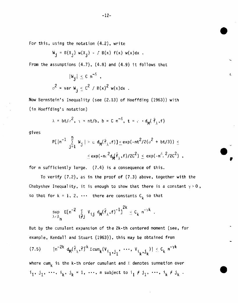
For this, using the notation (4.2), write

From the assumptions (4.7), (4.8) and (4.9) it follows that

IWjl ~ C n-o ,

02

= var W. < C2 f B{x)2 w{x)dxJ -

Now Bernstein's Inequality (see (2.13) of Hoeffding (1963)) with

(in Hoeffding's notation)

2 -I) A

A = bt/o , 1 = nt/b, b = C n ,t = c • dM{ fA ,f)

gives1 n A 2 2

P[ln- j~1 Wj I > L dM{fA,f)J~exp{-nt /2{o + bt/3)) ~.

2 A 2 \ 2 2~exp{-nt: d~fA,f)/2C ) ~ exp{-n l

F /2C ) ,

for n sufficiently large. (7.4) is a consequence of this.

To verify (7.2), as in the proof of (7.3) above, together with the

Chebyshev Inequa1ity, it is enough to show that there is aeons tant y > 0 ,

e•

so that for k = I, 2, there are constants Ck so that

2 A 1 2k -yksup E[n- ~ v.. dM{f"f)- ] ~ Ck n .Ai\. . . , J 1\

en' J

But by the cumulant expansion of the 2k-th centered moment (see, for

example, Kendall and Stuart (1963)), this may be obtained from

(7.5) I -2k A A\' k ( ) I -ykn dM(f,,f) Lcumk V. ., "', V. J' ~. Ck n1\ '1,J 1 'k' k

where cumk is the k-th order cumulant and >: denotes summation over

iI' jl' "', i k, jk = 1, "', n subject to i 1 ; jl' .", i k f jk .

•

-13-

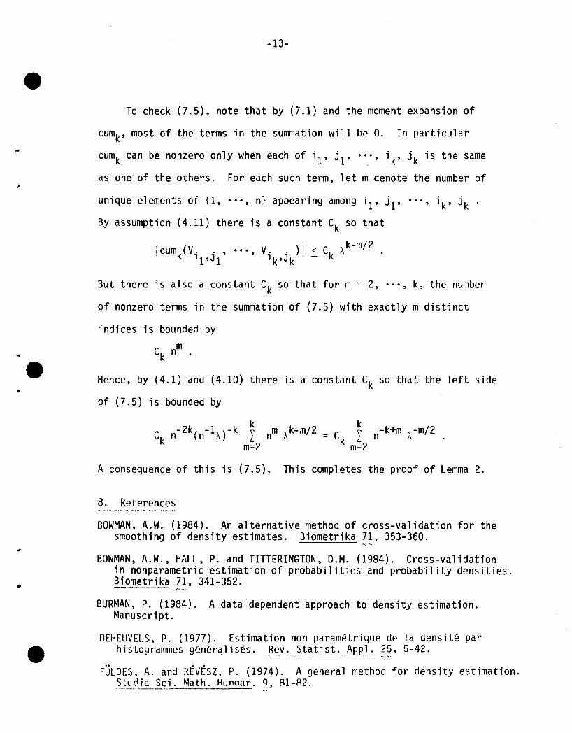
To check (7.5), note that by (7.1) and the moment expansion of

cumk, most of the terms in the summation will be O. In particular

cumk can be nonzero only when each of iI' jl' ••• , i k, jk is the same

as one of the others. For each such term, let m denote the number of

unique elements of {I, ••• , n} appearing among iI' j1'

By assumption (4.11) there is a constant Ck so that

I ( )I k-m/2cumk V. ., •••• V.. < Ck A •'1,J 1 'k·Jk-

But there is also a constant Ck so that for m = 2••••• k. the number

of nonzero terms in the summation of (7.5) with exactly m distinct

indices is bounded by

C nmk

Hence. by (4.1) and (4.10) there is a constant Ck so that the left side

of (7.5) is bounded by

A consequence of this is (7.5). This completes the proof of Lemma 2.

8. References

BOWMAN. A.W. (1984). An alternative method of cross-validation for thesmoothing of density estimates. Biometrika 71. 353-360.

BOWMAN, A.W .• HALL. P. and TITTERINGTON. D.M. (1984). Cross-validationin nonparametric estimation of probabilities and probability densities.Biometrika 71. 341-352 .

BURMAN, P. (1984). A data dependent approach to density estimation.Manuscri pt.

DEHEUVELS, P. (1977). Estimation non parametrique de la densite parhistogrammes generalises. _Rev._~!atis~~]~?~, 5-42.

FULDES. A. and REVESl. P. (1974). A general method for density estimation._~_t~_cl_~S~1. rY1ath. HlJn~ar_. ~. R1-R2.

-14-

HABBEMA, J.D.F., HERMANS, J. and VAN DEN BROEK, K. (1974). A stepwisediscrimination analysis program using density estimation. f~m~~~t

1974: Proceedings in computational statistic~ (G. Bruckman, ed.f101-110. Vienna: Physica Verlag.

HALL P. (1983a). Large sample optimality of least square cross­validation in density estimation. Ann~tatist~ 11, 1156-1174.

HALL, P. (1983b). Asymptotic theory of minimum integrated square errorfor multivariate density estimation. Proc. Sixth_Internat. Symp.Multivariate Anal. Pittsburgh, 25-29.

HARDLE, W. and MARRON, J.S; (1984). Optimal bandwidth selection in non­parametric regression estimation. N.C. Inst. of Statist. Mimeo Series#1546.

HOEFFDING, W. (1963). Probability inequalities for sums of boundedrandom variables. J. Amer. Statist. Assoc. 58, 13-30.

KENDALL, M.G. and STUART, A. (1963). The Advanced Theory of Statistics,Vol. 1: Distribution Theory, Butler and Tanner Ltd.

MARRON, J.S. (1984). An asymptotically efficient solution to the band­width problem of kernel density estimation. N.C. Inst. of Statist.Mimeo Series #1545.

MARRON, J.S. and HARDLE, W. (1984). Random approximations to some measuresof accuracy in nonparametric curve estimation. N.C. Inst. of Statist.Mimeo Series #1566.

RUDEMO, M. (1982). Empirical choice of histogram and kernel densityestimators. Scand. J. Statist. 9, 65-78.

STONE, C.J. (1984a). An asymptotically optimal histogram selection rule.Proceedings of the Berkeley Symposium in Honor of Jerzy Neyman andJack Kiefer II.

STONE, C.J. (1984b). An asymptotically optimal window selection rulefor kernel density estimates. Ann. Stati~~~ ~?, 1285-1297.

WALTER, G. and BLUM, J. (1979). Probability density estimation usingdelta sequences. Ann. Statist. 7, 328-340.

WATSON, G.S. and LEADBETTER, M.R. (1965). Hazard Analysis II. SankhyaA26, 101-116.