Embed Size (px)
Citation preview

JR.S00 1
Lecture 13: (Re)configurable Computing
Prof. Jan Rabaey
Computer Science 252, Spring 2000
The major contributions of Andre Dehon to this slide setare gratefully acknowledged

JR.S00 2
Computers in the News …
TI announces 2 new DSPs
• C64x– Up to 1.1 GHz
– 9 Billion Operations/sec
– 10x performance of C62x
– 32 full-rate DSL modems on a single chip!
• C55x– 0.05 mW/MIPS (20 MIPS/mW!)
– Cut power consumption of C54x by 85%
– 5x performance of C54x
JR.S00 3
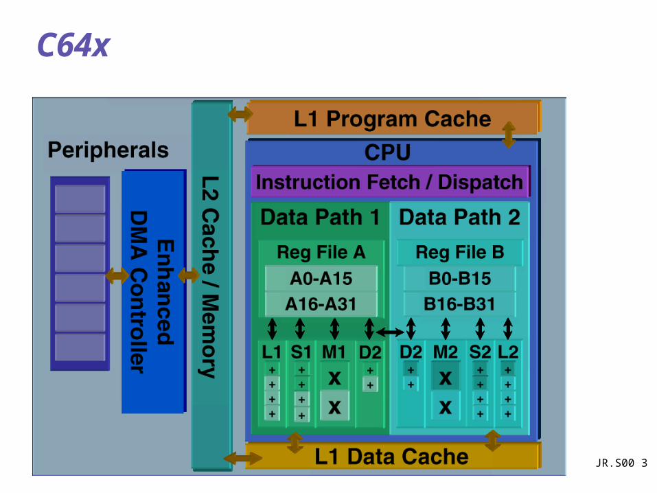
C64x

JR.S00 4
Enhanced performance for communications and multimedia
JR.S00 5
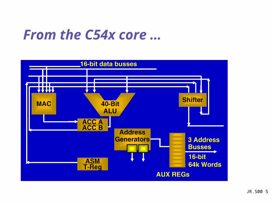
From the C54x core …

JR.S00 6
To the C55x
JR.S00 7
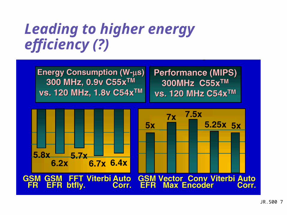
Leading to higher energy efficiency (?)

JR.S00 8
Evaluation metrics for Embedded Systems
Flexibility
Power
Cost
Performance as a Functionality ConstraintPerformance as a Functionality Constraint(“Just-in-Time Computing”)(“Just-in-Time Computing”)
• Components of Cost– Area of die / yield
– Code density (memory is the major part of die size)
– Packaging
– Design effort
– Programming cost
– Time-to-market
– Reusability
JR.S00 9
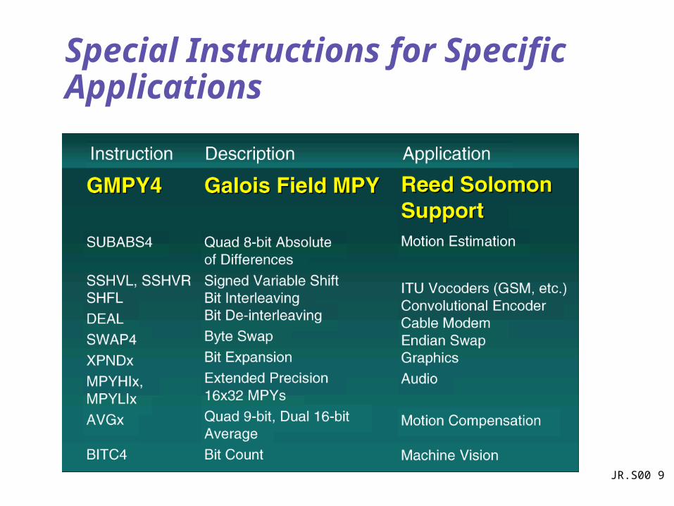
Special Instructions for Specific Applications

JR.S00 10
What is Configurable Computing?
Spatially-programmed connection of Spatially-programmed connection of processing elementsprocessing elements
“Hardware” customized to specifics of problem.
Direct map of problem specific dataflow, control.
Circuits “adapted” as problem requirements change.

JR.S00 11
Spatial vs. Temporal Computing
Spatial Temporal
JR.S00 12
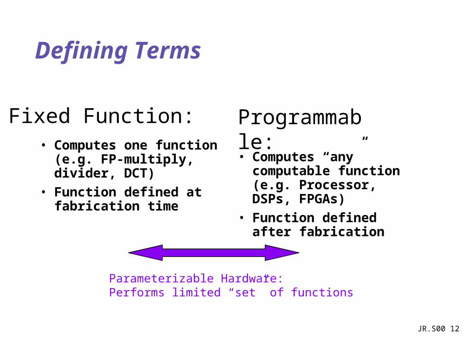
Defining Terms
• Computes one function (e.g. FP-multiply, divider, DCT)
• Function defined at fabrication time
• Computes “any” computable function (e.g. Processor, DSPs, FPGAs)
• Function defined after fabrication
Fixed Function: Programmable:
Parameterizable Hardware:Performs limited “set” of functions
JR.S00 13
“Any” Computation?(Universality)
• Any computation which can “fit” on the programmable substrate
• Limitations: hold entire computation and intermediate data
• Recall size/fit constraint

JR.S00 14
Benefits of Programmable• Non-permanent customization and
application development after fabrication– “Late Binding”
• economies of scale (amortize large, fixed design costs)
• time-to-market (evolving requirements and standards, new ideas)
Disadvantages• Efficiency penalty (area, performance, power)
• Correctness Verification

JR.S00 15
Spatial/Configurable Benefits• 10x raw density advantage over processors
• Potential for fine-grained (bit-level) control --- can offer another order of magnitude benefit
• Locality!
• Each compute/interconnect resource dedicated to single function
• Must dedicate resources for every computational subtask
• Infrequently needed portions of a computation sit idle --> inefficient use of resources
Spatial/Configurable Drawbacks

JR.S00 16
Density Comparison
JR.S00 17
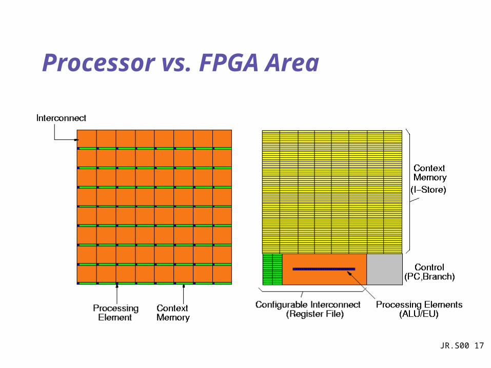
Processor vs. FPGA Area
JR.S00 18
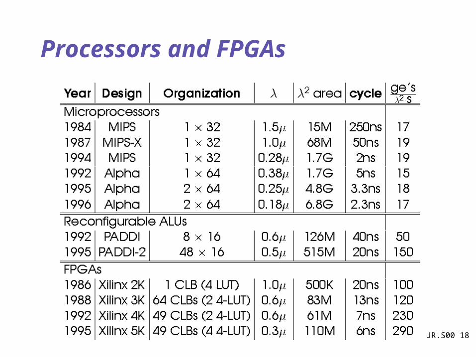
Processors and FPGAs
JR.S00 19
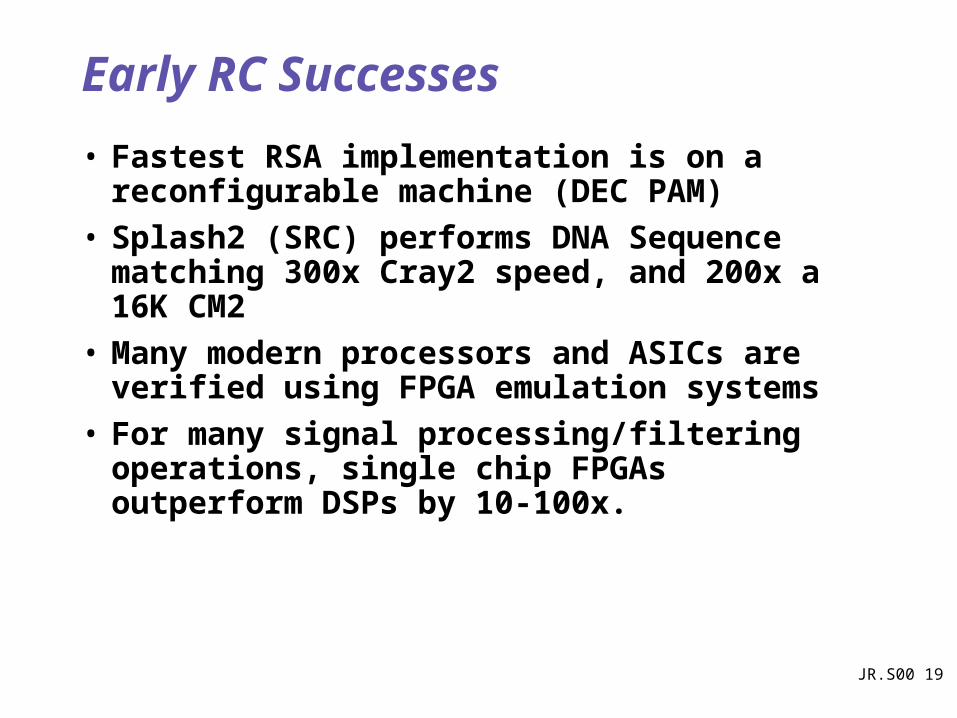
Early RC Successes
• Fastest RSA implementation is on a reconfigurable machine (DEC PAM)
• Splash2 (SRC) performs DNA Sequence matching 300x Cray2 speed, and 200x a 16K CM2
• Many modern processors and ASICs are verified using FPGA emulation systems
• For many signal processing/filtering operations, single chip FPGAs outperform DSPs by 10-100x.

JR.S00 20
Issues in Configurable Design
• Choice and Granularity of Computational Elements
• Choice and Granularity of Interconnect Network• (Re)configuration Time and Rate
– Fabrication time --> Fixed function devices– Beginning of product use --> Actel/Quicklogic FPGAs– Beginning of usage epoch --> (Re)configurable FPGAs– Every cycle --> traditional Instruction Set Processors

JR.S00 21
The Choice of the Computational Elements
ReconfigurableReconfigurableLogicLogic
ReconfigurableReconfigurableDatapathsDatapaths
adder
buffer
reg0
reg1
muxCLB CLB
CLBCLB
DataMemory
InstructionDecoder
&Controller
DataMemory
ProgramMemory
Datapath
MAC
In
AddrGen
Memory
AddrGen
Memory
ReconfigurableReconfigurableArithmeticArithmetic
ReconfigurableReconfigurableControlControl
Bit-Level Operationse.g. encoding
Dedicated data pathse.g. Filters, AGU
Arithmetic kernelse.g. Convolution
RTOSProcess management

JR.S00 22
FPGA Basics
• LUT for compute
• FF for timing/retiming
• Switchable interconnect
• …everything we need to build fixed logic circuits
– don’t really need programmable gates
– latches can be built from gates

JR.S00 23
Field Programmable Gate Array (FPGA) Basics
Collection of programmable “gates” embedded in a flexible interconnect network.
…a “user programmable” alternative to gate arrays.
?Programmable Gate

JR.S00 24
Look-Up Table (LUT)
In Out00 001 110 111 0
2-LUT
Mem
In1 In2
Out
JR.S00 25
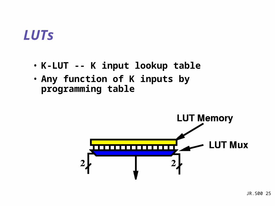
LUTs
• K-LUT -- K input lookup table
• Any function of K inputs by programming table

JR.S00 26
Conventional FPGA Tile
K-LUT (typical k=4) w/ optional output Flip-Flop

JR.S00 27
Commercial FPGA (XC4K)
• Cascaded 4 LUTs (2 4-LUTs -> 1 3-LUT)
• Fast Carry support
• Segmented interconnect
• Can use LUT config as memory.

JR.S00 28
XC4000 CLB

JR.S00 29
Not Restricted to Logic GatesExample: Paddi-2 (1995)
EXU
FSM
IME
M
EXU
FSMIM
EM
EXU
FSM
IME
M
EXU
FSM
IME
M
EXU
FSM
EXU
FSM
EXU
FSM
EXU
FSM
IME
M
COMMUNICATION NETWORK
IME
M
IME
M
IME
M
nanoprocessor

JR.S00 30
A Data-driven Computation Paradigm
Interconnection Network
in1 out
EXU
in2
pos? +1
sel
PE1 PE2 PE3
CTRL
EXU
CTRL
EXU
CTRL
in1 in2
out

JR.S00 31
Not restricted to Logic Gate Operations

JR.S00 32
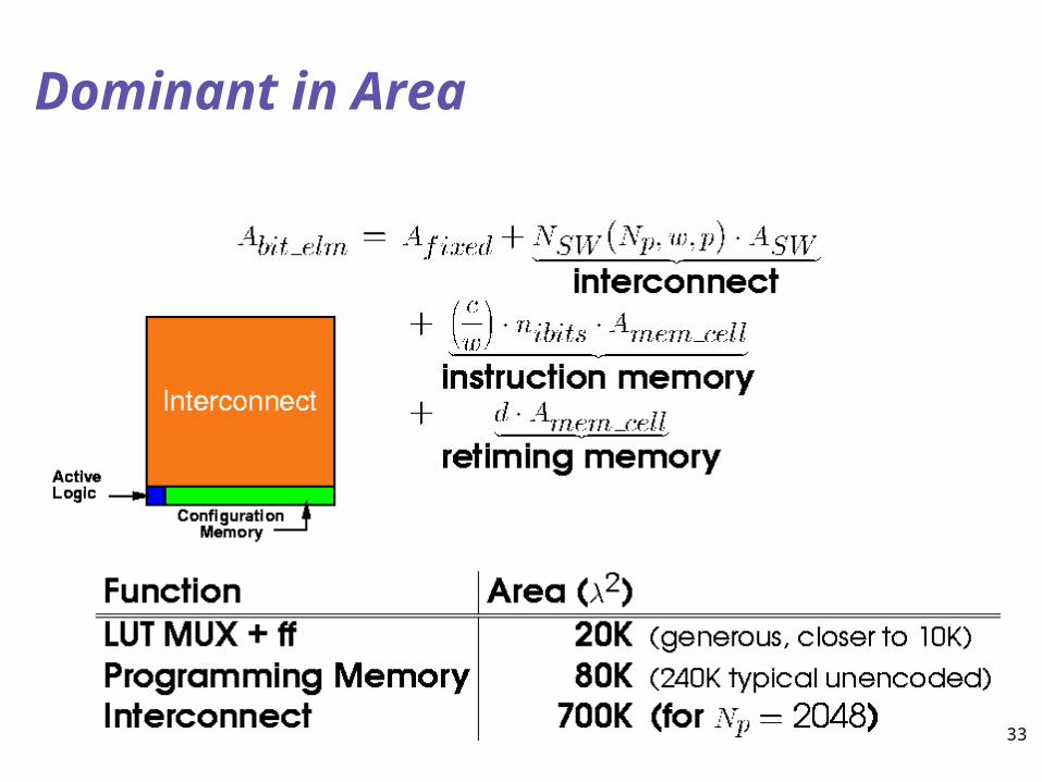
For Spatial Architectures
• Interconnect dominant– area
– power
– time
• …so need to understand in order to optimize architectures
JR.S00 33
Dominant in Area

JR.S00 34
Dominant in Time
JR.S00 35
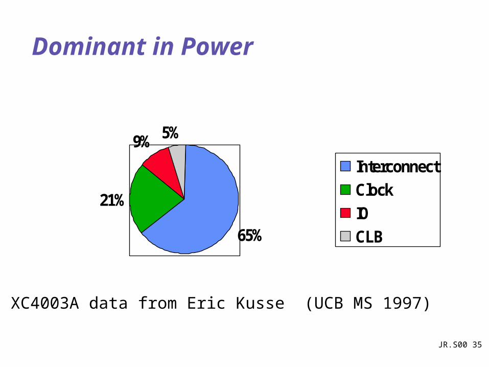
Dominant in Power
65%
21%
9% 5%
Interconnect
Clock
IO
CLB
XC4003A data from Eric Kusse (UCB MS 1997)

JR.S00 36
Interconnect
• Problem– Thousands of independent (bit) operators producing
results
» true of FPGAs today
» …true for *LIW, multi-uP, etc. in future
– Each taking as inputs the results of other (bit) processing elements
– Interconnect is late bound
» don’t know until after fabrication
JR.S00 37
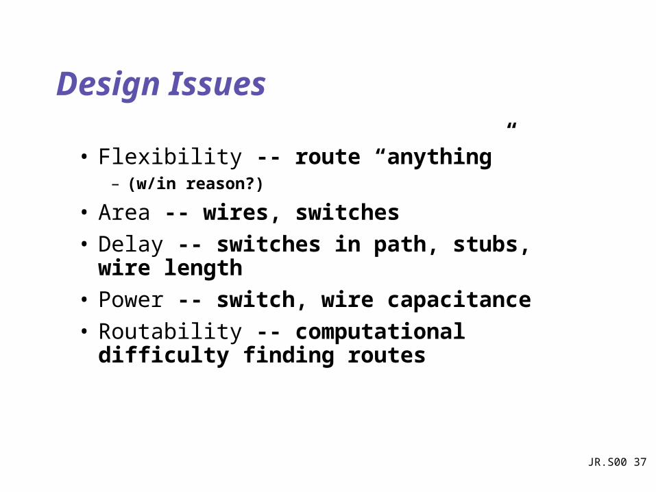
Design Issues
• Flexibility -- route “anything” – (w/in reason?)
• Area -- wires, switches
• Delay -- switches in path, stubs, wire length
• Power -- switch, wire capacitance
• Routability -- computational difficulty finding routes
JR.S00 38
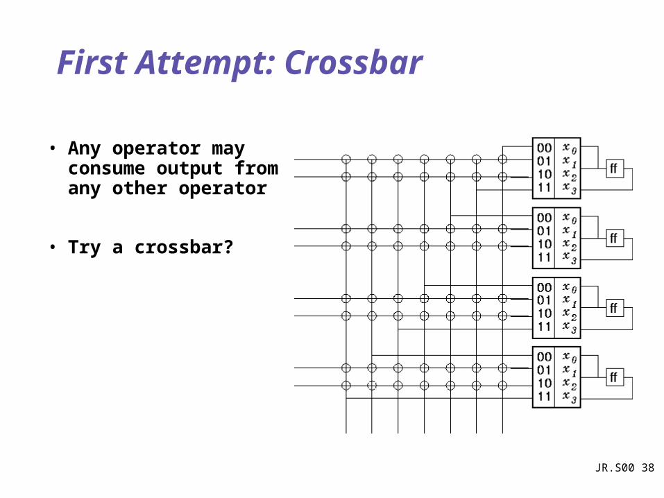
First Attempt: Crossbar
• Any operator may consume output from any other operator
• Try a crossbar?

JR.S00 39
Crossbar
• Flexibility (++)– routes everything
(guaranteed)
• Delay (Power) (-)– wire length O(kn)
– parasitic stubs: kn+n
– series switch: 1
– O(kn)
• Area (-)– Bisection bandwidth n
– kn2 switches
– O(n2)
Too expensive and not scalable
JR.S00 40
Avoiding Crossbar Costs
• Good architectural design– Optimize for the common case
• Designs have spatial locality
• We have freedom in operator placement
• Thus: Place connected components “close” together
– don’t need full interconnect?

JR.S00 41
Exploit Locality• Wires expensive
• Local interconnect cheap
• Try a mesh?LUT
C BoxS Box

JR.S00 42
The Toronto ModelSwitch Box
Connect Box
JR.S00 43
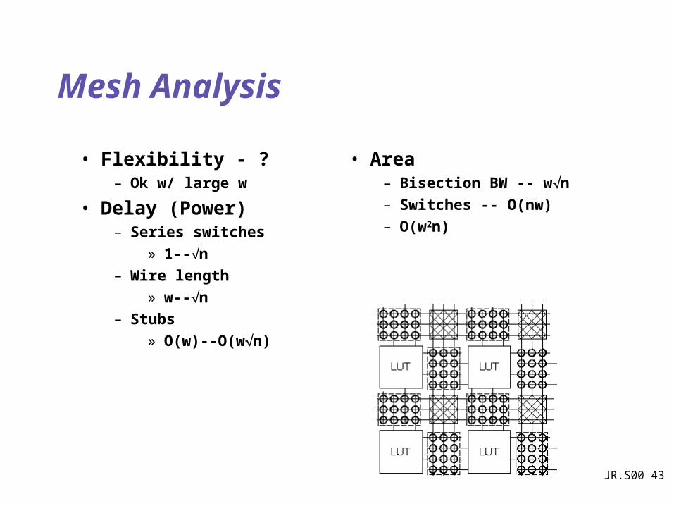
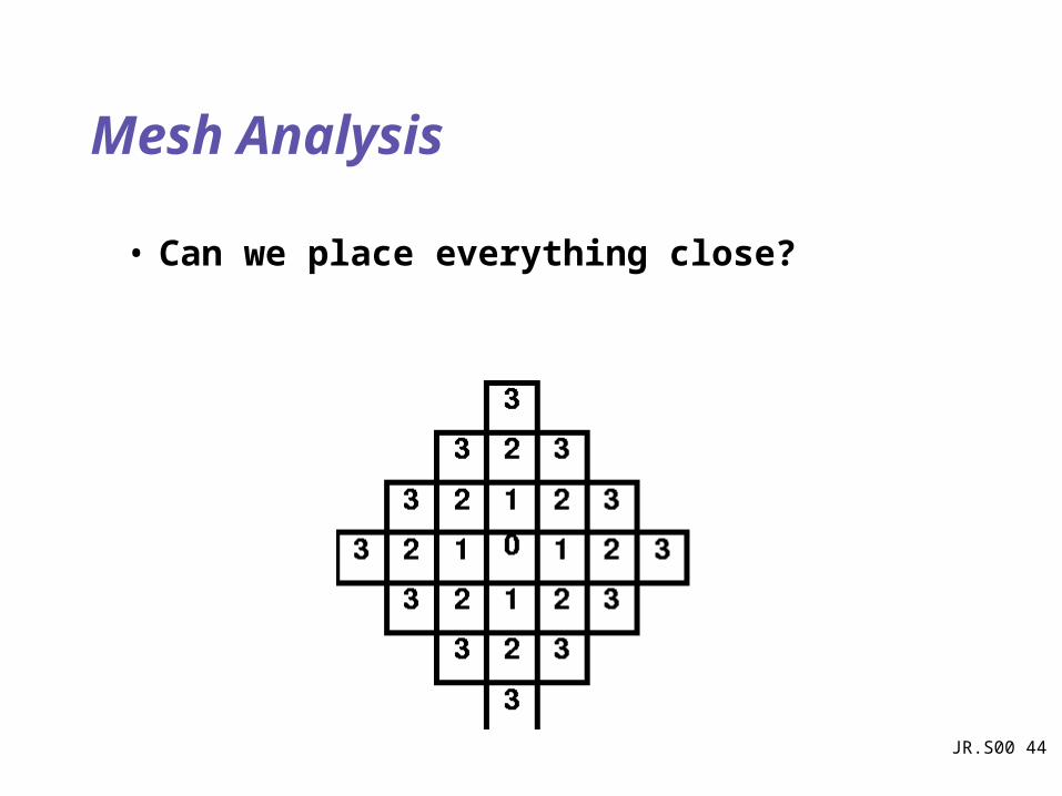
Mesh Analysis
• Flexibility - ?– Ok w/ large w
• Delay (Power)– Series switches
» 1--n
– Wire length
» w--n
– Stubs
» O(w)--O(wn)
• Area– Bisection BW -- wn
– Switches -- O(nw)
– O(w2n)
JR.S00 44
Mesh Analysis
• Can we place everything close?

JR.S00 45
Mesh “Closeness”
• Try placing “everything” close

JR.S00 46
Adding Nearest Neighbor Connections
• Connection to 8 neighbors
• Improvement over Mesh by x3
Good for neighbor-neighbor connections

JR.S00 47
Typical Extensions
• Segmented Interconnect
• Hardwired/Cascade Inputs

JR.S00 48
XC4K Interconnect

JR.S00 49
XC4K Interconnect Details

JR.S00 50
Creating HierarchyExample: Paddi-2
Network
P1P2P3P4
P5P6P7P8
P9P10P11P12
P13P14P15P16
P17P18P19P20
P21P22P23P24
P25P26P27P28
P29P30P31P32
P33P34P35P36
P37P38P39P40
P41P42P43P44
P45P46P47P48
brea
k-s
wit
ch
brea
k-s
wit
ch
I/O I/O I/O I/O
16 x 6
Level-2
16 x 16b
I/O I/O I/O I/O
switch matrix
NetworkLevel-1
6 x 16b

JR.S00 51
Level-1 Communication Network
P0
P1
P2
P3
ControlData
• 1-cycle Latency
• Full Connectivity
• On top of Data Path in Metal-2
JR.S00 52
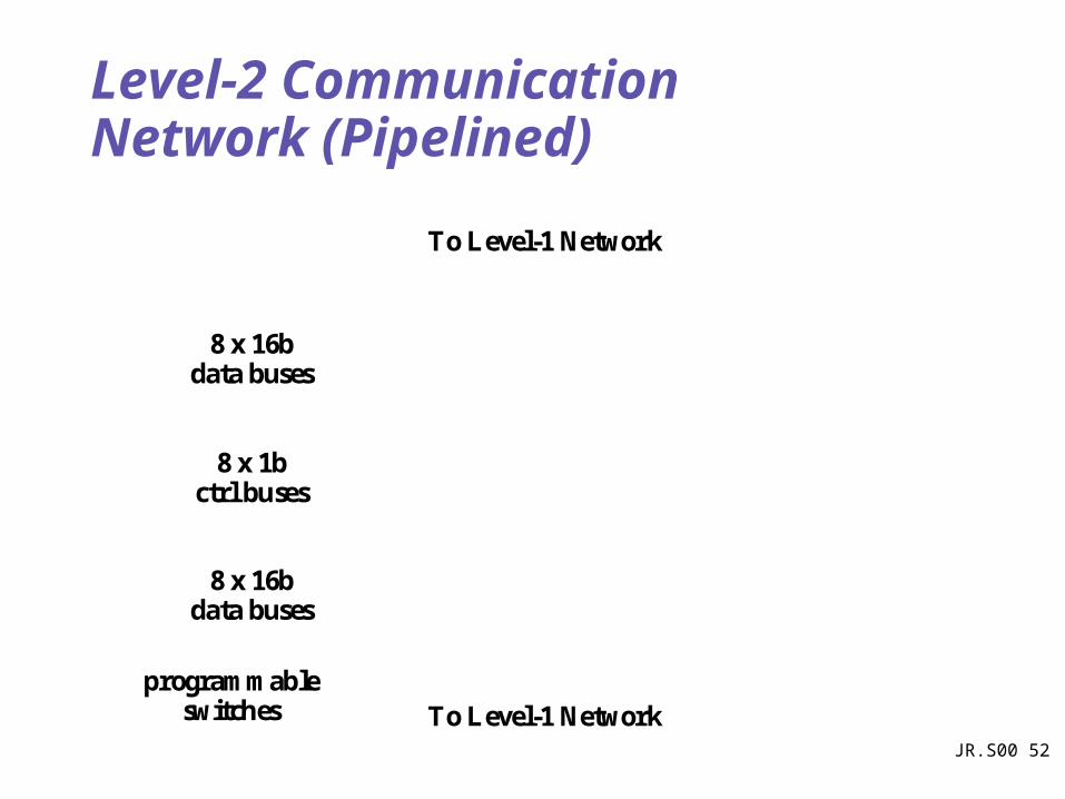
Level-2 Communication Network (Pipelined)
8 x 16b data buses
To Level-1 Networkprogrammable
switches
8 x 16b data buses
8 x 1bctrl buses
To Level-1 Network

JR.S00 53
Paddi-2 Processor
• 1-m 2-metalCMOS tech
• 1.2 x 1.2 mm2
• 600k transistors
• 208-pin PGA
• fclock = 50 MHz
• Pav = 3.6 W @ 5V
JR.S00 54
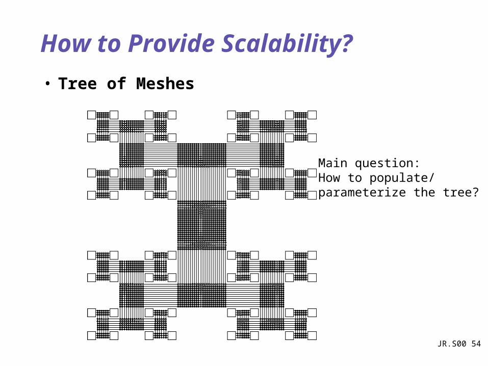
How to Provide Scalability?
• Tree of Meshes
Main question: How to populate/parameterize the tree?

JR.S00 55
Hierarchical Interconnect
• Two regions of connectivity lengths
Manhattan Distance
Ene
rgy
x D
elay
Mesh
Binary Tree
• Hybrid architecture using both Mesh and Binary structures favored

JR.S00 56
Hybrid Architecture Revisited
Straightforward combination of Mesh and Binary tree is not smart
• Short connections will be through the Mesh architecture
• The cheap connections on the Binary tree will be redundant

JR.S00 57
Inverse Clustering
• Blocks further away are connected at the lowest levels
• Inverse clustering complements Mesh Architecture
Manhattan Distance
Ene
rgy
x D
elay
Mesh
Binary Tree
Mesh + Inverse
JR.S00 58
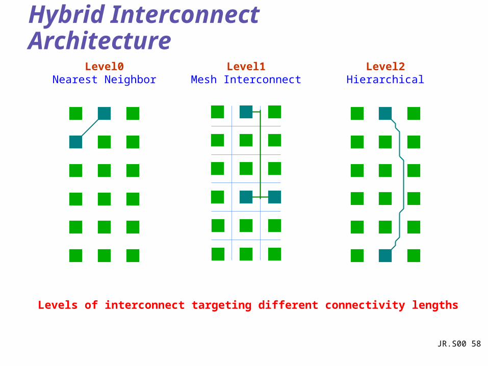
Hybrid Interconnect Architecture
Levels of interconnect targeting different connectivity lengths
Level0Nearest Neighbor
Level1Mesh Interconnect
Level2Hierarchical

JR.S00 59
Prototype
• Array Size: 8x8 (2 x 4 LUT)
• Power Supply: 1.5V & 0.8V
• Configuration: Mapped as RAM
• Toggle Frequency: 125MHz
• Area: 3mm x 3mm
• Process: 0.25U ST
JR.S00 60
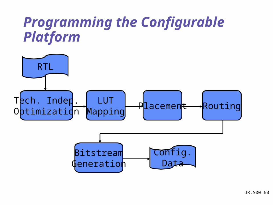
Programming the Configurable Platform
LUTMapping
Placement Routing
BitstreamGeneration
Tech. Indep.Optimization
Config.Data
RTL

JR.S00 61
Starting Point
• RTL– t=A+B
– Reg(t,C,clk);
• Logic– Oi=AiiCi
– Ci+1 = AiBiBiCiAiCi

JR.S00 62
LUT Map

JR.S00 63
Placement
• Maximize locality– minimize number of wires in each channel
– minimize length of wires
– (but, cannot put everything close)
• Often start by partitioning/clustering
• State-of-the-art finish via simulated annealing

JR.S00 64
Place

JR.S00 65
Routing
• Often done in two passes– Global to determine channel
– Detailed to determine actual wires and switches
• Difficulty is – limited channels
– switchbox connectivity restrictions

JR.S00 66
Route

JR.S00 67
Summary
• Configurable Computing using “programming in space” versus “programming in time” for traditional instruction-set computers
• Key design choices– Computational units and their granularity
– Interconnect Network
– (Re)configuration time and frequency
• Next class: Some practical examples of reconfigurable computers


![Computer Engineering BSE André DeHon [ESE] (CEPC Chair) andre@seas.upenn.edu](https://img.pdfslide.us/doc/110x75/56649d0c5503460f949e0fd1/computer-engineering-bse-andre-dehon-ese-cepc-chair-andreseasupennedu.jpg)

![[Jan M. Rabaey, Massoud Pedram] Low-Power-Design-M(Bookos.org)](https://img.pdfslide.us/doc/110x75/55cf9cda550346d033ab4ad0/jan-m-rabaey-massoud-pedram-low-power-design-mbookosorg.jpg)