Journal of the © 1961 The Operations Research Society of ...archive/pdf/e_mag/Vol.04_04_135.pdfOperations Research Society of Japan VOLUME 4 July 1962 NUMBER 4 -----ON THE ECONOMICAL

Journal of the Operations Research Society of Japan

VOLUME 4 July 1962 NUMBER 4 -----------------

ON THE ECONOMICAL ASSIGNMENT OF COMPONENT TOLERANCES

NORIHIRO YAMAKA W A

Kasado Works, Hitachi Ltd. (Received Feb. 24, 1962)

1. INTRODUCTION

The problem considered is that of how to select component tolerances so as to minimize production costs--assuming a situation in which the product is assembled from a number of component parts. Several approaches have been made to this problem in the recent years (e. g. Taguchi [lJ and Evans [2]). In this paper, the author, taking several assumptions for granted, proposes a graphical solution of this problem by means of an iterative scheme. The three assumptions taken here are as follows:

1) All component parts are under statistical control; 2) The statistical behavior of the component response can be esti

mated as a function of the component's production cost; and 3) The production cost of the assembled product can be estimated

as the sum of the production costs of component parts.

2. MATHEMATICAL FORMULATION OF THE PROBLEM

Let us suppose that the principal response y of the assembled product can be represented as a function of the responses xi's Ci=l, 2, ...... , n) of its component parts. Let us also assume that Xi can be measured by the deviation from the center of tolerance of Xi.

(1)

135

© 1961 The Operations Research Society of Japan

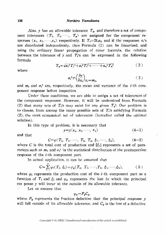
136 Norihiro Yamakawa

Also, Y has an allowable tolerance Ty, and therefore a set of component tolerances (Tl , T 2, .. ····, T",) are assigned for the component responses (Xl, X2, .. ····,Xn) respectively. If T i =2fi (Ji, and if the responses xi's

are distributed independently, then Formula (1) can be linearized, and using the ordinary linear propagation of error formula, the relation between the tolerance of y and Tt's can be expressed in the following formula

(2)

where

(3)

and mi and (Ji2 are, respectively, the mean and variance of the i-th component response before inspection.

Under these conditions, we are able to assign a set of tolerances of the component responses. However, it will be understood from Formula (2) that many sets of Ti's may exist for any given T/. Our problem is to choose, from among the many possible sets of Tt's satisfying Formula (2), the most economical set of tolerances (hereafter called the optimal solution).

In this type of problem, it is necessary that Y=Y(Xl, X2, .. ····, xn)

and that (4-1)

C=fjJ(TJ, T 2,······, Tn, Ty, ~l,······, ~n), (4-2)

where C is the total cost of production and {~tl represents a set of parameters such as mi and (Ji2 in the statistical distribution of the preinspection response of the i-th component part.

In actual application, it can be assumed that

" C= L fjJi(Ti , ~i)+fjJy(Ty, TJ,······, Tn, ~l, .. ····'~n)' (5) i~l

where fjJl represents the production cost of the i-th component part as a function of Ti and ~i and fjJy represents the loss fo which the principal res ponse Y will incur at the outside of its allowable tolerance.

Let us assume that fjJy=PyCy,

where P y represents the fraction defective that the principal response Y will fall outside of its allowable tolerance, and Cy is the loss of a defective

Copyright © by ORSJ. Unauthorized reproduction of this article is prohibited.

Economical Assignment of Component Tolerances 137

assembly. If Cv can be assumed to be a constant, and if it can be assumed that y is distributed according to a normal distribution, then the mean my and the variance uy2 can be calculated from the following transformations,

(6-1) and

(6-2) where k is the normalized variate of y, and k[ and k2 represent the lower and upper limits, respectively, of the normalized tolerance of y.

and

The my and uy2 are also determined by the following relations 11

uy2= ~ aiu/2

i~l (7-1)

my=y(m[', rn2',······,mn'), (7-2)

where m/ and u/2 represent, respectively, the mean and variance of the Xi of acceptable products.

We can say, therefore, that our problem consists with to select the component tolerance so as to minimize production cost

" 9= L 1f;(Ti , ~i) i~l

-subject to restraints on Formula (7), where

~i= (mi, Ui2)

and

lx ••

u/2= (xi- m /)2fi(Xi)dxi, x,.

(8)

(9-1)

(9-2)

(9-3)

is the pdf of the i-th final acceptable component response, and Xli and Xu are the lower and upper allowable limits of the i-th component response.

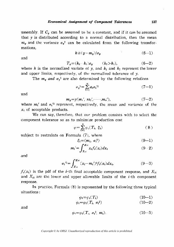
In practice, Formula (8) is represented by the following three typical situations:

.and

9i=(ptCTi)

9i=9i(Ti' U(2)

(10-1) (10-2)

(10-3)


138

(/)

Norihiro Yamakawa

The first one of these (10-1) has been solved by G. Taguchi under the following assumption

CPi= f,l T.)-a,

X-ilr )(.1.2 ---->;.I

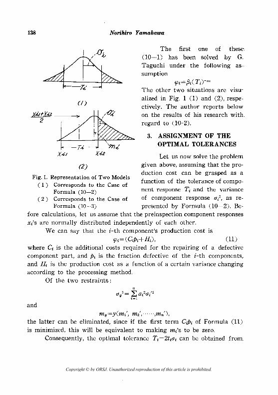
The other two situations are visualized in Fig. 1 (1) and (2), respectively. The author reports below on the results of his research with regard to (10-2). 2

X~/

(2)

3. ASSIGNMENT OF THE OPTIMAL TOLERANCES

Fig. 1. Representation of Two Models ( 1) Corresponds to the Case of

Formula (10-2)

Let us now solve the problem given above, assuming that the production cost can be grasped as a function of the tolerance of component response Ti and the variance of component response al, as represented by Formula (10-2). Be-

( 2) Corresponds to the Case of Formula (10-3)

fore calculations, let us assume that the preinspection component responses x/s are normally distributed independently of each other.

We can say that the i-th component's production cost is

CPi= (CPi+ Hi), (11) where Ci is the additional costs required for the repairing of a defective component part, and Pi is the fraction defective of the i-th components, and 1ft is the production cost as a function of a certain variance changing according to the processing method.

Of the two restraints:

" a/= Lai2a/2 i=1

and my=y(m/, m2',····· ·,mn'),

the latter can be eliminated, since if the first term CiPi of Formula Cll} is minimized, this will be equivalent to making m/s to be zero.

Consequently, the optimal tolerance Ti=2tiai can be obtained from



the solution of the following simultaneous equations a '

a4(¥'+Aa/)=O I

a I' aa/¥'+Aa/)=O ,I

(12)

where A is the Lagrange multiplier. Now, if f(t) is taken to be the pdf of the component response be-

fore inspection, then

and

It,

Pi=l- f(t)dt=PCti) -t,

Furthermore we can put H,= {3i(at2 )-a,

where at and {3t represent parameters with respect to several conditions for the i-th component part. This results in

~~ ~O (tt~OO), apt aat_ -'- 0 aH

t""\"" .

Then, from Formula (12) we obtain a

aPt (¥'+Aat/) =0

We then obtain

Here, denoting as

we finally obtain

a~(¥'+Aa,/)=O

Ct+,(a~~ [~a/at2kCti) ] =0

1+,( a~i[ ~ai2(]t2kCti) ] =0

(13)

(14)

(15) controlling

(16)

(17)

(18)



A~,=Cda,: } . Aq>,=[3da,

(19)

Consequently, we are able to determine the optimal set of tolerances of component responses (t1, f 2,···· ',fn ; (11, (12,.··· ··,(In). The i-th tolerance Tt can be calculated from T i=2fi(li. The solution of Formula (19) is. obtained from the intersection of curve cp, and the other curve 1>, on the graph representing the optimal relations between kCti) and (li2•

4. ITERATIVE SCHEME

4. 1. Calculation of CPi and 1>i In order to establish an iterative scheme, it is necessary to calculate·

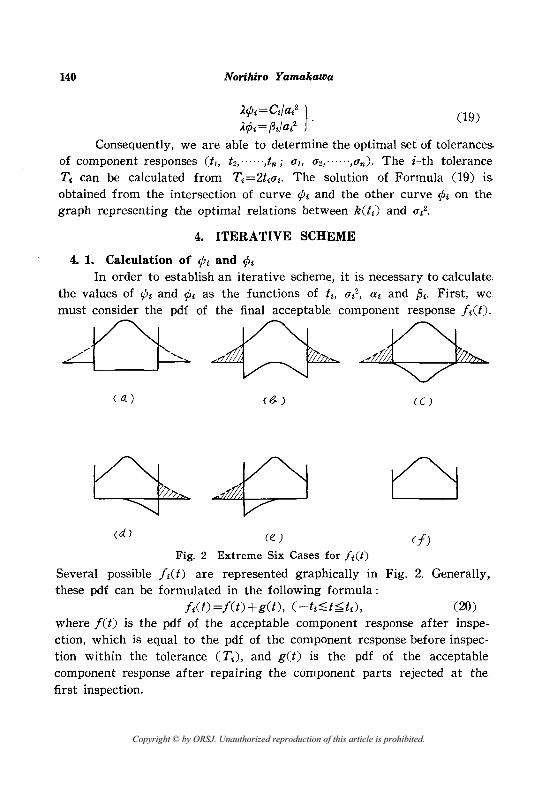
the values of CPi and 1>t as the functions of ti, (li2, at and [3i. First, we must consider the pdf of the final acceptable component response li(t).

~ odV CC)

Cd) (e)

Fig. 2 Extreme Six Cases for f,Ct)

Several possible li(t) are represented graphically in Fig. 2. Generally r

these pdf can be formulated in the following formula: It(t)=/(t)+g(t), (-t,-:;;.t-:;;.tt), (20)

where l(t) is the pdf of the acceptable component response after inspection, which is equal to the pdf of the component response before inspection within the tolerance (Ti ), and get) is the pdf of the acceptable component response after repairing the component parts rejected at the first inspection.


Economical ABBignment of Component ToleranceB 141

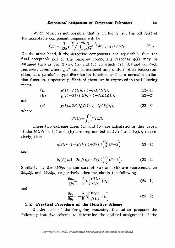
When repair is not possible, that is, in Fig. 2 Ce), the pdf I;Ct) of the acceptable component response will be

1 t'/lt. 1 t' I;Ct) = ~21/ -2 _t.';2;~e-2 dt, C -t;?t?t;). (21)

On the other hand, if the defective components are repairable, then the final acceptable pdf of the repaired component response gCt) may be assumed such as Fig. 2 Ca), Cb) and Cc), in which Ca), Cb) and (c) each represent cases where gCt) can be assumed as a uniform distribution function, as a parabolic type distribution function, and as a normal distribution function, respectively. Each of them can be expressed in the following terms

and

where

Ca) Cb)

(c)

gCt) = FCt;)/t; (--t;?t?t;), gCt)=3FCttW/t;3 C -t;?t?tD,

FCt;) =100 ICt)dt. t,

C22-1) C22-2)

(22-3)

These two extreme cases Ca) and Cb) are calculated in this paper. If the kCt;)'s in (a) and Cb) are represented as kaCt;) and kb(t;), respectively, then

(23-1)

and

(23-2)

Similarly, if the ak/ap; in the case of (a) and (b) are represented as aka/aPt and akb/ap;, respectively, then we obtain the following

~~:=-}t{jg~?+t;] C24-1)

and

akb=_~t 1-£Ct;2+t ] apt 5 i J(t,D ;, C24-2)

4. 2. Practical Procedure of the Iterative Scheme On the basis of the foregoing reasoning, the author proposes the

following iterative scheme to determine the optimal assignment of the



set of tolerance of the component responses. Cl) Basic Data to be Prepared

Ca) The tolerance to be given for the response of the given assembly; Ty

Cb) The allowable ratio for the principal response falling outside the assembly tolerance Ty; Py

Cc) The relation between the principal response y and the component responses (Xl, X2,······, Xn) ;

Y=Y(Xl,tX2,' ..... , xn)

Cd) The additional cost required for repairing one defective component part: Ct

Ct is assumed to vary according to the component response number (i)but to be a constant not effected by tt and at.

(e) The two parameters at and fit in the relation between the production cost and the variance of the component response;

lft= fit/(anal It may also be possible that there are parts for which any other

production method would be unconsiderable, for instance, when there is only one suitable type of tool. In these cases, the data here is not required, and it is sought from the constant at2 as a function of cj;t alone.

(2) Computation Procedure (a) Compute the at2 from

( §L)2 =at2 aXt ",,~m. .

Cb) Using the given Ty and Py and the normal distribution table, compute the k of 11= -~ ./271: k e 2 dt=Py/2

and compute a,/ from

~y =kqy.

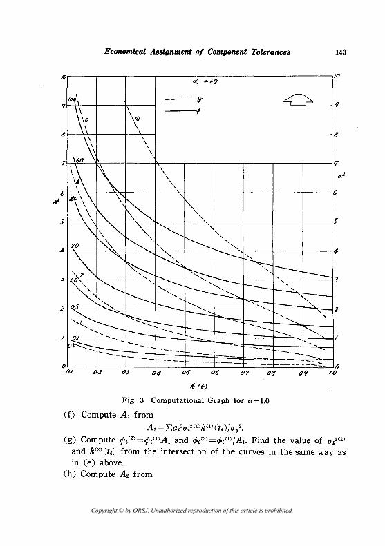
(c) Compute cj;/D =Ct/al and cftt(1) = fit/al. Cd) Select the computation graph (refer to Fig. 3) for the at of the

given component part. Ce) Find the value of al(1) and k(1)(tt) from the intersection of the

curves cj;t(1) and cftt(l) in Figure (d) calculated at step Cc).



o 1 01. =<-;'0

10f.\ ------11' ~

~t \ f \ vo

\ \

\60~\ \

\ \

8

6

\~ \ \ \

\

" 4\<\ \ ,

\ ~ I"'" ~ , '\ ~~ ',,- ~ " ,

20 ~ ~" , ........... -- "'"

\~ '" ~ ~ ~ ~ ~~

, I---r--" "

~ ~ ",,~ '- --- "

I'-- r--- '-.... , ~ ..,., ~

-",-", I--

, f-- " /).r; ......

,)-......... ~ --.::::.::, ..... , ~

, ..... " - , ..... , ..... :-- r.::::- ---t--- -- -- ----- ", --~~ -- - ..... ---- -- - -I---- - -- --- '- -- -- ---- --t- t- t- - ----~---- - -::::.

6

s s

4 4

3

2

;. I

-o ()./ tJ-2 {)J tJ4 os tJ·., tJ8 tJ·9

() /.Q

~ (t)

Fig. 3 Computational Graph for a=LO

(f) Compute Al from

Al = L:.ala/(1)k(l) (ti)/a,}.

(g) Compute rjJ/2)=rjJi(l)A I and rp/2) = (/>i(l)/A I • Find the value of a,2(2) and k(2)(ti ) from the intersection of the curves in the same way as in (e) above.

(h) Compute A2 from


144

/·0

0·[5

07

het)

().6

(J5

(}-J

02

(j·1

o

Norihiro Yamakawa

~ I-

~ ~

~ V

[7; V

j V ~ i-V/

/ if I1 /

I / I1 I

/ / f if

I1 I I /

1 I1 I1 I

/ '/ 7) //

/;V ~ V

/ 2

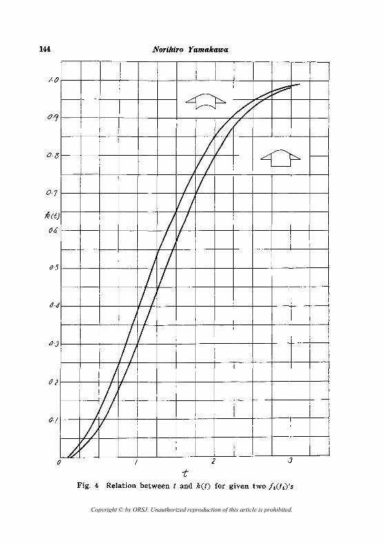
Fig. 4 Relation between t and k(t) for given two 11.(tl,)'s



n

A2 = L. ai2a/2)k(2) Cti)/ay2. i-I

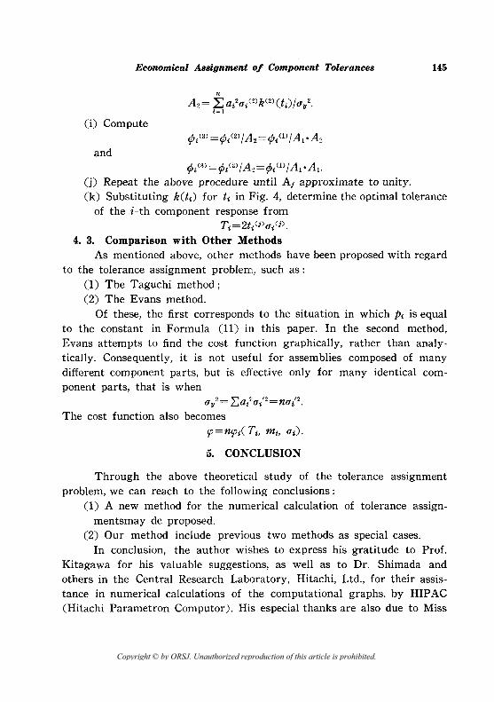
(i) Compute

and ifJ/3) = ifJ/2) / A2 = ifJ/1) / Al· Al.

(j) Repeat the above procedure until Aj approximate to unity. (k) Substituting kCti) for tt in Fig. 4, determine the optimal tolerance

of the i-th component response from T t =2l,(j)ai(j).

4. 3. Comparison with Other Methods As mentioned above, other methods have been proposed with regard

to the tolerance assignment problem, such as: (1) The Taguchi method; (2) The Evans method.

Of these, the first corresponds to the situation in which Pi is equal to the constant in Formula (11) in this paper. In the second method, Evans attempts to find the cost function graphically, rather than analytically. Consequently, it is not useful for assemblies composed of many different component parts, but is effective only for many identical component parts, that is when

a/= 'L.a/a/2=na/2. The cost function also becomes

rp=nrpt(Ti , mi, at).

5. CONCLUSION

Through the above theoretical study of the tolerance assignment problem, we can reach to the following conclusions:

(1) A new method for the numerical calculation of tolerance assignmentsmay de proposed.

(2) Our method include previous two methods as special cases. In conclusion, the author wishes to express his gratitude to Prof.

Kitagawa for his valuable suggestions, as well as to Dr. Shimada and others in the Central Research Laboratory, Hitachi, Ltd., for their assistance in numerical calculations of the computational graphs. by HIP AC CHitachi Parametron Computor). His especial thanks are also due to Miss



Kobayashi and the other collaborators who assist him in calculations and drawing the computation graphs, etc.

REFERENCES

1. G. Taguchi: The Assignment of Tolerances (in Japanese), Japanese Standard Association, Tokyo. 1956.

2. D. H. Evans: Optimum Tolerance Assignment to Yield Minimum Manufacturing Cost. Bell System Technical Journal, Vol. XXXVIII, 461.


Documents

Journal of the © 1961 The Operations Research Society of ...archive/pdf/e_mag/Vol.04_04_135.pdfOperations Research Society of Japan VOLUME 4 July 1962 NUMBER 4 -----ON THE ECONOMICAL