Contents lists available at ScienceDirect

Journal of Sound and Vibration

Journal of Sound and Vibration 333 (2014) 4051–4070

http://d0022-46

n CorrE-m

journal homepage: www.elsevier.com/locate/jsvi

Correlation of finite element models of multi-physics systems

K.K. Sairajan n, G.S. Aglietti, Scott J.I. WalkerAstronautics Research Group, University of Southampton, Southampton SO17 1BJ, United Kingdom

a r t i c l e i n f o

Article history:Received 12 September 2013Received in revised form31 March 2014Accepted 3 April 2014

Handling Editor: H. Ouyang

and a shunted piezoelectric system are investigated using the dynamic characteristics obtained

Available online 9 May 2014

x.doi.org/10.1016/j.jsv.2014.04.0100X/& 2014 Elsevier Ltd. All rights reserved.

esponding author. Present address: ISRO Satail address: kk_sairaj@yahoo.com (K.K. Saira

a b s t r a c t

The modal assurance criterion (MAC) and normalized cross-orthogonality (NCO) check arewidely used to assess the correlation between the experimentally determined modes and thefinite element model (FEM) predictions of mechanical systems. Here, their effectiveness in thecorrelation of FEM of two types of multi-physics systems, namely, viscoelastic damped systems

from a nominal FEM, that are considered as the ‘true’ or experimental characteristics and thoseobtained from the inaccurate FEMs. The usefulness of the MAC and NCO check in the predictionof the overall loss factor of the viscoelastic damped system, which is an important design toolfor such systems, is assessed and it is observed that these correlation methods fail to properlypredict the damping characteristics, along with the responses under base excitation. Hence,base force assurance criterion (BFAC) is applied by comparing the ‘true’ dynamic force at thebase and inaccurate FEM predicted force such that the criterion can indicate the possible errorin the acceleration and loss factor. The effect of temperature as an uncertainty on the MAC andNCO check is also studied using two viscoelastic systems. The usefulness of MAC for thecorrelation of a second multi-physics FEM that consists of a shunted piezoelectric dampedsystem is also analyzed under harmonic excitation. It has been observed that MAChas limited use in the correlation and hence, a new correlation method – current assurancecriterion – based on the electric current is introduced and it is demonstrated that this criterioncorrelates the dynamic characteristics of the piezoelectric system better than the MAC.

& 2014 Elsevier Ltd. All rights reserved.

1. Introduction

Traditionally in the field of spacecraft structures, we deal with purely mechanical systems/models. However, to controlthe dynamics of the structure using active/passive methods or to enhance the structural performance of aerospace systems,the analysis of multi-physics models becomes necessary. A method to assess the accuracy of such models is vital to improvethe analytical predictions and the widespread use of the modeling techniques. Here, two types of widely employed multi-physics systems, namely, viscoelastic damped system and an electric circuit-fed piezoelectric system under base excitationare considered. Base excitation is generally used to qualify a structure for aerospace applications and the results can beused to verify the design margins and to update the FEMs [1]. Although a number of FEM correlation methods such as theMAC [2], NCO check [3], COMAC [4] and FRAC [5] are available for conventional structures, a specific correlation methodfor multi-physics system has not been reported. Moreover, these subsystems are developed independently and sometimes

ellite Centre, Vimanapura, Bangalore 560017, India. Tel.: þ91 80 25083672.jan).

K.K. Sairajan et al. / Journal of Sound and Vibration 333 (2014) 4051–40704052

supplied by an external organization. A specific correlation method for the subsystems will help to suitably assess thesystem before it is integrated into the main structure. Here, the correlations of FEMs of viscoelastic and shunted systems areassessed using common and simple configurations. However, the concept can be adapted to more complex systems.

Viscoelastic materials have been effectively used to reduce the vibration response of light weight structures such asspacecraft, reaction wheel assemblies, and airplane fuselages [6]. These materials can also be used to increase the dampingin plates and sandwich structure and this passive damping method is easy to implement and more economical than activedamping techniques [7]. For example, in spacecraft structure, thin aluminium plates embedded with viscoelastic materialscan be used to mount small antennae such as telemetry and tele-command patch antennae or micro strip antennae.Honeycomb sandwich panels have widespread use in aerospace structures to form equipment mounting decks and solarpanels. These panels are generally larger in dimension than the thin plates mentioned previously along with higher loadbearing capability. The capability of viscoelastic material to exhibit properties of both a viscous fluid and an elastic solid iseffectively used to absorb the vibration energy and thereby reduce the structural responses. The amount of viscous or elasticbehavior depends primarily on the temperature of the system and the frequency or the rate of loading. The effectiveness ofthe damping of such systems is generally assessed using the modal loss factor of a specified mode of interest. A modal lossfactor is the ratio of the total energy dissipated per cycle to the maximum amount of energy stored during the cycle [8].

The accurate determination of the loss factor is an important step in the design of damped structural systems usingviscoelastic material. The pioneering work to determine the loss factor of assemblies consisting of viscoelastic elements usingan energy method was performed by Ungar and Kerwin [9]. FEMs have been effectively utilized to analyze the viscoelasticdamping in practical systems by many researchers [6,10–12]. Among these methods, the modal strain energy (MSE) [11]method is widely used to determine the loss factor of constrained viscoelastic systems using a commercial finite elementprogram. Here, the MSE method is used to determine the loss factor of two viscoelastic damped systems, namely, a simplysupported sandwich plate and a honeycomb sandwich panel constrained at the hold down locations. The first model,Configuration A, simulates a small antenna support structure whereas the second model, Configuration B, simulates the solarpanel of a spacecraft along with the hold down locations that are used to assemble the panel to the spacecraft during launch.

The second type of subsystem considered in this study consists of a piezoelectric patch connected with an electric shuntcircuit and then bonded to the host structure for vibration damping [13–15]. This system is identified as Configuration C.The relevance of these assemblies is that they are mainly used to control the dynamics of the system in which they areembedded. The electro-elastic systems have been analyzed by different researchers [16–18] and Tzou and Ye [19] used thevariational principle to define the piezo-thermoelastic finite elements. The FEM which consists of structural and non-structural dofs (coupled FEM) has been effectively used for the analysis of piezoelectric systems [20–23] and a commerciallyavailable software such as ANSYS [24] provides a convenient way to model more complex and practical systems.

The MAC and NCO check are the most commonly employed correlation tools for validating the conventional structuralFEMs [25,26]. In this work, the usefulness of these standard methods to correlate the FEMs of the viscoelastic systems isassessed by studying the relationship between the analytical prediction of modal loss factor and these correlation indices.Two different systems are analyzed to consider the various modeling inaccuracies such as boundary conditions, materialproperties, and hinge stiffness (in the honeycomb sandwich panel). The characteristics of the system determined from theoriginal/nominal FEMs are considered as the experimental or ‘true’ parameters and those obtained by FEMs with modelinginaccuracies are considered as analytical parameters. The effect of damping on the MAC is analyzed using the complexmodes of the system. The recently introduced base force assurance criterion (BFAC) [27] is applied to correlate theviscoelastic systems. Also the effect of temperature on the MAC and NCO is studied using the viscoelastic systems. Inaddition, the usefulness of the MAC for the correlation of a FEM of a piezoelectric system connected with a shunt electriccircuit is analyzed whilst it is subjected to harmonic excitation. A new correlation method called the current assurancecriterion (CAC) is defined using the frequency-dependent current in the electric circuit to correlate the shunted piezoelectricsystem.

2. Theoretical background

2.1. Determination of the loss factor for structural system

The modal loss factor for the constrained layer damping system can be calculated using the undamped modes and thematerial loss factor for each constituent material [11]. In the constrained layer damped system, viscoelastic layers are placedbetween the stiff face sheets. Generally, the face sheet material will have an exceedingly low loss factor compared with theviscoelastic core. Hence, the modal loss factor ηr for each mode r is approximated as [11]

ηr ¼ ηvVrv

VrT

� �(1)

where ηv denotes the loss factor of the core at the resonance frequency of mode r, Vrv and Vr

T are the elastic strain energy ofthe viscoelastic material alone and the strain energy of the total system during the mode r. Generally, the ratio, ηr=ηv, can bedirectly obtained from the FEM results as the ratio of the modal strain energy of the core to the total elastic strain energy. Inthis study, 3M viscoelastic materials are considered for the damping layers and ηv is taken as 1.0 at 30 1C for the core in thedesired frequency range [28]. Although this modal strain energy method computes the loss factor from the undamped

K.K. Sairajan et al. / Journal of Sound and Vibration 333 (2014) 4051–4070 4053

normal modes, it gives a reasonably good approximation of the damping and leads to an easy way of designing the dampingsystem. However, the frequency-dependent material properties of the core need some approximation to accommodate thismethod. The derivation of Eq. (1) is shown in Appendix A.

2.2. Electro-elastic system

Piezoelectric materials are used in structural vibration control and in transducer technology. A closed form solution tofind the coupled effect of the electrical and structural behavior is limited to a simple configuration as the equations ofpiezoelectricity are quite complex. Hence, Allik and Hughes [17] proposed a general method for electro-elastic analysis byincorporating the piezoelectric effect in the finite element formulation as described below. For a linear material behavior,the constitutive equations for a piezoelectric crystal can be written as

r¼ Cε�Pe (2)

d¼ PTεþDe (3)

where r denotes the stress tensor, C is the elastic stiffness tensor evaluated at a constant electric field, ε is mechanical strain,P is the piezoelectric tensor, e is the electric field, d is the electric displacement vector, and D is the dielectric tensorevaluated at constant mechanical strain. Then using the variational principle for the electro-mechanical system, twoequilibrium equations for nodal displacement, xi, and electric potential, vi, can be written as

M €xiþKxxxiþKxvvi ¼ fBþfSþfp (4)

KvxxiþKvvvi ¼ qBþqSþqp: (5)

Here, €x represents the acceleration, and the details of other individual terms in the equilibrium equations are given inAppendix B. The system level equation can be formed by the nodal addition of elemental contributions. The assembledequation for the complete system with damping can be written in the matrix form as

M 00 0

� �€x€v

��þ Cxx 0

0 0

� �_x_v

��þ

Kxx Kxv

Kvx Kvv

" #xv

��¼

fTqT

)((6)

where Cxx is the mechanical damping matrix, fT and qT are the total applied force and charge, respectively. It should benoted that all the nodes on one electrode surface of the piezoelectric patch will have identical potential. This indicates thatthere is a single potential degree of freedom (dof) per electrode of piezoelectric patch.

2.2.1. Free vibration analysisA piezoelectric patch can be configured either in an open circuit or in a closed circuit form. The open circuit configuration

is also known as the sensor configuration and the potential difference between the electrodes depends on the mechanicalload acting on the system. Let the harmonic displacement and electric potential be given by [13]

x¼ x0eiωt (7)

v¼ v0eiωt (8)

where ω is the circular frequency and t represents the time. For harmonic motion, Eq. (6) can be re-written for theundamped free vibration analysis as

Kxx�ω2M Kxv

Kvx Kvv

" #x0

v0

)(eiωt ¼ 0: (9)

The lower part of this equation gives

v¼ �K�1vv Kvxx: (10)

Substituting the value of electric potential into the upper part of Eq. (9) yields

ððKxx�KxvK�1vv KvxÞ�ω2

oMÞϕo ¼ 0: (11)

This is the equation of the generalized eigenvalue problem. Here, ωo is the modal frequency of the open circuitconfiguration and ϕo is the corresponding mode shape. In the case of a short circuit configuration, vo is zero, hence theeigenvalue equation reduces to

ðKxx�ω2sMÞϕs ¼ 0 (12)

where ωs is the modal frequency of the closed circuit configuration and ϕs is the corresponding mode shape.

K.K. Sairajan et al. / Journal of Sound and Vibration 333 (2014) 4051–40704054

2.2.2. Response analysis of the piezoelectric structure under harmonic excitationThe response of the system under harmonic excitation can be computed by solving the time-dependent equation of

motion given in Eq. (6). Due to the presence of damping, there will be a phase shift. Hence, the displacement and electricfield can be expressed as [14]

xðtÞ ¼ xe�iΩtþφ1 (13)

vðtÞ ¼ ve�iΩtþφ2 (14)

where Ω represents the forcing frequency and φ1 and φ2 denote the phase shift. Similarly, the applied force and charge arerepresented by

fT ðtÞ ¼ fTe�iΩtþφ3 (15)

qT ðtÞ ¼ qTe�iΩtþφ4 : (16)

where φ3 and φ4 denote the phase shift. Incorporating Eqs. (13)–(16) into Eq. (6) gives

Kxx� iΩCxx�Ω2M Kxv

Kvx Kvv

" #xv

��¼

fTqT

)(: (17)

It can be noted that when the natural frequency of the structure hosting the piezoelectric system coincides with theforcing frequency, this leads to the peak harmonic response.

2.2.3. Analysis of the piezoelectric structure connected with an electric shunt circuitTo have compatibility between the piezoelectric formulation and the standard electric circuit equation, the latter

generally follows Kirchoff's current law; the electric charge balance at each node is enforced [20]. Thus, the circuit elements,namely, capacitor (C), resistor (R) and inductor (L) were represented by an equivalent capacitance matrix form. For aharmonic analysis, the capacitor is represented by the equation [14,29]:

C1 �1�1 1

� � v1v2

( )¼ 0

0

� �: (18)

A resistor is expressed for a harmonic analysis as

iΩ � 1Ω2R

� �1 �1�1 1

� � v1v2

( )¼ 0

0

� �(19)

and an inductor by

� 1Ω2L

� �1 �1�1 1

� � v1v2

( )¼ 0

0

� �(20)

where v1 and v2 are the electric potential dofs at the nodes where these circuit elements are connected. It is worthmentioning that these equations can be readily added to Eq. (6) to couple the electric circuit effect to the piezoelectricstructure.

3. Configuration and modeling of multi-physics systems

3.1. Viscoelastic systems

To study the correlation of FEMs containing viscoelastic materials, two systems – Configuration A and Configuration B –

have been modeled in Nastran [30]. Configuration A consists of a sandwich plate with a length of 0.3 m and width of 0.2 m.The FEM and the cross sectional details in millimeters (mm) are shown in Fig. 1 and this represents a small antenna supportstructure of a spacecraft. The second system (Configuration B) represents a typical solar panel of a spacecraft. The FEM, theaxis system and the cross sectional details are given in Fig. 2. In Configuration A, the viscoelastic core is constrained betweenthe two identical aluminium face sheets and this has been modeled using a single layer of eight node hexagonal elements(HEX), whereas the face sheets were modeled using four nodes quadrilateral shell elements (QUAD4) of Nastran [11].The properties of different materials used in the FEM are given in Table 1 [11,28]. For the viscoelastic material, the 3Mviscoelastic polymer properties at 30 1C and 50 Hz have been considered for the analysis of the sandwich plate. Thefrequency at which the material properties were taken is the average frequency of the two target modes of the system(described in Section 4.1). As the viscoelastic properties at all frequencies are not available, estimated values using Ref. [28]are shown in Table 1.

A simply supported boundary condition along the edges of the entire system has been applied and these constraineddofs were rigidly connected together to a single node located at the base [0.15, 0.1, �0.02]. This base node is located directlybelow the diagonal intersection of the bottom face sheet as the nodes on the lower face sheet are located at z¼0 plane. The

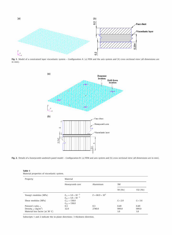
Fig. 2. Details of a honeycomb sandwich panel model – Configuration B: (a) FEM and axis system and (b) cross sectional view (all dimensions are in mm).

Table 1Material properties of viscoelastic system.

Property Material

Honeycomb core Aluminium 3M

50 (Hz) 132 (Hz)

Young's modulus (MPa) E11 ¼ 1.0�10�3 E¼ 68.9�103

E22 ¼ 1.0�10�3

Shear modulus (MPa) G13 ¼ 138.0 G¼2.0 G¼3.6G23 ¼ 138.0

Poisson's ratio, ν 0.3 0.3 0.49 0.49Density, ρ (kg/m3) 32.0 2740.0 999.0 999.0Material loss factor (at 30 1C) 1.0 1.0

Subscripts 1 and 2 indicate the in-plane directions; 3 thickness direction.

Fig. 1. Model of a constrained layer viscoelastic system – Configuration A: (a) FEM and the axis system and (b) cross sectional view (all dimensions arein mm).

K.K. Sairajan et al. / Journal of Sound and Vibration 333 (2014) 4051–4070 4055

K.K. Sairajan et al. / Journal of Sound and Vibration 333 (2014) 4051–40704056

base excitation is applied to this node in the subsequent analysis. The total mass of the system is 80.98�10�3 kg and thecoordinate system of the FEM is shown in Fig. 1a.

In Configuration B, the chosen solar panel has a rectangular shape (0.8 m�0.6 m) and the viscoelastic layers areconstrained between the two identical sandwich panels and each of these sandwich panels consists of two thinaluminium face sheets (1.0�10�4 m thick ) and a honeycomb core as shown in Fig. 2b. This configuration is chosen toobtain the maximum damping effect by placing the viscoelastic layers near the maximum shear stress area along withthe manufacturing feasibility of the sandwich assembly. The honeycomb sandwich panels are modeled using layeredshell elements (PSHELL) of Nastran and viscoelastic layers are modeled using eight nodes hexagonal elements. The solarpanel model consists of four identical hold down blocks, which support the panel to the main spacecraft during thelaunch. Each hold down has an axial stiffness of 1.0�1010 N/m and a rotational stiffness of 1.0�108 N/rad. The nodes ineach hold down area were rigidly connected together and connected to the base point using six CELAS elements, thefirst three elements correspond to the three axial stiffness and the last three correspond to the rotational stiffness. Asingle base fixed boundary condition is obtained by rigidly connecting the four base points of the hold down blocks atthe bottom of the panel.

The material properties used to model Configuration B are also given in Table 1. Here, the properties of the 3Mviscoelastic damping polymer at 30 1C and 132 Hz, that have been estimated using Ref. [28], were used in the analysis.It should be noted that 132 Hz is the average frequency of the target modes of the system as described in Section 4.1.It was also considered that the structure supports an additional mass of 2.0 kg, which accounts for solar cells, harnessetc. and this non-structural mass is uniformly distributed over the top surface of the panel. The total mass of the systemwas 3.04 kg.

3.2. Piezoelectric system

To study the correlation aspects of a piezoelectric system, a piezoelectric patch bonded onto the upper face of a titaniumplate was considered and the geometry of the configuration is shown in Fig. 3. Both the plate and piezoelectric patch have arectangular shape with a uniform thickness of 0.002 m and 3.8�10�4 m, respectively. A resistor and inductor are connectedin series between the top and the bottom electrodes of the piezoelectric patch to dissipate the vibration energy of thesystem. A similar problem has been analyzed by Min et al. [14] but here the focus is to study the correlation aspects of themulti-physics system rather than the vibration control.

Fig. 3. Details of the piezoelectric patch on the titanium plate – Configuration C (all dimensions are in mm)

The FEM of the piezoelectric system attached with a resistor (R) and inductor (L) in series is shown in Fig. 4.The piezoelectric patch is placed in such a way that it can reduce the dynamic response due to the third bending modeof the structure when it is excited by a harmonic force (fT ) at the fixed end in the Z direction as shown in Fig. 4.The modeling and the analysis were conducted using ANSYS multi-physics software. The titanium plate was modeledusing 20-node SOLID186 elements and the element has three displacement degrees of freedom per node [31].The piezoelectric patch was modeled using SOLID226 elements with the material property of PZT-5 and the resistorand inductor were modeled using CIRCU94 elements. These elements are capable of simulating the linear electriccircuits and can be directly coupled with the piezoelectric elements [32]. The properties of titanium and PZT-5used in the analysis are shown in Table 2 [14]. The poling direction for the piezoelectric material is chosen asthe thickness direction of the patch. The bonding details of the piezoelectric patch to the plate are not considered inthis analysis.

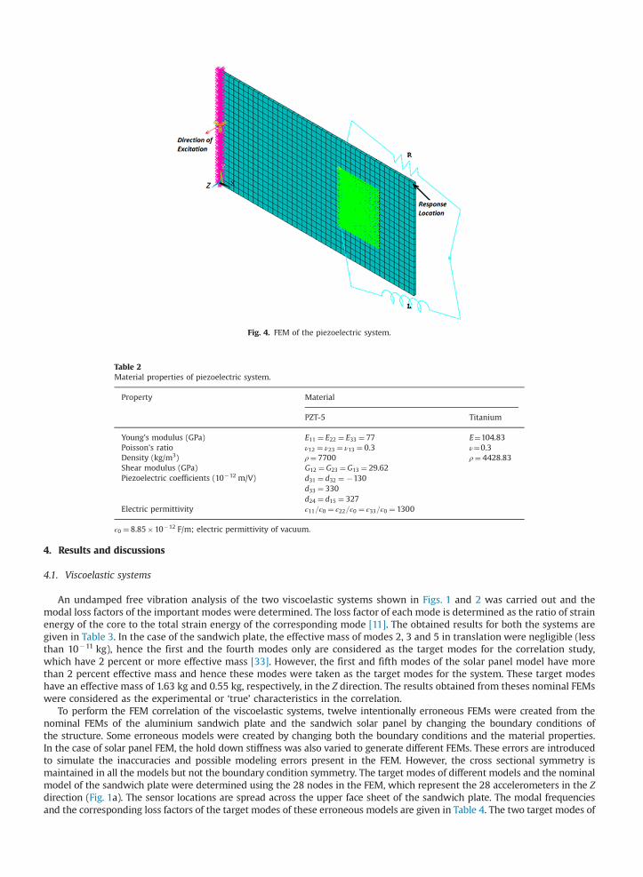
Fig. 4. FEM of the piezoelectric system.

Table 2Material properties of piezoelectric system.

Property Material

PZT-5 Titanium

Young's modulus (GPa) E11 ¼ E22 ¼ E33 ¼ 77 E¼104.83Poisson's ratio ν12 ¼ ν23 ¼ ν13 ¼ 0.3 ν¼0.3Density (kg/m3) ρ¼ 7700 ρ¼ 4428.83Shear modulus (GPa) G12 ¼ G23 ¼G13 ¼ 29.62Piezoelectric coefficients (10�12 m/V) d31 ¼ d32 ¼ �130

d33 ¼ 330d24 ¼ d15 ¼ 327

Electric permittivity ϵ11=ϵ0 ¼ ϵ22=ϵ0 ¼ ϵ33=ϵ0 ¼ 1300

ϵ0 ¼ 8.85�10�12 F/m; electric permittivity of vacuum.

K.K. Sairajan et al. / Journal of Sound and Vibration 333 (2014) 4051–4070 4057

4. Results and discussions

4.1. Viscoelastic systems

An undamped free vibration analysis of the two viscoelastic systems shown in Figs. 1 and 2 was carried out and themodal loss factors of the important modes were determined. The loss factor of each mode is determined as the ratio of strainenergy of the core to the total strain energy of the corresponding mode [11]. The obtained results for both the systems aregiven in Table 3. In the case of the sandwich plate, the effective mass of modes 2, 3 and 5 in translation were negligible (lessthan 10�11 kg), hence the first and the fourth modes only are considered as the target modes for the correlation study,which have 2 percent or more effective mass [33]. However, the first and fifth modes of the solar panel model have morethan 2 percent effective mass and hence these modes were taken as the target modes for the system. These target modeshave an effective mass of 1.63 kg and 0.55 kg, respectively, in the Z direction. The results obtained from theses nominal FEMswere considered as the experimental or ‘true’ characteristics in the correlation.

To perform the FEM correlation of the viscoelastic systems, twelve intentionally erroneous FEMs were created from thenominal FEMs of the aluminium sandwich plate and the sandwich solar panel by changing the boundary conditions ofthe structure. Some erroneous models were created by changing both the boundary conditions and the material properties.In the case of solar panel FEM, the hold down stiffness was also varied to generate different FEMs. These errors are introducedto simulate the inaccuracies and possible modeling errors present in the FEM. However, the cross sectional symmetry ismaintained in all the models but not the boundary condition symmetry. The target modes of different models and the nominalmodel of the sandwich plate were determined using the 28 nodes in the FEM, which represent the 28 accelerometers in the Zdirection (Fig. 1a). The sensor locations are spread across the upper face sheet of the sandwich plate. The modal frequenciesand the corresponding loss factors of the target modes of these erroneous models are given in Table 4. The two target modes of

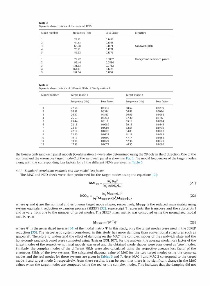
Table 4Dynamic characteristics of different FEMs of Configuration A.

Model number Target mode 1 Target mode 2

Frequency (Hz) Loss factor Frequency (Hz) Loss factor

1 27.56 0.1354 68.52 0.12032 26.91 0.1514 56.82 0.10243 26.37 0.1510 66.96 0.09664 26.53 0.1233 67.30 0.11025 25.44 0.1118 65.11 0.09046 22.12 0.0989 59.16 0.08487 23.81 0.0904 62.55 0.07388 22.18 0.0826 54.03 0.07009 22.70 0.0824 61.14 0.0683

10 19.11 0.0890 47.17 0.058311 19.94 0.0729 57.36 0.062912 17.81 0.0677 46.35 0.0606

Table 3Dynamic characteristics of the nominal FEMs.

Mode number Frequency (Hz) Loss factor Structure

1 29.13 0.14962 44.53 0.13683 68.28 0.1671 Sandwich plate4 70.21 0.12715 82.32 0.1379

1 72.22 0.0887 Honeycomb sandwich panel2 93.44 0.08843 131.53 0.07824 164.13 0.12295 191.04 0.1154

K.K. Sairajan et al. / Journal of Sound and Vibration 333 (2014) 4051–40704058

the honeycomb sandwich panel models (Configuration B) were also determined using the 28 dofs in the Z direction. One of thenominal and the erroneous target mode-2 of the sandwich panel is shown in Fig. 5. The modal frequencies of the target modesalong with the corresponding loss factors for all the different FEMs are given in Table 5.

4.1.1. Standard correlation methods and the modal loss factorThe MAC and NCO check were then performed for the target modes using the equations [2]:

MAClm ¼ jψTl ϕmj2

ðψTl ψlÞðϕT

mϕmÞ(21)

NCOlm ¼ jψTl MSEREPϕmj2

ðψTl MSEREPψlÞðϕT

mMSEREPϕmÞ(22)

where ψ and ϕ are the nominal and erroneous target mode shapes, respectively, MSEREP is the reduced mass matrix usingsystem equivalent reduction expansion process (SEREP) [32], superscript T represents the transpose and the subscripts land m vary from one to the number of target modes. The SEREP mass matrix was computed using the normalized modalmatrix, ψ, as

MSEREP ¼ ðΨ†ÞTΨ† (23)

where Ψ† is the generalized inverse [34] of the modal matrix Ψ. In this study, only the target modes were used in the SEREPreduction [35]. The viscoelastic system considered in this study has more damping than conventional structures such asspacecraft. Therefore to understand the effect of damping on the MAC, the complex modes of the sandwich plate and thehoneycomb sandwich panel were computed using Nastran (SOL 107). For the analysis, the average modal loss factor of thetarget modes of the respective nominal models was used and the obtained mode shapes were considered as ‘true’ modes.Similarly, the complex modes of the different FEMs were also calculated using the respective average loss factor of theerroneous FEMs of the two systems. The calculated diagonal value of MAC for the two target modes using the complexmodes and the real modes for these systems are given in Tables 6 and 7. Here, MAC 1 and MAC 2 correspond to the targetmode 1 and target mode 2, respectively. From these results, it can be seen that there is no significant change in the MACvalues when the target modes are computed using the real or the complex modes. This indicates that the damping did not

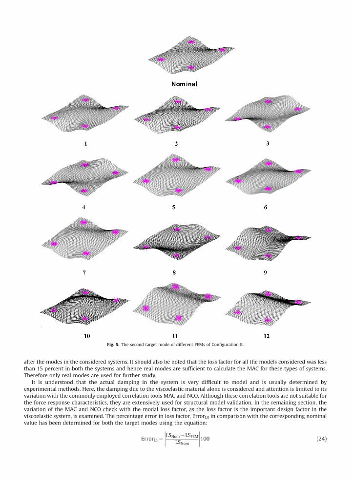
Fig. 5. The second target mode of different FEMs of Configuration B.

K.K. Sairajan et al. / Journal of Sound and Vibration 333 (2014) 4051–4070 4059

alter the modes in the considered systems. It should also be noted that the loss factor for all the models considered was lessthan 15 percent in both the systems and hence real modes are sufficient to calculate the MAC for these types of systems.Therefore only real modes are used for further study.

It is understood that the actual damping in the system is very difficult to model and is usually determined byexperimental methods. Here, the damping due to the viscoelastic material alone is considered and attention is limited to itsvariation with the commonly employed correlation tools MAC and NCO. Although these correlation tools are not suitable forthe force response characteristics, they are extensively used for structural model validation. In the remaining section, thevariation of the MAC and NCO check with the modal loss factor, as the loss factor is the important design factor in theviscoelastic system, is examined. The percentage error in loss factor, ErrorLS in comparison with the corresponding nominalvalue has been determined for both the target modes using the equation:

ErrorLS ¼�����LSNom�LSFEM

LSNom

�����100 (24)

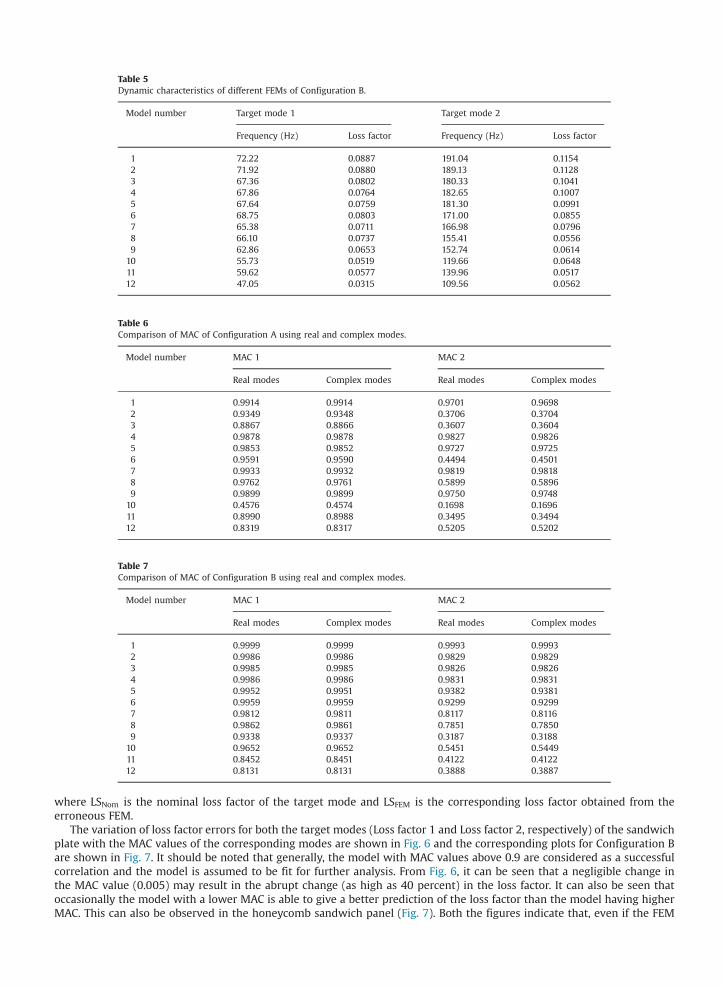
Table 5Dynamic characteristics of different FEMs of Configuration B.

Model number Target mode 1 Target mode 2

Frequency (Hz) Loss factor Frequency (Hz) Loss factor

1 72.22 0.0887 191.04 0.11542 71.92 0.0880 189.13 0.11283 67.36 0.0802 180.33 0.10414 67.86 0.0764 182.65 0.10075 67.64 0.0759 181.30 0.09916 68.75 0.0803 171.00 0.08557 65.38 0.0711 166.98 0.07968 66.10 0.0737 155.41 0.05569 62.86 0.0653 152.74 0.0614

10 55.73 0.0519 119.66 0.064811 59.62 0.0577 139.96 0.051712 47.05 0.0315 109.56 0.0562

Table 7Comparison of MAC of Configuration B using real and complex modes.

Model number MAC 1 MAC 2

Real modes Complex modes Real modes Complex modes

1 0.9999 0.9999 0.9993 0.99932 0.9986 0.9986 0.9829 0.98293 0.9985 0.9985 0.9826 0.98264 0.9986 0.9986 0.9831 0.98315 0.9952 0.9951 0.9382 0.93816 0.9959 0.9959 0.9299 0.92997 0.9812 0.9811 0.8117 0.81168 0.9862 0.9861 0.7851 0.78509 0.9338 0.9337 0.3187 0.3188

10 0.9652 0.9652 0.5451 0.544911 0.8452 0.8451 0.4122 0.412212 0.8131 0.8131 0.3888 0.3887

Table 6Comparison of MAC of Configuration A using real and complex modes.

Model number MAC 1 MAC 2

Real modes Complex modes Real modes Complex modes

1 0.9914 0.9914 0.9701 0.96982 0.9349 0.9348 0.3706 0.37043 0.8867 0.8866 0.3607 0.36044 0.9878 0.9878 0.9827 0.98265 0.9853 0.9852 0.9727 0.97256 0.9591 0.9590 0.4494 0.45017 0.9933 0.9932 0.9819 0.98188 0.9762 0.9761 0.5899 0.58969 0.9899 0.9899 0.9750 0.9748

10 0.4576 0.4574 0.1698 0.169611 0.8990 0.8988 0.3495 0.349412 0.8319 0.8317 0.5205 0.5202

K.K. Sairajan et al. / Journal of Sound and Vibration 333 (2014) 4051–40704060

where LSNom is the nominal loss factor of the target mode and LSFEM is the corresponding loss factor obtained from theerroneous FEM.

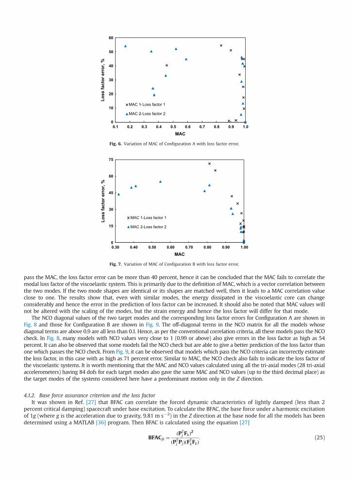
The variation of loss factor errors for both the target modes (Loss factor 1 and Loss factor 2, respectively) of the sandwichplate with the MAC values of the corresponding modes are shown in Fig. 6 and the corresponding plots for Configuration Bare shown in Fig. 7. It should be noted that generally, the model with MAC values above 0.9 are considered as a successfulcorrelation and the model is assumed to be fit for further analysis. From Fig. 6, it can be seen that a negligible change inthe MAC value (0.005) may result in the abrupt change (as high as 40 percent) in the loss factor. It can also be seen thatoccasionally the model with a lower MAC is able to give a better prediction of the loss factor than the model having higherMAC. This can also be observed in the honeycomb sandwich panel (Fig. 7). Both the figures indicate that, even if the FEM

0

10

20

30

40

50

60

0.1 0.2 0.3 0.4 0.5 0.6 0.7 0.8 0.9 1.0

Loss

fact

or e

rror

, %

MAC

MAC 1 - Loss factor 1

MAC 2 - Loss factor 2

Fig. 6. Variation of MAC of Configuration A with loss factor error.

0

15

30

45

60

75

0.30 0.40 0.50 0.60 0.70 0.80 0.90 1.00

Loss

fact

or e

rror

, %

MAC

MAC 1-Loss factor 1

MAC 2-Loss factor 2

Fig. 7. Variation of MAC of Configuration B with loss factor error.

K.K. Sairajan et al. / Journal of Sound and Vibration 333 (2014) 4051–4070 4061

pass the MAC, the loss factor error can be more than 40 percent, hence it can be concluded that the MAC fails to correlate themodal loss factor of the viscoelastic system. This is primarily due to the definition of MAC, which is a vector correlation betweenthe two modes. If the two mode shapes are identical or its shapes are matched well, then it leads to a MAC correlation valueclose to one. The results show that, even with similar modes, the energy dissipated in the viscoelastic core can changeconsiderably and hence the error in the prediction of loss factor can be increased. It should also be noted that MAC values willnot be altered with the scaling of the modes, but the strain energy and hence the loss factor will differ for that mode.

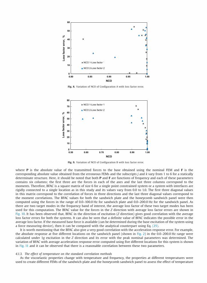
The NCO diagonal values of the two target modes and the corresponding loss factor errors for Configuration A are shown inFig. 8 and those for Configuration B are shown in Fig. 9. The off-diagonal terms in the NCO matrix for all the models whosediagonal terms are above 0.9 are all less than 0.1. Hence, as per the conventional correlation criteria, all these models pass the NCOcheck. In Fig. 8, many models with NCO values very close to 1 (0.99 or above) also give errors in the loss factor as high as 54percent. It can also be observed that some models fail the NCO check but are able to give a better prediction of the loss factor thanone which passes the NCO check. From Fig. 9, it can be observed that models which pass the NCO criteria can incorrectly estimatethe loss factor, in this case with as high as 71 percent error. Similar to MAC, the NCO check also fails to indicate the loss factor ofthe viscoelastic systems. It is worth mentioning that the MAC and NCO values calculated using all the tri-axial modes (28 tri-axialaccelerometers) having 84 dofs for each target modes also gave the same MAC and NCO values (up to the third decimal place) asthe target modes of the systems considered here have a predominant motion only in the Z direction.

4.1.2. Base force assurance criterion and the loss factorIt was shown in Ref. [27] that BFAC can correlate the forced dynamic characteristics of lightly damped (less than 2

percent critical damping) spacecraft under base excitation. To calculate the BFAC, the base force under a harmonic excitationof 1g (where g is the acceleration due to gravity, 9.81 m s�2) in the Z direction at the base node for all the models has beendetermined using a MATLAB [36] program. Then BFAC is calculated using the equation [27]

BFACjk ¼ðPT

j FkÞ2

ðPTj PjÞðFTkFkÞ

: (25)

0

10

20

30

40

50

60

0.80 0.85 0.90 0.95 1.00

Loss

fact

or e

rror

, %

NCO

NCO 1-Loss factor 1

NCO 2-Loss factor 2

Fig. 8. Variation of NCO of Configuration A with loss factor error.

0

10

20

30

40

50

60

70

80

0.50 0.60 0.70 0.80 0.90 1.00

Loss

fact

or e

rror

, %

NCO

NCO 1-Loss factor 1

NCO 2-Loss factor 2

Fig. 9. Variation of NCO of Configuration B with loss factor error.

K.K. Sairajan et al. / Journal of Sound and Vibration 333 (2014) 4051–40704062

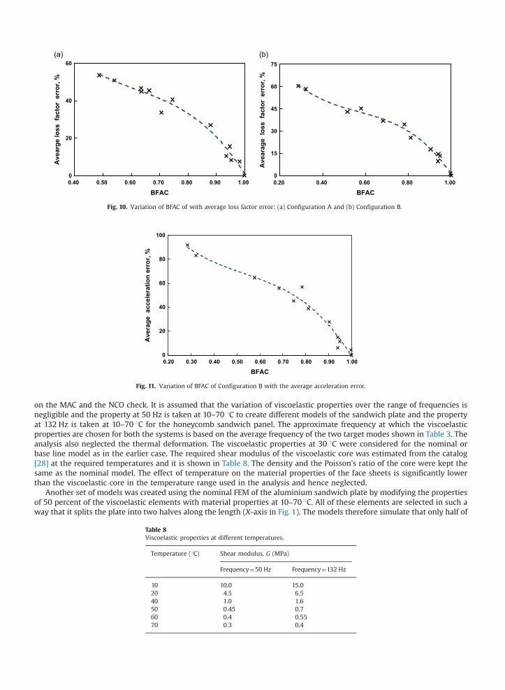
where P is the absolute value of the transmitted forces to the base obtained using the nominal FEM and F is thecorresponding absolute value obtained from the erroneous FEMs and the subscripts j and k vary from 1 to 6 for a staticallydeterminate structure. Here, it should be noted that both P and F are functions of frequency and each of these parameterscontains six columns; the first three are the forces in each of the axes and the last three columns correspond to themoments. Therefore, BFAC is a square matrix of size 6 for a single point constrained system or a system with interfaces arerigidly connected to a single location as in this study and its values vary from 0.0 to 1.0. The first three diagonal valuesin this matrix correspond to the correlation of forces in three directions and the last three diagonal values correspond tothe moment correlations. The BFAC values for both the sandwich plate and the honeycomb sandwich panel were thencomputed using the forces in the range of 0.0–100.0 Hz for sandwich plate and 0.0–200.0 Hz for the sandwich panel. Asthere are two target modes in the frequency band of interest, the average loss factor of these two target modes has beenused for this computation. The BFAC value for the forces in the Z direction with average loss factor errors are shown inFig. 10. It has been observed that, BFAC in the direction of excitation (Z direction) gives good correlation with the averageloss factor errors for both the systems. It can also be seen that a definite value of BFAC indicates the possible error in theaverage loss factor. If the measured base force is available (can be determined during the base excitation of the system usinga force measuring device), then it can be compared with the analytical counterpart using Eq. (25).

It is worth mentioning that the BFAC also give a very good correlation with the acceleration response error. For example,the absolute response at five different locations on the sandwich panel (shown in Fig. 2) in the 0.0–200.0 Hz range werecalculated under 1g excitation in the Z direction and its error with the peak nominal parameters was determined. Thevariation of BFAC with average acceleration response error computed using five different locations for this system is shownin Fig. 11 and it can be observed that there is a reasonable correlation between these two parameters.

4.1.3. The effect of temperature on the standard correlation methodsAs the viscoelastic properties change with temperature and frequency, the properties at different temperatures were

used to create different FEMs of the sandwich plate and the honeycomb sandwich panel to assess the effect of temperature

0

20

40

60

0.40 0.50 0.60 0.70 0.80 0.90 1.00

Ave

arge

loss

fac

tor

erro

r, %

BFAC

0

15

30

45

60

75

0.20 0.40 0.60 0.80 1.00

Ave

arag

e lo

ss f

acto

r er

ror,

%

BFAC

Fig. 10. Variation of BFAC of with average loss factor error: (a) Configuration A and (b) Configuration B.

0

20

40

60

80

100

0.20 0.30 0.40 0.50 0.60 0.70 0.80 0.90 1.00

Ave

rage

acc

eler

atio

n er

ror,

%

BFAC

Fig. 11. Variation of BFAC of Configuration B with the average acceleration error.

K.K. Sairajan et al. / Journal of Sound and Vibration 333 (2014) 4051–4070 4063

on the MAC and the NCO check. It is assumed that the variation of viscoelastic properties over the range of frequencies isnegligible and the property at 50 Hz is taken at 10–70 1C to create different models of the sandwich plate and the propertyat 132 Hz is taken at 10–70 1C for the honeycomb sandwich panel. The approximate frequency at which the viscoelasticproperties are chosen for both the systems is based on the average frequency of the two target modes shown in Table 3. Theanalysis also neglected the thermal deformation. The viscoelastic properties at 30 1C were considered for the nominal orbase line model as in the earlier case. The required shear modulus of the viscoelastic core was estimated from the catalog[28] at the required temperatures and it is shown in Table 8. The density and the Poisson's ratio of the core were kept thesame as the nominal model. The effect of temperature on the material properties of the face sheets is significantly lowerthan the viscoelastic core in the temperature range used in the analysis and hence neglected.

Another set of models was created using the nominal FEM of the aluminium sandwich plate by modifying the propertiesof 50 percent of the viscoelastic elements with material properties at 10–70 1C. All of these elements are selected in such away that it splits the plate into two halves along the length (X-axis in Fig. 1). The models therefore simulate that only half of

Table 8Viscoelastic properties at different temperatures.

Temperature (1C) Shear modulus, G (MPa)

Frequency¼50 Hz Frequency¼132 Hz

10 10.0 15.020 4.5 6.540 1.0 1.650 0.45 0.760 0.4 0.5570 0.3 0.4

K.K. Sairajan et al. / Journal of Sound and Vibration 333 (2014) 4051–40704064

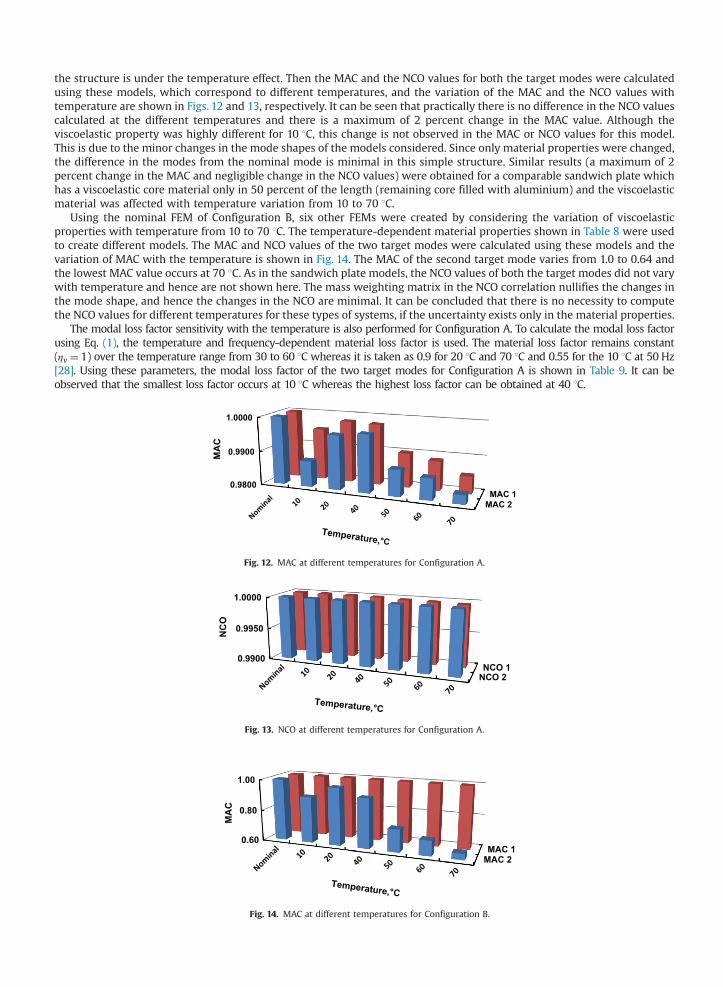
the structure is under the temperature effect. Then the MAC and the NCO values for both the target modes were calculatedusing these models, which correspond to different temperatures, and the variation of the MAC and the NCO values withtemperature are shown in Figs. 12 and 13, respectively. It can be seen that practically there is no difference in the NCO valuescalculated at the different temperatures and there is a maximum of 2 percent change in the MAC value. Although theviscoelastic property was highly different for 10 1C, this change is not observed in the MAC or NCO values for this model.This is due to the minor changes in the mode shapes of the models considered. Since only material properties were changed,the difference in the modes from the nominal mode is minimal in this simple structure. Similar results (a maximum of 2percent change in the MAC and negligible change in the NCO values) were obtained for a comparable sandwich plate whichhas a viscoelastic core material only in 50 percent of the length (remaining core filled with aluminium) and the viscoelasticmaterial was affected with temperature variation from 10 to 70 1C.

Using the nominal FEM of Configuration B, six other FEMs were created by considering the variation of viscoelasticproperties with temperature from 10 to 70 1C. The temperature-dependent material properties shown in Table 8 were usedto create different models. The MAC and NCO values of the two target modes were calculated using these models and thevariation of MAC with the temperature is shown in Fig. 14. The MAC of the second target mode varies from 1.0 to 0.64 andthe lowest MAC value occurs at 70 1C. As in the sandwich plate models, the NCO values of both the target modes did not varywith temperature and hence are not shown here. The mass weighting matrix in the NCO correlation nullifies the changes inthe mode shape, and hence the changes in the NCO are minimal. It can be concluded that there is no necessity to computethe NCO values for different temperatures for these types of systems, if the uncertainty exists only in the material properties.

The modal loss factor sensitivity with the temperature is also performed for Configuration A. To calculate the modal loss factorusing Eq. (1), the temperature and frequency-dependent material loss factor is used. The material loss factor remains constant(ηv ¼ 1) over the temperature range from 30 to 60 1C whereas it is taken as 0.9 for 20 1C and 70 1C and 0.55 for the 10 1C at 50 Hz[28]. Using these parameters, the modal loss factor of the two target modes for Configuration A is shown in Table 9. It can beobserved that the smallest loss factor occurs at 10 1C whereas the highest loss factor can be obtained at 40 1C.

MAC 2MAC 1

0.9800

0.9900

1.0000

MA

C

Temperature,°C

Fig. 12. MAC at different temperatures for Configuration A.

NCO 2NCO 1

0.9900

0.9950

1.0000

NC

O

Temperature,°C

Fig. 13. NCO at different temperatures for Configuration A.

MAC 2MAC 1

0.60

0.80

1.00

MA

C

Temperature,°C

Fig. 14. MAC at different temperatures for Configuration B.

Table 9Variation of modal loss factor with temperature.

Temperature (1C) Modal loss factor

Target mode 1 Target mode 2

30 (Nominal) 0.1496 0.127110 0.0296 0.040520 0.0872 0.098240 0.1779 0.117650 0.1651 0.087860 0.1593 0.082870 0.1282 0.0635

K.K. Sairajan et al. / Journal of Sound and Vibration 333 (2014) 4051–4070 4065

4.2. Piezoelectric system

4.2.1. Dynamic responseThe piezoelectric system shown previously in Fig. 4 has been analyzed under the 0.1g base excitation in the Z direction

without any electrical circuits and the bottom electrode of the piezoelectric patch, which interfaces with the plate, in agrounded condition. The critical damping ratio was taken as 7.8�10�4 [14] and the absolute acceleration response at the tipof the cantilever during the third bending mode is shown in Fig. 15. This response has peak amplitude of 27.43g and occursat 724.6 Hz. Then the piezoelectric electrodes are attached with a resistance (1 Ω) and an inductor (0.65 H). The dynamicresponse at the tip with these electrical components is also shown in Fig. 15. The first peak in this figure is the electricalresonance that occurs at 639.7 Hz. These typical values of the electrical parameters are chosen to show a distinct electricalresonance mode. It can be observed that there is a slight decrease in the tip acceleration (7.6 percent) during the thirdbending mode compared to the system which does not have any electrical circuits. If further reduction in the peakacceleration response is required, the electrical circuit parameters can be tuned. One such option with R¼1000 Ω andL¼0.65 H gives a tip acceleration as low as 4.4g during the third bending mode for the same base excitation and thisresponse plot is also shown in Fig. 15.

4.2.2. Correlation of finite element model of a piezoelectric systemTo understand how the FEM of a piezoelectric system performs under dynamic loading when it possesses a certain value

of the MAC, a study has been carried out using the different FEMs generated from the nominal FEM. It is understood that theMAC is not a criterion for the response analysis but it is the most popular correlation method. The FEM generated using thematerial property shown in Table 2 is considered as the nominal model and the obtained results were taken as theexperimental or ‘true’ results for the correlation study. It is understood that there is a good amount of uncertainty inthe properties of piezoelectric material [13,14], and hence ten different intentionally erroneous FEMs were generated fromthe nominal FEM by varying all the material properties of the system from 0.5 to 25.0 percent of the nominal value shown inTable 2. The percentage increase in the material properties for different erroneous models was chosen as 0.5, 0.75, 1.0, 2.5,5.0, 7.5, 10.0, 15.0, 20.0, and 25.0. Geometry, boundary condition and the electrical shunt circuit (R¼1 Ω, L¼0.65 H) werekept constant throughout.

Tip acceleration, tip displacement and the peak current in the electrical circuit were computed in the frequency range of5.0–750.0 Hz during the base excitation of the system. As in the previous case, the input acceleration was 0.1g in the Zdirection. The percentage error in the absolute acceleration, the absolute tip displacement for the third bending mode and

0

5

10

15

20

25

30

600 625 650 675 700 725 750

Acc

eler

atio

n, g

Frequency, Hz

Without R and L

R=1.0 Ohm, L= 0.65 H

R=1000.0 Ohm, L=0.65 H

Electrical Resonance

Fig. 15. Tip acceleration with different configurations the of electrical circuit.

K.K. Sairajan et al. / Journal of Sound and Vibration 333 (2014) 4051–40704066

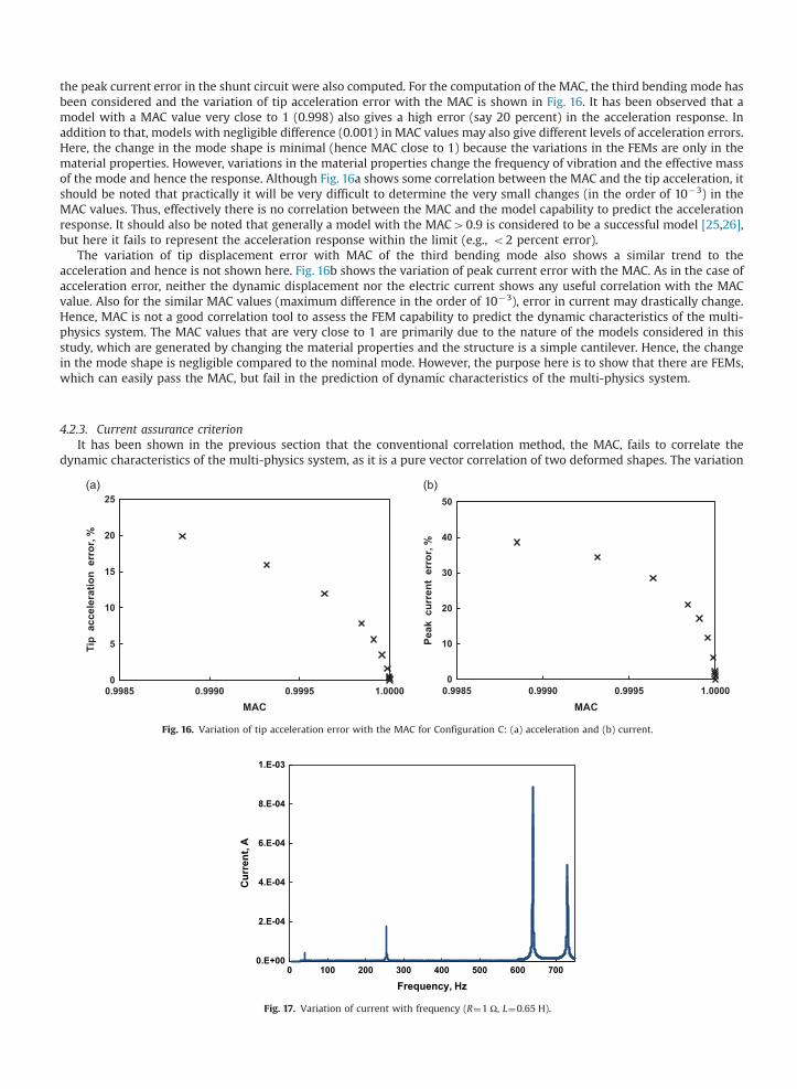
the peak current error in the shunt circuit were also computed. For the computation of the MAC, the third bending mode hasbeen considered and the variation of tip acceleration error with the MAC is shown in Fig. 16. It has been observed that amodel with a MAC value very close to 1 (0.998) also gives a high error (say 20 percent) in the acceleration response. Inaddition to that, models with negligible difference (0.001) in MAC values may also give different levels of acceleration errors.Here, the change in the mode shape is minimal (hence MAC close to 1) because the variations in the FEMs are only in thematerial properties. However, variations in the material properties change the frequency of vibration and the effective massof the mode and hence the response. Although Fig. 16a shows some correlation between the MAC and the tip acceleration, itshould be noted that practically it will be very difficult to determine the very small changes (in the order of 10�3) in theMAC values. Thus, effectively there is no correlation between the MAC and the model capability to predict the accelerationresponse. It should also be noted that generally a model with the MAC40.9 is considered to be a successful model [25,26],but here it fails to represent the acceleration response within the limit (e.g., o2 percent error).

The variation of tip displacement error with MAC of the third bending mode also shows a similar trend to theacceleration and hence is not shown here. Fig. 16b shows the variation of peak current error with the MAC. As in the case ofacceleration error, neither the dynamic displacement nor the electric current shows any useful correlation with the MACvalue. Also for the similar MAC values (maximum difference in the order of 10�3), error in current may drastically change.Hence, MAC is not a good correlation tool to assess the FEM capability to predict the dynamic characteristics of the multi-physics system. The MAC values that are very close to 1 are primarily due to the nature of the models considered in thisstudy, which are generated by changing the material properties and the structure is a simple cantilever. Hence, the changein the mode shape is negligible compared to the nominal mode. However, the purpose here is to show that there are FEMs,which can easily pass the MAC, but fail in the prediction of dynamic characteristics of the multi-physics system.

4.2.3. Current assurance criterionIt has been shown in the previous section that the conventional correlation method, the MAC, fails to correlate the

dynamic characteristics of the multi-physics system, as it is a pure vector correlation of two deformed shapes. The variation

0

5

10

15

20

25

0.9985 0.9990 0.9995 1.0000

Tip

acc

eler

atio

n e

rror

, %

MAC

0

10

20

30

40

50

0.9985 0.9990 0.9995 1.0000

Peak

cur

rent

err

or, %

MAC

Fig. 16. Variation of tip acceleration error with the MAC for Configuration C: (a) acceleration and (b) current.

0.E+00

2.E-04

4.E-04

6.E-04

8.E-04

1.E-03

0 100 200 300 400 500 600 700

Cur

rent

, A

Frequency, Hz

Fig. 17. Variation of current with frequency (R¼1 Ω, L¼0.65 H).

K.K. Sairajan et al. / Journal of Sound and Vibration 333 (2014) 4051–4070 4067

of the nominal value of the current with frequency, when the piezoelectric structure is connected with the electric circuit isexcited with a harmonic input (0.1g) at the base is shown in Fig. 17. The maximum current in the circuit occurs during theelectrical resonance and in this chosen configuration it occurs at 639.7 Hz. The other three peaks in the figure correspond tothe first three bending modes of the structure, which occur at 39.4 Hz, 255.1 Hz, and 730.8 Hz, respectively. It can be notedthat, unlike acceleration or displacement, current in the shunt circuit does not depend on the location and will be unique foreach circuit. However, current in the circuit varies with the frequency and the current values in the frequency range containimportant information about the dynamics of the system. Using this property, in line with the base force assurance criterion,a current assurance criterion is defined as

CAC¼ ðITExpIFEMÞ2

ðITExpIExpÞðITFEMIFEMÞ(26)

where IExp and IFEM are the experimental and the analytically calculated absolute current values in the electrical circuit. Itshould be noted that both of these quantities are functions of frequency and all the values of current in the frequencydomain of interest need to be included for the CAC computation. This quality indicator varies from 0.0 to 1.0 where 1.0indicates a perfect correlation between the experimental and the analytical result. If there are a number of piezoelectricpatches connected with separate electrical networks or there are a series of shunt circuits, then for such different currentvalues, separate CAC need to be evaluated for the purpose of correlation. During dynamic testing, the value of the currentcan be measured for the frequency range of interest.

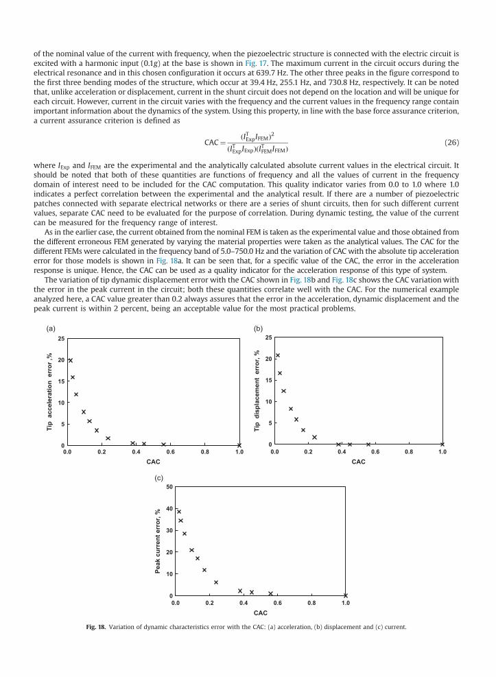
As in the earlier case, the current obtained from the nominal FEM is taken as the experimental value and those obtained fromthe different erroneous FEM generated by varying the material properties were taken as the analytical values. The CAC for thedifferent FEMs were calculated in the frequency band of 5.0–750.0 Hz and the variation of CAC with the absolute tip accelerationerror for those models is shown in Fig. 18a. It can be seen that, for a specific value of the CAC, the error in the accelerationresponse is unique. Hence, the CAC can be used as a quality indicator for the acceleration response of this type of system.

The variation of tip dynamic displacement error with the CAC shown in Fig. 18b and Fig. 18c shows the CAC variationwiththe error in the peak current in the circuit; both these quantities correlate well with the CAC. For the numerical exampleanalyzed here, a CAC value greater than 0.2 always assures that the error in the acceleration, dynamic displacement and thepeak current is within 2 percent, being an acceptable value for the most practical problems.

0

5

10

15

20

25

0.0 0.2 0.4 0.6 0.8 1.0

Tip

acc

eler

atio

n e

rror

,%

CAC

0

5

10

15

20

25

0.0 0.2 0.4 0.6 0.8 1.0

Tip

dis

plac

emen

t er

ror,

%

CAC

0

10

20

30

40

50

0.0 0.2 0.4 0.6 0.8 1.0

Peak

cur

rent

err

or, %

CAC

Fig. 18. Variation of dynamic characteristics error with the CAC: (a) acceleration, (b) displacement and (c) current.

K.K. Sairajan et al. / Journal of Sound and Vibration 333 (2014) 4051–40704068

5. Conclusion

Viscoelastic materials and electric circuit-fed piezoelectric systems have been used for vibration reduction and thecorrelation of FEMs of such systems has been studied in this work. The effectiveness of the MAC and NCO check on theprediction of the modal loss factor for two subsystems has been analyzed using intentionally erroneous FEMs. To assessthe effect of damping on the MAC, the MAC was computed using the complex modes and it was observed that there is nosignificant change compared to the corresponding value determined from the real modes. Hence, only real modes were usedfor further analysis and observed that these correlation methods do not give any indication on the capability of the model topredict the loss factor. The recently introduced BFAC is found to be more effective than the MAC or NCO check in theprediction of loss factor of such systems. Also, the effect of temperature on the MAC and NCO check were studied and notedthat there is a change in the MAC values with temperature. However, the NCO values do not vary within the temperatureband considered (10–70 1C) for both systems. This indicates that the FEM does not need to be correlated at differenttemperatures using the NCO criterion if the uncertainty is mainly attributed to the material properties of the systemsconsidered.

In addition, the FEM of a structure attached with an electric circuit-fed piezoelectric material has been reviewed. Thismulti-physics system consists of a cantilever plate, a piezoelectric patch on the top of the plate and a RL circuit in series.The FEM correlation of the coupled system is carried out using the nominal FEM and the intentionally erroneous models andobserved that MAC does not display any useful correlation to the dynamic characteristics. This is because even if there is noobservable change in the mode shapes as in this cantilever structure, the response of the structure still varies. However, asthe MAC is based on mode shape correlation it will still indicate a high value. A new correlation tool identified as the CAC isintroduced by comparing the electric current in the circuit during the harmonic excitation obtained from the nominalmodel, and that noted from the erroneous FEM. A good correlation has been obtained between the CAC and the structuraldynamic characteristics error and the error in the peak current. For the typical problem considered in this study, a CAC valueof 0.2 always assures that the error in the response is within 2 percent, hence the CAC can be used for the assessment ofFEMs of these types of multi-physics systems.

Acknowledgments

The authors wish to acknowledge the Commonwealth Scholarship Commission, UK (No. INCS-2010-188), for theirfunding. They would also like to thank Thomas K. Joseph, Scientist – ISRO Satellite Centre, Bangalore for the help in Nastransoftware.

Appendix A. An approximate expression for the modal loss factor

The modal loss factor of the complex structure with viscoelastic damping was calculated using the approximate methodproposed by Johnson and Kienholz [11]. This approach is based on the modal strain energy method introduced by Ungar [9]and the derivation for the modal loss factor using this method is given below [11].

The equation for the free vibration of viscoelastic system can be written as

M €xþðKReþ iKImÞx¼ 0 (A.1)

>where KRe and KIm are the real and the imaginary part of the stiffness matrix. The equation can be converted to aneigenvalue problem by considering a solution,

x¼ ϕreiλr t (A.2)

where λr and ϕ are the rth complex eigenvalue and eigenvector. The complex eigenvalue can also be written as

λr ¼ λrffiffiffiffiffiffiffiffiffiffiffiffiffi1þ iηr

p(A.3)

where ηr represents the loss factor of the rth mode. For the complex stiffness matrix considered in Eq. (A.1), the Raleigh'squotient formula can be written after dropping the mode index r as

λ2 ¼ λ2þ iηλ2 ¼ ϕTKReϕ

ϕTMϕþ i

ϕTKImϕϕTMϕ

: (A.4)

The loss factor can be approximated by replacing the complex eigenvector ϕ with the real eigenvector, ϕ in Eq. (A.4). Inthis case, the real eigenvector can be obtained by neglecting the imaginary part of the stiffness matrix and solving the pure

K.K. Sairajan et al. / Journal of Sound and Vibration 333 (2014) 4051–4070 4069

elastic eigenvalue problem. Then, equating the real and imaginary parts gives

λ2 ¼ ϕTKReϕϕTMϕ

(A.5)

ηλ2 ¼ ϕTKImϕϕTMϕ

: (A.6)

The stiffness matrix obtained using the finite element analysis can be segregated to the terms corresponding tothe elastic elements, Ke and the viscoelastic elements, Kv. The second matrix will be a complex matrix, but for a singleviscoelastic material, its imaginary part ðKvIÞ and real part ðKvRÞ follow the relation:

KvI ¼ ηvKvR (A.7)

where ηv is the loss factor of the viscoelastic material at the rth resonant frequency. Hence,

Kv ¼KvRþ iKvI ¼KvRð1þ iηvÞ: (A.8)

Assuming that only the complex part of Kv contributes to the imaginary part of the system stiffness matrix, then

KIm ¼KvI : (A.9)

Let VT be the total strain energy obtained when a purely elastic normal mode analysis is performed. This can becalculated using the normal mode as

VT ¼ ϕTKReϕ: (A.10)

A portion of the total strain energy will be contributed by the viscoelastic elements and it is given by

Vv ¼ ϕTKvRϕ: (A.11)

Using Eqs. (A.5) and (A.6), the modal loss factor can be obtained as

η¼ ϕTKImϕϕTKReϕ

: (A.12)

Using the relationship shown in Eqs. (A.9) and (A.7), the above equation can be re-written as

η¼ ηvϕTKvRϕϕTKReϕ

: (A.13)

Substituting Eqs. (A.10) and (A.11) in Eq. (A.13) and reintroducing mode superscript r gives the loss factor as

ηr ¼ ηvVrv

VrT

� �: (A.14)

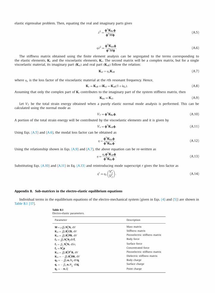
Appendix B. Sub-matrices in the electro-elastic equilibrium equations

Individual terms in the equilibrium equations of the electro-mechanical system (given in Eqs. (4) and (5)) are shown inTable B.1 [17].

Table B.1Electro-elastic parameters.

Parameter Description

M¼ ρ∭VNTxNx dV Mass matrix

Kxx ¼∭VBTxCBx dV Stiffness matrix

Kxv ¼∭VBTxPBv dV Piezoelectric stiffness matrix

fB ¼∭VNTxNf dVf i

Body force

fS ¼∬S1NTxNs dSsi Surface force

fp ¼NTxp Concentrated force

Kvx ¼∭VBTvP

TBx dV Piezoelectric stiffness matrix

Kvv ¼ �∭VBTvDBv dV Dielectric stiffness matrix

qB ¼ �∭VnvNq dVqi Body charge

qs ¼ �∬S2nvNq0 dSq

0i

Surface charge

qp ¼ �nvQ Point charge

K.K. Sairajan et al. / Journal of Sound and Vibration 333 (2014) 4051–40704070

References

[1] R.M. Lin, J. Zhu, Finite element model updating using vibration test data under base excitation, Journal of Sound and Vibration 303 (2007) 596–613,http://dx.doi.org/10.1016/j.jsv.2007.01.029.

[2] R.J. Allemang, D.L. Brown, A correlation coefficient for modal vector analysis, Proceedings of First International Modal Analysis Conference, Society forExperimental Mechanics, Connecticut, USA, 1982, pp. 110–116.

[3] D.J. Ewins, Modal Testing Theory, Practice and Application, Engineering Dynamics Series, 2nd ed. Research Studies Press Ltd., Baldock, England, 2000.[4] N.A.J. Lieven, D.J. Ewins, Spatial correlation of mode shapes: the coordinate modal assurance criterion (COMAC), Proceedings of Sixth International

Modal Analysis Conference, Society for Experimental Mechanics, Connecticut, USA, 1988, pp. 690–695.[5] D. Nefske, S. Sung, Correlation of a coarse mesh finite element model using structural system identification and a frequency response criterion,

Proceedings of 14th International Model Analysis Conference, Society for Experimental Mechanics, Connecticut, USA, 1996, pp. 597–602.[6] R.A.S. Moreira, J.D. Rodrigues, Multilayer damping treatments: modeling and experimental assessment, Journal of Sandwich Structures and Materials 12

(2010) 181–198, http://dx.doi.org/10.1177/1099636209104530.[7] M.D. Rao, Recent applications of viscoelastic damping for noise control in automobiles and commercial airplanes, Journal of Sound and Vibration 262

(2003) 457–474, http://dx.doi.org/10.1016/s0022-460x(03)00106-8.[8] D.J. Mead, Passive Vibration Control, John Wiley & Sons Ltd., West Sussex, England, 2000.[9] E.E. Ungar, E.M. Kerwin, Loss factors of viscoelastic systems in terms of energy concepts, The Journal of the Acoustical Society of America 34 (1962)

954–957.[10] C.T. Sun, B.V. Sankar, V.S. Rao, Damping and vibration control of unidirectional composite laminates using add-on viscoelastic materials, Journal of

Sound and Vibration 139 (1990) 277–287, http://dx.doi.org/10.1016/0022-460x(90)90888-7.[11] C.D. Johnson, D.A. Kienholz, Finite-element prediction of damping in structures with constrained viscoelastic layers, AIAA Journal 20 (1982) 1284–1290,

http://dx.doi.org/10.2514/3.51190.[12] P. Bangarubabu, K. Kishore Kumar, Y. Krishna, Damping effect of viscoelastic materials on sandwich beams, International Conference on Trends in

Industrial and Mechanical Engineering, Planetary Scientific Research Centre, Dubai, 2012.[13] J. Becker, O. Fein, M. Maess, L. Gaul, Finite element-based analysis of shunted piezoelectric structures for vibration damping, Computers and Structures

84 (2006) 2340–2350, http://dx.doi.org/10.1016/j.compstruc.2006.08.067.[14] J.B. Min, K.P. Duffy, A.J. Provenza, Shunted piezoelectric vibration damping analysis including centrifugal loading effects, 51st AIAA/ASME/ASCE/AHS/ASC

Structures, Structural Dynamics, and Materials Conference, Orlando, Florida, AIAA 2010-2716, 2010.[15] G. Caruso, A critical analysis of electric shunt circuits employed in piezoelectric passive vibration damping, Smart Materials and Structures 10 (2001)

1059–1068, http://dx.doi.org/10.1088/0964-1726/10/5/322.[16] E.P. Eernisse, Variational method for electroelastic vibration analysis, IEEE Transactions on Sonics and Ultrasonics 14 (1967) 153–160.[17] H. Allik, T.J.R. Hughes, Finite element method for piezoelectric vibration, International Journal for Numerical Methods in Engineering 2 (1970) 151–157,

http://dx.doi.org/10.1002/nme.1620020202.[18] P. Cupial, Three-dimensional natural vibration analysis and energy considerations for a piezoelectric rectangular plate, Journal of Sound and Vibration

283 (2005) 1093–1113, http://dx.doi.org/10.1016/j.jsv.2004.06.019.[19] H.S. Tzou, R. Ye, Piezothermoelasticity and precision control of piezoelectric systems – theory and finite-element analysis, Journal of Vibration and

Acoustics-Transactions of the ASME 116 (1994) 489–495, http://dx.doi.org/10.1115/1.2930454.[20] J.S. Wang, D.F. Ostergaard, A finite element-electric circuit coupled simulation method for piezoelectric transducer, Proceedings of IEEE Ultrasonics

Symposium, IEEE, Washington, 1999, pp. 1105–1108.[21] M.C. Reaves, L.G. Horta, Piezoelectric Actuator Modeling Using Msc/Nastran and Matlab, NASA/TM-2003-212651, Langley Research Center, 2003.[22] M.W. Al-Hazmi, Finite element analysis of cantilever plate structure excited by patches of piezoelectric actuators, Proceedings of 11th IEEE Intersociety

Conference on Thermal and Thermomechanical Phenomena in Electronic Systems 1–3, IEEE, USA, 2008, pp. 809–814.[23] B. Seba, J. Ni, B. Lohmann, Vibration attenuation using a piezoelectric shunt circuit based on finite element method analysis, Smart Materials and

Structures 15 (2006) 509–517, http://dx.doi.org/10.1088/0964-1726/15/2/034.[24] Ansys Multiphysics, 14.0 ed, ANSYS, Inc., Canonsburg, Pennsylvania, 2011.[25] Loads Analysis of Spacecraft and Payloads, NASA-STD-5002, URL: ⟨https://standards.nasa.gov/training/nasa-std-5002/index.html⟩ (accessed 23.03.11).[26] Modal Survey Assessment, ECSS-E-ST-32-11C, European Space Agency, 2008, p. 49.[27] K.K. Sairajan, G.S. Aglietti, Study of the correlation criteria for base excitation of spacecraft structures, Journal of Spacecraft and Rockets 51 (2014)

106–116, http://dx.doi.org/10.2514/1.A32457.[28] 3M™ Ultra-Pure Viscoelastic Damping Polymer, Electronics Markets Materials Division, 3M Center, St. Paul, Minnesota, Mar., 2012. URL: ⟨http://

multimedia.3m.com/mws/mediawebserver?mwsId=66666UF6EVsSyXTtnxf2oXF6EVtQEVs6EVs6EVs6E666666–&fn=62508.PDF⟩ (accessed 12.02.13).[29] W.J. Mccalla, Fundamentals of Computer-Aided Circuit Simulation, Kluwer Academic Publishers, Boston, 1988.[30] MSC Nastran Users Manual, MSC Software Corporation, California, 2001.[31] Ansys 14.0 Help, ANSYS, Inc., Canonsburg, Pennsylvania 2011.[32] Coupled-Field Analysis Guide, ANSYS, Inc., Canonsburg, Pennsylvania 2009.[33] Y.T. Chung, M.L. Sernaker, Assessment of target mode selection criteria for payload modal survey, Proceedings of 12th International Modal Analysis

Conference, Society for Experimental Mechanics, Connecticut, USA, 1994, pp. 272–279.[34] R. Penrose, A generalised inverse for matrices, Mathematical Proceedings of the Cambridge Philosophical Society 51 (1955) 406–413, http://dx.doi.org/

10.1017/S0305004100030401.[35] K.K. Sairajan, G.S. Aglietti, Robustness of system equivalent reduction expansion process on spacecraft structure model validation, AIAA Journal 50

(2012) 2376–2388, http://dx.doi.org/10.2514/1.J051476.[36] Matlab, R2011a ed, MathWorks, Inc., Natick, Massachusetts, 2011.