http://spr.sagepub.com/Relationships

Journal of Social and Personal

http://spr.sagepub.com/content/early/2014/10/31/0265407514555273The online version of this article can be found at:

 DOI: 10.1177/0265407514555273

published online 2 November 2014Journal of Social and Personal RelationshipsThomas Ledermann and David A. Kenny

A toolbox with programs to restructure and describe dyadic data  

Published by:

http://www.sagepublications.com

On behalf of: 

International Association for Relationship Research

can be found at:Journal of Social and Personal RelationshipsAdditional services and information for    

  http://spr.sagepub.com/cgi/alertsEmail Alerts:

 

http://spr.sagepub.com/subscriptionsSubscriptions:  

http://www.sagepub.com/journalsReprints.navReprints:  

http://www.sagepub.com/journalsPermissions.navPermissions:  

What is This? 

- Nov 2, 2014OnlineFirst Version of Record >>

by Thomas Ledermann on November 4, 2014spr.sagepub.comDownloaded from by Thomas Ledermann on November 4, 2014spr.sagepub.comDownloaded from

Article

A toolbox with programsto restructure anddescribe dyadic data

Thomas Ledermann1 and David A. Kenny2

AbstractWhen one gathers dyadic data, one is very often faced with the burdensome task ofrestructuring the data. For instance, the use of multiple regression analysis or structuralequation modeling (SEM) requires one type of data structure, whereas multilevelmodeling or multilevel SEM usually requires a different data structure. However, data areoften entered in neither of these structures. In this article, we first describe the mosttypical dyadic data formats, what format the major data-analytic methods require, andthen present a toolbox called restructure and describe dyadic data (RDDD) with pro-grams that restructure dyadic data from one format into another. Moreover, the pro-grams identify different types of dyadic variables and provide descriptive andinferential statistics that can be informative to dyadic researchers. The programs, writtenin R, provide a graphical user interface and are designed to work with minimal inputinformation that is much less than standard restructuring procedures.

KeywordsData structures, descriptive statistics, dyadic data, inferential statistics, program, R,restructuring

1 University of Basel, Switzerland2 University of Connecticut, USA

Corresponding authors:

Thomas Ledermann, Department of Psychology, University of Basel, Basel, Switzerland.

Email: thomas.ledermann@unibas.ch

David A. Kenny, Department of Psychology, University of Connecticut, Connecticut, Storrs, CT, USA.

Email: david.kenny@uconn.edu

Journal of Social andPersonal Relationships

1–15ª The Author(s) 2014

Reprints and permissions:sagepub.co.uk/journalsPermissions.nav

DOI: 10.1177/0265407514555273spr.sagepub.com

J S P R

by Thomas Ledermann on November 4, 2014spr.sagepub.comDownloaded from

There is a growing body of research that uses data gathered from both members of a

dyad. A whole host of areas study dyads: marriage and dating partners, parent and child,

co-workers, friends, supervisor and supervisee, and laboratory participants run in pairs.

One example of the explosive growth in the number of articles using dyadic methods is

that there are now over 600 articles that use the actor–partner interdependence model

(APIM; Kenny, 1996) to study links between dyad members.

To analyze dyadic data, various data-analytic methods can be used (Kenny, Kashy, &

Cook, 2006), including regression analysis, multilevel modeling (MLM), structural

equation modeling (SEM), and multilevel SEM (MSEM). Each of these methods

requires a specific data structure. MLM, for example, requires an individual or a pairwise

data structure, whereas SEM usually requires a dyad data structure1 (we provide details

about these data structures below). We shall see that often the dyadic data are entered in a

format that does not allow the particular analysis that the dyadic researcher intends to

use.

This article describes programs for dyadic data analysis that are part of a toolbox

called restructure and describe dyadic data (RDDD). These programs enable the

restructuring of dyadic data into different formats and provide descriptive statistics,

including means, standard deviations, minimum and maximum values, and correlations.

The programs written in R (R Core Team, 2014) provide a graphical user interface and

require a minimum of input information. To understand how to use these programs, we

first provide the reader with some essential definitions of types of dyads, types of dyadic

variables, and types of dyadic data structures.

Dyad members can be distinguishable or indistinguishable (Kenny et al., 2006). Two

members of a dyad are said to be distinguishable if there is a categorical variable that can

be used to distinguish the two members in a meaningful way, such as gender in het-

erosexual couples or generation in parent–child dyads. If there is a variable that uniquely

distinguishes the two members of the dyad, that variable is called a distinguishing

variable. Dyad members are said to be indistinguishable if there is no such variable that

can be used to distinguish dyad members. Same-gender twins and homosexual couples

are typical examples of indistinguishable members.

With dyadic data, there are three different types of variables, called within-dyads,

between-dyads, and mixed variables (Kenny et al., 2006). The sum of the two scores of a

within-dyads variable is the same value for every dyad. Examples of such variables that

vary within but not between dyads are spouses’ percentage of the total household income

or the percentage of chores done by each spouse, assuming that the sum of the two per-

centages equals 100 for each dyad. For a between-dyads variable, both members of the

dyad have the same score. Relationship duration and time spent together are typical

examples of such variables that vary between but not within dyads. Mixed variables vary

both within and between dyads. Examples are relationship satisfaction and personality

variables.

Data from dyads are commonly organized in three different ways. The three data

structures have been called individual, dyad, and pairwise structures (Kenny et al.,

2006). Each of these data structures can be used for different analyses. In the individual

structure, each record has the data for one dyad member, and for each variable, the two

dyad members’ measures are located in one variable. So, for instance, for the mixed

2 Journal of Social and Personal Relationships

by Thomas Ledermann on November 4, 2014spr.sagepub.comDownloaded from

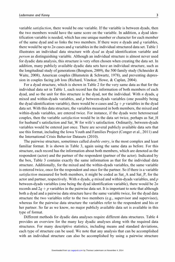
variable satisfaction, there would be one variable. If the variable is between dyads, then

the two members would have the same score on the variable. In addition, a dyad iden-

tification variable is needed, which has one unique number or character for each member

of the same dyad and so links the two members. If there were n dyads and q variables,

there would be up to 2n cases and q variables in the individual structured data set. Table 1

illustrates an individual data structure with dyad as dyad identification variable and

person as distinguishing variable. Although an individual structure is almost never used

for dyadic data analysis, this structure is very often chosen when creating the data set. In

addition, many publicly available dyadic data sets have an individual structure, such as

the longitudinal study of generations (Bengtson, 2009), the 500 family study (Schneider &

Waite, 2008), American couples (Blumstein & Schwartz, 1978), and preventing depres-

sion in couples facing job loss (Richard, Vinokur, Howe, & Caplan, 2004).

For a dyad structure, which is shown in Table 2 for the very same data as that for the

individual data set in Table 1, each record has the information of both members of each

dyad, and so the unit for this structure is the dyad, not the individual. With n dyads, q

mixed and within-dyads variables, and p between-dyads variables (one possibly being

the dyad identification variable), there would be n cases and 2qþ p variables in the dyad

data set. With this data structure, the variables measured in both members, the mixed and

within-dyads variables, are entered twice. For instance, if the dyads were heterosexual

couples, then the variable satisfaction would be in the data set twice, perhaps as Sat_H

for husband’s satisfaction and Sat_W for wife’s satisfaction. Ordinarily, between-dyads

variables would be entered just once. There are several publicly available data sets that

use this format, including the Iowa Youth and Families Project (Conger et al., 2011) and

the International Crisis Behavior Datasets (2010).

The pairwise structure, sometimes called double entry, is the most complex and least

familiar format. It is shown in Table 3, again using the same data as before. For this

structure, each record has the information about both members, which are denoted as the

respondent (actor) and the partner of the respondent (partner of the actor). Indicated by

the box, Table 3 contains exactly the same information as that for the individual data

structure. Additionally, for the mixed and the within-dyads variables, the same variable

is entered twice, once for the respondent and once for the partner. So if there is a variable

satisfaction measured for both members, it might be coded as Sat_A and Sat_P, for the

actor and partner, respectively. With n dyads, q mixed and within-dyads variables, and p

between-dyads variables (one being the dyad identification variable), there would be 2n

records and 2qþ p variables in the pairwise data set. It is important to note that although

both a dyad and a pairwise data structure have the same variable twice, for the dyad data

structure the two variables refer to the two members (e.g., supervisor and supervisee),

whereas for the pairwise data structure the variables refer to the respondent and his or

her partner. So far as we know, no major publicly available data set is available in this

type of format.

Different methods for dyadic data analyses require different data structures. Table 4

provides an overview for the many key dyadic analyses along with the required data

structures. For many descriptive statistics, including means and standard deviations,

each type of structure can be used. We note that any analysis that can be accomplished

with an individual structure can also be accomplished by using a pairwise structure

Ledermann and Kenny 3

by Thomas Ledermann on November 4, 2014spr.sagepub.comDownloaded from

because a pairwise data set includes an individual structure (see the box in Table 4). To

compare means and variances between distinguishable members, the use of the dyad

structure is most straightforward. To analyze correlations, the dyad structure is most

straightforward when dyad members are distinguishable, whereas in the indistinguish-

able case, the pairwise data structure is most straightforward, but the dyad structure can

be used with SEM and the impositions of equality constraints (Olsen & Kenny, 2006).

An often used measure for nonindependence is the intraclass correlation, which can be

most easily obtained using an individual or a pairwise data structure (see Alferes &

Kenny, 2009). For the analysis of associations between variables, two often-used meth-

ods of analysis are the APIM and the common fate model (CFM; Kenny & La Voie,

1985). The APIM can be analyzed by many statistical methods, including multiple

regression and SEM, which require a dyad data structure, or MLM, which uses a pairwise

Table 3. Example of a pairwise data structure (box indicates an individual data structure shown inTable 1).

Dyad Person Dur Com_A Sat_A Com_P Sat_P

1 1 3 5 9 2 81 2 3 2 8 5 92 1 7 6 3 4 62 2 7 4 6 6 33 1 5 3 6 9 73 2 5 9 7 3 6

Note. Com ¼ Commitment, Sat ¼ Satisfaction, Dur ¼ Relationship duration; A ¼ Actor, P ¼ Partner.

Table 1. Example of an individual data structure.

Dyad Person Com Sat Dur

1 1 5 9 31 2 2 8 32 1 6 3 72 2 4 6 73 1 3 6 53 2 9 7 5

Note. Com ¼ commitment; Sat ¼ satisfaction; Dur ¼ relationship duration.

Table 2. Example of a dyad data structure.

Dyad Dur Com_1 Sat_1 Com_2 Sat_2

1 3 5 9 2 82 7 6 3 4 63 5 3 6 9 7

Note. Com ¼ commitment; Sat ¼ satisfaction; Dur ¼ relationship duration; 1 ¼ Dyad Member 1; 2 ¼ DyadMember 2.

4 Journal of Social and Personal Relationships

by Thomas Ledermann on November 4, 2014spr.sagepub.comDownloaded from

data structure. The CFM can be analyzed using SEM or MSEM (Ledermann & Kenny,

2012). SEM requires a dyad data structure, whereas MSEM requires an individual or a

pairwise data structure. A third model is the mutual influence model (MIM; Kenny,

1996) that analyzes reciprocal effects between members. It requires the use of SEM and

a dyad data structure. Because the APIM estimated by MLM is currently used in most

analyses of associations between variables in dyadic research (Kenny & Kashy,

2014), researchers often face the task of creating a pairwise data set.

Typically, the format of the original data is of the either individual or dyad type.

However, most often we need to restructure the data to put it in the proper format before

we can analyze the data. Thus, data restructuring is a necessary but often a difficult task,

especially when a pairwise data set is required. Most computer packages do have options

to restructure data, but these methods are very often created for restructuring longitudinal

data. However, the restructuring of dyadic data are very different, and the restructuring

of an individual file into a pairwise file is very different from restructuring a dyad file

into a pairwise file. We also know that some users use ‘‘cut-and-paste’’ methods to

restructure dyadic data sets, which can easily lead to errors.2 Thus, having a toolbox with

programs that allows the user simply to go from one structure to another and distinguish

between-dyads variables from mixed and within-dyads variables would be very useful.

Additionally, none of the currently available methods provide any descriptive informa-

tion, which our programs do provide. For instance, knowing which variables are mixed,

between dyads, and within dyads can be very useful to a dyad researcher.

Programs to restructure dyadic data

There are three programs enabling the restructure of individual and dyad data sets and

that are part of the toolbox RDDD. Each program produces two files, one with the

restructured data set and the other with information about the variables in the data set.

Two of the programs also provide extensive descriptive statistics. These two programs

are ItoP, which changes an individual data set to a dyad data set, and ItoD, which changes

Table 4. Dyadic data analysis using different data structures.

Individual Dyad Pairwise

Descriptive statistics Yes Yes YesCorrelations No Yes YesICC Yes No YesAPIM using MLM No No YesAPIM using SEM No Yes NoAPIM using MR No Yes NoCFM using SEM No Yes NoCFM using MSEM Yes No YesMIM No Yes No

Note. APIM ¼ actor–partner interdependence model; CFM ¼ common fate model; ICC ¼ intraclass coefficient;MIM¼mutual influence model; MLM¼multilevel modeling; SEM¼ structural equation modeling; MR¼multipleregression analysis; MSEM ¼ multilevel SEM.

Ledermann and Kenny 5

by Thomas Ledermann on November 4, 2014spr.sagepub.comDownloaded from

an individual to a dyad data set. The third program is DtoP, which changes a dyad to a

pairwise or an individual data set.3 All the programs provide a graphical user interface

and can be downloaded from http://davidakenny.net/DyadR/RDDD.htm (to restructure

the data directly without using the graphical interfaces, R code is available at http://

thomasledermann.com/RDDD/). The programs offer several options to the users and are

relatively simple to use. Specifically, the programs identify variables that were measured

for both members and variables that were measured for only one member and variables

that are between-dyads variables. Currently, the programs can read a data set either in

‘‘sav’’ format (SPSS) or in ‘‘csv’’ format (comma separated text file). The restructured

data and the text file are saved to locations that are designated by the user. The restruc-

tured data is saved as a ‘‘csv’’ file and the text output as a ‘‘txt’’ file. Although the pro-

grams are written in R and so R has to be installed on the computer, no knowledge of R is

required for the user to run them but the installation of R and R packages. (Information

on how to install the programs and R can be found on the website using the links above.)

We now discuss each of the three programs, their data requirements, data input, and the

output. Although the three programs are stand-alone programs, they are integrated into

one single program called RDDD. Loading this program, users are first asked which of

the three programs should be run and then enter the information required for the selected

program.

ItoD

The program ItoD restructures an individual data set into a dyad data set and gives

descriptive statistics for individuals and descriptive and inferential statistics for dyads.

Data requirements. The input data set is an individual data set that needs to contain a dyad

identification variable and a distinguishing variable. If the name given for one of these

variables is not in the input data set, the program gives a message and stops. There can be

no more than two members per dyad, but some dyads may have the information from

only one member. If any group has more than two members, the program gives a

message and stops. All variables that are analyzed must be numeric variables; string

variables are allowed but are not analyzed.

Inputs. The program ItoD produces the input screen contained in Figure 1 that displays

the default values. The user tells the program the name and location of the data set as well

as the names of the dyad identification and distinguishing variables in that data set. In

addition, the user is asked for the suffixes that are to be added to the variables measured

in both members to denote member A and member B. For instance, ‘‘_H’’ and ‘‘_W’’

might be added at the end to each mixed or within-dyads variables if husbands and wives

were being studied. Alternatively, ‘‘.1’’ and ‘‘.2’’ could be used to distinguish the two

members. The user can also provide an optional list of variables that are used as labels

in the output text file. This list can include special characters and spaces, but the vari-

ables must be in the same order as the input data set. Additionally, the user designates

the location and name of both the dyad data set and the text file to be created.

6 Journal of Social and Personal Relationships

by Thomas Ledermann on November 4, 2014spr.sagepub.comDownloaded from

Output. The program creates two files. One is the restructured dyad data set which takes

each mixed and within-dyads variable and adds a suffix for each of the two dyad mem-

bers. Also included in the restructured data set are the between-dyads variables and the

dyad identification variable (always the first variable in the restructured data set).

The second output file is a text file that provides the following descriptive infor-

mation: the number of dyads and individuals of each type (both missing and list wise),

whether each variable in the data set is between, within, or mixed, and which variables

have no variance or fewer than five nonmissing cases. It also tells which variables might

be used as distinguishing variables. Then for each variable, it provides the mean, stan-

dard deviation, minimum and maximum values, and the intraclass correlation across

individuals. If there are missing data, it also gives the number of complete cases for that

variable.

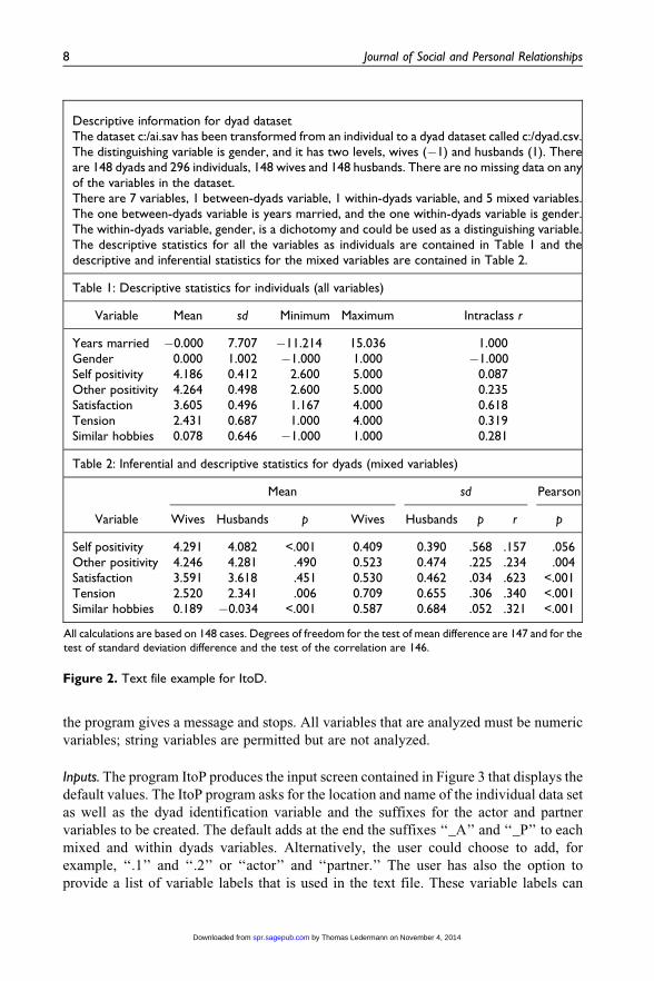
The program also produces both descriptive and inferential statistics for the dyad data

set. For each mixed variable, the mean and standard deviation for each of the two

members is provided and tests of the difference. Moreover, the Pearson correlation

between the two members is given and tested for statistical significance. We present an

example of the text file in Figure 2, which has one within-dyads variable (gender), one

between-dyads, and five mixed variables.

ItoP

The ItoP restructures an individual data set into a pairwise data set and provides

descriptive statistics of the variables in the data set.

Data requirements. As with the ItoD program, the input data set is an individual data set

that has a dyad identification variable. Again, if the name given for the dyad identifi-

cation variable is not in the input data set, the program gives a message and stops.

Moreover, there can be no more than two members per dyad, but some dyads may not

have information about the second member. If any group has more than two members,

Figure 1. Graphical user interface for the ItoD program.

Ledermann and Kenny 7

by Thomas Ledermann on November 4, 2014spr.sagepub.comDownloaded from

the program gives a message and stops. All variables that are analyzed must be numeric

variables; string variables are permitted but are not analyzed.

Inputs. The program ItoP produces the input screen contained in Figure 3 that displays the

default values. The ItoP program asks for the location and name of the individual data set

as well as the dyad identification variable and the suffixes for the actor and partner

variables to be created. The default adds at the end the suffixes ‘‘_A’’ and ‘‘_P’’ to each

mixed and within dyads variables. Alternatively, the user could choose to add, for

example, ‘‘.1’’ and ‘‘.2’’ or ‘‘actor’’ and ‘‘partner.’’ The user has also the option to

provide a list of variable labels that is used in the text file. These variable labels can

Descriptive information for dyad datasetThe dataset c:/ai.sav has been transformed from an individual to a dyad dataset called c:/dyad.csv.The distinguishing variable is gender, and it has two levels, wives (�1) and husbands (1). Thereare 148 dyads and 296 individuals, 148 wives and 148 husbands. There are no missing data on anyof the variables in the dataset.There are 7 variables, 1 between-dyads variable, 1 within-dyads variable, and 5 mixed variables.The one between-dyads variable is years married, and the one within-dyads variable is gender.The within-dyads variable, gender, is a dichotomy and could be used as a distinguishing variable.The descriptive statistics for all the variables as individuals are contained in Table 1 and thedescriptive and inferential statistics for the mixed variables are contained in Table 2.

Table 1: Descriptive statistics for individuals (all variables)

Variable Mean sd Minimum Maximum Intraclass r

Years married �0.000 7.707 �11.214 15.036 1.000Gender 0.000 1.002 �1.000 1.000 �1.000Self positivity 4.186 0.412 2.600 5.000 0.087Other positivity 4.264 0.498 2.600 5.000 0.235Satisfaction 3.605 0.496 1.167 4.000 0.618Tension 2.431 0.687 1.000 4.000 0.319Similar hobbies 0.078 0.646 �1.000 1.000 0.281

Table 2: Inferential and descriptive statistics for dyads (mixed variables)

Mean sd Pearson

Variable Wives Husbands p Wives Husbands p r p

Self positivity 4.291 4.082 <.001 0.409 0.390 .568 .157 .056Other positivity 4.246 4.281 .490 0.523 0.474 .225 .234 .004Satisfaction 3.591 3.618 .451 0.530 0.462 .034 .623 <.001Tension 2.520 2.341 .006 0.709 0.655 .306 .340 <.001Similar hobbies 0.189 �0.034 <.001 0.587 0.684 .052 .321 <.001

All calculations are based on 148 cases. Degrees of freedom for the test of mean difference are 147 and for thetest of standard deviation difference and the test of the correlation are 146.

Figure 2. Text file example for ItoD.

8 Journal of Social and Personal Relationships

by Thomas Ledermann on November 4, 2014spr.sagepub.comDownloaded from

include special characters and spaces, but the variables must be in the same order as the

input data set.

Output. The program creates two files. One is the restructured data set. That file takes

each mixed and within-dyads variable and gives the actor and partner values for each

person. Also included in the restructured data set are the between-dyads variables and

the dyad identification variable (always the first variable in the new data set). Addition-

ally, the program creates a within-dyads variable called partnum, which arbitrarily

assigns a ‘‘1’’ to the first member of the dyad and a ‘‘2’’ to the second. For dyads in which

there is information for only one member, a second record is created for the missing

member. These new members have the dyad identification variable and values are

imputed for any between- and within-dyads variable if the score on that variable is not

missing for the other member. Missing scores for a mixed variable are not imputed. The

program adds a new between-dyads variable called Solo, which denotes those cases for

which only one of the two members is measured. The imputation of within- and between-

dyads variables is also done for cases in which both members of the dyad are measured,

and there is a within- or between-dyads variable for only one of the two members.

The program also creates a text file that provides the following descriptive infor-

mation: the number of dyads and individuals and whether each variable in the data set is

between, within, or mixed. It also informs what variables, if any, might be used as

distinguishing variables. Then for each variable it gives the mean, standard deviation,

minimum and maximum values, and the intraclass correlation. If there are missing data,

it also gives the number of complete cases for that variable. The text file also notes what

variables have no variance and have fewer than five cases.

DtoP

The program DtoP restructures a dyad data set into either a pairwise data set or an

individual data set.

Figure 3. Graphical user interface for the ItoP program.

Ledermann and Kenny 9

by Thomas Ledermann on November 4, 2014spr.sagepub.comDownloaded from

Data requirements. The input data set is a dyad data set. In this data set, there is infor-

mation in the variable name for each mixed variable about the member to which the

variable refers. That information about the member can either be at the end or the

beginning of the stem of the variable name. Consistent with the requirements of most

statistical programs, the first character of the variable name must be a letter, numbers or

symbols are not permitted. In addition, the program can handle separators, such as points

or slashes, between the stem of the variable name and the information of the dyad

member. For instance, the program can handle the following examples of pairs of

variable names: <X_female and X_male>, <sat.W and sat.H>, <wDepr and hDepr>, and

<mom_x and dad_x>. It is permissible, that for some variables, only one of the two

members has a value, for example, there might be a mom_pregnant variable but no

dad_pregnant variable. If the stem of a mixed variable is the same as the variable name

for a between-dyads variable (e.g., X_male and X) the program gives a message and

stops.

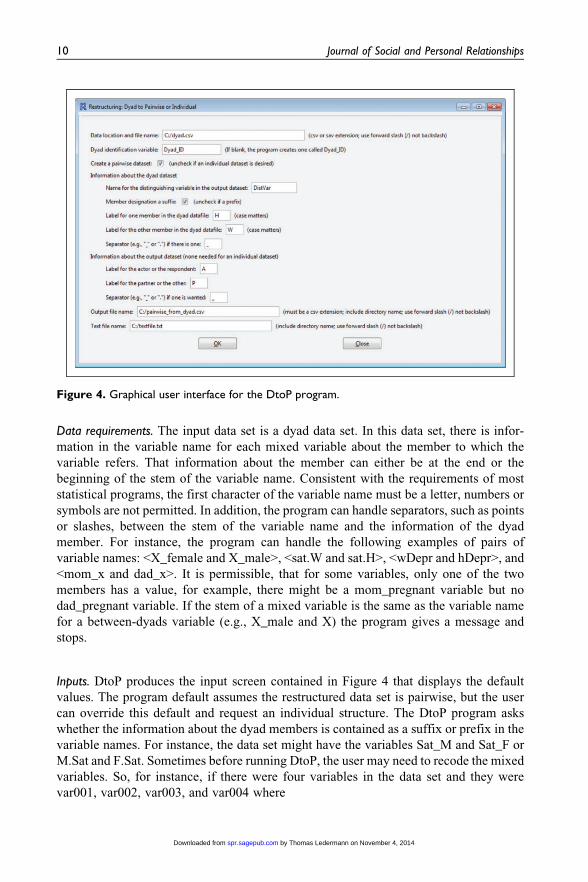
Inputs. DtoP produces the input screen contained in Figure 4 that displays the default

values. The program default assumes the restructured data set is pairwise, but the user

can override this default and request an individual structure. The DtoP program asks

whether the information about the dyad members is contained as a suffix or prefix in the

variable names. For instance, the data set might have the variables Sat_M and Sat_F or

M.Sat and F.Sat. Sometimes before running DtoP, the user may need to recode the mixed

variables. So, for instance, if there were four variables in the data set and they were

var001, var002, var003, and var004 where

Figure 4. Graphical user interface for the DtoP program.

10 Journal of Social and Personal Relationships

by Thomas Ledermann on November 4, 2014spr.sagepub.comDownloaded from

var001: husband satisfaction,

var002: wife satisfaction,

var003: husband commitment, and

var004: wife commitment,

these variables would have to be recoded, perhaps as sat_H, sat_W, com_H, and

com_W or alternatively as h.sat, w.sat, h.com, and w.com before running DtoP. For this

example, gender would be the implicit distinguishing variable and users would provide

this name on the graphical interface. As with ItoP, the program adds suffixes for the actor

and partner variables. The default are ‘‘_A’’ and ‘‘_P,’’ which are added to the stem of

each mixed or within-dyads variable. However, the user can override these defaults and

use something else, for example, ‘‘.1’’ and ‘‘.2.’’ The program also asks the name of the

implicit distinguishing variable (e.g., gender), and the user also has the option to

restructure the dyad data set into an individual data set instead of a pairwise data set.

Output. DtoP creates the pairwise or individual data set and the text file. The pairwise

data set has for each paired variable an actor and a partner variable. Additionally, the

distinguishing variable is added using for the prefix or suffix the values from the dyad

data set (e.g., H and W). If the distinguishing information is a string variable, an addi-

tional numeric distinguishing variable is added that has 1 for the first level and 2 for the

second and the same name as the original variable plus ‘‘_numeric’’ as a suffix. Also a

short text file is produced that describes the dyad data set and the new data set. However,

unlike the other programs, it does not provide any descriptive or inferential statistics.

Note though that if an individual data set were to be created, then the descriptive sta-

tistics could be obtained by restructuring it using ItoD or ItoP.

Restructuring longitudinal dyadic data

We now turn to the restructuring of multiwave dyadic data and the use of MLM, SEM,

and MSEM, which all require a different data structure.

MLM analysis

MLM typically requires the data to be organized in what is called a person-period data

structure (Singer & Willett, 2003) where each record has the information of one member

at one time point. With n dyads and q mixed variables each measured in both members at

t occasions, there would be 2nt cases and q mixed variables plus a dyad identification

variable, a distinguishing variable, and a time variable in the data set. This structure

permits the analysis of growth processes in dyads (Raudenbush, Brennan, & Barnett,

1995). The analysis of actor and partner effects in longitudinal data requires a pairwise

person-period data set with 2nt cases and 2q mixed variables (see Kashy & Donnellan,

2012). Such a data set can be created using ItoP when the original data set is already of

the type person-period. To do so, the dyad identification variable would be the unique

time point, not dyad. So if there are 10 dyads and 3 time points, we might multiply the

Ledermann and Kenny 11

by Thomas Ledermann on November 4, 2014spr.sagepub.comDownloaded from

dyad identification variable by 10 and then add the time point (1–3) to create a new

‘‘dyad’’ identification variable.

However, when the original data set has a dyad structure where each record has the

information of both members and all measurement points (i.e., a data set with n cases

and 2qt variables), the data can be restructured using DtoP and built-in procedures of

standard statistical software programs for restructuring longitudinal data (e.g., the

restructure data wizard in SPSS enables either the restructuring of selected variables

into cases or the restructuring of selected cases into variables). In a dyad data set, each

mixed variable name has the information of the member and the time point. The infor-

mation of the member can be before or after the information of the measurement occa-

sion. If this information is either a suffix or prefix, there are four possible

combinations. For a variable satisfaction measured at three occasions in both members,

the four possibilities are:

Sat_1M, Sat_2M, Sat_3M, Sat_1F, Sat_2F, Sat_3F;

Sat_M1, Sat_M2, Sat_M3, Sat_F1, Sat_F2, Sat_F3;

M1_Sat, M2_Sat, M3_Sat, F1_Sat, F2_Sat, F3_Sat; and

aM_Sat, bM_Sat, cM_Sat, aF_Sat, bF_Sat, cF_Sat.

It is important to note that most statistical software programs require that the first

character to be a ‘‘string.’’ Thus, a, b, and c (and not 1, 2, and 3) were used for the

three time points in the last example. The restructuring can be done in two steps

using our program and standard procedures. The order of the information determines

whether one should use first DtoP or standard procedures for restructuring long-

itudinal data. DtoP would be used if the member information is the final suffix or

the first prefix (first and third example, i.e., Sat_1M or M1_Sat) in order to create an

individual data set with 2n cases and qt variables. This data set can then be turned

into a person-period data set using standard procedures for restructuring longitudinal

data. If the time information is the final suffix or the first prefix (second and fourth

example, i.e., Sat_M1 or aM_Sat) the built-in procedure for restructuring longitudi-

nal data would be used first and then DtoP to restructure the data into a person-

period pairwise data set for MLM analysis.

SEM analysis

The use of SEM for longitudinal dyadic analysis requires a data set to be organized what

can be called a dyad person-level data set, in which there would be n cases and 2qt mixed

variables. If the original data format is of the form person-period a dyad person-level

data set can be created using ItoD and built-in procedures for restructuring longitudinal

data. The order in which the procedures are used determines whether the suffix in the

dyad person-level data set begins with the information of the member or with the infor-

mation of the time point. For example, using first ItoD and then the procedures for long-

itudinal data, the suffix in the final data set begins with the information of the member

followed by the information of the time point.

12 Journal of Social and Personal Relationships

by Thomas Ledermann on November 4, 2014spr.sagepub.comDownloaded from

MSEM analysis

MSEM can be used to analyze growth at the dyadic (group) level (Ledermann & Macho,

2014). The data structure is such that the information of each member is contained in a

single record. With n dyads and q mixed variables measured t times, there would be 2n

records and qt mixed variables (see Ledermann & Macho, 2014, for an example data set).

If the original data structure is of the form dyad, DtoP can be used choosing the option to

create an individual data set.

Limitations, extensions, and further directions

We have described a toolbox with programs for restructuring dyadic data and for cal-

culating descriptive and inferential statistics. The graphical user interface and the

minimum of input information required make the programs user friendly. We have also

provided guidance to restructure longitudinal dyadic designs for the use of MLM, SEM,

or MSEM. For data sets with many variables, the output with the descriptive statistics

can become very large, and so it might be advisable to select a subset of variables before

restructuring the data.

The programs are not without limitations. One limitation is that in some situations the

restructuring of overtime dyadic data requires a sequential use of the programs described in

this article and built-in procedures in standard software programs for restructuring longi-

tudinal data. The use of both the programs for dyadic data and the procedures for longitu-

dinal data enables the restructuring of almost any hierarchical organized data. Moreover,

our own experience is that the built-in procedures in standard software statistic programs

are handy for restructuring overtime data, and most researchers have almost no problems

with the use of them. Another limitation is that the programs were also designed for the

standard design: each person is paired with one partner. For both social relations and

one-with-many designs (Kenny et al., 2006), we can use ItoP to create pairwise data sets,

as long as the dyad identification variable refers to one pair of persons. A final limitation is

that in the dyad data file the information about the members (e.g., M or F) needs to already

be at the beginning or at the end of the names of the variables measured in both members.

If not, the mixed variables need to renamed before running the program.

We envision that other toolboxes will be created. We would expect that very soon

there would be one with programs to estimate the APIM, CFM, and MIM. A prototype is

currently available at http://davidkenny.net/DyadR/DyadR.htm. Each of these programs

would produce not only standard computer output but also text output describing the

results. Because R is open source, we encourage other researchers to join us in building

this toolbox for relationship researchers.

Acknowledgment

We thank William Cook for helpful comments on an earlier version of this article.

Funding

This research received no specific grant from any funding agency in the public, commercial, or

not-for-profit sectors.

Ledermann and Kenny 13

by Thomas Ledermann on November 4, 2014spr.sagepub.comDownloaded from

Notes

1. In the longitudinal analysis literature, the individual structure is sometimes referred to as a long

format and the dyad structure is referred to as a wide format.

2. There are two SPSS macros that restructure individual to either pairwise or dyadic structures

(http://davidakenny.net/kkc/c1/restructure.htm).

3. Restructuring from pairwise to individual and from pairwise to dyad is relatively trivial in that

cases or variables just need to be deleted and variables need to be renamed.

References

Alferes, V. R., & Kenny, D. A. (2009). SPSS programs for the measurement of nonindependence

in standard dyadic designs. Behavior Research Methods, 41, 47–54. doi:10.3758/BRM.41.1.47

Bengtson, V. L. (2009). Longitudinal study of generations, 1971, 1985, 1988, 1991, 1994, 1997,

2000. ICPSR22100-v2. Ann Arbor, MI: Inter-University Consortium for Political and Social

Research [distributor]. doi:10.3886/ICPSR04076.v1

Blumstein, P., & Schwartz, P. (1978). American couples (dataset form). Radcliffe College, Cam-

bridge, MA.

Conger, R. D., Lasley, P., Lorenz, F. O., Simons, R., Whitbeck, L. B., Elder, G. H. Jr., & Norem, R.

(2011). Iowa youth and bibliographic citation: Families project, 1989-1992. ICPSR26721-v2.

Ann Arbor, MI: Inter-university Consortium for Political and Social Research [distributor],

2011-11-03. doi:10.3886/ICPSR26721.v2

International Crisis Behavior Datasets: Version 10 (1918-2007). (2010). Center for International

Development and Conflict Management, University of Maryland. Retrieved from http://www.

cidcm.umd.edu/icb/data/icb%20version%2010%20release%20memo.pdf

Kashy, D. A., & Donnellan, M. B. (2012). Conceptual and methodological issues in the anal-

ysis of data from dyads and groups. In K. Deaux & M. Snyder (Eds.), The Oxford hand-

book of personality and social psychology (pp. 209–238). New York, NY: Oxford

University Press.

Kenny, D. A. (1996). Models of non-independence in dyadic research. Journal of Social and Per-

sonal Relationships, 13, 279–294. doi:10.1177/0265407596132007

Kenny, D. A., & Kashy, D. A. (2014). The design and analysis of data from dyads and groups. In

H. T. Reis & C. M. Judd (Eds.), Handbook of research methods in social and personality psy-

chology (2nd ed., pp. 589–607). New York, NY: Cambridge University Press.

Kenny, D. A., Kashy, D. A., & Cook, W. L. (2006). Dyadic data analysis. New York, NY: Guil-

ford Press.

Kenny, D. A., & La Voie, L. (1985). Separating individual and group effects. Journal of Person-

ality and Social Psychology, 48, 339–348. doi:10.1037/0022-3514.48.2.339

Ledermann, T., & Kenny, D. A. (2012). The common fate model for dyadic data: Variations of a

theoretically important but underutilized model. Journal of Family Psychology, 26, 140–148.

doi:10.1037/a0026624

Ledermann, T., & Macho, S. (2014). Analyzing change at the dyadic level: The common fate

growth model. Journal of Family Psychology, 28, 204–213. doi:10.1037/a0036051

Olsen, J. A., & Kenny, D. A. (2006). Structural equation modeling with interchangeable dyads.

Psychological Methods, 11, 127–141. doi:10.1037/1082-989x.11.2.127

14 Journal of Social and Personal Relationships

by Thomas Ledermann on November 4, 2014spr.sagepub.comDownloaded from

Raudenbush, S. W., Brennan, R. T., & Barnett, R. C. (1995). A multivariate hierarchical model for

studying psychological change within married couples. Journal of Family Psychology, 9,

161–174. doi:10.1037/0893-3200.9.2.161

Richard, P. H., Vinokur, A. D., Howe, G. W., & Caplan, R. D. (2004). Prevention depression in

couples facing job loss, 1996-1998: [Baltimore, Maryland, and Detroit, Michigan] [Computer

file]. ICPSR version. Ann Arbor, MI: Institute for Social Research, Survey Research Center,

and Michigan Prevention Research Center/Washington, DC: George Washington University,

Center for Family Research [producers], 1998. Ann Arbor, MI: Inter-University Consortium

for Political and Social Research [distributor].

R Core Team. (2014). R: A language and environment for statistical computing. Vienna, Austria:

R Foundation for Statistical Computing. Retrieved from http://www.R-project.org/

Schneider, B., & Waite, L. J. (2008). The 500 family study [1998-2000: United States]. Ann Arbor,

MI: Inter-university Consortium for Political and Social Research [distributor].

Singer, J. D., & Willett, J. B. (2003). Applied longitudinal data analysis: Modeling change and

event occurrence. New York, NY: Oxford University Press.

Ledermann and Kenny 15

by Thomas Ledermann on November 4, 2014spr.sagepub.comDownloaded from