lable at ScienceDirect

Journal of Rock Mechanics and Geotechnical Engineering 9 (2017) 135e149

Contents lists avai

Journal of Rock Mechanics andGeotechnical Engineering

journal homepage: www.rockgeotech.org

Full Length Article

Generalized stress field in granular soils heap with RayleigheRitzmethod

Gang Bi a,b

aCH2M, Inc., Englewood, USAbChongqing Titan Architects-Multi-Disciplinary Practice Co., Chongqing, China

a r t i c l e i n f o

Article history:Received 3 March 2016Received in revised form28 April 2016Accepted 16 July 2016Available online 8 December 2016

Keywords:Generalized stress fieldRayleigheRitz methodStress depressionVariation of the functionPrinciple of minimum potential energy

E-mail address: gblvzl@gmail.com.Peer review under responsibility of Institute o

Chinese Academy of Sciences.

http://dx.doi.org/10.1016/j.jrmge.2016.07.0071674-7755 � 2017 Institute of Rock and Soil MechanicNC-ND license (http://creativecommons.org/licenses/b

a b s t r a c t

The stress field in granular soils heap (including piled coal) will have a non-negligible impact on thesettlement of the underlying soils. It is usually obtained by measurements and numerical simulations.Because the former method is not reliable as pressure cells instrumented on the interface between piledcoal and the underlying soft soil do not work well, results from numerical methods alone are necessaryto be doubly checked with one more method before they are extended to more complex cases. Thegeneralized stress field in granular soils heap is analyzed with RayleigheRitz method. The problem isdivided into two cases: case A without horizontal constraint on the base and case B with horizontalconstraint on the base. In both cases, the displacement functions u(x, y) and v(x, y) are assumed to becubic polynomials with 12 undetermined parameters, which will satisfy the Cauchy’s partial differentialequations, generalized Hooke’s law and boundary equations. A function is built with the RayleigheRitzmethod according to the principle of minimum potential energy, and the problem is converted intosolving two undetermined parameters through the variation of the function, while the other parametersare expressed in terms of these two parameters. By comparison of results from the RayleigheRitzmethod and numerical simulations, it is demonstrated that the RayleigheRitz method is feasible to studythe generalized stress field in granular soils heap. Solutions from numerical methods are verified beforebeing extended to more complicated cases.� 2017 Institute of Rock and Soil Mechanics, Chinese Academy of Sciences. Production and hosting byElsevier B.V. This is an open access article under the CC BY-NC-ND license (http://creativecommons.org/

licenses/by-nc-nd/4.0/).

1. Introduction

In recent years, as the economy of China continues to grow, aplenty of power plants are constructed where soft clay is verycommon. One aspect of the concerns is the settlement of soft clayassociated with the above piled coal, which is used in fuel powerplants. It may be assumed that the normal stress distribution at theinterface between piled coal and underlying soft clay is linear,however, it is not always true. It was first observed by physiciansthrough experiments (Herrmann et al., 2013; Pipatpongsa et al.,2014) in the desert that the peak vertical force at the base doesnot occur directly beneath the vertex of the piled sand, but at someintermediate points, which may also be called the arching phe-nomenon (or stress depression, stress dip). Many physicians havetried to explain the behavior of piled sand. Ai et al. (2013) believed

f Rock and Soil Mechanics,

s, Chinese Academy of Sciences. Pry-nc-nd/4.0/).

that the deposition process is directly related to this behavior.Bouchaud et al. (1995) and Savage (1997) proposed a nonlinearwave equation to describe how forces propagate within a granularmedium. Cates et al. (1998) and Vanel et al. (1999, 2000) attemptedto explain this phenomenon by invoking local rules for stresspropagation that depend on the construction history of the sand-pile. Edwards and Grinev (1999) put forward a statisticaleme-chanical theory of stress transmission in disordered arrays of rigidgrains with perfect friction.

The piled coal is quite similar to the piled sand, while onedimension is much larger than the other two dimensions in bothcases. The cross-section of piled sand is usually triangular, and thatof piled coal is normally trapezoidal. Nevertheless, the trapezoidcould be divided into a triangle and a rectangle, or taken as a tri-angle if the height of the trapezoid is greater than the topline. Ineither case, it is necessary to focus the stress field in the piled coalwith the triangular cross-section.

Measurements in project sites and numerical simulations arethe two main methods. However, instrumentations (like pressure

oduction and hosting by Elsevier B.V. This is an open access article under the CC BY-

Fig. 1. Granular soils heap.

Fig. 2. Case A without horizontal constraint on the base.

Fig. 3. Case B with horizontal constraint on the base.

G. Bi / Journal of Rock Mechanics and Geotechnical Engineering 9 (2017) 135e149136

cells) on soft clay do not work well. Results from numericalmethods alone are needed to be doubly checked with those fromthe third way. Many researchers have tried to acquire the theo-retical solution of stress field in the piled sand, and it is notpossible without making an additional postulate. Angelillo et al.(2016) presumed granular material behaving like the continuumbut governed by MohreCoulomb yield condition. Bi et al. (2014,2016) assumed that the principal stress axes have a fixed angleof inclination with the vertical direction. Matuttis and Schinner(1999) and Matuttis et al. (2000) computed the pressure distri-bution under wedges using linear superposition for given pressuredistributions. Watson (1996) proposed that the main compressivestresses lie along fixed parallel lines, which steer the pile’s weightaway from the center, giving a central pressure dip. Zhu et al.(2013) concerned the impact of the particle aspect ratio onstress dip.

It is a long debate whether elasticity theory and continuumtheory could be able to explain the stress field in the piled sand (orcoal). Cox (2001), Hill and Cox (2000, 2002) and Liffman et al.(1999) tried to estimate the horizontal and vertical force distribu-tions using the proper continuum mechanical theory of granularmaterials. Da Silva and Rajchenbach (2000) stated that collectionsof elastic grains subjected to a compressive load will behave elas-tically. And the presented results were based on a two-dimensionalmodel system, made of discrete square cells submitted to a pointload, in which the region where the stress is confined is photo-elastically visualized as a parabola. Krimer et al. (2006) andSokolovskii (2013) argued that granular materials are predomi-nantly plastic, incrementally nonlinear, preparation-dependent,and anisotropic under shearing. Nevertheless, their static stressdistribution is well accounted for, in the whole range up to thepoint of failure, by a judiciously tailored isotropic nonanalyticelasticity theory termed granular elasticity. Zheng and Yu (2014)claimed that they have found why previous researches based oncontinuum theory failed on stress depression.

However, understanding the mechanical properties of granularmaterials is important not only for physical sciences, but also forapplications in geotechnical engineering. Though the stress distri-bution on the base to calculate settlement follows the linearassumption made by Osterberg (1957), geotechnical researchershave involved this nonlinear distribution long time ago. The way toderive the coefficient of earth pressure at rest by Jaky (1944) hasimplicitly assumed that the normal stress on the base is nonlinearwith height. Bishop (1967) stated that this nonlinear stress distri-bution caused the progressive failure of slopes and landslides.Michalowski and Park (2004, 2005) studied the phenomenonobserved from the approach of limit analysis.

The author believes that the solutions based on elasticity theorywill at least be feasible to provide the guide for the research on thestress field in piled coal. And the approximate solution with Ray-leigheRitz method in this article aims to doubly check the resultsfrom numerical methods. Then numerical solutions could be trus-ted to be extended tomore complex cases where the classicmethodis unable to be relied on.

2. Theoretical solutions of two cases

Considering the infinite granular soils heap as shown in Fig. 1,the stress state of any points inside and/or at the boundary of theheap can be obtained by simplifying the problem into two cases:case A without horizontal constraint at the base (Fig. 2) and case Bwith horizontal constrain at the base (Fig. 3).

According to the elasticity theory, the Cauchy’s partial differ-ential equations can be written as

E2ð1þ mÞ

"1

1� 2m

v2u

vx2þ v2v

vxvy

!þ v2u

vx2þ v2u

vy2

#¼ 0

E2ð1þ mÞ

"1

1� 2m

v2v

vy2þ v2uvxvy

!þ v2v

vx2þ v2v

vy2

#þ g ¼ 0

9>>>>>=>>>>>;

(1)

where u ¼ u(x, y) is the horizontal displacement (also x-displace-ment) of any points; v ¼ v(x, y) is the vertical displacement (also y-displacement) of any points; E is the Young’s modulus; m is thePoisson’s ratio; and g is the unit weight.

For the case A (Fig. 2) and case B (Fig. 3), according to thegeneralized Hooke’s law, the following equation can be obtained:

G. Bi / Journal of Rock Mechanics and Geotechnical Engineering 9 (2017) 135e149 137

sx ¼ E

1� m2�εx þ mεy

�

sy ¼ E

1� m2�mεx þ εy

�

sxy ¼ E2ð1þ mÞ

�vuvy

þ vv

vx

�

9>>>>>>>>=>>>>>>>>;

(2)

where sx ¼ sx(x, y) is the horizontal normal stress of any surfaces;sy ¼ sy(x, y) is the vertical normal stress of any surfaces; sxy ¼ sxy(x,y) is the shear stress of any surfaces; εx ¼ εxðx; yÞ ¼ vuðx; yÞ=vx isthe horizontal strain of any points; and εy ¼ εyðx; yÞ ¼ vvðx; yÞ=vxis the vertical strain of any points.

Whist the boundary equations of case A are

ðuÞx¼0 ¼ 0; ðvÞy¼0 ¼ 0�sxy�x¼0 ¼ 0;

�sxy�y¼0 ¼ 0

sin aðsxÞy¼�x tan aþh þ cos a�sxy�y¼�x tan aþh ¼ 0

cos a�sy�y¼�x tan aþh þ sin a

�sxy�y¼�x tan aþh ¼ 0

9>>>=>>>;

(3)

where a is the angle of the slope (see Figs. 2 and 3).The boundary equations of case B are

ðuÞx¼0 ¼ 0; ðvÞy¼0 ¼ 0�sxy�x¼0 ¼ 0; ðuÞy¼0 ¼ 0

sin aðsxÞy¼�x tan aþh þ cos a�sxy�y¼�x tan aþh ¼ 0

cos a�sy�y¼�x tan aþh þ sin a

�sxy�y¼�x tan aþh ¼ 0

9>>>=>>>;

(4)

However, it is almost impossible to acquire the analyticalexpression of stress field of the heap by combining Eqs. (1)e(4). Theapproximate solution of the analytical expression is obtained withthe RayleigheRitz method in the subsequent section.

3. Approximate solutions with RayleigheRitz method

The procedure to obtain the analytical solution of stress field ofthe heap with the RayleigheRitz method is as follows:

(1) Assume the expressions of u(x, y) and v(x, y);(2) Combine the expressions with the boundary equations (Eqs.

(3) and (4)) to reduce the undetermined parameters in theexpressions;

(3) Build the function P ¼ RRU½sijεij=2� rvðx; yÞ�dxdy;

(4) According to the principle of minimum potentialenergy, solve the built function to acquire undeterminedparameters.

3.1. Analytical solution with RayleigheRitz method, case A

Here u(x, y) and v(x, y) are assumed to be cubic polynomials:

u ¼ x�a1 þ a2xþ a3yþ a4x

2 þ a5xyþ a6y2�

(5)

v ¼ y�b1 þ b2xþ b3yþ b4x

2 þ b5xyþ b6y2�

(6)

The displacement boundary in Eq. (3) has already been satisfiedin the assumed polynomials.

Combining with Eq. (2), the shear stress will be

sxy ¼ E2ð1þ mÞ

�vuvy

þ vv

vx

�

¼ E2ð1þ mÞ

�a3xþ a5x

2 þ 2a6xyþ b2yþ 2b4xyþ b5y2�

(7)

Then, combining the stress boundary in Eq. (3) can obtain:

�sxy�x¼0 ¼ 0 0b2 ¼ 0; b5 ¼ 0�

sxy�y¼0 ¼ 0 0a3 ¼ 0; a5 ¼ 0

)(8)

The assumed polynomials are simplified as

u ¼ x�a1 þ a2xþ a4x

2 þ a6y2�

(9)

v ¼ y�b1 þ b3yþ b4x

2 þ b6y2�

(10)

Combining Eq. (1), the strain will be

εx ¼ vuvx

¼ a1 þ 2a2xþ 3a4x2 þ a6y

2 (11)

εy ¼ vv

vy¼ b1 þ 2b3yþ b4x

2 þ 3b6y2 (12)

gxy ¼ vuvy

þ vv

vx¼ 2a6xyþ 2b4xy (13)

where g ¼ g(x, y) is the shear strain of any points.Substituting Eqs. (11)e(13) into Eq. (2), the stresses can be

obtained:

1�m2

Esx ¼ a1þ2a2xþ3a4x

2þa6y2þm

�b1þ2b3yþb4x

2

þ3b6y2�

(14)

1�m2

Esy ¼ b1þ2b3yþb4x

2þ3b6y2þm

�a1þ2a2xþ3a4x

2

þa6y2�

(15)

1� m2

Esxy ¼ ð1� mÞða6 þ b4Þxy (16)

Combining Eqs. (14)e(16) with the stress boundary conditionsin Eq. (3), and reorganizing the equations following the descendingpower of x, six equations in total can be acquired with two unde-termined parameters. Then, these two parameters will be deter-mined through the variation of the function as follows:

a6 :¼ðC26C27 þ C22C27 þ C18C27 � C28C16 � C28C20 � C28C24Þ=ð � C15C18 � C15C22 � C15C26 � C19C18 � C19C22 � C19C26� C23C18 � C23C22 � C23C26 þ C16C17 þ C16C21 þ C16C25þ C20C17 þ C20C21 þ C20C25 þ C24C17 þ C24C21 þ C24C25Þ

(17)

G. Bi / Journal of Rock Mechanics and Geotechnical Engineering 9 (2017) 135e149138

b6 : ¼ ðC15C28 þ C19C28 þ C23C28 � C27C17 � C27C21 � C27C25Þ=ð � C15C18 � C15C22 � C15C26 � C19C18 � C19C22 � C19C26� C23C18 � C23C22 � C23C26 þ C16C17 þ C16C21 þ C16C25þ C20C17 þ C20C21 þ C20C25 þ C24C17 þ C24C21 þ C24C25Þ

(18)

Other parameters are expressed in terms of a6 and b6:

a1 :¼ C1a6; b1 :¼ C7a6 þ C8b6a2 :¼ C3a6 þ C4b6;b3 :¼ C9a6 þ C10b6a4 :¼ C5a6 þ C6b6;b4 :¼ C11a6 þ C12b6

9=; (19)

So, the expressions of u(x, y) and v(x, y) are

u :¼ xhC1a6 þ ðC3a6 þ C4b6Þxþ ðC5a6 þ C6b6Þx2 þ a6y

2i

(20)

v :¼ yhC7a6þC8b6þðC9a6þC10b6ÞyþðC11a6þC12b6Þx2þb6y

2i

(21)

The whole process of variation of the function for case A ispresented in Appendix, which includes the expression of C1eC28.

Now, substituting Eqs. (20) and (21) into the functionP ¼ RR

U½sijεij=2� rvðx; yÞ�dxdy built with the RayleigheRitzmethod (Step 3 mentioned above), a6 and b6 can be known bydifferentiation of the function with respect to a6 and b6.

3.2. Analytical solution with RayleigheRitz method, case B

In this case, u(x, y) and v(x, y) are also assumed to be cubicpolynomials:

u ¼ xyða1 þ a2xþ a3yÞ (22)

v ¼ y�b1 þ b2xþ b3yþ b4x

2 þ b5xyþ b6y2�

(23)

The displacement boundary in Eq. (4) has already been satisfiedin the assumed polynomials.

Combining with Eq. (2), the shear stress will be

sxy ¼ E2ð1þ mÞ

�vuvy

þ vv

vx

�

¼ E2ð1þ mÞ

�a1xþ a2x

2 þ 2a3xyþ b2yþ 2b4xyþ b5y2�(24)

Then, combining the stress boundary conditions in Eq. (4) yields�sxy�x¼0 ¼ 0 0b2 ¼ 0; b5 ¼ 0 (25)

The assumed polynomials are simplified as

u ¼ xyða1 þ a2xþ a3yÞ (26)

v ¼ y�b1 þ b3yþ b4x

2 þ b6y2�

(27)

Combining Eq. (1), the strains will be

εx ¼ vuvx

¼ a1yþ 2a2xyþ a3y2 (28)

εy ¼ vv

vy¼ b1 þ 2b3yþ b4x

2 þ 3b6y2 (29)

gxy ¼ vuvy

þ vv

vx¼ a1xþ a2x

2 þ 2a3xyþ 2b4xy (30)

Again, substituting Eqs. (28)e(30) into Eq. (2), the stresses canbe obtained as follows:

1� m2

Esx ¼ a1yþ 2a2xyþ a3y

2 þ m�b1 þ 2b3yþ b4x

2 þ 3b6y2�

(31)

1� m2

Esy ¼ b1 þ 2b3yþ b4x

2 þ 3b6y2 þ m

�a1yþ 2a2xyþ a3y

2�

(32)

1� m2

Esxy ¼ 1� m

2

�a1xþ a2x

2 þ 2a3xyþ 2b4xy�

(33)

Combining Eqs. (31)e(33) with the stress boundary conditionsin Eq. (4), and reorganizing equations following the descendingpower of x, six equations in total will be acquired with two unde-termined parameters. Then, these two parameters can be deter-mined through the variation of the function as follows:

a3 : ¼ ðC26C27 þ C22C27 þ C18C27 � C28C16 � C28C24 � C28C20Þ=ð � C15C18 � C15C22 � C15C26 � C19C18 � C19C22 � C19C26� C23C18 � C23C22 � C23C26 þ C16C17 þ C16C21 þ C16C25þ C20C17 þ C20C21 þ C20C25 þ C24C17 þ C24C21 þ C24C25Þ

(34)

b6 : ¼ ðC15C28 þ C19C28 þ C23C28 � C27C17 � C27C21 � C27C25Þ=ð � C15C18 � C15C22 � C15C26 � C19C18 � C19C22 � C19C26� C23C18 � C23C22 � C23C26 þ C16C17 þ C16C21 þ C16C25þ C20C17 þ C20C21 þ C20C25 þ C24C17 þ C24C21 þ C24C25Þ

(35)

Other parameters are expressed in terms of a3 and b6:

a1 :¼ C1a3; b1 :¼ C5a3 þ C6b6a2 :¼ C3a3 þ C4b6; b3 :¼ C7a3 þ C8b6b4 :¼ C9a3 þ C10b6

9=; (36)

So, the expressions of u(x, y) and v(x, y) are

u :¼ xy½C1a3 þ ðC3a3 þ C4b6Þxþ a3y� (37)

v :¼ yhC5a3þC6b6þðC7a3þC8b6ÞyþðC9a3þC10b6Þx2þb6y

2i

(38)

The whole process of variation of the function for case B is alsopresented in Appendix, including the expressions of C1eC28.

Now, substituting Eqs. (37) and (38) into the functionP ¼ RR

U½sijεij=2� rvðx; yÞ�dxdy, a3 and b6 can be known by differ-entiation of the function with respect to a3 and b6.

4. Results and discussion

It is hard to analyze the stress field of the heap based on the finalexpressions in Appendix which are related to a and m, because theexpressions are too long. However, the expressions can be readily

G. Bi / Journal of Rock Mechanics and Geotechnical Engineering 9 (2017) 135e149 139

obtained given the values of a and m. For example, given a ¼ 45�,m ¼ 0.3, E ¼ 10 MPa, the stresses on the base of the heap will be

Case A:

�sy�y¼0 ¼ �0:665x2 � 0:228xþ 0:868 (39)

Case B:

�sy�y¼0 ¼ �0:705x2 þ 0:759

)

�sxy�y¼0 ¼ �0:359x2 þ 0:424x

(40)

To analyze the effect of a and m on the stress field of the heap,the following cases are calculated (E ¼ 10 MPa in both cases):

(1) Case 1: cota ¼ 1 (i.e. a ¼ 45�) while m ¼ 0.27, 0.28, 0.29, 0.3,0.31 and 0.32.

(2) Case 2: m ¼ 0.3 while cota ¼ 1:1, 1:1.25, 1:1.5, 1:1.75, 1:2 and1:2.5.

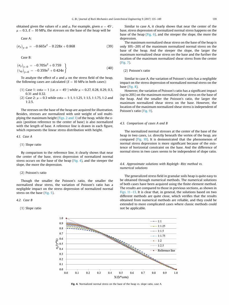
The stresses on the base of the heap are acquired for illustration.Besides, stresses are normalized with unit weight of soil multi-plying the maximum height (Figs. 2 and 3) of the heap, while the x-axis (position reference to the center of base) is also normalizedwith the length of base. A reference line is drawn in each figure,which represents the linear stress distribution with height.

4.1. Case A

(1) Slope ratio

By comparison to the reference line, it clearly shows that nearthe center of the base, stress depression of normalized normalstress occurs on the base of the heap (Fig. 4), and the steeper theslope, the more the depression.

(2) Poisson’s ratio

Though the smaller the Poisson’s ratio, the smaller thenormalized shear stress, the variation of Poisson’s ratio has anegligible impact on the stress depression of normalized normalstress on the base (Fig. 5).

4.2. Case B

(1) Slope ratio

Fig. 4. Normalized normal stress on the ba

Similar to case A, it clearly shows that near the center of thebase, stress depression of normalized normal stress happens on thebase of the heap (Fig. 6), and the steeper the slope, the more thedepression.

Themaximumnormalized shear stress on the base of the heap isonly 10%e20% of the maximum normalized normal stress on thebase of the heap. And the steeper the slope, the larger themaximum normalized shear stress on the base and the further thelocation of the maximum normalized shear stress from the center(Fig. 7).

(2) Poisson’s ratio

Similar to case A, the variation of Poisson’s ratio has a negligibleimpact on the stress depression of normalized normal stress on thebase (Fig. 8).

However, the variation of Poisson’s ratio has a significant impact(up to 20%) on themaximum normalized shear stress on the base ofthe heap. And the smaller the Poisson’s ratio, the larger themaximum normalized shear stress on the base. However, thelocation of the maximum normalized shear stress is independent ofPoisson’s ratio (Fig. 9).

4.3. Comparison of cases A and B

The normalized normal stresses at the center of the base of theheap in two cases, i.e. directly beneath the vertex of the heap, arecompared (Fig. 10). It is demonstrated that the phenomenon ofnormal stress depression is more significant because of the exis-tence of horizontal constraint on the base. And the difference ofnormal stress in two cases seems to be independent of slope ratio.

4.4. Approximate solutions with RayleigheRitz method vs.numerical solutions

The generalized stress field in granular soils heap is quite easy tobe obtained through numerical methods. The numerical solutionsof both cases have been acquired using the finite element method.The results are compared to those in previous sections, as shown inFigs. 11e13. It is clear that, in general, the solutions based on twodifferent methods are quite close, which verifies that the resultsobtained from numerical methods are reliable, and they could beextended to more complicated cases where classic methods couldnot be applicable.

se of the heap vs. slope ratio, case A.

Fig. 5. Normalized normal stress on the base of the heap vs. Poisson’s ratio, case A.

Fig. 6. Normalized normal stress on the base of the heap vs. slope ratio, case B.

Fig. 7. Normalized shear stress on the base of the heap vs. slope ratio, case B.

G. Bi / Journal of Rock Mechanics and Geotechnical Engineering 9 (2017) 135e149140

5. Conclusions and suggestions

Stress field in granular soils heap (including piled coal) is usuallyacquired through measurements and numerical simulations.Because the former method is not reliable as pressure cellsinstrumented on the interface between piled coal and underlyingsoft soil are not working well, results from numerical methodsalone are necessary to be doubly checked with one more method

before they are extended to more complex cases. The generalizedstress field in granular soils heap is analyzed with RayleigheRitzmethod in this article. Several conclusions are drawn below:

(1) The problem is divided into two cases: case A without hori-zontal constraint on the base and case B with horizontalconstraint on the base. In either case, the displacementfunctions u(x, y) and v(x, y) are assumed to be cubic

Fig. 8. Normalized normal stress on the base of the heap vs. Poisson’s ratio, case B.

Fig. 9. Normalized shear stress on the base of the heap vs. Poisson’s ratio, case B.

G. Bi / Journal of Rock Mechanics and Geotechnical Engineering 9 (2017) 135e149 141

polynomials with twelve undetermined parameters, whichsatisfy the Cauchy’s partial differential equations, general-ized Hooke’s law and boundary equations.

(2) A function is built with the RayleigheRitz method, and theproblem is converted into solving two undetermined pa-rameters through the variation of the function to reach theminimum potential energy, while other parameters areexpressed in terms of these two parameters.

Fig. 10. Normalized normal stress at the center of the base.

(3) Stress depression (i.e. normalized normal stress less thanunit) happens near the center of the base in both cases, andthe steeper the slope, the more the depression, while thevariation of the Poisson’s ratio has a negligible impact on it.

(4) For case B, themaximumnormalized shear stress on the baseof the heap is only 10%e20% of the maximum value. Thesteeper the slope, the larger the maximum normalized shearstress on the base, and the further the location of themaximum normalized shear stress from the center. Thevariation of the Poisson’s ratio has a significant impact (up to20%) on the maximum normalized shear stress, i.e. thesmaller the Poisson’s ratio, the larger the maximumnormalized shear stress. However, the location of themaximum normalized shear stress is independent of Pois-son’s ratio.

(5) Comparison between cases A and B shows that the stressdepression directly beneath the vertex of the heap is moresignificant because of the horizontal constraint on the base,and the difference of the normal stress in two cases isessentially independent of slope ratio.

(6) The RayleigheRitz method is capable of studying thegeneralized stress field in granular soils heap, and the resultsobtained by the RayleigheRitz method and numerical sim-ulations are quite close, which verifies that the numericalsimulations are reliable to be extended to more complicatedcases where classic methods could not be applicable.

Fig. 11. Normalized normal stresses from two methods for case A.

Fig. 12. Normalized normal stresses from two methods for case B.

Fig. 13. Normalized shear stresses from two methods for case B.

G. Bi / Journal of Rock Mechanics and Geotechnical Engineering 9 (2017) 135e149142

Conflict of interest

The authors wish to confirm that there are no known conflicts ofinterest associated with this publication and there has been nosignificant financial support for this work that could have influ-enced its outcome.

Appendix

This section is presented with the software Mathcad (or Math-cad Prime).

(1) Variation of the function for case A

G. Bi / Journal of Rock Mechanics and Geotechnical Engineering 9 (2017) 135e149 143

Reorganizing the fifth equation in Eq. (3) following thedescending power of x, below are the coefficients of constant, x, andx2, from top to bottom:

temp1coeffs;x/

0@ a1 sinaþa6h

2 sinaþmb1 sinaþ2mb3hsinaþ3mb6h2 sina

2a2 sina�2a6hsinatana�2mb3 sinatana�6mb6hsinatanaþa6hcosaþb4hcosa�ma6hcosa�mb4hcosa3a4 sinaþa6 sinatan

2aþmb4 sinaþ3mb6sinatan2a�a6cosatana�b4cosatanaþma6cosatanaþmb4cosatana

1A

(A1)

Reorganizing the sixth equation in Eq. (3) following thedescending power of x, below are the coefficients of constant, x, andx2, from top to bottom:

temp2coeffs;x/

0@ b1cosaþ2b3hcosaþ3b6h

2cosaþma1cosaþma6h2cosa

�2b3cosatana�6b6hcosatanaþ2ma2cosa�2ma6hcosatanaþa6hsinaþb4hsina�ma6hsina�mb4hsinab4cosaþ3b6cosatan

2aþ3ma4cosaþma6cosatan2a�a6 sinatana�b4 sinatanaþma6 sinatanaþmb4 sinatana

1A

(A2)

The above coefficients (of constant, x, and x2) must be equal tozero, respectively.

For the coefficients of constant, sinacosa can be ignored, reor-ganizing equations following the descending power of Poisson’sratio m yields

eq1 :¼�

a1 þ a6h2

b1 þ 2b2hþ 3b6h2

�(A3)

eq2 :¼�b1 þ 2b3hþ 3a6h

2

a1 þ a6h2

�(A4)

Again the coefficients (of m) must be equal to zero, respectively.It is noticed that there are only four parameters (a4, b4, a6 and b6)

in the coefficients of x2. The results of coefficients of m, a6 and b6 are

a4 : ¼ �13tan2 a cos a� tan3 a sin aþ 2m sin a tan a� cos aþ m co

cos a� sin a tan aþ m sin a tan aþ m

� m2 tan3 a sin a� m cos a tan2 aþ tan2 a cos a� m sin a tancos a� sin a tan aþ m sin a tan aþ m cos a� 2m2 cos a

chosen as the basic parameters, while other parameters (a1, a2, a3,b1, b3 and b4) are expressed in terms of a6 and b6.

According to the coefficient of m, the following expression can beobtained:

a1 :¼ �a6h2 (A5)

For the coefficient of x2, reorganizing equations following thepower of a4, b4, a6 and b6, respectively, yields

eq41 : ¼ 3a4 sin aþ a6�sin a tan2 a� sin aþ m sin a

�þ ð2m sin a� sin aÞb4 þ 3mb6 sin a tan2 a

(A6)

eq61 : ¼ b4ðcos a� sin a tan aþ m sin a tan aÞþ 3b6 cos a tan2 aþ 3ma4 cos aþ a6ð2m sin a tan a

� sin a tan aÞ(A7)

As mentioned before, the coefficient of x2 must be equal to zero,so, a4 and b4 are expressed in terms of a6 and b6:

s a� 3m2 sin a tan aþ m tan3 a sin a

cos a� 2m2 cos aa6

3 ab6

(A8)

G. Bi / Journal of Rock Mechanics and Geotechnical Engineering 9 (2017) 135e149144

b4 :¼�mcosaþm2cosaþmcosatan2aþsinatana�2msinatana

cosa�sinatanaþmsinatanaþmcosa�2m2cosaa6

þ �3tan2acosaþ3m2cosatan2a

cosa�sinatanaþmsinatanaþmcosa�2m2cosab6

(A9)

For the coefficient of x, there are five parameters (a2, a6, b3, b4and b6), while b4 has already been expressed in terms of a6 and b6.

In the same way, a2 and b3 are expressed in terms of a6 and b6:

a2 : ¼ 12h�2m2 sin2 aþ 5m sin2 a� 2 sin2 a tan2 aþ m2 cos2 aþ 2 sin2 aþ 2m2 tan2 a sin2 a� 5m3 sin2 a� cos2 a

2m sin a cos a� sin2 a tan aþ sin a cos aþ m2 tan a sin2 a� m2 tan a cos2 a� 2m3 tan a cos2 aa6

þ 12h

3m3 tan2 a sin2 a� 3m2 sin2 a� 3m tan2 a sin2 aþ 3 sin2 a

2m sin a cos a� sin2 a tan aþ sin a cos aþ m2 tan a sin2 a� m2 tan a cos2 a� 2m3 tan a cos2 ab6

(A10)

b3 : ¼�12sin2 a cos a� 1

2m2 tan a cos3 a� 1

2m cos3 aþ 1

2m3 cos3 a

�h

ð � 2m cos aþ sin a tan a� cos aÞsin a�m2 sin a� sin a

�a6þ�� 3 sin2 a cos a� 3

2m2 tan a sin3 a� 9

2m cos a sin2 a� 9

2m3 tan2 a cos3 aþ 3

2tan a sin3 aþ 3m2 cos a sin2 a

�

$h

ð � 2m cos aþ sin a tan a� cos aÞsin a�m2 sin a� sin a

�b6(A11)

According to the coefficient of m, b1 is expressed in terms of b3and b6:

b1 :¼ �2b3h� 3b6h2 (A12)

In this case, eight parameters are simplified into twoparameters.

To simplify the expressions of a1, a2, a4, b1, b3 and b4, C1eC12 aredefined. It should be noted that the expressions of C1eC12 are onlyrelated to a and m (i.e. having nothing to do with x and y):

a1 :¼ C1a6; b1 :¼ C7a6 þ C8b6 (A13)

a2 :¼ C3a6 þ C4b6; b3 :¼ C9a6 þ C10b6 (A14)

a4 :¼ C5a6 þ C6b6; b4 :¼ C11a6 þ C12b6 (A15)

The variation of the function is separated into four parts to bereadily calculated:

(i) Part 1

part1 :¼ 12sxεx (A16)

dda6

part1 :¼ C15a6 þ C16b6 (A17)

C15 : ¼ E1� m2

hC1 þ y2 þ C3xþ xðC3 þ 2C5xÞ þ C5x

2

þ m�C7 þ C11x

2 þ 2C9y�ih

C1 þ C5x2 þ y2 þ C3x

þ xðC3 þ 2C5xÞi (A18)

C16 : ¼12

E1�m2

nmhC12x

2þC8þC10yþyðC10þ2yÞþy2i

þxC4þxðC4þ2C6xÞþx2C6oh

C1þC5x2þy2þC3x

þxðC3þ2C5xÞiþ12

E1�m2

hC1þy2þC3xþxðC3þ2C5xÞ

þC5x2þm

�C7þC11x

2þ2C9y�ih

xC4þxðC4þ2C6xÞþx2C6i

(A19)

ddb6

part1 :¼ C17a6 þ C18b6 (A20)

C17 : ¼12

E1�m2

nmhC12x

2þC8þC10yþyðC10þ2yÞþy2i

þxC4þxðC4þ2xC6Þþx2C6oh

C1þC5x2þy2þC3x

þxðC3þ2xC5Þiþ12

E1�m2

hC1þy2þC3xþxðC3þ2xC5Þ

þC5x2þm

�C7þC11x

2þ2C9y�ih

xC4þxðC4þ2C6xÞþx2C6i

(A21)

C18 : ¼E

1�m2

nmhC12x

2þC8þC10yþyðC10þ2yÞþy2i

þxC4þxðC4þ2C6xÞþx2C6oh

xC4þxðC4þ2C6xÞþx2C6i

(A22)

(ii) Part 2

Part2 :¼ 12syεy (A23)

dda6

part2 :¼ C19a6 þ C20b6 (A24)

C19 : ¼ E1� m2

nC7 þ 2C9yþ C11x

2 þ mhC1 þ C5x

2 þ y2

þ C3xþ xðC3 þ 2C5xÞio�

C7 þ C11x2 þ 2C9y

� (A25)

G. Bi / Journal of Rock Mechanics and Geotechnical Engineering 9 (2017) 135e149 145

C20 : ¼12

E1�m2

nC12x

2þC8þC10yþ yðC10þ2yÞ

þmhxC4þ xðC4þ2C6xÞþ x2C6

iþy2

o�C7þC11x

2þ2C9y�

þ12

E1�m2

nC7þ2C9yþC11x

2þmhC1þC5x

2þ y2

þC3xþ xðC3þ2C5xÞioh

C12x2þC8þC10y

þyðC10þ2yÞþ y2i

(A26)

ddb6

part2 :¼ C21a6 þ C22b6 (A27)

C21 : ¼12

E1� m2

nC12x

2 þ C8 þ C10yþ yðC10 þ 2yÞ

þ mhxC4 þ xðC4 þ 2C6xÞ þ x2C6

iþ y2

o�C7 þ C11x

2 þ 2C9y�

þ 12

E1� m2

nC7 þ 2C9yþ C11x

2 þ mhC1 þ C5x

2 þ y2 þ C3x

þ xðC3 þ 2C5xÞioh

C12x2 þ C8 þ C10yþ yðC10 þ 2yÞ þ y2

i(A28)

C22 : ¼E

2

nC12x

2þC8þC10yþyðC10þ2yÞ

1�m

þmhxC4þxðC4þ2C6xÞþx2C6

iþy2

ohC12x

2þC8

þC10yþyðC10þ2yÞþy2i (A29)

(iii) Part 3

part3 :¼ 12sxygxy (A30)

dda6

part3 :¼ C23a6 þ C24b6 (A31)

C23 :¼ E1þ m

ðxyþ yC11xÞ2 (A32)

C24 :¼ 2E

1þ myC12xðxyþ yC11xÞ (A33)

temp1 coeffs;x/

0BBBBBBBBBBBBBB@

mb1 sinaþa1h sinaþa3h2 s

12a1 cosa�2a3h sina tana�ma3h cosa�

þ2a2h sina�2mb3 sina tana�mb

12a2 cosa�2a2 sina tanaþa3 sina tana�a3 cos

�b4 cosa tanaþ3mb

ddb6

part3 ¼ C25a6 þ C26b6 (A34)

C25 :¼ 2E

1þ myC12xðxyþ yC11xÞ (A35)

C26 :¼ 2E

1þ my2C2

12x2 (A36)

(iv) Part 4

part4 :¼ �gV (A37)

dda6

part4 :¼ C27 (A38)

C27 :¼ �gy�C9yþ C7 þ C11x

2�

(A39)

ddb6

part4 :¼ C28 (A40)

C28 :¼ �gy�C12x

2 þ C8 þ C10yþ y2�

(A41)

Adding four parts will yield the following two equations:

eq3 :¼ ðC15 þ C19 þ C23Þa6 þ ðC16 þ C20 þ C24Þb6 þ C27(A42)

eq4 :¼ ðC17þC21þC25Þa6þðC18þC22þC26Þb6þC28 (A43)

According to the principle of minimum potential energy, Eqs.(A42) and (A43) should be equal to zero, respectively. So, the ex-pressions of a6 and b6 can be obtained in terms of a and m, whileC15eC28 need to be integrated with respect to the heap.

(2) Variation of the function for case B

Reorganizing the fifth equation in Eq. (4) following thedescending power of x, below are the coefficients of constant, x, andx2, from top to bottom:

inaþ3mb6h2 sinaþ2mb3h sina

12ma1 cosa�a1 sina tanaþa3h cosa

4h cosaþb4h cosa�6mb6h sina tana

a tanaþma3 cosa tana�12ma2 cosaþmb4 cosa tana

6 sina tan2 aþmb4 sina

1CCCCCCCCCCCCCCA

(A44)

G. Bi / Journal of Rock Mechanics and Geotechnical Engineering 9 (2017) 135e149146

Reorganizing the sixth equation in Eq. (3) following thedescending power of x, below are the coefficients of constant, x, andx2, from top to bottom:

temp2 coeffs; x/

0BBBBBBBBBBBBBB@

2b3h cos aþ 3b6h2 cos aþ b1 cos aþ ma1h cos aþ ma3h

2 cos a

�12ma1 sin a� mb4h sin a� b4h sin aþ 2ma2h cos aþ 1

2a1 sin a� 6b6h cos a tan a� 2b3 cos a tan a

�ma1 cos a tan a� 2ma3h cos a tan a� ma3h sin aþ a3h sin a

12a2 sin aþ b4 cos a� 1

2ma2 sin aþ ma3 sin a tan a� b4 sin a tan aþ mb4 sin a tan aþ ma3 cos a tan2 a

�2ma2 cos a tan aþ 3b6 cos a tan2 a� a3 sin a tan a

1CCCCCCCCCCCCCCA

(A45)

The above coefficients (of constant, x, and x2) must be equal tozero, respectively.

For the coefficients of constant, sinacosa can be ignored, reor-ganizing equations following the descending power of Poisson’sratio m:

eq1 :¼�

a1hþ a3h2

b1 þ 2b3hþ 3b6h2

�(A46)

eq2 :¼�b1 þ 2b3hþ 3b6h

2

a1hþ a3h2

�(A47)

C3 : ¼�� 6m2 sin a tan aþ 2m cos aþ 4m sin a tan a� 2 sin a tan3 a� 2 cos a

þ 2m sin a tan3 aþ 2 cos a tan2 a� sin a

5 sin2 aþ 4m sin2 tan2 a� 4 sin2 tan2 aþ m cos2 a� 9m2 sin2 aþ 5m sin2 a� 1

(A51)

C4 : ¼�6m2 sin a tan3 a� 6m sin a tan a� 6m sin a tan3 a

þ 6 sin a tan a� sin a

5 sin2 aþ 4m sin2 a tan2 a� 4 sin2 a tan2 aþ m cos2 a� 9m2 sin2 aþ 5m sin2 a� 1

(A52)

Again the coefficients (of m) must be equal to zero, respectively.It is noticed that there are only four parameters (a2, b4, a3 and b6)

in the coefficients of x2, the results of coefficients of m, a3 and b6 arechosen as the basic parameters, while the other parameters (a1, a2,b1, b3 and b4) are expressed in terms of a3 and b6.

For the coefficient of x2, reorganizing equations following thepower of a2, b4, a3 and b6, respectively, yields

eq41 : ¼�� 2 sin a tan aþ 1

2cos a� 1

2m cos a

�a2

þ�sin a tan2 a� sin aþ m sin a

�a3

þ ð � sin aþ 2m sin aÞb4 þ 3mb6 sin a tan2 a

(A48)

eq61 : ¼��52m sinaþ1

2sina

�a2

þð� sina tanaþ2m sina tanaÞa3þðcosa� sina tanaþm sina tanaÞb4þ3b6 sina tana

(A49)

As mentioned before, the coefficient of x2 must be equal to zero,so, a2 and b4 are expressed in terms of a3 and b6:

a2 :¼ C3a3 þ C4b6 (A50)

b4 :¼ C9a3 þ C10b6 (A53)

C9 :¼ sin a�9m sin aþ 3 sin a tan2 a� 3m sin a tan2 aþ 3m2 sin a� 2 sin a

5 sin2 aþ 4m sin2 a tan2 a� 4 sin2 a tan2 aþ m cos2 a� 9m2 sin2 aþ 5m sin2 a� 1(A54)

C10 :¼ sin a�12 sin a tan2 aþ 3 sin aþ 15m2 sin a tan2 a� 3m sin a tan2 a� 3m sin a

5 sin2 aþ 4m sin2 a tan2 a� 4 sin2 a tan2 aþ m cos2 a� 9m2 sin2 aþ 5m sin2 a� 1(A55)

G. Bi / Journal of Rock Mechanics and Geotechnical Engineering 9 (2017) 135e149 147

For the coefficient of x, there are five parameters (a1, a2, a3, b3and b4), while a1, a2 and a4 have already been expressed in terms ofa3 and b6.

In the same way, b3 is expressed in terms of a6 and b6:

b3 :¼ C7a3 þ C8b6 (A56)

C7 :¼ h�C9m cos2 a tanaþC9 sin

2 a tana�mC3 cos2 aþC3 sin2 a�

3m sin2 a�cos2 aþ2sin2 a�tana

(A57)

C8 :¼ h3 cos2 a tan a� mC10 cos2 a tan aþ C4 sin2 a� 6 sin2 a tan a� mC4 cos2 a� 9m sin2 a tan aþ C10 sin2 a tan a�

3m sin2 a� cos2 aþ 2 sin2 a�tan a

(A58)

In this case, eight parameters are simplified into twoparameters.

To simplify the expressions of a1, a2, a3, b3 and b4, C1eC12 aredefined. It should be noted that C1eC12 are expressions only relatedto a and m (i.e. having nothing to do with x and y).

The variation of the function is separated into four parts to bereadily calculated:

(i) Part 1

part1 :¼ 12sxεx (A59)

dda3

part1 :¼ C15a3 þ C16b6 (A60)

C15 :¼ E1� m2

hyðC1 þ C3xþ yÞ þ xyC3 þ m

�C5 þ C9x

2 þ 2C7y�i

$½yðC1 þ C3xþ yÞ þ xyC3� (A61)

C16 : ¼�12

E1� m2

n2xyC4 þ m

hC6 þ C8yþ C10x

2 þ y2

þ yðC8 þ 2yÞio

½yðC1 þ C3xþ yÞ þ xyC3�

þ E1� m2

hyðC1 þ C3xþ yÞ þ xyC3

þ m�C5 þ C9x

2 þ 2C7y�xyC4

i(A62)

ddb6

part1 :¼ C17a3 þ C18b6 (A63)

C17 : ¼�12

E2

n2xyC4 þ m

hC6 þ C8yþ C10x

2 þ y2

1� m

þ yðC8 þ 2yÞio

½yðC1 þ C3xþ yÞ þ xyC3�

þ E1� m2

hyðC1 þ C3xþ yÞ þ xyC3

þ m�C5 þ C9x

2 þ 2C7y�i

xyC4

(A64)

C18 :¼2E

1�m2

n2xyC4þm

hC6þC8yþC10x

2þy2þyðC8þ2yÞio

xyC4

(A65)

(ii) Part 2

part2 :¼ 12syεy (A66)

dda3

part2 :¼ C19a3 þ C20b6 (A67)

C19 : ¼ E1� m2

nC5 þ C9x

2 þ 2C7yþ m½yðC1 þ C3xþ yÞ þ xyC3�o

$�C5 þ C9x

2 þ 2C7y�

(A68)

C20 : ¼ 12

E1� m2

hC6 þ C8yþ C10x

2 þ y2 þ yðC8 þ 2yÞ þ 2mxyC4i

$�C5 þ C9x

2 þ 2C7y�þ 12

E1� m2

nC5 þ C9x

2 þ 2C7y

þ m½yðC1 þ C3xþ yÞ þ xyC3�oh

C6 þ C8yþ C10x2 þ y2

þ yðC8 þ 2yÞi

(A69)

G. Bi / Journal of Rock Mechanics and Geotechnical Engineering 9 (2017) 135e149148

ddb6

part2 :¼ C21a3 þ C22b6 (A70)

C21 : ¼12

E1�m2

hC6þC8yþC10x

2þy2þyðC8þ2yÞ

þ2mxyC4i�

C5þC9x2þ2C7y

�þ12

E1�m2

$nC5þC9x

2þ2C7yþm½yðC1þC3xþyÞþxyC3�o

$hC6þC8yþC10x

2þy2þyðC8þ2yÞi

(A71)

C22 : ¼E

1�m2

hC6þC8yþC10x

2þy2þyðC8þ2yÞ

þ2mxyC4ihC6þC8yþC10x

2þy2þyðC8þ2yÞi (A72)

(iii) Part 3

part3 :¼ 12sxygxy (A73)

dda3

part3 :¼ C23a3 þ C24b6 (A74)

C23 :¼ E2ð1þ mÞ½xðC1 þ C3xþ yÞ þ xyþ 2C9xy�2 (A75)

C24 :¼ E2ð1þ mÞ

�x2C4 þ 2yC10x

�½xðC1 þ C3xþ yÞ þ xyþ 2C9xy�

(A76)

ddb6

part3 :¼ C25a3 þ C26b6 (A77)

C25 :¼ E2ð1þ mÞ

�x2C4 þ 2yC10x

�½xðC1 þ C3xþ yÞ þ xyþ 2C9xy�

(A78)

C26 :¼ E2ð1þ mÞ

�x2C4 þ 2xyC10

�2(A79)

(iv) Part 4

part4 :¼ �gV (A80)

dda3

part4 :¼ C27 (A81)

C27 :¼ �gy�C7yþ C5 þ C9x

2�

(A82)

ddb6

part4 :¼ C28 (A83)

C28 :¼ �gy�C10x

2 þ C6 þ C8yþ y2�

(A84)

Adding four parts will yield the following two equations:

eq3 :¼ ðC15 þ C19 þ C23Þa3 þðC16 þ C20 þ C24Þb6 þ C27 (A85)

eq4 :¼ ðC17 þ C21 þ C25Þa3 þðC18 þ C22 þ C26Þb6 þ C28 (A86)

According to the principle of minimum potential energy, thetwo equations should be equal to zero, respectively. So, the ex-pressions of a3 and b6 can be yielded in terms of a and m, while C15eC28 need to be integrated with respect to the heap.

References

Ai J, Ooi JY, Chen JF, Rotter JM, Zhong Z. The role of deposition process on pressuredip formation underneath a granular pile. Mechanics of Materials 2013;66:160e71.

Angelillo M, Babilio E, Fortunato A, Lippiello M, Montanino A. Analytic solutionsfor the stress field in static sandpiles. Mechanics of Materials 2016;95:192e203.

Bi G, Wei JF, Zhou L. Study of depression of stress on base of sand prism based onfixed principal axes assumption. Rock and Soil Mechanics 2014;35(4):1141e6(in Chinese).

Bi G, Wei JF, Niu HM, Jiang JX. Numerical study on the distribution of embankmentdeposit contact stress. Science Technology and Engineering 2016;16(27):255e9(in Chinese).

Bishop AW. Progressive failure with special reference to the mechanism causing it.In: Proceedings of the geotechnical conference, vol. 2. Norway, Oslo: NorwegianGeotechnical Institute; 1967. p. 142e50.

Bouchaud JP, Cates ME, Claudin P. Stress distribution in granular media andnonlinear wave equation. Journal de Physique I 1995;5(6):639e56.

Cates ME, Wittmer JP, Bouchaud JP, Claudin P. Development of stresses in cohe-sionless poured sand. Philosophical Transactions of the Royal Society A1998;356(1747):2535e60.

Cox GM. Stress distributions beneath heaps and rat-hole problems for granularmaterials [PhD Thesis]. University of Wollongong; 2001.

Da Silva M, Rajchenbach J. Stress transmission through a model system of cohe-sionless elastic grains. Nature 2000;406(6797):708e10.

Edwards SF, Grinev DV. The statistical-mechanical theory of stress transmission ingranular materials. Physica A: Statistical Mechanics and Its Applications1999;263(1):545e53.

Herrmann HJ, Hovi JP, Luding S. Physics of dry granular media. Springer Science &Business Media; 2013.

Hill JM, Cox GM. The force distribution at the base of sand-piles. In: Smith DW,Carter JP, editors. Development in theoretical geomechanics, proceedings of thebooker memorial symposium. Rotterdam: A.A. Balkema; 2000. p. 43e61.

Hill JM, Cox GM. On the problem of the determination of force distributions ingranular heaps using continuum theory. The Quarterly Journal of Mechanicsand Applied Mathematics 2002;55(4):655e68.

Jaky J. The coefficient of earth pressure at rest. Journal of the Society of HungarianArchitects and Engineers 1944;7:355e8 (in Hungarian).

Krimer DO, Pfitzner M, Bräuer K, Jiang Y, Liu M. Granular elasticity: generalconsiderations and the stress dip in sand piles. Physical Review E 2006;74.061310.

Liffman K, Nguyen M, Cleary P. Stress in sandpiles. In: Proceedings of the 2nd In-ternational conference on CFD in the minerals and process industries; 1999.p. 83e7.

Matuttis HG, Schinner A. Influence of the geometry on the pressure distribution ofgranular heaps. Granular Matter 1999;1(4):195e201.

Matuttis HG, Luding S, Herrmann HJ. Discrete element simulations of dense pack-ings and heaps made of spherical and non-spherical particles. Powder Tech-nology 2000;109(1e3):278e92.

Michalowski RL, Park N. Admissible stress fields and arching in piles of sand.Geotechnique 2004;54(8):529e38.

Michalowski RL, ParkN.Arching ingranular soils. In:Geomechanics: testing,modeling,and simulation. American Society of Civil Engineers (ASCE); 2005. p. 255e68.

Osterberg JO. Influence values for vertical stresses in semi-infinite mass due toembankment loading. In: Proceedings of the 4th International conference onsoil mechanics and foundation engineering, vol. 1; 1957. p. 393e6.

Pipatpongsa T, Matsushita T, Tanaka M, Kanazawa S, Kawai K. Theoretical andexperimental studies of stress distribution in wedge-shaped granular heaps.Acta Mechanica Solida Sinica 2014;27(1):28e40.

Savage SB. Problems in the statics and dynamics of granular materials. In:Behringer RP, Jenkins JT, editors. Powders and grains 97. Rotterdam: A.A. Ral-kema; 1997. p. 185e94.

Sokolovskii VV. Statics of granular media. Elsevier; 2013.

G. Bi / Journal of Rock Mechanics and Geotechnical Engineering 9 (2017) 135e149 149

Vanel L, Howell D, Clark D, Behringer RP, Clément E. Memories in sand: experi-mental tests of construction history on stress distributions under sandpiles.Physical Review E 1999;60:R5040e3.

Vanel L, Claudin P, Bouchaud JP, Cates ME, Clément E, Wittmer JP. Stresses in silos:comparison between theoretical models and new experiments. Physical ReviewLetters 2000;84(7):1439e42.

Watson A. Searching for the sand-pile pressure dip. Science 1996;273(5275):579e80.

Zheng Q, Yu A. Why have continuum theories previously failed to describe sandpileformation? Physical Review Letters 2014;113(6). 068001.

Zhu J, Liang Y, Zhou Y. The effect of the particle aspect ratio on the pressure at thebottom of sandpiles. Powder Technology 2013;234:37e45.