Embed Size (px)
Citation preview
Journal of Public Economics 93 (2009) 246–263
Contents lists available at ScienceDirect
Journal of Public Economics
j ourna l homepage: www.e lsev ie r.com/ locate /econbase
Born on the first of July: An (un)natural experiment in birth timing☆
Joshua S. Gans a,⁎, Andrew Leigh b
a Melbourne Business School, University of Melbourne, Australiab Research School of Social Sciences, Australian National University, Australia
a r t i c l e i n f o
☆ In part, this paper uses confidentialised unit recordwas initiated and is funded by the Australian DepartmMelbourne Institute of Applied Economic and Social Rshould not be attributed to either FaHCSIA or the MIAEStern, Justin Wolfers, seminar participants at Columbrecent births data than a previous version, though thi⁎ Corresponding author.
E-mail addresses: [email protected] (J.S. GanURL's: http://www.mbs.edu/jgans (J.S. Gans), http
0047-2727/$ – see front matter © 2008 Elsevier B.V.doi:10.1016/j.jpubeco.2008.07.004
a b s t r a c t
Article history:Received 6 June 2007Received in revised form 3 June 2008Accepted 21 July 2008Available online 24 July 2008
It is well understood that government policies can distort behavior. But what is less oftenrecognized is that the anticipated introduction of a policy can introduce its own distortions. Westudy one such “introduction effect,” using evidence from a unique policy change in Australia. In2004, the Australian government announced that children born on or after July 1, 2004 wouldreceive a $3000 “Baby Bonus.” Although the policy was only announced sevenweeks before itsintroduction, parents appear to have behaved strategically in order to receive the benefit, withthe number of births dipping sharply before the policy commenced. On July 1, 2004, moreAustralian children were born than on any other single date in the past thirty years. Weestimate that over 1000 births were “moved” so as to ensure that their parents were eligible forthe Baby Bonus, with about one quarter being moved bymore than one week. Most of the effectwas due to changes in the timing of induction and cesarean section procedures. We findevidence to suggest that babies who were shifted into the eligibility period were more likely tobe of high birth weight. Two years later, on July 1, 2006, the Baby Bonus was increased, and wefind that this again caused births to be moved from June to July. These birth timing eventsrepresent an opportunity for health researchers to study the impact of planned birthdays andhospital management issues.
© 2008 Elsevier B.V. All rights reserved.
JEL classification:H31J13
Keywords:Introduction effectTiming of birthsPolicy distortion
TIM LESTER: Minister, with the benefit of hindsight, would it have been better to have announced and introduced this policy onthe same day?
KAY PATTERSON: This policy is a bonus to families. TIM LESTER: That doesn't answer my question, though, with respect, Minister. Would it have been better to have announced andintroduced this policy at the same time? KAY PATTERSON: I believe this is a fantastic policy for mothers, they're going to get $3000 –file data from the Household, Income and Labour Dynamics in Australia (HILDA) survey. The HILDA Projecent of Families, Housing, Community Services and Indigenous Affairs (FaHCSIA) and is managed by theesearch (MIAESR). The findings and views reported in this paper, however, are those of the authors andSR. We are grateful to Heather Booth, Bruce Chapman, Paul Frijters, Joe Hirschberg, Susanne Schmidt, Scotia University and two anonymous referees for valuable comments on earlier drafts. This paper uses mores has only a slight impact on the results.
s), [email protected] (A. Leigh).://econrsss.anu.edu.au/~aleigh/ (A. Leigh).
All rights reserved.
t
t
1 From2 Exc
the US,3 All4 Prec5 Incl6 In t7 The8 Mill
commeannoun
247J.S. Gans, A. Leigh / Journal of Public Economics 93 (2009) 246–263
TIM LESTER: Minister, that still doesn't answer my question with respect. Would it have been better to have announced andintroduced this policy at the same time?
KAY PATTERSON: Well if I thought that mothers would put their babies at risk, but I don't believe mothers would put them at risk.11. Introduction
Economists have long been concerned that seemingly subtle issues of policy announcements and the timing of policy shifts canhave dramatic short-term effects on individual behavior. Consider a situationwhere a government announces a new tax benefit ora subsidy that will be introduced at some later date. It can be expected that – to the extent that they have some discretion as to thetiming of their decisions – individuals will shift their actions around the policy introduction date to take advantage of a benefit oravoid a detriment. Just as the existence of government policies can distort behavior, so too policy changes can further distortindividuals' decisions. Such an effect might be termed an introduction effect.
Frequently, the announcement that a new tax or subsidy will take effect upon a certain date leads to news reports of individualsor firms rearranging their affairs so as to take advantage of the policy change. However, it is rare to find an opportunity inwhich theeffect of such policy changes can be quantitatively estimated.2
In this paper, we identify a policy change that created the potential for an introduction effect. On May 11, 2004, the Australiangovernment announced that it would give a $3000 Maternity Payment, commonly referred to as a ‘Baby Bonus’ to each family of anewborn child.3 For our purposes, the important feature of the Baby Bonus policywas that it was to only apply for babies born on orafter July 1, 2004. Thus, a household with a child born at 11:59 pm on June 30, 2004, would receive no payment while one with achild born at 12:01 am on July 1, 2004, and thereafter would receive $3000.4 This creates the potential for an introduction effectespecially given the lag between the policy announcement and the introduction date.
The seven week lag between the policy announcement and its introduction would not have an impact on the number ofpregnancies as those affected by the introduction were already in the process; the third trimester, in fact.5 However, it could havean impact on either (i) discretionary and planned birth timing decisions (such as inductions and elective cesarians) and/or (ii) thereporting of birthdays. In each case, the impact on reported birth timing would be jointly determined by the parents and doctorinvolved.6
We obtained daily data on all recorded births in Australia from 1975 to 2004. Even without any statistical analysis, the effectappears dramatic. On June 30, 2004 (a Wednesday), 500 babies were registered as having been born, a birthrate at the 11thpercentile of the births distribution over the entire period 1975–2004 (and the 1st percentile of the births distribution onweekdays).7 On July 1, 2004, 1005 babies were born. This was the highest number of births recorded throughout the 10,958-dayperiod 1975–2004. The fifth-highest number of births on a single day was July 2, 2004 with 928.
With a flexible functional form, allowing for separate day-of-year, day-of-week and year effects, we find that the introduction ofthe Baby Bonus was associated with a substantial increase in the birth rate. Our results are highly statistically significant, as well asbeing economically significant. Over the window covering 28 days before and 28 days after the policy was introduced, we estimatethat over 1000 births were moved into the eligibility range. Data from induction and cesarean section procedures indicate thatthese accounted for most of the shift. Analyzing a subsample of birth records, we find that babies born in early-July weresignificantly heavier than those born in late-June, which would be consistent with parents delaying births to obtain the payment.All of this provides an indication that shifting was, in fact, real and not a result of reporting issues or fraud.
As well as providing an experiment that identifies an introduction effect, our result here is also a contribution to ourunderstanding of the short-run drivers of the timing of births. Chandra et al. (2004) demonstrated that birth numbers fall onweekends as compared with weekdays, and that this effect has grown over time. They also found that less risky births were morelikely to be moved. A very similar trend away fromweekend births has also occurred in Australia (Gans and Leigh, 2007). Indeed, aswe discuss below, it is important that we take account of day-of-week effects when estimating the true magnitude of theintroduction effect.
In relation to the impact of government policies, Dickert-Conlin and Chandra (1999) demonstrated that tax incentives in the UScaused births to be shifted from the first week of January each year to the last week of December. They estimated that increasingthe tax benefit of having a child by $500 raised the probability of an end of December birth by 26.9%.8 Our paper offers a distinctinsight into birth timing and incentives. First, the government policy created an incentive to delay the birth as opposed to bringingit forward. As babies are often born prematurely, there is intrinsically less control in this decision than a decision for an earlier birth.
the 7:30 Report (ABC Television, July 1, 2004); Kay Patterson was the Minister for Health in the Australian Government.eptions to this are Kopczuk and Slemrod (2003), Gans and Leigh (2006a), and Eliason and Ohlsson (2008), who find that changes in the estate tax rate inAustralia, and Sweden had an impact on the number of reported deaths.figures are in Australian dollars. In 2004, A$1=US$0.75 (approx).isely 12:00 am was apparently a ‘grey’ area (Sunday Telegraph, June 27, 2004, p.5).uding the third child of the first author; eventually born on July 25, 2004.he case of home births, it would be the mid-wife. However, we do not separately identify these in our data.re were some births reported close to midnight: ABC Radio (July 1, 2004) reported a birth at 11:53pm.igan (2005) studied the introduction of a ‘baby bonus’ (or Allowance for Newborn Children) in Quebec, Canada. However, in that case, the policynced on the day of its announcement, so there was no potential for an introduction effect. In 2006, the German and Singaporean governments bothced that they planned to offer payments to new parents, potentially creating the opportunity for further investigation of introduction effects.
248 J.S. Gans, A. Leigh / Journal of Public Economics 93 (2009) 246–263
Second, the US tax incentive exists in every year, allowing hospitals to allocate additional resources to take account of it. Theintroduction of the Baby Bonus in Australia had a one-off effect, and so likely created unplanned resource utilization problems. Inthis situation, one would expect hospitals and doctors to have been more constrained in their ability to respond to parentalrequests to adjust the timing of the birth so that they were eligible for the Baby Bonus. Our observed impacts are, therefore,informative as to the degree of power that patients have over the timing of births.9
While the Australian Baby Bonus represents a clean experiment in analyzing the introduction effect, there is some questionwhether what mattered was an increase in real incentives provided by the Baby Bonus or a reaction to a clearer and moretransparent set of incentives. As we describe below, the Baby Bonus replaced an earlier child birth incentive. In contrast to the newBaby Bonus, however, this earlier benefit was income-related and so varied considerably depending on individual circumstance.Also, it was a benefit realized with some considerable delay whereas the Baby Bonus cash payment was immediate.10 Given itsrelative complexity, it is unclear whether the earlier policy was recognized as an incentive at all.11
The paper proceeds as follows. In the next section, we describe in more detail the Australian Baby Bonus and its predecessor.Section 3 estimates the total number of births that were moved. Section 4 decomposes the effect across birth procedures. Section 5analyzes the characteristics of those babies that were born, and their parents. Section 6 presents the results of a subsequentincrease in the Baby Bonus, which occurred in 2006. The final section concludes.
2. The Australian Baby Bonus
From July 1, 2004, the Baby Bonus operated very simply. If a family gave birth to a child after this date, they automaticallyreceived a cash payment of $3000. The payment was untaxed, and was given to all parents regardless of income. For the medianhousehold, this amount was worth 5.4% of annual disposable income (equivalent to 2.8 weeks' post-tax income).12 The paymentwas per baby and so for the multiple births the payment was $6000 for twins or $9000 for triplets.
The policy was announced as part of the 2004–2005 Budget. It was not anticipated and can, therefore, be taken as essentiallyunknown prior toMay 11, 2004.13 The stated goal of the policy was “to provide further help at the crucial period around the birth ofa child” (Australian Treasury, 2004, 33) (though with Australian voters due to go to the polls in late-2004, purely political motivescannot be ruled out; particularly as the Opposition Leader had proposed a similar policy in March 2004). There was considerablepublicity about the introduction of the policy when it was announced, and further coverage in June 2004.14 This included a mediadiscussion as to whether the policy might encourage teenage pregnancy and suggestions that teenagers might in future beexcluded from receiving the bonus.15
The Baby Bonuswe described here replaced a previous policy, which operated as a refundable tax offset.16 That policyworked asfollows: for each baby born between July 1, 2001 and June 30, 2004, the primary carer of the child (that is, the parent staying athome) was eligible to claim for a bonus.17 The bonus depended on the income the primary carer earned in the tax year (in Australiafrom July to June) that the child was born. If the primary carer's incomewas $25,000 or less, the taxpayer would receive $500/yr.18
If the income exceeded this amount, then the taxpayer would only receive a payment if their income fell. In this case, the benefitcould potentially be quite large. The size of the payment depended on the taxpayer's income level prior to having a baby (Inc0),their average tax rate in that year (τ0), and their income level in year t (where t≤5). The yearly bonus in year twas then calculatedas follows:19
9 As Ccase for10 The11 Agabenefit12 Aut13 A mprobabl14 Fordad, annewspa15 Onparentslump suand tha16 Thechange,17 Bot18 The19 Theincome
Yearly Bonust ¼ 1−InctInc0
� �min τ0Inc0; D12;500ð Þ
5
handra et al. (2004) noted, it is unclear whether the weekend/public holiday decline is driven by doctor/hospital or patient preferences. This is not thechanges in timing based on the Baby Bonus.first author received his $3000 payment via electronic transfer in 5 weeks.in the first author's experience is instructive here. Prior to the introduction of the new Baby Bonus, his household was blissfully unaware of any financiato having a child.hors' calculations, based on the Household, Income and Labour Dynamics in Australia survey (HILDA).edia search in the weeks prior to the budget reveals that the government made it known to some journalists in early May that the Baby Bonus wouldy be revamped in the budget. However, details were not provided at the time, so the changes remained speculative.example, much coverage was given to the Treasurer's suggestion to the media on May 11, 2004 that Australian parents should have “one for mom, one ford one for the country.”. A search of the Factiva database for the terms “Baby Bonus” and “Maternity Payment” returns 411 articles published in Australianpers during May and June 2004.the furor over teens, see for example Arndt (2004), Grattan and Nguyen (2004). On 1 January 2007, the Australian government changed the rules so thaaged 17 years or under would receive the Baby Bonus in 13 fortnightly installments, unless special circumstances existed to warrant the payment of am. On 15 May 2008, the government announced that all families would receive the Baby Bonus in 13 fortnightly installments (commencing 1 July 2008)t eligibility would be restricted to families with adjusted taxable income equivalent to $150,000 or less a year (commencing 1 January 2009).new Baby Bonus also replaced the Maternity Allowance, a means-tested payment to those families receiving Family Tax Benefit A. At the time of thethe Maternity Allowance was worth $842.64 per child for eligible families.h the old Baby Bonus and the new Baby Bonus were also available to adoptive parents.first year amount would be reduced to take into account the birth date of the child.re were adjustments to this based on part-years for the beginning and end of the first 5 years. The amount was payable following the lodgment of antax return with a minimum time to refund of 3 to 15 months depending upon when in the year the child was born.
l
t
,
20 As Lduring pThese w21 Sincmakes itwo pro22 Of cto sugg23 Relaaccepta
249J.S. Gans, A. Leigh / Journal of Public Economics 93 (2009) 246–263
us, carers earning high salaries (in particular, those paying a lot of tax) just prior to having a baby and then earning very little
Ththereafter would receive the maximum payment of $2500/yr.20 The new Baby Bonus announced in 2004 was anticipated to beconsiderably more expensive to the government than the previous scheme. In its last year of operation (tax year 2003–04),expenditures on the old child payment were $150million (ATO, 2004, 368).21 In its first year of operation, the new Baby Bonus wasexpected to cost the federal government $741 million (Australian Treasury, 2004, 37).22Nonetheless, there may exist households for which there were incentives to time births prior to July 1, 2004 rather than on orafter that date (as they would receive potentially 5 years of benefits from the old policy). For other households, the differencebetween the old payment and the new paymentmay have been less than $3000. To the extent that this is the case, any introductioneffect from the new Baby Bonus will understate the impact of a $3000 financial incentive on birth timing.23
3. Baby Bump?
With changes in medical technology and practice, doctors and patients have increased discretion over the timing of births.At dates prior to when a natural, vaginal delivery of a child would occur, births can be induced or brought about by cesareansection. The ‘safe’ window of discretion is potentially greater than three weeks. For example, guidelines defined by theAmerican Academy of Pediatrics and the American College of Obstetricians and Gynecologists define pre-term births as thosethat occur up to the end of the 37th week of pregnancy, term births as those that occur from the 38th to the 42nd week, andpost-term births as those that occur on or after the first day of the 43rd week of pregnancy (AAP, ACOG, 2002; see also WHO,1992; Engle, 2006).
While medical and health concerns play an important role in any exercise in discretion over birth timing, there is evidence thatnon-medical issues also play a role. There is a long-term trend towards fewer births on weekends (Chandra et al., 2004; Gans andLeigh, 2007) and even reductions in birth rates on auspicious days (Lo, 2003; Gans and Leigh, 2006b, in press) and during the weekof the annual conference of professional obstetrics associations (Gans et al., 2007). In addition, in Australia and the United States,there is a mini-baby boom each year 7–10 days prior to Christmas Day perhaps reflective of joint preferences of doctors andpatients not to have births at that time (Gans et al., 2007). Consequently, it is plausible that direct financial incentives may affectbirth timing.
The introduction of the Baby Bonus gave parents an incentive not to schedule births prior to July 1. As a consequence, it isplausible that some births that would have otherwise been expected to occur prior to that date did not. Moreover, it is likely thatthe incentives and the degree of discretion to change scheduled procedures in response to the Baby Bonus introduction effectwould be stronger closer to July 1, 2004. Consequently, this will have an impact on the mix of birth delivery mechanisms observedprior and after that date.
To test the impact of the Baby Bonus on recorded births, we use daily data on the number of Australian births. There aretwo main sources of births data — figures collected by state and territory births registries, compiled by the Australian Bureauof Statistics (ABS); and data collected from hospitals, compiled by the Australian Institute of Health and Welfare (AIHW).Each source has its limitations: unregistered births do not appear in the ABS data, while home births do not appear in theAIHW data. By using both data sources, we hope to circumvent the problems that would arise from only analyzing one or theother.
Since the ABS births data cover a longer time span, our central analysis uses these data. They include all recorded births from1975–2004. While the birth rate in Australia has declined over this period, the number of births has remained relatively constant(there were 232,682 births in 1975, and 245,143 births in 2004). We therefore opt to focus on the number of births, rather than onthe birth rate. This has the added advantage that we do not introduce noise into our series through mis-measurement of the totalpopulation, which is only available on a monthly basis.
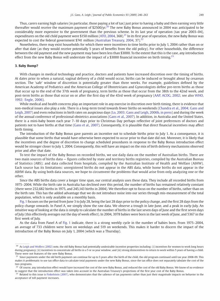
Fig.1 focuses on the period from June 3 to July 28, being the last 28 days prior to the policy change, and the first 28 days from thepolicy change onwards. In Panel A, we simply show the raw data. We observe a trough in late-June, and a peak in early-July. Anintuitiveway of looking at the data is simply to calculate the number of births in the last seven days of June and the first seven daysof July (this effectively averages out the day of week effect). In 2004, 3978 babies were born in the last week of June, and 5367 in thefirst week of July.
As the data from Panel A of Fig. 1 indicate, there is a strong weekly cycle in the number of babies born. From 1975–2004,an average of 733 children were born on weekdays and 519 on weekends. This makes it harder to discern the impact of theintroduction of the Baby Bonus on July 1, 2004 (which was a Thursday).
eigh andWolfers (2002) note, the old Baby Bonus had potentially undesirable incentive properties including: (i) incentives for women to work long hoursregnancy; (ii) incentives to concentrate all births in a 5 or so year window; and (iii) strong disincentives to return to work within 5 years of having a child.ere not features of the new Baby Bonus.e payments under the old birth payment can continue for up to 5 years after the birth of the child, the old program continued until tax year 2008-09. Thist problematic to use tax office data to calculate total payments under the new Baby Bonus, since the tax office does not separately tabulate the cost of thegrams.ourse, any introduction effect would have increased the cost of the new Baby Bonus, and reduced the cost of the old Baby Bonus. We know of no evidenceest that the introduction effect was taken into account in the Australian Treasury's projections of the first year cost of the Baby Bonus.ted to this issue is Finkelstein (2007), who demonstrates that the salience of tax payments rather than just their magnitude impacts on behavior in thence of toll payment increases.
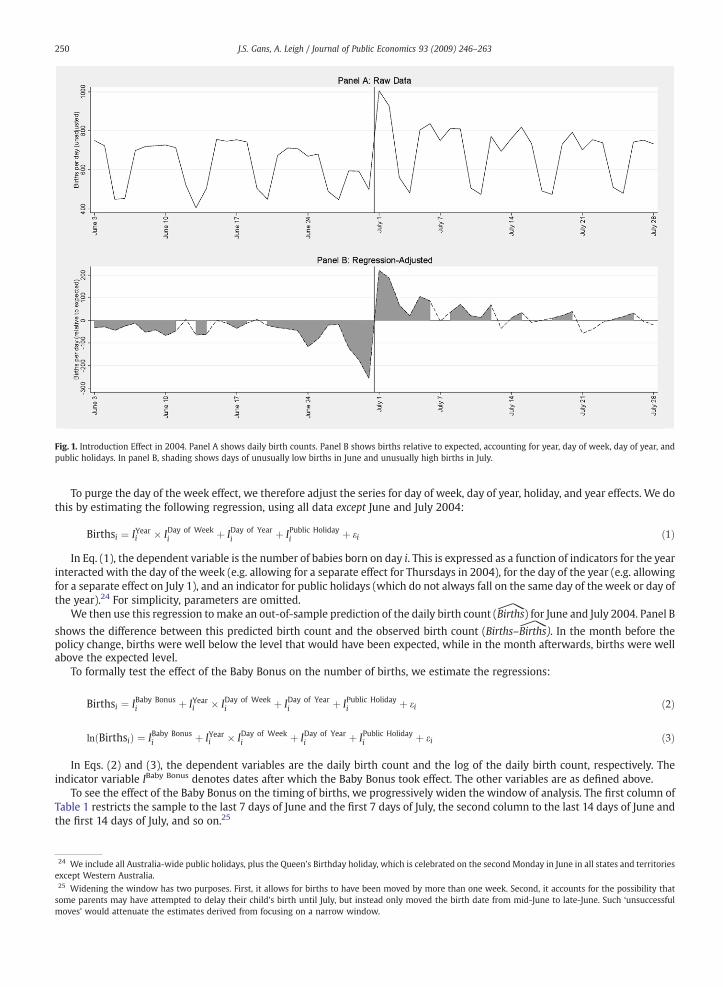
Fig. 1. Introduction Effect in 2004. Panel A shows daily birth counts. Panel B shows births relative to expected, accounting for year, day of week, day of year, andpublic holidays. In panel B, shading shows days of unusually low births in June and unusually high births in July.
24 We include all Australia-wide public holidays, plus the Queen's Birthday holiday, which is celebrated on the second Monday in June in all states and territoriesexcept Western Australia.25 Widening the window has two purposes. First, it allows for births to have been moved by more than one week. Second, it accounts for the possibility thasome parents may have attempted to delay their child's birth until July, but instead only moved the birth date from mid-June to late-June. Such ‘unsuccessfumoves’ would attenuate the estimates derived from focusing on a narrow window.
250 J.S. Gans, A. Leigh / Journal of Public Economics 93 (2009) 246–263
To purge the day of the week effect, we therefore adjust the series for day of week, day of year, holiday, and year effects. We dothis by estimating the following regression, using all data except June and July 2004:
Birthsi ¼ IYeari � IDay of Weeki þ IDay of Year
i þ IPublic Holidayi þ ei ð1Þ
Eq. (1), the dependent variable is the number of babies born on day i. This is expressed as a function of indicators for the year
Ininteracted with the day of the week (e.g. allowing for a separate effect for Thursdays in 2004), for the day of the year (e.g. allowingfor a separate effect on July 1), and an indicator for public holidays (which do not always fall on the same day of the week or day ofthe year).24 For simplicity, parameters are omitted.We then use this regression to make an out-of-sample prediction of the daily birth count (1Births) for June and July 2004. Panel B
shows the difference between this predicted birth count and the observed birth count (Births–1Births). In the month before the
policy change, births were well below the level that would have been expected, while in the month afterwards, births were wellabove the expected level.
To formally test the effect of the Baby Bonus on the number of births, we estimate the regressions:
Birthsi ¼ IBaby Bonusi þ IYeari � IDay of Week
i þ IDay of Yeari þ IPublic Holiday
i þ ei ð2Þ
ln Birthsið Þ ¼ IBaby Bonusi þ IYeari � IDay of Week
i þ IDay of Yeari þ IPublic Holiday
i þ ei ð3Þ
Eqs. (2) and (3), the dependent variables are the daily birth count and the log of the daily birth count, respectively. The
Inindicator variable IBaby Bonus denotes dates after which the Baby Bonus took effect. The other variables are as defined above.To see the effect of the Baby Bonus on the timing of births, we progressively widen the window of analysis. The first column ofTable 1 restricts the sample to the last 7 days of June and the first 7 days of July, the second column to the last 14 days of June andthe first 14 days of July, and so on.25
tl
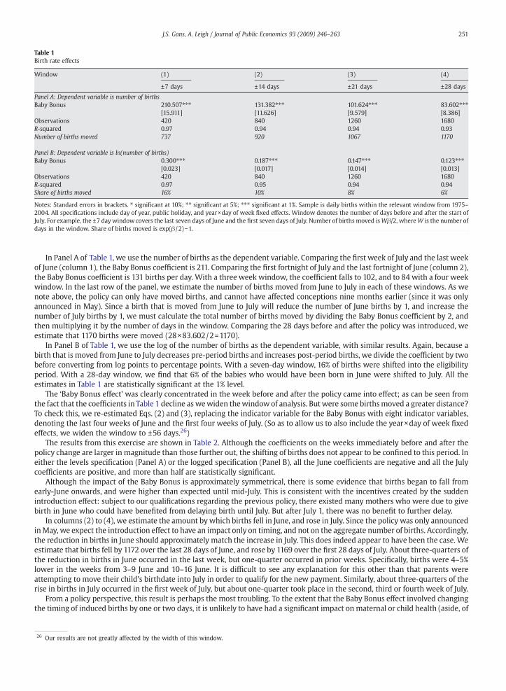
Table 1Birth rate effects
Window (1) (2) (3) (4)
±7 days ±14 days ±21 days ±28 days
Panel A: Dependent variable is number of birthsBaby Bonus 210.507⁎⁎⁎ 131.382⁎⁎⁎ 101.624⁎⁎⁎ 83.602⁎⁎⁎
[15.911] [11.626] [9.579] [8.386]Observations 420 840 1260 1680R-squared 0.97 0.94 0.94 0.93Number of births moved 737 920 1067 1170
Panel B: Dependent variable is ln(number of births)Baby Bonus 0.300⁎⁎⁎ 0.187⁎⁎⁎ 0.147⁎⁎⁎ 0.123⁎⁎⁎
[0.023] [0.017] [0.014] [0.013]Observations 420 840 1260 1680R-squared 0.97 0.95 0.94 0.94Share of births moved 16% 10% 8% 6%
Notes: Standard errors in brackets. ⁎ significant at 10%; ⁎⁎ significant at 5%; ⁎⁎⁎ significant at 1%. Sample is daily births within the relevant window from 1975–2004. All specifications include day of year, public holiday, and year×day of week fixed effects. Window denotes the number of days before and after the start oJuly. For example, the ±7 day window covers the last seven days of June and the first seven days of July. Number of births moved isWβ/2, whereW is the number odays in the window. Share of births moved is exp(β /2)−1.
26 Our results are not greatly affected by the width of this window.
251J.S. Gans, A. Leigh / Journal of Public Economics 93 (2009) 246–263
ff
In Panel A of Table 1, we use the number of births as the dependent variable. Comparing the first week of July and the last weekof June (column 1), the Baby Bonus coefficient is 211. Comparing the first fortnight of July and the last fortnight of June (column 2),the Baby Bonus coefficient is 131 births per day. With a three week window, the coefficient falls to 102, and to 84 with a four weekwindow. In the last row of the panel, we estimate the number of births moved from June to July in each of these windows. As wenote above, the policy can only have moved births, and cannot have affected conceptions nine months earlier (since it was onlyannounced in May). Since a birth that is moved from June to July will reduce the number of June births by 1, and increase thenumber of July births by 1, we must calculate the total number of births moved by dividing the Baby Bonus coefficient by 2, andthen multiplying it by the number of days in the window. Comparing the 28 days before and after the policy was introduced, weestimate that 1170 births were moved (28×83.602/2=1170).
In Panel B of Table 1, we use the log of the number of births as the dependent variable, with similar results. Again, because abirth that is moved from June to July decreases pre-period births and increases post-period births, we divide the coefficient by twobefore converting from log points to percentage points. With a seven-day window, 16% of births were shifted into the eligibilityperiod. With a 28-day window, we find that 6% of the babies who would have been born in June were shifted to July. All theestimates in Table 1 are statistically significant at the 1% level.
The ‘Baby Bonus effect’ was clearly concentrated in the week before and after the policy came into effect; as can be seen fromthe fact that the coefficients in Table 1 decline aswewiden thewindow of analysis. But were some birthsmoved a greater distance?To check this, we re-estimated Eqs. (2) and (3), replacing the indicator variable for the Baby Bonus with eight indicator variables,denoting the last four weeks of June and the first four weeks of July. (So as to allow us to also include the year×day of week fixedeffects, we widen the window to ±56 days.26)
The results from this exercise are shown in Table 2. Although the coefficients on the weeks immediately before and after thepolicy change are larger in magnitude than those further out, the shifting of births does not appear to be confined to this period. Ineither the levels specification (Panel A) or the logged specification (Panel B), all the June coefficients are negative and all the Julycoefficients are positive, and more than half are statistically significant.
Although the impact of the Baby Bonus is approximately symmetrical, there is some evidence that births began to fall fromearly-June onwards, and were higher than expected until mid-July. This is consistent with the incentives created by the suddenintroduction effect: subject to our qualifications regarding the previous policy, there existed many mothers who were due to givebirth in June who could have benefited from delaying birth until July. But after July 1, there was no benefit to further delay.
In columns (2) to (4), we estimate the amount bywhich births fell in June, and rose in July. Since the policy was only announcedinMay, we expect the introduction effect to have an impact only on timing, and not on the aggregate number of births. Accordingly,the reduction in births in June should approximately match the increase in July. This does indeed appear to have been the case. Weestimate that births fell by 1172 over the last 28 days of June, and rose by 1169 over the first 28 days of July. About three-quarters ofthe reduction in births in June occurred in the last week, but one-quarter occurred in prior weeks. Specifically, births were 4–5%lower in the weeks from 3–9 June and 10–16 June. It is difficult to see any explanation for this other than that parents wereattempting to move their child's birthdate into July in order to qualify for the new payment. Similarly, about three-quarters of therise in births in July occurred in the first week of July, but about one-quarter took place in the second, third or fourth week of July.
From a policy perspective, this result is perhaps the most troubling. To the extent that the Baby Bonus effect involved changingthe timing of induced births by one or two days, it is unlikely to have had a significant impact on maternal or child health (aside, of
27 At the extreme, it is possible that all the births that were shifted from 3-9 June were born in 10-16 June; that all the births that were shifted from 10-16 Junewere born in 17-23 June; and that all the births that were shifted from 17-23 June were born in 24-30 June.
Table 2Birth rate effects–medium run
(1) (2) (3) (4)
Total births moved
±14 days ±21 days ±28 days
Panel A: Dependent variable is number of birthsBefore
June 3–9, 2004 −22.036⁎[11.908]
June 10–16, 2004 −26.830⁎⁎[11.908] −1172
June 17–23, 2004 −15.884 −1017[11.905] −830
June 24–30, 2004 −102.632⁎⁎⁎[11.905]
AfterJuly 1–7, 2004 107.875⁎⁎⁎
[11.905]July 8–14, 2004 36.373⁎⁎⁎
[11.905] 1169July 15–21, 2004 15.353 1117
[11.905] 829July 22–28, 2004 7.427
[11.905]Observations 3360R-squared 0.94
Panel B: Dependent variable is ln(number of births)Before
June 3–9, 2004 −0.035⁎[0.018]
June 10–16, 2004 −0.046⁎⁎[0.018]
June 17–23, 2004 −0.022[0.018]
June 24–30, 2004 −0.158⁎⁎⁎[0.018]
AfterJuly 1–7, 2004 0.142⁎⁎⁎
[0.018]July 8–14, 2004 0.052⁎⁎⁎
[0.018]July 15–21, 2004 0.022
[0.018]July 22–28, 2004 0.016
[0.018]Observations 3360R-squared 0.94
Notes: Standard errors in brackets. ⁎ significant at 10%; ⁎⁎ significant at 5%; ⁎⁎⁎ significant at 1%. All specifications include day of year, public holiday, and year×dayof week fixed effects. Sample covers May 6 to August 25 (56 days before and 56 days after July 1) from 1975–2004. Total births moved is the sum of the coefficients(in weeks 1–2, 1–3 or 1–4), multiplied by 7.
252 J.S. Gans, A. Leigh / Journal of Public Economics 93 (2009) 246–263
course, from any consequences from unexpected congestion issues in maternity wards). But the results in Table 2 are consistentwith births being shifted by more than a few days. If all births that were shifted successfully qualified for the new payment, thenour results suggest that the introduction of the Baby Bonus led 300 births to be shiftedmore than 7 days, and over 150 to bemovedby more than 14 days. However, another possibility is that no large-scale shifting occurred, but that many parents tried and failedto qualify for the Baby Bonus.27 With aggregate data, we cannot separate these two hypotheses.
Nonetheless, the fact that the disruption caused by the Baby Bonus was not confined to a few days around July 1 is cause forsome concern, notwithstanding that the health consequences of shifting births are uncertain.
In addition, our methodology cannot tell us precisely the cause of the shift. One possibility is that moving births from late Juneto the first week of Julymay also have created congestion for that week. In that case, some births would have been pushed later into
28 Further evidence against the mis-reporting hypothesis is the birth weight data presented in Section 5.
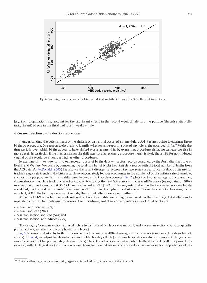
Fig. 2. Comparing two sources of birth data. Note: dots show daily birth counts for 2004. The solid line is at x=y.
253J.S. Gans, A. Leigh / Journal of Public Economics 93 (2009) 246–263
July. Such propagation may account for the significant effects in the second week of July, and the positive (though statisticallyinsignificant) effects in the third and fourth weeks of July.
4. Cesarean section and induction procedures
In understanding the determinants of the shifting of births that occurred in June–July, 2004, it is instructive to examine thosebirths by procedure. One reason to do this is to identify whether mis-reporting played any role in the observed shifts.28 While thetime periods over which births appear to have shifted works against this, by examining procedure shifts, we can explore this inmore detail. In particular, if themechanism for the shift was not discretionary procedure then it is likely that shifts for non-inducedvaginal births would be at least as high as other procedures.
To examine this, we now turn to our second source of births data — hospital records compiled by the Australian Institute ofHealth andWelfare. We begin by comparing the total number of births from this data source with the total number of births fromthe ABS data. As McDonald (2005) has shown, the recent divergence between the two series raises concerns about their use fortracking aggregate trends in the birth rate. However, our study focuses on changes in the number of births within a short window,and for this purpose we find little difference between the two data sources. Fig. 2 plots the two series against one another,demonstrating that they track one another closely. Regressing the raw ABS series on the raw AIHW series (using data for 2004)returns a beta coefficient of 0.9 (T=48.1) and a constant of 27.5 (T=2.0). This suggests that while the two series are very highlycorrelated, the hospital birth counts are on average 27 births per day higher than birth registrations data. In both the series, birthson July 1, 2004 (the first day on which the Baby Bonus took effect) are a clear outlier.
While the AIHW series has the disadvantage that it is not available over a long time span, it has the advantage that it allows us toseparate births into four delivery procedures. The procedures, and their corresponding share of 2004 births are:
• vaginal, not induced (50%);• vaginal, induced (20%);• cesarean section, induced (5%); and• cesarean section, not induced (25%).
(The category ‘cesarean section, induced’ refers to births in which labor was induced, and a cesarean section was subsequentlyperformed — generally due to complications in labor.)
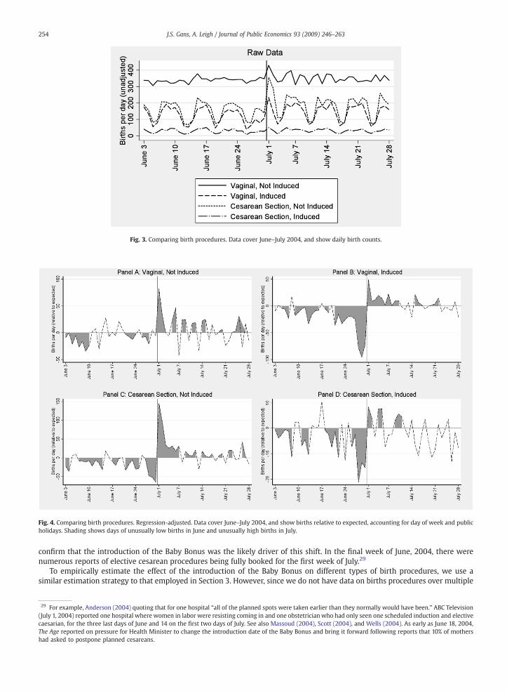
Fig. 3 decomposes births by birth procedure across June and July 2004, showing just the raw data (unadjusted for day-of-weekeffects). In Fig. 4, we adjust for day-of-week and public holiday effects (since our hospitals data do not span multiple years, wecannot also account for year and day-of-year effects). These two charts show that on July 1, births delivered by all four proceduresincrease, with the largest rise (in numerical terms) being for induced vaginal and non-induced cesarean section. Reported incidents
29 For example, Anderson (2004) quoting that for one hospital “all of the planned spots were taken earlier than they normally would have been.” ABC Television(July 1, 2004) reported one hospital where women in labor were resisting coming in and one obstetricianwho had only seen one scheduled induction and electivecaesarian, for the three last days of June and 14 on the first two days of July. See also Massoud (2004), Scott (2004), and Wells (2004). As early as June 18, 2004The Age reported on pressure for Health Minister to change the introduction date of the Baby Bonus and bring it forward following reports that 10% of mothershad asked to postpone planned cesareans.
Fig. 4. Comparing birth procedures. Regression-adjusted. Data cover June–July 2004, and show births relative to expected, accounting for day of week and publicholidays. Shading shows days of unusually low births in June and unusually high births in July.
Fig. 3. Comparing birth procedures. Data cover June–July 2004, and show daily birth counts.
254 J.S. Gans, A. Leigh / Journal of Public Economics 93 (2009) 246–263
confirm that the introduction of the Baby Bonus was the likely driver of this shift. In the final week of June, 2004, there werenumerous reports of elective cesarean procedures being fully booked for the first week of July.29
To empirically estimate the effect of the introduction of the Baby Bonus on different types of birth procedures, we use asimilar estimation strategy to that employed in Section 3. However, since we do not have data on births procedures over multiple
,
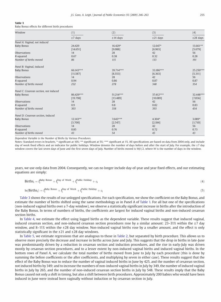
Table 3Baby Bonus effects for different birth procedures
Window (1) (2) (3) (4)
±7 days ±14 days ±21 days ±28 days
Panel A: Vaginal, not inducedBaby Bonus 24.429 16.429⁎ 12.647⁎ 13.661⁎⁎
[14.651] [9.088] [6.963] [5.679]Observations 14 28 42 56R-squared 0.67 0.38 0.32 0.28Number of births moved 86 115 133 191
Panel B: Vaginal, inducedBaby Bonus 66.143⁎⁎⁎ 39.714⁎⁎⁎ 33.186⁎⁎⁎ 25.250⁎⁎⁎
[11.587] [8.553] [6.363] [5.311]Observations 14 28 42 56R-squared 0.94 0.86 0.87 0.87Number of births moved 232 278 348 354
Panel C: Cesarean section, not inducedBaby Bonus 86.429⁎⁎⁎ 51.214⁎⁎⁎ 37.412⁎⁎⁎ 32.448⁎⁎⁎
[19.798] [13.489] [10.089] [7.856]Observations 14 28 42 56R-squared 0.9 0.8 0.82 0.83Number of births moved 303 358 393 454
Panel D: Cesarean section, inducedBaby Bonus 12.143⁎⁎ 7.643⁎⁎⁎ 4.304⁎ 3.089⁎
[3.700] [2.547] [2.184] [1.710]Observations 14 28 42 56R-squared 0.85 0.76 0.72 0.73Number of births moved 43 54 45 43
Dependent Variable is the Number of Births by Various Procedures.Notes: Standard errors in brackets. ⁎ significant at 10%; ⁎⁎ significant at 5%; ⁎⁎⁎ significant at 1%. All specifications are based on data from 2004 only, and includeday of week fixed effects and an indicator for public holidays. Window denotes the number of days before and after the start of July. For example, the ±7 daywindow covers the last seven days of June and the first seven days of July. Number of births moved is Wβ /2, where W is the number of days in the window.
255J.S. Gans, A. Leigh / Journal of Public Economics 93 (2009) 246–263
years, we use only data from 2004. Consequently, we can no longer include day-of-year and year fixed effects, and our estimatingequations are simply:
Birthsi ¼ IBaby Bonusi þ IDay of Week
i þ IPublic Holidayi þ ei ð4Þ
ln Birthsið Þ ¼ IBaby Bonusi þ IDay of Week
i þ IPublic Holidayi þ ei ð5Þ
le 3 shows the results of our unlogged specifications. For each specification, we show the coefficient on the Baby Bonus, and
Tabestimate the number of births shifted using the same methodology as in Panel A of Table 1. For all but one of the specifications(non-induced vaginal births over a 7-day window), we observe a statistically significant increase in births after the introduction ofthe Baby Bonus. In terms of numbers of births, the coefficients are largest for induced vaginal births and non-induced cesareansection births.In Table 4, we estimate the effect using logged births as the dependent variable. These results suggest that induced vaginal,induced cesarean section, and non-induced cesarean section procedures rose by a similar amount: 23–31% within the ±7 daywindow, and 8–11% within the ±28 day window. Non-induced vaginal births rose by a smaller amount, and the effect is onlystatistically significant in the ±21 and ±28 day windows.
In Table 5, we estimate regressions that are analogous to those in Table 2, but separated by birth procedure. This allows us toobserve more precisely the decrease and increase in births across June and July. This suggests that the drop in births in late-Junewas predominantly driven by a reduction in cesarean section and induction procedures, and the rise in early-July was drivenmostly by cesarean section procedures, and to a lesser extent by non-induced vaginal births and induced vaginal births. In thebottom rows of Panel A, we calculate the total number of births moved from June to July by each procedure (this is done bysumming the before coefficients or the after coefficients, and multiplying by seven in either case). These results suggest that theeffect of the Baby Bonus was to reduce the number of vaginal induced births in June by 425, and the number of cesarean section,not induced births by 349; and to increase the numbers of non-induced vaginal births in July by 349, the number of induced vaginalbirths in July by 265, and the number of non-induced cesarean section births in July by 548. These results imply that the BabyBonus caused not only a shift in timing, but also a shift between birth procedures. Approximately 200 babies whowould have beeninduced in June were instead born vaginally without induction or by cesarean section in July.
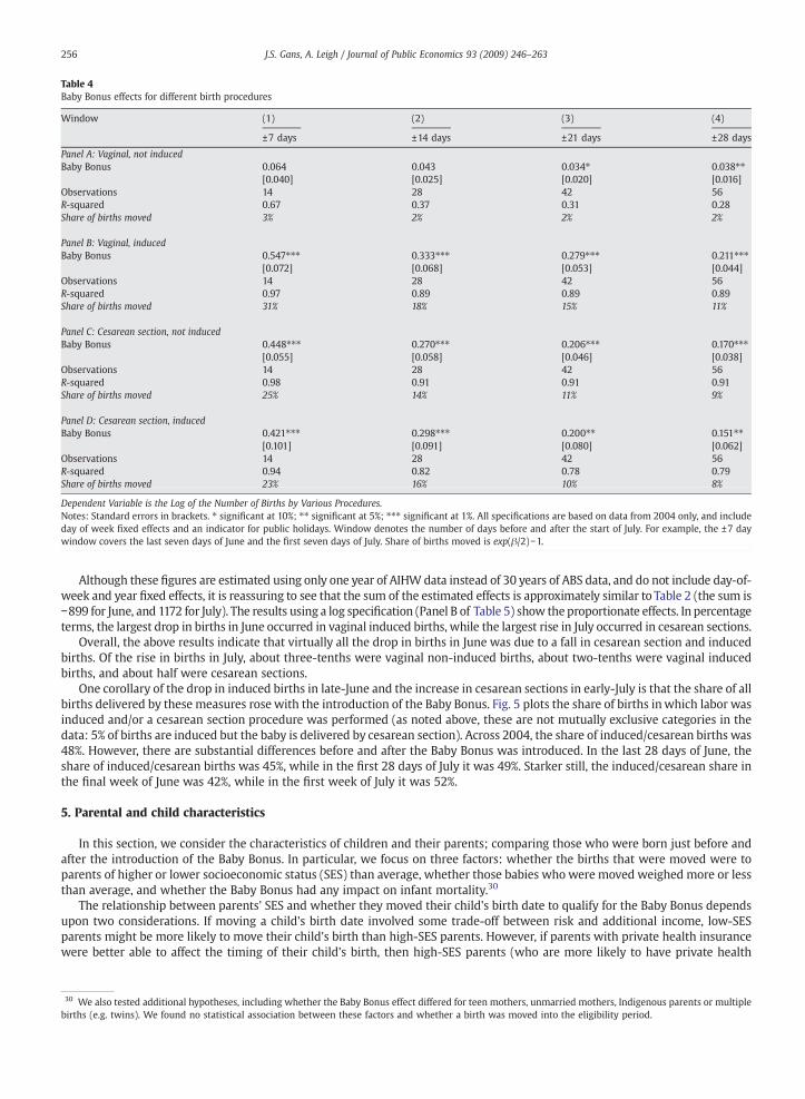
Table 4Baby Bonus effects for different birth procedures
Window (1) (2) (3) (4)
±7 days ±14 days ±21 days ±28 days
Panel A: Vaginal, not inducedBaby Bonus 0.064 0.043 0.034⁎ 0.038⁎⁎
[0.040] [0.025] [0.020] [0.016]Observations 14 28 42 56R-squared 0.67 0.37 0.31 0.28Share of births moved 3% 2% 2% 2%
Panel B: Vaginal, inducedBaby Bonus 0.547⁎⁎⁎ 0.333⁎⁎⁎ 0.279⁎⁎⁎ 0.211⁎⁎⁎
[0.072] [0.068] [0.053] [0.044]Observations 14 28 42 56R-squared 0.97 0.89 0.89 0.89Share of births moved 31% 18% 15% 11%
Panel C: Cesarean section, not inducedBaby Bonus 0.448⁎⁎⁎ 0.270⁎⁎⁎ 0.206⁎⁎⁎ 0.170⁎⁎⁎
[0.055] [0.058] [0.046] [0.038]Observations 14 28 42 56R-squared 0.98 0.91 0.91 0.91Share of births moved 25% 14% 11% 9%
Panel D: Cesarean section, inducedBaby Bonus 0.421⁎⁎⁎ 0.298⁎⁎⁎ 0.200⁎⁎ 0.151⁎⁎
[0.101] [0.091] [0.080] [0.062]Observations 14 28 42 56R-squared 0.94 0.82 0.78 0.79Share of births moved 23% 16% 10% 8%
Dependent Variable is the Log of the Number of Births by Various Procedures.Notes: Standard errors in brackets. ⁎ significant at 10%; ⁎⁎ significant at 5%; ⁎⁎⁎ significant at 1%. All specifications are based on data from 2004 only, and includeday of week fixed effects and an indicator for public holidays. Window denotes the number of days before and after the start of July. For example, the ±7 daywindow covers the last seven days of June and the first seven days of July. Share of births moved is exp(β/2)−1.
30 We also tested additional hypotheses, including whether the Baby Bonus effect differed for teen mothers, unmarried mothers, Indigenous parents or multiplebirths (e.g. twins). We found no statistical association between these factors and whether a birth was moved into the eligibility period.
256 J.S. Gans, A. Leigh / Journal of Public Economics 93 (2009) 246–263
Although these figures are estimated using only one year of AIHW data instead of 30 years of ABS data, and do not include day-of-week and year fixed effects, it is reassuring to see that the sum of the estimated effects is approximately similar to Table 2 (the sum is−899 for June, and 1172 for July). The results using a log specification (Panel B of Table 5) show the proportionate effects. In percentageterms, the largest drop in births in June occurred in vaginal induced births, while the largest rise in July occurred in cesarean sections.
Overall, the above results indicate that virtually all the drop in births in June was due to a fall in cesarean section and inducedbirths. Of the rise in births in July, about three-tenths were vaginal non-induced births, about two-tenths were vaginal inducedbirths, and about half were cesarean sections.
One corollary of the drop in induced births in late-June and the increase in cesarean sections in early-July is that the share of allbirths delivered by these measures rose with the introduction of the Baby Bonus. Fig. 5 plots the share of births inwhich labor wasinduced and/or a cesarean section procedure was performed (as noted above, these are not mutually exclusive categories in thedata: 5% of births are induced but the baby is delivered by cesarean section). Across 2004, the share of induced/cesarean births was48%. However, there are substantial differences before and after the Baby Bonus was introduced. In the last 28 days of June, theshare of induced/cesarean births was 45%, while in the first 28 days of July it was 49%. Starker still, the induced/cesarean share inthe final week of June was 42%, while in the first week of July it was 52%.
5. Parental and child characteristics
In this section, we consider the characteristics of children and their parents; comparing those who were born just before andafter the introduction of the Baby Bonus. In particular, we focus on three factors: whether the births that were moved were toparents of higher or lower socioeconomic status (SES) than average, whether those babies who were moved weighed more or lessthan average, and whether the Baby Bonus had any impact on infant mortality.30
The relationship between parents' SES and whether they moved their child's birth date to qualify for the Baby Bonus dependsupon two considerations. If moving a child's birth date involved some trade-off between risk and additional income, low-SESparents might be more likely to move their child's birth than high-SES parents. However, if parents with private health insurancewere better able to affect the timing of their child's birth, then high-SES parents (who are more likely to have private health
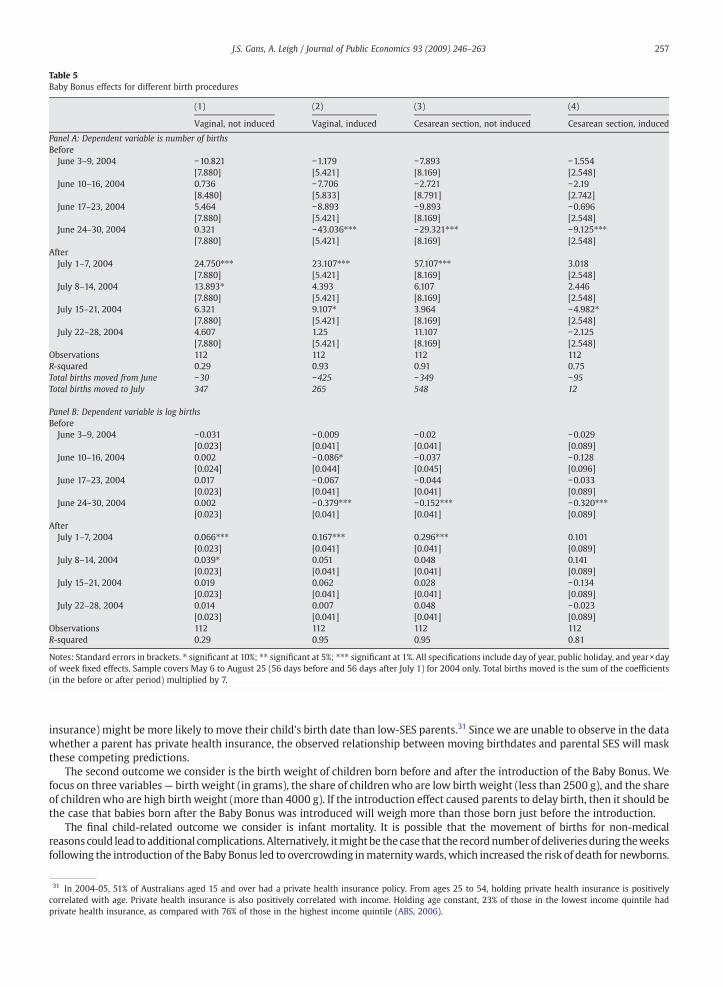
Table 5Baby Bonus effects for different birth procedures
(1) (2) (3) (4)
Vaginal, not induced Vaginal, induced Cesarean section, not induced Cesarean section, induced
Panel A: Dependent variable is number of birthsBeforeJune 3–9, 2004 −10.821 −1.179 −7.893 −1.554
[7.880] [5.421] [8.169] [2.548]June 10–16, 2004 0.736 −7.706 −2.721 −2.19
[8.480] [5.833] [8.791] [2.742]June 17–23, 2004 5.464 −8.893 −9.893 −0.696
[7.880] [5.421] [8.169] [2.548]June 24–30, 2004 0.321 −43.036⁎⁎⁎ −29.321⁎⁎⁎ −9.125⁎⁎⁎
[7.880] [5.421] [8.169] [2.548]AfterJuly 1–7, 2004 24.750⁎⁎⁎ 23.107⁎⁎⁎ 57.107⁎⁎⁎ 3.018
[7.880] [5.421] [8.169] [2.548]July 8–14, 2004 13.893⁎ 4.393 6.107 2.446
[7.880] [5.421] [8.169] [2.548]July 15–21, 2004 6.321 9.107⁎ 3.964 −4.982⁎
[7.880] [5.421] [8.169] [2.548]July 22–28, 2004 4.607 1.25 11.107 −2.125
[7.880] [5.421] [8.169] [2.548]Observations 112 112 112 112R-squared 0.29 0.93 0.91 0.75Total births moved from June −30 −425 −349 −95Total births moved to July 347 265 548 12
Panel B: Dependent variable is log birthsBeforeJune 3–9, 2004 −0.031 −0.009 −0.02 −0.029
[0.023] [0.041] [0.041] [0.089]June 10–16, 2004 0.002 −0.086⁎ −0.037 −0.128
[0.024] [0.044] [0.045] [0.096]June 17–23, 2004 0.017 −0.067 −0.044 −0.033
[0.023] [0.041] [0.041] [0.089]June 24–30, 2004 0.002 −0.379⁎⁎⁎ −0.152⁎⁎⁎ −0.320⁎⁎⁎
[0.023] [0.041] [0.041] [0.089]AfterJuly 1–7, 2004 0.066⁎⁎⁎ 0.167⁎⁎⁎ 0.296⁎⁎⁎ 0.101
[0.023] [0.041] [0.041] [0.089]July 8–14, 2004 0.039⁎ 0.051 0.048 0.141
[0.023] [0.041] [0.041] [0.089]July 15–21, 2004 0.019 0.062 0.028 −0.134
[0.023] [0.041] [0.041] [0.089]July 22–28, 2004 0.014 0.007 0.048 −0.023
[0.023] [0.041] [0.041] [0.089]Observations 112 112 112 112R-squared 0.29 0.95 0.95 0.81
Notes: Standard errors in brackets. ⁎ significant at 10%; ⁎⁎ significant at 5%; ⁎⁎⁎ significant at 1%. All specifications include day of year, public holiday, and year×dayof week fixed effects. Sample covers May 6 to August 25 (56 days before and 56 days after July 1) for 2004 only. Total births moved is the sum of the coefficient(in the before or after period) multiplied by 7.
31 In 2004-05, 51% of Australians aged 15 and over had a private health insurance policy. From ages 25 to 54, holding private health insurance is positivelycorrelated with age. Private health insurance is also positively correlated with income. Holding age constant, 23% of those in the lowest income quintile hadprivate health insurance, as compared with 76% of those in the highest income quintile (ABS, 2006).
257J.S. Gans, A. Leigh / Journal of Public Economics 93 (2009) 246–263
s
insurance) might be more likely to move their child's birth date than low-SES parents.31 Since we are unable to observe in the datawhether a parent has private health insurance, the observed relationship between moving birthdates and parental SES will maskthese competing predictions.
The second outcome we consider is the birth weight of children born before and after the introduction of the Baby Bonus. Wefocus on three variables— birth weight (in grams), the share of childrenwho are low birth weight (less than 2500 g), and the shareof childrenwho are high birth weight (more than 4000 g). If the introduction effect caused parents to delay birth, then it should bethe case that babies born after the Baby Bonus was introduced will weigh more than those born just before the introduction.
The final child-related outcome we consider is infant mortality. It is possible that the movement of births for non-medicalreasons could lead to additional complications. Alternatively, itmight be the case that the recordnumberof deliveriesduring theweeksfollowing the introduction of the Baby Bonus led to overcrowding inmaternitywards,which increased the risk of death for newborns.
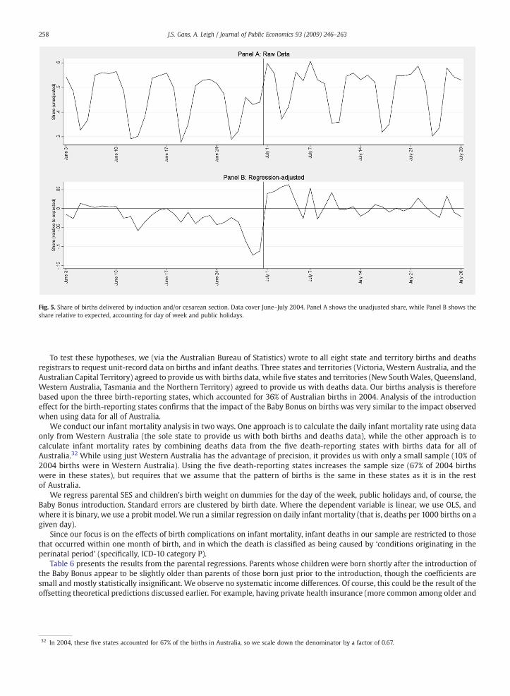
Fig. 5. Share of births delivered by induction and/or cesarean section. Data cover June–July 2004. Panel A shows the unadjusted share, while Panel B shows theshare relative to expected, accounting for day of week and public holidays.
32 In 2004, these five states accounted for 67% of the births in Australia, so we scale down the denominator by a factor of 0.67.
258 J.S. Gans, A. Leigh / Journal of Public Economics 93 (2009) 246–263
To test these hypotheses, we (via the Australian Bureau of Statistics) wrote to all eight state and territory births and deathsregistrars to request unit-record data on births and infant deaths. Three states and territories (Victoria, Western Australia, and theAustralian Capital Territory) agreed to provide us with births data, while five states and territories (New SouthWales, Queensland,Western Australia, Tasmania and the Northern Territory) agreed to provide us with deaths data. Our births analysis is thereforebased upon the three birth-reporting states, which accounted for 36% of Australian births in 2004. Analysis of the introductioneffect for the birth-reporting states confirms that the impact of the Baby Bonus on births was very similar to the impact observedwhen using data for all of Australia.
We conduct our infant mortality analysis in two ways. One approach is to calculate the daily infant mortality rate using dataonly from Western Australia (the sole state to provide us with both births and deaths data), while the other approach is tocalculate infant mortality rates by combining deaths data from the five death-reporting states with births data for all ofAustralia.32 While using just Western Australia has the advantage of precision, it provides us with only a small sample (10% of2004 births were in Western Australia). Using the five death-reporting states increases the sample size (67% of 2004 birthswere in these states), but requires that we assume that the pattern of births is the same in these states as it is in the restof Australia.
We regress parental SES and children's birth weight on dummies for the day of the week, public holidays and, of course, theBaby Bonus introduction. Standard errors are clustered by birth date. Where the dependent variable is linear, we use OLS, andwhere it is binary, we use a probit model. We run a similar regression on daily infant mortality (that is, deaths per 1000 births on agiven day).
Since our focus is on the effects of birth complications on infant mortality, infant deaths in our sample are restricted to thosethat occurred within one month of birth, and in which the death is classified as being caused by ‘conditions originating in theperinatal period’ (specifically, ICD-10 category P).
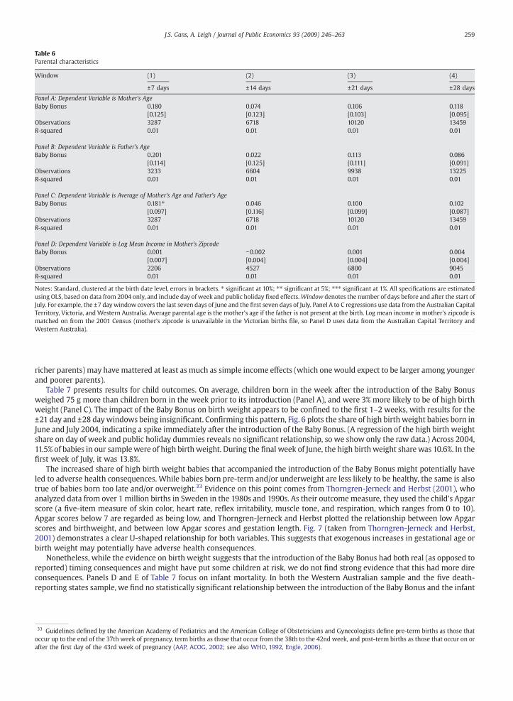
Table 6 presents the results from the parental regressions. Parents whose children were born shortly after the introduction ofthe Baby Bonus appear to be slightly older than parents of those born just prior to the introduction, though the coefficients aresmall and mostly statistically insignificant. We observe no systematic income differences. Of course, this could be the result of theoffsetting theoretical predictions discussed earlier. For example, having private health insurance (more common among older and
33 Guidelines defined by the American Academy of Pediatrics and the American College of Obstetricians and Gynecologists define pre-term births as those thaoccur up to the end of the 37th week of pregnancy, term births as those that occur from the 38th to the 42nd week, and post-term births as those that occur on oafter the first day of the 43rd week of pregnancy (AAP, ACOG, 2002; see also WHO, 1992, Engle, 2006).
Table 6Parental characteristics
Window (1) (2) (3) (4)
±7 days ±14 days ±21 days ±28 day
Panel A: Dependent Variable is Mother's AgeBaby Bonus 0.180 0.074 0.106 0.118
[0.125] [0.123] [0.103] [0.095]Observations 3287 6718 10120 13459R-squared 0.01 0.01 0.01 0.01
Panel B: Dependent Variable is Father's AgeBaby Bonus 0.201 0.022 0.113 0.086
[0.114] [0.125] [0.111] [0.091]Observations 3233 6604 9938 13225R-squared 0.01 0.01 0.01 0.01
Panel C: Dependent Variable is Average of Mother's Age and Father's AgeBaby Bonus 0.181⁎ 0.046 0.100 0.102
[0.097] [0.116] [0.099] [0.087]Observations 3287 6718 10120 13459R-squared 0.01 0.01 0.01 0.01
Panel D: Dependent Variable is Log Mean Income in Mother's ZipcodeBaby Bonus 0.001 −0.002 0.001 0.004
[0.007] [0.004] [0.004] [0.004]Observations 2206 4527 6800 9045R-squared 0.01 0.01 0.01 0.01
Notes: Standard, clustered at the birth date level, errors in brackets. ⁎ significant at 10%; ⁎⁎ significant at 5%; ⁎⁎⁎ significant at 1%. All specifications are estimatedusing OLS, based on data from 2004 only, and include day of week and public holiday fixed effects.Window denotes the number of days before and after the start oJuly. For example, the ±7 daywindow covers the last seven days of June and the first seven days of July. Panel A to C regressions use data from the Australian CapitaTerritory, Victoria, and Western Australia. Average parental age is the mother's age if the father is not present at the birth. Log mean income in mother's zipcode imatched on from the 2001 Census (mother's zipcode is unavailable in the Victorian births file, so Panel D uses data from the Australian Capital Territory andWestern Australia).
259J.S. Gans, A. Leigh / Journal of Public Economics 93 (2009) 246–263
s
fls
richer parents) may have mattered at least as much as simple income effects (which one would expect to be larger among youngerand poorer parents).
Table 7 presents results for child outcomes. On average, children born in the week after the introduction of the Baby Bonusweighed 75 g more than children born in the week prior to its introduction (Panel A), and were 3% more likely to be of high birthweight (Panel C). The impact of the Baby Bonus on birth weight appears to be confined to the first 1–2 weeks, with results for the±21 day and ±28 daywindows being insignificant. Confirming this pattern, Fig. 6 plots the share of high birth weight babies born inJune and July 2004, indicating a spike immediately after the introduction of the Baby Bonus. (A regression of the high birth weightshare on day of week and public holiday dummies reveals no significant relationship, so we show only the raw data.) Across 2004,11.5% of babies in our samplewere of high birth weight. During the final week of June, the high birth weight share was 10.6%. In thefirst week of July, it was 13.8%.
The increased share of high birth weight babies that accompanied the introduction of the Baby Bonus might potentially haveled to adverse health consequences. While babies born pre-term and/or underweight are less likely to be healthy, the same is alsotrue of babies born too late and/or overweight.33 Evidence on this point comes from Thorngren-Jerneck and Herbst (2001), whoanalyzed data from over 1 million births in Sweden in the 1980s and 1990s. As their outcomemeasure, they used the child's Apgarscore (a five-item measure of skin color, heart rate, reflex irritability, muscle tone, and respiration, which ranges from 0 to 10).Apgar scores below 7 are regarded as being low, and Thorngren-Jerneck and Herbst plotted the relationship between low Apgarscores and birthweight, and between low Apgar scores and gestation length. Fig. 7 (taken from Thorngren-Jerneck and Herbst,2001) demonstrates a clear U-shaped relationship for both variables. This suggests that exogenous increases in gestational age orbirth weight may potentially have adverse health consequences.
Nonetheless, while the evidence on birth weight suggests that the introduction of the Baby Bonus had both real (as opposed toreported) timing consequences and might have put some children at risk, we do not find strong evidence that this had more direconsequences. Panels D and E of Table 7 focus on infant mortality. In both the Western Australian sample and the five death-reporting states sample, we find no statistically significant relationship between the introduction of the Baby Bonus and the infant
tr
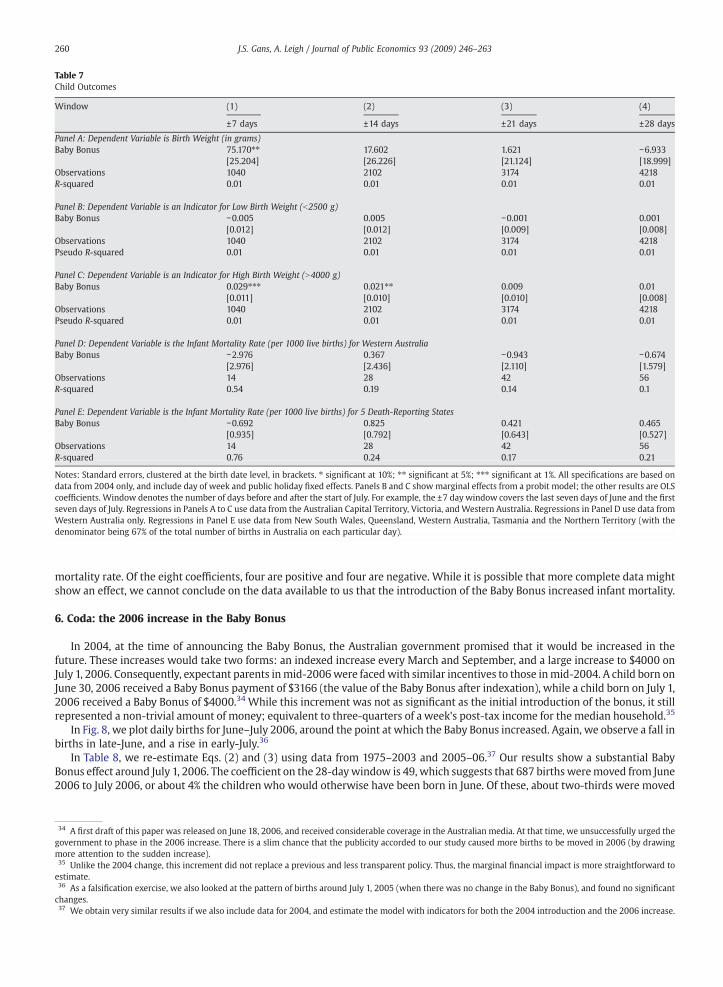
Table 7Child Outcomes
Window (1) (2) (3) (4)
±7 days ±14 days ±21 days ±28 days
Panel A: Dependent Variable is Birth Weight (in grams)Baby Bonus 75.170⁎⁎ 17.602 1.621 −6.933
[25.204] [26.226] [21.124] [18.999]Observations 1040 2102 3174 4218R-squared 0.01 0.01 0.01 0.01
Panel B: Dependent Variable is an Indicator for Low Birth Weight (b2500 g)Baby Bonus −0.005 0.005 −0.001 0.001
[0.012] [0.012] [0.009] [0.008]Observations 1040 2102 3174 4218Pseudo R-squared 0.01 0.01 0.01 0.01
Panel C: Dependent Variable is an Indicator for High Birth Weight (N4000 g)Baby Bonus 0.029⁎⁎⁎ 0.021⁎⁎ 0.009 0.01
[0.011] [0.010] [0.010] [0.008]Observations 1040 2102 3174 4218Pseudo R-squared 0.01 0.01 0.01 0.01
Panel D: Dependent Variable is the Infant Mortality Rate (per 1000 live births) for Western AustraliaBaby Bonus −2.976 0.367 −0.943 −0.674
[2.976] [2.436] [2.110] [1.579]Observations 14 28 42 56R-squared 0.54 0.19 0.14 0.1
Panel E: Dependent Variable is the Infant Mortality Rate (per 1000 live births) for 5 Death-Reporting StatesBaby Bonus −0.692 0.825 0.421 0.465
[0.935] [0.792] [0.643] [0.527]Observations 14 28 42 56R-squared 0.76 0.24 0.17 0.21
Notes: Standard errors, clustered at the birth date level, in brackets. ⁎ significant at 10%; ⁎⁎ significant at 5%; ⁎⁎⁎ significant at 1%. All specifications are based ondata from 2004 only, and include day of week and public holiday fixed effects. Panels B and C showmarginal effects from a probit model; the other results are OLScoefficients. Window denotes the number of days before and after the start of July. For example, the ±7 day window covers the last seven days of June and the firsseven days of July. Regressions in Panels A to C use data from the Australian Capital Territory, Victoria, andWestern Australia. Regressions in Panel D use data fromWestern Australia only. Regressions in Panel E use data from New South Wales, Queensland, Western Australia, Tasmania and the Northern Territory (with thedenominator being 67% of the total number of births in Australia on each particular day).
34 A first draft of this paper was released on June 18, 2006, and received considerable coverage in the Australian media. At that time, we unsuccessfully urged thegovernment to phase in the 2006 increase. There is a slim chance that the publicity accorded to our study caused more births to be moved in 2006 (by drawingmore attention to the sudden increase).35 Unlike the 2004 change, this increment did not replace a previous and less transparent policy. Thus, the marginal financial impact is more straightforward toestimate.36 As a falsification exercise, we also looked at the pattern of births around July 1, 2005 (when there was no change in the Baby Bonus), and found no significanchanges.37 We obtain very similar results if we also include data for 2004, and estimate the model with indicators for both the 2004 introduction and the 2006 increase
260 J.S. Gans, A. Leigh / Journal of Public Economics 93 (2009) 246–263
t
mortality rate. Of the eight coefficients, four are positive and four are negative. While it is possible that more complete data mightshow an effect, we cannot conclude on the data available to us that the introduction of the Baby Bonus increased infant mortality.
6. Coda: the 2006 increase in the Baby Bonus
In 2004, at the time of announcing the Baby Bonus, the Australian government promised that it would be increased in thefuture. These increases would take two forms: an indexed increase every March and September, and a large increase to $4000 onJuly 1, 2006. Consequently, expectant parents inmid-2006were facedwith similar incentives to those inmid-2004. A child born onJune 30, 2006 received a Baby Bonus payment of $3166 (the value of the Baby Bonus after indexation), while a child born on July 1,2006 received a Baby Bonus of $4000.34 While this increment was not as significant as the initial introduction of the bonus, it stillrepresented a non-trivial amount of money; equivalent to three-quarters of a week's post-tax income for the median household.35
In Fig. 8, we plot daily births for June–July 2006, around the point at which the Baby Bonus increased. Again, we observe a fall inbirths in late-June, and a rise in early-July.36
In Table 8, we re-estimate Eqs. (2) and (3) using data from 1975–2003 and 2005–06.37 Our results show a substantial BabyBonus effect around July 1, 2006. The coefficient on the 28-daywindow is 49, which suggests that 687 births weremoved from June2006 to July 2006, or about 4% the children who would otherwise have been born in June. Of these, about two-thirds were moved
t
.
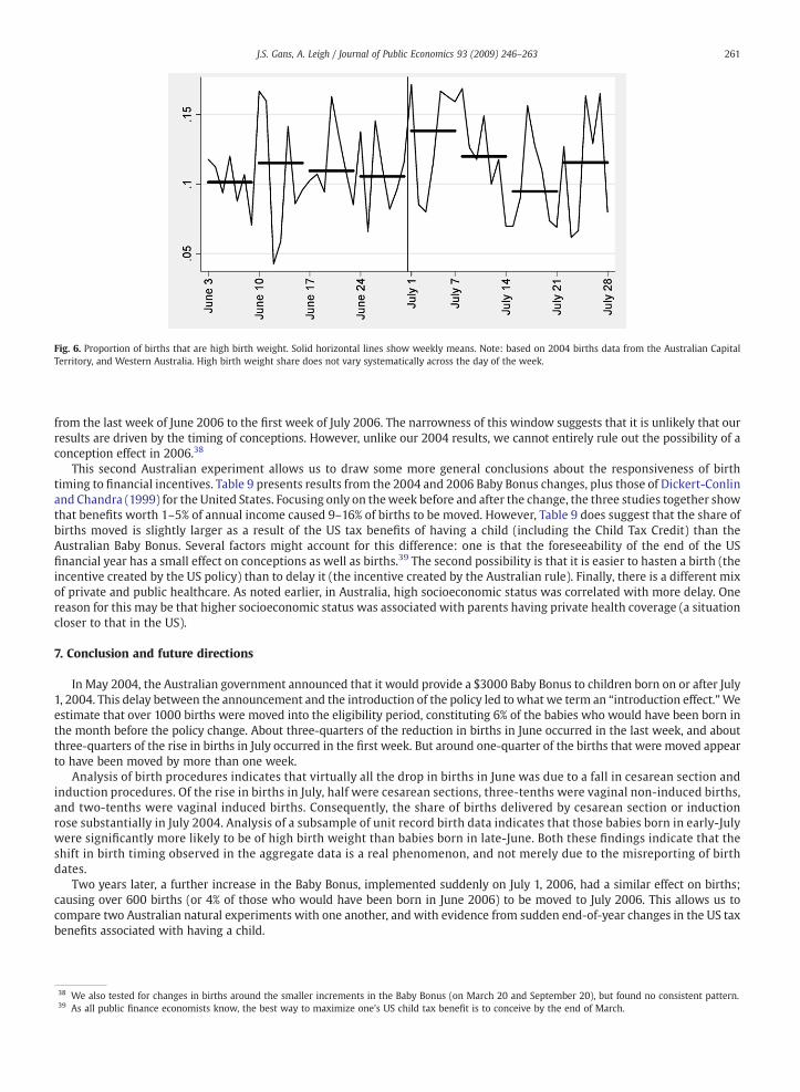
Fig. 6. Proportion of births that are high birth weight. Solid horizontal lines show weekly means. Note: based on 2004 births data from the Australian CapitaTerritory, and Western Australia. High birth weight share does not vary systematically across the day of the week.
38 We also tested for changes in births around the smaller increments in the Baby Bonus (on March 20 and September 20), but found no consistent pattern39 As all public finance economists know, the best way to maximize one's US child tax benefit is to conceive by the end of March.
261J.S. Gans, A. Leigh / Journal of Public Economics 93 (2009) 246–263
l
from the last week of June 2006 to the first week of July 2006. The narrowness of this window suggests that it is unlikely that ourresults are driven by the timing of conceptions. However, unlike our 2004 results, we cannot entirely rule out the possibility of aconception effect in 2006.38
This second Australian experiment allows us to draw some more general conclusions about the responsiveness of birthtiming to financial incentives. Table 9 presents results from the 2004 and 2006 Baby Bonus changes, plus those of Dickert-Conlinand Chandra (1999) for the United States. Focusing only on theweek before and after the change, the three studies together showthat benefits worth 1–5% of annual income caused 9–16% of births to be moved. However, Table 9 does suggest that the share ofbirths moved is slightly larger as a result of the US tax benefits of having a child (including the Child Tax Credit) than theAustralian Baby Bonus. Several factors might account for this difference: one is that the foreseeability of the end of the USfinancial year has a small effect on conceptions as well as births.39 The second possibility is that it is easier to hasten a birth (theincentive created by the US policy) than to delay it (the incentive created by the Australian rule). Finally, there is a different mixof private and public healthcare. As noted earlier, in Australia, high socioeconomic status was correlated with more delay. Onereason for this may be that higher socioeconomic status was associated with parents having private health coverage (a situationcloser to that in the US).
7. Conclusion and future directions
In May 2004, the Australian government announced that it would provide a $3000 Baby Bonus to children born on or after July1, 2004. This delay between the announcement and the introduction of the policy led to what we term an “introduction effect.”Weestimate that over 1000 births were moved into the eligibility period, constituting 6% of the babies who would have been born inthe month before the policy change. About three-quarters of the reduction in births in June occurred in the last week, and aboutthree-quarters of the rise in births in July occurred in the first week. But around one-quarter of the births that were moved appearto have been moved by more than one week.
Analysis of birth procedures indicates that virtually all the drop in births in June was due to a fall in cesarean section andinduction procedures. Of the rise in births in July, half were cesarean sections, three-tenths were vaginal non-induced births,and two-tenths were vaginal induced births. Consequently, the share of births delivered by cesarean section or inductionrose substantially in July 2004. Analysis of a subsample of unit record birth data indicates that those babies born in early-Julywere significantly more likely to be of high birth weight than babies born in late-June. Both these findings indicate that theshift in birth timing observed in the aggregate data is a real phenomenon, and not merely due to the misreporting of birthdates.
Two years later, a further increase in the Baby Bonus, implemented suddenly on July 1, 2006, had a similar effect on births;causing over 600 births (or 4% of those who would have been born in June 2006) to be moved to July 2006. This allows us tocompare two Australian natural experiments with one another, and with evidence from sudden end-of-year changes in the US taxbenefits associated with having a child.
.
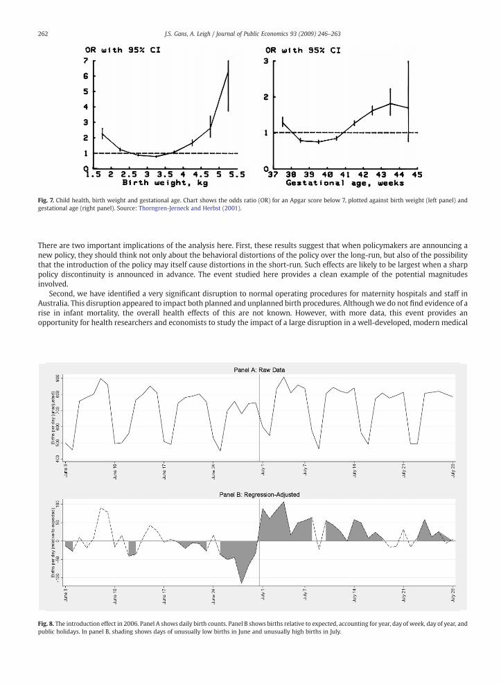
Fig. 8. The introduction effect in 2006. Panel A shows daily birth counts. Panel B shows births relative to expected, accounting for year, day of week, day of year, andpublic holidays. In panel B, shading shows days of unusually low births in June and unusually high births in July.
Fig. 7. Child health, birth weight and gestational age. Chart shows the odds ratio (OR) for an Apgar score below 7, plotted against birth weight (left panel) andgestational age (right panel). Source: Thorngren-Jerneck and Herbst (2001).
262 J.S. Gans, A. Leigh / Journal of Public Economics 93 (2009) 246–263
There are two important implications of the analysis here. First, these results suggest that when policymakers are announcing anew policy, they should think not only about the behavioral distortions of the policy over the long-run, but also of the possibilitythat the introduction of the policy may itself cause distortions in the short-run. Such effects are likely to be largest when a sharppolicy discontinuity is announced in advance. The event studied here provides a clean example of the potential magnitudesinvolved.
Second, we have identified a very significant disruption to normal operating procedures for maternity hospitals and staff inAustralia. This disruption appeared to impact both planned and unplanned birth procedures. Althoughwe do not find evidence of arise in infant mortality, the overall health effects of this are not known. However, with more data, this event provides anopportunity for health researchers and economists to study the impact of a large disruption in a well-developed, modern medical
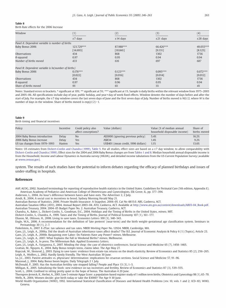
Table 9Birth timing and financial incentives
Policy Incentive Could policy alsoaffect conceptions?
Value (dollars) Value (% of median annualhousehold disposable income)
Share ofbirths moved
2004 Baby Bonus introduction Delay No A$3000 (ignoring previous policy) 5.4% 16.2%2006 Baby Bonus increase Delay Yes A$834 1.4% 9.2%US tax changes from 1979–1993 Hasten Yes US$401 (mean credit, 1996 dollars) 1.1% 13.6%
Notes: US estimates from Dickert-Conlin and Chandra (1999), Table 5. For all studies, effect sizes are based on a ±7 day window, to allow comparability withDickert-Conlin and Chandra (1999). Effect sizes for the 2004 and 2006 Baby Bonus changes are from Tables 1 and 8. Median household annual disposable income ifrom the Household, Income and Labour Dynamics in Australia survey (HILDA), and detailed income tabulations from the US Current Population Survey (availableat www.census.gov).
Table 8Birth Rate effects for the 2006 Increase
Window (1) (2) (3) (4)
±7 days ±14 days ±21 days ±28 days
Panel A: Dependent variable is number of birthsBaby Bonus 2006 123.729⁎⁎⁎ 87.988⁎⁎⁎ 66.426⁎⁎⁎ 49.055⁎⁎⁎
[14.693] [10.841] [9.131] [8.125]Observations 434 868 1302 1736R-squared 0.97 0.95 0.94 0.94Number of births moved 433 616 697 687
Panel B: Dependent variable is ln(number of births)Baby Bonus 2006 0.176⁎⁎⁎ 0.123⁎⁎⁎ 0.095⁎⁎⁎ 0.072⁎⁎⁎
[0.022] [0.016] [0.014] [0.012]Observations 434 868 1302 1736R-squared 0.97 0.96 0.95 0.94Share of births moved 9% 6% 5% 4%
Notes: Standard errors in brackets. ⁎ significant at 10%; ⁎⁎ significant at 5%; ⁎⁎⁎ significant at 1%. Sample is daily births within the relevant window from 1975–2003and 2005–06. All specifications include day of year, public holiday, and year×day of week fixed effects. Window denotes the number of days before and after thestart of July. For example, the ±7 day window covers the last seven days of June and the first seven days of July. Number of births moved is Wβ /2, where W is thenumber of days in the window. Share of births moved is exp(β /2)−1.
263J.S. Gans, A. Leigh / Journal of Public Economics 93 (2009) 246–263
s
system. The results of such studies have the potential to inform debates regarding the efficacy of planned birthdays and issues ofunder-staffing in hospitals.
References
AAP, ACOG, 2002. Standard terminology for reporting of reproductive health statistics in the United States. Guidelines for Perinatal Care (5th edition, Appendix E).American Academy of Pediatrics and American College of Obstetricians and Gynecologists, Elk Grove, IL, pp. 377–394.
Anderson, L., 2004. An hour's difference between haves and have-nots. The Advertiser 2, 2 July.Arndt, B., 2004. A social cost in incentives to breed. Sydney Morning Herald May 21.Australian Bureau of Statistics, 2006. Private Health Insurance: A Snapshot, 2004–05. Cat No 4815.0. ABS, Canberra, ACT.Australian Taxation Office (ATO), 2004. Annual Report 2003–04. ATO, Canberra, ACT. Available at http://www.ato.gov.au/content/downloads/AR03-04_Book.pdf.Australian Treasury, 2004. 2004–05 Budget Paper No. 2. Australian Treasury, Canberra, ACT.Chandra, A., Baker, L., Dickert-Conlin, S., Goodman, D.C., 2004. Holidays and the Timing of Births in the United States, mimeo, MIT.Dickert-Conlin, S., Chandra, A., 1999. Taxes and the Timing of Births. Journal of Political Economy 107 (1), 161–177.Eliason, M., Ohlsson, H., 2008. Living to save taxes. Economics Letters 100 (3), 340–343.Engle, W.A., 2006. A recommendation for the definition of ‘late preterm’ (near-term) and the birth weight–gestational age classification system. Seminars in
Perinatology 30 (1), 2–7.Finkelstein, A., 2007. E-ZTax: tax salience and tax rates. NBER Working Paper No. 12924. NBER, Cambridge, MA.Gans, J.S., Leigh, A., 2006a. Did the death of Australian inheritance taxes affect deaths? The B.E. Journal of Economic Analysis & Policy 6 (1) (Topics), Article 23.Gans, J.S., Leigh, A., 2006b. Bargaining over Labor: Do Patients Have any Power? mimeo, Melbourne.Gans, J.S., Leigh, A., 2007. What Explains the Fall in Weekend Births? mimeo, Melbourne.Gans, J.S., Leigh, A., In press. The Millennium Bub. Applied Economics Letters.Gans, J.S., Leigh, A., Varganova, E., 2007. Minding the shop: the case of obstetrics conferences. Social Science and Medicine 65 (7), 1458–1465.Grattan, M., Nguyen, K., 2004. Baby Bonus tempts teens, claims labor. The Age May 27.Kopczuk, W., Slemrod, J., 2003. Dying to save taxes: evidence from estate-tax returns on the death elasticity. Review of Economics and Statistics 85 (2), 256–265.Leigh, A., Wolfers, J., 2002. Hardly family friendly. The West Australian 30 June.Lo, J.C., 2003. Patient attitudes vs. physicians’ determination: implications for cesarean sections. Social Science and Medicine 57, 91–96.Massoud, J., 2004. Baby Bonus boom begins. Daily Telegraph 2 1 July.McDonald, P., 2005. Has the Australian fertility rate stopped falling? People and Place 13 (3), 1–5.Milligan, K., 2005. Subsidizing the Stork: new evidence on tax incentives and fertility. Review of Economics and Statistics 87 (3), 539–555.Scott, L., 2004. Confined to sitting pretty quiet in the hope of bonus. The Australian 4 29 June.Thorngren-Jerneck, K., Herbst, A., 2001. Low 5-minute Apgar Score: a population-based register study of 1million term births. Obstetrics and Gynecology 98 (1), 65–70.Wells, R., 2004. Women decide: give birth today or take the $3000? The Age 9 30 June.World Health Organization (WHO), 1992. International Statistical Classification of Diseases and Related Health Problems (rev. 10, vols. 1 and 2; ICD-10). WHO,
Geneva.


![BIRTHS, MARRIAGES AND DEATHS [a81y1963]BIRTHS, … · any births, marriages or deaths registration office in existence prior to the commencement of this Act. (2) The Secretary may](https://img.pdfslide.us/doc/110x75/60dc4d3f4aae351d7570c520/births-marriages-and-deaths-a81y1963births-any-births-marriages-or-deaths-registration.jpg)