Embed Size (px)
Citation preview
M
Oa
b
a
ARRAA
KRDDDTAs
1
ifip[tca
uDat
CpdbaDs
(
0d
Journal of Process Control 22 (2012) 41– 50
Contents lists available at SciVerse ScienceDirect
Journal of Process Control
jo u rn al hom epa ge: ww w.elsev ier .com/ locate / jprocont
odel-based temperature control of a diesel oxidation catalyst
livier Lepreuxa,∗, Yann Creff a, Nicolas Petitb
IFP Energies nouvelles, Technology, Computer Science and Applied Mathematics Division, BP 3, 69360 Solaize, FranceMINES ParisTech, Centre Automatique et Système, Mathématiques et Systémes, 60 bd. Saint-Michel, 75272 Paris Cedex 06, France
r t i c l e i n f o
rticle history:eceived 22 April 2011eceived in revised form 7 September 2011ccepted 19 October 2011vailable online 23 November 2011
eywords:educed model
a b s t r a c t
The problem studied in this article is the control of a DOC (diesel oxidation catalyst) as used in aftertreat-ment systems of diesel vehicles. This system is inherently a distributed parameter system due to itselongated geometry where a gas stream is in contact with a spatially distributed catalyst. A first con-tribution is a model for the DOC system. It is obtained by successive simplifications justified eitherexperimentally (from observations, estimates of orders of magnitude) or by an analysis of governingequations (through asymptotic developments and changes of variables). This model can reproduce thecomplex temperature response of DOC output to changes in input variables. In particular, the effects of
istributed parameter systemselay systemsiesel oxidation catalystemperature controlutomotive exhaust aftertreatment
gas velocity variations, inlet temperature and inlet hydrocarbons are well represented. A second contri-bution is a combination of algorithms (feedback, feedforward, and synchronization) designed to controlthe thermal phenomena in the DOC. Both contributions have been tested and validated experimentally.In conclusion, the outcomes are evaluated: using the approach presented in this article, it is possible tocontrol, in conditions representative of vehicle driving conditions, the outlet temperature of the DOC
◦
ystems within ±15 C.. Introduction
On most new diesel vehicles, increasing requirements regard-ng particulate matter emissions [1] are met using diesel particulatelters (DPF). This filter, located in the vehicle exhaust line, storesarticulate matter until it is burnt in an active regeneration process2]. During this phase, DPFs behave like potentially unstable reac-ors [3]. Consequently, their inlet temperature must be carefullyontrolled to prevent filter runaway. As is now exposed, this can beccomplished by the diesel oxidation catalyst (DOC).
In most current aftertreatment architectures [4], a DOC is placedpstream of the DPF in the vehicle exhaust line. To increase thePF inlet temperature, reductants – mostly hydrocarbons (HC) –re oxidized in the DOC, which, in turn, increases the DOC outletemperature, and therefore the DPF inlet temperature.
A DOC is a chemical system difficult to model and to control.lassical DOC models are usually composed of a dozen of coupledartial differential equations (PDEs) [5], which make difficult theevelopment of model-based control laws. Experimentally, it haseen observed that a step change on the inlet temperature prop-
gates to the output of the system with large response times [6].epending on the engine outlet gas velocity, these response timesignificantly vary: they roughly decrease by a factor of 10 from
∗ Corresponding author.E-mail addresses: [email protected] (O. Lepreux), [email protected]
Y. Creff), [email protected] (N. Petit).
959-1524/$ – see front matter © 2011 Elsevier Ltd. All rights reserved.oi:10.1016/j.jprocont.2011.10.012
© 2011 Elsevier Ltd. All rights reserved.
idle speed to full load. Strategies that are commonly used to dealwith this problem rely on controller gain look-up tables, which, inpractice, are difficult and time-consuming to calibrate.
The purpose of this paper is to propose a simple model dedicatedto the DOC outlet temperature control during DPF regeneration alongwith a control law. To achieve this, a simplification of the above-mentioned classical models is performed.
The paper is organized as follows. In Section 2.1 the control prob-lem is exposed. In Section 2.2 the experimental setup is presented.The Section 3 presents a model describing the thermal responsesproperly. This model is physics-based. In Section 4, a control strat-egy based on the proposed model, which is further simplified, isdeveloped. It is divided into three parts: (i) a feedforward con-trol for the inlet temperature (disturbance); (ii) a simple integralaction; (iii) a feedforward control to attenuate the effects of thegas velocity variations (disturbance). The proposed strategy sched-ules the adaptation of parameters of the control law according tothe varying gas velocity. To stress the relevance of the contribu-tion, experimental control results are presented and discussed inSection 5.
2. Control problem
2.1. Input–output description
The paper focuses on the dynamics of the simple system pic-tured in Fig. 1, for which the steady-state effects are easily captured.
42 O. Lepreux et al. / Journal of Proce
Fa
Tdvrrs
iac
2
tTituitcopeDoa
(ep
m
3
nT
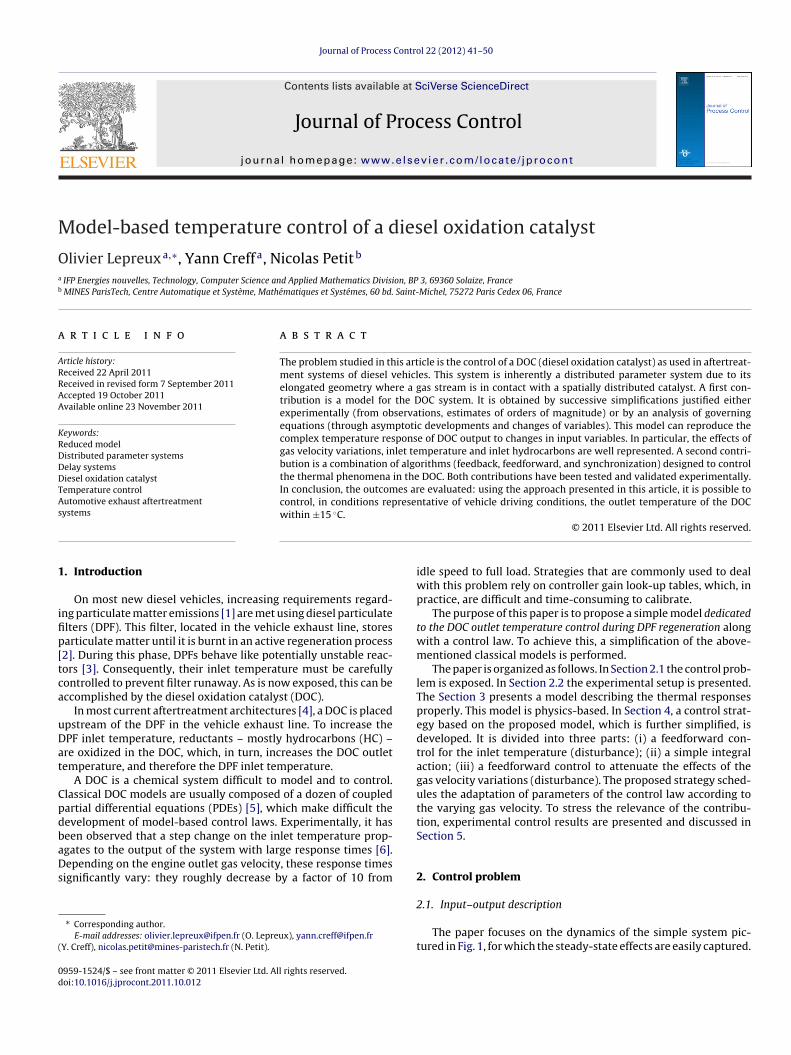
ig. 1. DOC input–output description. The control is u, the output is Tout, while Tin
nd v are disturbances.
he inputs are the control variable u (control HC flow rate), theisturbance variable Tin (inlet temperature), and the disturbanceariable v (gas velocity). This latter disturbance defines the gas flowate (F), which is of practical interest. A straightforward relationelates the gas flow rate and the gas velocity (see below (20)). Theystem output is the outlet gas temperature Tout.
Certainly, the real picture of the DOC is more complicated, as itnvolves several other disturbances, among which is, in particular,n undesired reductants flow. Detailed discussions on this pointan be found in [7].
.2. Experimental setup
The experimental setup is depicted in Fig. 2 and presented inhe following. The DOC is located in a Diesel engine exhaust line.he engine operating point imposes the gas velocity and the DOCnlet temperature. Two distinct configurations are used to controlhe reductants flow: either by an additional injector located rightpstream of the turbine or by in-cylinder late post-injection. It
s worth mentioning that the HCs generated by these two injec-ion methods are different and can actually affect the overall DOConversion efficiency [8]. This effect can be significant at someperating points. Values obtained in this paper depend on eacharticular tested system. Temperature is measured at three differ-nt locations and gas is analyzed upstream and downstream of theOC by a 5-gas sensor. Presented experimental results have beenbtained using two distinct engines and DOC setups. A 3-in. longnd a 4-in. long platinum-based DOC have been tested.
Considering those configurations, generating a disturbanceengine emissions, Tin, gas velocity) independently from the oth-rs is not possible. This explains why they are not decoupled in theresented results.
The system is tested in an engine test cell, not in a vehicle. Thisay impact some results about heat losses.
. Reduced model
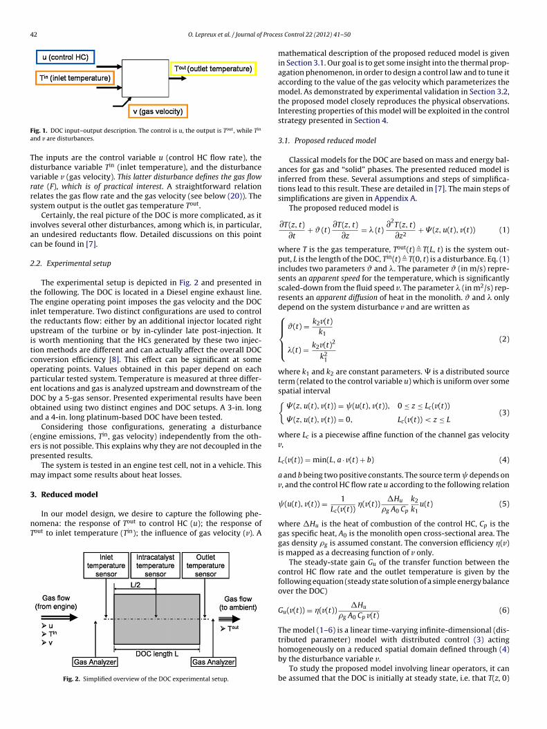
In our model design, we desire to capture the following phe-omena: the response of Tout to control HC (u); the response ofout to inlet temperature (Tin); the influence of gas velocity (v). A
Fig. 2. Simplified overview of the DOC experimental setup.
ss Control 22 (2012) 41– 50
mathematical description of the proposed reduced model is givenin Section 3.1. Our goal is to get some insight into the thermal prop-agation phenomenon, in order to design a control law and to tune itaccording to the value of the gas velocity which parameterizes themodel. As demonstrated by experimental validation in Section 3.2,the proposed model closely reproduces the physical observations.Interesting properties of this model will be exploited in the controlstrategy presented in Section 4.
3.1. Proposed reduced model
Classical models for the DOC are based on mass and energy bal-ances for gas and “solid” phases. The presented reduced model isinferred from these. Several assumptions and steps of simplifica-tions lead to this result. These are detailed in [7]. The main steps ofsimplifications are given in Appendix A.
The proposed reduced model is
∂T(z, t)∂t
+ ϑ (t)∂T(z, t)∂z
= � (t)∂2T(z, t)∂z2
+ � (z, u(t), v(t)) (1)
where T is the gas temperature, Tout(t) � T(L, t) is the system out-put, L is the length of the DOC, Tin(t) � T(0, t) is a disturbance. Eq. (1)includes two parameters ϑ and �. The parameter ϑ (in m/s) repre-sents an apparent speed for the temperature, which is significantlyscaled-down from the fluid speed v. The parameter � (in m2/s) rep-resents an apparent diffusion of heat in the monolith. ϑ and � onlydepend on the system disturbance v and are written as⎧⎪⎪⎨⎪⎪⎩ϑ(t) = k2v(t)
k1
�(t) = k2v(t)2
k21
(2)
where k1 and k2 are constant parameters. � is a distributed sourceterm (related to the control variable u) which is uniform over somespatial interval{� (z, u(t), v(t)) = (u(t), v(t)), 0 ≤ z ≤ Lc(v(t))
� (z, u(t), v(t)) = 0, Lc(v(t)) < z ≤ L(3)
where Lc is a piecewise affine function of the channel gas velocityv,
Lc(v(t)) = min(L, a · v(t) + b) (4)
a and b being two positive constants. The source term depends onv, and the control HC flow rate u according to the following relation
(u(t), v(t)) = 1Lc(v(t))
�(v(t))�Hug A0 Cp
k2
k1u(t) (5)
where �Hu is the heat of combustion of the control HC, Cp is thegas specific heat, A0 is the monolith open cross-sectional area. Thegas density g is assumed constant. The conversion efficiency �(v)is mapped as a decreasing function of v only.
The steady-state gain Gu of the transfer function between thecontrol HC flow rate and the outlet temperature is given by thefollowing equation (steady state solution of a simple energy balanceover the DOC)
Gu(v(t)) = �(v(t))�Hu
g A0 Cp v(t)(6)
The model (1–6) is a linear time-varying infinite-dimensional (dis-tributed parameter) model with distributed control (3) acting
homogeneously on a reduced spatial domain defined through (4)by the disturbance variable v.To study the proposed model involving linear operators, it canbe assumed that the DOC is initially at steady state, i.e. that T(z, 0)
O. Lepreux et al. / Journal of Process Control 22 (2012) 41– 50 43
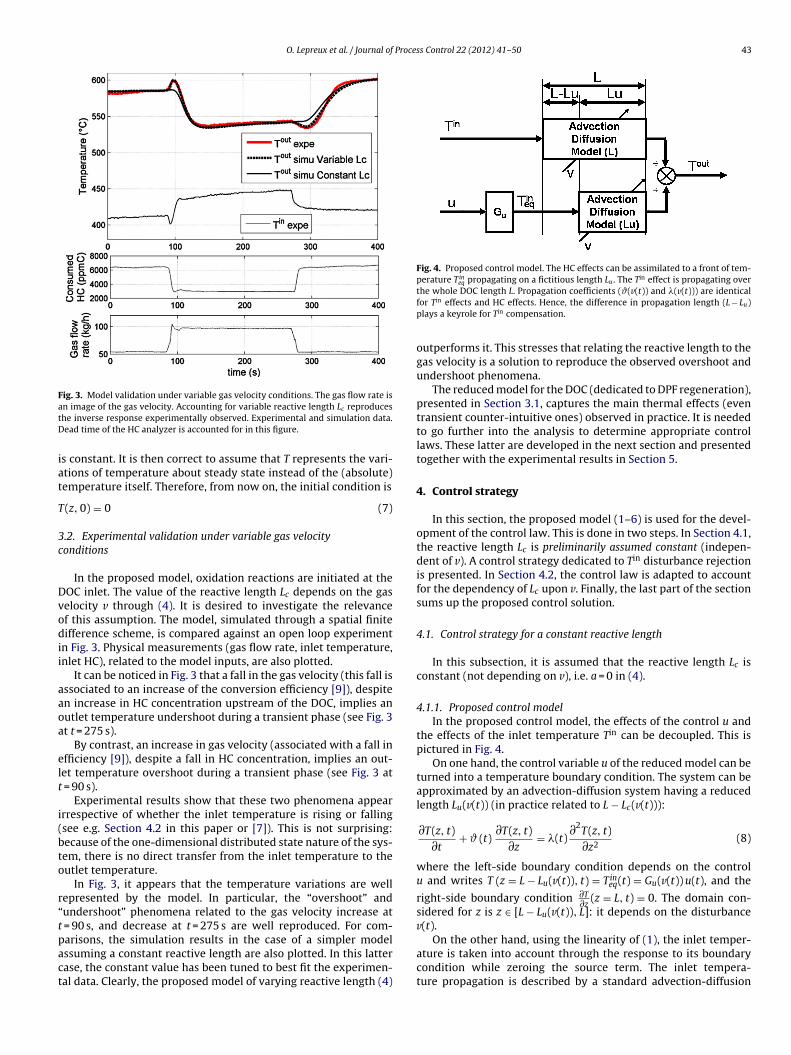
Fig. 3. Model validation under variable gas velocity conditions. The gas flow rate isatD
iat
T
3c
Dvodii
aaoa
elt
i(bto
r“tpact
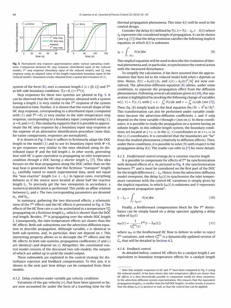
Fig. 4. Proposed control model. The HC effects can be assimilated to a front of tem-perature Tineq propagating on a fictitious length Lu . The Tin effect is propagating over
n image of the gas velocity. Accounting for variable reactive length Lc reproduceshe inverse response experimentally observed. Experimental and simulation data.ead time of the HC analyzer is accounted for in this figure.
s constant. It is then correct to assume that T represents the vari-tions of temperature about steady state instead of the (absolute)emperature itself. Therefore, from now on, the initial condition is
(z, 0) = 0 (7)
.2. Experimental validation under variable gas velocityonditions
In the proposed model, oxidation reactions are initiated at theOC inlet. The value of the reactive length Lc depends on the gaselocity v through (4). It is desired to investigate the relevancef this assumption. The model, simulated through a spatial finiteifference scheme, is compared against an open loop experiment
n Fig. 3. Physical measurements (gas flow rate, inlet temperature,nlet HC), related to the model inputs, are also plotted.
It can be noticed in Fig. 3 that a fall in the gas velocity (this fall isssociated to an increase of the conversion efficiency [9]), despiten increase in HC concentration upstream of the DOC, implies anutlet temperature undershoot during a transient phase (see Fig. 3t t = 275 s).
By contrast, an increase in gas velocity (associated with a fall infficiency [9]), despite a fall in HC concentration, implies an out-et temperature overshoot during a transient phase (see Fig. 3 at
= 90 s).Experimental results show that these two phenomena appear
rrespective of whether the inlet temperature is rising or fallingsee e.g. Section 4.2 in this paper or [7]). This is not surprising:ecause of the one-dimensional distributed state nature of the sys-em, there is no direct transfer from the inlet temperature to theutlet temperature.
In Fig. 3, it appears that the temperature variations are wellepresented by the model. In particular, the “overshoot” andundershoot” phenomena related to the gas velocity increase at
= 90 s, and decrease at t = 275 s are well reproduced. For com-
arisons, the simulation results in the case of a simpler modelssuming a constant reactive length are also plotted. In this latterase, the constant value has been tuned to best fit the experimen-al data. Clearly, the proposed model of varying reactive length (4)the whole DOC length L. Propagation coefficients (ϑ(v(t)) and �(v(t))) are identicalfor Tin effects and HC effects. Hence, the difference in propagation length (L − Lu)plays a keyrole for Tin compensation.
outperforms it. This stresses that relating the reactive length to thegas velocity is a solution to reproduce the observed overshoot andundershoot phenomena.
The reduced model for the DOC (dedicated to DPF regeneration),presented in Section 3.1, captures the main thermal effects (eventransient counter-intuitive ones) observed in practice. It is neededto go further into the analysis to determine appropriate controllaws. These latter are developed in the next section and presentedtogether with the experimental results in Section 5.
4. Control strategy
In this section, the proposed model (1–6) is used for the devel-opment of the control law. This is done in two steps. In Section 4.1,the reactive length Lc is preliminarily assumed constant (indepen-dent of v). A control strategy dedicated to Tin disturbance rejectionis presented. In Section 4.2, the control law is adapted to accountfor the dependency of Lc upon v. Finally, the last part of the sectionsums up the proposed control solution.
4.1. Control strategy for a constant reactive length
In this subsection, it is assumed that the reactive length Lc isconstant (not depending on v), i.e. a = 0 in (4).
4.1.1. Proposed control modelIn the proposed control model, the effects of the control u and
the effects of the inlet temperature Tin can be decoupled. This ispictured in Fig. 4.
On one hand, the control variable u of the reduced model can beturned into a temperature boundary condition. The system can beapproximated by an advection-diffusion system having a reducedlength Lu(v(t)) (in practice related to L − Lc(v(t))):
∂T(z, t)∂t
+ ϑ (t)∂T(z, t)∂z
= �(t)∂2T(z, t)∂z2
(8)
where the left-side boundary condition depends on the controlu and writes T (z = L − Lu(v(t)), t) = Tineq(t) = Gu(v(t)) u(t), and the
right-side boundary condition ∂T∂z
(z = L, t) = 0. The domain con-sidered for z is z ∈ [L − Lu(v(t)), L]: it depends on the disturbancev(t).
On the other hand, using the linearity of (1), the inlet temper-ature is taken into account through the response to its boundarycondition while zeroing the source term. The inlet tempera-ture propagation is described by a standard advection-diffusion
44 O. Lepreux et al. / Journal of Proce
0 20 40 60 800
0.5
1
time (s)
Nor
mal
ized
tem
pera
ture
0 50 100 1500
0.5
1
time (s)
Nor
mal
ized
tem
pera
ture
Tin step resp.HC step resp.
AdaptedTin step resp.
v=3.8m/s v=1.9m/s
Fig. 5. Normalized step response approximation under various operating condi-tions. Comparison between HC step response (distributed input of the reducedmrr
sa
chtHwr itf
ltthcfwLtblnba
veprLHtbiHato
tsm
4
a
4.1.4. Feedback controlAs detailed before, control HC effects for a catalyst length L are
equivalent to boundary temperature effects for a catalyst length
1 Note that analytic responses to HC and Tin have been compared in Fig. 5 (using
odel), Tin step response (boundary input of the reduced model), and Tineq stepesponse using an adapted value of the length (equivalent boundary input of theeduced model). Simulation results obtained from a spatial discretization of (1).
ystem of the form (8), over a constant length L (z ∈ [0, L]) and Tin
s left-side boundary condition: T(z = 0, t) = Tin(t).Step responses for these two systems are plotted in Fig. 5. It
an be observed that the HC step response, obtained with a systemaving a length L is very similar to the Tin response of the systemranslated in time. Further, it is shown that the overall shape of theC step response, corresponding to a distributed input (computedith (1) and Tin = 0), is very similar to the inlet temperature step
esponse, corresponding to a boundary input (computed using (1), = 0, and z = L). This similarity supports that it is possible to approx-
mate the HC step response by a boundary input step response athe expense of an alternative identification procedure (note that,or easier comparisons, responses are normalized).
It is shown in Fig. 5 that it suffices to fictitiously adapt the DOCength in the model (1) and to use its boundary input with � = 0,o get responses very similar to the ones obtained using its dis-ributed input � and the full length L. In other words, generatingeat with HC is quite equivalent to propagating an inlet temperatureondition through a DOC having a shorter length Lu [7]. This ideaocuses on the heat propagation along the DOC rather than on theay heat is generated. Note that this fictitious “transport” length
u, carefully tuned to match experimental data, need not equalhe “non-reactive” length (i.e. L − Lc). In typical cases, everythingehaves as if the source were located at about half the reactive
ength Lc. To precisely get the two viewpoints in accordance, aumerical identification is performed. This yields an affine relationetween Lu and v. The two corresponding parameters are denotedLu and bLu .
In summary, gathering the two discussed effects, a schematiciew of the Tin effects and the HC effects is presented in Fig. 4. Theffects of the HC flow rate u can be assimilated to a temperature Tineqropagating on a fictitious length Lu, which is shorter than the DOCeal length. Besides, Tin is propagating over the whole DOC length. Consequently, the inlet temperature effects are slower than theC effects. Both sub-subsystems use the advection-diffusion equa-
ion to describe propagation. Although variable, v is identical inoth sub-systems, and, in particular, does not depend on z. This
nteresting property allows us to decouple the Tin effects and theC effects. In both sub-systems, propagation coefficients (ϑ and �)re identical (and depend on v). Altogether, the constituted con-rol model consists of the discussed two sub-models, the outputsf which are added up to yield the model output.
These submodels are exploited in the control strategy for dis-urbance rejection and feedback compensation. To this aim, it ishown in the next part how delays can be computed from theseodels.
.1.2. Delay evolution under variable gas velocity conditionsVariations of the gas velocity (v), that have been ignored so far,
re now accounted for under the form of a traveling time for the
ss Control 22 (2012) 41– 50
thermal propagation phenomena. This time ı(t) will be used in thecontrol design.
Consider the delay ı(t) defined by T(z, t) = T(z − zp, t − ı(t)) wherezp represents the considered length of propagation. It can be shown(see e.g. [7]) that the delay evolution satisfies the following implicitequation, in which ı(t) is unknown
zp =∫ t
t−ı(t)ϑ(w)dw (9)
This implicit equation will be used to describe the evolution of ther-mal phenomena and, in particular, to synchronize the control actionwith the measured disturbance.
To simplify the calculation, it has been assumed that the approx-imations that have led to the reduced model hold when v depends ontime. Hence, ϑ(t) = k2v(t)/k1 and �(t) = k2v(t)2/k2
1 are now con-sidered. The advection-diffusion equation (8) allows, under someconditions, to separate the propagation effect from the diffusionphenomenon. Following several calculations given in [10], this sep-aration is highlighted by invoking the following change of variablesw(, �) = T(z, t), with = z −
∫ t0ϑ(s)ds and � =
∫ t0�(s)ds (see [7]).
Then, Eq. (8) simply leads to the heat equation ∂w/∂� = ∂2w/∂2.
This transformation can also be performed under variable condi-tions because the advection-diffusion coefficients � and ϑ onlydepend on the time variable t through v (not on z). In these coordi-nates, it is possible to study the propagation on a system having aninfinite length. In this infinite-length system, the boundary condi-tions are located at =± ∞ in the (, �)-coordinates or at z =± ∞ inthe (z, t)-coordinates. It is considered that the boundaries are “far”from the studied phenomena (relatively to diffusion effects). Then,under these conditions, it is possible to solve (9) with respect to thepropagation delay ı(t). The reader can refer to [7] for more details.
4.1.3. Feedforward control strategy for a constant reactive lengthIt is possible to compensate for effects of Tin by synchronization
with delayed effects of u. As pictured in Fig. 4, the synchronizationbetween Tin and u must be considered on the first part of the DOCfor the length difference L − Lu. Hence, from the advection-diffusionmodel viewpoint, the delay ıFF(t) to synchronize the inlet temper-ature variations with the control HC variations is simply given bythe implicit equation, in which ıFF(t) is unknown and ϑ representsan apparent propagation speed1:
L − Lu =∫ t
t−ıFF (t)
ϑ(w)dw (10)
Finally, a feedforward compensation block for the Tin distur-bance can be simply based on a delay operator applying a delayvalue of ıFF(t)
uFF (t) = 1
Gdynu (t)Tin(t − ıFF (t)) (11)
where uFF is the feedforward HC flow to deliver in order to rejectTin variations, and where Gdynu is a dynamically updated version ofGu that will be detailed in Section 4.2.
the reduced model). It has been shown that inlet temperature effects are slower thanHC effects. It is then theoretically possible to compensate totally for these variations.In the advection-diffusion system representation, this ensures that the equivalentpropagation length Lu is smaller than the full DOC length L. In other words, it ensuresthat the delay ıFF(t) is positive or null, so that the control law can be applied.
Process Control 22 (2012) 41– 50 45
Ls4o
L
Fo
ptaTaif(sns
i5
�
Tif
u
w
v
4
bcol
sdrpaaito
ir
otcvrAr
O. Lepreux et al. / Journal of
u. A variation of HC is interpreted as a boundary condition Tineq(t) ofystem (8) over a propagation length Lu. Applying results of Section.1.2, HC response time calculation can be based on the evaluationf the following implicit equation in which ıFB is the unknown:
u =∫ t
t−ıFB(t)
ϑ(�)d� (12)
or an HC step input, ıFB is approximately the time at which theutlet temperature reaches half its steady-state value.
As will be developed in Section 4.2, in practice, DOC outlet tem-erature cannot be perfectly controlled due to changes (slips) ofhe reactive zone during gas velocity variations. Induced overshootnd undershoot phenomena have been discussed in Section 3.2.ypically, for a 4-in. long DOC, practical achievable performance isbout ±15 ◦C. This observation is a big concern because this results close to the performance requested for real applications. There-ore, the feedback control in this zone cannot be totally turned offas would be done for example by a usually considered deadzonetrategy) but it has to be loosely tuned. Typically, in this zone, it isot possible to use a classic feedback control law because error toetpoint is related to hardly compensable disturbance effects.
To compensate for steady-state errors, a simple integral actions used. To obtain the results presented in this paper (see Section), the integral time is empirically set to
i = 2 · ıFB (13)
his means that, for a given gas velocity, the integral time is approx-mately set equal to the duration of the HC effect. Finally, theeedback action of the controller is given by a simple integral term
FB(t) = 1
Gdynu (t)
∫ t
0
1�i(w)
(Tsp(w) − Tout(w)
)dw (14)
here Tsp is the outlet temperature setpoint.Note that adaptations of this law can be used for large setpoint
ariations [11].
.2. Generalization of the control law for variable gas velocity
In the previous subsection, the dependence of Lc upon v, statedy (4), has been ignored. In this subsection, it is shown how theontrol law previously developed can be adapted to account for thevershoot and undershoot phenomena, i.e. for a variable reactiveength Lc.
The overshoot phenomenon stems from the combination of heattorage and under-actuation effects, on a reactive length that isefined by a disturbance, namely the gas velocity. We refer theeader interested by the origins of the overshoot to [9,7], where a sim-le advection model is used to illustrate this point. The presentednalytic study shows that an increase in the reactive length causesn overshoot. An analytic control trajectory to limit the overshoots proposed in [9]: when the gas velocity increases, the static gain isransiently decreased in order to limit the coming overshoot. Thisvershoot compensation induces an undershoot.
In the following, a specific feedforward control law that closelymitates this approach is presented and open loop experiments areeported.
An easy-to-implement dynamic gain adaptation is used, basedn the time derivative of the gas velocity. A filtered derivative ofhe speed v(t) is computed. The filter is a first order filter with timeonstant �B. The filtered derivative is normalized with the current
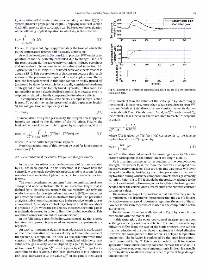
alue of the gas velocity, and multiplied by a gain KB to give a cor-ection term X. The gain Gdynu used is given by Gdynu = Gu/(1 − X).ccording to this relation, a rise (resp. decrease) of v(t) induces aise (resp. decrease) of X: the value Gdynu of the gain is then largerFig. 6. Illustration of overshoot compensation based on gas velocity derivative.Simulation data.
(resp. smaller) than the values of the static gain Gu. Accordingly,the control u is less (resp. more) than what is required to keep Tout
constant. While v(t) stabilizes to a new constant value, its deriva-tive tends to 0. Then, X tends toward 0 and, as Gdynu tends toward Gu,the control u takes the value that is required to reach Tout setpoint.In details,
1
Gdynu (v(t))= 1 − X(t)Gu(v(t))
(15)
where X(t) is given by Y(t)/v(t), Y(t) corresponds to the inverseLaplace transform of Y(s) given by
Y(s) = KBs
1 + �Bsvsat (16)
and vsat is the saturated value of the current gas velocity. This sat-uration corresponds to the saturation of the length Lc in (4).
KB is a tuning parameter corresponding to the compensationstrength. The greater KB is, the more the control u is adapted dur-ing gas velocity transients. If set too high, this parameter will favordelayed side effects. Besides, �B is a tuning parameter correspond-ing to a time during which the compensation acts after a gas velocityvariation. Referring to [7], it should be theoretically adapted to thecurrent variation of Lc. However, in practice, this extra tuning is notneeded since the correction is already quite efficient with constantparameter values.
The main advantage of this method is that it is extremely simpleto implement. It is also interesting to notice that the use of a filteredderivative ensures a good robustness regarding the noise of the airflow sensor measurement which is used in the computation of thegas velocity.
The behavior of the law is illustrated in Fig. 6 by a simulation,carried out with the model (19).
In this simulation, the open loop control strategy acts as soonas the gas velocity variation is detected. The control variable sig-nificantly differs from the case of the static strategy. One can seethat the reduction of the overshoot magnitude is indeed effective.However, the consequence of this action is a delayed temperatureundershoot. The behavior is confirmed by the open loop experi-ment presented in Fig. 7. This is an important result for control
application since undershooting does not increase the risks of DPFrunaway. However, overshoot compensation is limited: it is usuallybetter to allow a small overshoot in order to prevent large delayedundershooting.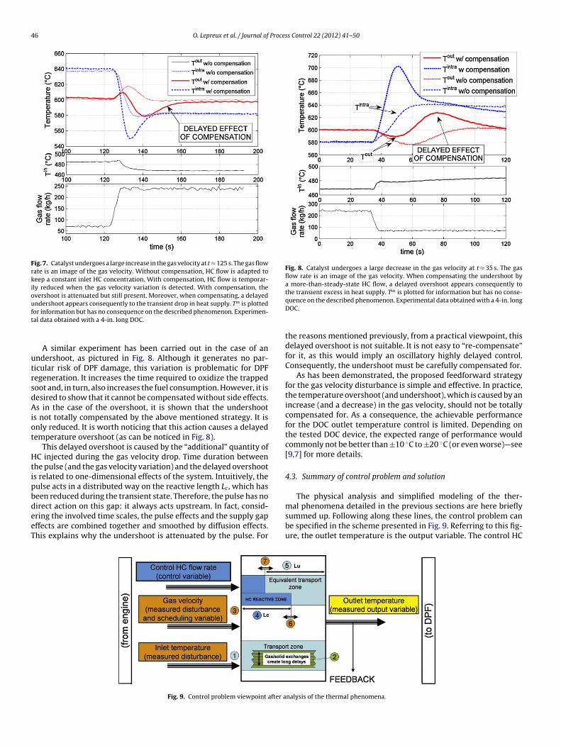
46 O. Lepreux et al. / Journal of Process Control 22 (2012) 41– 50
Fig. 7. Catalyst undergoes a large increase in the gas velocity at t ≈ 125 s. The gas flowrate is an image of the gas velocity. Without compensation, HC flow is adapted tokeep a constant inlet HC concentration. With compensation, HC flow is temporar-ily reduced when the gas velocity variation is detected. With compensation, theovershoot is attenuated but still present. Moreover, when compensating, a delayedundershoot appears consequently to the transient drop in heat supply. Tin is plottedft
utrsdAiot
HtipbdeeT
Fig. 8. Catalyst undergoes a large decrease in the gas velocity at t ≈ 35 s. The gasflow rate is an image of the gas velocity. When compensating the undershoot bya more-than-steady-state HC flow, a delayed overshoot appears consequently tothe transient excess in heat supply. Tin is plotted for information but has no conse-
mal phenomena detailed in the previous sections are here briefly
or information but has no consequence on the described phenomenon. Experimen-al data obtained with a 4-in. long DOC.
A similar experiment has been carried out in the case of anndershoot, as pictured in Fig. 8. Although it generates no par-icular risk of DPF damage, this variation is problematic for DPFegeneration. It increases the time required to oxidize the trappedoot and, in turn, also increases the fuel consumption. However, it isesired to show that it cannot be compensated without side effects.s in the case of the overshoot, it is shown that the undershoot
s not totally compensated by the above mentioned strategy. It isnly reduced. It is worth noticing that this action causes a delayedemperature overshoot (as can be noticed in Fig. 8).
This delayed overshoot is caused by the “additional” quantity ofC injected during the gas velocity drop. Time duration between
he pulse (and the gas velocity variation) and the delayed overshoots related to one-dimensional effects of the system. Intuitively, theulse acts in a distributed way on the reactive length Lc, which haseen reduced during the transient state. Therefore, the pulse has noirect action on this gap: it always acts upstream. In fact, consid-
ring the involved time scales, the pulse effects and the supply gapffects are combined together and smoothed by diffusion effects.his explains why the undershoot is attenuated by the pulse. ForFig. 9. Control problem viewpoint after a
quence on the described phenomenon. Experimental data obtained with a 4-in. longDOC.
the reasons mentioned previously, from a practical viewpoint, thisdelayed overshoot is not suitable. It is not easy to “re-compensate”for it, as this would imply an oscillatory highly delayed control.Consequently, the undershoot must be carefully compensated for.
As has been demonstrated, the proposed feedforward strategyfor the gas velocity disturbance is simple and effective. In practice,the temperature overshoot (and undershoot), which is caused by anincrease (and a decrease) in the gas velocity, should not be totallycompensated for. As a consequence, the achievable performancefor the DOC outlet temperature control is limited. Depending onthe tested DOC device, the expected range of performance wouldcommonly not be better than ±10 ◦C to ±20 ◦C (or even worse)—see[9,7] for more details.
4.3. Summary of control problem and solution
The physical analysis and simplified modeling of the ther-
summed up. Following along these lines, the control problem canbe specified in the scheme presented in Fig. 9. Referring to this fig-ure, the outlet temperature is the output variable. The control HC
nalysis of the thermal phenomena.
Process Control 22 (2012) 41– 50 47
fl(trtroaafTrasacaii
pFs(ba(u
taap
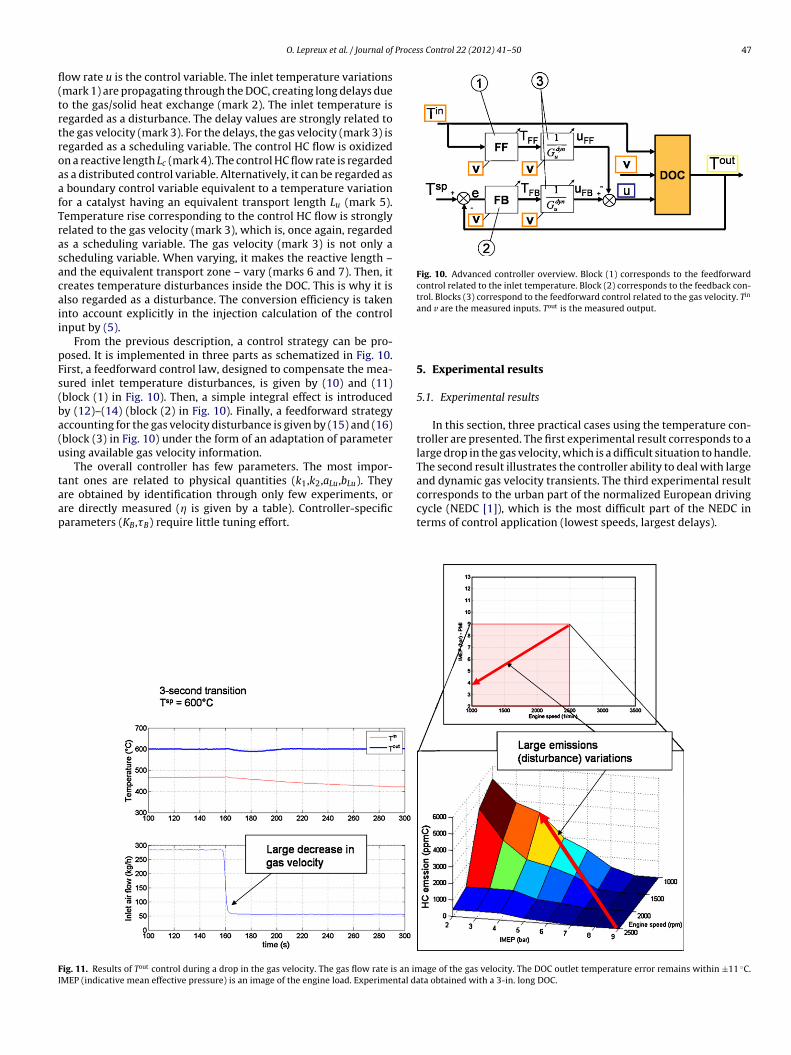
Fig. 10. Advanced controller overview. Block (1) corresponds to the feedforwardcontrol related to the inlet temperature. Block (2) corresponds to the feedback con-trol. Blocks (3) correspond to the feedforward control related to the gas velocity. Tin
and v are the measured inputs. Tout is the measured output.
FI
O. Lepreux et al. / Journal of
ow rate u is the control variable. The inlet temperature variationsmark 1) are propagating through the DOC, creating long delays dueo the gas/solid heat exchange (mark 2). The inlet temperature isegarded as a disturbance. The delay values are strongly related tohe gas velocity (mark 3). For the delays, the gas velocity (mark 3) isegarded as a scheduling variable. The control HC flow is oxidizedn a reactive length Lc (mark 4). The control HC flow rate is regardeds a distributed control variable. Alternatively, it can be regarded as
boundary control variable equivalent to a temperature variationor a catalyst having an equivalent transport length Lu (mark 5).emperature rise corresponding to the control HC flow is stronglyelated to the gas velocity (mark 3), which is, once again, regardeds a scheduling variable. The gas velocity (mark 3) is not only acheduling variable. When varying, it makes the reactive length –nd the equivalent transport zone – vary (marks 6 and 7). Then, itreates temperature disturbances inside the DOC. This is why it islso regarded as a disturbance. The conversion efficiency is takennto account explicitly in the injection calculation of the controlnput by (5).
From the previous description, a control strategy can be pro-osed. It is implemented in three parts as schematized in Fig. 10.irst, a feedforward control law, designed to compensate the mea-ured inlet temperature disturbances, is given by (10) and (11)block (1) in Fig. 10). Then, a simple integral effect is introducedy (12)–(14) (block (2) in Fig. 10). Finally, a feedforward strategyccounting for the gas velocity disturbance is given by (15) and (16)block (3) in Fig. 10) under the form of an adaptation of parametersing available gas velocity information.
The overall controller has few parameters. The most impor-
ant ones are related to physical quantities (k1,k2,aLu,bLu). Theyre obtained by identification through only few experiments, orre directly measured (� is given by a table). Controller-specificarameters (KB,�B) require little tuning effort.ig. 11. Results of Tout control during a drop in the gas velocity. The gas flow rate is an imMEP (indicative mean effective pressure) is an image of the engine load. Experimental da
5. Experimental results
5.1. Experimental results
In this section, three practical cases using the temperature con-troller are presented. The first experimental result corresponds to alarge drop in the gas velocity, which is a difficult situation to handle.The second result illustrates the controller ability to deal with largeand dynamic gas velocity transients. The third experimental resultcorresponds to the urban part of the normalized European driving
cycle (NEDC [1]), which is the most difficult part of the NEDC interms of control application (lowest speeds, largest delays).age of the gas velocity. The DOC outlet temperature error remains within ±11 ◦C.ta obtained with a 3-in. long DOC.
48 O. Lepreux et al. / Journal of Process Control 22 (2012) 41– 50
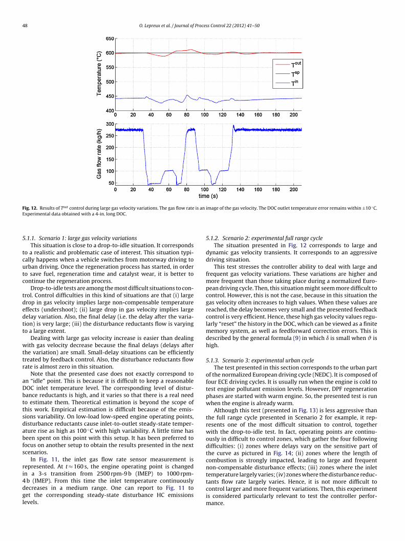
Fig. 12. Results of Tout control during large gas velocity variations. The gas flow rate is an image of the gas velocity. The DOC outlet temperature error remains within ±10 ◦C.E
5
tcutc
tdedtt
wttr
aDbttsdabfs
ri4dgl
xperimental data obtained with a 4-in. long DOC.
.1.1. Scenario 1: large gas velocity variationsThis situation is close to a drop-to-idle situation. It corresponds
o a realistic and problematic case of interest. This situation typi-ally happens when a vehicle switches from motorway driving torban driving. Once the regeneration process has started, in ordero save fuel, regeneration time and catalyst wear, it is better toontinue the regeneration process.
Drop-to-idle tests are among the most difficult situations to con-rol. Control difficulties in this kind of situations are that (i) largerop in gas velocity implies large non-compensable temperatureffects (undershoot); (ii) large drop in gas velocity implies largeelay variation. Also, the final delay (i.e. the delay after the varia-ion) is very large; (iii) the disturbance reductants flow is varyingo a large extent.
Dealing with large gas velocity increase is easier than dealingith gas velocity decrease because the final delays (delays after
he variation) are small. Small-delay situations can be efficientlyreated by feedback control. Also, the disturbance reductants flowate is almost zero in this situation.
Note that the presented case does not exactly correspond ton “idle” point. This is because it is difficult to keep a reasonableOC inlet temperature level. The corresponding level of distur-ance reductants is high, and it varies so that there is a real needo estimate them. Theoretical estimation is beyond the scope ofhis work. Empirical estimation is difficult because of the emis-ions variability. On low-load low-speed engine operating points,isturbance reductants cause inlet-to-outlet steady-state temper-ture rise as high as 100 ◦C with high variability. A little time haseen spent on this point with this setup. It has been preferred toocus on another setup to obtain the results presented in the nextcenarios.
In Fig. 11, the inlet gas flow rate sensor measurement isepresented. At t ≈ 160 s, the engine operating point is changedn a 3-s transition from 2500 rpm-9 b (IMEP) to 1000 rpm-
b (IMEP). From this time the inlet temperature continuouslyecreases in a medium range. One can report to Fig. 11 toet the corresponding steady-state disturbance HC emissionsevels.
5.1.2. Scenario 2: experimental full range cycleThe situation presented in Fig. 12 corresponds to large and
dynamic gas velocity transients. It corresponds to an aggressivedriving situation.
This test stresses the controller ability to deal with large andfrequent gas velocity variations. These variations are higher andmore frequent than those taking place during a normalized Euro-pean driving cycle. Then, this situation might seem more difficult tocontrol. However, this is not the case, because in this situation thegas velocity often increases to high values. When these values arereached, the delay becomes very small and the presented feedbackcontrol is very efficient. Hence, these high gas velocity values regu-larly “reset” the history in the DOC, which can be viewed as a finitememory system, as well as feedforward correction errors. This isdescribed by the general formula (9) in which ı is small when ϑ ishigh.
5.1.3. Scenario 3: experimental urban cycleThe test presented in this section corresponds to the urban part
of the normalized European driving cycle (NEDC). It is composed offour ECE driving cycles. It is usually run when the engine is cold totest engine pollutant emission levels. However, DPF regenerationphases are started with warm engine. So, the presented test is runwhen the engine is already warm.
Although this test (presented in Fig. 13) is less aggressive thanthe full range cycle presented in Scenario 2 for example, it rep-resents one of the most difficult situation to control, togetherwith the drop-to-idle test. In fact, operating points are continu-ously in difficult to control zones, which gather the four followingdifficulties: (i) zones where delays vary on the sensitive part ofthe curve as pictured in Fig. 14; (ii) zones where the length ofcombustion is strongly impacted, leading to large and frequentnon-compensable disturbance effects; (iii) zones where the inlettemperature largely varies; (iv) zones where the disturbance reduc-
tants flow rate largely varies. Hence, it is not more difficult tocontrol larger and more frequent variations. Then, this experimentis considered particularly relevant to test the controller perfor-mance.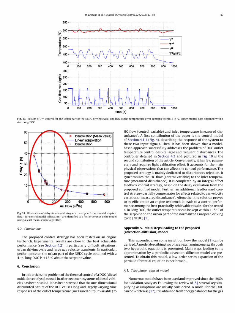
O. Lepreux et al. / Journal of Process Control 22 (2012) 41– 50 49
Fig. 13. Results of Tout control for the urban part of the NEDC driving cycle. The DOC ou4-in. long DOC.
Fdu
5
tpup4
6
ocdr
ig. 14. Illustration of delays involved during an urban cycle. Experimental step testata – for control model calibration – are identified to a first order plus delay modelsing a least mean-square algorithm.
.2. Conclusions
The proposed control strategy has been tested on an engineestbench. Experimental results are close to the best achievableerformance (see Section 4.2) in particularly difficult situations:rban driving cycle and large gas velocity transients. In particular,erformance on the urban part of the NEDC cycle obtained with a-in. long DOC is ±15 ◦C about the setpoint value.
. Conclusion
In this article, the problem of the thermal control of a DOC (diesel
xidation catalyst) as used in aftertreatment systems of diesel vehi-les has been studied. It has been stressed that the one-dimensionalistributed nature of the DOC causes long and largely varying timeesponses of the outlet temperature (measured output variable) totlet temperature error remains within ±15 ◦C. Experimental data obtained with a
HC flow (control variable) and inlet temperature (measured dis-turbance). A first contribution of the paper is the control modelof Section 4.1.1 (Fig. 4), describing the response of the system tothese two input signals. Then, it has been shown that a model-based approach successfully addresses the problem of DOC outlettemperature control despite large and frequent disturbances. Thecontroller detailed in Section 4.3 and pictured in Fig. 10 is thesecond contribution of the article. Conveniently, it has few param-eters and requires light calibration effort. It accounts for the mainphysical observations that can affect the control performance. Theproposed strategy is mainly dedicated to disturbances rejection. Itsynchronizes the HC flow (control variable) to the inlet tempera-ture (measured disturbance). It is completed by an integral effectfeedback control strategy, based on the delay evaluation from theproposed control model. Further, an additional feedforward con-trol strategy partially compensates for effects related to gas velocityvariations (measured disturbance). Altogether, the solution provesto be efficient on an engine testbench. It leads to a control perfor-mance among the best practically achievable results: for the tested4-in. long DOC, the outlet temperature can be kept within ±15 ◦C ofthe setpoint on the urban part of the normalized European drivingcycle (NEDC) [1].
Appendix A. Main steps leading to the proposed(advection-diffusion) model
This appendix gives some insight on how the model (1) can bederived. A model describing two phases exchanging energy throughtwo hyperbolic equations is presented. Main steps leading to itsapproximation by a parabolic advection-diffusion model are pre-sented. To obtain this model, a low-order series expansion of thepartial differential equation is performed.
A.1. Two-phase reduced model
Numerous models have been used and improved since the 1960sfor oxidation catalysts. Following the review of [5], several key sim-plifying assumptions are usually considered. A model for the DOCcan be written as (17). It is obtained from energy balances for the gas
5 Proce
ah⎧⎪⎪⎪⎪⎪⎪⎪⎨⎪⎪⎪⎪⎪⎪⎪⎩Tgg(catont
ebnnipb{
Etstbmbtr⎧⎪⎨⎪⎩ww⎧⎪⎪⎪⎪⎪⎨⎪⎪⎪⎪⎪⎩A
rt(
[
[
Control of Chemical Processes, Istanbul, Turkey, 2009.
0 O. Lepreux et al. / Journal of
nd the solid phases. Corresponding assumptions will be describedereafter.
εgCp∂T∂t
(z, t)︸ ︷︷ ︸Gas storage term
+ F(t)Acell
Cp∂T∂z
(z, t)︸ ︷︷ ︸Advection term
= −hgGa (T(z, t) − Ts(z, t))︸ ︷︷ ︸Convection term
(1 − ε)sCps∂Ts∂t
(z, t)︸ ︷︷ ︸Solid storage term
= hgGa (T(z, t) − Ts(z, t))︸ ︷︷ ︸Convection term
+ Gca
NM∑j=1
Rj(t) · hj
︸ ︷︷ ︸Heat source term
and Ts are the gas and monolith temperature, g and s are theas and monolith densities, Cp and Cps are the specific heat of theas and of the monolith, ε is the ratio of gas volume to total volumevoid ratio), Acell is the mean cell cross-sectional area (wall andhannel), hg is the convective heat transfer coefficient between gasnd solid, Ga is the geometric surface area-to-volume ratio, Gca ishe catalytic surface area-to-volume ratio, Rj is the rate of reactionf species j, hj is the enthalpy of chemical species j, and NM is theumber of considered species. For more details on these variables,he reader can refer to [5].
In the proposed model of Section 3.1 (dedicated to DPF regen-ration), several assumptions are made: the DOC is supposed toe thermally isolated and heat losses to the surroundings areeglected, axial diffusion in the fluid and solid phases can beeglected, the Nusselt and Sherwood numbers [12] (respectively,
ncluded in hg and Rj) can be assumed constant. Further, in the pro-osed model, the source term is lumped into a function � definedy
� (z, u(t), v(t)) = (u(t), v(t)), 0 ≤ z ≤ Lc(v(t))
� (z, u(t), v(t)) = 0, Lc(v(t)) < z ≤ L(18)
xothermic reactions are lumped into a single source term, dis-urbance reductants are considered separately from this term, theource term is independent of catalyst temperature, chemical andhermal dynamics are decoupled, � (z, u(t), v(t)) can be describedy a uniform profile as stated by (18), the reactive length Lc can beodeled as a function of variable v only, and temperature rise can
e expressed as a function of the gas velocity only. More details onhese assumptions can be found in [7]. Then, the model (17) can beewritten as
∂T∂t
(z, t) + v(t)∂T∂z
(z, t) = −k1(T(z, t) − Ts(z, t))
∂Ts∂t
(z, t) = k2(T(z, t) − Ts(z, t)) + � (z, u(t), v(t))
(19)
here parameters can be related to the physical parameters in (17)ith
k1 = hgGaεgCp
k2 = hgGa(1 − ε)sCps
v(t) = F(t)gεAcell
= F(t)gA0
(20)
.2. Advection-diffusion equation approximation
In (19), neglecting the gas thermal storage term ∂T/∂ t (which is aeasonable assumption), derivating the first equation with respecto t, and substituting Ts and ∂Ts/∂ t in the second equation leads to
not considering the source term here)∂T(z, t)∂t
+ ϑ∂T(z, t)∂z
+ �
ϑ
∂2T(z, t)∂t∂z
= 0 (21)
[[
ss Control 22 (2012) 41– 50
(17)
Following [13], T is expanded in the series (when ε � �/ϑ = v/k1is small) T = T0 + εTε + ε2Tε2 + . . ., where T0 is the solution of thefollowing advection equation
∂T0(z, t)∂t
+ ϑ∂T0(z, t)∂z
= 0 (22)
On one hand, expanding solutions of T in ε for (21) leads to
ε∂2T0
∂t∂z+ ε∂Tε∂t
+ ϑε∂Tε∂z
+ ε2 ∂2Tε
∂t∂z+ . . . = 0
On the other hand, expanding solutions of T in εfor the advection-diffusion equation (∂ T(z,t)/∂ t) + ϑ(∂ T(z,t)/∂ z) = �(∂ 2T(z, t)/∂ z2) leads to
ε∂2T0
∂t∂z+ ε∂Tε∂t
+ ϑε∂Tε∂z
− ε2ϑ∂2Tε∂z2
+ . . . = 0
So, expanding solutions of T in ε for (21) and for the advection-diffusion equation leads to the same equations up to order 1 in ε,i.e. T0 and Tε are the same in both cases. In this way they are simi-lar: their asymptotic expansions are equal up to order 1 (included)(see [7,13] for further calculation details). Considering these resultsyields the model (1).
Another way to proceed to highlight the relationship betweenthe two partial differential equations is as follows. Successively, onecan differentiate the simple cascade of partial differential equationsobtained for each term T0, Tε,. . .by matching powers of ε. A summa-tion of those differential relations makes the sought-after diffusionequation appear, along with a (distributed) source term, taking theform of a series, whose magnitude is ε3, which, again, suggests thatthe two equations are indeed closely related.
References
[1] Ecopoint Inc., DieselNet, Available online: http://www.dieselnet.com/.[2] E. Bisset, Mathematical model of the thermal regeneration of a wall-flow mono-
lith diesel particulate filter, Chem. Eng. Sci. 39 (1984) 1232–1244.[3] L. Achour, Dynamique et contrôle de la régénération d’un filtre à particules
diesel, Ph.D. Thesis, École des Mines de Paris—MINES ParisTech (2001).[4] G. Koltsakis, A. Stamatelos, Catalytic automotive exhaust aftertreatment, Prog.
Energy Combust. Sci. 23 (1997) 1–39.[5] C. Depcik, D. Assanis, One-dimensional automotive catalyst modeling, Prog.
Energy Combust. Sci. 31 (2005) 308–369.[6] S. Oh, J. Cavendish, Transients of monolithic catalytic converters: response to
step changes in feedstream temperature as related to controlling automobileemissions, Ind. Eng. Chem. 21 (1982) 29–37.
[7] O. Lepreux, Model-based temperature control of a diesel oxidation catalyst,Ph.D. Thesis, École des Mines de Paris—MINES ParisTech (2009).
[8] A. Frobert, Y. Creff, O. Lepreux, L. Schmidt, S. Raux, Generating thermal con-ditions to regenerate a DPF: impact of the reductant on the performances ofdiesel oxidation catalysts, SAE Paper 2009-01-1085, April 2009.
[9] O. Lepreux, Y. Creff, N. Petit, Practical achievable performance in diesel oxi-dation catalyst temperature control, Oil Gas Sci. Technol.–Rev. IFP Energiesnouvelles 66 (2011) 693–704.
10] J.R. Cannon, The One-dimensional Heat Equation, Vol. 23 of Encyclopedia ofMathematics and its Applications, Addison-Wesley Publishing Company, 1984.
11] O. Lepreux, Y. Creff, N. Petit, Model-based control design of a diesel oxidationcatalyst, in: Proc. of ADCHEM 2009, International Symposium on Advanced
12] M.N. Osizik, Basic Heat Transfer, McGraw-Hill, 1977.13] A.M. Il’in, The exponential boundary layer, in: M.V. Fedoryuk (Ed.), Partial Dif-
ferential Equations V: Asymptotic Methods for Partial Differential Equations,Springer-Verlag, 1998 (Section V.1).