Embed Size (px)
Citation preview
at SciVerse ScienceDirect
Journal of Power Sources 239 (2013) 253e264
Contents lists available
Journal of Power Sources
journal homepage: www.elsevier .com/locate/ jpowsour
Prognostics of lithium-ion batteries based on relevance vectors and aconditional three-parameter capacity degradation model
Dong Wang a, Qiang Miao b,*, Michael Pecht c
aDepartment of Systems Engineering & Engineering Management, City University of Hong Kong, Tat Chee Avenue, Kowloon, Hong Kong, Chinab School of Mechanical, Electronic and Industrial Engineering, University of Electronic Science and Technology of China, Chengdu, Sichuan 611731, ChinacCenter for Advanced Life Cycle Engineering (CALCE), University of Maryland, College Park, MD 20742, USA
h i g h l i g h t s
� Capacity degradation data are fitted by relevance vector machine.� Relevance vectors are used to find representative training vectors.� Representative training vectors are fitted by a conditional three-parameter capacity degradation model.� The developed model consists of an exponential function and a power function.� The remaining useful life of lithium-ion batteries is estimated.
a r t i c l e i n f o
Article history:Received 16 November 2012Received in revised form21 March 2013Accepted 23 March 2013Available online 2 April 2013
Keywords:Lithium-ion batteriesState of healthRemaining useful lifeRelevance vector machineBattery capacity degradation model
* Corresponding author.E-mail addresses: [email protected] (D. W
(Q. Miao), [email protected] (M. Pecht).
0378-7753/$ e see front matter � 2013 Elsevier B.V.http://dx.doi.org/10.1016/j.jpowsour.2013.03.129
a b s t r a c t
Lithium-ion batteries are widely used as power sources in commercial products, such as laptops, electricvehicles (EVs) and unmanned aerial vehicles (UAVs). In order to ensure a continuous power supply, thefunctionality and reliability of lithium-ion batteries have received considerable attention. In this paper, abattery capacity prognostic method is developed to estimate the remaining useful life of lithium-ionbatteries. This capacity prognostic method consists of a relevance vector machine and a conditionalthree-parameter capacity degradation model. The relevance vector machine is used to derive the rele-vance vectors that can be used to find the representative training vectors containing the cycles of therelevance vectors and the predictive values at the cycles of the relevance vectors. The conditional three-parameter capacity degradation model is developed to fit the predictive values at the cycles of therelevance vectors. Extrapolation of the conditional three-parameter capacity degradation model to afailure threshold is used to estimate the remaining useful life of lithium-ion batteries. Three instancestudies were conducted to validate the developed method. The results show that the developed methodis able to predict the future health condition of lithium-ion batteries.
� 2013 Elsevier B.V. All rights reserved.
1. Introduction
Prognostics is an enabling discipline that predicts the timewhena component or system will no longer satisfy its functionalityrequirement in its actual life cycle conditions [1e4]. It estimates theremaining useful life of the component or system [5], whereremaining useful life (RUL) [6] is defined as the period from thecurrent time until the system or component fails. Estimation of theRUL is used to conduct maintenance activities, provide spare partsin a timely manner, and prevent accidents.
ang), [email protected]
All rights reserved.
In recent years, lithium-ion batteries have become the mostcommon power supply for providing portable electronics andelectric vehicles (EVs)with electric energy [7]. However, lithium-ionbattery functionality gradually deteriorates over time. Failures oflithium-ion batteries result in economic and operational losses andcan have catastrophic consequences. In order to evaluate the per-formance of a lithium-ion battery, state of charge (SOC) and state ofhealth (SOH) estimation techniques are often implemented inlithium-ion battery management systems (BMSs) [7]. SOC is thepercentage of the remaining charge to the battery’s maximum ca-pacity until the lithium-ion battery needs to be recharged. SOHdescribes the physical health condition of a battery compared to afresh battery. The gradual decrease in the capacity of lithium-ionbatteries is a health indicator that tracks the degradation oflithium-ion batteries. Lithium-ion battery failures occur when the
D. Wang et al. / Journal of Power Sources 239 (2013) 253e264254
capacity degradation data of the lithium-ion battery drops belowsome percentage of its nominal capacity [8]. The failure threshold isrecommended to be around 80% of the rated value because the ca-pacity degradation data exhibit a trendwith exponential decay aftercrossing the 80% threshold [9]. Therefore, at the exponential decay,lithium-ion batteries become unreliable and should be replaced.
Yoshida et al. [10] investigated the capacity loss mechanism oflarge capacity lithium-ion cells for satellite application and devel-oped a simple life estimation model to fit the capacity loss data. Intheir subsequent work [11], they revised their previously devel-oped model by considering solid electrolyte interface growthblocking mechanism. The results showed that the revised modelcan be used to better fit ten-year long-term capacity loss data.Burgess [12] divided the float service life of a battery into twophases. During the first phase, the capacity loss was small. Thecapacity loss increased once the second phase began. A Kalmanfilter was applied to estimate the remaining float service life of avalve-regulated lead acid battery once the second phase began.However, the battery capacity fade in the second phasewas so shortthat an early failure alarm could not be triggered by this approach.He et al. [13] developed a lithium-ion battery prognostic method bycombining DempstereShafer theory (DST) and the Bayesian MonteCarlo (BMC) method. In their research, the sum of two exponentialfunctions was developed as a capacity degradation model, and DSTwas employed to estimate the initial values of this model. BMC wasthen adopted to infer the RUL. The advantage of this approach wasthat it was capable of providing an RUL prediction early in thebattery life. However, this method needed historical samples toprovide initial model parameters across the population of batteries.
Relevance vector machines (RVMs) [14] are gaining attention inprognostics. An RVM offers good generalization performance inregression and the sparse inferred predictors which are significantpredictors corresponding to a few non-zero weight parametersused in a regression function. Saha et al. [15,16] employed a rele-vance vector machine in a regression to fit the capacity degradationdata of lithium-ion batteries. They then used several differentparticle filters, such as a standard particle filter and a Rao-Blackwellized particle filter, to predict the RUL of the batteries.Their RVM and particle filter framework have been experimentallyproven to have advantages, such as reducing the prediction un-certainty, over autoregressive integrated moving average andextended Kalman filtering [17]. Widodo et al. [18] employed sampleentropy as a battery health indicator. A support vector machine anda RVM were used to predict the battery health condition. The re-sults showed that a relevance vector machine that is integratedwith sample entropy handles prediction uncertainty better than asupport vector machinewith the sample entropy. Caesarendra et al.[19] used kurtosis, which was the fourth standardized moment, tomeasure the peakedness of the non-stationary transient signalscaused by bearing localized faults and then employed logisticregression, which is a regression analysis method used for quan-titatively predicting a categorical variable based on one or morepredictor variables, to transform the kurtosis of bearing vibrationdegradation signals into bearing failure probability. The inputs andtarget vectors used for training RVM were kurtosis and bearingfailure probability, respectively. Then, the trained RVM wasemployed to track the bearing failure probability of unknown in-puts. Maio et al. [20] combined a relevance vector machine and anexponential function to estimate the remaining useful life ofbearings. Based on a similar idea, Zio and Maio [21] employed arelevance vector machine to find the most representative relevancevectors to fit a crack growth model for predicting remaining usefullife.
In this paper, a relevance vector machine is applied to get therelevance vectors used for finding the representative training
vectors. A comparison is done to show that the four parameters ofthe capacity degradation model in Ref. [13] cannot be uniquelydetermined with the representative training vectors. In order toobtain unique degradation model parameters, a conditional three-parameter capacity degradation model is developed to fit therepresentative training vectors. Extrapolation of the conditionalthree-parameter capacity degradation model to a failure thresholdis used to estimate the remaining useful life of lithium-ionbatteries.
The rest of this paper is organized as follows. In Section 2, therelevance vector machine is introduced. The battery prognosticmethod is developed in Section 3. Three instances are investigatedin Section 4 to validate the developed method for estimating theremaining useful life of lithium-ion batteries. Conclusions are dis-cussed in Section 5.
2. Brief introduction of relevance vector machine
This section introduces the relevant vector machine that is usedin this research. The general regression problem is discussed, andthe relevant vector machine and sparse Bayesian learning arepresented.
2.1. General regression problem
Given some target measurements y ¼ (y1,y2,.,yN)T and someinputs x¼ (x1,x2,.,xN), the general regression relationship betweenthe target and input vectors can be described by a model f(xi) withthe addition of noise 3i [22]:
yi ¼ f ðxiÞ þ 3i; i ¼ 1;2;.;N; (1)
where f(xi) is a linear combination of some known basis functionsfj(xi). The mathematical formula of f(xi) is given as:
f ðxiÞ ¼XMj¼1
wjfjðxiÞ ¼ fðxiÞw; (2)
where w ¼ (w1,w2,.,wM)T is a weight vector, andf(xi) ¼ (f1(xi),f2(xi),.,fM(xi)). The matrix form of Equation (1) iswritten as:
y ¼ Fw þ 3; (3)
whereF is anN�M designmatrix, whose j-th column consists ofNbasis functions fj(xi),i ¼ 1,2,.,N, and 3is a noise vector. Assumingthat each element of the noise vector is subject to the independentGaussian distribution with zero mean and variance s2, the likeli-hood of the complete training data set and the least square estimatewLS for the weight vector are given by[22]:
p�y���w; s2
�¼
�2ps2
��N=2exp
�� 12s2
���t�Fw���2
�(4)
wLS ¼ argminw
����t �Fw���2� ¼
�F
TF��1
FTy (5)
It should be noted that, in many cases, the matrix FTF is
frequently ill-conditioned, resulting in the estimate wLS sufferingfrom over-fitting and reducing predictive performance.
2.2. Relevance vector machine and sparse Bayesian learning
Relevance vector machine (RVM) is a special sparse linearmodel which has a form similar to a support vector machine
D. Wang et al. / Journal of Power Sources 239 (2013) 253e264 255
(SVM). SVM calculates predictions by using the following function[14]:
f ðxiÞ ¼XNj¼1
wjKj�xi; xj
þw0 ¼ FðxiÞw (6)
where Kj(xi,xj) is a kernel function, F(xi) ¼ [1,K(xi,x1),K(xi,x2),.,K(xi,xN)], and w ¼ (w0,w1,.,wN)T. The relevancevector machine is a Bayesian treatment of Equation (6). The kernelfunction used in the relevance vector machine does not need tosatisfy Mercer’s condition. Mercer’s condition is used to judgewhether a kernel is symmetric positive semi-definite and is the dotproduct of two mapping functions in some Euclidean space. It canavoid computing themapping function explicitly and use the kernelfunction instead [23]. However, in many cases, fulfilling Mercer’scondition is mathematically intractable. Because of the distributionassumption of the additive noise mentioned in Section 2.1, thelikelihood of the complete training data set is written as:
p�y���w; s2
�¼
�2ps2
��N=2exp
�� 12s2
kt�Fwk2�
(7)
whereF ¼ [f(x1),f(x2),.,f(xN)]T is a N � (Nþ1) design matrix, andf(xi) ¼ [1,K(xi,x1),K(xi,x2),.,K(xi,xN)]T. In order to avoid the severeover-fitting problem caused by themaximum likelihood estimationof the weight vector, a Bayesian method and imposed additionalconstraint parameters can be adopted. Define a zero-meanGaussian prior distribution over w [14]:
pðwjaÞ ¼YNi¼0
N�wij0;a�1
i
�(8)
where a ¼ (a0,a1,.,aN) is a vector consisting of Nþ1 hyper-parameters. Moreover, an individual hyperparameter is indepen-dently associated with each weight. A Gamma prior distribution isconducted on the hyperparameters and the noise variance s2 [14]:
pðaÞ ¼YNi¼0
Gammaðaija;bÞ (9)
pðbÞ ¼ Gammaðbjc;dÞ (10)
where bhs�2, and Gammaðaija;bÞ ¼ ðRN0 ta�1e�tdtÞ�1baaa�1e�ba.
When a, b, c, and d are set to zero, uniform hyperpriors over alogarithmic scale are formed.
Given the above prior assumptions and the training data, theposterior over all unknown parameters is given by Ref. [14]:
p�w;a; s2jy
�¼ p
�y��w;a; s2
p�w;a; s2
pðyÞ (11)
The posterior shown in Equation (11) cannot be directly calcu-lated and the integral of the denominator cannot be calculatedeither. In order to solve this problem, the posterior is reformulatedas [14]:
p�w;a; s2jy
�¼ p
�w���y;a; s2�p�a; s2jy� (12)
The posterior distribution over the weight vector is given by[14]:
p�w���y;a; s2� ¼ p
�y��w;s2
pðwjaÞ� �� 2
p y a; s
¼ ð2pÞ�ðNþ1Þ=2jSj�1=2
� exp��1
2ðw � mÞTS�1ðw � mÞ
� (13)
where S ¼ (s�2FTFþA)�1, m ¼ s�2SFTy and A ¼ diag(a0,a1,.,aN).The posterior distribution over the weight vector can be analyti-cally calculated, since pðyja; s2Þ ¼ R
pðyjw; s2ÞpðwjaÞdw is aconvolution of Gaussians. The second term on the right of Equation(12) is decomposed into [14]:
p�a; s2jy
�fp
�y���a; s2�pðaÞp�s2
�(14)
Because of the uniform hyperpriors assumption of p(a) andp(s2), Equation (14) becomes maximizing p(yja,s2) with respect toa and b. The formula of the marginal likelihood is given as [14]:
p�y���a; s2� ¼ð2pÞ�N=2
���s2IþFA�1FT����1=2
� exp�� 12tT�s2IþFA�1FT
�t�:
(15)
An iterative re-estimation method was introduced in [14] toobtain the values of aMP and s2MP that can maximize Equation (15),because the values of aMP and s2MP cannot be directly derived inclosed form. Meanwhile, in practice, many elements of the vectora ¼ (a0,a1,.,aN) tend to infinity during the iterative re-estimationprocedure. The posterior distribution over the correspondingweights shown in Equation (13) tend to be subject to a normaldistribution, N(0,0). In other words, p(wijy,a,s2) is highly concen-trated around zero. Additionally, many useless basis functions arepruned from the designmatrixF during the iterative re-estimationprocedure. As a result, relevance vectors are those training samplesthat correspond to the remaining non-zero weights. This definitionis analogous to the definition of support vectors. Support vectorscorrespond to the samples on the margin. At last, given a new inputx* and the values of aMP and s2MP, the predictive distribution overthe estimated measurement y* for the new input x* is given as [14]:
p�y*���y;aMP; s
2MP
�¼
Zp�y*���w;s2MP
�p�w���y;aMP; s
2MP
�
¼ N�y*jf*;s2*
�; (16)
where f* ¼ mTf(x*) and s2* ¼ s2MP þ fðx*ÞTSfðx*Þ. From Equation(16), the mean of the normal distribution can be treated as thepredictive value for the new input. The confidence of the predictivevalue is determined by the variance of this normal distribution.
3. Method for the estimation of remaining useful life oflithium-ion batteries
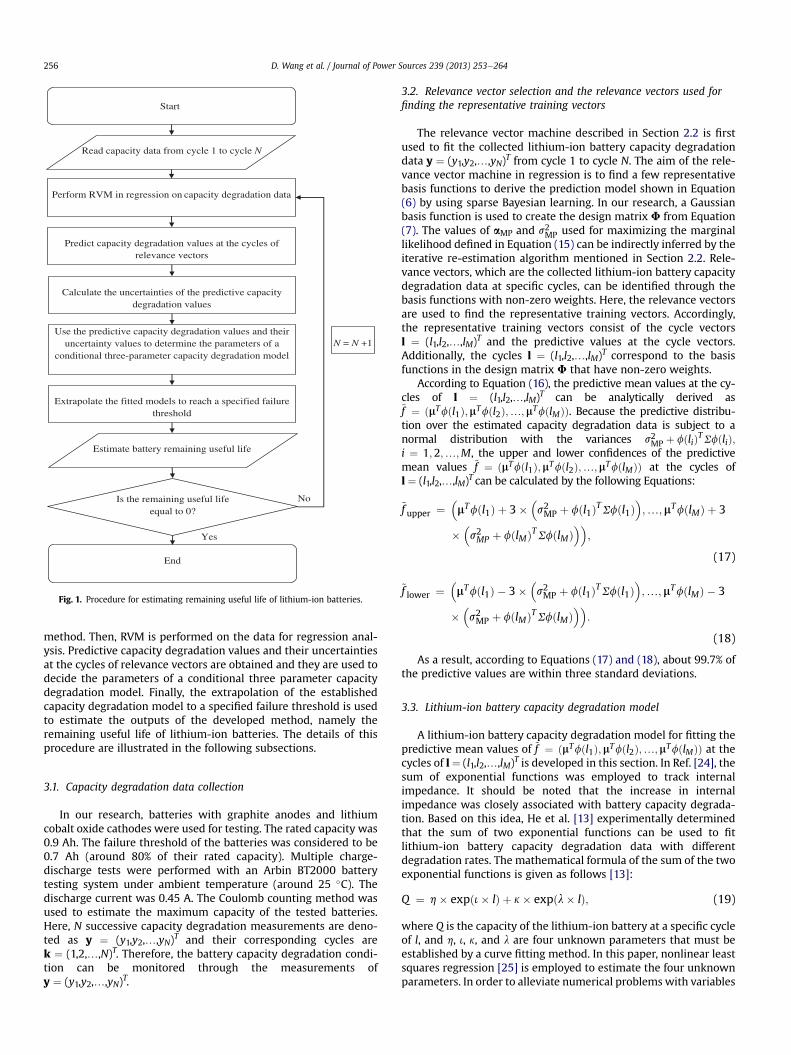
When a battery ages over time, its maximum capacity degradesto zero, indicating the deterioration of battery health. Estimation ofthe remaining maximum capacity ensures the reliability of a bat-tery for providing continuous power supplies to electronic equip-ment. Battery failure can be considered to occur once themaximumcapacity of the battery drops to 80% of its nominal value. Here, 80%is one of the typical examples suggested by reference [9] todetermine a specified failure threshold. In this paper, a batterycapacity prognostic method is developed to estimate the remaininguseful life of lithium-ion batteries. A flowchart of the battery ca-pacity prognostic procedure is shown in Fig. 1. First, the availablecapacity degradation data are used as the inputs for the developed
Perform RVM in regression on capacity degradation data
Predict capacity degradation values at the cycles ofrelevance vectors
Calculate the uncertainties of the predictive capacity degradation values
Use the predictive capacity degradation values and their uncertainty values to determine the parameters of a
conditional three-parameter capacity degradation model
Extrapolate the fitted models to reach a specified failure threshold
No
Yes
Start
End
Read capacity data from cycle 1 to cycle N
Estimate battery remaining useful life
N = N +1
Is the remaining useful life equal to 0?
Fig. 1. Procedure for estimating remaining useful life of lithium-ion batteries.
D. Wang et al. / Journal of Power Sources 239 (2013) 253e264256
method. Then, RVM is performed on the data for regression anal-ysis. Predictive capacity degradation values and their uncertaintiesat the cycles of relevance vectors are obtained and they are used todecide the parameters of a conditional three parameter capacitydegradation model. Finally, the extrapolation of the establishedcapacity degradation model to a specified failure threshold is usedto estimate the outputs of the developed method, namely theremaining useful life of lithium-ion batteries. The details of thisprocedure are illustrated in the following subsections.
3.1. Capacity degradation data collection
In our research, batteries with graphite anodes and lithiumcobalt oxide cathodes were used for testing. The rated capacity was0.9 Ah. The failure threshold of the batteries was considered to be0.7 Ah (around 80% of their rated capacity). Multiple charge-discharge tests were performed with an Arbin BT2000 batterytesting system under ambient temperature (around 25 �C). Thedischarge current was 0.45 A. The Coulomb counting method wasused to estimate the maximum capacity of the tested batteries.Here, N successive capacity degradation measurements are deno-ted as y ¼ (y1,y2,.,yN)T and their corresponding cycles arek ¼ (1,2,.,N)T. Therefore, the battery capacity degradation condi-tion can be monitored through the measurements ofy ¼ (y1,y2,.,yN)T.
3.2. Relevance vector selection and the relevance vectors used forfinding the representative training vectors
The relevance vector machine described in Section 2.2 is firstused to fit the collected lithium-ion battery capacity degradationdata y ¼ (y1,y2,.,yN)T from cycle 1 to cycle N. The aim of the rele-vance vector machine in regression is to find a few representativebasis functions to derive the prediction model shown in Equation(6) by using sparse Bayesian learning. In our research, a Gaussianbasis function is used to create the design matrix F from Equation(7). The values of aMP and s2MP used for maximizing the marginallikelihood defined in Equation (15) can be indirectly inferred by theiterative re-estimation algorithm mentioned in Section 2.2. Rele-vance vectors, which are the collected lithium-ion battery capacitydegradation data at specific cycles, can be identified through thebasis functions with non-zero weights. Here, the relevance vectorsare used to find the representative training vectors. Accordingly,the representative training vectors consist of the cycle vectorsl ¼ (l1,l2,.,lM)T and the predictive values at the cycle vectors.Additionally, the cycles l ¼ (l1,l2,.,lM)T correspond to the basisfunctions in the design matrix F that have non-zero weights.
According to Equation (16), the predictive mean values at the cy-cles of l ¼ (l1,l2,.,lM)T can be analytically derived as~f ¼ ðmTfðl1Þ;mTfðl2Þ;.;mTfðlMÞÞ. Because the predictive distribu-tion over the estimated capacity degradation data is subject to anormal distribution with the variances s2MP þ fðliÞTSfðliÞ;i ¼ 1;2;.;M, the upper and lower confidences of the predictivemean values ~f ¼ ðmTfðl1Þ;mTfðl2Þ;.;mTfðlMÞÞ at the cycles ofl ¼ (l1,l2,.,lM)T can be calculated by the following Equations:
~f upper ¼�mTfðl1Þ þ 3�
�s2MP þ fðl1ÞTSfðl1Þ
�;.;mTfðlMÞ þ 3
��s2MP þ fðlMÞTSfðlMÞ
��;
(17)
~f lower ¼�mTfðl1Þ � 3�
�s2MP þ fðl1ÞTSfðl1Þ
�;.;mTfðlMÞ � 3
��s2MP þ fðlMÞTSfðlMÞ
��:
(18)
As a result, according to Equations (17) and (18), about 99.7% ofthe predictive values are within three standard deviations.
3.3. Lithium-ion battery capacity degradation model
A lithium-ion battery capacity degradation model for fitting thepredictive mean values of ~f ¼ ðmTfðl1Þ;mTfðl2Þ;.;mTfðlMÞÞ at thecycles of l¼ (l1,l2,.,lM)T is developed in this section. In Ref. [24], thesum of exponential functions was employed to track internalimpedance. It should be noted that the increase in internalimpedance was closely associated with battery capacity degrada-tion. Based on this idea, He et al. [13] experimentally determinedthat the sum of two exponential functions can be used to fitlithium-ion battery capacity degradation data with differentdegradation rates. The mathematical formula of the sum of the twoexponential functions is given as follows [13]:
Q ¼ h� expði� lÞ þ k� expðl� lÞ; (19)
where Q is the capacity of the lithium-ion battery at a specific cycleof l, and h, i, k, and l are four unknown parameters that must beestablished by a curve fitting method. In this paper, nonlinear leastsquares regression [25] is employed to estimate the four unknownparameters. In order to alleviate numerical problems with variables
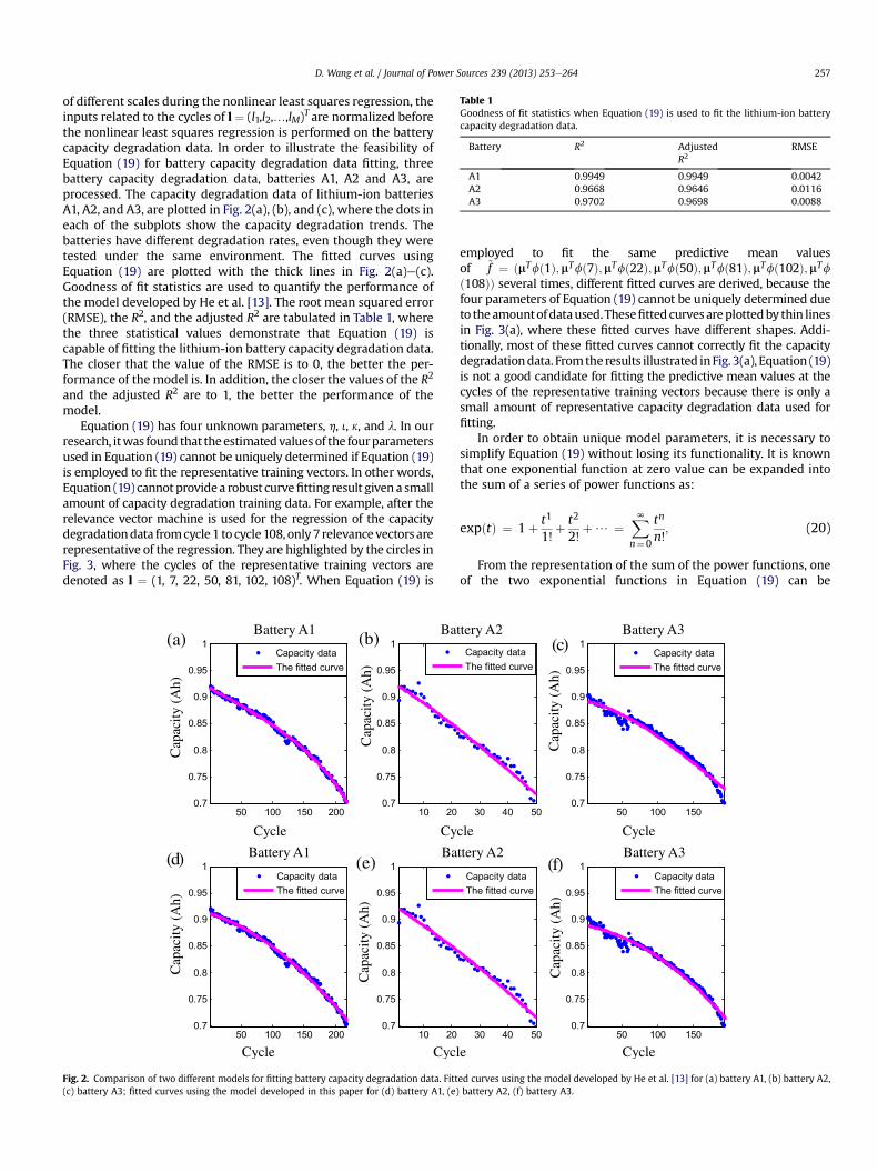
Table 1Goodness of fit statistics when Equation (19) is used to fit the lithium-ion batterycapacity degradation data.
Battery R2 AdjustedR2
RMSE
A1 0.9949 0.9949 0.0042A2 0.9668 0.9646 0.0116A3 0.9702 0.9698 0.0088
D. Wang et al. / Journal of Power Sources 239 (2013) 253e264 257
of different scales during the nonlinear least squares regression, theinputs related to the cycles of l ¼ (l1,l2,.,lM)T are normalized beforethe nonlinear least squares regression is performed on the batterycapacity degradation data. In order to illustrate the feasibility ofEquation (19) for battery capacity degradation data fitting, threebattery capacity degradation data, batteries A1, A2 and A3, areprocessed. The capacity degradation data of lithium-ion batteriesA1, A2, and A3, are plotted in Fig. 2(a), (b), and (c), where the dots ineach of the subplots show the capacity degradation trends. Thebatteries have different degradation rates, even though they weretested under the same environment. The fitted curves usingEquation (19) are plotted with the thick lines in Fig. 2(a)e(c).Goodness of fit statistics are used to quantify the performance ofthe model developed by He et al. [13]. The root mean squared error(RMSE), the R2, and the adjusted R2 are tabulated in Table 1, wherethe three statistical values demonstrate that Equation (19) iscapable of fitting the lithium-ion battery capacity degradation data.The closer that the value of the RMSE is to 0, the better the per-formance of the model is. In addition, the closer the values of the R2
and the adjusted R2 are to 1, the better the performance of themodel.
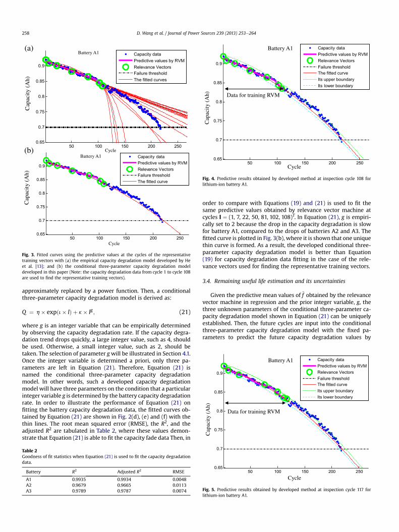
Equation (19) has four unknown parameters, h, i, k, and l. In ourresearch, itwas found that theestimatedvaluesof the fourparametersused in Equation (19) cannot be uniquely determined if Equation (19)is employed to fit the representative training vectors. In other words,Equation (19) cannot providea robust curvefitting result given a smallamount of capacity degradation training data. For example, after therelevance vector machine is used for the regression of the capacitydegradationdata fromcycle1 to cycle108, only7 relevancevectors arerepresentative of the regression. They are highlighted by the circles inFig. 3, where the cycles of the representative training vectors aredenoted as l ¼ (1, 7, 22, 50, 81, 102, 108)T. When Equation (19) is
50 100 150 2000.7
0.75
0.8
0.85
0.9
0.95
1
10 200.7
0.75
0.8
0.85
0.9
0.95
1
10 200.7
0.75
0.8
0.85
0.9
0.95
1Capacity dataThe fitted curve
50 100 150 2000.7
0.75
0.8
0.85
0.9
0.95
1Capacity dataThe fitted curve
Cap
acity
(A
h)C
apac
ity (
Ah)
Cycle
(a)
(d)
Cy
Cycle Cycl
Cap
acity
(A
h)
(b)
Cap
acity
(A
h)
(e)
Battery A1 Ba
Battery A1 Ba
Fig. 2. Comparison of two different models for fitting battery capacity degradation data. Fitt(c) battery A3; fitted curves using the model developed in this paper for (d) battery A1, (e)
employed to fit the same predictive mean valuesof ~f ¼ ðmTfð1Þ;mTfð7Þ;mTfð22Þ;mTfð50Þ;mTfð81Þ;mTfð102Þ;mTf
ð108ÞÞ several times, different fitted curves are derived, because thefour parameters of Equation (19) cannot be uniquely determined dueto theamountofdataused.Thesefittedcurves areplottedby thin linesin Fig. 3(a), where these fitted curves have different shapes. Addi-tionally, most of these fitted curves cannot correctly fit the capacitydegradationdata. Fromtheresults illustrated inFig. 3(a), Equation (19)is not a good candidate for fitting the predictive mean values at thecycles of the representative training vectors because there is only asmall amount of representative capacity degradation data used forfitting.
In order to obtain unique model parameters, it is necessary tosimplify Equation (19) without losing its functionality. It is knownthat one exponential function at zero value can be expanded intothe sum of a series of power functions as:
expðtÞ ¼ 1þ t1
1!þ t2
2!þ/ ¼
XNn¼0
tn
n!; (20)
From the representation of the sum of the power functions, oneof the two exponential functions in Equation (19) can be
30 40 50
30 40 50
50 100 1500.7
0.75
0.8
0.85
0.9
0.95
1
50 100 1500.7
0.75
0.8
0.85
0.9
0.95
1Capacity dataThe fitted curve
Capacity dataThe fitted curve
Capacity dataThe fitted curve
Capacity dataThe fitted curve
cle Cycle
e Cycle
Cap
acity
(A
h)
(c)
Cap
acity
(A
h)
(f)
ttery A2 Battery A3
ttery A2 Battery A3
ed curves using the model developed by He et al. [13] for (a) battery A1, (b) battery A2,battery A2, (f) battery A3.
50 100 150 200 2500.65
0.7
0.75
0.8
0.85
0.9
Capacity dataPredictive values by RVMRelevance VectorsFailure thresholdThe fitted curves
50 100 150 200 2500.65
0.7
0.75
0.8
0.85
0.9
Capacity dataPredictive values by RVMRelevance VectorsFailure thresholdThe fitted curve
Cap
acity
(A
h)
Cycle
Battery A1
Cycle
Cap
acity
(A
h)
Battery A1
(a)
(b)
Fig. 3. Fitted curves using the predictive values at the cycles of the representativetraining vectors with (a) the empirical capacity degradation model developed by Heet al. [13]; and (b) the conditional three-parameter capacity degradation modeldeveloped in this paper (Note: the capacity degradation data from cycle 1 to cycle 108are used to find the representative training vectors).
50 100 150 200 2500.65
0.7
0.75
0.8
0.85
0.9
Capacity dataPredictive values by RVMRelevance VectorsFailure thresholdThe fitted curveIts upper boundaryIts lower boundary
Cap
acity
(A
h)
Cycle
Battery A1
Data for training RVM
Fig. 4. Predictive results obtained by developed method at inspection cycle 108 forlithium-ion battery A1.
0.75
0.8
0.85
0.9
Capacity dataPredictive values by RVMRelevance VectorsFailure thresholdThe fitted curveIts upper boundaryIts lower boundary
Cap
acity
(A
h)
Battery A1
Data for training RVM
D. Wang et al. / Journal of Power Sources 239 (2013) 253e264258
approximately replaced by a power function. Then, a conditionalthree-parameter capacity degradation model is derived as:
Q ¼ h� expði� lÞ þ k� lg ; (21)
where g is an integer variable that can be empirically determinedby observing the capacity degradation rate. If the capacity degra-dation trend drops quickly, a large integer value, such as 4, shouldbe used. Otherwise, a small integer value, such as 2, should betaken. The selection of parameter gwill be illustrated in Section 4.1.Once the integer variable is determined a priori, only three pa-rameters are left in Equation (21). Therefore, Equation (21) isnamed the conditional three-parameter capacity degradationmodel. In other words, such a developed capacity degradationmodel will have three parameters on the condition that a particularinteger variable g is determined by the battery capacity degradationrate. In order to illustrate the performance of Equation (21) onfitting the battery capacity degradation data, the fitted curves ob-tained by Equation (21) are shown in Fig. 2(d), (e) and (f) with thethin lines. The root mean squared error (RMSE), the R2, and theadjusted R2 are tabulated in Table 2, where these values demon-strate that Equation (21) is able to fit the capacity fade data Then, in
Table 2Goodness of fit statistics when Equation (21) is used to fit the capacity degradationdata.
Battery R2 Adjusted R2 RMSE
A1 0.9935 0.9934 0.0048A2 0.9679 0.9665 0.0113A3 0.9789 0.9787 0.0074
order to compare with Equations (19) and (21) is used to fit thesame predictive values obtained by relevance vector machine atcycles l ¼ (1, 7, 22, 50, 81, 102, 108)T. In Equation (21), g is empiri-cally set to 2 because the drop in the capacity degradation is slowfor battery A1, compared to the drops of batteries A2 and A3. Thefitted curve is plotted in Fig. 3(b), where it is shown that one uniquethin curve is formed. As a result, the developed conditional three-parameter capacity degradation model is better than Equation(19) for capacity degradation data fitting in the case of the rele-vance vectors used for finding the representative training vectors.
3.4. Remaining useful life estimation and its uncertainties
Given the predictive mean values of ~f obtained by the relevancevector machine in regression and the prior integer variable, g, thethree unknown parameters of the conditional three-parameter ca-pacity degradation model shown in Equation (21) can be uniquelyestablished. Then, the future cycles are input into the conditionalthree-parameter capacity degradation model with the fixed pa-rameters to predict the future capacity degradation values by
50 100 150 200 2500.65
0.7
Cycle
Fig. 5. Predictive results obtained by developed method at inspection cycle 117 forlithium-ion battery A1.
50 100 150 200 2500.65
0.7
0.75
0.8
0.85
0.9
Capacity dataPredictive values by RVMRelevance VectorsFailure thresholdThe fitted curveIts upper boundaryIts lower boundary
Cap
acity
(A
h)
Cycle
Battery A1
Data for training RVM
Fig. 6. Predictive results obtained by developed method at inspection cycle 125 forlithium-ion battery A1.
50 100 150 200 2500.65
0.7
0.75
0.8
0.85
0.9
Capacity dataPredictive values by RVMRelevance VectorsFailure thresholdThe fitted curveIts upper boundaryIts lower boundary
Cap
acity
(A
h)
Cycle
Battery A1
Data for training RVM
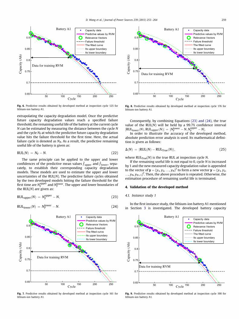
Fig. 8. Predictive results obtained by developed method at inspection cycle 176 forlithium-ion battery A1.
D. Wang et al. / Journal of Power Sources 239 (2013) 253e264 259
extrapolating the capacity degradation model. Once the predictivefuture capacity degradation values reach a specified failurethreshold, the remaining useful life of the battery at the current cycleN can be estimated by measuring the distance between the cycle Nand the cycle NF at which the predictive future capacity degradationvalue hits the failure threshold for the first time. Here, the actualfailure cycle is denoted as NA. As a result, the predictive remaininguseful life of the battery is given as:
RULðNÞ ¼ NF � N: (22)
The same principle can be applied to the upper and lowerconfidences of the predictive mean values ~f upper and ~f lower, sepa-rately, to establish their corresponding capacity degradationmodels. These models are used to estimate the upper and loweruncertainties of the RUL(N). The predictive failure cycles obtainedby the two developed models hitting the failure threshold for thefirst time are Nupper
F and NlowerF . The upper and lower boundaries of
the RUL(N) are given as:
RULupperðNÞ ¼ NupperF � N; (23)
RULlowerðNÞ ¼ NlowerF � N: (24)
50 100 150 200 2500.65
0.7
0.75
0.8
0.85
0.9
Capacity dataPredictive values by RVMRelevance VectorsFailure thresholdThe fitted curveIts upper boundaryIts lower boundary
Cap
acity
(A
h)
Cycle
Battery A1
Data for training RVM
Fig. 7. Predictive results obtained by developed method at inspection cycle 161 forlithium-ion battery A1.
Consequently, by combining Equations (23) and (24), the truevalue of the RUL(N) will be held by a 99.7% confidence interval½RULlowerðNÞ;RULupperðNÞ� ¼ ½Nlower
F � N;NupperF � N�.
In order to illustrate the accuracy of the developed method,absolute prediction error analysis is used. Its mathematical defini-tion is given as follows:
DðNÞ ¼ jRULðNÞ � RULTrueðNÞj; (25)
where RULTrue(N) is the true RUL at inspection cycle N.If the remaining useful life is not equal to 0, cycle N is increased
by 1 and the newmeasured capacity degradation value is appendedto the vector of y ¼ (y1, y2, ., yN)T to form a new vector y ¼ (y1, y2,., yN, yNþ1)T. Then, the above procedure is repeated. Otherwise, theestimation procedure of remaining useful life is terminated.
4. Validation of the developed method
4.1. Instance study 1
In the first instance study, the lithium-ion battery A1mentionedin Section 3 is investigated. The developed battery capacity
50 100 150 200 2500.65
0.7
0.75
0.8
0.85
0.9
Capacity dataPredictive values by RVMRelevance VectorsFailure thresholdThe fitted curveIts upper boundaryIts lower boundary
Cap
acity
(A
h)
Cycle
Battery A1
Data for training RVM
Fig. 9. Predictive results obtained by developed method at inspection cycle 190 forlithium-ion battery A1.
50 100 150 200 2500.65
0.7
0.75
0.8
0.85
0.9
Capacity dataPredictive values by RVMRelevance VectorsFailure thresholdThe fitted curveIts upper boundaryIts lower boundary
Cap
acity
(A
h)
Cycle
Battery A1
Data for training RVM
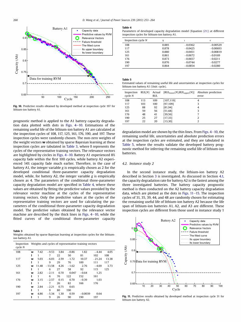
Fig. 10. Predictive results obtained by developed method at inspection cycle 197 forlithium-ion battery A1.
Table 4Parameters of developed capacity degradation model (Equation (21)) at differentinspection cycles for lithium-ion battery A1.
Inspection cycle N h i k
108 0.885 �0.0362 �0.00529117 0.878 �0.0425 �0.00693125 0.880 �0.0451 �0.00819161 0.861 �0.0672 �0.0169176 0.873 �0.0657 �0.0211190 0.876 �0.0744 �0.0277197 0.864 �0.0854 �0.0280
Table 5Estimated values of remaining useful life and uncertainties at inspection cycles forlithium-ion battery A1 (Unit: cycle).
Inspectioncycle N
RUL(N) ActualRUL
[RULlower(N),RULupper(N)] Absolute predictionerror
108 113 109 [107,119] 4117 103 100 [97,109] 3125 88 92 [81,94] 4161 59 56 [51,68] 3176 48 41 [39,56] 7190 25 27 [17,33] 2197 22 20 [13,30] 2
Battery A2
D. Wang et al. / Journal of Power Sources 239 (2013) 253e264260
prognostic method is applied to the A1 battery capacity degrada-tion data plotted with dots in Figs. 4e10. Estimations of theremaining useful life of the lithium-ion battery A1 are calculated atthe inspection cycles of 108, 117, 125, 161, 176, 190, and 197. Theseinspection cycles were randomly chosen. The non-zero weights ofthe weight vectorsw obtained by sparse Bayesian learning at theseinspection cycles are tabulated in Table 3, where l represents thecycles of the representative training vectors. The relevance vectorsare highlighted by circles in Figs. 4e10. Battery A1 experienced 8%capacity fade within the first 100 cycles, while battery A2 experi-enced 14% capacity fade much earlier. Therefore, in the case ofbattery A1, the integer variable g is empirically chosen as 2 for thedeveloped conditional three-parameter capacity degradationmodel, while, for battery A2, the integer variable g is empiricallychosen as 4. The parameters of the conditional three-parametercapacity degradation model are specified in Table 4, where thesevalues are obtained by fitting the predictive values provided by therelevance vector machine at the cycles of the representativetraining vectors. Only the predictive values at the cycles of therepresentative training vectors are used for calculating the pa-rameters of the conditional three-parameter capacity degradationmodel. The predictive values obtained by the relevance vectormachine are described by the thick lines in Figs. 4e10, while thefitted curves of the conditional three-parameter capacity
Table 3Weights obtained by sparse Bayesian learning at inspection cycles for the lithium-ion battery A1.
Inspectioncycle N
Weights and cycles of representative training vectors
108 w 7.42 �9.53 3.84 �0.86 1.82 �4.44 4.05l 1 7 22 50 81 102 108
117 w 5.03 �6.03 2.59 �1.72 10.37 �21.24 13.38l 1 9 29 76 100 111 117
125 w 11.48 �13.58 4.26 �1.62 2.76 �4.69 3.73l 1 6 27 58 92 115 125
161 w 2.82 �2.11 0.70 0.047 �0.64 1.25l 1 6 76 122 152 161
176 w 3.15 �2.57 0.15 0.70 �0.39 1.03l 1 7 26 82 166 176
190 w 2.84 �2.21 0.75 0.65l 1 9 80 190
197 w 4.86 �5.34 1.30 0.59 �0.0039 0.64l 1 9 26 90 190 197
degradationmodel are shown by the thin lines. From Figs. 4e10, theremaining useful life, uncertainties and absolute prediction errorsat the inspection cycles are estimated, and they are tabulated inTable 5, where the results validate the developed battery prog-nostic method for inferring the remaining useful life of lithium-ionbatteries.
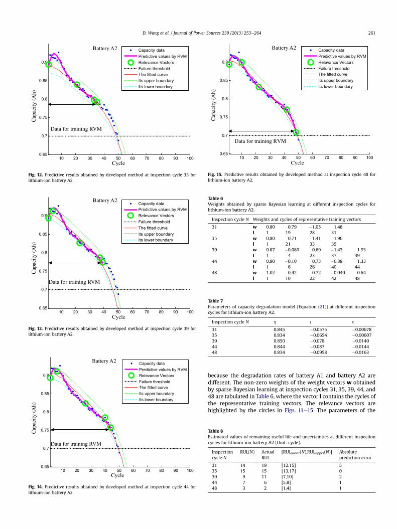
4.2. Instance study 2
In the second instance study, the lithium-ion battery A2described in Section 3 is investigated. As discussed in Section 4.1,the capacity degradation rate for battery A2 is the fastest among thethree investigated batteries. The battery capacity prognosticmethod is then conducted on the A2 battery capacity degradationdata, which are plotted as the dots in Figs. 11e15. The inspectioncycles of 31, 35, 39, 44, and 48 are randomly chosen for estimatingthe remaining useful life of lithium-ion battery A2 because the lifespan of lithium-ion batteries A1, A2, and A3 are different. Theseinspection cycles are different from those used in instance study 1
10 20 30 40 50 60 70 80 90 1000.65
0.7
0.75
0.8
0.85
0.9
Capacity dataPredictive values by RVMRelevance VectorsFailure thresholdThe fitted curveIts upper boundaryIts lower boundary
Cap
acity
(A
h)
Cycle
Data for training RVM
Fig. 11. Predictive results obtained by developed method at inspection cycle 31 forlithium-ion battery A2.
10 20 30 40 50 60 70 80 90 1000.65
0.7
0.75
0.8
0.85
0.9
Capacity dataPredictive values by RVMRelevance VectorsFailure thresholdThe fitted curveIts upper boundaryIts lower boundary
Cap
acity
(A
h)
Cycle
Battery A2
Data for training RVM
Fig. 12. Predictive results obtained by developed method at inspection cycle 35 forlithium-ion battery A2.
10 20 30 40 50 60 70 80 90 1000.65
0.7
0.75
0.8
0.85
0.9
Capacity dataPredictive values by RVMRelevance VectorsFailure thresholdThe fitted curveIts upper boundaryIts lower boundary
Cap
acity
(A
h)
Cycle
Battery A2
Data for training RVM
Fig. 13. Predictive results obtained by developed method at inspection cycle 39 forlithium-ion battery A2.
10 20 30 40 50 60 70 80 90 1000.65
0.7
0.75
0.8
0.85
0.9
Capacity dataPredictive values by RVMRelevance VectorsFailure thresholdThe fitted curveIts upper boundaryIts lower boundary
Cap
acity
(A
h)
Cycle
Battery A2
Data for training RVM
Fig. 14. Predictive results obtained by developed method at inspection cycle 44 forlithium-ion battery A2.
10 20 30 40 50 60 70 80 90 1000.65
0.7
0.75
0.8
0.85
0.9
Capacity dataPredictive values by RVMRelevance VectorsFailure thresholdThe fitted curveIts upper boundaryIts lower boundary
Cap
acity
(A
h)
Cycle
Battery A2
Data for training RVM
Fig. 15. Predictive results obtained by developed method at inspection cycle 48 forlithium-ion battery A2.
Table 6Weights obtained by sparse Bayesian learning at different inspection cycles forlithium-ion battery A2.
Inspection cycle N Weights and cycles of representative training vectors
31 w 0.80 0.79 �1.05 1.48l 1 19 28 31
35 w 0.80 0.71 �1.41 1.90l 1 21 33 35
39 w 0.87 �0.080 0.69 �1.43 1.93l 1 4 23 37 39
44 w 0.90 �0.10 0.73 �0.88 1.33l 1 6 26 40 44
48 w 1.02 �0.42 0.72 �0.040 0.64l 1 10 22 42 48
Table 7Parameters of capacity degradation model (Equation (21)) at different inspectioncycles for lithium-ion battery A2.
Inspection cycle N h i k
31 0.845 �0.0575 �0.0067835 0.834 �0.0654 �0.0060739 0.850 �0.078 �0.014044 0.844 �0.087 �0.014448 0.834 �0.0958 �0.0163
D. Wang et al. / Journal of Power Sources 239 (2013) 253e264 261
because the degradation rates of battery A1 and battery A2 aredifferent. The non-zero weights of the weight vectors w obtainedby sparse Bayesian learning at inspection cycles 31, 35, 39, 44, and48 are tabulated in Table 6, where the vector l contains the cycles ofthe representative training vectors. The relevance vectors arehighlighted by the circles in Figs. 11e15. The parameters of the
Table 8Estimated values of remaining useful life and uncertainties at different inspectioncycles for lithium-ion battery A2 (Unit: cycle).
Inspectioncycle N
RUL(N) ActualRUL
[RULlower(N),RULupper(N)] Absoluteprediction error
31 14 19 [12,15] 535 15 15 [13,17] 039 9 11 [7,10] 244 7 6 [5,8] 148 3 2 [1,4] 1
50 100 150 2000.65
0.7
0.75
0.8
0.85
0.9
Capacity dataPredictive values by RVMRelevance VectorsFailure thresholdThe fitted curveIts upper boundaryIts lower boundary
Cap
acity
(A
h)
Cycle
Battery A3
Data for training RVM
Fig. 16. Predictive results obtained by developed method at inspection cycle 104 forlithium-ion battery A3.
50 100 150 2000.65
0.7
0.75
0.8
0.85
0.9
Capacity dataPredictive values by RVMRelevance VectorsFailure thresholdThe fitted curveIts upper boundaryIts lower boundary
Cap
acity
(A
h)
Cycle
Battery A3
Data for training RVM
Fig. 17. Predictive results obtained by developed method at inspection cycle 128 forlithium-ion battery A3.
50 100 150 2000.65
0.7
0.75
0.8
0.85
0.9
Capacity dataPredictive values by RVMRelevance VectorsFailure thresholdThe fitted curveIts upper boundaryIts lower boundary
Cap
acity
(A
h)
Cycle
Battery A3
Data for training RVM
Fig. 18. Predictive results obtained by developed method at inspection cycle 146 forlithium-ion battery A3.
50 100 150 2000.65
0.7
0.75
0.8
0.85
0.9
Capacity dataPredictive values by RVMRelevance VectorsFailure thresholdThe fitted curveIts upper boundaryIts lower boundary
Cap
acity
(A
h)
Cycle
Battery A3
Data for training RVM
Fig. 19. Predictive results obtained by developed method at inspection cycle 157 forlithium-ion battery A3.
50 100 150 2000.65
0.7
0.75
0.8
0.85
0.9
Capacity dataPredictive values by RVMRelevance VectorsFailure thresholdThe fitted curveIts upper boundaryIts lower boundary
Cap
acity
(A
h)
Cycle
Battery A3
Data for training RVM
Fig. 20. Predictive results obtained by developed method at inspection cycle 170 forlithium-ion battery A3.
50 100 150 2000.65
0.7
0.75
0.8
0.85
0.9
Capacity dataPredictive values by RVMRelevance VectorsFailure thresholdThe fitted curveIts upper boundaryIts lower boundary
Cap
acity
(A
h)
Cycle
Battery A3
Data for training RVM
Fig. 21. Predictive results obtained by developed method at inspection cycle 183 forlithium-ion battery A3.
D. Wang et al. / Journal of Power Sources 239 (2013) 253e264262
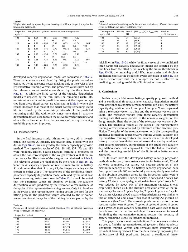
Table 9Weights obtained by sparse Bayesian learning at different inspection cycles forlithium-ion battery A3.
Inspectioncycle N
Weights and cycles of representative training vectors
104 w 1.54 �0.81 0.69 �0.68 1.32l 1 7 53 98 104
128 w 1.63 �0.90 0.39 0.33 �1.04 1.66l 1 8 65 68 122 128
146 w 1.84 �1.16 0.70 0.034 �0.60 1.23l 1 10 70 73 138 146
157 w 2.65 �1.96 0.72 �0.85 1.49l 1 7 74 152 157
170 w 7.01 �7.35 1.52 0.97 �3.09 3.07l 1 7 36 132 162 170
183 w 3.49 �3.06 0.25 0.70 0.64l 1 9 35 78 183
Table 11Estimated values of remaining useful life and uncertainties at different inspectioncycles for lithium-ion battery A3 (Unit: cycle).
The inspectioncycle of N
RUL(N) ActualRUL
[RULlower(N),RULupper(N)] Absoluteprediction error
104 82 91 [73,91] 9128 74 67 [65,87] 7146 45 49 [37,48] 4157 38 38 [35,48] 0170 33 25 [26,39] 8183 11 12 [5,17] 1
D. Wang et al. / Journal of Power Sources 239 (2013) 253e264 263
developed capacity degradation model are tabulated in Table 7.These parameters are calculated by fitting the predictive valuesestimated by the relevance vector machine only at the cycles of therepresentative training vectors. The predictive values provided bythe relevance vector machine are shown by the thick lines inFigs. 11e15, while the fitted curves of the capacity degradationmodel are depicted by the thin lines. The remaining useful life,uncertainties and absolute prediction errors at the inspection cy-cles from these fitted curves are tabulated in Table 8, where theresults illustrate that most of the actual battery remaining usefullife is covered by the uncertainty intervals of the predictedremaining useful life. Additionally, since more than 31 capacitydegradation data is used to train the relevance vector machine andobtain the relevance vectors, the accuracy of battery remaininguseful life prediction improves.
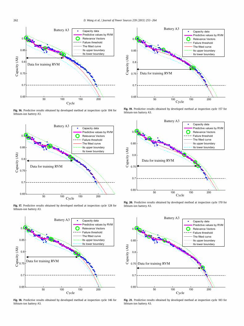
4.3. Instance study 3
In the final instance study, lithium-ion battery A3 is investi-gated. The battery A3 capacity degradation data, plotted with thedots in Figs. 16e21, are analyzed by the battery capacity prognosticmethod. The inspection cycles of 104, 128, 146, 157, 170, and 183were randomly chosen. Sparse Bayesian learning is employed toobtain the non-zero weights of the weight vectors w at these in-spection cycles. The values of the weights are tabulated in Table 9.The relevance vectors are highlighted by the circles in Figs. 16e21.Since the A3 capacity degradation rate is similar to that of batteryA1 and slower than that of battery A2, the integer variable g can bechosen as either 2 or 3. The parameters of the conditional three-parameter capacity degradation model obtained by the nonlinearleast squares regression are shown in Table 10. It should be notedthat the parameter values are obtained by fitting the capacitydegradation values predicted by the relevance vector machine atthe cycles of the representative training vectors. Only 4 to 6 valuesat the cycles of the representative training vectors are used for thefitting process. The predictive values obtained by the relevancevector machine at the cycles of the training data are plotted by the
Table 10Parameters of capacity degradation model (Equation (21)) at different inspectioncycles for lithium-ion battery A3.
Inspection cycle N h i k
104 0.859 �0.0352 �0.00401128 0.85 �0.040 �0.0045146 0.847 �0.0373 �0.0128157 0.839 �0.0473 �0.0216170 0.831 �0.0545 �0.0199183 0.858 �0.0447 �0.0165
thick lines in Figs. 16e21, while the fitted curves of the conditionalthree-parameter capacity degradation model are depicted by thethin lines. From the fitted curves reaching the failure thresholds inFigs. 16e21, the remaining useful life, uncertainties and absoluteprediction errors at the inspection cycles are given in Table 11. Theresults demonstrate that the developed method is effective inpredicting remaining useful life of lithium-ion batteries.
5. Conclusions
In this paper, a lithium-ion battery capacity prognostic methodand a conditional three-parameter capacity degradation modelwere developed to estimate remaining useful life. First, the batterycapacity degradation data from cycle 1 to cycle N was regressedusing a relevance vector machine and the relevance vectors werefound. The relevance vectors were those capacity degradationtraining data that corresponded to the non-zero weights for thedesign matrix. Then, the cycles of the relevance vectors were ob-tained. The predictive values at the cycles of the representativetraining vectors were obtained by relevance vector machine pre-diction. The cycles of the relevance vector with the correspondingpredictive formed the representative training vectors. Based on therepresentative training vectors, the parameters of the developedbattery capacity degradation model were calculated by nonlinearleast squares regression. Extrapolation of the established capacitydegradation model was employed to reach the failure threshold,and the remaining useful life of the lithium-ion batteries wasestimated.
To illustrate how the developed battery capacity prognosticmethod can be used, three instance studies for batteries A1, A2 andA3 were conducted. For battery A1, because about 8% of themaximum capacity of the A1 battery capacity degradation datafrom cycle 1 to cycle 100 was reduced, gwas empirically selected as2. The absolute prediction errors for the inspection cycles were 4cycles, 3 cycles, 4 cycles, 3 cycles, 7 cycles, 2 cycles and 2 cycles. Forbattery A2, since capacity degradation data from cycle 1 to cycle 31was reduced by about 14% of the maximum capacity, g wasempirically chosen as 4. The absolute prediction errors at the in-spection cycles were 5 cycles, 0 cycles, 2 cycles, 1 cycle, and 1 cycle.For battery A3, since the A3 capacity degradation ratewas similar tothat of battery A1 and slower than that of battery A2, g could bechosen as either 2 or 3. The absolute prediction errors for the in-spection cycles were 9 cycles, 7 cycles, 5 cycles, 0 cycles, 8 cyclesand 1 cycle. As more capacity degradation data were used to trainthe relevance vectormachine and obtain the relevance vectors usedfor finding the representative training vectors, the accuracy ofbattery remaining useful life prediction improved.
This paper has four main contributions. First, relevance vectorsare used to find the representative training vectors. This step selectssignificant training vectors and removes most irrelevant andredundant training vectors from the data, thereby improving theperformance of RUL prediction. Second, a conditional three-
D. Wang et al. / Journal of Power Sources 239 (2013) 253e264264
parameter model for describing lithium-ion battery capacitydegradation is developed. The conditional three-parameter capac-ity degradation model has three parameters given that a particularinteger variable, g, is determined by battery capacity degradationrate. Compared with the sum of two exponential functions devel-oped by He et al. [13], the developed model fits capacity degrada-tion data without losing the functionality of the sum of twoexponential functions. The results experimentally demonstrate thatthe developed model can characterize the non-linear relationshipbetween the inspection cycles and the capacity degradation trends.In the case of the representative training vectors used as data forestimating the parameters of lithium-ion battery capacity degra-dation models, the parameters of the sum of two exponentialfunctions cannot be uniquely determined, while the parameters ofthe developed conditional three-parameter capacity degradationmodel can be uniquely decided. Therefore, the developed model ismore suitable for battery RUL prediction when the representativetraining vectors are used as the training capacity data. Third,compared with the model developed by He et al. [13], which needsinitial parameters specified by DempstereShafer theory or themean averaging approach, our developed prognostic method doesnot require specific initial parameters. This means that the initialparameters for our developed model can be randomly chosen. Thissimplifies the steps for estimation of remaining useful life. Fourth,because of lacking enough historical data to investigate a metric,such as the gradient of capacity fade, an empirical method for theselection of the parameter g is introduced. If the capacity degra-dation trend drops quickly, a large integer value, such as 4, could beused. Otherwise, a small integer value, such as 2, could be taken.
Acknowledgments
This research was partially supported by the National NaturalScience Foundation of China (Grant No. 50905028, 51275554), theProgram for New Century Excellent Talents in University (Grant No.NCET-11-0063), and the Zhongshan Science and Technology Project(Grant No. 20123A338). Additionally, we would like to thank the
CALCE PHM Group, University of Maryland, for providing theexperimental data and suggestions to improve this paper.
References
[1] M. Pecht, Prognostics and Health Management of Electronics, first ed., Wiley-Interscience, London, 2008.
[2] S. Cheng, M.H. Azarian, M. Pecht, Sensors 10 (2010) 5774e5797.[3] Z.-S. Ye, M. Xie, Y. Shen, L.-C. Tang, Technometrics 54 (2012) 159e168.[4] D. Wang, Q. Miao, R. Kang, Journal of Sound and Vibration 324 (2009)
1141e1157.[5] J. Sun, H. Zuo, W. Wang, M.G. Pecht, Mechanical Systems and Signal Processing
28 (2012) 585e596.[6] X.-S. Si, W. Wang, C.-H. Hu, D.-H. Zhou, European Journal of Operational
Research 213 (2011) 1e14.[7] Y. Xing, E.W.M. Ma, K.L. Tsui, M. Pecht, Energies 4 (2011) 1840e1857.[8] J. Zhang, J. Lee, Journal of Power Sources 196 (2011) 6007e6014.[9] M. Dubarry, B.Y. Liaw, Journal of Power Sources 194 (2009) 541e549.
[10] H. Yoshida, N. Imamura, T. Inoue, K. Komada, Electrochemistry 71 (2003)1018e1024.
[11] H. Yoshida, N. Imamura, T. Inoue, K. Takeda, H. Naito, Electrochemistry 78(2010) 482e488.
[12] W.L. Burgess, Journal of Power Sources 191 (2009) 16e21.[13] W. He, N. Williard, M. Osterman, M. Pecht, Journal of Power Sources 196
(2011) 10314e10321.[14] M.E. Tipping, The Journal of Machine Learning Research 1 (2001) 211e244.[15] B. Saha, K. Goebel, S. Poll, J. Christophersen, Instrumentation and Measure-
ment, IEEE Transactions on 58 (2009) 291e296.[16] K. Goebel, B. Saha, A. Saxena, J. Celaya, J. Christophersen, Instrumentation &
Measurement Magazine, IEEE 11 (2008) 33e40.[17] B. Saha, Transactions of the Institute of Measurement and Control 31 (2009)
293e308.[18] A. Widodo, M.-C. Shim, W. Caesarendra, B.-S. Yang, Expert Systems with
Applications 38 (2011) 11763e11769.[19] W. Caesarendra, A. Widodo, B.-S. Yang, Mechanical Systems and Signal
Processing 24 (2010) 1161e1171.[20] F. Di Maio, K.L. Tsui, E. Zio, Mechanical Systems and Signal Processing 31
(2012) 405e427.[21] E. Zio, F. Di Maio, Expert Systems with Applications 39 (2012) 10681e10692.[22] D.G. Tzikas, L. Wei, A. Likas, Y. Yang, P. Galatsanos, University of Ioannina,
Ioanni, Greece, Illinois Institute of Technology, Chicago, USA, 2006.[23] C.J.C. Burges, Data Mining and Knowledge Discovery 2 (1998) 121e167.[24] M. Ecker, J.B. Gerschler, J. Vogel, S. Käbitz, F. Hust, P. Dechent, D.U. Sauer,
Journal of Power Sources 215 (2012) 248e257.[25] G.A.F. Seber, C.J. Wild, Nonlinear Regression, Wiley-Interscience, New York,
2003.


![NASA Prognostics[1]](https://img.pdfslide.us/doc/110x75/547f2aaab4af9fa5158b5833/nasa-prognostics1.jpg)