Journal of Optics Special issue on High Resolution Optical Imaging

Mehta, Shribak, and Oldenbourg: Imaging of birefringence and diattenuation

1

Journal of Optics Special issue on High Resolution Optical Imaging Editors: Peter J.S. Smith, Catherine Galbraith, Andreas Stemmer, Ilan Davis Publisher: Institute of Physics Publishing

Polarized light imaging of birefringence and diattenuation at high resolution and high sensitivity Shalin B. Mehta1, Michael Shribak1, and Rudolf Oldenbourg1,2

1 Marine Biological Laboratory, Woods Hole MA 02543, and 2 Physics Department, Brown University, Providence RI 02912 Corresponding Author: Rudolf Oldenbourg Marine Biological Laboratory 7 MBL Street Woods Hole MA 02543, USA Email: [email protected] Phone: 1-508-289-7426 Fax: 1-508-540-6902 Short title: Imaging birefringence and diattenuation PACS classification numbers: 87.64.M- Optical microscopy, 07.60.Fs Polarimeters and ellipsometers, 42.79.Dj Gratings Keywords: birefringence, diattenuation, dichroism, retardance, transmittance, LC-PolScope, polarized light, liquid-crystal compensator

Abstract Polarized light microscopy provides unique opportunities for analyzing the molecular order in man-made and natural materials, including biological structures inside living cells, tissues, and whole organ-isms. 20 years ago, the LC-PolScope was introduced as a modern version of the traditional polarizing microscope enhanced by liquid crystal devices for the control of polarization, and by electronic imaging and digital image processing for fast and comprehensive image acquisition and analysis. The LC-PolScope is commonly used for birefringence imaging, analyzing the spatial and temporal variations of the differential phase delay in ordered and transparent materials. Here we describe an alternative use of the LC-PolScope for imaging the polarization dependent transmittance of dichroic materials. We explain the minor changes needed to convert the instrument between the two imaging modes, discuss the rela-tionship between the quantities measured with either instrument, and touch on the physical connection between refractive index, birefringence, transmittance, diattenuation, and dichroism.


2

1. Introduction The polarized light microscope is used to analyze the anisotropy of a specimen’s optical properties such as refraction and absorption. Optical anisotropy is a consequence of molecular order, which can render the optical properties dependent on the polarization of light. Polarized light microscopy exploits this de-pendency and provides a sensitive tool to analyze the alignment of molecular bonds or fine structural form in man-made and natural materials. Most biological structures exhibit some degree of anisotropy that is characteristic of their molecular ar-chitecture, such as membranes and filament arrays. A membrane is modeled as a sheet of lipid mole-cules in which proteins are embedded, all of which maintain some degree of orientation with respect to the plane of the membrane. Hence, tissues, cells and organelles that include extensive membranous structures, such as mitochondria and photoreceptors, can exhibit birefringence (anisotropy of refraction) and diattenuation (anisotropy of attenuation) that are characteristic of their molecular composition and architecture.

Biological structures commonly include filaments that are anisotropic by themselves, such as collagen fibrils, stress fibers made of filamentous actin and myosin, and microtubules that form the mitotic spin-dle. Fig. 1 shows polarized light images of a living, dividing cell. The left image was taken with a tradi-tional polarizing microscope and the right image was recorded with the LC-PolScope equipped for bire-fringence imaging. The so-called retardance image on the right was calculated based on five raw intensi-ty images, each one not unlike the image on the left. The retardance image illustrates the clarity, sensi-tivity, and analytic power of quantitative imaging of anisotropic structures based on comprehensive po-larization analysis that is available with the LC-PolScope. In addition to birefringence, some biological structures also display dichroism or diattenuation in the visible light spectrum. Photoreceptors are a classic example, as the absorption of light occurs in a chro-mophore with a transition moment that is characteristic of a dipole and is sensitive to polarization. Be-cause the photopigments are usually embedded in a membrane that partially orients their transition mo-ments, the physiological response of the receptors, and often of the whole retina, is sensitive to polariza-tion. However, while most if not all photoreceptors exhibit anisotropy of absorption, the geometric rela-tionship between the light path in the eye and the structure of its retina can render the organ polarization insensitive, as is the case with the human eye, with the exception of a rather week sensation called “Haidinger Brush” (Le Floch et al. 2010). Yet, many animal eyes, including compound eyes of insects and eyes of fish and cephalopods, are polarization sensitive and have lead to behavioral trades that ex-ploit this polarization sensitivity, such as navigation during an animal’s migration (Reppert et al. 2010) and possibly even communication between animals of the same species (Mathger et al. 2009). By report-ing a fast and comprehensive method of imaging diattenuation in biological cells and tissues, we hope to bring a new tool to studying this intriguing sense that almost completely eludes humans. The general value of polarized light microscopy for the biomedical sciences lies in the label-free imag-ing of structural parameters that can be followed real-time while cells and tissues are functioning under physiological conditions. One example of this is the use of the LC-PolScope technique to image the meiotic spindle in egg cells undergoing procedures for in-vitro fertilization and for cloning (Byrne et al. 2007; Keefe et al. 2003; Liu et al. 2000).

In this article we review the use of the LC-PolScope for generating maps of birefringence measured in transparent specimens, and introduce a new use of the instrument, requiring a slight modification, to cre-ate maps of linear and circular diattenuation. We apply the instrument to measuring the birefringence and diattenuation of a nanofabricated star pattern, with some surprising results. We discuss the relation-


3

ship between birefringence and diattenuation, how to avoid measurement artifacts, and suggest some further readings about polarized light microscopy in biology.

2. The LC-PolScope Over the years, several schemes have been proposed to automate the measurement process and exploit more fully the analytic power of the polarizing microscope. These schemes invariably involve the tradi-tional compensator, which is either rotated under computer control (Glazer et al. 1996) or replaced by electro-optical modulators, such as Pockel-cells (Allen et al. 1963), Faraday rotators (Kuhn et al. 2001), and liquid crystal variable retarders (Laude-Boulesteix et al. 2004; Oldenbourg and Mei 1995; Shribak 2011). Alternatively, one can split the imaging beam and simultaneously capture several images, analyz-ing each for a different polarization state (Kaminsky et al. 2007; Shribak et al. 2006). These schemes also involve quantitative intensity measurements using electronic light detectors, such as photomultipli-ers or charge-coupled device (CCD) cameras. For quantitative acquisition and processing algorithms that relate measured image intensities and compensator settings to optical characteristics of the speci-men, see (Shribak and Oldenbourg 2003). Here we discuss the LC-PolScope in more detail, a birefringence imaging system that was first devel-oped at the MBL (Oldenbourg and Mei 1995; Oldenbourg and Mei 1996; Shribak and Oldenbourg 2003; Shribak and Oldenbourg 2007a; Shribak and Oldenbourg 2007b; Shribak and Oldenbourg 2008) and is commercially available from CRi Inc., now part of PerkinElmer. The LC-PolScope is equipped with a liquid crystal universal compensator that can be used to generate any polarization, from circular to ellip-tical to linear polarization of any orientation. Thus, the compensator works as complete polarization state generator. In this paper, we describe a new use of this device to measure the differential transmit-tance, also called diattenuation and dichroism, in specimens. By changing the optical setup slightly, the Birefringence LC-PolScope can be changed into the Diattenuation LC-PolScope that generates images revealing the anisotropic transmittance in man-made and natural materials at the highest resolution of the light microscope. The instructions on how to assemble the PolScope specific components on a mi-croscope and acquire, process, and analyze polarized light images using open source software are avail-able at OpenPolScope.org. In the last section on “Further readings”, we are referring to the many articles that discuss the design and application of the LC-PolScope as a birefringence imaging system. Here, we briefly summarize what we call the Birefringence LC-PolScope, with the aim to highlight the similarities and differences to the Di-attenuation LC-PolScope that is described in this article for the first time.

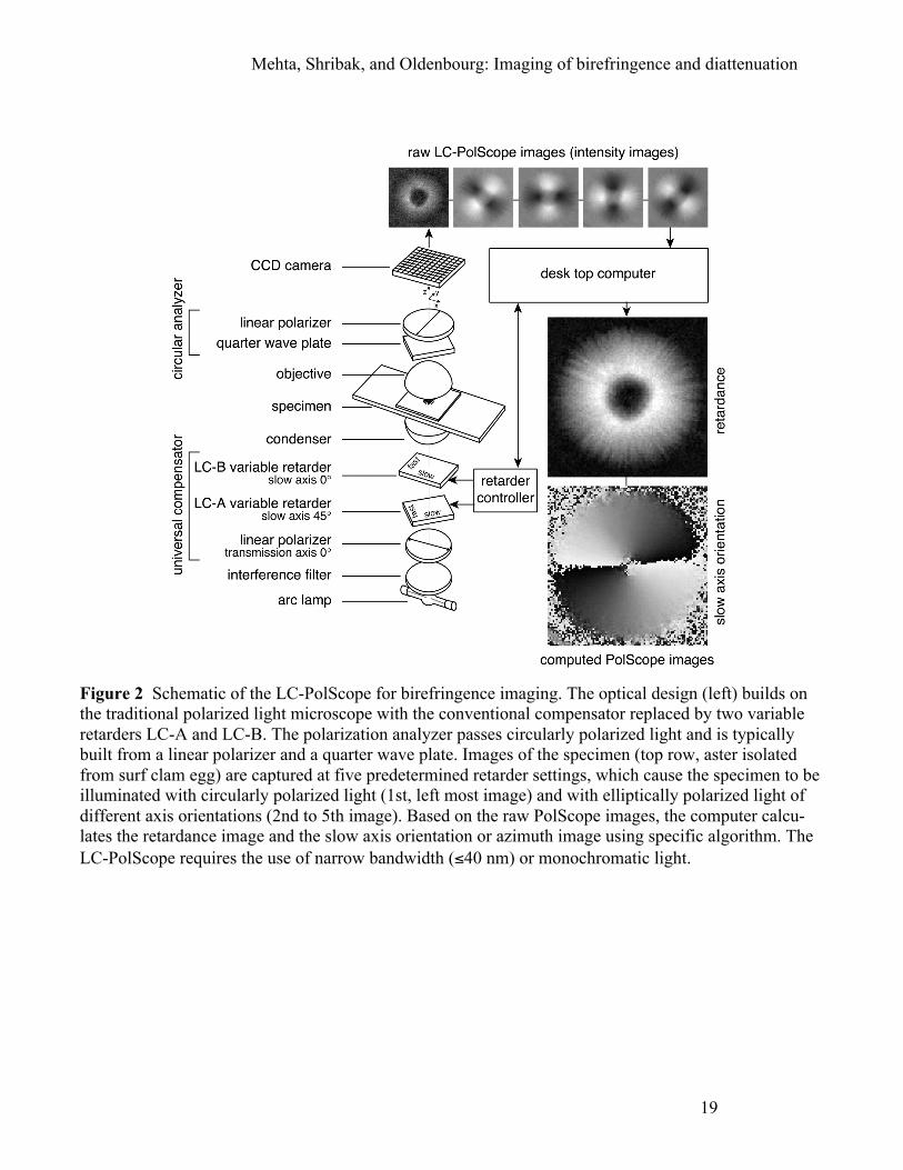
2.1. Birefringence LC-PolScope The optical design of the Birefringence LC-PolScope builds on the traditional polarizing microscope, introducing two essential modifications: the specimen is illuminated with nearly circularly polarized light and the traditional compensator is replaced by a liquid crystal universal compensator. In the sche-matic of Fig. 2, the universal compensator is located between the condenser lens and the light source. The universal compensator is built from two variable retarders and a linear polarizer. The variable re-tarders are implemented as electro-optical devices made from two liquid crystal plates. Each liquid crys-tal plate has a uniform retardance that depends on the voltage applied to the device. An electronic con-troller that is connected to a computer supplies the voltages. The polarization analyzer for circularly po-larized light, placed behind the objective lens, completes the polarization optical train. A CCD or other camera, whose response is linear in the light intensity, records the specimen image that is projected by the objective lens, and specimen images are downloaded to the computer. Specialized software synchro-


4

nizes the image acquisition process with the liquid crystal settings and implements image processing al-gorithms. The algorithms compute images that represent the retardance and slow axis orientation in each resolved image point. A word on units: Retardance can be expressed as a phase angle (in degrees or radians) or as a distance (in nanometer or fraction of wavelength) between two coherent wave fronts. We use the distance be-tween the two wavefronts that are associated with light polarized parallel to the slow and fast axes in the birefringent material. The angle of the slow axis, also called orientation or azimuth, is measured with respect to a laboratory frame of reference, which has its x-axis oriented parallel to the horizontal direc-tion in images. The unique angles of a slow and fast axis range between 0° and 180°, with 190°, for ex-ample, equivalent to 10°.

Next, we summarize the algorithms used for acquiring and processing raw intensity images captured by the camera of the Birefringence LC-PolScope. These are algorithms for measuring parameters of linear birefringence in the absence of circular birefringence and diattenuation.

2.1.1. Algorithms for linear birefringence The light intensity I arriving at the camera sensor depends on several variables, including the specimen retardance (ret) and slow axis orientation (azim), the retardance of LC-A (retLC-A) and LC-B (retLC-B), the maximum amount of light Imax transmitted through the setup, and the minimum amount of light Imin transmitted when the universal compensator is adjusted for extinction:

.

represents the polarization optical train for and . The complete expression for can be found using the Jones Calculus. A detailed discussion of the complete expression and its solutions for the specimen retardance and slow axis orientation is avail-able in (Shribak and Oldenbourg 2003). Here we briefly present the main results. The solutions for specimen retardance and slow axis orientation can be found, based on intensities I0, I1, I2, I3, I4 representing 5 camera images. Each camera image of the specimen is recorded with a specific setting of the liquid crystal retarders of the universal compensator. The first setting generates right circu-larly polarized light, while the next four settings generate elliptically polarized light of equal ellipticity but with orientations of the principal axes that are rotated in steps of 45°. The five settings for retLC-A and retLC-B are best expressed by the differential retardance ∆ by which they deviate from the setting that generates circularly polarized light. For example, circularly polarized light is generated with

and , where is the wavelength of the light. Adding a “swing” value ∆ to one of the retarders, e.g. retLC−A = 0.25λ +Δ , generates elliptical polarization. Light of equal ellipticity but axis orientations that are rotated by 45° are generated by adding or subtracting ∆ from

and in turn. The following expressions represent image intensities record-ed using the five settings. To reduce the complexity of the written expressions we drop all variables ex-cept for ∆, such that for retLC-A = 0.25λ +Δ and retLC-B = 0.5λ , becomes

:

; ; ; ; .

I(ret,azim, retLC-A, retLC-B) = Imax i(ret,azim, retLC-A, retLC-B)+ Imin

i(ret,azim, retLC-A, retLC-B) Imax =1 Imin = 0i(ret,azim, retLC-A, retLC-B)

retLC-A = 0.25λ retLC-B = 0.5λ λ

retLC-A = 0.25λ retLC-B = 0.5λ

I(ret,azim, retLC-A, retLC-B)I(Δ, 0)

I0 = I(0, 0) I1 = I(Δ, 0) I2 = I(0,Δ) I3 = I(0,−Δ) I4 = I(−Δ, 0)


5

As the first setting generates circularly polarized light and leads to extinction after the light has passed through the polarization analyzer, it is called the extinction setting. The others are called elliptical set-tings. Using image arithmetic, first intermediate terms a and b are formed

a = 2(I4 − I1)I1 + I2 + I3 + I4 − 4I0

, b = 2(I3 − I2 )I1 + I2 + I3 + I4 − 4I0

,

which are then used to calculate the specimen retardance ret and azimuth orientation azim:

ret = λ360°

arctan a2 + b2 tan(180°Δλ)

"

#$

%

&' , if I1 + I2 + I3 + I4 − 4I0 ≥ 0 ,

ret = λ360°

180°− arctan a2 + b2 tan(180°Δλ)

#

$%

&

'(

#

$%

&

'( , if I1 + I2 + I3 + I4 − 4I0 < 0 ,

azim = 1

2 arctan(b,a) ,

in which arctan(b, a) represents the arctan ab!

"#$

%&with the signs of a and b considered independently to as-

sign the correct quadrant for the angle.

It is interesting to note that both formulas for ret and azim represent ratios of differences between the raw image intensities I0, I1, I2, I3, I4. Hence, the computed values of ret and azim are independent of the minimum intensity Imin measured at extinction and of the maximum intensity Imax that characterizes the throughput of the system and can vary due to shading or vignetting in the optical path.

To correct for spurious anisotropy that is contributed by optical components such as lenses, mirrors, and the liquid crystal devices, a stack of 5 images is acquired from a clear specimen area that has no bire-fringence. As the lenses and other optical components are still present in the optical path, the back-ground stack records their anisotropies and can be used to remove their effect on the sample images. To do so, we first calculate background values for a and b:

, , , , ;

abg =2(Ibg4 − Ibg1)

Ibg1 + Ibg2 + Ibg3 + Ibg4 − 4Ibg0, bbg =

2(Ibg3 − Ibg2 )Ibg1 + Ibg2 + Ibg3 + Ibg4 − 4Ibg0

.

and are then subtracted from the specimen a and b: and ; and and are used in the formulas for specimen retardance and azimuth, instead of and . This back-ground correction is highly effective and produces correct results for specimen retardance values that are smaller than about 30 nm. For specimen retardance values higher than about 80 nm, the background cor-rection introduces systematic errors in the corrected values (Shribak and Oldenbourg 2003).

2.1.2. Example Fig. 3 shows retardance images recorded with the LC-PolScope, illustrating the clarity, resolution and analytic potential for examining the birefringent fine structure in living cells. It is also testimony to the opportunities still awaiting for polarized light imaging to reveal the architectural dynamics in living

Ibg0 = Ibg(0, 0) Ibg1 = Ibg(Δ, 0) Ibg2 = Ibg(0,Δ) Ibg3 = Ibg(0,−Δ) Ibg4 = Ibg(−Δ, 0)

abg bbg acorr = a− abg bcorr = b− bbg acorrbcorr a b


6

cells, as the structural origins of the birefringence of many of the organelles visible in Fig. 3, such as mitochondria and lipid droplets, remain mysterious.

The commercial LC-PolScope technique, developed and marketed by CRi Inc. (now part of Perki-nElmer), is available as an accessory to microscope stands of all major microscope manufacturers. It usually includes the universal compensator, circular polarizer, a camera with control electronics and a computer with software for image acquisition and processing. Three slightly differing versions are avail-able, optimized for research in the life sciences (Abrio LS), industrial metrology (Abrio IM), and for in vitro fertilization and related laboratory techniques (Oosight).

When equipped for birefringence imaging, the LC-PolScope is also sensitive to diattenuation or dichro-ism, i.e. in the retardance image dichroic structures such as aligned pigments will be visible as aniso-tropic features that induce a differential phase shift (retardance) in the transmitted light. However, in the case of absorbing structures, the apparent retardance assigned by the birefringence algorithm has no di-rect physical meaning. Later, in the section on the “Relationship between dichroism and birefringence measurements” we will comment on this observation further.

In the next section we will describe a modification to the LC-PolScope that converts the instrument from measuring birefringence in the absence of diattenuation, to measuring only diattenuation, largely inde-pendent of differential phase shift due to birefringence.

2.2. Diattenuation LC-PolScope For measuring diattenuation instead of birefringence, one only needs to remove the polarization analyzer from the optical path. Fig. 4 shows a schematic of the Diattenuation LC-PolScope and a graph that illus-trates the intensities measured on the camera sensor when illuminating a diattenuating specimen with linearly polarized light. The differential transmission, or linear diattenuation, of the specimen modulates the measured intensities as the angle of the linear polarization is rotated. The intensity shows a sinusoi-dal variation that has a well-established dependency on the angle of polarization, described as the gener-alized law of Malus (Azzam and Bashara 1973). Based on this functional dependency, it is sufficient to measure the intensity at a small number of predetermined polarization settings, as indicated in the graph. We are using four intensities to calculate parameters such as maximum and minimum transmittance, and the polarization orientation for maximum transmittance, as discussed in the section on algorithms. To establish the transmittance of a specimen, one needs to know the incoming light intensity. Therefore, in addition to recording 4 images with the specimen in the field of view, a stack of background images must be recorded, after removing the specimen from view. In most cases, removal of the specimen is achieved by simply sliding the specimen sideways on the stage to bring a clear area into view. The need for a clear area next to the specimen of interest should be kept in mind when preparing the specimen. The recording of the background stack will also assist in removing instrument bias in the measurement of specimen diattenuation, as will be shown later.

The setup for measuring diattenuation is insensitive to birefringence, which means that the measured intensities do not depend on a differential phase shift that is likely to occur when the light passes through the sample. This feature is a direct consequence of the lack of a polarization analyzer in the imaging path. By way of explanation, any differential phase shift induced by the specimen does not affect the intensity of the light, but can affect its polarization. As the imaging path lacks a polarization analyzer, a change in polarization in the imaging light remains undetected by the setup.

To preserve the insensitivity to birefringence, it is important to avoid any optical components that may be diattenuating themselves, such as a mirror, prism, or beam splitter, in the optical path. If such compo-


7

nents are placed downstream to the universal compensator in the light path, they lead to an instrumental bias that affects the measurement of sample diattenuation. While it is sometimes impossible to avoid components that introduce instrument bias, it is possible to measure the bias by taking recourse to the background stack introduced above. Based on the background stack, the sample images are corrected for the instrument bias, as described in the next section on algorithms. However, as always, it is best to min-imize the instrument bias by choosing the right hardware und start with the cleanest raw images possi-ble. Next we are discussing algorithms for measuring linear diattenuation and give an example of the meas-ured diattenuation of a Siemens star pattern etched into a thin aluminum film. This is followed by a brief summary of measuring circular diattenuation using the same setup.

2.2.1. Algorithm for linear diattenuation In the following, we call linear diattenuation just diattenuation, while we will always put circular in front of diattenuation when we mean circular diattenuation.

For measuring the differential transmittance of diattenuating materials, we use the setup shown in Fig. 4 to record images at predetermined polarization settings. As mentioned earlier, the universal compensator made of a linear polarizer followed by liquid crystal devices LC-A and LC-B is used as a universal po-larizer that can generate any polarization state. For example, linearly polarized light with polarization orientation φ is generated using retLC-B=0.25 λ and retLC-A=λ•φ/180º. Let us consider the intensity of light that has passed through first the universal polarizer, followed by a uniformly diattenuating specimen, and is then projected onto the camera. As we change the orientation of the linear polarization from 0° (horizontal), to 90° (vertical), to 180° (horizontal again), the recorded intensity varies according to the following expression (generalized law of Malus):

I(φ) = 12 Imax + Imin + Imax − Imin( )cos 2(φ − azimuth)( )( ) = 1

2 Ii Tmax +Tmin + Tmax −Tmin( )cos 2(φ − azimuth)( )( ) ,

is the initial intensity measured without diattenuating specimen, Imax = Tmax ⋅ Ii is maximum intensity measured with diattenuating specimen, Tmax is its maximum trans-mittance, Imin = Tmin ⋅ Ii is minimum intensity measured with diattenuating specimen, Tmin is its minimum transmit-tance,

is the polarization orientation that results in maximum transmittance.

To comprehensively describe the characteristics of the specimen’s transmittance, we determine the , its mean transmittance Tmean , and its diattenuation (see for example (Chipman 2010)):

Tmean = 12 Tmax +Tmin( ) , diattenuation = Tmax −Tmin

Tmax +Tmin

To determine these characteristics, we measure the intensity for four linear polarization states whose orientations are rotated by 45° to each other in a laboratory frame of reference:

, , ,

φI(φ)

Ii

azimuth

azimuth

I0 = I(0°) I45 = I(45°) I90 = I(90°) I135 = I(135°)


8

By measuring intensities , , , and entering them together with the corresponding polariza-tion orientations into the expression for , we have 4 equations that can be solved for the unknowns

, Tmean , and diattenuation. We first form intermediate results a, b, and c:

, , ,

and then express the unknowns as a function of those intermediate results:

azim =

arctan(b,a)2

,

diattenuation = Imax − Imin

Imax + Imin=Tmax −TminTmax +Tmin

=2 a2 + b2

c, values 0 … 1.

In addition to diattenuation, the differential transmission may also be expressed in terms of the ratio of Imax to Imin :

ratio = Imax

Imin=TmaxTmin

=1+ diattenuation1− diattenuation

, values 1 … infinity

To calculate the mean transmittance, we make use of the background stack of images and recognize Ii as the mean background intensity:

, hence

Tmean =

I0 + I45 + I90 + I135Ibg0 + Ibg45 + Ibg90 + Ibg135

.

To account for spurious differential attenuation caused by microscope optics, including lenses, mirrors, filters, and the liquid crystal devices, the background stack is also used to correct the sample image stack. To that end, each sample intensity is divided by the corresponding background transmittance,

such as I0 is divided by Tbg0 =Ibg0Ii

, hence:

, , , and

The corrected values Icorr0 through Icorr135 are then used in the expressions for the intermediate results a, b, and c.

As mentioned earlier, all expressions are implemented as image arithmetic operations and are applied to all pixels simultaneously, resulting in azimuth and diattenuation images that represent quantitative maps of differential transmittance, polarization orientation for maximum transmittance, and mean transmit-tance, all measured at the resolution of the microscope optics.

An easy way to recognize the efficacy of correcting the instrumental bias is to record a background stack, followed by a sample stack, both stacks imaging the same clear area. Processing the sample stack without background correction is likely to result in low diattenuation varying slowly across the field of

I0 I45 I90 I135I(φ)

azimuth

a = I0 − I90 b = I45 − I135 c = I0 + I45 + I90 + I135

Ii =Ibg0 + Ibg45 + Ibg90 + Ibg135

4

Icorr0 = I0IiIbg0

Icorr45 = I45IiIbg45

Icorr90 = I90IiIbg90

Icorr135 = I135Ii

Ibg135


9

view. The finite diattenuation in this case is caused by spurious dichroism in components of the micro-scope optical path. The changes in intensity incurred by spurious polarization dependent transmission are carried through the optical system, are projected into the image plane, and are measured as variations in the background diattenuation. However, the data recorded in the background stack record the varia-tions and can be used to remove their effect on the sample data. Hence, a sample stack of a clear area that is corrected in the above manner and then processed, will show minimal and uniform diattenuation across the image plane. Usually the minimal diattenuation is not zero, but varies randomly from pixel to pixel and is caused by the noise (typically shot noise) in the collected image data. These random varia-tions in diattenuation due to shot noise set a lower limit on the sample diattenuation that can be reliably measured.

When inspecting the azimuth data that result from processing the sample stack without background cor-rection, one typically recognizes azimuth values that vary slowly across the image. Processing the same sample data with background correction results in an azimuth image that is uniform across the image and azimuth data randomly vary from pixel to pixel between 0° and 180°. This random variation is again caused by the shot noise in the raw image data. Next, we illustrate the sensitivity and resolution afforded by the Diattenuation LC-PolScope, demon-strated by a nanofabricated star pattern etched into a thin metal film.

2.2.2. Example Fig. 5 shows the mean transmittance, diattenuation, and apparent retardance of a Siemens star etched by electron lithography into a thin metal film (Oldenbourg et al. 1996). The radial spoke pattern of 36 wedge pairs represents a grating of varying orientation and with a periodicity that increases with increas-ing distance from the center of the pattern. The image was projected by a 40x Fluor (Nikon) oil immer-sion objective with a diaphragm in the back focal plane to set the objective’s numerical aperture to 0.5. The average transmittance near the central part of Fig. 5 B displays the expected resolution according to the wavelength = 630 nm and the NA of 0.5 that was set for both, objective and condenser lens. In addition, the anisotropy of the pattern, which is revealed in panels C and D by the polarization depend-ent phase shift (apparent retardance) and transmittance (diattenuation) shows interesting features, which we describe here qualitatively, but leave a quantitative evaluation to a future publication.

The modulation of the intensity approaches zero for a radius of 3.9 µm, which corresponds to a periodic-ity of , close to the expected value of the resolution limit for the NA and wave-length used ( ). The modulation increases for larger radii, while for smaller radii the modulation remains flat.

At an even smaller radius of 1.8 µm, the transmittance increases almost twofold to remain high until the finer and finer grating ends at the central disk (radius 0.6 µm). The grating at a radius of 1.8 µm has a periodicity of 0.315 µm, which is half the wavelength of the light used. Panel C in Fig. 5 shows the retardance near the center and panel D shows its differential transmittance for linear polarization, measured with the diattenuation mode of the LC-PolScope. For radii larger than 3.9 µm, where wedge edges are resolved, low diattenuation is observed near the wedge edges. However, in the unresolved central part of the pattern, one can recognize two bright, highly diattenuating rings separated by a dark ring. The outer ring is the most diattenuating feature of the pattern, but transmits low light. The inner ring transmits more light but is less diattenuating.

λ

2 ⋅3.9 ⋅π / 36 = 0.68 µmλ / (2 NA) = 0.63µm


10

The periodicity of the pattern that is responsible for the innermost ring of anisotropy is smaller than half the wavelength of light. Grid patterns of those dimensions are called wire grid polarizers and their action is well understood (Bennett 2010). Wire grid polarizers reflect the light whose electric field is polarized parallel to the linear wires. Hence, maximum transmittance through the wire grid is observed for the po-larization that is perpendicular to the wire orientation, which corresponds to the azimuthal alignment of the lines that indicate the orientation of high transmittance in the innermost ring of panel D in Fig. 5.

The origin of the high diattenuation and phase shift observed for periodicities between and of the wavelength must be related to a resonance in the interaction between the wire grid pattern and the light field of similar periodicities. We are leaving a quantitative evaluation of those phenomena to a fu-ture publication, but point out that the retardance measurement using the Birefringence LC-PolScope includes both effects, differential transmittance and differential phase shift. Hence, the apparent retard-ance cannot be interpreted as a phase shift alone, but its interpretation has to also account for the diat-tenuation, which is measured by the Diattenuation LC-PolScope without interference from differential phase shifts, as discussed in section 3.

2.2.3. Algorithm for circular diattenuation For measuring circular diattenuation, we can use the same setup as shown in Fig. 4 and acquire images of the specimen when it is trans-illuminated with left and right circularly polarized light, instead of line-arly polarized light. The two circular polarizations can be generated using retLC-A = 0.25λ and retLC-A = 0.75λ, keeping retLC-B constant at 0.5λ. Specimen components that exhibit circular diattenuation will have a non-zero differential transmittance Tleft −Tright , with Tleft and Tright the transmittance for left and right circularly polarized light, respectively. Circular diattenuation has no azimuth orientation associated with it. Similar to the transmittance for linearly polarized light, we define the material parameters for circularly polarized light as mean circular transmittance CTmean and circular_diattenuation:

CTmean = 12 Tleft +Tright( ) , and

circular _ diattenuation =Tleft −TrightTleft +Tright

,

with I left = Tleft ⋅ Ii and Iright = Tright ⋅ Ii and Ii the incoming intensity. Again, we find Ii using the intensi-

ties measured in a clear area of the specimen, Ii = 12 Ibg left + Ibg right( ) , and use Ibg left and Ibg right to correct

for possible instrument bias:

Icorr left = I leftIi

Ibg left

, Icorr right = IrightIi

Ibg right

,

CTmean =Icorr left + Icorr right

2 Ii, and

circular diattenuation =Icorr left − Icorr right

Icorr left + Icorr right

.

λ / 2 λ


11

3. Relationship between diattenuation and birefringence measurements

3.1. Birefringence and orientation of slow axis Birefringence occurs when there is a molecular order, when the average molecular orientation is non-random, as in crystals or in aligned polymeric materials. For a given propagation direction of light, mo-lecular order usually gives the material two orthogonal optical axes, with the index of refraction for light polarized along one axis being different from the other axis. The difference between the two indices of refraction is called birefringence, and is an intrinsic property of the material: birefringence = ,

where and are the refractive indices for light polarized parallel and perpendicular to the two opti-cal axes. We note for the above expression, birefringence refers to the cross section between the refrac-tive index ellipsoid of the material and the plane whose normal is the propagation direction of the light. This is also called the birefringence of the section, in contrast to the maximum or substance birefrin-gence observed for a uniaxial material when the optic axis is located in the plane of observation (Hartshorne and Stuart 1960).

Light polarized parallel to one axis travels at a different speed through the sample than light polarized perpendicular to that axis. As a result, the two light components, which were in phase when they entered the sample, are retarded at a different rate and exit the sample out of phase. Using the polarizing micro-scope, one can measure this differential retardation, also called retardance, and thereby quantify the magnitude and orientation of molecular order in the specimen. Retardance is an extrinsic property of the material and a product of the birefringence and the path length l through the material: retardance = .

Retardance refers to the differential phase shift between orthogonal polarization components. However, if differential transmittance cannot be neglected in the specimen, the Birefringence LC-PolScope measures a retardance that not only reports the differential phase shift but is also affected by the differ-ential transmittance in the material (see section “Measuring differential transmittance as retardance”).

Birefringence also has an orientation associated with it. The orientation refers to the specimen’s optical axes of which one is called the fast axis and the other the slow axis. Light polarized parallel to the slow axis experiences a high refractive index and travels slower than light polarized parallel to the fast axis. In materials that are built from aligned filamentous molecules, the slow axis is typically parallel to the average orientation of the filaments. Birefringence orientation always correlates with molecular orienta-tion, which usually changes from point to point in the specimen.

Like retardance, the orientation of the slow axis measured by the Birefringence LC-PolScope is also af-fected by diattenuation present in the material, as discussed later.

For a more comprehensive discussion of birefringence of optically anisotropic materials, see (Hartshorne and Stuart 1960; Hecht 2002; Shurcliff 1962).

3.2. Linear diattenuation and orientation of maximum transmittance Linear diattenuation is a material property that can occur in absorbing materials in which the light ab-sorbing molecules or fine structure are arranged with a preferred orientation. Diattenuation refers to the difference in transmittance for light polarized at specific angles to the principal axis of alignment.

€

Δn = n|| − n⊥

€

n||

€

n⊥

€

R = Δn ⋅ l


12

Diattenuation and dichroism describe similar material properties and their relationship can be confusing. Additional confusion arises from the fact that dichroism has two related but distinct meanings in optics. A dichroic material is either one which causes visible light to be split up into distinct beams of different wavelengths, or one in which light rays having different polarizations are absorbed at different rates. The latter meaning describes a similar material property as diattenuation. Dichroism describes the prop-erty in terms of the material's absorption and diattenuation in terms of its transmittance. As we are con-cerned with light that is transmitted through the sample, and not the part that is absorbed, we refer to the instrument as Diattenuation LC-PolScope.

For a given propagation direction of light, the molecular alignment creates two principal axes in the ma-terial. When light is polarized parallel to one axis, the material has maximum transmittance Tmax , and when it is polarized parallel to the other axis, its transmittance Tmin is a minimum. The two axes are nec-essarily orthogonal to each other. When light of intensity is polarized at an arbitrary angle and en-

ters the material, it is split into two components; one ( ) polarized parallel to the direction of

high transmittance and one ( ) is polarized perpendicular to it. When the two components leave the material boundaries, they recombine and are detected as light that was transmitted with a transmit-tance T (θ ) that depends on the polarization angle θ of the incoming light. The total detected intensity is simply the sum of the intensity of both polarized components in the absence of a polarizing element be-tween the material and the detector. Thus,

Ii T (θ ) = Ii Tmax cos2θ + Ii Tmin sin

2θ = 12 Ii Tmax +Tmin + Tmax −Tmin( )cos2θ( )

The above expression is identical to the earlier expression that was identified as a generalization of the law of Malus, with the azimuth variable set to zero. When azimuth is zero, the principal axes of the ma-terial coincide with the laboratory frame of reference.

With the Diattenuation LC-PolScope we can measure the mean transmittance Tmean = 12 Tmax +Tmin( ) , the

differential transmittance, and the angle of maximum transmittance in the form of high-resolution imag-es of the sample, documenting even subtle variations that reflect the molecular order changing from point to point in the sample. Importantly, diattenuation measurements are largely unaffected by differen-tial phase shifts that are induced by concomitant birefringence in the sample. However, as mentioned earlier, the Birefringence LC-PolScope is sensitive to both, birefringence and diattenuation. Next, we briefly discuss this somewhat confusing distinction between the two modes of measurement.

3.3. Measuring diattenuation as retardance As mentioned earlier, the Birefringence LC-PolScope is sensitive to both, birefringence and diattenua-tion. The polarization analyzer in the light path of the Birefringence LC-PolScope makes the instrument sensitive to changes in polarization, regardless if they are incurred by birefringence or diattenuation in the specimen. By way of explanation, let’s consider a diattenuating structure like the wire grid polarizer formed by the unresolved pattern near the center of the Siemens star in Fig. 5. When light of arbitrary polarization angle enters the grid, it is split into two components, one polarized parallel and the other perpendicular to the grid lines, and each is attenuated at a different rate. When the components leave the grid, their superposition will generally lead to a polarization that is different from the light entering the grid, because the amplitudes of the two components are different from before the grid. As a change in polarization is the primary signal that is analyzed by the birefringence measurement setup of Fig. 2, the grid will cause an apparent retardance solely based on the fact that the two polarization components

Ii θ

Ii cos2(θ )

Ii sin2(θ )


13

were subject to differential transmittance. However, if referred to as a differential phase shift, the diat-tenuation-induced retardance has no physical meaning and has to be considered a measurement artifact. In addition, diattenuation-induced retardance has an apparent slow axis orientation that is rotated by 45° with respect to the axis of maximum transmittance. (One can prove this point using the Jones Calculus, for example.) The apparent retardance and slow axis orientation is added to any real differential phase shift that is likely to occur for a diattenuating material. The superposition of apparent and real phase shifts that are measured together in the Birefringence LC-PolScope lead to the skewed angle of slow ax-is orientation observed in the retardance image of the central part of the Siemens star in Fig. 5C.

This latter feature can actually help in identifying a retardance measurement that is “contaminated” by differential transmittance. Let us look again at the slow axis orientation in Fig. 5C. It has an angle that is neither parallel nor perpendicular to the grid lines and is therefore suspect. There is no physical reason for the true differential phase shift to have a symmetry, i.e. orientation of its slow and fast axis, that is different from the symmetry of the grating itself. The twist of the slow axis in Fig. 5C is caused by both, the grid and the measurement apparatus together, and is not a physical property of the grid alone. How-ever, as the measurement of the differential transmittance is unaffected by differential phase shift, we believe the two measurements together can be used to remove the effect of differential transmission on the measured retardance. We leave a more detailed analysis of this statement to a future publication. In the last section, we briefly touch on the fact that diattenuation is always accompanied by differential phase shift, making the feature of insensitivity to phase shift especially valuable in the Diattenuation LC-PolScope.

3.4. Physical relationship between birefringence and diattenuation Diattenuation and birefringence refer to the polarization dependence of the two, more basic phenomena of absorption and refraction, respectively. Both these phenomena are the consequence of light interact-ing with matter and are therefore closely related, to the point that one would not exist without the other (Feynman et al. 1963). We briefly discuss this close relationship, with the intent to develop an intuitive understanding for the reader. The refractive index is an expression of refraction that occurs because of the electric field emitted by electrons that oscillate in a material in response to the incident light. The oscillations of electrons that are forced by the incident field cause secondary radiation that has a fixed phase relationship with the in-coming light. The secondary radiation, when combined coherently with the incident radiation, results in a slowed wave front, which leads to the phenomenon of refraction. The refractive index directly de-scribes the degree of slowdown. The amplitude and phase response of the electron cloud depends on the wavelength (or frequency) of the light – a phenomenon called dispersion. At frequencies near a reso-nance, the secondary radiation can be opposite in phase to the incident radiation, reducing the amplitude of the transmitted radiation significantly and leading to the phenomenon of absorption or reduced trans-mittance. Birefringence and diattenuation, expressing the polarization dependence of refraction and transmittance, occur when the oscillating electron clouds have restoring forces that depend on the mutu-al angle between the polarization of the incident light and the orientation of molecular and/or fine struc-tural order of the material.

Most biological materials, like carbohydrates, proteins and nucleic acids, absorb in the ultraviolet at fre-quencies that are higher than the visible spectrum of light. The material refractive index in the visible regime is an expression of the strength and anisotropy of the resonances that occur in the ultraviolet. Usually, the refractive index and birefringence of those materials vary little over a large frequency range in which no absorption occurs.


14

Other biological materials, like pigments and light absorbing proteins in the retina, absorb in the visible spectrum, resulting in absorption spectra that are quite specific to the pigments involved. Therefore, spectrally resolved absorption and diattenuation measurements have the potential to provide specificity to molecular order and molecular composition.

4. Further readings The classic books on polarizing microscopy were published several decades ago, when optical phase microscopy was in its heydays (Hartshorne and Stuart 1960; Hartshorne and Stuart 1964). Several dec-ades before Hartshorne, W. J. Schmidt published 2 celebrated monographs that to this day report the most comprehensive surveys of biological specimens observed under polarized light (Schmidt 1924; Schmidt 1937). Inspired by Schmidt’s observations, Shinya Inoué significantly improved the sensitivity of the instrument and made seminal contributions to our understanding of the architectural dynamics in-side living cells (Inoue et al. 1975; Inoué and Hyde 1957; Inoue and Sato 1967). For many lucid discus-sions of polarized light microscopy and its application to biology, we refer the reader to the many arti-cles and books by Inoué, including his recently published Collected Works (Inoue 2002; Inoué 1986; Inoué 2003; Inoué 2008; Inoue and Oldenbourg 1998). Tinoco and collaborators reviewed the imaging of dichroism and diattenuation in biological materials (Tinoco et al. 1987). Jin et al. applied the rotating-polarizer method to studying the linear birefringence and diattenuation in cerebral amyloid pathologies (Jin et al. 2003). The following articles include the LC-PolScope in their discussion of various aspects of polarizing microscopy (Oldenbourg 1999; Oldenbourg 2005; Oldenbourg 2007; Oldenbourg and Shribak 2010; Shribak and Oldenbourg 2003). A glossary of polarization optical terms, such as retard-ance and slow axis, is contained in (Oldenbourg 2013)

5. Conclusion Polarized light microscopy allows one to nondestructively follow the dynamic organization of living cells and tissues at the microscopic as well as submicroscopic levels. Imaging with polarized light re-veals information about the organization of the endogenous molecules that built the complex and highly dynamic architecture of cells and tissues. We have shown that the LC-PolScope can be used for imaging birefringence, linear and circular diattenuation, and is thus a versatile tool to reveal information about structural parameters, such as the alignment of molecular bonds and their transition moments, and of the chirality of molecules.

We believe, with current instrumentation we have only scratched the surface of the potential of polarized light microscopy and we look forward to more advances that will emerge with combining hardware and software components with new insights into the interaction of polarized light with the building blocks of man-made and natural materials.

6. Acknowledgments The authors gratefully acknowledge many years of illuminating discussions on polarized light microsco-py with Shinya Inoué of the MBL. Grant Harris and Amitabh Verma implemented image acquisition and processing software.

This work was supported by a fellowship of the Human Frontiers Science Program awarded to SM and a grant from the National Institute of Biomedical Imaging and Bioengineering (grant Nr. R01EB002045) awarded to RO. MS acknowledges support from the National Institute of General Medical Sciences/NIH (grant R01-GM101701).


15

7. References Allen RD, Brault J, Moore RD. 1963. A new method of polarization microscopic analysis I. Scanning

with a birefringence detection system. J Cell Biol 18:223-235. Azzam RMA, Bashara NM. 1973. Polarization-dependent intensity transmittance of optical systems.

Applied Physics 1(4):203-212. Bennett JM. 2010. Polarizers. In: Michael Bass CD, Jay M. Enoch, Vasudevan Lakshminarayanan,

Guifang Li, Carolyn Macdonald, Virendra N. Mahajan, Eric Van Stryland, editor. Handbook of Optics. 3rd ed. New York: McGraw-Hill, Inc. p 13.11 - 13.65.

Byrne JA, Pedersen DA, Clepper LL, Nelson M, Sanger WG, Gokhale S, Wolf DP, Mitalipov SM. 2007. Producing primate embryonic stem cells by somatic cell nuclear transfer. Nature 450(7169):497-502.

Chipman RA. 2010. Polarimetry. In: Michael Bass CD, Jay M. Enoch, Vasudevan Lakshminarayanan, Guifang Li, Carolyn Macdonald, Virendra N. Mahajan, Eric Van Stryland, editor. Handbook of Optics. 3rd ed. New York: McGraw-Hill, Inc. p 15.11 - 15.46.

Feynman RP, Leighton RB, Sands M. 1963. The origin of the refractive index. The Feynman Lectures on Physics. Reading, Massachusetts: Addison-Wesley Publishing Co.

Glazer AM, Lewis JG, Kaminsky W. 1996. An automatic optical imaging system for birefringent media. Proc R Soc London, A 452:2751-2765.

Hartshorne NH, Stuart A. 1960. Crystals and the Polarising Microscope: A Handbook for Chemists and Others. London: Arnold.

Hartshorne NH, Stuart A. 1964. Practical Optical Crystallography. New York, NY: American Elsevier Publishing Co., Inc.

Hecht E. 2002. Optics. San Francisco, CA: Pearson/Addison-Wesley. Inoue S. 2002. Polarization microscopy. Curr Protoc Cell Biol Chapter 4:Unit 4 9. Inoué S. 1986. Video Microscopy. New York: Plenum Press. Inoué S. 2003. Exploring living cells and molecular dynamics with polarized light microscopy. In:

Török P, Kao FJ, editors. Optical Imaging and Microscopy. 2nd ed. Berlin, Heidelberg, New York: Springer-Verlag. p 3-20.

Inoué S. 2008. Collected Works of Shinya Inoué: microscopes, living cells, and dynamic molecules. Singapore: World Scientific.

Inoue S, Fuseler J, Salmon ED, Ellis GW. 1975. Functional organization of mitotic microtubules. Physical chemistry of the in vivo equilibrium system. Biophys J 15(7):725-744.

Inoué S, Hyde WL. 1957. Studies on depolarization of light at microscope lens surfaces II. The simultaneous realization of high resolution and high sensitivity with the polarizing microscope. J Biophys Biochem Cytol 3(6):831-838.

Inoue S, Oldenbourg R. 1998. Microtubule dynamics in mitotic spindle displayed by polarized light microscopy. Mol Biol Cell 9(7):1603-1607.

Inoue S, Sato H. 1967. Cell motility by labile association of molecules. The nature of mitotic spindle fibers and their role in chromosome movement. J Gen Physiol 50(6):Suppl:259-292.

Jin LW, Claborn KA, Kurimoto M, Geday MA, Maezawa I, Sohraby F, Estrada M, Kaminsky W, Kahr B. 2003. Imaging linear birefringence and dichroism in cerebral amyloid pathologies. Proc Natl Acad Sci U S A 100(26):15294-15298.

Kaminsky W, Gunn E, Sours R, Kahr B. 2007. Simultaneous false-colour imaging of birefringence, extinction and transmittance at camera speed. J Microsc 228(Pt 2):153-164.


16

Keefe D, Liu L, Wang W, Silva C. 2003. Imaging meiotic spindles by polarization light microscopy: principles and applications to IVF. Reprod Biomed Online 7(1):24-29.

Kuhn JR, Wu Z, Poenie M. 2001. Modulated polarization microscopy: a promising new approach to visualizing cytoskeletal dynamics in living cells. Biophys J 80(2):972-985.

Laude-Boulesteix B, De Martino A, Drevillon B, Schwartz L. 2004. Mueller polarimetric imaging system with liquid crystals. Appl Opt 43(14):2824-2832.

Le Floch A, Ropars G, Enoch J, Lakshminarayanan V. 2010. The polarization sense in human vision. Vision Res 50(20):2048-2054.

Liu L, Oldenbourg R, Trimarchi JR, Keefe DL. 2000. A reliable, noninvasive technique for spindle imaging and enucleation of mammalian oocytes. Nat Biotechnol 18(2):223-225.

Mathger LM, Shashar N, Hanlon RT. 2009. Do cephalopods communicate using polarized light reflections from their skin? J Exp Biol 212(Pt 14):2133-2140.

Oldenbourg R. 1999. Polarized light microscopy of spindles. Methods Cell Biol 61:175-208. Oldenbourg R. 2005. Polarization microscopy with the LC-PolScope. In: Goldman RD, Spector DL,

editors. Live Cell Imaging: A Laboratory Manual. Cold Spring Harbor, NY: Cold Spring Harbor Laboratory Press. p 205-237.

Oldenbourg R. 2007. Analysis of microtubule dynamics by polarized light. Methods Mol Med 137:111-123.

Oldenbourg R. 2013. Polarization Microscopy. In: Shaked NT, Zalevskey Z, Satterwhite L, editors. Biomedical Optical Phase Microscopy and Nanoscopy. Amsterdam: Elsevier.

Oldenbourg R, Inoué S, Tiberio R, Stemmer A, Mei G, Skvarla M. 1996. Standard test targets for high resolution light microscopy. In: Hoch HC, Jelinsky LW, Craighead H, editors. Nanofabrication and Biosystems: Integrating Material Science, Engineering and Biology. Cambridge, England: Cambridge University Press. p 123-138.

Oldenbourg R, Mei G. 1995. New polarized light microscope with precision universal compensator. J Microsc 180:140-147.

Oldenbourg R, Mei G; Marine Biological Laboratory (Woods Hole, MA), assignee. 1996. Polarized Light Microscopy. USA patent 5,521,705.

Oldenbourg R, Shribak M. 2010. Microscopes. In: Michael Bass CD, Jay M. Enoch, Vasudevan Lakshminarayanan, Guifang Li, Carolyn Macdonald, Virendra N. Mahajan, Eric Van Stryland, editor. Handbook of Optics. 3rd ed. New York: McGraw-Hill, Inc. p 28.21 - 28.62.

Reppert SM, Gegear RJ, Merlin C. 2010. Navigational mechanisms of migrating monarch butterflies. Trends Neurosci 33(9):399-406.

Schmidt WJ. 1924. Die Bausteine des Tierkörpers in polarisiertem Lichte. Bonn: Cohen. Schmidt WJ. 1937. Die Doppelbrechung von Karyoplasma, Zytoplasma und Metaplasma. Berlin:

Bornträger. Shribak M. 2011. Complete polarization state generator with one variable retarder and its application for

fast and sensitive measuring of two-dimensional birefringence distribution. J Opt Soc Am A Opt Image Sci Vis 28(3):410-419.

Shribak M, Oldenbourg R. 2003. Techniques for fast and sensitive measurements of two-dimensional birefringence distributions. Appl Opt 42(16):3009-3017.

Shribak M, Oldenbourg R; Marine Biological Laboratory (Woods Hole, MA), assignee. 2007a. Retardance Measurement System and Method. USA patent 7,202,950.

Shribak M, Oldenbourg R; Marine Biological Laboratory (Woods Hole, MA), assignee. 2007b. Retardance Measurement System and Method. USA patent 7,239,388.


17

Shribak M, Oldenbourg R; Marine Biological Laboratory (Woods Hole, MA), assignee. 2008. Retardance Measurement System and Method. USA patent 7,372,567.

Shribak M, Oldenbourg R, Cronin PJ, Hoyt CC, Miller PJ; Marine Biological Laboratory (Woods Hole, MA), assignee. 2006. Instantaneous Polarization Measurment System and Method. USA patent 7,079,247.

Shurcliff WA. 1962. Polarized Light, Production and Use. Cambridge, MA: Harvard University Press. Tinoco I, Jr., Mickols W, Maestre MF, Bustamante C. 1987. Absorption, scattering, and imaging of

biomolecular structures with polarized light. Annu Rev Biophys Biophys Chem 16:319-349.


18

8. Figures

Figure 1 Polarized light images of a primary spermatocyte from the crane fly, Nephrotoma suturalis, taken (A) with the traditional polarized light microscope and (B) with the LC-PolScope. In both images variation of brightness is caused by the birefringence of cell structures, like the meiotic spindle near the center. However, in the traditional polarized light image, brightness is a function of both, the orientation of the spindle with respect to the polarizers and compensators of the instrument, and a function of the magnitude of birefringence. In the LC-PolScope image, brightness is directly proportional to the bire-fringence of the specimen, independent of the orientation of the birefringence axis (slow axis). The LC-PolScope image of the flattened cell reveals with great clarity the birefringence of spindle microtubules extending from the chromosomes to the spindle poles, and of astral microtubules radiating from the cen-trosomes located near the poles. The birefringence of other cell organelles such as elongated mitochon-dria, surrounding the spindle like a mantle, and small spherical lipid droplets, is also evident against the dark background of the cytoplasm. The pole-to-pole distance is approximately 25"m.

A B


19

Figure 2 Schematic of the LC-PolScope for birefringence imaging. The optical design (left) builds on the traditional polarized light microscope with the conventional compensator replaced by two variable retarders LC-A and LC-B. The polarization analyzer passes circularly polarized light and is typically built from a linear polarizer and a quarter wave plate. Images of the specimen (top row, aster isolated from surf clam egg) are captured at five predetermined retarder settings, which cause the specimen to be illuminated with circularly polarized light (1st, left most image) and with elliptically polarized light of different axis orientations (2nd to 5th image). Based on the raw PolScope images, the computer calcu-lates the retardance image and the slow axis orientation or azimuth image using specific algorithm. The LC-PolScope requires the use of narrow bandwidth (≤40 nm) or monochromatic light.


20

Figure 3 Birefringence LC-PolScope images with slow axis lines of the primary spermatocyte shown in Fig. 1. At the top left, the retardance image of the whole cell is dominated by the meiotic spindle extend-ing between two poles and with chromosomes aligned at the metaphase plate. Regions 1, 2 and 3 are shown enlarged with red lines indicating the slow axis direction for each pixel. The underlying retard-ance images were enlarged using bilinear interpolation. Region 1 shows a cross section through the cell membrane in which the slow axis is oriented perpendicular to the plane of the membrane. Region 2 identifies a kinetochore with centromere and attached kinetochore fiber, with slow axes parallel to the microtubule bundles. Region 3 shows on the right a lipid droplet with a highly birefringent shell and slow axes perpendicular to the droplet’s surface. The left side of Region 3 shows parts of mitochondria that surround the meiotic spindle like a mantle of birefringent tubes, with a slow axis parallel to the tube axis. (The cell was prepared and the image recorded by James R. LaFountain, University at Buffalo)

1 23

1

2 3

0 1 retardance [nm]

2


21

Figure 4 Diattenuation measurement scheme. The schematic of the optical setup includes the universal compensator (polarizer, LC-A, LC-B) that is used to create linearly polarized light for illuminating the sample. No polarization analyzer is present in the imaging path. (The reverse is possible too, i.e. using unpolarized light as illumination and analyzing the linear polarization of the imaging light.) The graph on the right shows the expected intensity measured in a region of uniform dichroism with a maximum transmittance for light that is linearly polarized at an azimuth orientation of 146°. The solid line is the expected sinusoidal variation when continuously varying the polarization orientation, with intensities labeled for orientations 0° (horizontal), 45°, 90°, and 135°.

from PC

LC-B LC-A

polarizer

a camera

sample

interference filter

halogen lamp

b to PC


22

Figure 5 LC-PolScope images of a Siemens star etched into a 50 nm thick aluminum film on cover glass using electron lithography. The cover glass with film was mounted on a microscope slide using Permount. A Average transmittance of the star pattern, which consists of 36 wedge pairs and has an out-side diameter of 75 µm. Near the outer edge along the circumference the grating period is 6.5 µm, which decreases continuously towards the smallest period of 0.1 µm near the inner black disk (dia. 1.2 µm). Near the white dashed circle, the period is 0.5 λ, and λ near the solid circle, with λ the wavelength of the illuminating light (630 nm). The square outlines the magnified portion in panels B to D. B to D Central portion of the Siemens star imaged with the LC-PolScope in different imaging modes: B Mean transmit-tance. Gray scale legend between panels A and B indicates mean transmittance and applies to both pan-els. C Apparent retardance of the central pattern with red lines indicating the slow axis orientation. D Diattenuation of the central pattern with red lines indicating the orientation of the maximum transmit-tance. In panels C and D lines are drawn for every 3rd pixel of the original image. Gray scale legend be-tween panels C and D shows retardance scale for left and anisotropy scale for right panel. Scale bar in central part of the Figure applies for images in panels B to D.

Documents

Journal of Optics Special issue on High Resolution Optical Imaging