Embed Size (px)
Citation preview


JOURNAL OF MATERIALS AND ENGINEERING STRUCTURES « JMES » COMITÉ EDITORIAL/EDITORIAL BOARD Editeur en Chef/Editor in Chief
• Dr. Farid ASMA, Université Mouloud Mammeri de Tizi-Ouzou, Algeria Comité Scientifique /Scientific Committee
• Pr. Hakim S. ABDELGADER, Department of Civil Engineering, Tripoli University, Tripoli, Libya • Dr. Sidi Mohammed AISSA MAMOUNE, Centre universitaire d'Ain Temouchent, Algeria • Pr. Abdenour ALLICHE, Université Paris 6, France • Pr. Ouali AMIRI, Université de Nantes, France • Dr. Ahmed BENAMAR, Université du Havre LOMC UMR 6294 CNRS, France • Pr. Laurent BLERON, Ecole Nationale Supérieure d’Arts et Métiers, France • Pr. Mokhtar BOUNAZEF, Université de Sidi Bel Abbès, Algeria • Dr. Mohand CHAOUCHE, Ecole Normale Supérieure de Cachan, France • Pr. Kamel CHAOUI, Université d’Annaba, Algeria • Pr. Hélène DUMONTET, Université Pierre et Marie Curie de Paris 6, France • Pr. Khalil EL-HAMI, University of Hassan 1, Faculty of Khouribga, Morocco • Pr. Abdellatif IMAD, Ecole Polytechnique Universitaire de Lille, France • Dr. Xiaopeng HUANG, Massachusetts Institute of Technology, Cambridge, USA • Pr. Moussa KARAMA, Ecole Nationale d’Ingénieurs de Tarbes, France • Pr. Jamal KHATIB, Faculty of Science and Engineering, University of Wolverhampton, UK • Pr. Abdelhafid KHELIDJ, Université de Nantes, France • Pr. Fekri MEFTAH, Université de Cergy-Pontoise, France • Dr. Taghreed Khaleefa MOHAMMED ALI, Koyauniversity, Iraq • Pr. Kamal MOHAMMEDI, M. Bougara University, Boumerdès MESOnexusteam/LEMI, Algeria • Dr. Marc OUDJENE, Université de Lorraine, France • Pr. Kheir-Eddine RAMDANE, Université des Sciences et de la Technologie d'Oran, Algeria • Dr. Jaroslaw Rybak, Wroclaw University of Technology, Poland • Pr. Khemais SAANOUNI, Université de Technologie de Troyes, France • Dr. Abdussalam SHIBANI, Faculty of Engineering and Computing, Coventry University, UK • Dr. Mohamed SONEBI, Queen's University, Belfast, Northern Ireland, UK • Pr. Abelkader TAHAKOURT, Université A. M. de Béjaia, Algeria • Pr. Redouane ZITOUNE, Université de Toulouse, France
Assistants éditoriaux / Editorial Assistants
- Melle. Djamila MANSOUR - Mr. Said CHEKLAT Email: [email protected] Site : http://revue.ummto.dz/index.php/JMES

JOURNAL OF MATERIALS AND ENGINEERING STRUCTURES 1 (2014) 119–168
Journal of Materials and Engineering Structures Vol. 1, No. 3, December (2014) Table of Contents
Creep investigation of GFRP RC Beams - Part A : Literature review and experimental Study Masmoudi Abdelmonem, Mongi Benouezdou, Mohamed Beldi, André Weber
119
Creep investigation of GFRP RC Beams - Part B: A theoretical framework Masmoudi Abdelmonem, Mongi Benouezdou, Mohamed Beldi, André Weber
127
Buckling Response of Thick Functionally Graded Plates Bouazza Mokhtar, Abedlouahed Tounsi, EL Abbas Adda-Bedia
137
Determination of the performance point of reinforced concrete frames using the nonlinear static method pushover
Abdelouafi El Ghoulbzouri, El Alami Zakaria, Sabrine El Hannoudi
146
Behavior of a gravel-sand material on cyclic way Hocine Bendadouche, Kaddour Khemmoudj, Smail Merabet
155
ISSN 2170-127X
This work is licensed under a Creative Commons Attribution-ShareAlike 4.0 International License. Based on a work at http://revue.ummto.dz.

JOURNAL OF MATERIALS AND ENGINEERING STRUCTURES 1 (2014) 119–126 119
Research Paper
Creep investigation of GFRP RC Beams - Part A: Literature review and experimental Study
Abdelmonem Masmoudi*,a, Mongi Ben Ouezdou b, Mohamed Beldi b, André Weber c a Laboratory of Mechanics, Modeling and Manufacturing, National School of Engineers of Sfax, Tunisia b Civil Engineering Laboratory, National Engineering School of Tunis, B.P 1173, 3038, Tunisia c Research and Development Center, FRP Combar Schöck, Baden-Baden, Germany
A R T I C L E I N F O
Article history :
Received 7 July 2014
Accepted 2 September 214
Keywords:
Concrete, GFRP Bars,
Superposition principle
Return creep reloading,
Viscoelasticity elasticity
A B S T R A C T
GFRP composite bars are excellent alternative to steel bars for reinforcing concrete structures in severe environments. However, studies on creep phenomenon of GFRP reinforced concrete structures are limited. Creep occurs as a result of long term exposure to high levels of stress that are below the yield strength of the material.
This paper (Part A) presents a literature review and the loading history of six experimental beams reinforced with GFRP and steel bars. The results of this study revealed that Beams reinforced with GFRP are less marked with creep phenomenon. This investigation should guide the civil engineer/designer for a better understanding creep phenomenon in GFRP reinforced concrete members.
1 Introduction
Durability is typically associated with the prediction of the long-term properties of a material in order to assess the time-dependent performance of structures where service lives of 50 years or more are often required. The time-dependent response of a material is generally associated with creep and relaxation. Creep is the time-dependent and permanent deformation of materials when subjected to an externally applied load over an extended period of time [1-3]. Creep is normally an undesired phenomenon that is often the limiting factor in the lifetime of a material. Stress relaxation is the inverse of creep where a material is subject to a constant strain and a reduction in stress occurs over time [4].
* Corresponding author. Tel.: +216 98 457 655. E-mail address: [email protected] e-ISSN: 2170-127X, © Mouloud Mammeri University of Tizi-Ouzou, Algeria

120 JOURNAL OF MATERIALS AND ENGINEERING STRUCTURES 1 (2014) 119–126
The creep behaviour is characterized by a transfer of matrix stress to the fibre stress and makes the fibre strain increase equal to the composite strain [5]. Creep behaviour of FRP composites depends on fibre orientation, fibre volume fraction, and structure of the material; however, creep of FRP composites is predominantly a result of creep in the polymer matrix [1].
Creep is the time-dependent change in strain due to a constant applied stress. Creep behaviour of a composite is highly dependent on the fibre orientation of the system. The time-dependent response of the composite is most affected when off-axis loading is applied and is less affected when load is applied in the fibre direction [6-7]. The primary or transient state of creep is characterized by a rapidly decreasing creep rate. In secondary creep, the creep strain rate reaches a steady-state value and is followed by the tertiary creep, where a rapid increase in creep strain rate occurs until fracture or rupture of the material [8].
The observed creep behaviour, stress rupture, and stress relaxation of the composite can be attributed to the time-dependent growth of fibre matrix debonds and increasing density of microcracks in the matrix [9]. Consequently, the creep deformation in composites is typically associated with the viscoelastic behaviour of the polymer matrix. The viscoelastic behaviour of polymers is well documented and a number of texts are readily available [10-12].
An understanding of the time-dependent behaviour of FRP composites under synergistic conditions is an important consideration for the design and performance of composites in infrastructure applications. When using GFRP rebars, ACI design guidelines recommend a minimum value amount of GFRP rebar rather than specifying a maximum value [13]. The results of a recent investigation proposed a new parameter design reinforcement ratio [14]. When a concrete element fails, the concrete will be the weak link and will crush in compression. The failure occurs because of concrete fail in compression (over reinforced). The crushing concrete will serve as the warning of failure and there will still be ample reserve tensile capacity in the GFRP reinforcing. Another major difference is that serviceability will be more of a design limitation in GFRP reinforced concrete elements than in steel reinforced members. Due to its lower modulus of elasticity, deflection and crack width will affect the design. Deflection and crack width serviceability requirements will provide additional warning of failure prior to compression failure of the concrete. In many instances, deflection and crack width will control design. Detailed design guidance can be found in the American Concrete Institute publication "Guide for the Design and Construction of Concrete Reinforced with FRP Bars". Design Guidelines for GFRP Reinforced Concrete have been published [15-16]. In most cases, at the level of a structure or component, creep and stress relaxation can be guarded against or reduced significantly by taking advantage of the fact that creep and stress relaxation response is likely to be resin dominated for most practical civil infrastructure applications. Thus appropriate selection and processing of resins and the designed placement of fibres can solve a large part of the challenge. Readers are referred to the excellent reviews for further explanations [16-17]. It has been well established that Aramid and Glass fibres have a higher level of susceptibility to creep rupture at lower stress levels than carbon fibres [19].
There has been one study of the long-term creep behaviour of vinyl and polyesters as a function of cure conditions using flexural creep tests at ambient temperature [20]. The total creep compliance as well as the time exponent decreased systematically with increasing cure condition and time, with creep compliance for room temperature cure for one day that is 250% more than that for a neat vinylester cured for four hours at 93°C. Since concrete beams subjected to a repeated loading will experience an increase in deflections, satisfactory prediction of this time dependent quantity may be important in cases where serviceability criteria govern the design. In addition excessive deflection increase could signal the impending failure. In certain cases there could be change in stress in reinforcement due to creeping of concrete [21-22]. In another important research, reported in [23] showed a characteristic creep behaviour of the material, with a creep deformation. At the end of the test, after 1600 h, the deformation achieved a maximum increase of 15%. The creep recovery was very significant. In the case of beams under typical loading level (33% of Pu), the predicted deflections indicated a 35% increase in creep deflection after 1 year of loading and 100% increase after 50 years. [24]. Another testing set-up for creep in bending of unreinforced and GFRP-reinforced polymer concrete were conducted for composite beams made of polymer concrete unreinforced and reinforced with glass fiber plastic. Bars have been submitted to long-term creep tests in a four point bending set-up at room temperature at load levels of 15%, 30% and 45% of maximum load. These tests demonstrated that unreinforced beams are linear viscoelastic up to 30% of the ultimate load. However the huge increase in the rebar tensile stress represents a stress level of almost 50% of rebar tensile failure load, for an applied load level of 45% of ultimate load. In a sustained load application at this stress level, creep and creep rupture of rebars should be considered in a long term analysis [25]. The static results show similar bending stiffness with similar tensile cracking and similar maximum load. Some scale effects are visible as in four point bending tests the first crack stress level is about 17% higher

JOURNAL OF MATERIALS AND ENGINEERING STRUCTURES 1 (2014) 119–126 121
than in corresponding stress level for three-point bending tests [26]. The effect of different environmental conditions on the creep behaviour of concrete beams reinforced with glass fibre reinforced polymer (GFRP) bars under sustained loads is investigated. This is achieved through testing concrete beams reinforced with GFRP bars and subjected to a stress level of about 20–25% of the ultimate stress of the GFRP bars. The results show that the creep effect due to sustained loads was significant for all environments considered in the study and the highest effect was on beams subjected to wet/dry cycles of sea-water at 40 ± 2 C. [27].
Concrete beams reinforced with GFRP bars were conditioned under the individual or coupled effect of sustained loads and freeze/thaw cycles (100, 200 and 360), and then tested to failure. Creep strain in the GFRP bars are less than 2.0 % of the initial value after 26 weeks (4360 h) of sustain tensile loading. This value was obtained under considerably high sustained stress of 27% of the ultimate tensile strength of the GFRP bars [28].
The impact of composite creep deformation on a structure can be minimized by appropriate selection and processing of resins, and the placement of fibres, with the understanding that creep effects will occur in the matrix [7]. In light of environmental factors and varying load cycles in structures, the time-dependent response of composite materials will ultimately have an impact on the service life of a structure.
Although there is no universal creep–durability solution for all structures, elucidating the influence of the time-dependent behaviour of the composite on the safety of the structural system is the ultimate goal. Understanding the complex interaction of creep, fatigue, moisture, aging, and other factors of all materials (e.g. steel corrosion, concrete cracking, etc.) within the structural system can potentially lead to the development of analytical models to predict the remaining service life of structures
The fibres of Schock Combar are oriented linearly, resulting in the highest possible axial tensile strength. Thus these
GFRP bars remain linearly elastic up to failure. When the tensile strength of the material is exceeded, yielding does not occur. However, GFRP shows relatively low tensile and compressive strength perpendicular to the fibres [29-31].
The objectives of this paper (Part A) is to demonstrate from literature review and the loading history of six experimental beams that , beams reinforced with GFRP are less marked with creep phenomenon. This investigation should guide the civil engineer/designer for a better understanding creep phenomenon in GFRP reinforced concrete members.
2 Experimental study
2.1 Beam description
A total of six RC beam specimens of dimensions: 150 mm x 200 mm x 2000 mm, were fabricated with concrete cover of 20 mm. For the tensile reinforcement, two 12 mm diameter were used, and for the compressive reinforcement, two 8 mm diameter. Properties of the GFRP and steel bars used in this study and the details of beam cross-section are shown in table 1, and Figure 1.
Table 1. Properties of the GFRP and steel bars used in this study
Type of bar Glass Steel Nominal diameter (mm) 12 and 8 12 and 8 Tensile Modulus of Elasticity (GPa) 60 ±1.9 200 ± 7 Ultimate Tensile Strength (MPa) 738 ± 22 400 ± 11 Coefficient of thermal expansion (mm/mm/°C)
2.2 x 10⁻⁵ (radial) 2.2 x 10⁻⁵
Density 2.2 7.85

122 JOURNAL OF MATERIALS AND ENGINEERING STRUCTURES 1 (2014) 119–126
Fig. 1 – GFRP bars reinforcement and Beam Cross section
Three of the beams, were reinforced with GFRP bars and three with steel bars. The average yield strength was 1000MPa and 400MPa, respectively. The modulus of elasticity of the tensile reinforcement bars were 60GPa and 200GPa, respectively.
All beams were provided with 6 mm diameter mild stirrup and were designed to fail in flexure. 30MPa Concrete grade was used in the manufacturing of these beams using Ordinary Portland cement and crushed aggregates with maximum size of 12 mm. Table 2
Table 2. Concrete composition and characteristics
Cement I 42.5
(kg/m3)
Water (kg/m3)
Sand (kg/m3)
Aggregate 12/20
(kg/m3)
Aggregate 4/12
(kg/m3)
Slump (mm)
Compressive Strength (MPa)
400 204 857 691 296 90± 2 30±3
2.2 Set-up and instrumentation Test:
The beams were subjected to sustained loads for a period of 300 days to compare under sustained loading the deflection of the beams reinforced with GFRP and steel bars in ambient laboratory condition. To simulate the sustained loading, beams were placed at one-four points us shown in Figure 2.
Fig. 2 – Sustained loading
2000
150
2Ø 8
2Ø 12
200 180
550

JOURNAL OF MATERIALS AND ENGINEERING STRUCTURES 1 (2014) 119–126 123
The mid-span deflection was monitored by a Linear Variable Displacement Transducer (LVDT) with accuracy equal to 0.001mm, placed underneath the centre of the beam (Fig 3). All the beams were tested simply supported at the age of 28 days under four-point loading.
Fig. 3 – Beam test instrumentation
Pure bending is a condition of stress where a bending moment is applied to a beam without the simultaneous application of axial, shear, or tensional forces. Pure bending is the flexure (bending) of a beam under a constant bending moment (M) therefore pure bending only occurs when the shear force (V) is equal to zero, since dM/dx= V
The schematic diagram of the testing arrangement of the beam is shown in Figure 4.
Fig. 4 – Schematic diagram of testing arrangement
2.3 Presentation and discussion of test results
2.3.1 Proportionality load/deflection
We took a series of flexions measurement for all six beams charged reinforced by steel and GFRP bars. We can notice for values weak of loading a linear variation load/deflection.
The groups of dots as well as the linear behavior are represented by the figure 5.
2.3.2 Deflection variation in time
A constant load has been maintained for 400 days, with regular deflection measurements value. It can be noted during the loading period, that the deflection of the two steel and GFRP reinforced beams increases slightly towards a tendency to stabilize them in time (Fig. 6). It can be concluded that GFRP reinforced beams are less marked by the creep phenomenon, since under a constant loading the GFRP reinforced beams present a deflection variation less marked than those reinforced by steel.
B
P
D C A
L =1650
L/3=550 L/3=550 175 L/3=550 175
P

124 JOURNAL OF MATERIALS AND ENGINEERING STRUCTURES 1 (2014) 119–126
0
0,05
0,1
0,15
0,2
0,25
0,3
0,35
20 40 60 80 100 120 140 160 180 200
Def
lect
ion
(mm
)
Load(KN)
GFRP 01
GFRP 02
GFRP 03
Average
Fig. 5 – Proportionality Load/deflection
Fig. 6 – Creep phenomenon versus time
00,5
1
1,5
2
2,5
3
0 140 280 420 560 700 840 980
Defle
ctio
n (m
m)
Time (days)
Creep phenomenon versus timeload 500 daN
GFRP Steel
0
0,05
0,1
0,15
0,2
0,25
0,3
20 40 60 80 100 120 140 160 180 200
Def
lect
ion
(mm
)
Load(KN)
Steel 01
Steel 02
Steel 03
Average

JOURNAL OF MATERIALS AND ENGINEERING STRUCTURES 1 (2014) 119–126 125
3 Conclusion
This paper present a study about the creep behaviour of GFRP pultruded profiles. A brief review was first presented concerning the main previous experimental about the creep response of GFRP materials, most of which subjected to flexural loads. From the literature review and the experimental investigation carried out, the following conclusions can be drawn:
• Creep is proportional to the modulus of concrete and the applied stress (creep linear);
• Under a constant loading the GFRP reinforced beams present a deflection variation less marked than those reinforced by steel;
• Beams reinforced with GFRP are less marked with creep phenomenon that those reinforced with Steel bars;
• Understanding the complex interaction of creep and other factors of all materials should guide the civil engineer
for a better/design;
• The deflection of the two steel and GFRP reinforced beams increases slightly towards a tendency to stabilize them in time.
The flexural creep response of GFRP pultruded beams studied in this work have also been investigated by means of analytical investigations, in which the accuracy of existing formulae was assessed. The results of these analytical investigations, as well as their comparison with the experimental strain and deflection measurements, are reported in a companion paper (Part B).
Acknowledgments
The authors would like to thank the manufacturer of the GFRP Combar (Schöck, Baden-Baden, Germany) for providing the GFRP bars. The opinion and analysis presented in this paper are those of the authors.
REFERENCES
[1]- K. Liao, C.R. Schultheisz, D.L. Hunston, L.C. Brinson, Long-term durability of fiber-reinforced polymer-matrix composite materials for infrastructure applications: a review, J. Adv. Mater. 30(4) (1998) 3–40.
[2]- W.D. Callister, Materials science and engineering: an introduction, John Wiley and Sons, 2003. [3]- L.S. Lee, Creep and time-dependent response of composites, CRC Press, Durability of Composites for Civil
Structural Applications, published by Vistasp M. Karbhari, 2007. [4]- K.P. Menard, Dynamic Mechanical Analysis – A practical introduction , CRC Press, 1999 [5]- H. Kawada, A. Kobiki, J. Koyanagi, A. Hosoi, Long-term durability of polymer matrix composites under hostile
environments, Mater. Sci. Eng. A. 412(2005) 159–164. [6]- D.W. Scott, J.S. Lai, A-H. Zureick, Creep behavior of Fiber-Reinforced Polymeric Composites: A review of
technical literature, J. Reinf. Plast. Comp. 14(1995) 588–617. [7]- R. Morgan, C. Dunn, C. Edwards, Effects of creep and relaxation, in CERF Report 40578, Gap analysis for
durability of Fiber Reinforced Polymer Composites in civil infrastructure, Reston, Virginia, Civil Engineering Research Foundation, (2001) 52–59.
[8]- ASTM D2990, Standard Test Methods for Tensile, Compressive, and Flexural Creep and Creep-Rupture of Plastics, American Society for Testing and Materials, 2001.
[9]- J.D. Ferry, Viscoelastic Properties of Polymers, 3rd Ed. John Wiley and Sons, 1980. [10]- I.M. Ward, J. Sweeney, The Mechanical Properties of Solid Polymers, John Wiley and Sons, 2004. [11]- J.C. Gerdeen, H.W. Lord, R.A.L. Rorrer, Engineering design with polymers and composites, Boca Raton, CRC
Press, 2006 [12]- R. Barnes, H.N. Garden, Time-Dependent Behaviour and Fatigue, in L.C. Holloway and M.B. Leeming Eds,
Strengthening of Reinforced Concrete Structures – Using Externally-Bonded FRP Composites in Structural and Civil Engineering, Cambridge, Woodhead, (1995) 183–221.
126 JOURNAL OF MATERIALS AND ENGINEERING STRUCTURES 1 (2014) 119–126
[13]- Y. Sonobe, H. Fukuyama, T. Okamoto, N. Kani, K. Kimura, K. Kobayashi, Y. Masuda, Y. Matsuzaki, S. Mochizuki, T. Nagasaka, A. Shimizu, H. Tanano, M. Tanigaki, M. Teshigawara, Design Guidelines for GFRP Reinforced Concrete, J. Compos. Const. ASCE, 1(3)(1997) 90-115.
[14]- A. Masmoudi, M. Ben Ouezdou, J. Bouaziz , New parameter Design of GFRP RC beams, Constr. Build. Mater. 29(2012) 627-632
[15]- ACI Committee 440-R-06, State of the Art report on fiber reinforced plastic reinforced for concrete structures. American Concrete Institute, Farmington Hills, Mich., USA, 1996.
[16]- ACI Committee 4401R-06, Guide for the Design and Construction of Concrete Reinforced with FRP Bars, American Concrete Institute, Farmington Hills. Branson, McGraw-Hill, New York, 1977, USA.
[17]- ACI Committee 435, State-of-the-Art Report, Deflection of Two Way Reinforced Concrete Floor Systems, ACI SP 43-3, Deflections of Concrete Structures, USA, 1974.
[18]- K. Liao, C.R. Schultheisz, D.L. Hunston, L.C. Brinson, Long-term durability of fiber-reinforced polymer-matrix composite materials for infrastructure applications: A review, J. Adv. Mater. 30(4)(1998) 3-40.
[19]- V.M. Karbhari, J.W. Chin, D. Huston, B. Benmokrane, T. Justa, R. Morgan, J.J. Lesko, U. Sorathia, D. Reynaud, Durability Gap analysis for Fiber-Reinforced Polymer Composites in Civil Infrastructure, Building and Fire Reasearch laboratory. Reprinted from J. Compos. Constr., 7(3)(2003), 238-247
[20]- H.J. Sue, P.M. Puckett, S.W. Bradley, W.L. Bradley, Viscoelastic creep characteristics of neat thermosets and thermosets reinforced with E-glass, J. Compos. Technol. Res. 20(1)(1998) 51–60.
[21]- E.G. Nawy, Fiber glass reinforced concrete slabs and beams. J. Struct. Div-ASCE, 103(2)(1997) 421-440. [22]- S.S. Faza, H.V.S. Gangarao, Theoretical and experimental correlation of behavior of concrete beams reinforced
with fiber reinforced plastic rebars, In: Proceeding of international symposium SP-138: American Concrete Institute, Farmington Hills, MI, USA, 1993, pp. 599–614.
[23]- A. Katz, N. Berman, L.C. Bank, Effect of cyclic loading and elevated temperature on the bond properties of FRP rebars, In: Proceeding of the 1st Int. Conference on the Durability of Composites for Construction CDCC98, Sherbrooke, Canada, 1998, pp. 403-413.
[24]- M.F. Sá, A.M. Gomes, J.R. Correia, N. Silvestre, Creep behavior of pultruded GFRP elements – Part 1: Literature review and experimental study, Compos. Struct. 93(10)(2011) 2450–2459
[25]- M.F. Sá, A.M. Gomes, J.R. Correia, N. Silvestre, Creep behavior of pultruded GFRP elements – Part 2: Analytical study, Compos. Struct. 93(9)(2011) 2409-2418
[26]- R.M. Guedes, C.M.L. Tavares, A.J.M. Ferreira, Experimental and theoretical study of the creep behavior of GFRP-reinforced polymer concrete, Compos. Sci. Tech. 64(2004)1251–1259
[27]- C.M.L. Tavares, M.C.S. Ribeiro, A.J.M. Ferreira, R.M. Guedes, Creep behaviour of FRP-reinforced polymer concrete, Compos. Struct. 57(2002) 47–51
[28]- Y.A. Al-Salloum, T.H. Almusallam, Creep effect on the behavior of concrete beams reinforced with GFRP bars subjected to different environments, Constr. Build. Mater. 21(7)(2007) 1510–1519
[29]- K. Laoubi, E. El-Salakawy, B. Benmokrane, Creep and durability of sand-coated glass FRP bars in concrete elements under freeze/thaw cycling and sustained loads, Cement Concrete Compos. 28(10)(2006) 869–878
[30]- ACI Committee 435, Allowable Deflections, ACI Journal Proceeding 65(6)(1968) 433-444. [31]- A. Huckelbridge, A.K. Eitel, Preliminary Performance Observations for FRP Reinforced Concrete Bridge Deck,
Field Applications of FRP Reinforcement: Case Studies, SP-215, ACI, Farmington Hills, Mich., USA, 2003, pp.121-138.

JOURNAL OF MATERIALS AND ENGINEERING STRUCTURES 1 (2014) 127–136 127
Research Paper
Creep investigation of GFRP RC Beams - Part B: a theoretical framework
Abdelmonem Masmoudi*,a, Mongi Ben Ouezdou b, Mohamed Beldi b, André Weber c a Laboratory of Mechanics, Modeling and Manufacturing, National School of Engineers of Sfax, Tunisia b Civil Engineering Laboratory, National Engineering School of Tunis, B.P 1173, 3038, Tunisia c Research and Development Center, FRP Combar Schöck, Baden-Baden, Germany
A R T I C L E I N F O
Article history :
Received : 7 July 2014
Revised : 30 September 2014
Accepted : 11 October 2014
Keywords:
GFRP Bars
superposition principle
equivalent time
return creep reloading
A B S T R A C T
This paper presents an analytical study about the viscoelastic time-dependent (creep) behavior of pultruded GFRP elements made of polyester and E-glass fibres. Experimental results reported in Part A are firstly used for material characterization by means of empirical and phenomenological formulations.
The superposition principles by adopting the law of creep following the Eurocode 2 recommendations are also investigated. Analytical study was also conducted including creep under constant stress; successions of increasing stress superposition principle equivalent time and the return creep reloading. The results of this study revealed that Beams reinforced with GFRP are less marked with creep phenomenon. This investigation should guide the civil engineer/designer for a better understanding creep phenomenon in GFRP reinforced concrete members.
List of symbols
1icε : Conventional instantaneous deformation
28iE : Instantaneous modulus of concrete at 28 days
( )1tK fl : Creep coefficient
sρ : Percentage of adherent reinforcement eK : The lower limit of creep coefficient.
* Corresponding author. Tel.: +216 98 457 655. E-mail address: [email protected] e-ISSN: 2170-127X, © Mouloud Mammeri University of Tizi-Ouzou, Algeria
128 JOURNAL OF MATERIALS AND ENGINEERING STRUCTURES 1 (2014) 127–136
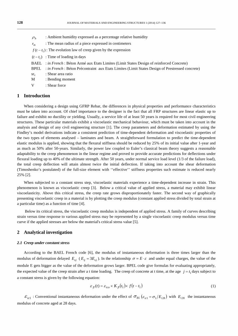
hρ : Ambient humidity expressed as a percentage relative humidity mr : The mean radius of a piece expressed in centimeters )( 1ttf − : The evolution law of creep given by the expression
)( 1tt − : Time of loading in days BAEL : in French : Béton Armé aux Etats Limites (Limit States Design of reinforced Concrete) BPEL : in French : Béton Précontraint aux Etats Limites (Limit States Design of Prestressed concrete) srz : Shear area ratio M : Bending moment V : Shear force
1 Introduction
When considering a design using GFRP Rebar, the differences in physical properties and performance characteristics must be taken into account. Of chief importance to the designer is the fact that all FRP structures are linear elastic up to failure and exhibit no ductility or yielding. Usually, a service life of at least 50 years is required for most civil engineering structures. These particular materials exhibit a viscoelastic mechanical behaviour, which must be taken into account in the analysis and design of any civil engineering structure [1]. The creep parameters and deformation estimated by using the Findley’s model derivations indicate a consistent prediction of time-dependent deformation and viscoelastic properties of the two types of elements analysed – laminates and beam. A straightforward formulation to predict the time-dependent elastic modulus is applied, showing that the flexural stiffness should be reduced by 25% of its initial value after 1-year and as much as 50% after 50-years. Similarly, the power law coupled to Euler’s classical beam theory suggests a reasonable adaptability to the creep phenomenon in the linear regime and proved to provide accurate predictions for deflections under flexural loading up to 40% of the ultimate strength. After 50 years, under normal service load level (1/3 of the failure load), the total creep deflection will attain almost twice the initial deflection. If taking into account the shear deformation (Timoshenko’s postulated) of the full-size element with ‘‘effective’’ stiffness properties such estimate is reduced nearly 25% [2].
When subjected to a constant stress step, viscoelastic materials experience a time-dependent increase in strain. This phenomenon is known as viscoelastic creep [3]. Below a critical value of applied stress, a material may exhibit linear viscoelasticity. Above this critical stress, the creep rate grows disproportionately faster. The second way of graphically presenting viscoelastic creep in a material is by plotting the creep modulus (constant applied stress divided by total strain at a particular time) as a function of time [4].
Below its critical stress, the viscoelastic creep modulus is independent of applied stress. A family of curves describing strain versus time response to various applied stress may be represented by a single viscoelastic creep modulus versus time curve if the applied stresses are below the material's critical stress value [5].
2 Analytical investigation
2.1 Creep under constant stress
According to the BAEL French code [6], the modulus of instantaneous deformation is three times larger than the modulus of deformation delayed jEυ ( jij EE υ3= ). In the relationship εσ ⋅= E and under equal charges, the value of the
module E gets bigger as the value of the deformation grows larger. BPEL code give formulas for evaluating appropriately, the expected value of the creep strain after a t time loading. The creep of concrete at t time, at the age 1tj = days subject to a constant stress is given by the following equation:
( ) ( )11)( ttftKt flicofl −××= εε (1)
1icε : Conventional instantaneous deformation under the effect of 1bσ ( )2811 iic Eσε = with 28iE the instantaneous
modulus of concrete aged at 28 days.
JOURNAL OF MATERIALS AND ENGINEERING STRUCTURES 1 (2014) 127–136 129
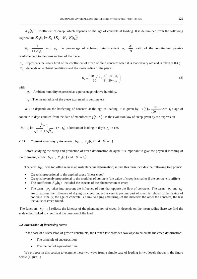
( )1tK fl : Coefficient of creep, which depends on the age of concrete at loading. It is determined from the following
expression: ( ) ( )( )11 tKKKKtK cesfl ⋅+⋅=
ssK
ρ2011
+= with sρ the percentage of adherent reinforcement
BAs
s =ρ , ratio of the longitudinal passive
reinforcement to the cross section of the piece
eK : represents the lower limit of the coefficient of creep of plain concrete when it is loaded very old and is taken at 0,4 ;
cK : depends on ambient conditions and the mean radius of the piece:
+−
+−
=m
hhc r
K20
10032
30120 ρρ (2)
with hρ : Ambient humidity expressed as a percentage relative humidity,
mr : The mean radius of the piece expressed in centimeters
( )1tK : depends on the hardening of concrete at the age of loading, it is given by: ( )1
1 100100
ttK
+= with 1t : age of
concrete in days counted from the date of manufacture ( )1ttf − : is the evolution law of creep given by the expression
( )mrtt
ttttf
51
11
+−
−=− : ( )1tt − : duration of loading in days; mr in cm.
2.1.1 Physical meaning of the words: 1icε , ( )1tK fl and ( )1ttf −
Before studying the creep and prediction of creep deformation delayed it is important to give the physical meaning of
the following words: 1icε , ( )1tK fl and ( )1ttf −
The term 1icε was too often seen as an instantaneous deformation; in fact this term includes the following two points:
• Creep is proportional to the applied stress (linear creep) • Creep is inversely proportional to the modulus of concrete (the value of creep is smaller if the concrete is stiffer) • The coefficient ( )1tK fl included the aspects of the phenomenon of creep
• The term sρ takes into account the influence of bars that oppose the flow of concrete. The terms hρ and mr are to express the influence of drying on creep, indeed a very important part of creep is related to the drying of concrete. Finally, the age of concrete is a link to aging (maturing) of the material: the older the concrete, the less the value of creep found.
The function ( )1ttf − reflects the kinetics of the phenomenon of creep. It depends on the mean radius (here we find the scale effect linked to creep) and the duration of the load.
2.2 Succession of increasing stress
In the case of a succession of growth constraints, the French law provides two ways to calculate the creep deformation:
• The principle of superposition
• The method of equivalent time
We propose in this section to examine these two ways from a simple case of loading in two levels shown in the figure below (Figure 1)

130 JOURNAL OF MATERIALS AND ENGINEERING STRUCTURES 1 (2014) 127–136
Fig. 1 – Schematic diagram of testing arrangement
2.2.1 Principle of superposition
In the case of loading as showed in Figure 2, the strain response is obtained by superposing the effects of each stress range.
Fig. 2 – Two stage simple loading
2.2.1.1 Expression of the creep deformation
The expression of creep deformation will be developed in the particular case of two levels and in the general case of n constraints marked shortening ∆σi with i ranging from 1 to n.
The principle of superposition implies that the deformation response is obtained by superposing the effects of each stress range. This can result graphically as shown in Figure 3.
Fig. 3 – Stress response by effects superposition
σ
Time t1
σ2
σ1
t2
σ
t1
σ2
σ1
Time t2
=
t1
σ1
σ
Time t2
+
σ2 – σ1
σ
Time t2

JOURNAL OF MATERIALS AND ENGINEERING STRUCTURES 1 (2014) 127–136 131
In terms of delayed deformation, the response deformation by superposition effects is shown in Fig 4.
Fig. 4 – Response deformation by superposition effects Therefore
( ) ( )2212
111
)( .)(..)(. ttftKE
ttftKE fllftfl −
−+−=
σσσε (3)
Generalizing to the case of n increased stress, creep deformation can be written
( )jjlf
n
jjtfl ttftK −∆=∑
=.)(.
1)( εε
2.2.1.2 Calculation of the delayed deformation of the concrete after 300 days 1000 and 3000 days
Numerical application for n=2 using data in Table 1
Table 1: Data for calculating the effect superposition
t1 (days)
t2 (days)
σ1 (MPa)
σ2 (MPa)
Ei 28 (Mpa) hρ
mr
(cm) sρ
8 28 8 16 32000 70 36 0.02
( )( )jcsfl tKKKK ⋅+⋅= 4,0
7143,0
2011
=+
=s
sKρ
024,2
20100
32
30120
=
+−
⋅+−
=m
hhc r
K ρρ
( )
jttK
+=
100100
0
624,1)8( =flK 415,1)28( =flK
mfl
mlf
otfl
rtt
tttK
Ertt
tttK
E 5.)(.
5.)(.
1
11
12
1
01)(
+−
−−+
+−
−=
σσσε
t= 300 j mmfl /8,272)300( µε =
t= 1000 j mmfl /4,387)1000( µε =
t= 3000 j mmfl /4,490)3000( µε =
t1
εfl
Time t2 1

132 JOURNAL OF MATERIALS AND ENGINEERING STRUCTURES 1 (2014) 127–136
2.2.2 Equivalent time
This method can be reduced for the assessment of creep, a single load in place of two successive loads. The time equivalent corresponds to the time at which a fictitious creep test performed under a constant stress equal to the current stress reaches the current deformation.
2.2.2.1 Equations of equivalent time and creep deformation
The response strength by equivalent is shown in Figure 5 for t > t2 . Graphical view the equivalent time is such that we have, for t > t2. For the answer deformation we get the following mapping as shown in Figure 5:
Fig. 5 – Response strength by equivalent time
The equivalent time is given by the equation:
( ) ( )).)(..)(. 22
1211
)( 2 eqeqfllftfl tfttKE
ttftKE
−=−=σσ
ε (4)
Creep deformation for t > t2 :
( )eqéqfltfl tttfttKE
+−−= 222
)( .)(.σε
2.2.2.2 Equations in the general case of n greater strength
The equations in the general case of n greater strength noted ∆σi with i variant from 1 to n and t in the range of time [ti , ti+1] can be expressed:
t ϵ c [ti , ti+1] ( )éqiiiéqifli
tfl tttfttKE
+−−= .)(.)(σε
with ( )éqiiéqifli
tifl tfttKE
.)(.)( −=σ
ε
2.2.2.3 After the second equivalent time loading (t > t2)
The same data is determinate as before (numerical Application for n = 2 of paragraph 2.2.1 a) , the equivalent time after the second loading (t > t1) and then calculate the creep strain after 300 days and 3000 days.
)828(.)8(.
320008
)28( −= fK flflε
( )eqiieqflfl tftK .)28(.
320008
)28( −=ε
t1
σ2
σ1
σ
Time t2
=
σ2
σ
Time t2
t eq
JOURNAL OF MATERIALS AND ENGINEERING STRUCTURES 1 (2014) 127–136 133
By iteration we get: 28 – t eq = 22,6 t eq = 5,4 days
t = 300 days mmfl /6,261)300( µε =
t = 3000 days mmfl /473)3000( µε =
Comments
- These values are close to those calculated by the principle of superposition. We recall also that a deformation is a no unit magnitude.
- In the case of real load, the calculation by the method of superposition implies remembering all the steps of charges. This method is expensive computation in time and memory. The interest of the equivalent time method is to avoid these disadvantages since it requires only the current state of stress and strain.
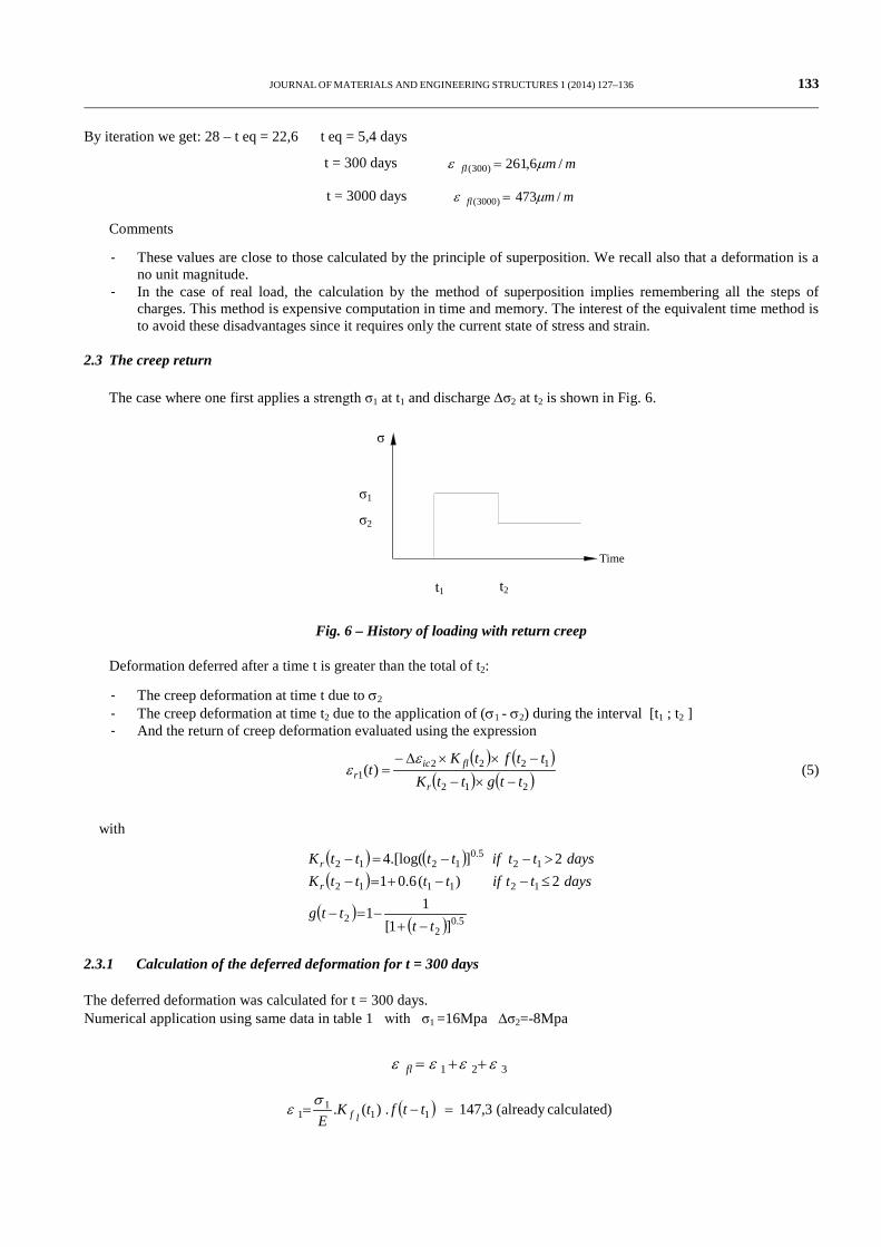
2.3 The creep return
The case where one first applies a strength σ1 at t1 and discharge ∆σ2 at t2 is shown in Fig. 6.
Fig. 6 – History of loading with return creep
Deformation deferred after a time t is greater than the total of t2:
- The creep deformation at time t due to σ2 - The creep deformation at time t2 due to the application of (σ1 - σ2) during the interval [t1 ; t2 ] - And the return of creep deformation evaluated using the expression
( ) ( )
( ) ( )212
12221 )(
ttgttKttftK
tr
flicr −×−
−××∆−=
εε (5)
with
( ) ( )( )
( )( ) 5.0
22
121112
125.0
1212
]1[11
2)(6.012].[log(4
ttttg
daysttifttttKdaysttifttttK
r
r
−+−=−
≤−−+=−>−−=−
2.3.1 Calculation of the deferred deformation for t = 300 days
The deferred deformation was calculated for t = 300 days. Numerical application using same data in table 1 with σ1 =16Mpa ∆σ2=-8Mpa
321 εεεε ++=fl
( ) )calculatedalready (3,147.)(. 111
1 =−= ttftKE lfσ
ε
Time
t1
σ
σ1
σ2
t2
134 JOURNAL OF MATERIALS AND ENGINEERING STRUCTURES 1 (2014) 127–136
( ) )calculatedalready (7,52.)(. 12121
2 =−−
= ttftKE lfσσ
ε
( )( ) ( ) 5,9.
()(. 2
12
121
123 −=−
−−−
= ttgttKr
ttftKE lf
σσε
mmfl /5,190)300( µε =
With the superposition principle:
mmKlf /7,294
8300308300.)8(.
3200016
1 µε =−+
−=
mmKlf /5,125
8300308300.)28(.
320008
2 µε −=−+
−−=
mm /2,16921 µεεε =+=
2.3.2 Results comparison
The results obtained at t = 300 days by BPEL law will be compared to a strict application of the superposition principle (using the same law for the loading and unloading). We observe what was predictable, that the superposition principle in this case conducted to a much lower final deformation (which corresponds to a stronger return). The formulas give a return of creep deformation of lower order to take into account this aspect: the return of creep of concrete is by far the symmetric flow.
2.4 Reloading
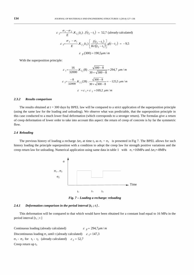
The previous history of loading a recharge ∆σ2 at time t3 as σ1 = σ3 is presented in Fig 7. The BPEL allows for such history loading the principle superposition with a condition to adopt the creep law for strength positive variations and the creep return law for unloading. Numerical application using same data in table 1 with σ1 =16MPa and ∆σ2=-8MPa
Fig. 7 – Loading a recharge: reloading
2.4.1 Deformation comparison in the period interval [t1 ; t ] .
This deformation will be compared to that which would have been obtained for a constant load equal to 16 MPa in the period interval [t1 ; t ]
Continuous loading (already calculated) mmfl /7,294 µε =
Discontinuous loading σ1 until t (already calculated) 3,1471=ε σ1 - σ2 for t1 - t2 (already calculated) 7,522 =ε Creep return up t3
t1
σ1 = σ3
σ2
σ
Time t2
t3
JOURNAL OF MATERIALS AND ENGINEERING STRUCTURES 1 (2014) 127–136 135
( )( ) ( ) 8,7.
()28(.
320008
2312
1203 −=−
−−−
= ttgttKr
ttfKlfε
σ1 - σ3 de t3 à t :
( ) 9,12429300.)29(.32000
84 =−= fK
lfε
mmfl /1,3174321 µεεεεε =+++=
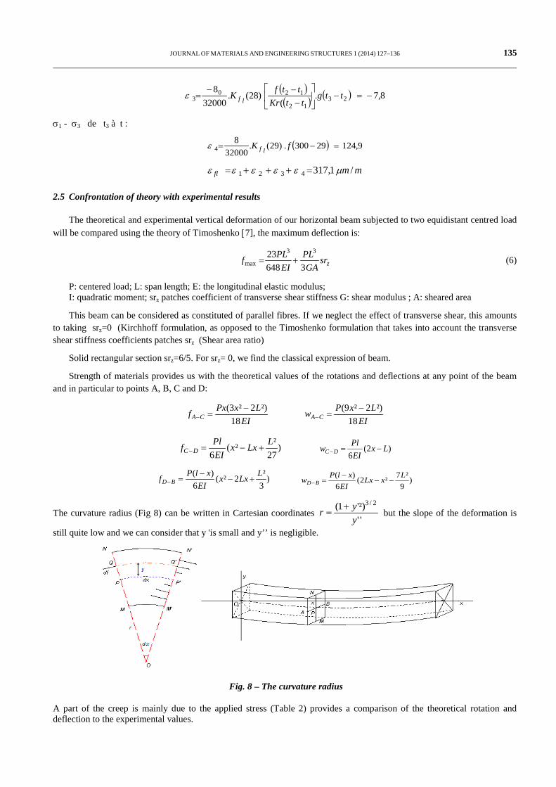
2.5 Confrontation of theory with experimental results
The theoretical and experimental vertical deformation of our horizontal beam subjected to two equidistant centred load will be compared using the theory of Timoshenko [7], the maximum deflection is:
zsrGA
PLEI
PLf3648
23 33
max += (6)
P: centered load; L: span length; E: the longitudinal elastic modulus; I: quadratic moment; srz patches coefficient of transverse shear stiffness G: shear modulus ; A: sheared area
This beam can be considered as constituted of parallel fibres. If we neglect the effect of transverse shear, this amounts to taking srz=0 (Kirchhoff formulation, as opposed to the Timoshenko formulation that takes into account the transverse shear stiffness coefficients patches srz (Shear area ratio)
Solid rectangular section srz=6/5. For srz= 0, we find the classical expression of beam.
Strength of materials provides us with the theoretical values of the rotations and deflections at any point of the beam and in particular to points A, B, C and D:
EI
LxPxf CA 18²)2²3( −
=− EI
LxPw CA 18²)2²9( −
=−
)
27²²(
6LLxx
EIPlf DC +−=− )2(
6Lx
EIPlw DC −=−
)
3²2²(
6)( LLxx
EIxlPf BD +−
−=− )
9²7²2(
6)( LxLx
EIxlPw BD −−
−=−
The curvature radius (Fig 8) can be written in Cartesian coordinates ''
'²)1( 2/3
yyr +
= but the slope of the deformation is
still quite low and we can consider that y 'is small and y’’ is negligible.
Fig. 8 – The curvature radius
A part of the creep is mainly due to the applied stress (Table 2) provides a comparison of the theoretical rotation and deflection to the experimental values.
136 JOURNAL OF MATERIALS AND ENGINEERING STRUCTURES 1 (2014) 127–136
Table 2 Comparison of the theoretical rotation and deflection to the experimental values (P=500daN)
Age j
( days)
Deflection (mm) Rotation (mm²) C D A B C D
EIPL
1625 3
EIPL
1625 3
EIPL9
2
EIPL9
2
− EI
PL18
2
EIPL
18
2
−
Experimental Value
0
F i* 0,765 0,742 8,371 -8.132 4,163 -4,068 Fv** 0 0 total 0,765 0,742 8,371 -8,132 4,163 -4,068
300
F i* 0,765 0,742 8,371 -8,132 4,163 -4,068 Fv** 1,731 13,532 -12,961 7,157 -7,364 total 2,496 2,473 21,903 -21,093 11,32 -11,432
Theoretical Value
0
F i* 1,359 1,359 14,82 -14,82 7,41 -7,41 Fv** 0 0 total 1,359 1,359 14,82 -14,82 7,41 -7,41
300
F i* 1,359 1,359 14,82 -14,82 7,41 -7,41 Fv** mmfl /8,272)300( µε =
- - - -
total 1,359 1,359 14,82 -14,82 7,41 -7,41 * immediate ** creep deflection
Conclusion
After having explained the experimental study (presented and discussed in Part A), Part B of the present paper focused on the analytical investigations intended to calibrate existing formulas by means of the strain and deflection measurements obtained in the experimental tests. The following recommendations and conclusions are drawn from this study:
- The method of superposition principle is expensive computation in time and memory. The interest of the equivalent time method is to avoid these disadvantages since it requires only the current state of stress and strain
- The superposition principle conducted to a much lower final deformation (which corresponds to a stronger return). The creep return of concrete is by far the symmetrical creep.
- The BPEL allows when we used a loading-unloading cycle, the use of principle superposition but with different laws in loading and unloading cycle.
- The purpose of the numerical application is to show an overestimation of creep deformation (effect we do not have with the time equivalent method). In the limit by succession of very short loading -unloading cycles application of BPEL led to grossly overestimated deformations.
Acknowledgments The authors would like to thank the manufacturer of the GFRP Combar (Schöck, Baden-Baden, Germany) for
providing and supporting this research. The opinion and analysis presented in this paper are those of the authors.
REFERENCES
[1]- M.F. Sá, Mechanical and structural behaviour of FRP – Pultruded GFRP elements. Master’s Thesis in Structural Engineering. IST, Technical University of Lisbon, in Portuguese, 2007
[2]- M.F. Sá, A.M. Gomes, J.R. Correia, N. Silvestre, Creep behavior of pultruded GFRP elements – Part 2: Analytical study, Compos. Struct. 93(9)(2011) 2409-2418
[3]- B. Benmokrane, O. Chaallal, R. Masmoudi Flexural response of concrete beams reinforced with FRP Reinforceing bars. ACI Struct J. 93(1)(1996) 46–55.
[4]- Schock Bauteil GmbH Combar, Design Guideline for Concrete Structures Reinforced with Glass Fiber Reinforced Polymer following the Requirements of DIN 1045-1and EC2 Issued Germany, 2006
[5]- R. Aboutaha, Recommended Design for the GFRP Rebar Combar, Syracuse University, Department of Civil and Environmental Engineering, Technical Report, USA, 2004.
[6]- BAEL 1983 : Reglement de calcul du béton armé aux états limites [7]- W. Weaver, S.P. Timoshenko, D.H. Young, Vibrations Problems in Engineering, Wiley and Sons, 4th Ed., 1974

JOURNAL OF MATERIALS AND ENGINEERING STRUCTURES 1 (2014) 137–145
137
Research Paper
Buckling Response of Thick Functionally Graded Plates
Mokhtar Bouazza *,1,2, Abedlouahed Tounsi 2, EL Abbas Adda-Bedia 2 1 Department of Civil Engineering, University of Béchar, Béchar 08000, Algeria. 2 Laboratory of Materials and Hydrology (LMH), University of Sidi Bel Abbès, Sidi Bel Abbès 2200, Algeria.
A R T I C L E I N F O
Article history :
Received : 15 July 2014
Revised : 16 November 2014
Accepted : 18 November 2014
Keywords:
Thermal buckling
Functionally graded material
FSDT
CPT
A B S T R A C T
In this paper, the buckling of a functionally graded plate is studied by using first order shear deformation theory (FSDT). The material properties of the plate are assumed to be graded continuously in the direction of thickness. The variation of the material properties follows a simple power-law distribution in terms of the volume fractions of constituents. The von Karman strains are used to construct the equilibrium equations of the plates subjected to two types of thermal loading, linear temperature rise and gradient through the thickness are considered. The governing equations are reduced to linear differential equation with boundary conditions yielding a simple solution procedure. In addition, the effects of temperature field, volume fraction distributions, and system geometric parameters are investigated. The results are compared with the results of the no shear deformation theory (classic plate theory, CPT).
1 Introduction
The idea of the construction of functionally graded materials (FGMs) was first introduced in 1984 by a group of Japanese materials scientists [1, 2]. During the past two decades, FGMs have experienced a noteworthy increase in terms of research and development programs. World wide distribution and dissemination of the results through publications, international meetings and exchange programs testifies to this increasing growth. They have many gained applications in rocket engine components, space plan body, nuclear reactor components, first wall of fusion reactor, engine components, turbine blades, hip implant and other engineering and technological applications. A detailed discussion on their design, processing and applications can be found in [3]. FGMs are also promising candidates for future intelligent composites [4]. They are multifunctional composite materials, mechanical properties of which vary smoothly and continuously from one side to the other. This is achieved by a continuous change in composition of the constituent materials.
* Corresponding author. +213662137302/ +213662462737 E-mail address: [email protected] e-ISSN: 2170-127X, © Mouloud Mammeri University of Tizi-Ouzou, Algeria

138 JOURNAL OF MATERIALS AND ENGINEERING STRUCTURES 1 (2014) 137–145
The most well-known FGM is compositionally graded from a ceramic to a metal to incorporate such diverse properties as heat, wear and oxidation resistance of ceramics with the toughness, strength, machinability and bending capability of metals.
Buckling and post-buckling characteristics are one of the major design criteria for plates/panels for their optimal usage. Hence, it is, therefore, important to study the buckling and post-buckling characteristics of FGM plates under mechanical, thermal or thermo-mechanical loading for accurate and reliable design. The buckling of rectangular plates has been the subject of study for many investigators during the past. However, investigations on the post-buckling behavior of FGM plates are rather limited in number. Praveen and Reddy [5] investigated the response of functionally graded ceramic-metal plate, using finite element procedure. Reddy [6] presented the theoretical and finite element formulations for linear and nonlinear thermomechanical response of FGM plates employing higher order shear deformation theory. Javaheri and Eslami [7,8] obtained the buckling of the FGM plate for uniform in-plane compressive loading and thermal loading using variational approach, based on classical plate theory. They employed equilibrium and stability relations to study the buckling behavior of functionally graded plates with all edges simply supported. Vel and Batra [9] found an exact solution for the thermoelastic deformation of functionally graded thick rectangular simply supported plates. Yang and Shen [10] presented a semi-numerical approach for nonlinear bending analysis of shear deformable functionally graded plates subjected to thermo-mechanical loads, incorporating Reddy's higher order shear deformation theory.
Employing Galerkin-differential quadrature iteration based scheme and incorporating Reddy's higher order shear deformation theory, Liew et al. [11] investigated the postbuckling behavior of the piezoelectric FGM plate. Using Fourier series, Woo et al. [12] presented an analytical solution based on mixed Fourier series for post-buckling of functional graded material plates and shallow cylindrical shells under thermo-mechanical loading. Ma and Wang [13] presented the relationships between axisymmetric bending and buckling of FGM circular plate. Bouazza et al [14] obtained the closed form solution for the thermal buckling of sigmoid functionally graded rectangular simply supported plates subjected to three types of temperature fields; uniform temperature rise; linear temperature rise and sinusoidal temperature rise, employing the first-order shear deformation theory. Shen [15] obtained the post-buckling response of axially loaded functionally graded cylindrical panels subjected to thermal loading. Based on Reddy's higher order shear deformation theory and von-Karman–Donnell type nonlinearity, Shen and Leung [16] presented the post-buckling analysis of functionally graded cylindrical panel under lateral pressure and temperature. Najafizadeh and Eslami [17] presented the buckling analysis of solid circular clamped and simply supported FGM plate. Based on classical plate theory, Yang and Shen [18] presented a semi-analytical approach for the large deflection and post-buckling response of a functionally graded rectangular plate with two opposite edges clamped and two simply supported and subjected to transverse and in-plane loads. Ma and Wang [19] investigated the axisymmetric thermal post-buckling behavior of a functionally graded circular plate.
The object of this investigation is to present an analytical solution for buckling of P-FGM plates subjected to linear temperature rise or non-linear temperature rise across the thickness. The material properties are assumed to be graded in the thickness direction according to a simple power-law distribution in terms of the volume fractions of the constituents. The FSDT and the von Karman-type linear strains are used to construct the problem governing equations. The effects of volume fraction index on the critical temperature buckling behavior are studied.
2 Theoretical Formulation
The functionally graded material (FGM) can be produced by continuously varying the constituents of multi-phase materials in a predetermined profile. The most distinct features of an FGM are the non-uniform microstructures with continuously graded properties. A FGM can be defined by the variation in the volume fractions. Most researchers use the power-law function, to describe the volume fractions.
2.1 P-FGM structures
In order to analyze P-FGM structures as shown in Fig. 1, the simple power-law distribution (Praveen and Reddy [5, 6]) can be employed in this study. The volume fraction using power-law functions to ensure smooth distribution of stresses is defined.

JOURNAL OF MATERIALS AND ENGINEERING STRUCTURES 1 (2014) 137–145 139
( )kf hzzV 2/1/)( += (1)
where h is the thickness of the plate and k is the material parameter that dictates the material variation profile through the thickness.
Fig. 1. Typical FGM square plate.
By using the rule of mixture, the material properties of the P-FGM can be calculated by [5, 8, 14]
0)(
)()(
)()(
νν
αααααα
=
−=+=
−=+=
z
zVz
EEEzVEEzE
mccmfcmm
mccmfcmm
(2)
where )(zE denotes a generic material property such as modulus, cE and mE indicate the property of the top and bottom faces of the structure, respectively.
2.2 Stability equations
Assume that wvu ,, denote the displacements of the neutral plane of the plate in x, y, z directions respectively;
yx φφ , denote the rotations of the normals to the plate midplane. According to the first order shear deformation theory, the
strains of the plate can be expressed [20-22]
yyzyxxxz
xyyxxyxy
yyyyxxxx
ww
zu
zzu
,,
,,,,
,,,,
)(
+=+=
+++=
+=+=
φγφγ
φφυγ
φυεφε
(3)
The forces and moments per unit length of the plate expressed in terms of the stress components through the thickness are
∫∫∫−−−
===2/
2/
2/
2/
2/
2/
;;h
hijij
h
hijij
h
hijij dzQdzzMdzN τσσ (4)
The nonlinear equations of equilibrium according to Von Karman’s theory are given by:
02
02
02
,,,,,
,,,,
,,,
=+++++
=−−+
=++
xyxyyyyxxxyyxx
yyxxxyxyxxx
yyyxyxyxxx
wNwNwNqQQ
QQMM
NNN (5)
Using Eqs.(2), (3) and (4), and assuming that the temperature variation is non-uniform with respect to x- and y-directions, the equilibrium Eq. (5) may be reduced to a set of one equation as

140 JOURNAL OF MATERIALS AND ENGINEERING STRUCTURES 1 (2014) 137–145
0)2()1(
)2()1(2
,,,2231
21
,,,2
1
4
=+++−−
−
+++∇+
+∇
qwNwNwNEEE
E
qwNwNwNE
w
xyxyyyyxxx
xyxyyyyxxx
ν
ν
(6)
where
∫−
=2/
2/
2321 )(),,1(),,(
h
h
dzzEzzEEE (7)
∫−
=ΘΦ2/
2/
),,()()(),1(),(h
h
dzzyxTzzEz α (8)
To establish the stability equations, the critical equilibrium method is used. Assuming that the state of stable equilibrium of a general plate under thermal load may be designated by 0w . The displacement of the neighboring state
is 10 ww + , where 1w is an arbitrarily small increment of displacement. Substituting 10 ww + into Eq. (6) and
subtracting the original equation, results in the following stability equation
0)2()1(
)2()1(2
,10
,10
,10
2231
21
,10
,10
,102
11
4
=++−
−−
++∇+
+∇
xyxyyyyxxx
xyxyyyyxxx
wNwNwNEEE
E
wNwNwNE
w
ν
ν
(9)
where, 000 , xyyx NandNN refer to the pre-buckling force resultants
To determine the buckling temperature difference crT∆ , the pre-buckling thermal forces should be found firstly.
Solving the membrane form of equilibrium equations, gives the pre-buckling force resultants:
0,1
,1
000 =−Φ
−=−Φ
−= xyyx NNNνν
(10)
Substituting Eq(9) into Eq. (8), one obtains
01
)1(1
)1(21
22231
21
14
11
4 =∇−Φ
−
−+∇
−Φ+
−∇ wEEE
EwE
wν
νν
ν (11)
The simply supported boundary condition is defined as
byonMw
axonMw
xy
yx
,00,0,0
,00,0,0
111
111
====
====
φ
φ (12)
The following approximate solution is seen to satisfy both the governing equation and the boundary conditions
)/(sin)/(sin1 bynaxmcw ππ= (13)
where m, n are number of half waves in the x and y directions, respectively, and c is a constant coefficient.
3 Buckling Analysis
In this section, the thermal buckling behaviors of simply supported square metal-ceramic plates under thermal environment are analyzed. The thermal load is assumed to be linear temperature rise and nonlinear temperature change through the thickness direction. The reference temperature is assumed to be 5°C. The effects of volume fraction index and geometric parameter a/h are investigated in each case.

JOURNAL OF MATERIALS AND ENGINEERING STRUCTURES 1 (2014) 137–145 141
3.1 Linear temperature rise
The temperature field under linear temperature rise through the thickness is assumed as
mThzhTzT ++
∆= )2/()( (14)
where z is the coordinate variable in the thickness direction which measured from the middle plane of the plate.
mT is the metal temperature and T∆ is the temperature difference between ceramic surface and metal surface, i.e., mc TTT −=∆ . For this loading case, the thermal parameter Φ can be expressed as
TXTP m ∆+=Φ (15)
where
)22()2(
)(2 +
++
++=
khE
khEEhEX mcmcmmcmcmmm αααα
(16)
From Eq.(15) one has
X
TPT mcr
−Φ=∆ (17)
3.2 Nonlinear temperature change
The functionally graded materials are designed in order to resist high temperature rise by ceramic, so the temperature change will be quite different at the two sides of the FGM structures. When the temperature rises differently at the inner and outer surfaces of the plate, the temperature distribution across the thickness is governed by the steady state heat conduction equation and boundary condition as follows:
( ) ( ) ( ) mc ThTThTdzdTzK
dzd
=−==
2,2,0 (18)
where ( )zK is the coefficient of thermal conduction. Similar to the elasticity and thermal expansion properties, we assume that the thermal conductive coefficient is also a power form function as
( ) ( ) mk
cm KhzKzK ++= 21 (19)
where
mccm KKK −= (20)
The solution of Eq. (18) is obtained by means of polynomial series. Taking the first seven terms of the series, the solution for temperature distribution across the plate thickness becomes [8]
( ) ηCTTzT m
∆+= (21)
with
( )( )( )
∑∞=
= +
+−+=
n
n
nmcm
k
nk
KKzz
0 1
2121η (22)
( )
∑∞=
= +
−=
n
n
nmcm
nk
KKC
0 1 (23)
where mc TTT −=∆ is defined as the temperature difference between ceramic-rich and metal-rich surfaces of the plate. Substituting Eq. (21) into the thermal parameter equation (8), yields

142 JOURNAL OF MATERIALS AND ENGINEERING STRUCTURES 1 (2014) 137–145
THPTm ∆+=Φ (24)
where
( )
( )∑
∑
∞=
=
∞=
=
+
−
+++
+++
+++
−
=n
n
nmcm
cmcmmcmcmmmmn
n
nmcm
nkKK
knE
knEE
nkE
nkKK
hH
0
0
1
2)2(2)1(21αααα
(25)
From Eq. (24) one has
HPTT m
cr−Φ
=∆ (26)
The critical temperature difference is obtained for the values of m=n=1.
4 Numerical Results and Discussion
Based on the derived formulation, a computer program is developed to study the behavior of P-FGM plates in thermal buckling. The analysis is performed for pure materials and different values of volume fraction exponent, k, for aluminum–alumina FGM. The Young’s modulus and Poisson’s ratio for aluminum are: 70 GPa and 0.3 and for alumina: 380GPa and 0.3, respectively. Note that the Poisson’s ratio is chosen to be 0.3 for simplicity. Fig. 2 depicts the variation of the Young's modulus through the thickness with different values of volume fraction exponent k .
-0.5 -0.4 -0.3 -0.2 -0.1 0.0 0.1 0.2 0.3 0.4 0.550
100
150
200
250
300
350
400
k=0.3 k=1 k=3 k=5 k=10
Youn
g’s
mod
ulus
z/h
Fig 2. Young’s modulus variation associated with different exponent indexes for a P-FGM plate.
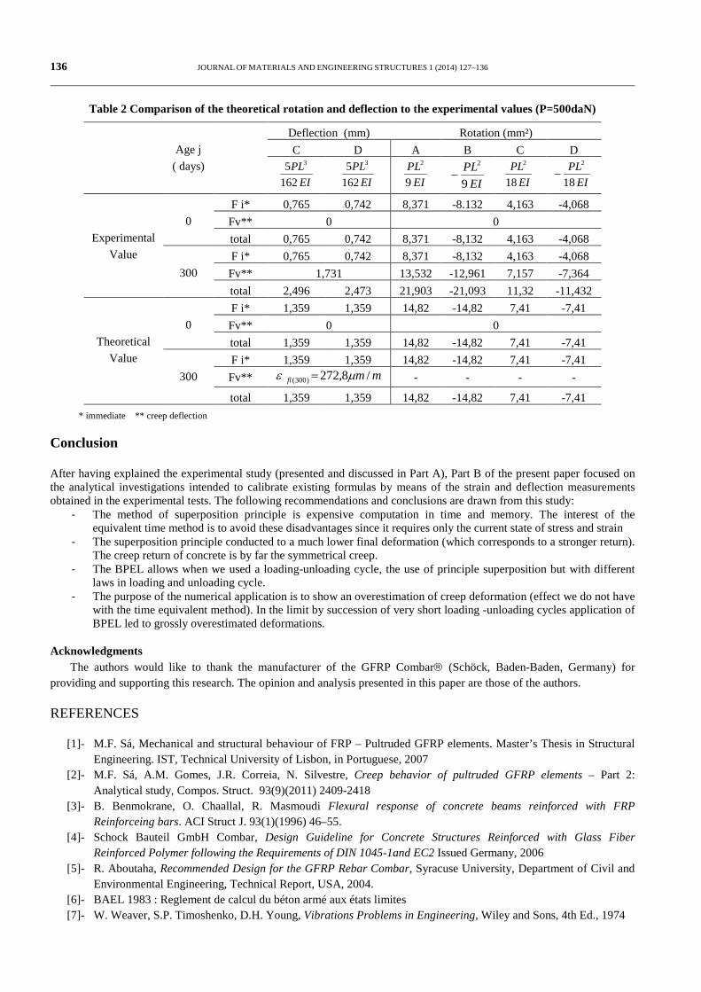
The variation of the critical temperature change crT∆ of alumina-aluminium FGM plates under linear temperature rise for two different geometric parameters and volume fraction index are plotted in Fig. 3. The isotropic alumina and aluminium cases correspond to fully ceramic plates and fully metallic plates, respectively. While the other cases,
5,1,3.0=k , are for the graded plates with two constituent materials.
In Fig. 3, it is found that the critical temperature change of FGM plates is higher than that of the fully metal plates but lower than that of the fully ceramic plates. In addition, the critical temperature change decreases as volume fraction index k is increased. This is because for FGMs, as the volume fraction index is increased, the contained quantity of metal increases. In all material cases, the critical temperature change decreases, when the geometric parameter a/h is increased. The responses are very similar comparing to of sigmoid functionally graded plates (Bouazza et al. [14]).
JOURNAL OF MATERIALS AND ENGINEERING STRUCTURES 1 (2014) 137–145 143
2 4 6 8 10 12 14 16 18 20
0
5000
10000
15000
20000
25000
30000
35000
40000 P-FGM Linear temperature changea/b=1
Alumina k=0.3 k=1 k=3 Aluminium
Critic
al te
mpe
ratu
re (°
C)
a/h
Fig.3. Critical temperature gradient as a function of the side-to-thickness ratio (a/h) of a P-FGM square plate, under linear temperature rise.
2 4 6 8 10 12 14 16 18 20
0
10000
20000
30000
40000
50000
60000
k=0.3
P-FGM Linear temperature changea/b=1
FSDT CPT
Critic
al te
mpe
ratu
re (°
C)
a/h
Fig.4. Comparison between temperature graphs vs. ratio Ah (a/h) based on first order shear deformation theory, classic plate theory in the case of linear temperature rise with square plate, k=0.3.
2 4 6 8 10 12 14 16 18 20-5000
0
5000
10000
15000
20000
25000
30000
35000
40000
k=1
P-FGM Linear temperature changea/b=1
FSDT CPT
Critic
al te
mpe
ratu
re (°
C)
a/h
Fig.5. Comparison between temperature graphs vs. ratio Ah (a/h) based on first order shear deformation theory, classic plate theory in the case of linear temperature rise with square plate, k=1.

144 JOURNAL OF MATERIALS AND ENGINEERING STRUCTURES 1 (2014) 137–145
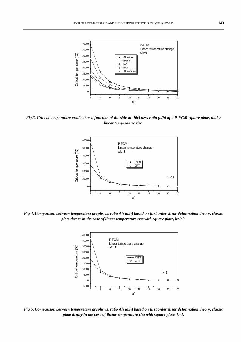
In Figs. 4-6 the graphs of results of thermal buckling analysis for the P-FGM based on the FSDT compared to CPT are presented. These figures show that the buckling temperature increases by the decreases of the ratio a/h. In addition, based on the figures, the results obtained by first order shear deformation theory coincide with the results of classic plate theory. This is well explained by the large plate aspect ratio a/h=10, 20 or the small plate thickness h
2 4 6 8 10 12 14 16 18 20
0
4000
8000
12000
16000
20000
24000
28000
32000
k=5
P-FGM Linear temperature changea/b=1
FSDT CPT
Critic
al te
mpe
ratu
re (°
C)
a/h
Fig.6. Comparison between temperature graphs vs. ratio Ah (a/h) based on first order shear deformation theory, classic plate theory in the case of linear temperature rise with square plate, k=5.
0 1 2 3 4 5
1000
1500
2000
2500
3000
3500
P-FGMFSDTa/h=10a/b=1Tm=5°C
Linear temperature rise Non linear temperature rise
Critic
al te
mpe
ratu
re (°
C)
k
Fig. 7. Critical buckling temperature rise of a functionally graded square plate vs k (a/h=10).
Fig. 6 shows the buckling temperature vs the material gradient exponent k for a plate with a/h =10, a/b= 1. We can see that the critical buckling temperature for a homogeneous ceramic square with 0=k is considerably higher than those for the functionally graded squares with 0≥k . It is evident that the buckling temperature decreases as the material volume fraction exponent k increases monotonically. As the gradient index k changes from 0 to 1, the critical buckling temperature decreases significantly. When k changes from 1 to 2, it reduces very slowly, and as k becomes larger than 2, it will be a constant practically. However, the critical temperature gradient under non-linear temperature rise is higher than that linear temperature rise.
5 Conclusion
In the present paper, equilibrium and stability equations of rectangular functionally graded plates are derived. Derivations are based on the First order shear deformation theory and the P-FGM the constituent materials. The buckling

JOURNAL OF MATERIALS AND ENGINEERING STRUCTURES 1 (2014) 137–145 145
analysis of such plates under linear thermal loads or nonlinear temperature change is investigated. The followings are concluded:
- Thermal buckling analysis decreases, as geometric parameter a/h is increased.
- Tcr of a functionally graded plate increases with the decreased of power law index k .
- Transverse shear deformation has considerable effect on the critical buckling temperature difference of functionally graded plate, especially for a thick plate or a plate with large aspect ratio.
- The critical temperature gradient under non-linear temperature rise is higher than that under linear temperature rise
REFERENCES
[1]- M. Yamanouchi, M. Koizumi, T. Hirai, I. Shiota, On the design of functionally gradient materials, In: Proceedings of the first international symposium on functionally gradient materials. Sendai, Japan, pp. 5-10, 1990.
[2]- M. Koizumi, The concept of FGM. Ceramic Transactions: Functionally Graded Materials 34(1993) 3–10. [3]- Y. Miyamoto, W.A. Kaysser, B.H. Rabin, A. Kawasaki, R.G. Ford, Functionally graded materials: design,
processing and applications. Kluwer Academic Publishers, 1999. [4]- J.S. Moya, Layered ceramics. Adv. Mater. 7(1995) 185–189. [5]- G.N. Praveen, J.N. Reddy, Nonlinear transient thermoelastic analysis of functionally graded ceramic-metal plates.
Int. J. Solids Struct. 35(33)(1998) 4457–4476. [6]- J.N. Reddy, Analysis of functionally graded plates. Int. J. Numer. Meth. Eng. 47(2000) 663–684. [7]- R. Javaheri, M.R. Eslami, Buckling of functionally graded plates under in-plane compressive loading. ZAMM-J.
Appl. Math. Mech. 82(4)(2002) 277–283. [8]- R. Javaheri, M.R. Eslami, Thermal buckling of functionally graded plates. AIAA J.; 40(1)(2002) 162–169. [9]- S.S. Vel, R.C. Batra, Exact solution for thermoelastic deformations of functionally graded thick rectangular plates.
AIAA J. 40(7)(2002) 1421–1433. [10]- J. Yang, H.S. Shen, Nonlinear bending analysis of shear deformable functionally graded plates subjected to
thermo-mechanical loads under various boundary conditions. Compos. Part B-Eng. 34(2)(2003) 103–115. [11]- K.M. Liew, J. Yang, S. Kittipornchai, Postbuckling of piezoelectric FGM plates subjected to thermo-electro-
mechanical loading. Int. J. Solids Struct. 40(15)(2003) 3689–3892. [12]- J. Woo, S.A. Meguid, K.M. Liew, Thermomechanical postbuckling analysis of functionally graded plates and
shallow cylindrical shells. Acta Mech. 165(1–2)(2003) 99–115. [13]- L.S. Ma, T.J. Wang, Relationship between axisymmetric bending and buckling solution of FGM circular plates
based on third order plate theory and classical plate theory. Int. J. Solids Struct. 41(1)(2004) 85–101. [14]- M. Bouazza, A. Tounsi, E.A. Adda-Bedia, A. Megueni, Buckling Analysis of Functionally Graded Plates with
Simply Supported Edges. Leonardo J. Sci. (15)(2009) 21-32. [15]- H-S. Shen, Postbuckling of axially loaded functionally graded cylindrical panels in thermal environments. Int. J.
Solids Struct. 39(24)(2002) 5991–6010. [16]- H-S Shen, A.Y.T. Leung, Postbuckling of pressure-loaded functionally graded cylindrical panels in thermal
environments. J. Eng. Mech-ASCE. 129(4)(2003) 414–425. [17]- M.M. Najafizadeh, M.R. Eslami, Buckling analysis of circular plates of functionally graded materials under
uniform radial compression. Int. J. Mech. Sci. 44(12)(2002) 2474–2493. [18]- J. Yanga, H-S. Shen, Non-linear analysis of functionally graded plates under transverse and in-plane loads. Int. J.
Nonlinear Mech. 38(4)(2003) 467–82. [19]- L.S. Ma, T.J. Wang, Nonlinear bending and post-buckling of a functionally graded circular plate under
mechanical and thermal loadings. Int. J. Solids Struct. 40(2003) 3311–3330. [20]- R.D. Mindlin, Influence of Rotatory Inertia and Shear on Flexural Motions of Isotropic, Elastic Plates. J. Appl.
Mech. 18(1951) 31–38. [21]- E. Reissner, On the Theory of Bending of Elastic Plates. J. Math. Phy. 23(1944) 184–191. [22]- E. Reissner, The Effect of Transverse Shear Deformation on the Bending of Elastic Plates. J. Appl. Mech-T
ASME 12(1945) 68–77.
146 JOURNAL OF MATERIALS AND ENGINEERING STRUCTURES 1 (2014) 146–154
Research Paper
Détermination du point de performance des portiques en B.A par la méthode statique non linéaire pushover Determination of the performance point of reinforced concrete frames using the nonlinear static method pushover
El Ghoulbzouri Abdelouafi *,a, El Alami Zakaria a, El Hannoudi Sabrine a aGC/GE , ENSAH ,Université Mohammed Premier, Al Hoceima ,Maroc
A R T I C L E I N F O
Article history:
Received : 24 June 2014
Received : 12 October 2014
Accepted : 08 November 2014
Mots clés :
Analyse statique non linéaire
Point de performance
Rotule
Site
Keywords:
Nonlinear static analysis
Performance point
Hinge
Site
R E S U M E
Le but du présent travail consiste à déterminer le point de performance des portiques en mettant l’accent sur l’influence du site sur les dégâts observés, l’emplacement de ce point sur la courbe capacité permettra de prédire le comportement réel du bâtiment en cas de séismes. Cette méthode consiste dans une première étape à appliquer des charges statiques équivalentes d’allure triangulaire sur le portique étudié, le comportement non linéaire de la structure sera défini, la non linéarité de la structure est introduite au moyen de rotules plastiques de flexion et de cisaillement., La seconde étape consiste à trouver la courbe de capacité en transformant respectivement l’effort tranchant à la base et le déplacement du sommet de l’analyse push over à l’accélération et le déplacement correspondant à un système à un seul degré de liberté, finalement les résultats seront discutés.
A B S T R A C T
The purpose of this work is determination of the performance point of a frame for different soil type, the location of this point on the curve capacity will predict the behavior of the frame in case of earthquakes, this method consists in a first step to apply static loads on the frame, the non linear behavior of the structure is defined, the nonlinearity of the structure is introduced with the use of plastic hinges, the second step is to find the capacity curve by transforming respectively shear at the base and displacement in the top to acceleration and displacement corresponding to a system of a single degree of freedom , finally results of performance point will be discussed.
* Corresponding author. Tel.: +212 671341858. E-mail address: [email protected] e-ISSN: 2170-127X, © Mouloud Mammeri University of Tizi-Ouzou, Algeria

JOURNAL OF MATERIALS AND ENGINEERING STRUCTURES 1 (2014) 146–154 147
1 Introduction
L’étude de la vulnérabilité sismique des structures à travers l’analyse statique non linéaire Push over fournit une idée sur leur comportement vis-à vis les sollicitations sismiques , la présente étude a pour but principal de mettre en évidence l’influence du site sur lequel la structure est construite sur ses performances, l’étude sera effectuée sur un portique de rive d’un bâtiment R+3 supposé existant avant l’adoption du règlement parasismique marocain RPS 2000, les résultats de l’analyse statique non linéaire seront présentés en premier lieu pour un portique construit sur sol rocheux (site S1),ensuite, les résultats relatif au même portique construit sur un sol meuble (site S4) seront présentés. [1, 2]
L’accent sera mis lors de l’étude sur l’évolution des séquences de formation de rotules plastiques et le mécanisme de leur formation, la localisation du point de performance et l’allure des courbes Pushover obtenues permettront de tirer des données nécessaires pour la détermination des degrés de dégâts subits par la structure. [3]
Cet article permettra de trouver une justification des dégâts observés lors du séisme d’Al Hoceima 2004, il constitue un moyen justifiant la nécessité d’adoption des exigences de la conception parasismique, il permet aussi de mettre en évidence l’exactitude des résultats fournit par l’échelle macrosismique européen 98 (EMS98). [4]
2 Caractéristiques du portique étudié et paramètres de l’analyse pushover
2.1 Caractéristiques géométriques et ferraillage du portique
Le portique étudié est un portique de rive d’une structure à 4 étages, la hauteur de tous les étages est fixée à 3 mètres, le nombre de travées du portique est 4, leurs longueurs varies entre 3,55m et 3,85m. Il appartient à une structure supposée construite dans la région d’Al Hoceima avant l’adoption du règlement parasismique, elle est alors sous-dimensionné.
Fig.1 Croquis du portique étudié
Les tableaux 1 et 2 ci-dessous donnent quelques résultats de ferraillage obtenus, ce ferraillage correspond un dimensionnement statique.
Tableau.1 Ferraillage de la nappe inférieure des poutres du portique de rive
Niveau /position de la poutre Section Ferraillage de la nappe inférieure
Etages courants/rive 25×35 2HA14+2HA12= 5,35 cm2
Etages courants /intermédiaire 25×35 3HA14+3HA12 = 8,01 cm2
Terrasse/rive 25×35 2HA14=3,08 cm2
Terrasse/ intermédiaire 25×35 2HA14+2HA12= 5,35 cm2

148 JOURNAL OF MATERIALS AND ENGINEERING STRUCTURES 1 (2014) 146–154
Tableau.2 Ferraillage des poteaux du portique de rive
Niveau Section (cmxcm)
section théorique (𝒄𝒄𝒄𝒄𝟐𝟐)
Ferraillage réel (section retenue)
RDC 25x25 4 6HA10=4,71𝑐𝑐𝑐𝑐2
Etage1 25x25 4 6HA10=4,71𝑐𝑐𝑐𝑐2
Etage2 20x20 3,2 6HA10=4,71𝑐𝑐𝑐𝑐2
Terrasse 20x20 3,2 6HA10=4,71𝑐𝑐𝑐𝑐2
2.2 Forces statiques équivalentes en site S1
Dans une première hypothèse de l’étude, on propose que la structure est construite sur un sol rocheux, le coefficient du site selon le règlement parasismique marocain est alors S = 1. Le calcul des forces statiques équivalentes se fait en calculant le poids de la structure à l’aide de la combinaison de calcul G+0,2Q et en prenant pour vitesse du sol la valeur v=0,17correspondante à la région.
Tableau 3. Forces statiques équivalentes en site S1
Etage Force latérale équivalente
RDC F1=12,86 KN
Niveau 1 F2=25,71KN
Niveau 2 F3=38,57KN
Terrasse F4=53,4 KN
2.3 Forces statiques équivalentes en site S4
Comme deuxième hypothèse de travail on va supposé que le portique soit construit sur un sol meuble, il s’agit alors d’un site S4 , le calcul conformément à la réglementation marocaine donne les résultats suivants :
Tableau.4 Forces statiques équivalentes en site S4
Etage Force latérale équivalente
RDC F1=23,14 KN
Niveau 1 F2=46,28KN
Niveau 2 F3=69,43KN
Terrasse F4=96,12KN
2.4 Spectre de réponse sismique correspondant au site S1 et à la région d’Al Hoceima
Le spectre de réponse sismique dépend du type de site ainsi que l’accélération du sol, l’interpolation linéaire des valeurs de Ca et Cv donné par les normes permet d’aboutir aux coefficients sismiques représentant la région et la nature du site. L’interpolation linéaire donne comme résultat:
Ca= Cv = 0,18

JOURNAL OF MATERIALS AND ENGINEERING STRUCTURES 1 (2014) 146–154 149
2.5 Spectre de réponse sismique correspondant au site S4 et à la région d’Al Hoceima
La modification du type de sol cause une grande variation des coefficients sismiques Ca et Cv, ces derniers influencent sur le spectre de réponse élastique et par conséquent sur le point de performance qui traduit le comportement réel de la structure. L’interpolation linéaire dans ce cas donne pour résultats :
Ca=0,324 et Cv=0,584
Ces résultats sont obtenus en combinant entre les codes ATC40 et RPS2000.
3 Résultats de l’analyse Pushover
3.1 Séquences de rotulations plastiques
Les rotules plastiques traduisent le comportement non linéaire de la structure, les niveaux de performance affichés par les rotules lors de l’analyse Push over et l’évolution de la formation des rotules avec l’avancement des étapes de l’analyse permettent de juger le degré de dommages auxquels la structure est soumise ainsi que les parties fragiles qui peuvent connaitre plus de dégâts.
L’analyse Pushover effectué à l’aide du logiciel SAP2000 en variant le type de site conduit aux séquences de rotulations résumés dans le tableau suivant :[5, 6]
Tableau 5. Comparaison des séquences de rotulations obtenus pour le portique en site S1 et en site S4
Etape de l’analyse
Elément Types de rotules (siteS1)
Types de rotules (siteS4)
1 Poteau
Poutre
/
1 B
/
1 B
2 Poteau
Poutre
6B
2 B
6 B
2 B
3 Poteau
Poutre
11 B
2 B
12 B
2 B
4 Poteau
Poutre
12 B
3 B
13 B
3 B
5 Poteau
Poutre
4 B/10 LS
4 B
4 B/11 LS
4 B
6 Poteau
Poutre
5 B/5 LS/5 C
4 B
5 B/ 2 LS/8 C
4 B
7 Poteau
Poutre
5 B/2 LS/8 C
4 B
5 B/2 LS/8 C
5 B
8 Poteau
Poutre
5 B/1 LS/9 C
4 B
5 B/10 C
5 B
9 Poteau
Poutre
5 B/ 9 C
4 B
5 B/ 10 C
5 B
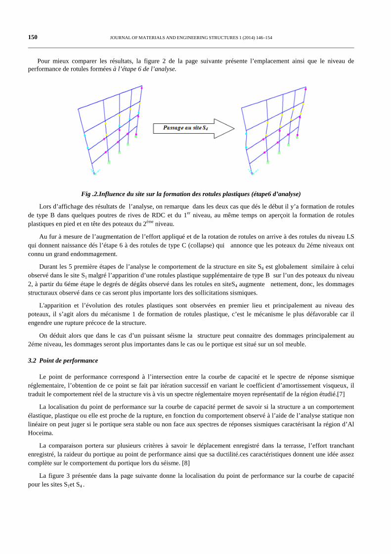
150 JOURNAL OF MATERIALS AND ENGINEERING STRUCTURES 1 (2014) 146–154
Pour mieux comparer les résultats, la figure 2 de la page suivante présente l’emplacement ainsi que le niveau de performance de rotules formées à l’étape 6 de l’analyse.
Fig .2.Influence du site sur la formation des rotules plastiques (étape6 d’analyse)
Lors d’affichage des résultats de l’analyse, on remarque dans les deux cas que dés le début il y’a formation de rotules de type B dans quelques poutres de rives de RDC et du 1er niveau, au même temps on aperçoit la formation de rotules plastiques en pied et en tête des poteaux du 2éme niveau.
Au fur à mesure de l’augmentation de l’effort appliqué et de la rotation de rotules on arrive à des rotules du niveau LS qui donnent naissance dés l’étape 6 à des rotules de type C (collapse) qui annonce que les poteaux du 2éme niveaux ont connu un grand endommagement.
Durant les 5 première étapes de l’analyse le comportement de la structure en site S4 est globalement similaire à celui observé dans le site S1 malgré l’apparition d’une rotules plastique supplémentaire de type B sur l’un des poteaux du niveau 2, à partir du 6éme étape le degrés de dégâts observé dans les rotules en siteS4 augmente nettement, donc, les dommages structuraux observé dans ce cas seront plus importante lors des sollicitations sismiques.
L'apparition et l’évolution des rotules plastiques sont observées en premier lieu et principalement au niveau des poteaux, il s’agit alors du mécanisme 1 de formation de rotules plastique, c’est le mécanisme le plus défavorable car il engendre une rupture précoce de la structure.
On déduit alors que dans le cas d’un puissant séisme la structure peut connaitre des dommages principalement au 2éme niveau, les dommages seront plus importantes dans le cas ou le portique est situé sur un sol meuble.
3.2 Point de performance
Le point de performance correspond à l’intersection entre la courbe de capacité et le spectre de réponse sismique réglementaire, l’obtention de ce point se fait par itération successif en variant le coefficient d’amortissement visqueux, il traduit le comportement réel de la structure vis à vis un spectre réglementaire moyen représentatif de la région étudié.[7]
La localisation du point de performance sur la courbe de capacité permet de savoir si la structure a un comportement élastique, plastique ou elle est proche de la rupture, en fonction du comportement observé à l’aide de l’analyse statique non linéaire on peut juger si le portique sera stable ou non face aux spectres de réponses sismiques caractérisant la région d’Al Hoceima.
La comparaison portera sur plusieurs critères à savoir le déplacement enregistré dans la terrasse, l’effort tranchant enregistré, la raideur du portique au point de performance ainsi que sa ductilité.ces caractéristiques donnent une idée assez complète sur le comportement du portique lors du séisme. [8]
La figure 3 présentée dans la page suivante donne la localisation du point de performance sur la courbe de capacité pour les sites S1et S4 .

JOURNAL OF MATERIALS AND ENGINEERING STRUCTURES 1 (2014) 146–154 151
Fig.3 Influence du site sur le point de performance
Le tableau 6 ci-dessous résume les caractéristiques du point de performance dans le cas ou le portique est construit sur un sol classé site S1 et celui d’un sol classé site S4 :
Tableau 6. Influence du site sur le point de performance.
Caractéristique du point de performance en site S1 Caractéristique du point de performance en site S4
Effort tranchant à la base (KN) 68,165 Effort tranchant à la base (KN) 95,126
Déplacement de la terrasse (cm) 1,9 Déplacement de la terrasse (cm) 3,5
Raideur au point de performance (KN/cm)
35,876 Raideur au point de performance
(KN/cm)
27,178
Accélération spectrale 0,448 Accélération spectrale 0,667
Déplacement spectral (cm) 1,4 Déplacement spectral (cm) 2,7
Ductilité 1,077 Ductilité 1,581
Pour le cas du sol représentant le site S1, la figure qui localise le point de performance permet de dire que le portique étudié à globalement un comportement élastique, la ductilité qui traduit la capacité de la structure à dissiper l’énergie en rentrant dans des déformations plastique montre avec sa valeur 1,077>1 que le portique commence à rentrer dans le domaine plastique et les rotules vont commencer à se former principalement dans les poutres de RDC et dans les poteaux du 2éme niveau.
Les valeurs de l’effort tranchant à la base et le déplacement de la terrasse au point de performance indiquent en se basant sur les tableaux données par le logiciel SAP2000 lors d’affichage des résultats de l’analyse que le comportement de la structure est donné par la 2éme étape de l’analyse, on peut alors commencer à avoir des fissures dans les poteaux du 2éme niveau ainsi que sur quelques poutres, la classification du EMS98 permet de dire que le portique a subit des dégâts de degré 2.
Etant donné que la structure est sans conception parasismique elle est de classe de vulnérabilité ‘C’ et sachant que les spécialistes ont attribué au séisme d’Al Hoceima2004 une intensité VIII, on peut dire que la classification des dommages de structures en terme de vulnérabilité donné par l’EMS98 qui attribut généralement pour ce type de structures des dégâts de degré 2correspond aux résultats trouvés par l’analyse statique non linéaire.
Pour le cas du sol représentant le site S4 La position du point de performance sur la figure permet de dire que le portique étudié à globalement un comportement plastique, la ductilité montre avec sa valeur 1,581>1 que la plastification

152 JOURNAL OF MATERIALS AND ENGINEERING STRUCTURES 1 (2014) 146–154
des rotules dans la structure est avancée, les valeurs de l’effort tranchant 95,126 KN et du déplacement du toit 3,5 cm dépassent largement les valeurs enregistré pour le même portique en site S1, cette différence se traduit par le passage d’une raideur de 27,178KN/m en site S4 à une raideur de 35,876 KN/m en site S1 ce qui correspond à une augmentation de 32% dans la résistance du portique en passant du site S4 au site S1.
Les valeurs de l’effort tranchant à la base et le déplacement de la terrasse au point de performance du site S4 indiquent que le comportement de la structure est donné par la 6éme étape de l’analyse (Fig1.), on va observer des fissures dans les éléments structuraux de tous les niveaux, les poteaux du 2éme niveau peuvent connaitre même un basculement, le degré de dégâts est alors 3.
Le degré de dégâts 3 est fournit rarement par l’EMS98 pour les structures de classe de vulnérabilité C subissant des séismes d’intensité VIII, le cas d’un portique de classe de vulnérabilité C en site défavorable en particulier donne ce résultat.
Le séisme d’AL Hoceima 2004 a causé la mort de 629 personnes suite à l’effondrement de leurs bâtiments, la majorité de structures qui ont connu la ruine sont de type maçonnerie (à Ait Kamra), les constructions en béton armé existantes étaient tous sans conception parasismique, cependant il y’a des constructions qui ont connu d’importantes dégâts voir la ruine et d’autres qui ont connu des dégâts légers ceci peut s’expliquer par :[9]
L’influence du site : on a vu que les bâtiments en béton armé construits sur des sols meubles sont plus vulnérables aux séismes que ceux construits sur des sols rocheux ou ferme, ces derniers vont connaitre généralement de faible dégâts réparable et qui n’influence pas sur la stabilité structurelle en assurant le sauvegarde de vie.
La qualité d’exécution : les dégâts excessifs remarqués sur certaines structures au même temps que des structures voisines n’ont pas été très touchées sont généralement lié à des problèmes de suivi et de non respect du plan de béton armé.
3.3 Vérification de la fonctionnalité du portique
Le tableau ci-dessous résume les résultats de déplacements et déplacements inter étage obtenus de lors de l’analyse statique non linéaire, ces résultats correspondent aux déplacements maximum des nœuds du portique prés du point de performance
On désigne par :
D : Le déplacement de l’étage
∆𝐷𝐷 : Le déplacement inter-étages
Tableau 7. Déplacement inter étages du portique de rive pour les sites S1 et S4
Portique de rive site S1 Portique de rive site S4
Niveau D (cm) ∆𝑫𝑫 (mm) Niveau D(cm) ∆𝑫𝑫(mm)
RDC 0,42 4,2 RDC 0,57 5,7
Niveau 1 0,88 4,6 Niveau 1 1,22 6,5
Niveau2 1,58 7 Niveau2 3,05 18,3
Niveau3 1,95 3,7 Niveau3 3,55 5
Le déplacement limite inter-étage qui ne doit pas être dépassé pour assurer la fonctionnalité de la structure en terme de déplacement est selon RPS2000 :
∆Dlim= 0,01h/K (1)
h : représente la hauteur de l’étage ; dans notre cas h = 3m.
K : Le facteur de comportement : dans notre cas K=2

JOURNAL OF MATERIALS AND ENGINEERING STRUCTURES 1 (2014) 146–154 153
Alors :
a ∆Dlim= 0,005h = 0,015m = 15mm (2)
h : représente la hauteur de l’étage ; dans notre cas h = 3m
K : facteur de comportement : dans notre cas K=2
Pour le portique en site S1 la fonctionnalité est assurée car le déplacement maximal inter-étage enregistré au niveau 2 est inférieur au déplacement limite imposé par la réglementation :
7mm<15mm
Pour le portique de rive en site S4 la fonctionnalité n’est pas assurée car le déplacement maximal inter-étage enregistré au niveau 2 est supérieur au déplacement limite imposé par la réglementation :
18,3mm>15mm
Le changement de site peut influencer d’une manière très importante sur la fonctionnalité de la structure, la nature de sol influence sur le comportement inter-étage.
Pour mieux comparer les résultats de déplacements inter-étages on regroupe les déplacements inter-étage dans un même graphe comme le montre la figure ci-dessous :
Fig. 4. Influence du site sur le déplacement inter-étages.
On remarque que à part le niveau 2 le déplacement inter-étage en site S4 est légèrement plus important que celui en site S1, cependant au niveau 2 l’augmentation du déplacement inter-étage au site S4 par rapport au site S1 a atteint 226% ce qui a compromis la fonctionnalité du portique.
Le portique étudié appartient à une structure dimensionnée sans conception parasismique, le niveau 2 avait pour section de poteaux 20 x 20 ; bien que cette section est suffisante pour reprendre les efforts de compression, elle ne supporte pas les charges sismiques qui engendrent une flexion composée. L’exigence du RPS2000 d’une section minimale de 25x25 se trouve ainsi justifiée car on a vu que les grands dommages en matière de rotules et en déplacement inter-étages sont enregistrés au niveau 2.
4 Conclusion
L’analyse statique non linéaire a permis de montrer l’influence du site sur les dégâts observés lors de séismes, les structures sans conception parasismiques nécessitent généralement des renforcements pour pourvoir résister aux sollicitations sismiques que la région d’Al Hoceima peut connaitre, ces renforcement vont assurer plus de rigidité et de ductilité à la structure
154 JOURNAL OF MATERIALS AND ENGINEERING STRUCTURES 1 (2014) 146–154
REFERENCES
[1]- ATC, Seismic Evaluation and Retrofit of Concrete Buildings, Vol. 1, ATC-40 Report, Applied Technology Council, Redwood City, USA, 1996.
[2]- Règlement de construction parasismique RPS 2000, Ministère de l’ATUHE, Secrétariat d’État de l’Habitat, Royaume du Maroc, 2011.
[3]- P. Fajfar, Capacity spectrum method based on inelastic demand spectra. Earthquake Eng. Struct. 28(9)(1999) 979-993.
[4]- L’échelle Macrosismique Européenne, Cahier du Centre Européen de Géodynamique et de Séismologie. Ed. Conseil de l’Europe, Vol. 19, 1998
[5]- SAP2000, Integrated Finite Element Analysis, SAP2000 Web tutorial 1: Detailed tutorial including pushover analysis. Computer and structures Inc, Berkeley, California, 1998.
[6]- SAP2000, Integrated Finite Element Analysis, SAP2000 Web tutorial 2: Quick pushover analysis tutorial. Computer and structures Inc, Berkeley, California, 1998.
[7]- Federal Emergency Management Agency, NEHRP recommended Provisions for Seismic Regulations for New Buildings and Other Structures: FEMA273, 2003.
[8]- R. Bento, S. Falcao, F. Rodrigues, Nonlinear Static Procedures in Performance Based Seismic Design. In: Proceedings of the 13th world conference on earthquake engineering, Vancouver, Canada,
[9]- M. Saiidi, MA. Sozen, Simple Nonlinear response of R/C Structures. J. Struct. Div-ASCE. 107(5)(1981) 937-953.

JOURNAL OF MATERIALS AND ENGINEERING STRUCTURES 1 (2014) 155–168
155
Research Paper
Comportement d’un matériau sablo-graveleux sur chemin cyclique Behavior of a gravel-sand material on cyclic way
Hocine Bendadouche*,a, Khemmoudj Kaddour b, Merabet Smail a a Université de Béjaïa, Faculté de Technologie, Béjaïa, Algérie b Université de Béjaïa, Faculté des sciences naturelles, Béjaïa, Algérie
A R T I C L E I N F O
Historique de l’article :
Recu : 25 mai 2014
Révisé : 27 octobre 2014
Accépté : 8 novembre 2014
R E S U M E
Cet article présente les résultats des essais triaxiaux cycliques pour étudier le potentiel de liquéfaction d’un matériau sablo-graveleux. De nombreux articles sont consacrés aux essais sur le sable de laboratoire type Hostun notamment pour l’étude de la liquéfaction ou sur des argiles reconstituées mais peu d’essais sont effectués sur un matériau naturel. La rareté des essais cycliques sur les matériaux naturels notamment grossiers, montre la difficulté d’évaluer le risque sismique. Devant ces difficultés, l’utilisation des essais comme le CPT permet une approche différente mais très pratique. L’ensemble des résultats montre une tendance à la liquéfaction relativement importante du matériau, même dans des conditions de sollicitation modérées (qc/2σ’3 = 0.2). Cette tendance s’accroît très fortement quand le taux de sollicitation cyclique atteint 0.3. L’essai au CPT montre également une grande tendance à la liquéfaction avec un coefficient de sécurité largement inférieure à 1.
A B S T R A C T
This article has the results of the cyclic triaxial compression tests to study the potential of liquefaction of a gravel-sand material. The last part is devoted to the not drained cyclic tests and their analyses. Many articles are devoted to the tests on the standard sand of laboratory Hostun in particular for the study of liquefaction or on reconstituted clays but few tests are carried out on a natural material. The scarcity of cyclic tests on such rough natural materials shows the difficulty of assessing the seismic risk. Faced with these difficulties, the use of tests such as the CPT provides a different but very practical approach. The overall results show a trend of relatively high liquefaction of the material, even under conditions of moderate stress (qc / 2σ'3 = 0.2) . This trend is growing very strongly when the rate of cyclic loading reached 0.3. The CPT test also shows a great tendency to liquefaction with a safety factor of well below 1.
Mots clés:
Liquéfaction
Chargement cyclique
Pression intersticielle
C.P.T.
Keywords :
Liquefaction
Cyclic loading
Pore water pressure
C.P.T.
* Corresponding author. Tel.: 07 73 47 04 67. E-mail address: [email protected] e-ISSN: 2170-127X, © Mouloud Mammeri University of Tizi-Ouzou, Algeria

156 JOURNAL OF MATERIALS AND ENGINEERING STRUCTURES 1 (2014) 155–168
1 Introduction
Les digues sont de fait des infrastructures d'une importance capitale pour l'économie d’où la nécessite de considérer très sérieusement les risques de liquéfaction sous l’action des séismes.
Bambara et al. [1] d’Aix-en-Provence (France), ont proposé la première caractérisation du risque de liquéfaction sous sollicitation sismique d’ouvrages hydraulique en remblai existants ou projetés en basse vallée du Rhône.
L’étude de la sensibilité du site à la liquéfaction est donc une nécessité vitale. Ce phénomène a pour conséquence la perte complète de la résistance au cisaillement et la ruine de l’ouvrage. C’est dans ce cadre que la digue rive gauche du Canal d’Alsace au niveau du bief de KEMBS a fait l’objet d’une étude de réévaluation sismique pour identifier les risques de liquéfaction du site à partir des essais de laboratoires et des essais in situ basés sur le C.P.T.
Les essais de laboratoire ont permis de connaître le comportement du sol de connaître la réponse cyclique aux petites et moyennes déformations, d’identifier le risque de liquéfaction, de définir le comportement résiduel post-sismique. Ces essais de laboratoire nécessitent des prélèvements d'échantillons intacts souvent difficiles dans les couches sablo-graveleux. Les essais triaxiaux cycliques permettant d'établir une courbe de résistance à la liquéfaction nécessitent des échantillons représentatifs et sont coûteux. Une alternative est alors l'étude du risque de liquéfaction à partir des essais in situ à la suite des travaux de Seed et Idriss [2]. Initialement développée à partir du S.P.T. (Standard pénétration test), cette méthode a été étendue à l'essai de pénétration statique (CPT, Cône Pénétration Test).
L’évaluation de la stabilité sismique des digues est une tache longue qui nécessite une méthodologie progressive. Le problème principal est la détection de zones à la liquéfaction pourrait se développer. Le pénétromètre est l’outil adapté à cette situation. Les essais triaxiaux de liquéfaction en sont le complément indispensable. Ces derniers permettent d’obtenir les propriétés de résistance, les propriétés de déformations et enfin, le potentiel de liquéfaction du matériau. L’essai cyclique au triaxial est le plus représenté des essais de cisaillement cycliques, il permet de créer en laboratoire toutes les conditions de terrain souhaitées.
1.1 Problématique
Le but de cet étude est la réévaluation sismique de la digue rive gauche du Canal d’Alsace, au niveau du bief de Kembs, EDF a fait procéder à des reconnaissances géotechniques et à la réalisation d’un sondage carotté de 13m au PK Rhin 177,2.
Une grande partie de cet article est consacré aux conditions expérimentales notamment à l’identification du matériau, la fabrication des échantillons, leur saturation.
Le prélèvement intact des matériaux sableux est souvent impossible à effectuer à cause de l’absence de cohésion dans ce type de sol. La représentativité du matériau employé pose toujours problème. Devant ces difficultés, l’utilisation des essais in situ permet une approche différente mais très pratique.
1.2 La liquéfaction
Le phénomène de densification des sables denses peut être mis en évidence d'une façon simple par chargement cyclique avec dépassement de seuil des caractéristiques en compression et en extension triaxiale. Cette sollicitation à grande amplitude bénéficie d'un effacement de l'écrouissage lors de la phase dilatante qui déchevêtre la structure granulaire du squelette solide. A chaque recharge, le mécanisme de serrage engendre de nouvelles déformations volumétriques irréversibles et se répète pour un nouveau matériau devenu chaque fois plus dense. L'instabilité de liquéfaction est correctement interprétée par le concept d'état caractéristique. Dès que la contrainte effective atteint le seuil caractéristique en compression comme en extension, le point figuratif remonte la ligne caractéristique. La déformation devient de plus en plus grande lors de la décharge entraînant un accroissement sensible de la pression interstitielle qui s'accumule au cours des cycles jusqu'à la ruine de l'échantillon.
Le phénomène de liquéfaction totale n'est possible que si le chargement est alterné autour de l'état q=0. Vaid et Chern [3] ont montré dans la figure 1, le comportement du sable d'Ottawa soumis à des chargements cycliques alternés. Deux densités relatives ont été utilisées : Dr=0.33 pour les sables lâches et Dr=0.71 pour le sable dense.

JOURNAL OF MATERIALS AND ENGINEERING STRUCTURES 1 (2014) 155–168 157
Dans le plan (q, p') qui représente le cheminement cyclique des contrainte, on a remarqué que dés que le chemin de contrainte effective atteint le seuil caractéristique en compression comme en extension, il remonte la ligne caractéristique.
Fig. 1 Chemin de contrainte effectif d’un échantillon de sable. Vaid et Chern [3]
1.3 Paramètres influençant le phénomène de liquéfaction
D’après Seed et Lee [4], il a été reconnu que la densité relative et la contrainte de consolidation étaient les principaux facteurs qui pouvaient influencer les caractéristiques de liquéfaction cyclique d’un sol.
Le nombre de cycles nécessaires à la liquéfaction augmente avec :
- l’augmentation de la pression de confinement, de la densité relative et du déviateur cyclique (résultats de Vilela [5] sur le sable de Grandville).
Les autres facteurs qui peuvent influencer la liquéfaction sont :
- Le coefficient de poussée des terres au repos Ko - L’histoire des déformations - La granulométrie - La qualité des échantillons
1.4 Situation géographique Kembs est un arrondissement de Mulhouse (Haut Rhin Alsace). Il est situé (Fig.2) à la longitude 07° 30' 16" Est et à
latitude 47° 41' 23" Nord. Son altitude moyenne est de : 241 m.
Fig. 2. Carte de situation du département de Haut et Bas Rhin
1.5 Contexte sismique de Kembs
La région de Haut Rhin (Kembs) est située dans la zone II (sismicité moyenne) mais c’est la plus élevée de la France métropolitaine. Une secousse d'intensité supérieure à IX a été observée historiquement. Les périodes de retour d'une secousse d'intensité supérieure ou égale à VIII et d'une secousse d'intensité supérieure ou égale à VII sont respectivement
Kembs
σ'1+σ'3)/2, kg/cm2
σ'1-
σ'3)
/2, k
g/cm
2
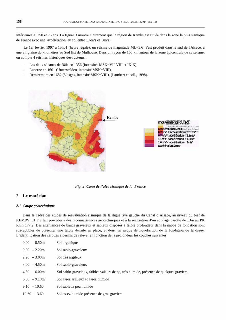
158 JOURNAL OF MATERIALS AND ENGINEERING STRUCTURES 1 (2014) 155–168
inférieures à 250 et 75 ans. La figure 3 montre clairement que la région de Kembs est située dans la zone la plus sismique de France avec une accélération au sol entre 1.6m/s et 3m/s.
Le 1er février 1997 à 15h01 (heure légale), un séisme de magnitude ML=3.6 s'est produit dans le sud de l'Alsace, à une vingtaine de kilomètres au Sud Est de Mulhouse. Dans un rayon de 100 km autour de la zone épicentrale de ce séisme, on compte 4 séismes historiques destructeurs :
- Les deux séismes de Bâle en 1356 (intensités MSK=VII-VIII et IX-X), - Lucerne en 1601 (Unterwalden, intensité MSK=VIII), - Remiremont en 1682 (Vosges, intensité MSK=VIII), (Lambert et coll., 1998).
Fig. 3 Carte de l’aléa sismique de la France
2 Le matériau
2.1 Coupe géotechnique
Dans le cadre des études de réévaluation sismique de la digue rive gauche du Canal d’Alsace, au niveau du bief de KEMBS, EDF a fait procéder à des reconnaissances géotechniques et à la réalisation d’un sondage carotté de 13m au PK Rhin 177,2. Des alternances de bancs graveleux et sableux disposés à faible profondeur dans la nappe de fondation sont susceptibles de présenter une faible densité en place, et donc un risque de liquéfaction de la fondation de la digue. L’identification des carottes a permis de relever en fonction de la profondeur les couches suivantes :
0.00 – 0.50m Sol organique
0.50 – 2.20m Sol sablo-graveleux
2.20 – 3.00m Sol très argileux
3.00 – 4.50m Sol sablo-graveleux
4.50 – 6.00m Sol sablo-graveleux, faibles valeurs de qc, très humide, présence de quelques graviers.
6.00 – 9.10m Sol assez argileux et assez humide
9.10 – 10.60 Sol sableux peu humide
10.60 – 13.60 Sol assez humide présence de gros graviers
mouvements du solaccélération<0.7m/s²0.7m/s² ≤ accélération < 1.1m/s²0.7m/s² < accélération < 1.1m/s²1.1m/s² < accélération < 1.6m/s²1.6m/s² < accélération < 3m/s²accélération≥3m/s²
accélération au sol entre 1.6m/s et 3m/s.
Kembs
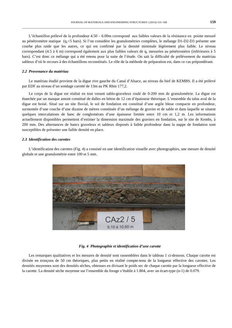
JOURNAL OF MATERIALS AND ENGINEERING STRUCTURES 1 (2014) 155–168 159
L’échantillon prélevé de la profondeur 4.50 – 6.00m correspond aux faibles valeurs de la résistance en pointe mesuré au pénétromètre statique (qc<5 bars). Si l’on considère les granulométries complètes, le mélange D1-D2-D3 présente une courbe plus raide que les autres, ce qui est confirmé par la densité minimale légèrement plus faible. Le niveau correspondant (4.5 à 6 m) correspond également aux plus faibles valeurs de qc mesurées au pénétromètre (inférieures à 5 bars). C’est donc ce mélange qui a été retenu pour la suite de l’étude. On sait la difficulté de prélèvement du matériau sableux d’où le recours à des échantillons reconstitués. Le rôle de la méthode de préparation est, dans ce cas prépondérant.
2.2 Provenance du matériau
Le matériau étudié provient de la digue rive gauche du Canal d’Alsace, au niveau du bief de KEMBS. Il a été prélevé par EDF au niveau d’un sondage carotté de 13m au PK Rhin 177,2.
Le corps de la digue est réalisé en tout venant sablo-graveleux roulé de 0-200 mm de granulométrie. La digue est étanchée par un masque amont constitué de dalles en béton de 12 cm d’épaisseur théorique. L’ensemble du talus aval de la digue est boisé. Situé sur un site fluvial, le sol de fondation est constitué d’une argile bleue compacte en profondeur, surmontée d’une couche d’une dizaine de mètres constituée d’un mélange de gravier et de sable et dans laquelle se situent quelques intercalations de banc de conglomérats d’une épaisseur limitée entre 10 cm et 1,2 m. Les informations actuellement disponibles permettent d’estimer la dimension maximale des graviers en fondation, sur le site de Kembs, à 200 mm. Des alternances de bancs graveleux et sableux disposés à faible profondeur dans la nappe de fondation sont susceptibles de présenter une faible densité en place.
2.3 Identification des carottes
L’identification des carottes (Fig. 4) a consisté en une identification visuelle avec photographies, une mesure de densité globale et une granulométrie entre 100 et 5 mm.
Fig. 4 Photographie et identification d’une carotte
Les remarques qualitatives et les mesures de densité sont rassemblées dans le tableau 1 ci-dessous. Chaque carotte est divisée en tronçons de 50 cm théoriques, plus petits en réalité compte-tenu de la longueur effective des carottes. Les densités moyennes sont des densités sèches, obtenues en divisant le poids sec de chaque carotte par la longueur effective de la carotte. La densité sèche moyenne sur l’ensemble du forage s’établit à 1.804, avec un écart-type (n-1) de 0.079.

160 JOURNAL OF MATERIALS AND ENGINEERING STRUCTURES 1 (2014) 155–168
Tableau 1. Identification de la carotte : Digue de Kembs – PK 177.200 (Rive Gauche)
Profondeur Description
A1
0 -1.55 m
Haut
DIGUE
Matière organique Longueur : 1.27 m Densité moyenne de la carotte = 1.71
A2 Milieu
A3 Bas
B1 1.55 –3 m
Haut Longueur : 0.87 m Densité moyenne de la carotte = 1.74 B2 Bas Zone très argileuse
C1
3.0 –4.5 m
Haut Longueur : 1.18 m Densité moyenne de la carotte = 1.74
C2 Milieu
C3 Bas
D1
4.5 –6 m
Haut Zone de faibles qc, très humide, quelques gros graviers
Longueur : 1.31 m Densité moyenne de la carotte = 1.81
D2 Milieu
D3 Bas
E1
6.0 –7.5 m
Haut
Zone assez humide, assez argileuse
Longueur : 1.29 m Densité moyenne de la carotte = 1.91
E2 Milieu
E3 Bas
F1
7.5 –9.1 m
Haut Longueur : 1.44 m Densité moyenne de la carotte = 1.78
F2 Milieu
F3 Bas
FONDATION
moins argileux
G1
9.1 –10.6 m
Haut
Zone peu argileuse Longueur : 1.44 m Densité moyenne de la carotte = 1.95
G2 Milieu
G3 Bas
H1
10.6 –12.1 m
Haut
Zone très sableuse, peu humide
Longueur : 1.47 m Densité moyenne de la carotte = 1.80
H2 Milieu
H3 Bas
I1
12.1 –13.6 m
Haut Longueur : 1.18 m Densité moyenne de la carotte = 1.80
I2 Milieu Présence de gros graviers, assez humide I3 Bas
L’identification des carottes a consisté en une identification visuelle avec photographies, une mesure de densité globale
et une granulométrie entre 100 et 5 mm.

JOURNAL OF MATERIALS AND ENGINEERING STRUCTURES 1 (2014) 155–168 161
2.4 Granulométrie
Les mesures granulométriques ont été faites à sec, en faisant passer les matériaux à travers les tamis de 100, 63, 25, 12.5, 10, 5 mm par vibration et pinceau. Les résultats sont représentés dans la figure 5.
10 100 1000 10000 100000Diamètre du tamis (µm)
0
10
20
30
40
50
60
70
80
90
100Pa
ssan
t (%
)
MélangeD1-D2-D3
Fig. 5 Granulométrie du mélange utilisé dans les essais
3 Méthodes
- Fabrication et mise en place des échantillons ; détermination des caractéristiques initiales
- Pré-saturation par circulation sous faible gradient et saturation par contre-pression,
- Mesure du paramètre de Skempton B
- Consolidation isotrope ou anisotrope,
- Ecrasement monotone
3.1 Fabrication et mise en place des échantillons ; détermination des caractéristiques initiales
Le matériau est mis en place en 1 couche de 4 cm et 6 couches de 3 cm d’épaisseur, à une teneur en eau de 4 % pour les échantillons de faible densité, sec pour les échantillons de forte densité, à l’intérieur de la membrane en latex tendue sur un moule rigide (Fig.6). On détermine par avance la masse sèche de matériau à mettre en place dans chaque couche en fonction des caractéristiques choisies. Le matériau est mis en place avec précaution à l’intérieur du moule, puis plus ou moins compacté (par compression ou petits chocs) jusqu’à ce que l’épaisseur de la couche corresponde à la masse sèche de matériau et à la densité choisie. Dans le moule, les dimensions de l’échantillon sont de 102 mm x 220 mm.
Le moule repose sur une plaque d’anti-frettage posée sur la base de la cellule, un vide est appliqué entre le moule et la membrane pour la maintenir tendue. La plaque d’antifrettage consiste en une plaque lisse de diamètre (12 cm) supérieur à celui de la base, enduite de graisse, sur laquelle glissent des secteurs de membrane au contact de l’échantillon. Une fois le moule rempli, on met en place à la partie supérieure la seconde plaque d’antifrettage et la tête de l’échantillon. Le moule en deux parties est alors retiré avec précaution et on mesure les dimensions extérieures de l’échantillon au moyen d’un pied à coulisse (2 mesures de diamètre à 3 niveaux et 4 mesures de hauteur). On applique éventuellement un vide léger à l’intérieur de l’échantillon pour le maintenir stable jusqu’à application de la contrainte de confinement initiale.
On met ensuite en place l’enveloppe extérieure de la cellule que l’on remplit d’eau, en évitant les surpressions. On applique alors une pression de confinement de 30 kPa et l’on fait entrer l’air dans l’échantillon (suppression du vide).

162 JOURNAL OF MATERIALS AND ENGINEERING STRUCTURES 1 (2014) 155–168
Fig. 6. Fabrication des échantillons
4 Résultats et discussions
Les résultats de tous les essais ont été regroupés sur le tableau 2 où sont indiquées les principales conditions de chaque essai et le nombre de cycles ayant conduit à la liquéfaction, celle-ci étant toujours définie par la condition de déformation maximale supérieure à 5% entre le maximum et le minimum, plutôt que par la condition de contrainte effective de confinement nulle que l’on observe parfois mais pas systématiquement.
Nous avons illustré sur les figures 7 et 8 les deux comportements extrêmes observés :
celui d’un échantillon très dense (220 LIQ23) soumis à un chargement déviatorique moyen (qc/2σ’3 = 0.2),
celui d’un échantillon peu dense (146 LIQ2) soumis à un chargement déviatorique fort (qc/2σ’3 = 0.3)
ableau 2. Conditions de liquéfaction des échantillons
Essais Contrainte de consolidation
kPa qc /2 σ’3
DR après saturation
%
DR après consolidation
%
Nombre de cycles jusqu’à liquéfaction
ε1 > 5%
146LIQ10 200 0.15 43 57 10
146LIQ9 400 0.15 57 76 23
146LIQ8 50 0.20 49 54 3-4
146LIQ1 200 0.20 40 56 8-9
146LIQ21 400 0.20 49 66 4
146LIQ20 σ’3 = 200 σ’1 = 400
0.20 46 59 5-6
146LIQ2 200 0.30 - 58 1
189LIQ12 200 0.20 54 69 15
189LIQ22 σ’3 = 200 σ’1 = 400
0.20 50 68 > 30
200LIQ11 200 0.20 64 79 > 30
220LIQ23 200 0.20 87 89 > 30
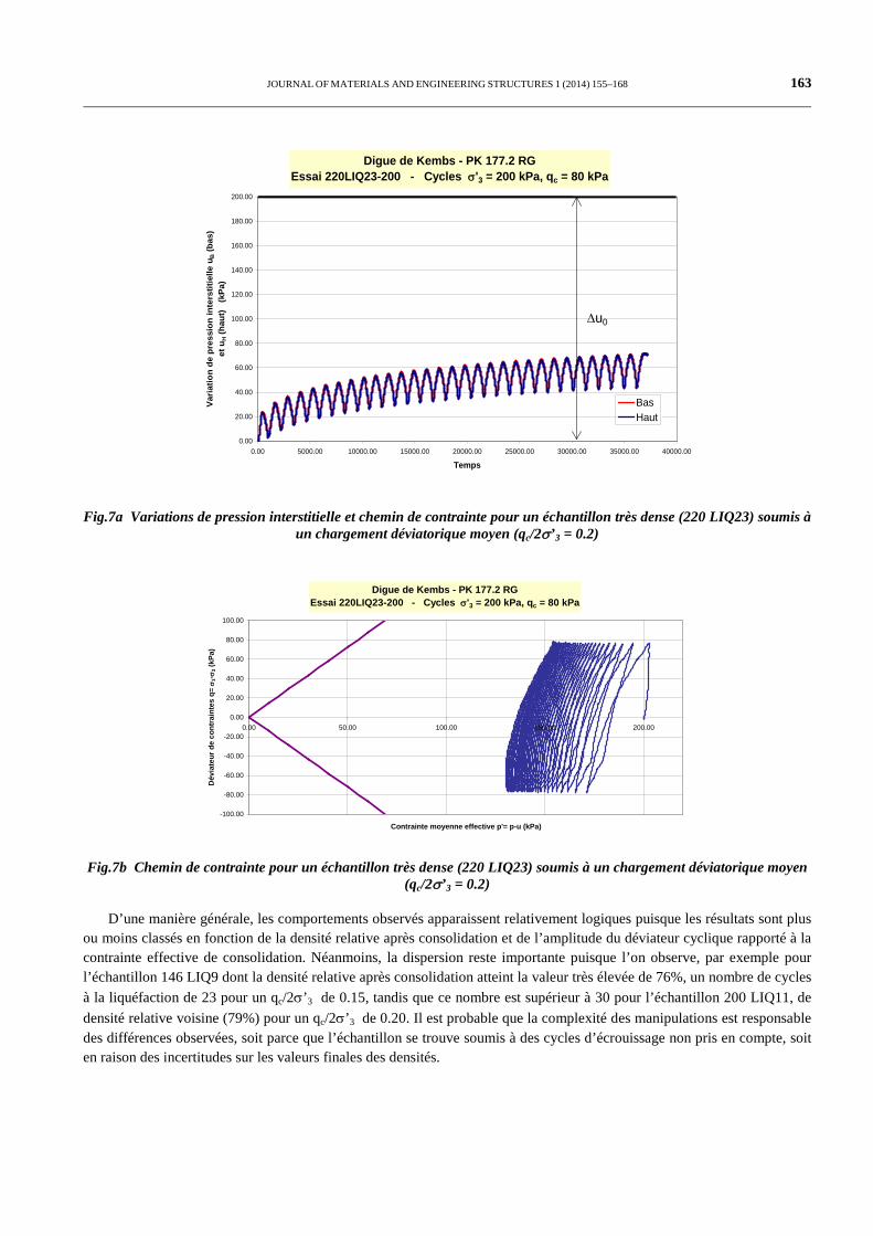
JOURNAL OF MATERIALS AND ENGINEERING STRUCTURES 1 (2014) 155–168 163
Fig.7a Variations de pression interstitielle et chemin de contrainte pour un échantillon très dense (220 LIQ23) soumis à un chargement déviatorique moyen (qc/2σ’3 = 0.2)
Fig.7b Chemin de contrainte pour un échantillon très dense (220 LIQ23) soumis à un chargement déviatorique moyen (qc/2σ’3 = 0.2)
D’une manière générale, les comportements observés apparaissent relativement logiques puisque les résultats sont plus ou moins classés en fonction de la densité relative après consolidation et de l’amplitude du déviateur cyclique rapporté à la contrainte effective de consolidation. Néanmoins, la dispersion reste importante puisque l’on observe, par exemple pour l’échantillon 146 LIQ9 dont la densité relative après consolidation atteint la valeur très élevée de 76%, un nombre de cycles à la liquéfaction de 23 pour un qc/2σ’3 de 0.15, tandis que ce nombre est supérieur à 30 pour l’échantillon 200 LIQ11, de densité relative voisine (79%) pour un qc/2σ’3 de 0.20. Il est probable que la complexité des manipulations est responsable des différences observées, soit parce que l’échantillon se trouve soumis à des cycles d’écrouissage non pris en compte, soit en raison des incertitudes sur les valeurs finales des densités.
Digue de Kembs - PK 177.2 RGEssai 220LIQ23-200 - Cycles σ'3 = 200 kPa, qc = 80 kPa
-100.00
-80.00
-60.00
-40.00
-20.00
0.00
20.00
40.00
60.00
80.00
100.00
0.00 50.00 100.00 150.00 200.00
Contrainte moyenne effective p'= p-u (kPa)
Dév
iate
ur d
e co
ntra
inte
s q=
σ1-
σ 3 (k
Pa)
Digue de Kembs - PK 177.2 RGEssai 220LIQ23-200 - Cycles σ'3 = 200 kPa, qc = 80 kPa
0.00
20.00
40.00
60.00
80.00
100.00
120.00
140.00
160.00
180.00
200.00
0.00 5000.00 10000.00 15000.00 20000.00 25000.00 30000.00 35000.00 40000.00
Temps
Varia
tion
de p
ress
ion
inte
rstit
ielle
uB (b
as)
et u
H (h
aut)
(kP
a)
BasHaut
∆u0

164 JOURNAL OF MATERIALS AND ENGINEERING STRUCTURES 1 (2014) 155–168
Fig.8a Variations de pression interstitielle et chemin de contrainte pour un échantillon peu dense (146 LIQ2) soumis à un chargement déviatorique fort (qc/2σ’3 = 0.3)
Fig.8b Chemin de contrainte pour un échantillon peu dense (146 LIQ2) soumis à un chargement déviatorique fort (qc/2σ’3 = 0.3)
Les différents résultats disponibles ont été rassemblés sur la figure 9.
Digue de Kembs - PK 177.2 RGEssai 146LIQ2-200 - Cycles σ'3 = 200 kPa, qc = 120 kPa
-150.00
-100.00
-50.00
0.00
50.00
100.00
150.00
0.00 20.00 40.00 60.00 80.00 100.00 120.00 140.00 160.00 180.00 200.00
Contrainte moyenne effective p'= p-u (kPa)
Dév
iate
ur d
e co
ntra
inte
s q=
σ1-
σ3
(kP
a)
Digue de Kembs - PK 177.2 RGEssai 146LIQ2-200 - Cycles σ'3 = 200 kPa, qc = 120 kPa
0.00
20.00
40.00
60.00
80.00
100.00
120.00
140.00
160.00
180.00
200.00
0.00 500.00 1000.00 1500.00 2000.00 2500.00 3000.00 3500.00 4000.00 4500.00 5000.00
Temps
Var
iatio
n de
pre
ssio
n in
ters
titie
lle u
B (b
as)
et u
H (h
aut)
(k
Pa)
BasHaut
∆u0

JOURNAL OF MATERIALS AND ENGINEERING STRUCTURES 1 (2014) 155–168 165
Fig.9 Nombre de cycles conduisant à la liquéfaction en fonction du taux de sollicitation cyclique pour les différents échantillons consolidés isotropiquement.
Quatre essais cycliques ont été suivis par l’application d’un cycle de compression-extension : les essais 146 LIQ20, 189 LIQ22, 200 LIQ11 et 220 LIQ23. Les échantillons présentent des densités relatives en fin de consolidation comprises entre 68 et 89%. Dans certains cas, des problèmes de pilotage de la presse (instabilités lors du passage du contrôle en force au contrôle en déplacement) n’ont pas permis d’aller jusqu’au bout des essais.
Les résultats sont présentés sur la figure 10 dans le plan de la variation de pression interstitielle à la base en fonction de la déformation axiale et dans le plan du chemin de contraintes. Dans le premier cas, on note toujours une augmentation initiale de pression suivie d’une diminution lors du chargement, qui traduise un comportement surconsolidé du matériau. Lors du déchargement, le phénomène s’inverse et la pression commence par augmenter avant de diminuer à nouveau. La pression se stabilise lorsque la déformation d’extension atteint quelques pourcents (6%).
Dans le plan [p’, q], on retrouve bien le critère de rupture surconsolidé (M = 1.65) en compression. En revanche, en traction, les chemins semblent se placer à l’intérieur du critère de rupture correspondant. Cette conclusion apparaît surtout dans le cas de l’échantillon fortement surconsolidé (220 LIQ23) pour lequel il est vrai que la rupture n’était pas évidente en traction.
Fig10a Bilan des essais de compression-extension en fin de cycles
Digue de Kembs - PK 177.2 RGSynthèse des essais de liquéfaction
0
5
10
15
20
25
30
0.15 0.2 0.25 0.3Demi-déviateur cyclique / Contrainte de consolidation
Nom
bre
de c
ycle
s à
la li
quéf
actio
n DR=54-60DR=66-69DR=76-79
Digue de Kembs - PK 177.2 RGEssais de compression-extension après cycles
-600.00
-400.00
-200.00
0.00
200.00
400.00
600.00
0.00 50.00 100.00 150.00 200.00 250.00 300.00 350.00 400.00
Contrainte moyenne effective p'= p-u (kPa)
Dév
iate
ur d
e co
ntra
inte
s q=
σ1-
σ3
(kP
a)
Crit_rupt220LIQ23146LIQ20189LIQ22200LIQ11
M=1.65
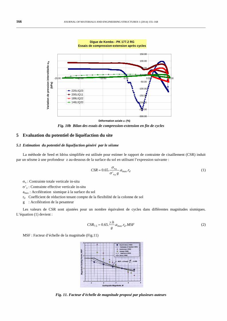
166 JOURNAL OF MATERIALS AND ENGINEERING STRUCTURES 1 (2014) 155–168
Fig. 10b Bilan des essais de compression-extension en fin de cycles
5 Evaluation du potentiel de liquéfaction du site
5.1 Estimation du potentiel de liquéfaction généré par le séisme
La méthode de Seed et Idriss simplifiée est utilisée pour estimer le rapport de contrainte de cisaillement (CSR) induit par un séisme à une profondeur z au-dessous de la surface du sol en utilisant l’expression suivante :
d
ov
ov rag
CSR ..'
.65.0 maxσσ
= (1)
σo : Contrainte totale verticale in-situ σ’o : Contrainte effective verticale in-situ amax : Accélération sismique à la surface du sol rd Coefficient de réduction tenant compte de la flexibilité de la colonne de sol g : Accélération de la pesanteur
Les valeurs de CSR sont ajustées pour un nombre équivalent de cycles dans différentes magnitudes sismiques. L’équation (1) devient :
MSFraghCSR d .....65.0 max5.7
γ= (2)
MSF : Facteur d’échelle de la magnitude (Fig.11)
Fig. 11. Facteur d’échelle de magnitude proposé par plusieurs auteurs
Digue de Kembs - PK 177.2 RGEssais de compression-extension après cycles
-300.00
-250.00
-200.00
-150.00
-100.00
-50.00
0.00
50.00
100.00
150.00
-20.00 -15.00 -10.00 -5.00 0.00 5.00
Déformation axiale ε1 (%)
Varia
tion
de p
ress
ion
inte
rstit
ielle
uB
(kPa
)
220LIQ23200LIQ11189LIQ22146LIQ20
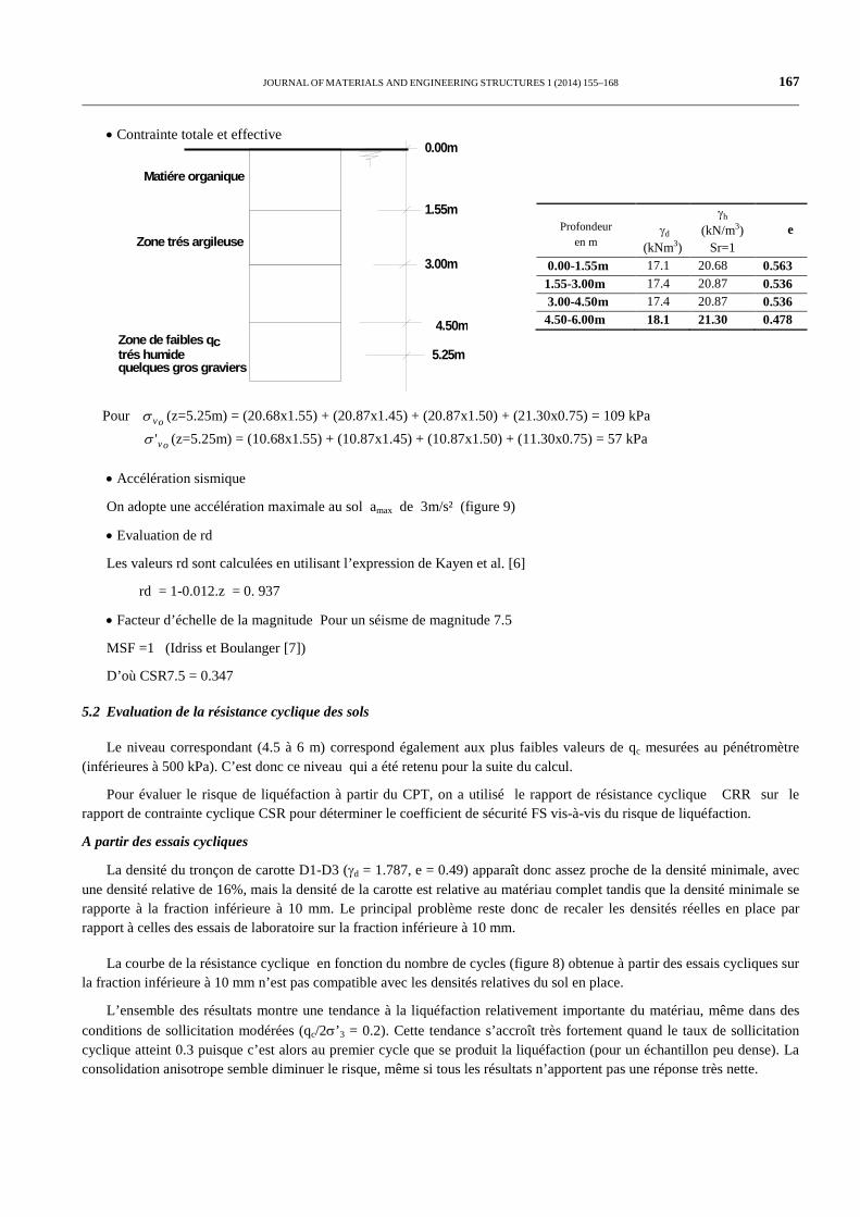
JOURNAL OF MATERIALS AND ENGINEERING STRUCTURES 1 (2014) 155–168 167
• Contrainte totale et effective
Pour ovσ (z=5.25m) = (20.68x1.55) + (20.87x1.45) + (20.87x1.50) + (21.30x0.75) = 109 kPa ov'σ (z=5.25m) = (10.68x1.55) + (10.87x1.45) + (10.87x1.50) + (11.30x0.75) = 57 kPa • Accélération sismique
On adopte une accélération maximale au sol amax de 3m/s² (figure 9)
• Evaluation de rd
Les valeurs rd sont calculées en utilisant l’expression de Kayen et al. [6]
rd = 1-0.012.z = 0. 937
• Facteur d’échelle de la magnitude Pour un séisme de magnitude 7.5
MSF =1 (Idriss et Boulanger [7])
D’où CSR7.5 = 0.347
5.2 Evaluation de la résistance cyclique des sols
Le niveau correspondant (4.5 à 6 m) correspond également aux plus faibles valeurs de qc mesurées au pénétromètre (inférieures à 500 kPa). C’est donc ce niveau qui a été retenu pour la suite du calcul.
Pour évaluer le risque de liquéfaction à partir du CPT, on a utilisé le rapport de résistance cyclique CRR sur le rapport de contrainte cyclique CSR pour déterminer le coefficient de sécurité FS vis-à-vis du risque de liquéfaction.
A partir des essais cycliques
La densité du tronçon de carotte D1-D3 (γd = 1.787, e = 0.49) apparaît donc assez proche de la densité minimale, avec une densité relative de 16%, mais la densité de la carotte est relative au matériau complet tandis que la densité minimale se rapporte à la fraction inférieure à 10 mm. Le principal problème reste donc de recaler les densités réelles en place par rapport à celles des essais de laboratoire sur la fraction inférieure à 10 mm.
La courbe de la résistance cyclique en fonction du nombre de cycles (figure 8) obtenue à partir des essais cycliques sur la fraction inférieure à 10 mm n’est pas compatible avec les densités relatives du sol en place.
L’ensemble des résultats montre une tendance à la liquéfaction relativement importante du matériau, même dans des conditions de sollicitation modérées (qc/2σ’3 = 0.2). Cette tendance s’accroît très fortement quand le taux de sollicitation cyclique atteint 0.3 puisque c’est alors au premier cycle que se produit la liquéfaction (pour un échantillon peu dense). La consolidation anisotrope semble diminuer le risque, même si tous les résultats n’apportent pas une réponse très nette.
Profondeur
en m
γd
(kNm3)
γh
(kN/m3) Sr=1
e
0.00-1.55m 17.1 20.68 0.563 1.55-3.00m 17.4 20.87 0.536 3.00-4.50m 17.4 20.87 0.536 4.50-6.00m 18.1 21.30 0.478
0.00m
1.55m
3.00m
4.50mZone de faibles qctrés humidequelques gros graviers
Matiére organique
Zone trés argileuse
5.25m

168 JOURNAL OF MATERIALS AND ENGINEERING STRUCTURES 1 (2014) 155–168
A partir du CPT (Cone Penetration Test)
Pour le CPT, le rapport de résistance cyclique est donné par Youd et al. [8]. Il s’exprime en fonction de la résistance normalisée qC1N. L’évaluation du potentiel de liquéfaction pour une résistance de 500 kPa au CPT, montre un très grand risque de liquéfaction (Tableau 3). Ce résultat est encore plus vrai pour des valeurs inférieures à cette résistance.
Table 3. Evaluation du facteur de sécurité
[1] [2] [3] [4] [5] [6] [7] [9]
Depth σv rd CSR qC1N CRR σ'v FS
(m) kN/m² kN/m²
5.25 109.6 0,937 0.347 5.6 0,05 560 0.15
6 Conclusion
L’ensemble des essais réalisés sur le matériau de la digue de Kembs apparaissent assez cohérents entre eux, mais pas du tout avec la densité en place déduite des carottes. La densité minimale de 1.91 mesurée par la procédure normalisée sur les échantillons de matériau complet (c’est-à-dire comportant 70% de particules supérieures à 10 mm) n’est pas compatible avec les densités de 1.8 à 1.9 déduites des poids des morceaux de carottes. Le principal problème reste donc de recaler les densités réelles en place par rapport à celles des essais de laboratoire sur la fraction inférieure à 10 mm.
L’ensemble des résultats montre une tendance à la liquéfaction relativement importante du matériau, même dans des conditions de sollicitations modérées (qc/2σ’3 = 0.2). Cette tendance s’accroît très fortement quand le taux de sollicitation cyclique atteint 0.3 puisque c’est alors au premier cycle que se produit la liquéfaction (pour un échantillon peu dense). La consolidation anisotrope semble diminuer le risque, même si tous les résultats n’apportent pas une réponse très nette.
L’essai au CPT montre également une grande tendance à la liquéfaction avec un coefficient de sécurité largement inférieur à 1.
REFERENCES
[1]- G. Bambara, N. Benahmed, P. Mériaux, O. Bellier, Première caractérisation du risque de liquéfaction sous sollicitation sismique d’ouvrages hydraulique en remblai existants ou projetés en basse vallée du Rhône. In : Digues Maritimes et Fluviales de Protection contre les Submersions, 2ème colloque national, Lavoisier, 2013.
[2]- H.B. Seed, I.M. Idriss, Simplified procedure for evaluating soil liquefaction potential. J. Soil Mech. Foundation Div-ASCE, 97(9)(1971) 1249-1273.
[3]- Y.P. Vaid, J.C. Chern, Effects of static shear on resistance to liquefaction. Soils and foundations, 23(1983) 47-60. [4]- H.B. Seed, L.K. Lee, Liquefaction of saturated sands during cyclic load. J. Soil Mech. Foundation Div-ASCE.
92(6)(1966) 105-134. [5]- T.F. Vilela, Mesure des propriétés rhéologiques du sol en régime non permanent ou cyclique. Thèse Docteur
Ingénieur, Ecole Centrale de Paris, 1979. [6]- R.E. Kayen, J.K. Mitchell, A. Lodge, R.B. Seed, S. Nishio, R. Coutinho, Evaluation of SPT, CPT, and shear wave
methods of liquefaction potential assessments using Loma Prieta data. In: Proceedings of the 4th Japan–U.S. Workshop on Earthquake Resistant Design of Lifeline Facilities and Countermeasures for Soil Liquefaction. Technical Report NCEER-92-0019, National Center for Earthquake Engineering Research, Buffalo, N.Y. 177-204, 1992.
[7]- I.M. Idriss, R.W. Boulanger, Semi-empirical Procedures for Evaluating Liquefaction Potential during Earthquakes. Soil Dyn. Earthq. Eng. - 11th International Conference on Soil Dynamics and Earthquake Engineering (ICSDEE): Part II 26(2-4)(2006) 115-130.
[8]- T.L. Youd, I.M. Idriss, R.D. Andrus, I. Arango, G. Castro, J.T. Christian, R. Dobry, W.D.L. Finn, L.F. Harder Jr., M.E. Hynes, K. Ishihara, J.P. Koester, S.S.C. Liao, W.F. Marcuson III, G.R. Martin, J.K. Mitchell, Y. Moriwaki, M.S. Power, P.K. Robertson, R.B. Seed, K.H. Stokoe II. Liquefaction Resistance of soils: Summery report from the 1996 NCEER and 1998 NCEER/NSF workshops on evaluation of liquefaction resistance of soils. J. Geotech. Geoenviron. Eng. 127(10)(2001) 817-833.