Formation of hexagonal pattern of ferrofluid in magnetic field

Yuan Cao, Z.J. Ding n

Hefei National Laboratory for Physical Sciences at Microscale and Department of Physics, University of Science and Technology of China, Hefei, Anhui 230026, China

a r t i c l e i n f o

Article history:Received 4 September 2013Received in revised form14 October 2013Available online 28 November 2013

Keywords:FerrofluidFinite element methodPattern formation

a b s t r a c t

Simulation of hexagonal pattern formation of ferrofluid in magnetic field has been performed using afinite element method. Based on simulation result, a new mechanism involving ‘active rings’ is proposedto explain the generation of new peaks. Hexagonal nature of the pattern is shown to be originated fromthe intersections of these active rings. Evidence of this active ring mechanism is demonstrated andvisualized with patterns grown in strong magnetic field. Calculated single peak profile also agrees wellwith experimental measurements.

& 2013 Elsevier B.V. All rights reserved.

1. Introduction

Ferrofluids are magnetic particles (usually magnetite) sus-pended uniformly in a non-magnetic carrier fluid. If a uniformand vertical magnetic field is applied on a ferrofluid, a pattern ofpeaks would emerge on the surface when the field strength isabove a critical value Bc [1–3]. This phenomenon, namely Rosens-weig or normal field instability, is hysteretic near the transitionpoint. According to Rosensweig's linear stability analysis of mag-netic fluids, the minimum requirement for magnetization strengthMc for the generation of a pattern is predicted to be

M2c ¼

2μ0

1þ 1r0

� � ffiffiffiffiffiffiffiffiffiρgs

p; ð1Þ

r0 ¼ffiffiffiffiffiffiffiffiffiffiμcμt

p=μ0; μc ¼ B=H; μt ¼ ∂B=∂H; ð2Þ

where constants ρ and s denote the density and surface tension offerrofluid, respectively. Here μc and μt are both relative perme-abilities. With a known magnetization relationship of the ferro-fluid, one can compute the critical field Bc as

Bc ¼ μ0½HðMcÞþMc�: ð3Þ

It is necessary to emphasize that the critical value only acts as alower limit for the stable existence of pattern. The actual magneticfield for the onset of the instability might be higher than thecritical value and sensitive to environment such as boundariesdue to hysteresis character of the system. It is also predicted thatthe instability is associated with wave number selection above thecritical field [4]. Only interfacial waves that have a wave numbernear kc ¼

ffiffiffiffiffiffiffiffiffiffiffiρg=s

pcould possibly exist on the surface of a ferrofluid.

This critical wave number equals the capillary wave number of the

fluid. For this reason, the corresponding wavelength λc ¼ 2π=kc isan important length scale for this particular system.

Above a second magnetic field threshold, the ferrofluid systemexhibits a hexagon-square pattern transition [5,6]. Hexagon-squarepattern transition is not unique in the ferrofluid system, but has alsobeen observed in several other systems experimentally, such asRayleigh–Bénard convection [7]. All these transitions and instabilitiescan be analyzed with a generalized Swift–Hohenberg equation [8].However within the regime of linear stability analysis, the amplitudeof the pattern must be small enough compared with the character-istic length scale of the system, λc, in order to utilize perturbationapproximation. Unfortunately the pattern amplitude in ferrofluids isoften in the same order of magnitude with λc in reality. Furthermore,no information about the peak shape or dynamical process of thepeak formation can be obtained with a stability analysis.

Numerical methods have the advantage that any complicatedsystem could be simulated provided with a reasonable model and aset of equations. Several numerical methods for ferrofluid computa-tion have been proposed. One of the most generalized method is thefinite element method which has been employed to solve a largecategory of linear and non-linear partial differential equations. Finiteelement calculation of the ferrofluid system agrees well withexperimental data [9–11]. Some variations of the finite elementmethod are also proposed [12], but the calculations are either coarseor time consuming. In this paper we investigate the pattern forma-tion by finite element computations. As the single peak profile hasalready been studied [9], this work focuses on multi-peak patternformation. The calculated single peak profile is also compared withtheoretical and experimental data.

2. Numerical method

The ferrofluid system follows the Navier–Stokes equationwhich governs the movement of any viscous and compressible

Contents lists available at ScienceDirect

journal homepage: www.elsevier.com/locate/jmmm

Journal of Magnetism and Magnetic Materials

0304-8853/$ - see front matter & 2013 Elsevier B.V. All rights reserved.http://dx.doi.org/10.1016/j.jmmm.2013.11.042

n Corresponding author. Tel.: þ86 86 551 63601857.E-mail address: zjding@ustc.edu.cn (Z.J. Ding).

Journal of Magnetism and Magnetic Materials 355 (2014) 93–99

fluid, while the magnetic force which is determined by thesolution of Maxwell equations in ferrofluids must be included inthe body force term in the Navier–Stokes equation. On the inter-face between the ferrofluid and its surroundings (usually air), theeffect of surface tension has to be taken into consideration as well,which can be described by the Young–Laplace equation. In thisnumerical computation only the equilibrium surface topographyand slow movements are considered, thus the quasi-static approx-imation (u� 0) could be made. Specifically, the incompressibleNavier–Stokes equation with non-zero velocity field u and viscos-ity η can be written as

ρ∂u∂t

¼ �ρðu �∇Þu�∇pþη∇2uþ f b; ð4Þ

∇ � u¼ 0; ð5Þwhere the pressure p¼ phþpm includes contribution from hydro-static pressure ph as well as magnetic pressure pm ¼ μ0

RH0 MðhÞ dh.

Eq. (5) implies the incompressibility of the fluid. f b in Eq. (4)denotes the body force applied to the fluid, which in the case of aferrofluid is

f b ¼ �ρgezþμ0M∇H�μ0∇Z H

0MðhÞ dh

� �: ð6Þ

Limited to quasi-static situation, the Navier–Stokes equation issimplified to

∇p¼ �ρgezþμ0M∇H�μ0∇Z H

0MðhÞ dh

� �: ð7Þ

On the ferrofluid surface, the Young–Laplace equation reads

p�p0 ¼ sK; ð8Þwhere p0 is the atmosphere pressure, s is the surface tension, andK denotes the surface mean curvature. If the fluid surface could berepresented with a single-valued function of horizontal position,that is z¼ zðx; yÞ, K can be written analytically as

K ¼ �∇ � ∇zffiffiffiffiffiffiffiffiffiffiffiffiffiffiffiffiffiffiffi1þð∇zÞ2

q0B@

1CA: ð9Þ

Integration of Eq. (7) and substitution with the Young–Laplaceequation yields [3]

sKþρgzþpr ¼ μ0

Z H

0MðhÞ dhþμ0

2M2

n; ð10Þ

where pr is a reference pressure that can be determined byconservation of fluid volume.

On the other hand, the magnetic field strength and magnetiza-tion in the ferrofluid at any time could be determined by Maxwellequations with an appropriate boundary condition. With magneticpotential φm introduced, the equation above becomes

�∇ � ðμ∇φmÞ ¼ 0; H ¼ �∇φm: ð11ÞSince ferrofluids cannot be treated as linearly magnetized under astrong field, the Langevin equation must be incorporated toaccurately describe the magnetization of ferrofluids. In the formof magnetic permeability μ, the equation reads

μðHÞ ¼ 1þMs

H1

tanhðγHÞ �1γH

� �ferrofluid

1 air:

8<: ð12Þ

Here γ ¼ 3χ0=Ms, initial susceptibility χ0 and magnetization para-meter Ms are all constants at a certain temperature.

The simulation of the static surface topography of a ferrofluidis performed in two-stage cycles. The initial surface of each cycleis given by the result of the last cycle. Three-dimensional meshesare generated in the two domains (air and ferrofluid) defined by

this flexible surface and the fixed boundaries. In the first stage, themagnetic potential and the magnetic field strength in Eq. (11) aresolved with a 3-D finite elements solver. Since the system can onlybe provided with an all-Neumann boundary condition, an addi-tional Lagrange multiplier have to be integrated into the resultingstiffness matrix as an independent variable, in order to avoidundesirable outcome resulting from the impossibility to determinean absolute magnetic potential [13]. In the second stage, zðx; yÞ inEq. (10) is solved using a 2-D finite elements solver. In this stage allright-hand terms in Eq. (10) are regarded as constants, that are theresults of the first stage. It should be noticed that both stagesinvolve non-linearity, the first stage from the non-linearity of themagnetization equation, Eq. (12) and the second stage from theexpression of the mean curvature, Eq. (9). These non-linearitiescan be resolved by fixed-point iterations independently in bothstages. The spatial domain considered here is either a hexagonal ora square prism. In both stages, periodic boundary condition is seton all side faces of the prism, while the magnetic field is imposedon the system by setting a non-zero Neumann condition on thetop and bottom faces of the prism.

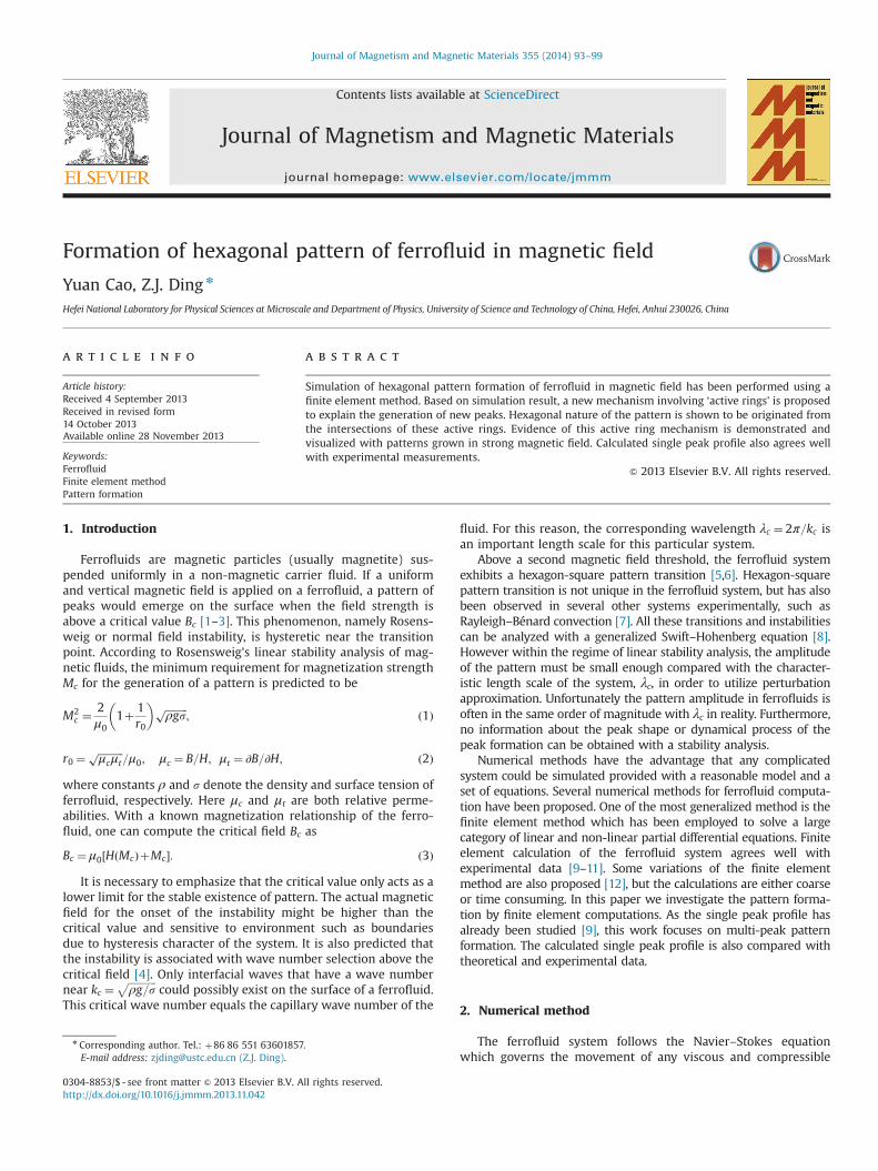
All of the algorithm described above are implemented in asingle program of FreeFemþþ finite element programminglanguage [14]. The material parameters of the ferrofluid areset to the same as in Ref. [9], for comparison with an experimentalresult. These parameters are listed in Table 1. An example ofthe simulated single peak surface and multi-peak pattern is shownin Fig. 1.

3. Results and discussion

3.1. Single peak

The single peak simulation is carried out in a hexagonaldomain. We considered a periodic boundary condition on the sidefaces of the prism instead of the Neumann condition used in Ref.[9], for consistency with the multi-peak simulation that will bediscussed later, where only periodic boundaries can be used. Forthe single peak simulation, the outcomes of these two kinds ofboundary conditions are basically identical. The domain size isset such that its periodic extension would have a wave numberexactly equal to kc ¼ ðρg=sÞ1=2 ¼ 0:629 mm�1, the maximum pos-sible wave number for any stable ferrofluid system. The side lengthof such hexagonal domain is therefore 2π=

ffiffiffi3

pkc ¼ 5:77 mm. For

comparison with different systems, a bifurcation parameter ɛ isusually introduced to describe the relative strength of the externalmagnetic induction, which is defined as

ɛ¼ B2�B2c

B2c

: ð13Þ

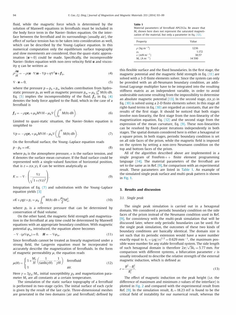
The effect of magnetic induction on the peak height (i.e. thedifference of maximum and minimum z-values of the interface) isplotted in Fig. 2 and compared with the experimental result fromRef. [9]. In the simulation result, Bc¼18.23 mT is found to be thecritical field of instability for our numerical result, whereas the

Table 1Material parameters of ferrofluid APG512a. Be aware thatMs shown here does not represent the saturated magneti-zation of the material, but only a parameter in Eq. (12).

Property Value

ρ (kg m�3) 1236χ0 1.172s (mN m�1) 30.57Ms (A m�1) 14 590

Y. Cao, Z.J. Ding / Journal of Magnetism and Magnetic Materials 355 (2014) 93–9994

critical value in experiment is 16.747 mT, slightly lower than bothour value and the theoretical prediction at 17.22 mT given by Eq.(1) using the parameters in Table 1. In Fig. 2, we have used18.23 mT and 16.747 mT as critical field Bc to calculate thebifurcation parameters for the numerical and experimental datarespectively. The calculated critical value is noticeably deviatedfrom the theoretical value, which is because we set the boundarycondition on top and bottom faces differently from that in linearstability analysis. Both the linear stability analysis of Rosensweigand the simulation in [9] set a Dirichlet condition of φm ¼ 7zHe

on the top and bottom faces of the domain respectively, where He

is the external magnetic field. However this is not valid in ourmulti-peak simulation because of its large peak amplitude. There-fore we use the Neumann condition that was described in Section2 on the top and bottom faces, which gives limitations only on thenormal derivative ∂φm=∂n but not φm itself. For consistency, thisboundary condition is also used for the single peak simulation, andthe cost of doing this is a deviation from the result of linearstability analysis.

Another theoretical stability analysis [4] gives a formula for thepeak height versus ɛ in a hexagonal pattern,

h¼ Abð1þɛÞþ

ffiffiffiffiffiffiffiffiffiffiffiffiffiffiffiffiffiffiffiffiffiffiffiffiffiffiffiffiffiffiffiffiffib2ð1þɛÞ2þ4aɛ

q2a

ð14Þ

where a, A and b are parameters to fit the data from either thenumerical or the experimental result. The fitting curve for ournumerical data is plotted as a blue line in Fig. 2, with theparameters a¼0.002 65, b¼0.002 93 and A¼ 3:15� 10�4.

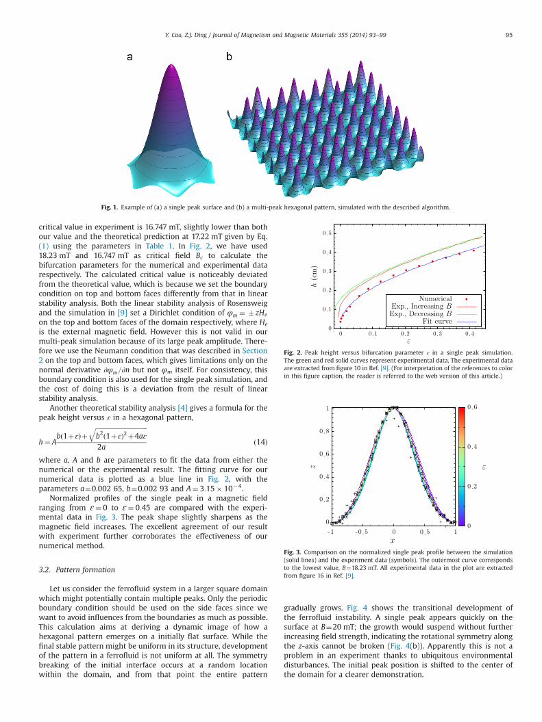
Normalized profiles of the single peak in a magnetic fieldranging from ɛ ¼ 0 to ɛ ¼ 0:45 are compared with the experi-mental data in Fig. 3. The peak shape slightly sharpens as themagnetic field increases. The excellent agreement of our resultwith experiment further corroborates the effectiveness of ournumerical method.

3.2. Pattern formation

Let us consider the ferrofluid system in a larger square domainwhich might potentially contain multiple peaks. Only the periodicboundary condition should be used on the side faces since wewant to avoid influences from the boundaries as much as possible.This calculation aims at deriving a dynamic image of how ahexagonal pattern emerges on a initially flat surface. While thefinal stable pattern might be uniform in its structure, developmentof the pattern in a ferrofluid is not uniform at all. The symmetrybreaking of the initial interface occurs at a random locationwithin the domain, and from that point the entire pattern

gradually grows. Fig. 4 shows the transitional development ofthe ferrofluid instability. A single peak appears quickly on thesurface at B¼20 mT; the growth would suspend without furtherincreasing field strength, indicating the rotational symmetry alongthe z-axis cannot be broken (Fig. 4(b)). Apparently this is not aproblem in an experiment thanks to ubiquitous environmentaldisturbances. The initial peak position is shifted to the center ofthe domain for a clearer demonstration.

Fig. 1. Example of (a) a single peak surface and (b) a multi-peak hexagonal pattern, simulated with the described algorithm.

Fig. 2. Peak height versus bifurcation parameter ɛ in a single peak simulation.The green and red solid curves represent experimental data. The experimental dataare extracted from figure 10 in Ref. [9]. (For interpretation of the references to colorin this figure caption, the reader is referred to the web version of this article.)

Fig. 3. Comparison on the normalized single peak profile between the simulation(solid lines) and the experiment data (symbols). The outermost curve correspondsto the lowest value, B¼18.23 mT. All experimental data in the plot are extractedfrom figure 16 in Ref. [9].

Y. Cao, Z.J. Ding / Journal of Magnetism and Magnetic Materials 355 (2014) 93–99 95

Only after a process of ‘magnetic annealing’, i.e. firstly increasingthe field to B¼24 mT and iterate until further instability emerges(Fig. 4(c)), and then cooling the system down to B¼20 mT, an initialpattern forms around the first peak (Fig. 4(d)). Note that this initialpattern is not hexagonal, but rather heptagonal or even octagonal insome cases. A possible explanation is that the symmetry-breakingby the annealing process leads to a metastable state at a localenergy minimum. Therefore, seven peaks can coexist in a ringaround the initial single peak.

Subsequent popping out of new peaks around the initialpattern at B¼23 mT (Fig. 4(e–h)) generates a quasi-hexagonalpattern of the system, with the initial peak being an heptagonalimperfection in the pattern. New peaks tend to form at thepositions that allow as many equilateral triangles with other peaksas possible. As a consequence, pattern formed in this way tends tobe a hexagonal lattice. The initial heptagonal pattern is anexception because it is not generated by an existing pattern butonly a single peak.

Fourier filtering of the data in Fig. 4(h) is performed anddisplayed in Fig. 5. Along different directions, the filtered imagesclearly show a quasi-periodic structure, with partial distortionsgenerated by the heptagonal imperfection at the domain center.Apart from the central area, the pattern is locally hexagonal at allpositions in the domain. Analysis of the filtered images gives awave number of the pattern at 0.482 mm�1, which is 23% smallerthan the capillary wave number kc ¼ ðρg=sÞ1=2 ¼ 0:629 mm�1. Thisdifference is primarily a result of the lack of solid non-periodicboundaries that could induce lateral pressure on the peaks andthus forming a denser pattern. The disorder and defects alsocontribute to the wave number difference. A cross-section of thepeaks in the stable pattern is plotted in Fig. 6.

The area of peaks is noticeably smaller than that of valleys. Inboth theories [4,16] and experiments [9,15], however, the patterncan be presumably described by the sum of three sinusoidalfunctions defined by three wave vectors that have angles of 1201with each other, i.e.

zðrÞ ¼ Að sin ðk1 � rÞþ sin ðk2 � rÞþ sin ðk3 � rÞÞ: ð15ÞPatterns determined by this formula have uniform peak and

valley sizes. The deviation of our numerical result from thisformula implies the possibility of the pattern realigning itself tobe more compact. In the present work we only show the way howthe pattern forms on a ferrofluid in a domain free of interferences

Fig. 4. Snapshots of evolution of pattern in a domain with square boundary. Magnetic field and iteration cycle number t for each snapshot is labeled in each graph.Bar in (a) equals 2 cm.

Fig. 5. Fourier filtered image of Fig. 4(h) along different directions.

Fig. 6. Cross-section of the peak profile in the pattern along the red line in theinset. (For interpretation of the references to color in this figure caption, the readeris referred to the web version of this article.)

Y. Cao, Z.J. Ding / Journal of Magnetism and Magnetic Materials 355 (2014) 93–9996

from the container sides, when it is exposed to a uniform magneticfield.

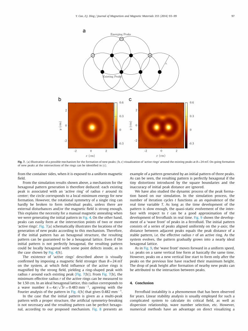
From the simulation results shown above, a mechanism for thehexagonal pattern generation is therefore deduced: each existingpeak is associated with an ‘active ring’ of radius r around itscenter; the circle corresponds to a local minimum energy for newformation. However, the rotational symmetry of a single ring canhardly be broken to form individual peaks, unless there areexternal disturbances and/or the magnetic field is strong enough.This explains the necessity for a manual magnetic annealing whenwe were generating the initial pattern in Fig. 4. On the other hand,peaks can easily form at the intersection points of two or more‘active rings’. Fig. 7(a) schematically illustrates the locations of thegeneration of new peaks according to this mechanism. Therefore,if the initial pattern has an hexagonal structure, the resultingpattern can be guaranteed to be a hexagonal lattice. Even if theinitial pattern is not perfectly hexagonal, the resulting patterncould be locally hexagonal with some point defects inside, as inthe case shown by Fig. 4(h).

The existence of ‘active rings’ described above is visuallyconfirmed by imposing a magnetic field stronger than B¼24 mTon the system, at which field influence of the active rings ismagnified by the strong field, yielding a ring-shaped peak withradius r around each existing peak (Fig. 7(b)). From Fig. 7(b), theminimum effective radius r of the active rings can be measured tobe 1.50 cm. In an ideal hexagonal lattice, this radius corresponds toa wave number k¼ 4π=

ffiffiffi3

pr¼ 0:483 mm�1, agreeing with the

Fourier analysis of the pattern in Fig. 4(h) that gives 0.482 mm�1.In the case that the initial pattern is given as a multi-peak

pattern with a proper structure, the artificial symmetry-breakingis not necessary and the resulting pattern can be perfect hexago-nal, according to our proposed mechanism. Fig. 8 presents an

example of a pattern generated by an initial pattern of three peaks.As can be seen, the resulting pattern is perfectly hexagonal if thetiny distortions introduced by the square boundaries and theinaccuracy of initial peak distance are ignored.

We have also studied the dynamic process of the peak forma-tion based on our simulation. In the simulation process, thenumber of iteration cycles t functions as an equivalence of thereal time variable T. As long as the time development of thepattern is slow enough, the quasi-static evolvement of the inter-face with respect to t can be a good approximation of thedevelopment of ferrofluids in real time. Fig. 9 shows the develop-ment of a ‘wave front’ of peaks in a ferrofluid. The initial patternconsists of a series of peaks aligned uniformly on the y-axis; thedistance between adjacent peaks equals the peak distance of astable pattern, i.e. the effective radius r of an active ring. As thesystem evolves, the pattern gradually grows into a nearly idealhexagonal lattice.

As in Fig. 9, the ‘wave front’ moves forward in a uniform speed,i.e. peaks on a same vertical line form at basically the same time.However, peaks on a new vertical line start to form only after thepeaks on the previous line have reached their maximum height.The drop of peak height after formation of nearby new peaks canbe attributed to the interaction between peaks.

4. Conclusion

Ferrofluid instability is a phenomenon that has been observedfor years. Linear stability analysis is usually employed for such acomplicated system to calculate its critical field, as well asdispersion relationship, wave number selection, etc. However,numerical methods have an advantage on direct visualizing a

Fig. 7. (a) Illustration of a possible mechanism for the formation of new peaks; (b, c) visualization of ‘active rings’ around the existing peaks at B¼24 mT. On-going formationof new peaks at the intersections of the rings can be identified in (c).

Y. Cao, Z.J. Ding / Journal of Magnetism and Magnetic Materials 355 (2014) 93–99 97

physical phenomenon. We demonstrate here how a hexagonalpattern on ferrofluid is generated in real world, by a way of directcomputation with the finite element method. A new mechanismfor the formation of hexagonal patterns in ferrofluids is proposedbased on the numerical results.

The hexagonal pattern is not an effect of the boundaries as asquare domain can generate a hexagonal as well. It is an equili-brium state of a ferrofluid system at which state an energyminimum is maintained under applied magnetic field. In a certainmagnetic field, peaks tend to form at the intersections of the activerings around the existing peaks, and a pattern grew in this waynaturally exhibits a hexagonal structure.

In our numerical result we have also found the stable patternfrom simulation is not the most compact form for the peaks inreality, with its primary wave number noticeably lower than the

experimental results and theoretical predictions. This phenomenoninvolves horizontal movement and rearrangement of the peaks, thusrequiring much more iteration cycles and computation.

Acknowledgments

This work was supported by the National Natural Science Founda-tion of China (Grant nos. 11074232 and 11274288), the National BasicResearch Program of China (nos. J1103207, 11074232 and 11274288),Ministry of Education of China (no. 20123402110034), ChineseAcademy of Sciences (no. XXH12503-02-02-07) and ‘111’ project(no. B07033). We thank the Supercomputing Center of USTC for thesupport in performing parallel computations.

Fig. 8. A perfect pattern generated by three peaks. (a) Initial pattern; (b) final pattern.

Fig. 9. Development of ferrofluid peak ‘wave front’. (a) The initial pattern; (b) the pattern after t¼192 iteration cycles; (c) the evolvement of peak heights of six peaks labeledin (b), with respect to t. Each iteration cycle is the two-stage process as described in Section 2.

Y. Cao, Z.J. Ding / Journal of Magnetism and Magnetic Materials 355 (2014) 93–9998

Appendix A. Supplementary material

Supplementary data associated with this article can be found inthe online version of http://dx.doi.org/10.1016/j.jmmm.2013.11.042.

References

[1] M.D. Cowley, R.E. Rosensweig, The interfacial stability of a ferromagnetic fluid,J. Fluid Mech. 30 (1967) 671–688.

[2] A. Gailitis, Formation of the hexagonal pattern on the surface of a ferromag-netic fluid in an applied magnetic field, J. Fluid Mech. 82 (1977) 401–413.

[3] R.E. Rosensweig, Ferrohydrodynamics, Courier Dover Pub., 1997.[4] R. Friedrichs, A. Engel, Pattern and wave number selection in magnetic fluids,

Phys. Rev. E 64 (2001) 021406.[5] C. Gollwitzer, R. Rehberg, R. Richter, Via hexagons to squares in ferrofluids:

experiments on hysteretic surface transformations under variation of thenormal magnetic field, J. Phys. Condens. Matter 18 (2006) S2643.

[6] B. Abou, J.E. Wesfreid, S. Roux, The normal field instability in ferrofluids:hexagon–square transition mechanism and wavenumber selection, J. FluidMech. 416 (2000) 217–237.

[7] K. Nitschke, A. Thess, Secondary instability in surface-tension-driven Bénardconvection, Phys. Rev. E 52 (1995) R5772–R5775.

[8] C. Kubstrup, H. Herrero, C. Perez-Garcia, Fronts between hexagons and squaresin a generalized Swift–Hohenberg equation, Phys. Rev. E 54 (1996) 1560–1569.

[9] C. Gollwitzer, G. Matthies, R. Richter, I. Rehberg, L. Tobiska, The surfacetopography of a magnetic fluid: a quantitative comparison between experi-ment and numerical simulation, J. Fluid Mech. 571 (2007) 455–474.

[10] G. Matthies, L. Tobiska, Numerical simulation of normal-field instability in thestatic and dynamic case, J. Mag. Mag. Mater. 289 (2005) 346–349.

[11] C. Gollwitzer, A.N. Spyropoulos, A.G. Papathanasiou, A.G. Boudouvis, R. Richter,The normal field instability under side-wall effects: comparison of experi-ments and computations, New J. Phys. 11 (2009) 053016.

[12] G. Yoshikawa, K. Hirata, F. Miyasaka, Y. Okaue, Numerical analysis of transi-tional behavior of ferrofluid employing MPS method and FEM, Mag. IEEETrans. 47 (2011) 1370–1373.

[13] P. Bochev, R.B. Lehoucq, On finite element discretizations of the pureNeumann problem, SIAM Rev. 47 (2005) 50–66.

[14] F. Hecht, O. Pironneau, A. Le Hyaric, K. Ohtsuka, FreeFemþþ , Laboratoire JLLions, University of Paris VI, 1998.

[15] A.G. Boudouvis, J.L. Puchalla, L.E. Scriven, R.E. Rosensweig, Normal fieldinstability and patterns in pools of ferrofluid, J. Mag. Mag. Mater. 65 (1987)307–310.

[16] A. Lange, B. Reimann, R. Richter, Wave number of maximal growth in viscousmagnetic fluids of arbitrary depth, Phys. Rev. E 61 (2000) 5528–5539.

Y. Cao, Z.J. Ding / Journal of Magnetism and Magnetic Materials 355 (2014) 93–99 99