Journal of International Economics 124 (2020) 103300

Contents lists available at ScienceDirect

Journal of International Economics

j ourna l homepage: www.e lsev ie r .com/ locate / j i e

Written for the NBER International Seminar on Macroeconomics

Price discrimination within and across EMU markets: Evidence fromFrench exporters☆

François Fontaine a, Julien Martin b, Isabelle Mejean c,⁎a Paris School of Economics, Université Paris Panthéon Sorbonne, Franceb Université du Québec à Montréal, CEPR, Canadac CREST-Ecole Polytechnique, CEPR, France

☆ Weare grateful to Brent Neiman, Ida Hjortsoe, CharlesJordi Gali, and participants at theNBER-ISOM conference foThibault Cezanne for excellent research assistance. Fonfinancial support from the Institut Universitaire de France.support from apublic grant overseen by the FrenchNationaof the “Investissements d'Avenir” program (Idex Grant Agre02, Labex ECODECGrant Agreement No. ANR-11-LABEX-0010-EQPX-17 âĂŞ Centre d'accès sécurisé aux données âĂŞResearch Council (ERC) under the European Union's Horizoprogramme (grant agreement No. 714597).⁎ Corresponding author.

E-mail address: isabelle.mejean@polytechnique.edu (I

https://doi.org/10.1016/j.jinteco.2020.1033000022-1996/© 2020 The Authors. Published by Elsevier B.V

a b s t r a c t

a r t i c l e i n f o

Article history:Received 26 August 2019Received in revised form 13 December 2019Accepted 17 January 2020Available online 23 January 2020

Mendeley Data https://data.mendeley.com/datasets/k8c3wmdj8z/draft?a=c32c2dae-08b8-4f66-b3a5-a6634401cc3c

We study the cross-sectional dispersion of prices paid by EMU importers for French products. We document asignificant level of dispersion in unit values both within product categories across exporters, and within ex-porters across buyers. This latter source of price discrepancies, which we call price discrimination, reflects theability of exporters to sell similar or differentiated varieties of a given product at different prices to differentbuyers. Price discrimination (i) is substantial within the EU, within the euro area, and within EMU countries;(ii) has not decreased over the last two decades; (iii) ismore prevalent among the largest firms and formore dif-ferentiated products; (iv) is lower among retailers and wholesalers; (v) is also observed within almost perfectlyhomogenous product categories, which suggests that a non-negligible share of price discrimination is partly trig-gered by heterogeneous markups rather than quality or composition effects. We then estimate a rich statisticaldecomposition of the variance of prices to shed light on exporters' pricing strategies.© 2020 The Authors. Published by Elsevier B.V. This is an open access article under the CC BY-NC-ND license (http://

creativecommons.org/licenses/by-nc-nd/4.0/).

Keywords:Price discriminationFirm-to-firm trade

1. Introduction

The pricing strategy of exporters is a central element of internationalmacroeconomics. Whether exporters sell differentiated or homogenousproducts and charge the same or different prices across partners locatedin various destinations is key to understand deviations from the law ofone price and to anticipate exporters' reaction to domestic and foreignshocks. In this paper we exploit firm-to-firm data to shed light on thepricing strategies of French exporters. The data cover both final and inter-mediate products sold to different buyers within and across EMU coun-tries. These data enable us to quantify the extent of price discrimination,to analyze the heterogeneity in the pricing behavior across producersand sectors, and to discuss the mechanisms behind price discrimination.

We document a significant level of dispersion in the unit valuescharged by producers across their buyers within the EuropeanMonetary

Engel, Pierre-Olivier Gourinchas,r insightful comments, aswell astaine gratefully acknowledgesMejean gratefully acknowledgesl Research Agency (ANR) as partement No. ANR-11-IDEX-0003-47 andEquipex reference: ANR-CASD) as well as the Europeann 2020 research and innovation

. Mejean).

. This is an open access article under

Union. Price discrimination is prevalent across buyers located in differentcountries, but also across buyers within a country. The data show a largeheterogeneity across French exporters in their propensity to price dis-criminate. Large multiproduct exporters tend to adopt more discrimina-tory pricing strategies. Retailers and small exporters instead charge lessdispersed and sometimes nearly uniform prices. Finally, price dispersionis stronger for more differentiated and more durable products.

These evidence rely on data on the unit prices charged by French ex-porters to their European buyers over 2002–2016 for each of the 9000different product categories of the CN8 trade nomenclature. At thislevel of aggregation, the uncovered price dispersion can be driven byi) exporters charging different unit prices for differentiated varieties ofthe same product, or ii) exporters setting different markups acrosstheir customers of a given variety.1 Whereas, we cannot distinguish be-tween these two forms of discrimination, we show that price discrimi-nation remains substantial for a subset of product categories that offerlittle ground for product differentiation. Focusing on the price per kilo-gram of 200 raw molecular substances, we indeed find a level of pricediscrimination in this subsample that is two third of the price discrimi-nation measured in the whole dataset.

We conclude the paper with an examination of the extent to whichexporters' ability to set high prices on their European partners, together

1 Regarding driver i), differences in variety across buyersmight reflect differences in theattributes of the products (eg. its quality), packaging differences, or differences in themixof varieties purchased by the importer.

the CC BY-NC-ND license (http://creativecommons.org/licenses/by-nc-nd/4.0/).

3 This finding confirms the singular role played by durable goods in open-macroeconomics (see Engel and Wang, 2011; Levchenko et al., 2010).

4 Such extrapolation is arguably heroic because the average difference in the dispersionof prices between homogenous and heterogeneous products is estimated for firms in thechemical industry, which may not be representative of the average firm in the data.

2 F. Fontaine et al. / Journal of International Economics 124 (2020) 103300

with importers' tendency to renegotiate prices on thematch participateto the dispersion of prices within a firm. Estimates recovered from ahigh-dimensional fixed effect model show that prices tend to decreaseover time, within a firm-to-firm relationship, while exporters set highprices on newly met partners. These behaviors suggest that some formof price bargaining occurs between the exporter and her foreignpartner.

These new facts build on a unique dataset on firm-to-firm trade inthe EU. For each of the 9000 products that the data cover, we observea set of export transactions taking place in a given quarter between aparticular French firm and one of its partners in the EU. The data enableus to compare the price strategy of two French exporters selling a sim-ilar product to a given EU destination as well as prices set by the samefirm over different partners. At firm-level, any dispersion in the FOBunit values means exporters set different markups and/or supply differ-entiated varieties of the same product to buyers in their portfolio. Thislevel of dispersion constitutes our measure of price discrimination.2

We start our analysis by quantifying how this source of price dis-crepancies influences the overall variance of prices observed in thedata. To this aim,we construct ameasure of price dispersion at theprod-uct level for each quarter and calculate the extent to which these pricediscrepancies come from different exporters serving European marketsat different mean prices, a “between” component, versus individual ex-porters price discriminating between partners in their portfolio, a“within” component. The level of price dispersion recovered fromthese data is substantial. The mean coefficient of variation of prices inthe EU is as high as 1.3. Two thirds of this dispersion is due to the be-tween component, that is, exporters setting heterogeneous averageprices to serve the same or different partners with potentially differen-tiated products. Still, a third of the cross-sectional variance in prices isattributable to the within-seller dimension, that is, exporters chargingheterogeneous prices across their different clients. The rest of the anal-ysis is dedicated to this specific source of price discrepancies, which werefer to as price discrimination.

Price discrimination is a common practice among French exporters.The median coefficient of variation of prices across buyers purchasingthe same product from a given exporting firm in a specific quarter isas high as 30.5%. This average, however, hides a substantial amount ofheterogeneity. In the limit, 14% of exporters have uniform pricing strat-egies in the EMU, yet thesefirms are relatively small and thus contributelittle to aggregate exports.

Although thewithin-firm price dispersion implies systematic devia-tions from the LOP within the euro area, we also document that pricedispersion at the firm-level is less severe within the EMU than in theoverall EU. Mean differences across country samples within a firm arequantitatively important. Priceswithin the extended EU are, on average,10%more dispersed thanwithin the EU restricted to its 15 oldmembers,whereas they are 14% less dispersed in the EMU than in the EU15. Thesedifferences are in part due to composition effects, within a firm, but weshow the difference is still significant when we use firm-level random-ization to compare prices within and outside of the EMU. This findingconfirms that sharing a common currency causes greater market inte-gration. The level of price dispersion has, however, increased overtime, especially for relatively small firms. The coefficient of variationof prices recovered within a firm was 25% higher in the 2010s than inthe 2000s, a result that is robust to composition effects. This resultgoes against the view that both the increasing integration of Europeanmarkets and new communication technologies should enable con-sumers to arbitrage across goods, which is expected to force the

2 Onemay argue that LOP should be considered at the level of consumer prices, thus in-cluding transportation costs. If arbitrage is strong enough, exporters may be forced to ab-sorb trade costs, which would transmit into heterogeneous fob prices but homogenous cifprices. Consistent with existing evidence based on firm-to-destination export data(e.g., see Manova and Zhang, 2012; Martin, 2012, for Chinese and French data), ourfirm-to-firm fob prices are increasing in distance. This finding suggests that, if anything,the corresponding cif prices should be more dispersed than the fob prices we study.

convergence of prices. Instead, the increasing dispersion of prices ob-served within an exporter over time suggests small exporters in oursamplemanage tomaintain high price discrepancies, potentially thanksto product differentiation.

In a second step, we study how firm and product heterogeneity is re-lated to the degree of price discrimination. Among the characteristicsthat might explain why firms are unequally prone to price discriminat-ing, we find a significant effect of the firm's size and profits. Large multi-product exporters and firms with a greater profitability within theirsector of activity are found to price discriminatemore intensively.Withina firm, the propensity to price discriminate isweaker over the firm's coreproduct. Finally, we find evidence of heterogeneity in price discrepanciesacross sectors. Retailers and wholesalers charge less dispersed pricesthanmanufacturingfirms supplying the same type of products. Price dis-persion is stronger for differentiated products, especially durable ones.3

Along the value chain, price discrimination is more stringent for moredownstreamproducts. This heterogeneitymay explain by systematic dif-ferences in consumers' ability to arbitrage induced by product differenti-ation or the structure of competition in various markets.

The dispersion of prices within a firm is consistent with two poten-tially complementary mechanisms. First, exporters may price discrimi-nate across their partners through product differentiation, forexample, by customizing their product to their customers' needs. Sucha strategy should be especially relevant for differentiated goods, thusthe higher mean dispersion of prices observed for these products. Sec-ond, exporters may sell the same product variety to various buyers atdifferentiated prices, thus adjusting their markup to their buyers' valu-ation for the good. Although the data do not allow us to quantify the rel-ative contribution of both factors to the observed dispersion of prices,we conclude the analysis with two exercises that are meant to digdeeper into the underlying mechanisms of price discrimination. In thefirst exercise, we focus on a sub-sample of roughly 200 chemical prod-ucts that we argue offer very little ground for product differentiation,because they correspond to raw molecular substances. By comparingthe level of price dispersion in this sample and in the rest of the dataset,we can provide some indicative elements regarding the role of productdifferentiation as a source of price discrepancies. In the sample of ho-mogenous products, the mean coefficient of variation is about 10 per-centage points lower than in the control group. The difference issignificant, including when identified within firms selling both homog-enous and differentiated chemical products, controlling for unobservedheterogeneity across firms. Extrapolating these results beyond thechemical industry suggests that about a quarter of the observed pricedispersion is due to product differentiation within a firm.4

The second exercise digs deeper into the pricing strategies of Frenchexporters, using a rich linear model to analyze the determinants of ex-port price levels. Using insights from the labor literature (Abowd et al.,1999),we estimate a price equationwith two-sided unobserved hetero-geneity (seller and buyer) that allows us to characterize the dynamics offirm-to-firm prices, conditional on sellers' and buyers' unobserved het-erogeneity. Results show that firm-to-firm prices tend to decrease withthe age of the buyer-seller relationship, which is consistent with buyersrenegotiating and increasing their share of the transaction's surplus asthey increase their outside options.5 Despite downward price

5 Studying the dynamics of prices within a firm-to-firm relationship is insightful as it al-lows us to dampen composition effects that may drive price dispersion between but alsowithin an exporter. Still, unit values recovered from individual transactionsmay suffer frommeasurement bias since buyersmay adjust the composition of thebundle purchased from aseller over time. The systematic (downward) pattern observed in the corresponding seriesof firm-to-firm unit values suggests that i) either this composition effects evolve over timein thedirection offirms purchasingmore andmore of the lowprice varieties or ii) prices arerenegotiated downward on the match which is our preferred interpretation.

7 Our results are not directly comparable with Cavallo et al. (2014) though, who use ac-tual price data collected from four giant retailers. Their data do not suffer from the mea-surement bias inherent to using FOB unit values, which does drive a significant share ofthe dispersion we observe. Moreover, they solely cover final consumption goods whileour data are recovered frombusiness-to-business relationships, and include products usedfor intermediate consumption purposes. Such relationships display a lot more stickiness,as shown by the fact we observe repeated transactions involving the same partners overtime. These long-term relationships give rise to bargaining, as suggested by our empiricalevidence. Bargaining is itself a source of price discrepancies, in the cross-section.

8 Our paper differ along three dimensions from this paper. First, we work with unit

3F. Fontaine et al. / Journal of International Economics 124 (2020) 103300

renegotiations, the mean price set by French exporters increases overtime. The reason is that more experienced exporters manage to expandtheir portfolio of buyers and charge their new consumers relatively highprices. Interestingly, firms at the top of the distribution of sales in theirsector are especially good at charging new consumers high prices whilesuffering from relatively less pronounced downward price renegotia-tion. We thus offer some insights on the way superstar firms exerttheir market power.

Our data enables us to observe unit values set by seller across differ-ent buyers. As such, our work contributes to the literature on firm-to-firm trade, and to the literature on the pricing strategy of exporters.The literature on firm-to-firm trade has not explored the price dimen-sion yet, and most of the literature on the pricing strategy of exportersuses unit values without the buyer dimension. The main limitation ofour data is that differences in unit values are subject to composition ef-fects, and thus reflect both differences in prices and, possibly, in the(mix of) varieties sold to different buyers..6 Formost product categories,the price dispersionwe document comes both frommarkup differencesand variety differences. Nevertheless, the high level of dispersion wedocument implies that a model where sellers sell the same variety andcharge the samemarkup to all their buyerswould not fit the data.More-over, we also find a high level of dispersion in a sample of chemicalswhere composition biases are likely to be limited, suggesting thatmarkup differences are probably pervasive overall.

Literature review. In addition to the works cited above, this paperpertains to different strands of the literature. Deviations from the LOPare often associated with market segmentation and border effects.Engel and John (1996) document systematic deviations from the LOPusing disaggregated consumer price indices across Canadian and US cit-ies. Using similar data across European cities, the authors do not find ev-idence of price convergence after the introduction of the euro (Engeland Rogers, 2004). Within the car industry, Goldberg and Verboven(2005) find a strong positive impact of the European integration onprice convergence, and aweaker impact on the level of price dispersion.We focus here on the absolute version of the LOP. As in Engel and John(1996), we exploit the granularity of the data in the spatial dimension tocompare the level of price discrepancieswithin the euro area andwithincountries of the euro area.

Part of the literature relates deviations from the LOP at the consumerlevel to the extent of local distribution costs (Crucini et al., 2005; Cruciniand Shintani, 2008). According to Gopinath et al. (2011), these distribu-tion costs are not the main source of price discrepancies, which are in-stead high upstream in the value chain, at the wholesale level. Ouranalysis confirms their result by documenting the large degree ofprice discrepancies at the producer level. The evidence documented inGopinath et al. (2011) further suggests that the price differences wedocument are likely to translate into price discrepancies at the con-sumer price level.

Because our data cover both manufacturing firms and wholesalersand retailers, for a wide range of different products, we can also com-pare the propensity to price discriminate at different points of thevalue chain. Although price discrepancies are large on average in all sec-tors, we do find some evidence of the propensity to price discriminatebeing smaller in the retail sector, within a product. The lower level ofprice discrimination by retailers is consistent with results in Cavalloet al. (2014) on the LOP within the EMU. The paper documents the im-portance of uniform pricing across euro countries for products sold on-line by four large retailers. To our knowledge, this paper is the first to

6 Examples of top product categories in French exports are: Aeroplanes and otherpowered aircraft of anunladenweightN 15.000 kg (excl. helicopters and dirigibles),Motorcars and othermotor vehicles principally designed for the transport of persons (other thanthose of heading No 8702), incl. Stationwagons and racing cars, with spark-ignition inter-nal combustion reciprocating piston engine, of a cylinder capacity N1.500 cm3 but ≤ 3.000cm3, new (excl. 8703.10–10 and 8703.23.11), Motor spirit, with a lead content ≤ 0,013 g/l,with an research octane number “RON” of b95, or Champagne of actual alcoholic strengthof ≥ 8,5% vol.

document uniform pricing across different countries. Although wefind retailers (and non-durable goods) have a lower price dispersionin our data, the prevalence of uniformpricing is not striking. This behav-ior concerns about 14% of product varieties accounting for 2% of thevalue of trade.7

The literature has also examined price discrepancies in a nationalcontext. Most papers focus on specific industries and get quite differentpictures. Using barcode data, DellaVigna and Gentzkow (2017) showthat the vast majority of large US retailers charge uniform or nearly uni-formprices across their stores.8 Cavallo (2018) shows the degree of uni-form pricing of the largest US retailers across US locations has increasedover the last 10 years, partly driven by on-line competition. By contrast,Adams and Williams (2019) focus on price dispersion in the home-improvement industry. They find substantial price dispersion in thissector and document the granularity of zone pricing. They furthershow that big players in this industry adopt different pricing strategies.Ourwork is also related to Kaplan andMenzio (2015), who describe thedistribution of prices at which identical consumer goods are soldwithina market. They find substantial dispersion in consumer prices, withinnarrowly defined products. As discussed above, we also document asubstantial heterogeneity in the pricing practices of French exportersacross sectors.

Ourwork also contributes to a literature that uses increasingly disag-gregated data to understand the microeconomic underpinnings of in-complete exchange-rate pass-through and pricing-to-market9

(e.g., Berman et al., 2012; Amiti et al., 2019). The closest papers areDevereux et al. (2017) and Goldberg and Tille (2016) who usetransaction-level data to discuss the role of market power on bothsides of the trade relationship. Our estimates are consistent with ex-porters and importers sharing the surplus of the transaction. Becausewe can observe repeated transactionswithin a relationship, we can fur-ther discuss how this sharing evolves over time, andprovide evidence ofdownward price renegotiation “on-the-match”. Moreover, we are ableto document the extent to which market segmentation affects the dis-persion of prices not only across countries but also within a destination,across the exporter's partners.

Finally, the paper is related to the emerging empirical literature onfirm-to-firm trade. Papers havemostly focused on the value and growthof firm-to-firm trade flows (see Bernard and Moxnes, 2018, for a re-view). Our descriptive analysis capitalizes on two features of the data.First, we have information on firm-to-firm trade at the product levelwhich allows us to compare sellers and buyers network and priceswithin detailed product categories. Second, we have transaction-levelinformation on the value and quantity of exports, which allows us tocompute unit values, and to provide the first descriptive evidence ofprice dispersion in this type of data.

The rest of the paper is organized as follows. Section2 describes thedata used to document the extent of price discrepancies in French

values rather than barcode prices and thus the dispersion under study mixes compositioneffects and actual price differences. Second, we examine the price of intermediate prod-ucts rather than final consumer prices. Third, the object of interest is different in the twopapers. DellaVigna and Gentzkow (2017) examine the price dispersion of a given bar-code product within chains, across stores (eg. the price of a can of Coke across differentWalmart stores).We instead focus on the price dispersion of a seller across different firms(eg. the price of a can of Coke set by Coca-Cola to different retailers).

9 Pricing to market refers to situations in which a firm charges different prices whenselling the same good to different markets segmented by different currencies (see,e.g., Atkeson and Burstein, 2008; Fitzgerald and Haller, 2014)

12 Within France's most important products in value share, one can cite several catego-ries of transport equipments, a number of medicaments and champagne, i.e. products thatare strongly differentiated and often supplied in many differentiated varieties within an

4 F. Fontaine et al. / Journal of International Economics 124 (2020) 103300

exports. Stylized facts on price discrepancies are then presented in threesteps. Section3 discusses the extent to which deviations from the LOPwithin a firm contribute to the overall dispersion of prices observed inthe data. In Section4, we study heterogeneity in firms' propensity toprice discriminate over space, over time, and across firms. Section5digs deeper into exporters' pricing strategies to discuss the underlyingmechanisms at the root of observed price discrepancies. Section6concludes.

2. Data and summary statistics

Throughout the analysis, we rely on export data provided to us bythe French customs and covering the universe of export transactionsfrom France to the rest of the EU. A full description of the data can befound in Bergounhon et al. (2018). Details on the construction of thevariables used in the analysis can be found in Appendix A. The dataallow us to identify both parties involved in a transaction, namely, theFrench exporter, identified by its Siren number, and the Europeanimporting firm, identified by its (anonymized) VAT number.10 Thisfirm-to-firmdimension is useful because it allows us to compare pricingstrategies across producers serving the samemarket and eventually thesame buyer with the same product as well as prices offered by a givenexporter to different partners located in the same or in differentEuropean markets. We exploit the cross-sectional richness in theanalysis.

On top of the identity of both firms involved in the export flow,transactions recorded in the dataset are characterized by a date, at themonthly frequency, a product category at the 8-digit level of the com-bined nomenclature, the value of the transaction, and the physicalquantity being traded.11 Although the data are exhaustive, small ex-porters are allowed to complete a simplified form that does not requestinformation on the product category or the physical quantity exported.Because these variables are key in the analysis, we neglect this popula-tion of firms. Between 2001 and 2006, the simplified regime concernedexporters whose annual export turnover in the EU was below 100,000euros. The declaration threshold was increased to 150,000 euros in2007 and to 460,000 euros in 2011. Therefore, our working sample iscensored to the left of the distribution of exporters' size and the censor-ing increases over time. Censored observations, on average, represent36% of exporters accounting for 13% of the value of trade during themain period of analysis, 2002–2006. We also present some resultsbased on the 2012–2016 period, when the simplified regime represents63% of exporters and 18% of the value of trade, on average.

The analysis mostly focuses on the cross-sectional dispersion ofprices, within a given product category and a given quarter. But wealso want to study how this cross-sectional dispersion evolves overtime. Doing so requires identifying time-consistent product categories,which is cumbersomewhen workingwith the combined nomenclaturebecause it continuously evolves over time. We follow Behrens et al.(2019) and harmonize product categories by nesting into broader clus-ters products that are connected through nomenclature updates. Be-cause this methodology can produce relatively large clusters ofproductswhen applied over longhorizons, we decided to restrict our at-tention to two five-year periods, 2002–2006 and 2012–2016. Thesesubperiods are not affected by major revisions of the harmonized sys-tem at the root of the combined nomenclature. Working on relativelyshort periods limits the number of product categories that are grouped

10 These data are collected for VAT purposes and solely cover trade between firms. Wethus do not include direct exports by a firm to a final consumer in the rest of the analysis.This restriction represents less than 1% of the value of exports in overall customs data. Un-fortunately, the Customs do not report information on the nature of transactions (arm'slength va intrafirm).11 Although the raw data are available at the monthly frequency, we aggregate transac-tionswithin a quarter to compute statistics over the cross-sectional dispersion of prices insections 3 and 4. Doing so allows us the benefit of high frequencywhile slightly increasingthe dimensionality used to recover information on price discrepancies.

together through the harmonization algorithm.12 But this also meansthat product categories are not fully comparable across sub-periods.Whenever price strategies are compared over long periods, within afirm, the analysis is restricted to product categories that are the samein both subperiods. This restricted sample represents 6896 products,out of the 9402 categories observed over 2002–2006.

For each transaction, we recover a price proxy, defined as the unitvalue:

psb cð Þpt ≡Valuesb cð Þpt

Quantitysb cð Þpt

where the s, b(c), p, and t subscripts, respectively, refer to the identity ofthe seller, the buyer (which is further identified by its origin country c),the product being exported, and the time of the transaction.13 The valueof the transaction, Valuesb(c)pt, is measured in euros and is fob. The anal-ysis excludes transactions below 100 euros, because of rounding issues.The quantity, Quantitysb(c)pt is either measured in kilograms or in phys-ical units for some specific product categories. Therefore, unit values arenot necessarily comparable across products but they are within a prod-uct category, the focus of the analysis.

The structure of the dataset, which enables us to compute unitvalues for each trade transaction, helps mitigate composition effectsthat have been argued to reduce the quality of unit values as a proxyfor prices. Because unit values can still suffer from measurement issueswhen either the value or the quantity is misreported, we trim the dataand remove price quotes that deviate from the median price set bythe firm for this product over the considered year by more than200%.14 The remaining differences in transaction-level unit values ob-served across and within an exporter for a given product and periodimply the same quantity is sold at different prices. In theory, theseprice discrepancies can be attributable to heterogeneity in mark-ups,heterogeneity in marginal costs, and/or the vertical differentiation ofthe good that can take the form of different packagings for the sameproduct, the addition of various optional characteristics to an existinggood or the production of two differentiated varieties within a productcategory. Most of the analysis is agnostic about the origin of observedprice discrepancies, the discussion of the mechanisms at the root ofprice discrimination being delayed to Section5. Our approach consistsof gradually reducing the potential for cost and product differentiationby first focusing on the dispersion within a product, then on price dis-crepancies within a particular exporter of this product and finally onthe variance of prices over time within a firm-to-firm relationship.Even at this level of analysis though, unit values can be affected by com-position effects, if the buyer purchases a mix of two differentiated vari-eties which composition varies over time. Section5 discusses the extentto which product differentiation is likely to explain results in Sections 3and 4.

Over 2002–2006, our dataset is composed of more than 37.7 millionobservations involving 70,649 exporters, 1.1 million importers locatedin 24 European countries, and 9400 (harmonized) product categories.Table 1 provides detailed statistics over the structure of the dataset, bydestination country. Note that the period encompasses the entry of 10Eastern European countries into the EU and thus into the dataset. For

exporter. Other important product categories include goods that are more homogenous,e.g. electrical energy or a number of raw molecules produced by the chemical industry.13 We take the average price of a seller-buyer relationship within a quarter to increasethe number of observations used to compute the coefficient of variation. The dispersionwe measure is thus the dispersion in the quarterly price of a given product.14 This price range may still appear large. However, Adams and Williams (2019) docu-ment that the price of Home Depot's 4′ x 8′ x 1/2″ mold-resistant drywall ranges from7.65 to 23.71 USD across locations. Kaplan and Menzio (2015) show that the price of a36-oz plastic bottle ofHeinz ketchup ranges from0.5 to 2.99USD. This restriction concernsless than 2% of the transactions in the data.

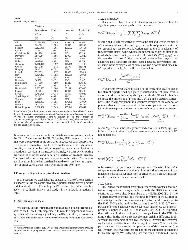
Table 1Dimensionality of the data.

Number of

Transactions Exporters Importers Relationships

sb(c)pt s b(c) sb(c)p

(1) (2) (3) (4)

All 37,796,239 70,649 1,103,275 8,626,857Austria 893,889 14,924 31,638 232,339Belgium 6,329,954 46,765 128,592 1,397,788Cyprus 63,891 3061 2271 19,906Czech Republic 261,788 8601 8101 50,723Denmark 697,829 15,106 17,968 159,829Estonia 53,873 2283 1617 12,498Finland 404,946 9287 9978 83,978Germany 6,661,428 40,437 228,985 1,414,047Greece 825,919 13,514 25,577 235,831Hungary 203,617 6873 5884 40,803Ireland 532,835 11,297 12,898 138,614Italy 5,134,450 34,992 188,556 1,290,050Latvia 53,164 2546 1796 14,281Lithuania 60,250 3420 2342 16,187Luxembourg 941,590 19,289 18,226 254,588Malta 44,014 2395 1279 12,454Netherlands 2,286,535 28,684 63,231 506,606Poland 431,354 11,956 16,664 95,659Portugal 1,717,826 20,974 42,307 394,948Slovak Republic 79,645 4008 2913 18,491Slovenia 110,763 3548 2760 20,896Spain 5,355,890 36,395 164,399 1,230,907Sweden 767,925 13,547 19,947 156,392United Kingdom 3,882,864 32,049 105,346 829,042

Notes: Column (1) is the number of transactions recorded over 2002–2006. Columns(2) and (3), respectively, report the number of French exporters and European importersinvolved in these transactions. Finally, column (4) is the number ofexporter×importer×product triplets. The ratio of column (4) to (1) allows us to recoverthemeannumber of transactions observed over time for a particularfirm-to-firm relation-ship and a particular product.

5F. Fontaine et al. / Journal of International Economics 124 (2020) 103300

this reason, we compute a number of statistics on a sample restricted tothe 15 “old” members of the EU.15 Likewise, EMU members are thosethat were already part of the euro-area in 2002. For each observation,we observe a transaction-specific price quote. We use the high dimen-sionality to condition the statistics regarding the variance of prices ona particular position in the network. Namely, we start by computingthe variance of prices conditional on a particular product×quarter.Then,we further focus on price discrepancieswithin a firm. The remain-ing dimensions in the data can then be used to discuss how the disper-sion of prices varies across firms, over space, and over time.

3. From price dispersion to price discrimination

In this section, we establish that a substantial share of the dispersionin export prices in the data is driven by exporters selling a given productat different prices to different buyers. We call such individual price be-havior “price discrimination” and study it in more details in sections 4and 5.

3.1. Price dispersion in the EU

We start by documenting that the product-level prices of French ex-ports to the EU are highly dispersed. A third of this dispersion is drivenby individual sellers charging their buyers different prices, whereas twothirds of thedispersion is attributable to average price differences acrosssellers.

15 When working on the later 2012–2016 period, we also neglect transactions involvingimporters in Romania, Bulgaria, and Croatia because these countries joined the EU onlyrecently.

3.1.1. MethodologyHereafter, the object of interest is the dispersion of prices,within a 8-

digit level product category, which we measure as:

Var scb cð Þpt psb cð Þpt

� �¼ 1

Npt−1

Xs

Xc

Xb cð Þ

psb cð Þpt−pscb cð Þpt

� �2

where p and Var(p), respectively, refer to the first and second momentsof the cross-section of prices andNpt is the number of price quotes in thecorresponding cross-section. Subscripts refer to the dimensionality ofthe corresponding variable, whereas superscripts denote the dimensioninwhich the correspondingmoment is calculated. Varptscb(c)(psb(c)pt) thusdenotes the variance of prices computed across sellers, buyers, andcountries, for a particular product×period. Because the variance is in-creasing in the average level of prices, we use a normalized measureof dispersion, namely, the coefficient of variation:

CVscb cð Þpt psb cð Þpt

� �¼

ffiffiffiffiffiffiffiffiffiffiffiffiffiffiffiffiffiffiffiffiffiffiffiffiffiffiffiffiffiffiffiffiffiffiffiffiVarscb cð Þ

pt psb cð Þpt� �r

pscb cð Þpt

In examining what share of these price discrepancies is attributableto different exporters selling a given product at different prices versusexporters price discriminating their partners in the EU, we further de-compose the dispersion of prices into a within and a between compo-nents. The within component is a weighted average of the variance ofprices within an exporter s, and the between component measures var-iations in mean prices between exporters of the same good. Formally,

Varscb cð Þpt psb cð Þpt

� �¼

Xs

Nspt−1Npt−1

Varb cð Þspt psb cð Þpt

� �|fflfflfflfflfflfflfflfflfflfflfflfflfflfflfflfflfflfflfflfflfflfflfflffl{zfflfflfflfflfflfflfflfflfflfflfflfflfflfflfflfflfflfflfflfflfflfflfflffl}

Within

þwVarspt pb cð Þspt

� �|fflfflfflfflfflfflfflfflfflfflffl{zfflfflfflfflfflfflfflfflfflfflffl}

Between

ð1Þ

where Nspt is the number of buyers connected to seller s, Varsptb(c)(psb(c)pt)is the variance of prices that this exporter sets on transactions with dif-ferent partners,

Varcb cð Þspt psb cð Þpt

� �¼ 1

Nspt−1

Xc

Xb cð Þ

psb cð Þpt−pcb cð Þspt

� �2

and

wVarspt pb cð Þspt

� �¼

Xs

Nspt−1Npt−1

pb cð Þspt −pscb cð Þ

pt

� �2

is the variance of exporter-specific average prices. The ratio of thewithincomponent over the overall variance of prices is thus a measure of howmuch the cross-sectional dispersion of prices within a product is attrib-utable to price discrepancies within a seller.

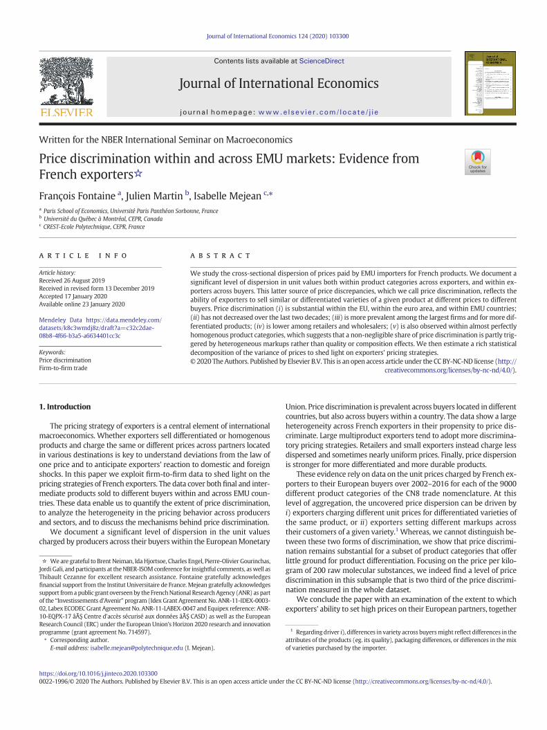
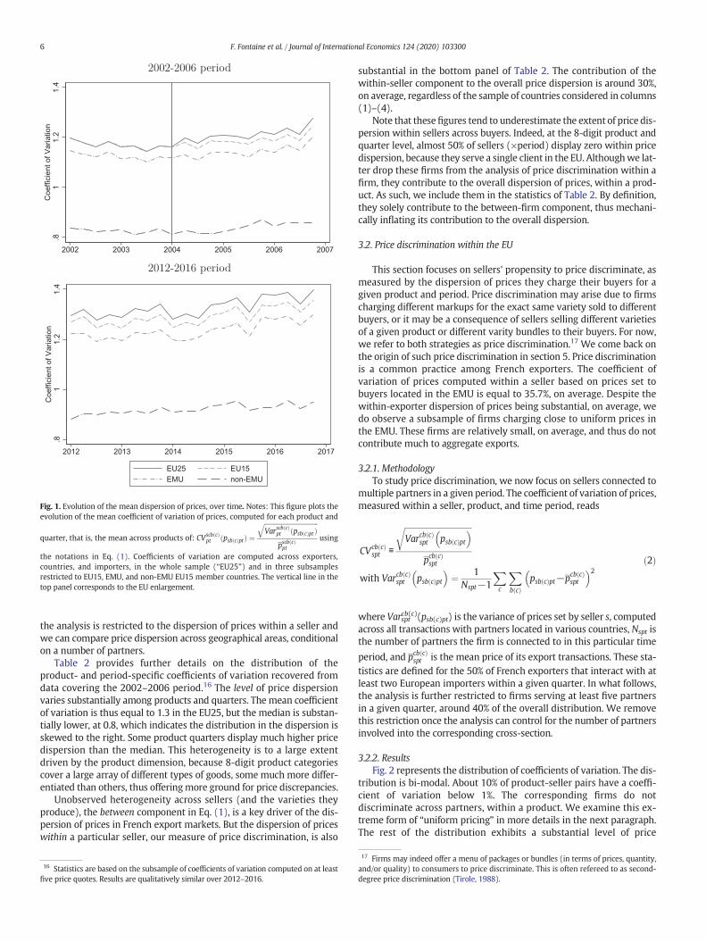
3.1.2. ResultsFig. 1 shows the evolution over time of the average coefficient of var-

iation, using various country samples, namely, the EU25, the subset ofcountries that were already members of the EU in 2002 (EU15), the11 original EMU countries, and the three members of the EU that donot participate in the common currency. The top panel corresponds tothe 2002–2006 period, and the bottom one is for 2012–2016. The dis-persion of prices is relatively stable over each subperiod, but price dis-persion is higher in 2012–2016 than over 2002–2006. As expected,the coefficient of price variations is, on average, lower in the EMU sub-sample than in the whole EU. But the most striking difference is ob-served in the subsample of non-EMUmembers, in which the recoveredcoefficient of variation is an order of magnitude lower. This result is inpart mechanical because this sample consists of three countries (theUK, Denmark and Sweden) that are not the most popular destinationsfor French exports. We further dig into this result in section 4.1, when

.81

1.2

1.4

Coe

ffici

ent o

f Var

iatio

n

2002 2003 2004 2005 2006 2007

.81

1.2

1.4

Coe

ffici

ent o

f Var

iatio

n

2012 2013 2014 2015 2016 2017

EU25 EU15EMU non-EMU

Fig. 1. Evolution of the mean dispersion of prices, over time. Notes: This figure plots theevolution of the mean coefficient of variation of prices, computed for each product and

quarter, that is, the mean across products of: CVscbðcÞpt ðpsbðcÞpt Þ ¼

ffiffiffiffiffiffiffiffiffiffiffiffiffiffiffiffiffiffiffiffiffiffiffiffiffiffiffiffiffiffiffiffiffiffiVarscbðcÞpt ðpsbðcÞpt Þ

qpscbðcÞpt

using

the notations in Eq. (1). Coefficients of variation are computed across exporters,countries, and importers, in the whole sample (“EU25”) and in three subsamplesrestricted to EU15, EMU, and non-EMU EU15 member countries. The vertical line in thetop panel corresponds to the EU enlargement.

6 F. Fontaine et al. / Journal of International Economics 124 (2020) 103300

the analysis is restricted to the dispersion of prices within a seller andwe can compare price dispersion across geographical areas, conditionalon a number of partners.

Table 2 provides further details on the distribution of theproduct- and period-specific coefficients of variation recovered fromdata covering the 2002–2006 period.16 The level of price dispersionvaries substantially among products and quarters. The mean coefficientof variation is thus equal to 1.3 in the EU25, but the median is substan-tially lower, at 0.8, which indicates the distribution in the dispersion isskewed to the right. Some product quarters display much higher pricedispersion than the median. This heterogeneity is to a large extentdriven by the product dimension, because 8-digit product categoriescover a large array of different types of goods, some much more differ-entiated than others, thus offeringmore ground for price discrepancies.

Unobserved heterogeneity across sellers (and the varieties theyproduce), the between component in Eq. (1), is a key driver of the dis-persion of prices in French export markets. But the dispersion of priceswithin a particular seller, our measure of price discrimination, is also

16 Statistics are based on the subsample of coefficients of variation computed on at leastfive price quotes. Results are qualitatively similar over 2012–2016.

substantial in the bottom panel of Table 2. The contribution of thewithin-seller component to the overall price dispersion is around 30%,on average, regardless of the sample of countries considered in columns(1)–(4).

Note that thesefigures tend to underestimate the extent of price dis-persion within sellers across buyers. Indeed, at the 8-digit product andquarter level, almost 50% of sellers (×period) display zero within pricedispersion, because they serve a single client in the EU. Althoughwe lat-ter drop these firms from the analysis of price discrimination within afirm, they contribute to the overall dispersion of prices, within a prod-uct. As such, we include them in the statistics of Table 2. By definition,they solely contribute to the between-firm component, thus mechani-cally inflating its contribution to the overall dispersion.

3.2. Price discrimination within the EU

This section focuses on sellers' propensity to price discriminate, asmeasured by the dispersion of prices they charge their buyers for agiven product and period. Price discrimination may arise due to firmscharging different markups for the exact same variety sold to differentbuyers, or it may be a consequence of sellers selling different varietiesof a given product or different varity bundles to their buyers. For now,we refer to both strategies as price discrimination.17 We come back onthe origin of such price discrimination in section 5. Price discriminationis a common practice among French exporters. The coefficient ofvariation of prices computed within a seller based on prices set tobuyers located in the EMU is equal to 35.7%, on average. Despite thewithin-exporter dispersion of prices being substantial, on average, wedo observe a subsample of firms charging close to uniform prices inthe EMU. These firms are relatively small, on average, and thus do notcontribute much to aggregate exports.

3.2.1. MethodologyTo study price discrimination, we now focus on sellers connected to

multiple partners in a given period. The coefficient of variation of prices,measured within a seller, product, and time period, reads

CVcb cð Þspt ≡

ffiffiffiffiffiffiffiffiffiffiffiffiffiffiffiffiffiffiffiffiffiffiffiffiffiffiffiffiffiffiffiffiffiffiVarcb cð Þ

spt psb cð Þpt� �r

pcb cð Þspt

with Varcb cð Þspt psb cð Þpt

� �¼ 1

Nspt−1

Xc

Xb cð Þ

psb cð Þpt−pcb cð Þspt

� �2ð2Þ

where Varsptcb(c)(psb(c)pt) is the variance of prices set by seller s, computedacross all transactions with partners located in various countries, Nspt isthe number of partners the firm is connected to in this particular time

period, and pcbðcÞspt is the mean price of its export transactions. These sta-tistics are defined for the 50% of French exporters that interact with atleast two European importers within a given quarter. In what follows,the analysis is further restricted to firms serving at least five partnersin a given quarter, around 40% of the overall distribution. We removethis restriction once the analysis can control for the number of partnersinvolved into the corresponding cross-section.

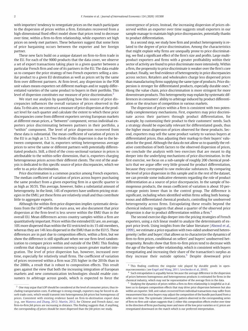
3.2.2. ResultsFig. 2 represents the distribution of coefficients of variation. The dis-

tribution is bi-modal. About 10% of product-seller pairs have a coeffi-cient of variation below 1%. The corresponding firms do notdiscriminate across partners, within a product. We examine this ex-treme form of “uniform pricing” in more details in the next paragraph.The rest of the distribution exhibits a substantial level of price

17 Firms may indeed offer a menu of packages or bundles (in terms of prices, quantity,and/or quality) to consumers to price discriminate. This is often refereed to as second-degree price discrimination (Tirole, 1988).

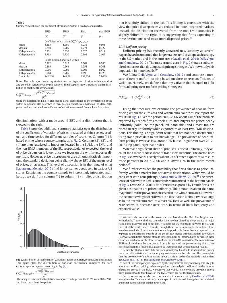
Table 2Summary statistics on the coefficient of variation, within a product, and quarter.

EU25 EU15 EMU non-EMU

(1) (2) (3) (4)

Coefficient of variation CVptscb(c)(psb(c)pt)

Mean 1.293 1.280 1.236 0.998Median 0.790 0.785 0.774 0.72210th percentile 0.331 0.330 0.325 0.31290th percentile 2.753 2.720 2.595 2.007

Contribution dispersion within sMean 0.312 0.312 0.304 0.286Median 0.265 0.264 0.253 0.20310th percentile 0.006 0.006 0.005 0.00290th percentile 0.704 0.705 0.696 0.725Count obs 142,266 141,521 138,354 75,669

Notes: The table reports summary statistics on the dispersion of prices within a productand period, in various country sub-samples. The first panel reports statistics on the distri-bution of coefficients of variations:

CVscbðcÞpt ðpsbðcÞpt Þ ¼

ffiffiffiffiffiffiffiffiffiffiffiffiffiffiffiffiffiffiffiffiffiffiffiffiffiffiffiffiffiffiffiffiffiffiVarscbðcÞpt ðpsbðcÞpt Þ

qpscbðcÞpt

using the notations in Eq. (1). The second panel corresponds to the contribution of thewithin component also described in this equation. Statistics are based on the 2002–2006period and are restricted to coefficients of variation recovered from at least five points.

7F. Fontaine et al. / Journal of International Economics 124 (2020) 103300

discrimination, with a mode around 25% and a distribution that isskewed to the right.

Table 3 provides additional summary statistics over the distributionof the coefficients of variation of prices, measured within a seller, prod-uct, and time period for different samples of countries. Column (1) isbased on the whole country sample, as is Fig. 2. Columns (2), (3), and(4) are then restricted to importers located in the EU15, the EMU, andthe non-EMU members of the EU, respectively. As expected, the levelof price dispersion is lower once we focus on the within-exporter di-mension. However, price discrepancies are still quantitatively impor-tant, the standard deviation being slightly above 35% of the mean levelof prices, on average. This level of dispersion is in the range of whatKaplan and Menzio (2015) find for consumer goods sold in various USstores. Restricting the country sample to increasingly integrated mar-kets as we do from column (1) to column (3) implies a distribution

02

46

810

Per

cent

0 .5 1 1.5 2Coefficient variation

Fig. 2. Distribution of coefficients of variations, across exporters, product and time. Notes:This figure plots the distribution of variation coefficients, computed for eachexporter×product×period according to Eq. (2):

CVcbðcÞspt ðpsbðcÞptÞ ¼

ffiffiffiffiffiffiffiffiffiffiffiffiffiffiffiffiffiffiffiffiffiffiffiffiffiffiffiffiffiffiffiffiffiVarcbðcÞspt ðpsbðcÞptÞ

qpcbðcÞspt

The analysis is restricted to statistics computed on buyers in the EU25, over 2002–2006and based on at least five points.

that is slightly shifted to the left. This finding is consistent with theview that price discrepancies are reduced in more integrated markets.Instead, the distribution recovered from the non-EMU countries isslightly shifted to the right, thus suggesting that firms exporting tothese destinations tend to set more dispersed prices.18

3.2.3. Uniform pricingUniform pricing has recently attracted new scrutiny as several

papers have documented that large retailers tend to adopt such strategyin the US market, and in the euro area (Cavallo et al., 2014; DellaVignaand Gentzkow, 2017). The mass around zero in Fig. 2 shows a subsam-ple of exporters that do adopt suchpricing strategies.Wenow study thispopulation in more details.19

We follow DellaVigna and Gentzkow (2017) and compute a mea-sure of nearly uniform pricing based on close to zero coefficients ofvariation. Namely, we define a dummy variable that is equal to 1 forfirms adopting near uniform pricing strategies:

NUPspt ¼ 1 CVcb cð Þspt b :01

h ið3Þ

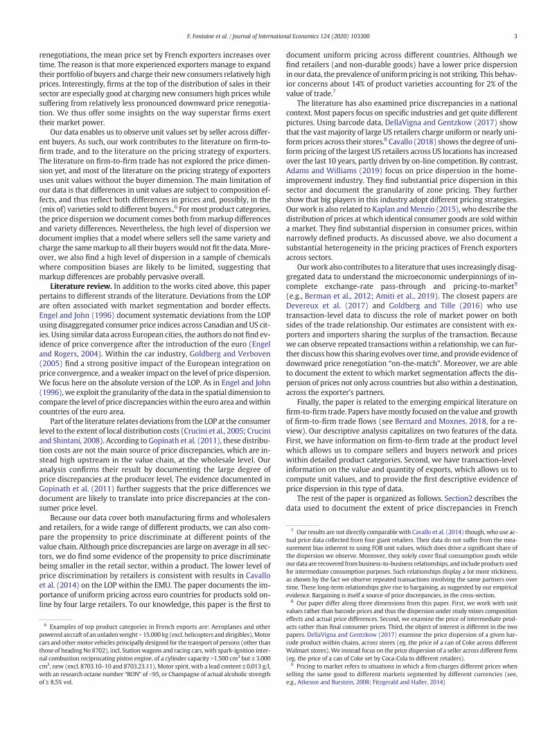
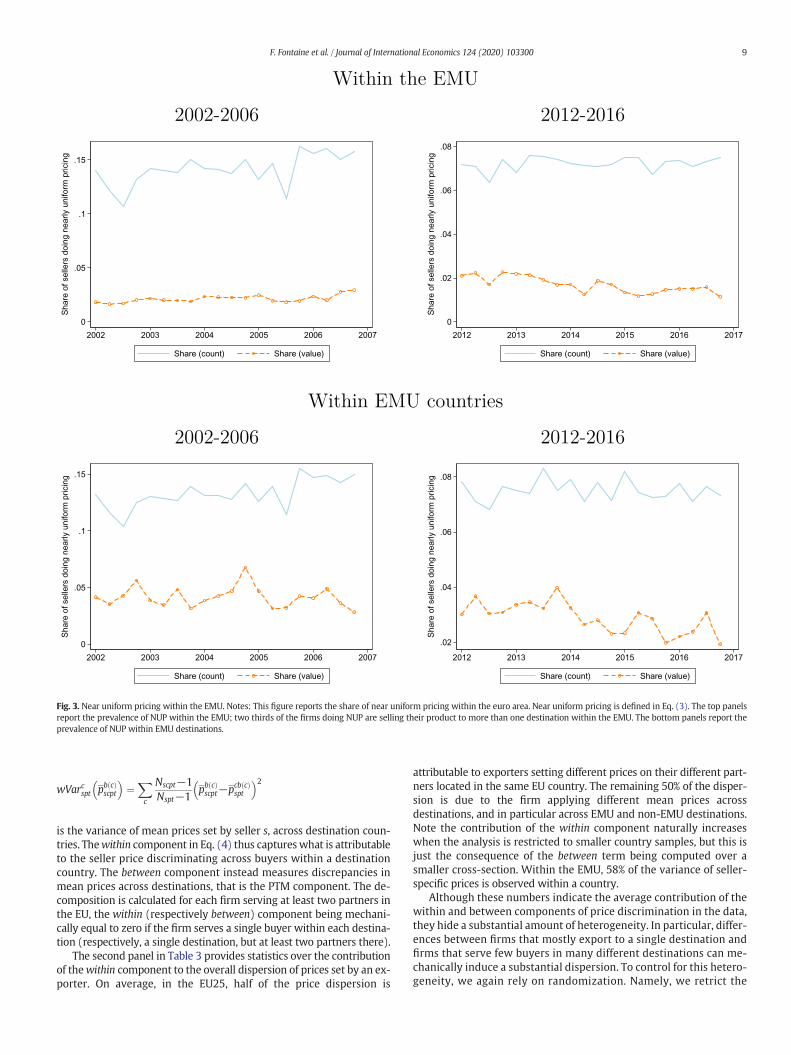
Using that measure, we examine the prevalence of near uniformpricing within the euro area and within euro countries. We report theresults in Fig. 3. Over the period 2002–2006, about 14% of the productsexported by French firms to their euro-area buyers are priced nearlyuniformly (solid line, top panel, left-hand side) and almost 10% arepriced nearly uniformly while exported to at least two EMU destina-tions. This finding is a significant result that has not been documentedusing trade-price data to our knowledge. The prevalence of near uni-form pricing is twice as low, around 7%, but still significant over 2012–2016 (top panel, right-hand side).

Whereas a significant share of products is priced uniformly, they ac-count for a more modest share of trade in value terms. The dotted linesin Fig. 3 show that NUPweights about 2% of French exports toward eurotrade partners in 2002–2006 and a lower 1.7% in the more recentperiod.20

We further consider the possibility that firms choose to price uni-formly within a market but not across destinations, which would beconsistent with zone pricing (Adams andWilliams, 2019).21 The preva-lence of NUPwithin EMU countries is summarized in the bottom panelsof Fig. 3. Over 2002–2006, 13% of varieties exported by French firms in agiven destination are priced uniformly. This amount is about the samemagnitude as the prevalence observed in thewhole euro area. However,the economicweight of NUPwithin a destination is about twice as largeas in the overall euro area, at almost 4%. Here as well, the prevalence ofNUP seems to decrease over time, in terms of both frequency andexported value.

18 We have also computed the same statistics based on the EMU less Belgium andNetherlands. Trade with these countries is somewhat biased by the presence of majortrade ports in Anvers and Rotterdam. A substantial share of trade between the EU andthe rest of the world indeed transits through these ports. In principle, these trade flowshave been excluded from the dataset as we dropped trade flows that are reported to beexported to destinations outside of the EU but exit France through another EU country.However, a significant number of tradeflows could still be intermediated byfirms in thesecountries, inwhich case theflow is recorded as an intra-EU transaction. The comparison ofEMU results with numbers recovered from this restricted sample were very similar. Weconcluded from this finding that exports to these countries do not bias our results.19 Remember that our price data are not especially well-suited to study uniform pricingsince the differentiation of the underlying varieties cannot be ruled out. This can explainthat the prevalence of uniform pricing in our data is an order of magnitude smaller thanin Cavallo et al. (2014) and DellaVigna and Gentzkow (2017).20 Part of the discrepancy is explained by the largest firms being relatively less likely toadopt near uniform pricing. When we perform the analysis conditional on the numberof partners served in the EMU, we observe that NUP is relatively more prevalent amongfirms serving two to four buyers in the EMU, which are not the largest ones.21 Such zone pricing has also been documented to some extent by Cavallo et al. (2014),who show that Zara has a pricing strategy specific to Spain and Portugal on the one hand,and other euro countries on the other hand.

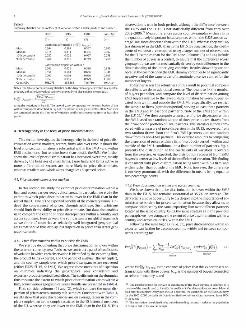
Table 3Summary statistics on the coefficient of variation, within a seller, product, and quarter.

EU25 EU15 EMU non-EMU

(1) (2) (3) (4)

Coefficient of variation CVsptcb(c)(psb(c)pt)

Mean 0.364 0.362 0.357 0.365Median 0.314 0.311 0.305 0.30710th percentile 0.027 0.026 0.027 0.05890th percentile 0.761 0.758 0.749 0.760

Contribution dispersion within cMean 0.506 0.526 0.580 0.839Median 0.551 0.581 0.656 0.94110th percentile 0.000 0.001 0.020 0.50590th percentile 0.950 0.957 0.979 1.000Count Obs 863,275 835,386 716,780 104,410

Notes: The table reports summary statistics on the dispersion of prices within an exporter,product, and period, in various country samples. Price dispersion is measured as:

CVcbðcÞspt ðpsbðcÞptÞ ¼

ffiffiffiffiffiffiffiffiffiffiffiffiffiffiffiffiffiffiffiffiffiffiffiffiffiffiffiffiffiffiffiffiffiVarcbðcÞspt ðpsbðcÞptÞ

qpcbðcÞspt

using the notations in Eq. (2). The second panel corresponds to the contribution of thewithin component described in Eq. (4). The period of analysis is 2002–2006. Statisticsare computed on the distribution of variation coefficients recovered from at least fivepoints.

22 One possible reason for the lack of significance of the EU25 dummy in column (1) isthe size of the sample used to identify the coefficient. Our dataset does not cover bilateraldata prior to countries' entry into the EU. Therefore, the coefficient on the EU25 dummyfor the 2002–2006 period is de facto identified over observations recovered from 2004to 2006 data.23 This restriction reveals itself to be quite demanding, because it reduces the populationof firms to 34% of the overall sample.

8 F. Fontaine et al. / Journal of International Economics 124 (2020) 103300

4. Heterogeneity in the level of price discrimination

This section investigates the heterogeneity in the level of price dis-crimination across markets, sectors, firms, and over time. It shows thelevel of price discrimination is substantial within the EMU - and withinEMUdestinations - but remains lower than outside the EMU.We furthershow the level of price discrimination has increased over time, mostlydriven by the behavior of small firms. Large firms and firms active inmore differentiated sectors are more likely to price discriminate,whereas retailers and wholesalers charge less dispersed prices.

4.1. Price discrimination across markets

In this section, we study the extent of price discrimination within afirm and across various geographical areas. In particular, we study theextent to which price discrimination is lower in the EMU than in therest of the EU. One of the expected benefits of themonetary union is in-deed the convergence of prices, through arbitrage. Such arbitrageshould limit firms' ability to price discriminate. Our data also enablesus to compare the extent of price discrepancies within a country andacross countries. Here as well, the comparison is insightful inasmuchas we think of countries as relatively well-integrated geographicalareas that should thus display less dispersion in prices than larger geo-graphical units.

4.1.1. Price discrimination within vs outside the EMUWe start by documenting that price discrimination is lower within

the common currency area. To do so, we construct a panel of coefficientsof variation inwhich each observation is identified by the exportingfirm,the product being exported, and the period of analysis (the spt triplet),and the country sample over which price discrepancies are recovered(either EU25, EU15, or EMU). We regress these measures of dispersionon dummies indicating the geographical area considered andexporter×product×period fixed effects. The coefficients on the dummiesthus measure the extent to which price discrimination varies within afirm, across various geographical areas. Results are presented in Table 4.

First, consider columns (1) and (2), which compare the mean dis-persion of prices across country sub-samples. Consistent with Table 3,results show that price discrepancies are, on average, larger in the com-plete sample than in the sample restricted to the 15 historical membersof the EU, whereas they are lower in the EMU than in the EU15. This

observation is true in both periods, although the difference betweenthe EU25 and the EU15 is not statistically different from zero over2002–2006.22 Mean differences across country samples within a firmare quantitatively important because prices within the EU25 are, on av-erage, 10% more dispersed than within the EU15, whereas they are 14%less dispersed in the EMU than in the EU15. By construction, the coeffi-cients of variation are computed using a larger number of observationsfor the EU samples than for the EMU one. Columns (3) and (4) includethe number of buyers as a control, to ensure that the differences acrossgeographic areas are not mechanically driven by such differences in thedimensionality of the underlying variables. Results show they are notbecause the coefficient on the EMUdummy continues to be significantlynegative and of the same order of magnitude once we control for thenumber of buyers.

To further assess the robustness of this result to potential composi-tion effects, we do an additional exercise. The idea is to fix the numberof buyers per seller, and compare the level of discrimination amongEMU buyers relative to the level of discrimination between buyers lo-cated both within and outside the EMU. More specifically, we restrictthe sample to firms (×product×period) serving at least three partnersin the EMU and at least one partner outside of the EMU (but withinthe EU15).23 We then compute a measure of price dispersion withinthe EMU based on a random sample of three price quotes, drawn fromthe firm-specific portfolio of EMU partners. This statistics is then com-pared with a measure of price dispersion in the EU15, recovered fromtwo random draws from the firm's EMU partners and one randomdraw from its non-EMU partners. This exercise amounts to comparingthe dispersion of prices within a firm (×product×period), within andoutside of the EMU, conditional on a fixed number of partners. Fig. 4presents the distribution of the coefficients of variation recoveredfrom the exercise. As expected, the distribution recovered from EMUbuyers is denser at low levels of the coefficient of variation. This findingis consistent with price discrimination being lower within a firm, andwithin rather than outside of the EMU. Note, however, the differenceis not very pronounced, with the difference in means being equal totwo percentage points.

4.1.2. Price discrimination within and across countriesWe have shown that price discrimination is lower within the EMU

than in the EU15, but remains substantial at 35.7%, on average. Thedata offer a unique opportunity to dig deeper into the importance of ad-ministrative borders for price discrimination because they allow us tocompare prices set by the same exporting firm over different partnerslocated in the same country. Using the same strategy as in the previousparagraph, we now compare the extent of price discrimination within acountry and across countries, within the EMU.

Following the same logic as in Eq. (1), price discrepancies within anexporter can further be decomposed into within and between compo-nents according to:

Varcb cð Þspt psb cð Þpt

� �¼

Xc

Nscpt−1Nspt−1

Varb cð Þscpt psb cð Þpt

� �|fflfflfflfflfflfflfflfflfflfflfflfflfflfflfflfflfflfflfflfflfflfflfflfflffl{zfflfflfflfflfflfflfflfflfflfflfflfflfflfflfflfflfflfflfflfflfflfflfflfflffl}

Within

þwVarcspt pb cð Þscpt

� �|fflfflfflfflfflfflfflfflfflfflffl{zfflfflfflfflfflfflfflfflfflfflffl}

Between

ð4Þ

where Varscptb(c)(psb(c)pt) is the variance of prices that this exporter sets ontransactions with these buyers, Nscpt is the number of buyers connectedto seller s in country c, and

0

.05

.1

.15

Sha

re o

f sel

lers

doi

ng n

early

uni

form

pric

ing

2002 2003 2004 2005 2006 2007

Share (count) Share (value)

0

.02

.04

.06

.08

Sha

re o

f sel

lers

doi

ng n

early

uni

form

pric

ing

2012 2013 2014 2015 2016 2017

Share (count) Share (value)

0

.05

.1

.15

Sha

re o

f sel

lers

doi

ng n

early

uni

form

pric

ing

2002 2003 2004 2005 2006 2007

Share (count) Share (value)

.02

.04

.06

.08

Sha

re o

f sel

lers

doi

ng n

early

uni

form

pric

ing

2012 2013 2014 2015 2016 2017

Share (count) Share (value)

Fig. 3. Near uniform pricing within the EMU. Notes: This figure reports the share of near uniform pricing within the euro area. Near uniform pricing is defined in Eq. (3). The top panelsreport the prevalence of NUP within the EMU; two thirds of the firms doing NUP are selling their product to more than one destination within the EMU. The bottom panels report theprevalence of NUP within EMU destinations.

9F. Fontaine et al. / Journal of International Economics 124 (2020) 103300

wVarcspt pb cð Þscpt

� �¼

Xc

Nscpt−1Nspt−1

pb cð Þscpt−pcb cð Þ

spt

� �2

is the variance of mean prices set by seller s, across destination coun-tries. Thewithin component in Eq. (4) thus captureswhat is attributableto the seller price discriminating across buyers within a destinationcountry. The between component instead measures discrepancies inmean prices across destinations, that is the PTM component. The de-composition is calculated for each firm serving at least two partners inthe EU, the within (respectively between) component being mechani-cally equal to zero if the firm serves a single buyer within each destina-tion (respectively, a single destination, but at least two partners there).

The second panel in Table 3 provides statistics over the contributionof thewithin component to the overall dispersion of prices set by an ex-porter. On average, in the EU25, half of the price dispersion is

attributable to exporters setting different prices on their different part-ners located in the same EU country. The remaining 50% of the disper-sion is due to the firm applying different mean prices acrossdestinations, and in particular across EMU and non-EMU destinations.Note the contribution of the within component naturally increaseswhen the analysis is restricted to smaller country samples, but this isjust the consequence of the between term being computed over asmaller cross-section. Within the EMU, 58% of the variance of seller-specific prices is observed within a country.

Although these numbers indicate the average contribution of thewithin and between components of price discrimination in the data,they hide a substantial amount of heterogeneity. In particular, differ-ences between firms that mostly export to a single destination andfirms that serve few buyers in many different destinations can me-chanically induce a substantial dispersion. To control for this hetero-geneity, we again rely on randomization. Namely, we retrict the

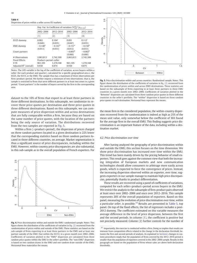
Table 4Dispersion of prices within a seller across EU markets.

Dep. Var: ln Coefficient of variation CVszptcb(c)(psb(c)pt)

2002–2006 2012–2016 2002–2006 2012–2016

(1) (2) (3) (4)

EU25 dummy 0.082 0.104c 0.091 0.112c

(0.049) (0.035) (0.047) (0.035)EMU dummy −0.140a −0.141b −0.151a −0.150b

(0.013) (0.033) (0.012) (0.033)Count partners −0.003b −0.002b

(0.000) (0.000)# Observations 2,063,813 2,742,399 2,063,813 2,742,399Fixed Effects Product×period×seller# FE 961,105 1,270,168 961,105 1,270,168Adjusted R2 (overall) 0.930 0.874 0.930 0.875

Notes: The LHS variable is the log of the coefficient of variation, across buyers within aseller (for each product and quarter), calculated for a specific geographical area z, theEU25, the EU15, or the EMU. The sample thus has a maximum of three observations perfirm×product×period. We further impose a minimum of two observations; that is, thesample is restricted to firms that serve different partners in at least two zones in a givenperiod. “Count partners” is the number of buyers served by the firm in the correspondingarea.

0.5

11.

52

2.5

Den

sity

0 .5 1 1.5CV

Between Within

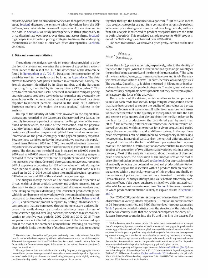
Fig. 5. Price discrimination within and across countries: Randomized sample. Notes: Thisfigure shows the distribution of the coefficients of variation in Eq. (2) recovered fromthe randomization of prices within and across EMU destinations. These statistics arebased on the subsample of firms exporting to at least three partners in three EMUcountries in a given month over 2002–2006. Coefficients of variation plotted in the“Between” dispersion are calculated from three random price quotes in three differentcountries in the seller's portfolio. The “within” dispersion is based on three randomprice quotes in each destination. Horizontal lines represent the means.

10 F. Fontaine et al. / Journal of International Economics 124 (2020) 103300

dataset to the 10% of firms that export to at least three partners inthree different destinations. In this subsample, we randomize to re-cover three price quotes per destination and three price quotes inthree different destinations. Based on this subsample, we can com-pute measures of price dispersion within and across destinationsthat are fully comparable within a firm, because they are based onthe same number of price quotes, with the location of the partnersbeing the only source of variation. The distributions recoveredfrom the two samples are reported in Fig. 5.

Within a firm (×product×period), the dispersion of prices chargedon three random partners located in a given destination is 22% lowerthat the corresponding statistics based on three random partners lo-cated in three different countries, on average. Market segmentation isthus a significant source of price discrepancies, including within theEMU. However, within-country price discrepancies are also substantial,in this sub-sample as in the overall population of French exporters. For

0.5

11.

52

2.5

Den

sity

0 .5 1 1.5CV

EMU Non-EMU

Fig. 4. Price discrimination within and outside the EMU: randomized sample. Notes: Thisfigure shows the distribution of the coefficients of variation in Eq. (2) recovered from therandomization of prices within and outside of the EMU. These statistics are based on thesub-sample of firms exporting to at least three partners in the EMU and at least onepartner outside of the EMU (but within the EU15) in a given month over 2002–2006.Coefficients of variation plotted in the “EMU” dispersion are calculated from threerandom price quotes within the EMU in the seller's portfolio. The “non-EMU” dispersionis based on two random draws in the EMU and one random draw outside of the EMU.Horizontal lines materialize the means.

themean firm in the considered population, the within-country disper-sion recovered from the randomization is indeed as high as 25% of themean unit value, only somewhat below the coefficient of 36% foundfor the average firm in the overall EMU. This finding suggests price dis-crimination is an important feature of the data, including within a des-tination market.

4.2. Price discrimination over time

After having analyzed the geography of price discrimination withinand outside the EMU, this section focuses on the time dimension. Weshow price discrimination has increased over time within the EMU.This trend has been mainly driven by the pricing behavior of small ex-porters. This result goes against the common view that both the increas-ing integration of European markets and new communicationtechnologies should allow consumers to arbitrage more easily acrossgoods, which is expected to force the convergence of prices. Instead,the increasing dispersion observed within an exporter, over time, sug-gests exporters in our samplemanage tomaintain high price discrepan-cies, potentially thanks to product differentiation.

These results are recovered using a panel of coefficients of variations,computed for each seller×product×period across buyers in the EMU.We restrict the analysis to the subsample offirm-product pairs observedat least once over 2002–2006 and once over 2012–2016. This samplerepresents 20% of the overall population of exporters. Based on thispanel, measuring the evolution of price discrimination over time,withina particular seller, is possible.24 Results are presented in Table 5, toppanel. On top of the fixed effects, the list of regressors includes a post-2012 dummy. The coefficient estimated on this variable measures theaverage difference in the level of price dispersion, between the firstand the second periods. In column (1), the coefficient is positive butnot precisely measured. Column (2) further controls for the number of

24 Importantly, the exercise is conducted within a firm. Doing so implies that results areimmune from composition effects related to the change in the declaration threshold, be-tween the first and second periods of analysis. As explained in Section2, changes in cus-toms procedures imply that the population of firms covered by the 2012–2016 period issmaller than the population of exporters covered in the 2002–2006 sample. Results in thisparagraph are based on the population of firms whose sales are above both declarationthresholds.

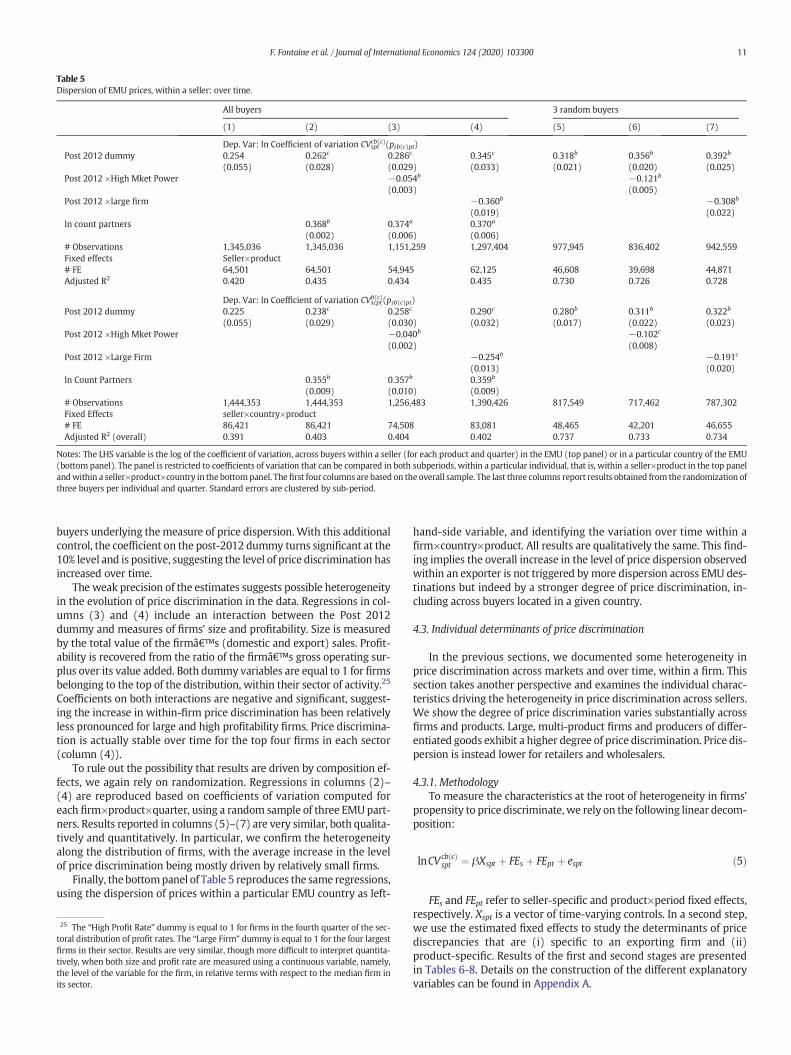
Table 5Dispersion of EMU prices, within a seller: over time.

All buyers 3 random buyers

(1) (2) (3) (4) (5) (6) (7)

Dep. Var: ln Coefficient of variation CVsptcb(c)(psb(c)pt)

Post 2012 dummy 0.254 0.262c 0.286c 0.345c 0.318b 0.356b 0.392b

(0.055) (0.028) (0.029) (0.033) (0.021) (0.020) (0.025)Post 2012 ×High Mket Power −0.054b −0.121b

(0.003) (0.005)Post 2012 ×large firm −0.360b −0.308b

(0.019) (0.022)ln count partners 0.368b 0.374a 0.370a

(0.002) (0.006) (0.006)# Observations 1,345,036 1,345,036 1,151,259 1,297,404 977,945 836,402 942,559Fixed effects Seller×product# FE 64,501 64,501 54,945 62,125 46,608 39,698 44,871Adjusted R2 0.420 0.435 0.434 0.435 0.730 0.726 0.728

Dep. Var: ln Coefficient of variation CVscptb(c)(psb(c)pt)

Post 2012 dummy 0.225 0.238c 0.258c 0.290c 0.280b 0.311b 0.322b

(0.055) (0.029) (0.030) (0.032) (0.017) (0.022) (0.023)Post 2012 ×High Mket Power −0.040b −0.102c

(0.002) (0.008)Post 2012 ×Large Firm −0.254b −0.191c

(0.013) (0.020)ln Count Partners 0.355b 0.357b 0.359b

(0.009) (0.010) (0.009)# Observations 1,444,353 1,444,353 1,256,483 1,390,426 817,549 717,462 787,302Fixed Effects seller×country×product# FE 86,421 86,421 74,508 83,081 48,465 42,201 46,655Adjusted R2 (overall) 0.391 0.403 0.404 0.402 0.737 0.733 0.734

Notes: The LHS variable is the log of the coefficient of variation, across buyers within a seller (for each product and quarter) in the EMU (top panel) or in a particular country of the EMU(bottom panel). The panel is restricted to coefficients of variation that can be compared in both subperiods, within a particular individual, that is, within a seller×product in the top panelandwithin a seller×product×country in the bottompanel. The first four columns are based on the overall sample. The last three columns report results obtained from the randomization ofthree buyers per individual and quarter. Standard errors are clustered by sub-period.

11F. Fontaine et al. / Journal of International Economics 124 (2020) 103300

buyers underlying themeasure of price dispersion.With this additionalcontrol, the coefficient on the post-2012 dummy turns significant at the10% level and is positive, suggesting the level of price discrimination hasincreased over time.

The weak precision of the estimates suggests possible heterogeneityin the evolution of price discrimination in the data. Regressions in col-umns (3) and (4) include an interaction between the Post 2012dummy and measures of firms' size and profitability. Size is measuredby the total value of the firm’s (domestic and export) sales. Profit-ability is recovered from the ratio of the firm’s gross operating sur-plus over its value added. Both dummy variables are equal to 1 for firmsbelonging to the top of the distribution, within their sector of activity.25

Coefficients on both interactions are negative and significant, suggest-ing the increase in within-firm price discrimination has been relativelyless pronounced for large and high profitability firms. Price discrimina-tion is actually stable over time for the top four firms in each sector(column (4)).

To rule out the possibility that results are driven by composition ef-fects, we again rely on randomization. Regressions in columns (2)–(4) are reproduced based on coefficients of variation computed foreach firm×product×quarter, using a random sample of three EMUpart-ners. Results reported in columns (5)–(7) are very similar, both qualita-tively and quantitatively. In particular, we confirm the heterogeneityalong the distribution of firms, with the average increase in the levelof price discrimination being mostly driven by relatively small firms.

Finally, the bottompanel of Table 5 reproduces the same regressions,using the dispersion of prices within a particular EMU country as left-

25 The “High Profit Rate” dummy is equal to 1 for firms in the fourth quarter of the sec-toral distribution of profit rates. The “Large Firm” dummy is equal to 1 for the four largestfirms in their sector. Results are very similar, though more difficult to interpret quantita-tively, when both size and profit rate are measured using a continuous variable, namely,the level of the variable for the firm, in relative terms with respect to the median firm inits sector.

hand-side variable, and identifying the variation over time within afirm×country×product. All results are qualitatively the same. This find-ing implies the overall increase in the level of price dispersion observedwithin an exporter is not triggered by more dispersion across EMU des-tinations but indeed by a stronger degree of price discrimination, in-cluding across buyers located in a given country.

4.3. Individual determinants of price discrimination

In the previous sections, we documented some heterogeneity inprice discrimination across markets and over time, within a firm. Thissection takes another perspective and examines the individual charac-teristics driving the heterogeneity in price discrimination across sellers.We show the degree of price discrimination varies substantially acrossfirms and products. Large, multi-product firms and producers of differ-entiated goods exhibit a higher degree of price discrimination. Price dis-persion is instead lower for retailers and wholesalers.

4.3.1. MethodologyTo measure the characteristics at the root of heterogeneity in firms'

propensity to price discriminate, we rely on the following linear decom-position:

lnCVcb cð Þspt ¼ βXspt þ FEs þ FEpt þ espt ð5Þ

FEs and FEpt refer to seller-specific and product×period fixed effects,respectively. Xspt is a vector of time-varying controls. In a second step,we use the estimated fixed effects to study the determinants of pricediscrepancies that are (i) specific to an exporting firm and (ii)product-specific. Results of the first and second stages are presentedin Tables 6-8. Details on the construction of the different explanatoryvariables can be found in Appendix A.

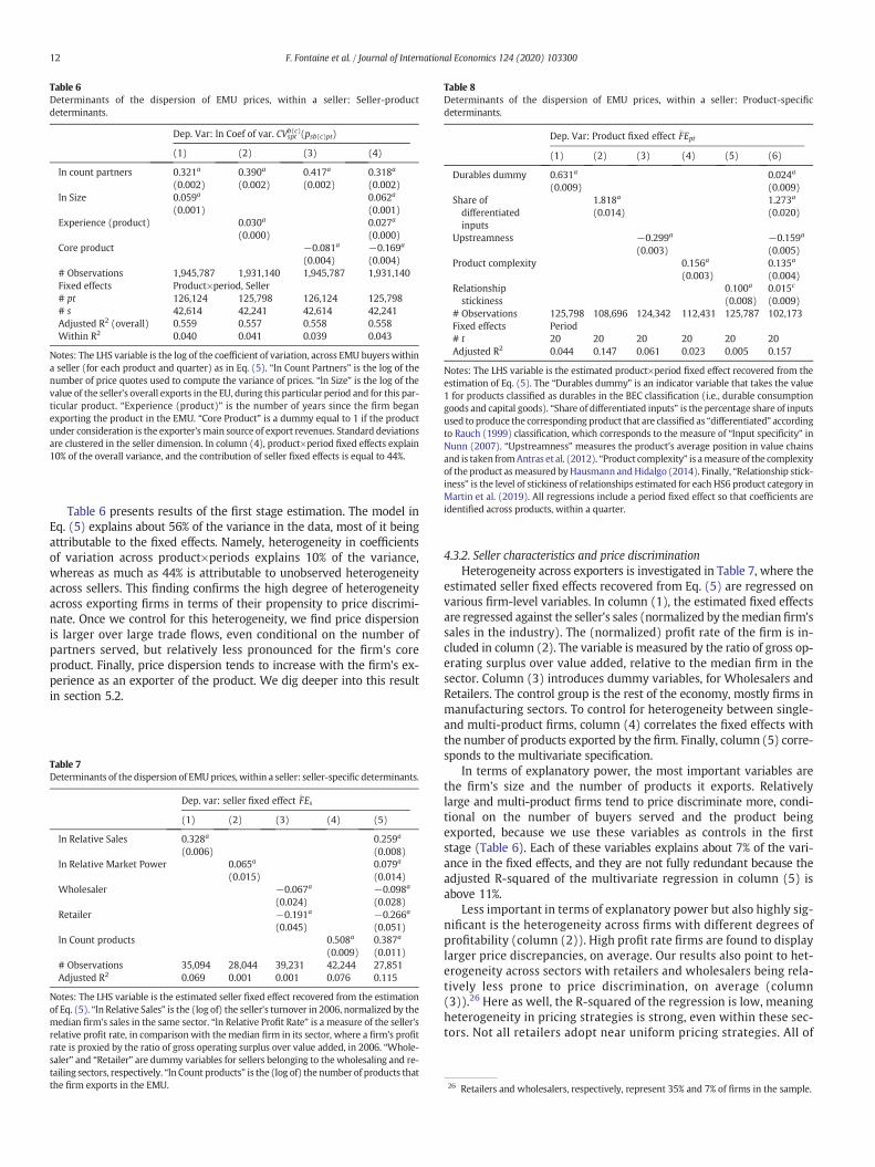
Table 6Determinants of the dispersion of EMU prices, within a seller: Seller-productdeterminants.

Dep. Var: ln Coef of var. CVsptb(c)(psb(c)pt)

(1) (2) (3) (4)

ln count partners 0.321a 0.390a 0.417a 0.318a

(0.002) (0.002) (0.002) (0.002)ln Size 0.059a 0.062a

(0.001) (0.001)Experience (product) 0.030a 0.027a

(0.000) (0.000)Core product −0.081a −0.169a

(0.004) (0.004)# Observations 1,945,787 1,931,140 1,945,787 1,931,140Fixed effects Product×period, Seller# pt 126,124 125,798 126,124 125,798# s 42,614 42,241 42,614 42,241Adjusted R2 (overall) 0.559 0.557 0.558 0.558Within R2 0.040 0.041 0.039 0.043

Notes: The LHS variable is the log of the coefficient of variation, across EMU buyers withina seller (for each product and quarter) as in Eq. (5). “ln Count Partners” is the log of thenumber of price quotes used to compute the variance of prices. “ln Size” is the log of thevalue of the seller's overall exports in the EU, during this particular period and for this par-ticular product. “Experience (product)” is the number of years since the firm beganexporting the product in the EMU. “Core Product” is a dummy equal to 1 if the productunder consideration is the exporter's main source of export revenues. Standard deviationsare clustered in the seller dimension. In column (4), product×period fixed effects explain10% of the overall variance, and the contribution of seller fixed effects is equal to 44%.

Table 8Determinants of the dispersion of EMU prices, within a seller: Product-specificdeterminants.

Dep. Var: Product fixed effect F̂Ept

(1) (2) (3) (4) (5) (6)

Durables dummy 0.631a 0.024a

(0.009) (0.009)Share ofdifferentiatedinputs

1.818a 1.273a

(0.014) (0.020)

Upstreamness −0.299a −0.159a

(0.003) (0.005)Product complexity 0.156a 0.135a

(0.003) (0.004)Relationshipstickiness

0.100a 0.015c

(0.008) (0.009)# Observations 125,798 108,696 124,342 112,431 125,787 102,173Fixed effects Period# t 20 20 20 20 20 20Adjusted R2 0.044 0.147 0.061 0.023 0.005 0.157

Notes: The LHS variable is the estimated product×period fixed effect recovered from theestimation of Eq. (5). The “Durables dummy” is an indicator variable that takes the value1 for products classified as durables in the BEC classification (i.e., durable consumptiongoods and capital goods). “Share of differentiated inputs” is the percentage share of inputsused to produce the corresponding product that are classified as “differentiated” accordingto Rauch (1999) classification, which corresponds to the measure of “Input specificity” inNunn (2007). “Upstreamness” measures the product's average position in value chainsand is taken fromAntras et al. (2012). “Product complexity” is ameasure of the complexityof the product asmeasured byHausmann andHidalgo (2014). Finally, “Relationship stick-iness” is the level of stickiness of relationships estimated for each HS6 product category inMartin et al. (2019). All regressions include a period fixed effect so that coefficients areidentified across products, within a quarter.

12 F. Fontaine et al. / Journal of International Economics 124 (2020) 103300

Table 6 presents results of the first stage estimation. The model inEq. (5) explains about 56% of the variance in the data, most of it beingattributable to the fixed effects. Namely, heterogeneity in coefficientsof variation across product×periods explains 10% of the variance,whereas as much as 44% is attributable to unobserved heterogeneityacross sellers. This finding confirms the high degree of heterogeneityacross exporting firms in terms of their propensity to price discrimi-nate. Once we control for this heterogeneity, we find price dispersionis larger over large trade flows, even conditional on the number ofpartners served, but relatively less pronounced for the firm's coreproduct. Finally, price dispersion tends to increase with the firm's ex-perience as an exporter of the product. We dig deeper into this resultin section 5.2.

Table 7Determinants of the dispersion of EMUprices, within a seller: seller-specific determinants.

Dep. var: seller fixed effect F̂Es

(1) (2) (3) (4) (5)

ln Relative Sales 0.328a 0.259a

(0.006) (0.008)ln Relative Market Power 0.065a 0.079a

(0.015) (0.014)Wholesaler −0.067a −0.098a

(0.024) (0.028)Retailer −0.191a −0.266a

(0.045) (0.051)ln Count products 0.508a 0.387a

(0.009) (0.011)# Observations 35,094 28,044 39,231 42,244 27,851Adjusted R2 0.069 0.001 0.001 0.076 0.115

Notes: The LHS variable is the estimated seller fixed effect recovered from the estimationof Eq. (5). “ln Relative Sales” is the (log of) the seller's turnover in 2006, normalized by themedian firm's sales in the same sector. “ln Relative Profit Rate” is a measure of the seller'srelative profit rate, in comparison with the median firm in its sector, where a firm's profitrate is proxied by the ratio of gross operating surplus over value added, in 2006. “Whole-saler” and “Retailer” are dummy variables for sellers belonging to the wholesaling and re-tailing sectors, respectively. “ln Count products” is the (log of) the number of products thatthe firm exports in the EMU.

4.3.2. Seller characteristics and price discriminationHeterogeneity across exporters is investigated in Table 7, where the

estimated seller fixed effects recovered from Eq. (5) are regressed onvarious firm-level variables. In column (1), the estimated fixed effectsare regressed against the seller's sales (normalized by themedian firm'ssales in the industry). The (normalized) profit rate of the firm is in-cluded in column (2). The variable is measured by the ratio of gross op-erating surplus over value added, relative to the median firm in thesector. Column (3) introduces dummy variables, for Wholesalers andRetailers. The control group is the rest of the economy, mostly firms inmanufacturing sectors. To control for heterogeneity between single-and multi-product firms, column (4) correlates the fixed effects withthe number of products exported by the firm. Finally, column (5) corre-sponds to the multivariate specification.

In terms of explanatory power, the most important variables arethe firm's size and the number of products it exports. Relativelylarge and multi-product firms tend to price discriminate more, condi-tional on the number of buyers served and the product beingexported, because we use these variables as controls in the firststage (Table 6). Each of these variables explains about 7% of the vari-ance in the fixed effects, and they are not fully redundant because theadjusted R-squared of the multivariate regression in column (5) isabove 11%.

Less important in terms of explanatory power but also highly sig-nificant is the heterogeneity across firms with different degrees ofprofitability (column (2)). High profit rate firms are found to displaylarger price discrepancies, on average. Our results also point to het-erogeneity across sectors with retailers and wholesalers being rela-tively less prone to price discrimination, on average (column(3)).26 Here as well, the R-squared of the regression is low, meaningheterogeneity in pricing strategies is strong, even within these sec-tors. Not all retailers adopt near uniform pricing strategies. All of

26 Retailers and wholesalers, respectively, represent 35% and 7% of firms in the sample.

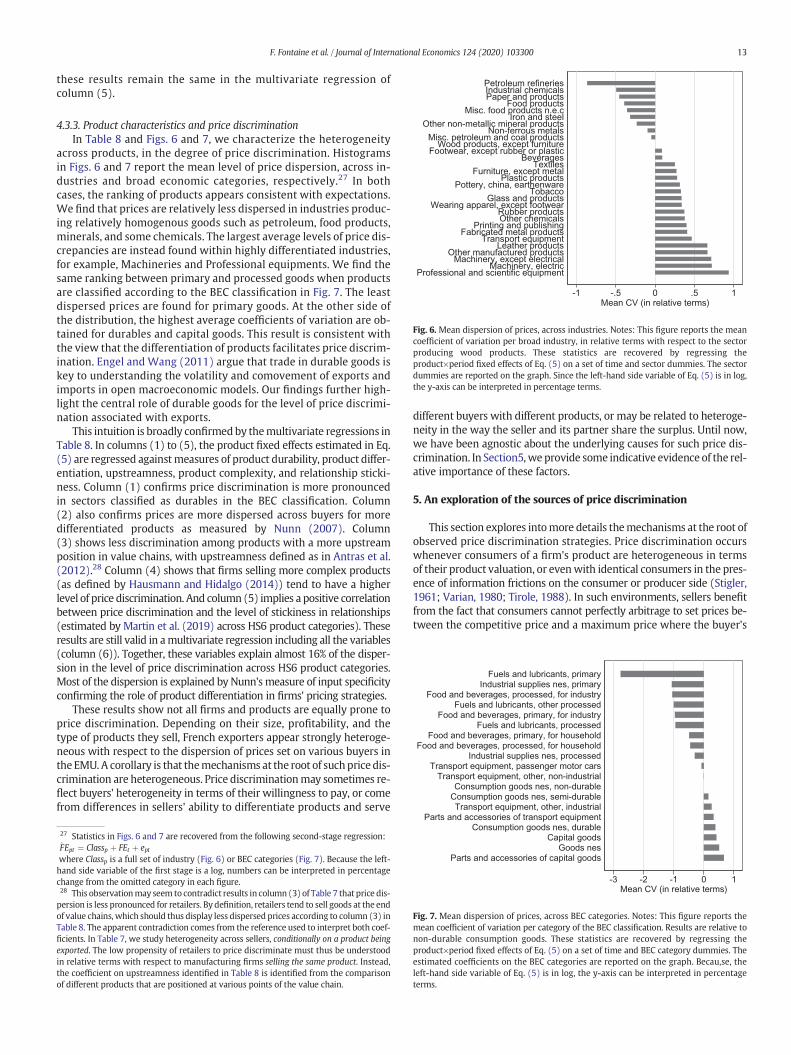
-1 -.5 0 .5 1Mean CV (in relative terms)

Professional and scientific equipmentMachinery, electric

Machinery, except electricalOther manufactured products

Leather productsTransport equipment

Fabricated metal productsPrinting and publishing

Other chemicalsRubber products

Wearing apparel, except footwearGlass and products

TobaccoPottery, china, earthenware

Plastic productsFurniture, except metal

TextilesBeverages

Footwear, except rubber or plasticWood products, except furniture

Misc. petroleum and coal productsNon-ferrous metals

Other non-metallic mineral productsIron and steel

Misc. food products n.e.cFood products

Paper and productsIndustrial chemicalsPetroleum refineries

Fig. 6. Mean dispersion of prices, across industries. Notes: This figure reports the meancoefficient of variation per broad industry, in relative terms with respect to the sectorproducing wood products. These statistics are recovered by regressing theproduct×period fixed effects of Eq. (5) on a set of time and sector dummies. The sectordummies are reported on the graph. Since the left-hand side variable of Eq. (5) is in log,the y-axis can be interpreted in percentage terms.

Transport equipment, other, industrialConsumption goods nes, semi-durableConsumption goods nes, non-durable

Transport equipment, other, non-industrialTransport equipment, passenger motor cars

Industrial supplies nes, processedFood and beverages, processed, for household

Food and beverages, primary, for householdFuels and lubricants, processed

Food and beverages, primary, for industryFuels and lubricants, other processed

Food and beverages, processed, for industryIndustrial supplies nes, primary

Fuels and lubricants, primary

13F. Fontaine et al. / Journal of International Economics 124 (2020) 103300

these results remain the same in the multivariate regression ofcolumn (5).

4.3.3. Product characteristics and price discriminationIn Table 8 and Figs. 6 and 7, we characterize the heterogeneity

across products, in the degree of price discrimination. Histogramsin Figs. 6 and 7 report the mean level of price dispersion, across in-dustries and broad economic categories, respectively.27 In bothcases, the ranking of products appears consistent with expectations.We find that prices are relatively less dispersed in industries produc-ing relatively homogenous goods such as petroleum, food products,minerals, and some chemicals. The largest average levels of price dis-crepancies are instead found within highly differentiated industries,for example, Machineries and Professional equipments. We find thesame ranking between primary and processed goods when productsare classified according to the BEC classification in Fig. 7. The leastdispersed prices are found for primary goods. At the other side ofthe distribution, the highest average coefficients of variation are ob-tained for durables and capital goods. This result is consistent withthe view that the differentiation of products facilitates price discrim-ination. Engel and Wang (2011) argue that trade in durable goods iskey to understanding the volatility and comovement of exports andimports in open macroeconomic models. Our findings further high-light the central role of durable goods for the level of price discrimi-nation associated with exports.

This intuition is broadly confirmedby themultivariate regressions inTable 8. In columns (1) to (5), the product fixed effects estimated in Eq.(5) are regressed againstmeasures of product durability, product differ-entiation, upstreamness, product complexity, and relationship sticki-ness. Column (1) confirms price discrimination is more pronouncedin sectors classified as durables in the BEC classification. Column(2) also confirms prices are more dispersed across buyers for moredifferentiated products as measured by Nunn (2007). Column(3) shows less discrimination among products with a more upstreamposition in value chains, with upstreamness defined as in Antras et al.(2012).28 Column (4) shows that firms selling more complex products(as defined by Hausmann and Hidalgo (2014)) tend to have a higherlevel of price discrimination. And column (5) implies a positive correlationbetween price discrimination and the level of stickiness in relationships(estimated by Martin et al. (2019) across HS6 product categories). Theseresults are still valid in amultivariate regression including all the variables(column (6)). Together, these variables explain almost 16% of the disper-sion in the level of price discrimination across HS6 product categories.Most of the dispersion is explained by Nunn's measure of input specificityconfirming the role of product differentiation in firms' pricing strategies.

These results show not all firms and products are equally prone toprice discrimination. Depending on their size, profitability, and thetype of products they sell, French exporters appear strongly heteroge-neous with respect to the dispersion of prices set on various buyers inthe EMU. A corollary is that themechanisms at the root of suchprice dis-crimination are heterogeneous. Price discriminationmay sometimes re-flect buyers' heterogeneity in terms of their willingness to pay, or comefrom differences in sellers' ability to differentiate products and serve

27 Statistics in Figs. 6 and 7 are recovered from the following second-stage regression:F̂Ept ¼ Classp þ FEt þ eptwhere Classp is a full set of industry (Fig. 6) or BEC categories (Fig. 7). Because the left-hand side variable of the first stage is a log, numbers can be interpreted in percentagechange from the omitted category in each figure.28 This observationmay seem to contradict results in column (3) of Table 7 that price dis-persion is less pronounced for retailers. By definition, retailers tend to sell goods at the endof value chains, which should thus display less dispersed prices according to column (3) inTable 8. The apparent contradiction comes from the reference used to interpret both coef-ficients. In Table 7, we study heterogeneity across sellers, conditionally on a product beingexported. The low propensity of retailers to price discriminate must thus be understoodin relative terms with respect to manufacturing firms selling the same product. Instead,the coefficient on upstreamness identified in Table 8 is identified from the comparisonof different products that are positioned at various points of the value chain.

different buyers with different products, or may be related to heteroge-neity in the way the seller and its partner share the surplus. Until now,we have been agnostic about the underlying causes for such price dis-crimination. In Section5,we provide some indicative evidence of the rel-ative importance of these factors.

5. An exploration of the sources of price discrimination

This section explores intomore details themechanisms at the root ofobserved price discrimination strategies. Price discrimination occurswhenever consumers of a firm's product are heterogeneous in termsof their product valuation, or evenwith identical consumers in the pres-ence of information frictions on the consumer or producer side (Stigler,1961; Varian, 1980; Tirole, 1988). In such environments, sellers benefitfrom the fact that consumers cannot perfectly arbitrage to set prices be-tween the competitive price and a maximum price where the buyer's

-3 -2 -1 0 1Mean CV (in relative terms)

Parts and accessories of capital goodsGoods nes

Capital goodsConsumption goods nes, durable

Parts and accessories of transport equipment

Fig. 7. Mean dispersion of prices, across BEC categories. Notes: This figure reports themean coefficient of variation per category of the BEC classification. Results are relative tonon-durable consumption goods. These statistics are recovered by regressing theproduct×period fixed effects of Eq. (5) on a set of time and BEC category dummies. Theestimated coefficients on the BEC categories are reported on the graph. Becau,se, theleft-hand side variable of Eq. (5) is in log, the y-axis can be interpreted in percentageterms.

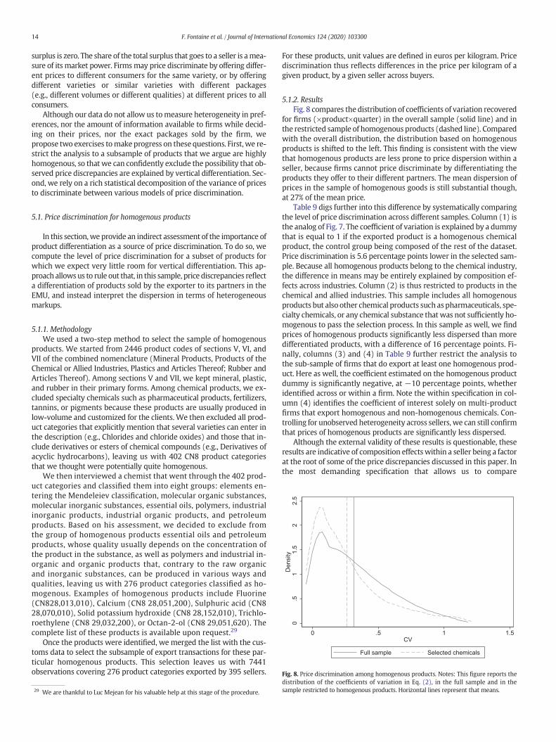
0.5

11.

52

2.5

Den

sity

0 .5 1 1.5CV

Full sample Selected chemicals

Fig. 8. Price discrimination among homogenous products. Notes: This figure reports the

14 F. Fontaine et al. / Journal of International Economics 124 (2020) 103300

surplus is zero. The share of the total surplus that goes to a seller is amea-sure of its market power. Firmsmay price discriminate by offering differ-ent prices to different consumers for the same variety, or by offeringdifferent varieties or similar varieties with different packages(e.g., different volumes or different qualities) at different prices to allconsumers.

Although our data do not allow us tomeasure heterogeneity in pref-erences, nor the amount of information available to firms while decid-ing on their prices, nor the exact packages sold by the firm, wepropose two exercises tomake progress on these questions. First, we re-strict the analysis to a subsample of products that we argue are highlyhomogenous, so that we can confidently exclude the possibility that ob-served price discrepancies are explained by vertical differentiation. Sec-ond, we rely on a rich statistical decomposition of the variance of pricesto discriminate between various models of price discrimination.

5.1. Price discrimination for homogenous products

In this section,we provide an indirect assessment of the importance ofproduct differentiation as a source of price discrimination. To do so, wecompute the level of price discrimination for a subset of products forwhich we expect very little room for vertical differentiation. This ap-proach allowsus to rule out that, in this sample, price discrepancies reflecta differentiation of products sold by the exporter to its partners in theEMU, and instead interpret the dispersion in terms of heterogeneousmarkups.

5.1.1. MethodologyWe used a two-step method to select the sample of homogenous

products. We started from 2446 product codes of sections V, VI, andVII of the combined nomenclature (Mineral Products, Products of theChemical or Allied Industries, Plastics and Articles Thereof; Rubber andArticles Thereof). Among sections V and VII, we kept mineral, plastic,and rubber in their primary forms. Among chemical products, we ex-cluded specialty chemicals such as pharmaceutical products, fertilizers,tannins, or pigments because these products are usually produced inlow-volume and customized for the clients. We then excluded all prod-uct categories that explicitly mention that several varieties can enter inthe description (e.g., Chlorides and chloride oxides) and those that in-clude derivatives or esters of chemical compounds (e.g., Derivatives ofacyclic hydrocarbons), leaving us with 402 CN8 product categoriesthat we thought were potentially quite homogenous.

We then interviewed a chemist that went through the 402 prod-uct categories and classified them into eight groups: elements en-tering the Mendeleiev classification, molecular organic substances,molecular inorganic substances, essential oils, polymers, industrialinorganic products, industrial organic products, and petroleumproducts. Based on his assessment, we decided to exclude fromthe group of homogenous products essential oils and petroleumproducts, whose quality usually depends on the concentration ofthe product in the substance, as well as polymers and industrial in-organic and organic products that, contrary to the raw organicand inorganic substances, can be produced in various ways andqualities, leaving us with 276 product categories classified as ho-mogenous. Examples of homogenous products include Fluorine(CN828,013,010), Calcium (CN8 28,051,200), Sulphuric acid (CN828,070,010), Solid potassium hydroxide (CN8 28,152,010), Trichlo-roethylene (CN8 29,032,200), or Octan-2-ol (CN8 29,051,620). Thecomplete list of these products is available upon request.29

Once the products were identified, we merged the list with the cus-toms data to select the subsample of export transactions for these par-ticular homogenous products. This selection leaves us with 7441observations covering 276 product categories exported by 395 sellers.

29 We are thankful to Luc Mejean for his valuable help at this stage of the procedure.

For these products, unit values are defined in euros per kilogram. Pricediscrimination thus reflects differences in the price per kilogram of agiven product, by a given seller across buyers.

5.1.2. ResultsFig. 8 compares the distribution of coefficients of variation recovered

for firms (×product×quarter) in the overall sample (solid line) and inthe restricted sample of homogenous products (dashed line). Comparedwith the overall distribution, the distribution based on homogenousproducts is shifted to the left. This finding is consistent with the viewthat homogenous products are less prone to price dispersion within aseller, because firms cannot price discriminate by differentiating theproducts they offer to their different partners. The mean dispersion ofprices in the sample of homogenous goods is still substantial though,at 27% of the mean price.

Table 9 digs further into this difference by systematically comparingthe level of price discrimination across different samples. Column (1) isthe analog of Fig. 7. The coefficient of variation is explained by a dummythat is equal to 1 if the exported product is a homogenous chemicalproduct, the control group being composed of the rest of the dataset.Price discrimination is 5.6 percentage points lower in the selected sam-ple. Because all homogenous products belong to the chemical industry,the difference in means may be entirely explained by composition ef-fects across industries. Column (2) is thus restricted to products in thechemical and allied industries. This sample includes all homogenousproducts but also other chemical products such as pharmaceuticals, spe-cialty chemicals, or any chemical substance that was not sufficiently ho-mogenous to pass the selection process. In this sample as well, we findprices of homogenous products significantly less dispersed than moredifferentiated products, with a difference of 16 percentage points. Fi-nally, columns (3) and (4) in Table 9 further restrict the analysis tothe sub-sample of firms that do export at least one homogenous prod-uct. Here as well, the coefficient estimated on the homogenous productdummy is significantly negative, at −10 percentage points, whetheridentified across or within a firm. Note the within specification in col-umn (4) identifies the coefficient of interest solely on multi-productfirms that export homogenous and non-homogenous chemicals. Con-trolling for unobserved heterogeneity across sellers, we can still confirmthat prices of homogenous products are significantly less dispersed.

Although the external validity of these results is questionable, theseresults are indicative of composition effectswithin a seller being a factorat the root of some of the price discrepancies discussed in this paper. Inthe most demanding specification that allows us to compare

distribution of the coefficients of variation in Eq. (2), in the full sample and in thesample restricted to homogenous products. Horizontal lines represent that means.

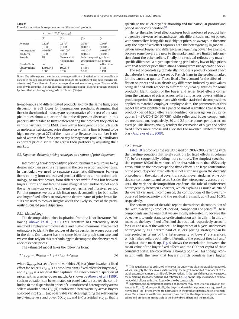
Table 9Price discrimination: homogenous versus differentiated products.

Dep. Var.: CVsptcb(c)(psb(c)pt)

(1) (2) (3) (4)

Average 0.323a 0.372a 0.369a 0.368a

(0.000) (0.001) (0.001) (0.001)Homogenous −0.056a −0.105a −0.101a −0.097a

products (0.003) (0.001) (0.004) (0.004)Sample All Chemicals & Sellers exporting at least

Allied indus. One homogenous productFixed effects no no no seller×timeObservations 1,402,748 109,676 61,851 61,851R2 0.000 0.037 0.010 0.191

Notes: The table reports the estimated average coefficient of variation, in the overall sam-ple and in the sub-sample of homogenous products (the coefficient being expressed in rel-ative terms). The different columns correspond to various control groups: The rest of theeconomy in column (1), other chemical products in column (2), other products exportedby firms that sell homogenous goods in columns (3)–(4).

30 This equation can be estimatedwhenever the underlying bipartite graph is connected,which is largely the case in our data. Namely, the largest connected component of thegraph encompassesmore than99%of all observations. In the rest of the section,we neglectthe remaining 1% of observations and estimate Eq. (6) on the largest connected compo-nent, which allows estimated fixed effects to be comparable.31 In practice, the decomposition is based on the three-way fixed-effects estimation pre-sented in Eq. (6). More specifically, the buyer and match components are regressed onnormalized (log) prices. Prices are normalized in the product×period and seller dimen-sions. The estimated coefficients measure how much of the dispersion in prices withinsellers and products is attributable to the buyer fixed effects and the residuals.

15F. Fontaine et al. / Journal of International Economics 124 (2020) 103300

homogenous and differentiated products sold by the same firm, pricedispersion is 26% lower for homogenous products. Assuming thatfirms in the chemical industry are representative of the rest of the sam-ple implies about a quarter of the price dispersion discussed in thispaper is attributable to firms differentiating the products they offer tovarious partners in the EMU. Even within homogenous products suchas molecular substances, price dispersion within a firm is found to behigh, on average, at 27% of the mean price. Because this number is ob-tained within a firm, for a particularly homogenous product, it indicatesexporters price discriminate across their partners by adjusting theirmarkup.

5.2. Exporters' dynamic pricing strategies as a source of price dispersion

Interpretingfirms' propensity to price discriminate requires us to digdeeper into their pricing strategies, in the cross-section and over time.In particular, we need to separate systematic differences betweenfirms, coming from unobserved product differences, production tech-nology, or market power, from differences within firms but betweenbuyers if firms do not face the same marginal cost and/or do not applythe samemark-ups over the different partners served in a given period.For that purpose, we use a rich linear model, controlling for both sellerand buyer fixed effects to analyze the determinants of price levels. Re-sults are used to recover insights about the likely sources of the previ-ously discussed price dispersion.

5.2.1. MethodologyThe decomposition takes inspiration from the labor literature. Fol-

lowing Abowd et al. (1999), this literature has extensively usedmatched employer-employee data and high-dimensional fixed-effectestimators to identify the sources of the dispersion in wages observedin the data. Our dataset has the same bipartite graph structure, andwe can thus rely on this methodology to decompose the observed vari-ance of export prices.

The estimated model takes the following form:

lnpsb cð Þpt ¼ βXsb cð Þpt þ FEs þ FEb cð Þ þ esb cð Þpt ð6Þ

where Xsb(c)pt is a set of control variables, FEs is a (time-invariant) fixedeffect for seller s, FEb(c) is a (time-invariant) fixed effect for buyer b(c),and esb(c)pt is a residual that captures the unexplained dispersion ofprices within a seller-buyer match. As shown by Abowd et al. (1999),such an equation can be estimated on panel data to recover the contri-bution to the dispersion in prices of (i) unobserved heterogeneity acrosssellers absorbed into FEs, (ii) unobserved heterogeneity across buyersabsorbed into FEb(c), (iii) observable variables regarding the relationshipinvolving seller s and buyer b Xsb(c)pt, and (iv) a residual esb(c)pt that is

specific to the seller-buyer relationship and the particular product andperiod under consideration.30

Hence, the seller fixed effect captures both unobserved product het-erogeneity between sellers and systematic differences inmarket power,with some sellers being able to set higher prices, on average. In the sameway, the buyer fixed effect captures both the heterogeneity in good val-uation among buyers, and differences in bargaining power, for example,because some buyers are new to the market and have limited informa-tion about the other sellers. Finally, the residual reflects any match-specific difference: a buyer experiencing particularly low or high priceswith that seller or price fluctuations coming from idiosyncratic shocks.

The set of controls systematically includes a product×period effectthat absorbs the mean price set by French firms in the product marketfor this particular quarter. These fixed effects control for the effect of in-flation on prices and also absorb any difference induced by unit valuesbeing defined with respect to different physical quantities for someproducts. Identification of the buyer and seller fixed effects comesfrom the variance of prices across sellers and across buyers within aproduct×period. In comparison with similar statistical decompositionsapplied to matched employer-employee data, the parameters of thismodel are well identified. In a panel of almost 40 millions transactions,product×period fixed effects are identified, on average, on 226 pricequotes (=37,470,412/165,730) while seller and buyer componentsare measured on, respectively, 30 and 2.3 price quotes per quarter, onaverage. This dimensionality renders the estimation of buyer and sellerfixed effects more precise and alleviates the so-called limited mobilitybias (Andrews et al., 2008).

5.2.2. ResultsTable 10 reproduces the results based on 2002–2006, starting with

the baseline equation that solely controls for fixed effects in column(1), before sequentially adding more controls. The simplest specifica-tion captures 89% of the variance of the data, with more than 65% solelyattributable to the product×period fixed effects. The large contributionof the product×period fixed effects is not surprising given the diversityof products in the data that cover transactions over airplanes, wine bot-tles, car components, and so on. Besides the heterogeneity across prod-ucts, the variance decomposition confirms the role of unobservedheterogeneity between exporters, which explains as much as 20% ofthe overall variance. In comparison, the contributions of the buyer un-observed heterogeneity and the residual are small, at 4.5 and 10.5%,respectively.

The bottom panel of the table reports the variance decomposition ofthe within-seller (×product×period) components of prices.31 Thesecomponents are the ones that we are mostly interested in, because theobjective is to understand price discrimination within a firm. In this di-mension, the buyer fixed effect and the residual, respectively, accountfor 17% and 83% of the variance. The importance of buyers' unobservedheterogeneity as a determinant of sellers' pricing strategies can beinterpreted in terms of the heterogeneity of buyers' preferences,which makes sellers optimally differentiate the product they sell and/or adjust their mark-up. Fig. 9 shows the correlation between themean value of the buyer fixed effects and the GDP per capita of theircountry of origin. The correlation is strongly positive. Thisfinding is con-sistent with the view that buyers in rich countries have higher

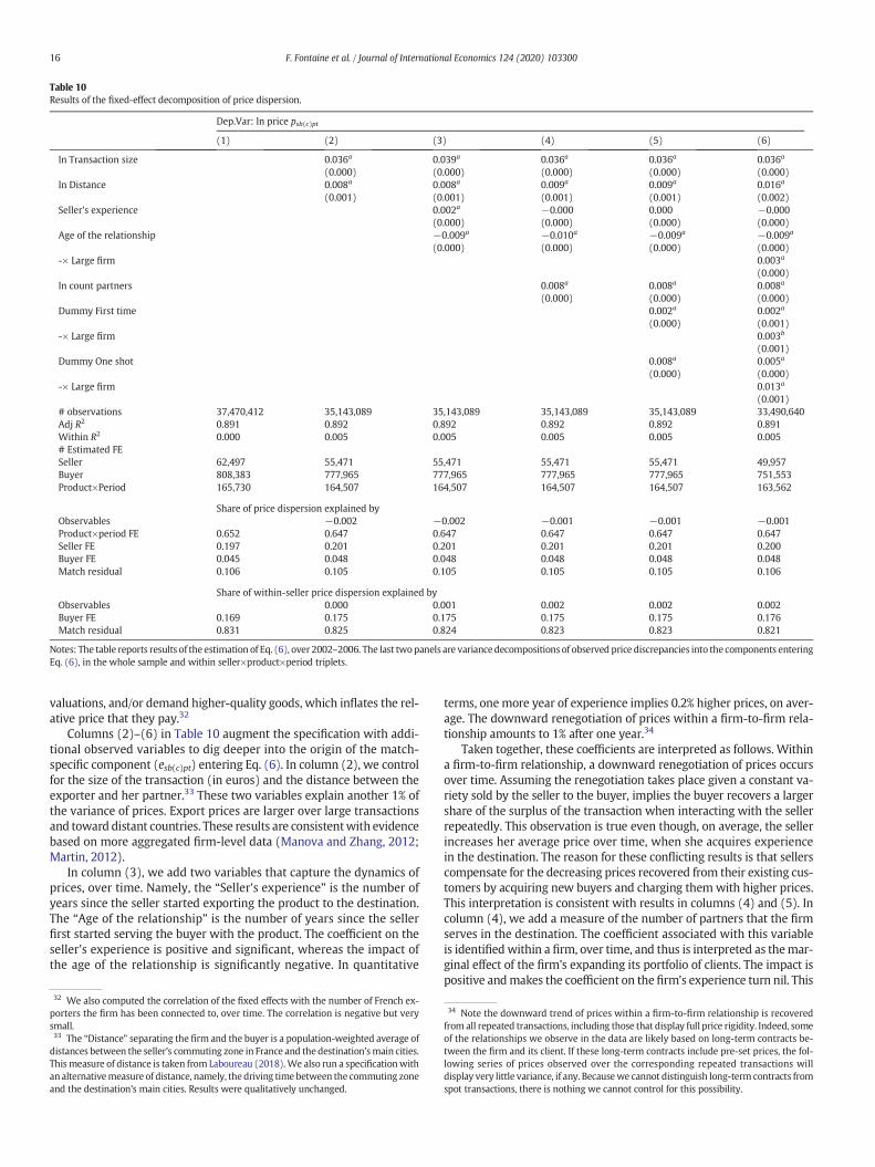
Table 10Results of the fixed-effect decomposition of price dispersion.

Dep.Var: ln price psb(c)pt

(1) (2) (3) (4) (5) (6)

ln Transaction size 0.036a 0.039a 0.036a 0.036a 0.036a

(0.000) (0.000) (0.000) (0.000) (0.000)ln Distance 0.008a 0.008a 0.009a 0.009a 0.016a

(0.001) (0.001) (0.001) (0.001) (0.002)Seller's experience 0.002a −0.000 0.000 −0.000

(0.000) (0.000) (0.000) (0.000)Age of the relationship −0.009a −0.010a −0.009a −0.009a

(0.000) (0.000) (0.000) (0.000)-× Large firm 0.003a

(0.000)ln count partners 0.008a 0.008a 0.008a

(0.000) (0.000) (0.000)Dummy First time 0.002a 0.002a

(0.000) (0.001)-× Large firm 0.003b

(0.001)Dummy One shot 0.008a 0.005a

(0.000) (0.000)-× Large firm 0.013a

(0.001)# observations 37,470,412 35,143,089 35,143,089 35,143,089 35,143,089 33,490,640Adj R2 0.891 0.892 0.892 0.892 0.892 0.891Within R2 0.000 0.005 0.005 0.005 0.005 0.005# Estimated FESeller 62,497 55,471 55,471 55,471 55,471 49,957Buyer 808,383 777,965 777,965 777,965 777,965 751,553Product×Period 165,730 164,507 164,507 164,507 164,507 163,562

Share of price dispersion explained byObservables −0.002 −0.002 −0.001 −0.001 −0.001Product×period FE 0.652 0.647 0.647 0.647 0.647 0.647Seller FE 0.197 0.201 0.201 0.201 0.201 0.200Buyer FE 0.045 0.048 0.048 0.048 0.048 0.048Match residual 0.106 0.105 0.105 0.105 0.105 0.106

Share of within-seller price dispersion explained byObservables 0.000 0.001 0.002 0.002 0.002Buyer FE 0.169 0.175 0.175 0.175 0.175 0.176Match residual 0.831 0.825 0.824 0.823 0.823 0.821

Notes: The table reports results of the estimation of Eq. (6), over 2002–2006. The last twopanels are variancedecompositions of observed price discrepancies into the components enteringEq. (6), in the whole sample and within seller×product×period triplets.

16 F. Fontaine et al. / Journal of International Economics 124 (2020) 103300

valuations, and/or demand higher-quality goods, which inflates the rel-ative price that they pay.32

Columns (2)–(6) in Table 10 augment the specification with addi-tional observed variables to dig deeper into the origin of the match-specific component (esb(c)pt) entering Eq. (6). In column (2), we controlfor the size of the transaction (in euros) and the distance between theexporter and her partner.33 These two variables explain another 1% ofthe variance of prices. Export prices are larger over large transactionsand toward distant countries. These results are consistentwith evidencebased on more aggregated firm-level data (Manova and Zhang, 2012;Martin, 2012).

In column (3), we add two variables that capture the dynamics ofprices, over time. Namely, the “Seller's experience” is the number ofyears since the seller started exporting the product to the destination.The “Age of the relationship” is the number of years since the sellerfirst started serving the buyer with the product. The coefficient on theseller's experience is positive and significant, whereas the impact ofthe age of the relationship is significantly negative. In quantitative

32 We also computed the correlation of the fixed effects with the number of French ex-porters the firm has been connected to, over time. The correlation is negative but verysmall.33 The “Distance” separating the firm and the buyer is a population-weighted average ofdistances between the seller's commuting zone in France and the destination'smain cities.This measure of distance is taken from Laboureau (2018).We also run a specificationwithanalternativemeasure of distance, namely, the driving time between the commuting zoneand the destination's main cities. Results were qualitatively unchanged.

terms, onemore year of experience implies 0.2% higher prices, on aver-age. The downward renegotiation of prices within a firm-to-firm rela-tionship amounts to 1% after one year.34

Taken together, these coefficients are interpreted as follows. Withina firm-to-firm relationship, a downward renegotiation of prices occursover time. Assuming the renegotiation takes place given a constant va-riety sold by the seller to the buyer, implies the buyer recovers a largershare of the surplus of the transaction when interacting with the sellerrepeatedly. This observation is true even though, on average, the sellerincreases her average price over time, when she acquires experiencein the destination. The reason for these conflicting results is that sellerscompensate for the decreasing prices recovered from their existing cus-tomers by acquiring new buyers and charging them with higher prices.This interpretation is consistent with results in columns (4) and (5). Incolumn (4), we add a measure of the number of partners that the firmserves in the destination. The coefficient associated with this variableis identifiedwithin a firm, over time, and thus is interpreted as themar-ginal effect of the firm's expanding its portfolio of clients. The impact ispositive andmakes the coefficient on the firm's experience turn nil. This

34 Note the downward trend of prices within a firm-to-firm relationship is recoveredfrom all repeated transactions, including those that display full price rigidity. Indeed, someof the relationships we observe in the data are likely based on long-term contracts be-tween the firm and its client. If these long-term contracts include pre-set prices, the fol-lowing series of prices observed over the corresponding repeated transactions willdisplay very little variance, if any. Becausewe cannot distinguish long-term contracts fromspot transactions, there is nothing we cannot control for this possibility.

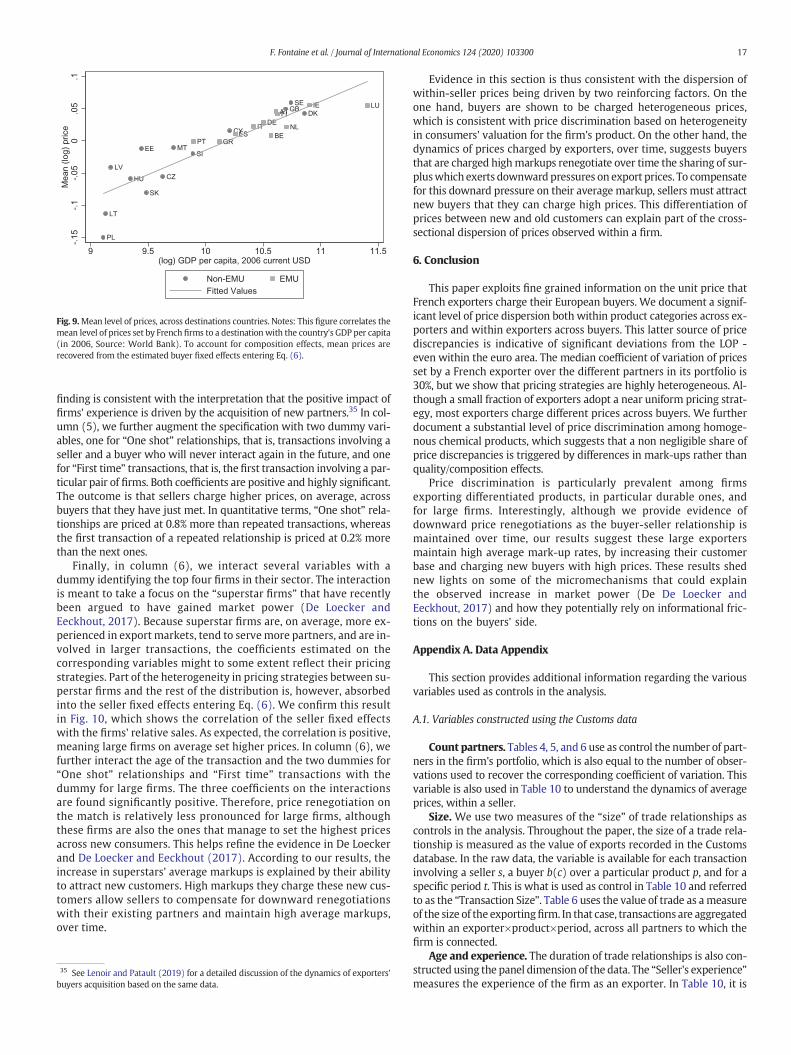
AT

BECY

CZ

DEDK

EE

ES

FIGB

GR

HU

IE

IT

LT

LU

LV

MT

NL

PL

PT

SE

SI

SK

-.15

-.1

-.05

0.0

5.1

Mea

n (lo

g) p

rice

9 9.5 10 10.5 11 11.5(log) GDP per capita, 2006 current USD

Non-EMU EMUFitted Values

Fig. 9.Mean level of prices, across destinations countries. Notes: This figure correlates themean level of prices set by French firms to a destination with the country's GDP per capita(in 2006, Source: World Bank). To account for composition effects, mean prices arerecovered from the estimated buyer fixed effects entering Eq. (6).

17F. Fontaine et al. / Journal of International Economics 124 (2020) 103300

finding is consistent with the interpretation that the positive impact offirms' experience is driven by the acquisition of new partners.35 In col-umn (5), we further augment the specification with two dummy vari-ables, one for “One shot” relationships, that is, transactions involving aseller and a buyer who will never interact again in the future, and onefor “First time” transactions, that is, the first transaction involving a par-ticular pair of firms. Both coefficients are positive and highly significant.The outcome is that sellers charge higher prices, on average, acrossbuyers that they have just met. In quantitative terms, “One shot” rela-tionships are priced at 0.8% more than repeated transactions, whereasthe first transaction of a repeated relationship is priced at 0.2% morethan the next ones.

Finally, in column (6), we interact several variables with adummy identifying the top four firms in their sector. The interactionis meant to take a focus on the “superstar firms” that have recentlybeen argued to have gained market power (De Loecker andEeckhout, 2017). Because superstar firms are, on average, more ex-perienced in export markets, tend to servemore partners, and are in-volved in larger transactions, the coefficients estimated on thecorresponding variables might to some extent reflect their pricingstrategies. Part of the heterogeneity in pricing strategies between su-perstar firms and the rest of the distribution is, however, absorbedinto the seller fixed effects entering Eq. (6). We confirm this resultin Fig. 10, which shows the correlation of the seller fixed effectswith the firms' relative sales. As expected, the correlation is positive,meaning large firms on average set higher prices. In column (6), wefurther interact the age of the transaction and the two dummies for“One shot” relationships and “First time” transactions with thedummy for large firms. The three coefficients on the interactionsare found significantly positive. Therefore, price renegotiation onthe match is relatively less pronounced for large firms, althoughthese firms are also the ones that manage to set the highest pricesacross new consumers. This helps refine the evidence in De Loeckerand De Loecker and Eeckhout (2017). According to our results, theincrease in superstars' average markups is explained by their abilityto attract new customers. High markups they charge these new cus-tomers allow sellers to compensate for downward renegotiationswith their existing partners and maintain high average markups,over time.

35 See Lenoir and Patault (2019) for a detailed discussion of the dynamics of exporters'buyers acquisition based on the same data.

Evidence in this section is thus consistent with the dispersion ofwithin-seller prices being driven by two reinforcing factors. On theone hand, buyers are shown to be charged heterogeneous prices,which is consistent with price discrimination based on heterogeneityin consumers' valuation for the firm's product. On the other hand, thedynamics of prices charged by exporters, over time, suggests buyersthat are charged highmarkups renegotiate over time the sharing of sur-pluswhich exerts downward pressures on export prices. To compensatefor this downard pressure on their average markup, sellers must attractnew buyers that they can charge high prices. This differentiation ofprices between new and old customers can explain part of the cross-sectional dispersion of prices observed within a firm.

6. Conclusion

This paper exploits fine grained information on the unit price thatFrench exporters charge their European buyers. We document a signif-icant level of price dispersion both within product categories across ex-porters and within exporters across buyers. This latter source of pricediscrepancies is indicative of significant deviations from the LOP -even within the euro area. The median coefficient of variation of pricesset by a French exporter over the different partners in its portfolio is30%, but we show that pricing strategies are highly heterogeneous. Al-though a small fraction of exporters adopt a near uniform pricing strat-egy, most exporters charge different prices across buyers. We furtherdocument a substantial level of price discrimination among homoge-nous chemical products, which suggests that a non negligible share ofprice discrepancies is triggered by differences in mark-ups rather thanquality/composition effects.

Price discrimination is particularly prevalent among firmsexporting differentiated products, in particular durable ones, andfor large firms. Interestingly, although we provide evidence ofdownward price renegotiations as the buyer-seller relationship ismaintained over time, our results suggest these large exportersmaintain high average mark-up rates, by increasing their customerbase and charging new buyers with high prices. These results shednew lights on some of the micromechanisms that could explainthe observed increase in market power (De De Loecker andEeckhout, 2017) and how they potentially rely on informational fric-tions on the buyers' side.

Appendix A. Data Appendix

This section provides additional information regarding the variousvariables used as controls in the analysis.

A.1. Variables constructed using the Customs data

Count partners. Tables 4, 5, and 6 use as control the number of part-ners in the firm's portfolio, which is also equal to the number of obser-vations used to recover the corresponding coefficient of variation. Thisvariable is also used in Table 10 to understand the dynamics of averageprices, within a seller.

Size. We use two measures of the “size” of trade relationships ascontrols in the analysis. Throughout the paper, the size of a trade rela-tionship is measured as the value of exports recorded in the Customsdatabase. In the raw data, the variable is available for each transactioninvolving a seller s, a buyer b(c) over a particular product p, and for aspecific period t. This is what is used as control in Table 10 and referredto as the “Transaction Size”. Table 6 uses the value of trade as ameasureof the size of the exportingfirm. In that case, transactions are aggregatedwithin an exporter×product×period, across all partners to which thefirm is connected.

Age and experience. The duration of trade relationships is also con-structed using the panel dimension of the data. The “Seller's experience”measures the experience of the firm as an exporter. In Table 10, it is

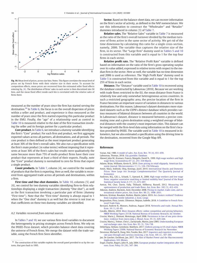
-.3

-.2

-.1

0.1

Mea

n se

ller

fixed

effe

ct

-2 0 2 4 6 8log Relative sales

Fig. 10.Mean level of prices, across size bins.Notes: Thisfigure correlates themean level ofprices set by French firms with their relative size in their sector. To account forcomposition effects, mean prices are recovered from the estimated seller fixed effectsentering Eq. (6). The distribution of firms' sales in each sector is then discretized into 50bins, and the mean fixed effect inside each bin is correlated with the relative sales offirms there.

18 F. Fontaine et al. / Journal of International Economics 124 (2020) 103300

measured as the number of years since the firm has started serving thedestination.36 In Table 6, the focus is on the overall dispersion of priceswithin a seller and product, and experience is thus measured as thenumber of years since the firm started exporting this particular productin the EMU. Finally, the “age” of a relationship used as control inTable 10 is measured relative to the date of the first transaction involv-ing the seller and its foreign partner for a particular product.

Core product. In Table 6,we introduce a dummyvariable identifyingthe firm's “Core” product. For each firm and product, we first aggregateexported values across all partners, all destinations, and all periods. Thecore product is then defined as the most important product generatingat least 30% of the firm's overall sales. We also run a specification withthefirm'smain product (in value terms)without imposing that it repre-sents at least 30% of the firm's sales but results were qualitatively thesame because more than 75% of multi-product firms have their coreproduct that represents at least a third of their exports. Finally, notethe “Core” product dummy is normalized to zero for firms that exporta single product.

Count products. In Table 7, column (4), we control for the numberof products that thefirm is exporting. Here aswell, the variable is recov-ered from aggregated trade across all periods and destinations, withina firm.

First time and One-shot dummies. In Table 10, columns (5) and(6), we control for two dummy variables identifying firm-to-firm rela-tionships displaying a single transaction (dummy “One shot”), as wellas the first transaction involving a particular pair of firms (dummy“First time”). Note that the “First time” dummy is always equal to 1when the “One shot” dummy is as well but the reverse is not true sothat coefficients on these two dummy variables are identified.

A.2. Variables recovered from external sources

In Tables 7 and 10, we use various firm-level variables to documentthe heterogeneity in pricing strategies across French firms. We rely onthe INSEE-Ficus dataset, which provides balance-sheet data coveringthe universe of French firms. We merge the dataset with the trade var-iable, using the French firm Siren identifier.

36 The construction of this variable exploits the overall panel provided to us by the cus-toms, that goes back to 1995.

Sector. Based on the balance-sheet data,we can recover informationon the firm's sector of activity, as defined in the NAF nomenclature. Weuse this information to construct the “Wholesaler” and “Retailer”dummies introduced in column (3) of Table 7.

Relative sales. The “Relative Sales” variable in Table 7 is measuredas the ratio of the firm's overall turnover divided by themedian turn-over of firms active in the same sector of activity. We get rid of thetime dimension by calculating this ratio for a single cross-section,namely, 2006. The variable thus captures the relative size of thefirm, in its sector. The “Large firm” dummy used in Tables 5 and 10is constructed from this variable and is equal to 1 for the top fourfirms in each sector.

Relative profit rate. The “Relative Profit Rate” variable is definedbased on information on the ratio of the firm's gross operating surplusover its value added, expressed in relative termswith respect to theme-dian firm in the sector. Here aswell, the variable has no time dimensionand 2006 is used as reference. The ‘High Profit Rate” dummy used inTable 5 is constructed from this variable and is equal to 1 for the top25% of firms in each sector.

Distance. The “Distance” variable used in Table 10 is recovered usingthe database constructed by Laboureau (2018). Becausewe areworkingwith trade flows restricted to the EU, the mean distance from France isrelatively low and only somewhat heterogeneous across countries. Insuch a restricted geographic area, the precise location of the firm inFrance becomes an important source of variation in distances to variousdestinations. For this reason, Laboureau's dataset dominates more stan-dard datasets such as the CEPII's distance database which provides var-ious measures of bilateral distances between all countries in the world.In Laboureau's dataset, distance is measured between a precise com-muting zone and a given destination using a weighted average of bilat-eral distances with the country's most important cities. This dataset canbemergedwith thefirm-level data using information on thefirm's loca-tion provided by INSEE. The variable used in Table 10 is measured in ki-lometers, but we also estimated a specification using the driving time tothe destination, recovered from the Google Map API.

References

Varian, Hal, 1980. A model of sales. Am. Econ. Rev. 70 (4), 651–659.Laboureau, Thomas, 2018. City gravidist. Database.Abowd, John M., Kramarz, Francis, Margolis, David N., 1999. High wage workers and high

wage firms. Econometrica 67 (2), 251–334 March.Adams, Brian, Williams, Kevin R., 2019. Zone pricing in retail oligopoly. American Eco-

nomic Journal: Microeconomics 11 (1), 124–156 February.Amiti, Mary, Itskhoki, Oleg, Konings, Jozef, 2019. International Shocks and Domestic

Prices: How Large Are Strategic Complementarities? The Quarterly Journal ofEconomics

Andrews, M.J., Gill, L., Schank, T., Upward, R., 2008. High wage workers and low wagefirms: negative assortative matching or limited mobility bias? Journal of the RoyalStatistical Society Series A 171 (3), 673–697.

Antras, Pol, Chor, Davin, Fally, Thibault, Hillberry, Russell, 2012. Measuring theupstreamness of production and trade flows. Am. Econ. Rev. 102 (3), 412–416.

Atkeson, Andrew, Burstein, Ariel, December 2008. Pricing-to-market, trade costs, and in-ternational relative prices. Am. Econ. Rev. 98 (5), 1998–2031.

Behrens, Kristian, Boualam, Brahim, Martin, Julien, 2019. Are clusters resilient? Evidencefrom Canadian textile industries. J. Econ. Geogr.

Bergounhon, Flora, Lenoir, Clémence, Mejean, Isabelle, 2018. A Guideline to French Firm-Level Trade Data.

Bernard, Andrew B., Moxnes, Andreas, August 2018. Networks and trade. Annual Rev.Econ. 10 (1), 65–85.

Cavallo, Alberto, 2018. More Amazon effects: online competition and pricing behaviors.NBER Working Papers 25138. National Bureau of Economic Research, Inc October.

Crucini, Mario J., Shintani, Mototsugu, April 2008. Persistence in law of one price devia-tions: evidence from micro-data. J. Monet. Econ. 55 (3), 629–644.

Crucini, Mario J., Telmer, Chris I., Zachariadis, Marios, June 2005. Understanding Europeanreal exchange rates. Am. Econ. Rev. 95 (3), 724–738.

DellaVigna, Stefano, Gentzkow, Matthew, 2017. Uniform pricing in US retail chains. NBERWorking Papers 23996. National Bureau of Economic Research Inc November.

Devereux, Michael B., Dong, Wei, Tomlin, Ben, 2017. Importers and exporters in exchangerate pass-through and currency invoicing. J. Int. Econ. 105 (C), 187–204.

Jan, De Loecker, Eeckhout, Jan, 2017. The Rise of Market Power and the MacroeconomicImplications. UCL Mimeo.

Engel, Charles, Rogers, John H., July 2004. European product market integration after theeuro. Econ. Policy 19 (39), 347–384.

19F. Fontaine et al. / Journal of International Economics 124 (2020) 103300

Engel, Charles, Wang, Jian, January 2011. International trade in durable goods: under-standing volatility, cyclicality, and elasticities. J. Int. Econ. 83 (1), 37–52.

Fitzgerald, Doireann, Haller, Stefanie, 2014. Pricing-to-market: evidence from plant-levelprices. Review of Economic Studies 81 (2), 761–786.

Goldberg, Linda S., Tille, Cédric, 2016. Micro, macro, and strategic forces in internationaltrade invoicing: synthesis and novel patterns. J. Int. Econ. 102 (C), 173–187.

Goldberg, Pinelopi K., Verboven, Frank, January 2005. Market integration and conver-gence to the law of one price: evidence from the European car market. J. Int. Econ.65 (1), 49–73.

Gopinath, Gita, Gourinchas, Pierre-Olivier, Hsieh, Chang-Tai, Li, Nicholas, October 2011.International prices, costs, and markup differences. Am. Econ. Rev. 101 (6),2450–2486.

Hausmann, Ricardo, Hidalgo, Cesar, 2014. The Atlas of Economic Complexity: MappingPaths to Prosperity. Vol. 1. MIT Press Books, The MIT Press January.

Engel, Charles, John, H., 1996. Rogers, how wide is the border? Am. Econ. Rev. 86 (5),1112–1125 December.

Kaplan, Greg, Menzio, Guido, November 2015. The morphology of price dispersion. Int.Econ. Rev. 56, 1165–1206.

Lenoir, Clemence, Patault, Berangere, 2019. Exporters Dynamics: Sales Managers andFirm's International Portfolios.

Levchenko, Andrei A., Lewis, Logan T., Tesar, Linda L., 2010. The collapse of internationaltrade during the 2008âĂŞ09 crisis: in search of the smoking gun. IMF Economic Re-view 58 (2), 214–253 December.

Manova, Kalina, Zhang, Zhiwei, 2012. Export prices across firms and destinations. Q.J. Econ. 127 (1), 379–436.

Martin, Julien, 2012. Markups, quality, and transport costs. Eur. Econ. Rev. 56 (4),777–791.

Berman, Nicolas, Martin, Philippe, Mayer, Thierry, 2012. How do different exporters reactto exchange rate changes? Q. J. Econ. 127 (1), 437–492.

Martin, Julien, Mejean, Isabelle, Parenti, Mathieu, 2019. Relationship Stickiness: Measure-ment and Applications to International Economics.

Cavallo, Alberto, Neiman, Brent, Rigobon, Roberto, 2014. Currency unions, product intro-ductions and the real exchange rate. The Quarterly Journal of Economics 129 (2),529–595.

Nunn, Nathan, 2007. Relationship-specificity, incomplete contracts, and the pattern oftrade. Q. J. Econ. 122 (2), 569–600.

Rauch, James E., June 1999. Networks versusmarkets in international trade. J. Int. Econ. 48(1), 7–35.

Stigler, George J., Jun., 1961. The economics of information. J. Polit. Econ. 69 (3), 213–225.Tirole, Jean, 1988. The Theory of Industrial Organization. Vol. 1. MIT Press Books, The MIT

Press March.