Journal of Forest Economics - Southern Research · J. Buongiorno et al. / Journal of Forest Economics 17 (2011) 214–229 219 by 2030. The price of sawnwood would approximately follow

Journal of Forest Economics 17 (2011) 214–229

Contents lists available at ScienceDirect

Journal of Forest Economics

journa l homepage: www.e lsev ier .de / j fe

Consequences of increasing bioenergy demand on woodand forests: An application of the Global Forest ProductsModel

Joseph Buongiornoa,∗, Ronald Raunikarb, Shushuai Zhua

a Department of Forest and Wildlife Ecology, University of Wisconsin, Madison, WI, USAb US Geological Survey, Menlo Park, CA, USA

a r t i c l e i n f o

Article history:Received 19 July 2010Accepted 11 February 2011

JEL classification:C54C61F18L73O13A23Q41

Keywords:Forest sectorModelingBioenergyFuelwoodWood productsPricesDemandSupplyTrade

a b s t r a c t

The Global Forest Products Model (GFPM) was applied to projectthe consequences for the global forest sector of doubling the rateof growth of bioenergy demand relative to a base scenario, otherdrivers being maintained constant. The results showed that thiswould lead to the convergence of the price of fuelwood and indus-trial roundwood, raising the price of industrial roundwood bynearly 30% in 2030. The price of sawnwood and panels would be15% higher. The price of paper would be 3% higher. Concurrently,the demand for all manufactured wood products would be lowerin all countries, but the production would rise in countries withcompetitive advantage. The global value added in wood processingindustries would be 1% lower in 2030. The forest stock would be2% lower for the world and 4% lower for Asia. These effects variedsubstantially by country.

© 2011 Department of Forest Economics, SLU Umeå, Sweden.Published by Elsevier GmbH. All rights reserved.

∗ Corresponding author. Tel.: +1 608 262 0091; fax: +1 608 262 9922.E-mail address: [email protected] (J. Buongiorno).

1104-6899/$ – see front matter © 2011 Department of Forest Economics, SLU Umeå, Sweden. Published by Elsevier GmbH. All rights reserved.doi:10.1016/j.jfe.2011.02.008

dx.doi.org/10.1016/j.jfe.2011.02.008

http://www.sciencedirect.com/science/journal/11046899

http://www.elsevier.de/jfe

mailto:[email protected]

dx.doi.org/10.1016/j.jfe.2011.02.008

J. Buongiorno et al. / Journal of Forest Economics 17 (2011) 214–229 215

Introduction

This study was part of the 2010 Forest Assessment of the USDA Forest Service, mandated by theResources Planning Act (RPA). One goal is to fit the national assessment in its global context. Thus, thetrade of the United States, and the related demand, supply and prices should be consistent with globaldevelopments.

Two of the tools used for the Forest Assessment are the Global Forest Products Model (GFPM,Buongiorno et al., 2003), and the United States Forest Products Module (USFPM, Kramp and Ince, 2010)which has the same structure as the GFPM but a finer description of products and regions within theUnited States.

The 2010 RPA Forest Assessment uses scenarios of the Intergovernmental Panel on Climate Change(IPCC) (Nakicenovic et al., 2000). The IPCC scenarios project global and regional economic activity,population, land uses, and greenhouse gases. Each scenario also projects biofuel demand, which couldhave serious implications for forests and related industries.

Biomass energy consumption may increase by as much as five to seven times by 2050 (Alcamoet al., 2005). Kirilenko and Sedjo (2007) note that past estimates of the impact of climate change (e.g.,IPPC, 2001; Perez-Garcia et al., 2002; Sohngen and Mendelsohn, 1998) have tended to ignore thispotentially large demand.

Raunikar et al. (2010) did recognize the effects of bioenergy demand on forests in comparing theIPCC scenarios A1B and A2, but since other assumptions are not the same in the two scenarios (inparticular, economic and demographic growth are quite different in A1B and A2), one cannot identifythe partial effect of bioenergy demand from that study. Other previous studies that have dealt quan-titatively with the economics of wood bioenergy supply and demand, and its implications for forestshave concerned more national or regional issues. In particular, Stennes et al. (2010) have studied theimplications of expanding bioenergy production from wood in British Columbia with a regional woodfiber allocation model, while Bright et al. (2010) made an environmental assessment of wood-basedbiofuel production and consumption scenarios in Norway, with their implications for the trade ofpaper products.

This paper attempts to determine, other things being equal, the consequences for the world forestsector and specific countries of a fast acceleration of bioenergy demand. The next part of the paperdescribes how the GFPM was used for this purpose. The results, consisting of projections to 2030 arethen presented for the production, consumption, and prices, of various products, globally and for themain countries. The paper concludes with a discussion of the method and the potential for furtherdevelopments.

Methods

The GFPM model

The Global Forest Products Model is a spatial dynamic economic model of the forest sector (seeAppendix A). The model is dynamic: the equilibrium in a particular year is a function of the equilibriumin the previous year. It assumes that markets work optimally in the short-run (one year) to maximizeconsumer and producer surplus for all products in all countries (Samuelson, 1952). It further assumesthat imperfect foresight prevails over longer time periods so that there is no inter temporal optimiza-tion but a recursive dependency of the current equilibrium on the past, along the principles originallyproposed by Day (1973), and implemented in the dynamic part of the GFPM as shown in AppendixA. Validation with historical data suggests that this is a plausible approach to model the global forestsector (Buongiorno et al., 2003, pp. 75–88).

The GFPM and several applications are described in detail in Buongiorno et al. (2003). The cur-rent version of the model, together with the software, data, and documentation are available at:http://fwe.wisc.edu/facstaff/buongiorno/.

The GFPM recognizes 180 individual countries and their interaction through imports and exports.In each country the model simulates the changes in forest area and forest stock. It also calculates theconsumption, production, trade, and prices, of 14 commodity groups covering fuelwood, industrial

http://fwe.wisc.edu/facstaff/buongiorno/

216 J. Buongiorno et al. / Journal of Forest Economics 17 (2011) 214–229

roundwood, sawnwood, wood-based panels, pulp, paper and paperboard. For each year the modelalso predicts the value added by manufacturing wood in all industries.

The estimation of the demand elasticity parameters followed Simangunsong and Buongiorno(2001), and the timber supply parameters were based on Turner et al. (2006), updated with more recentdata. Buongiorno et al. (2001), updated and supplemented by Zhu et al. (2009) explain the estimationof the input–output parameters and the corresponding manufacturing cost. The main databases werethe FAOSTAT (FAO, 2008a) for production, trade, and price statistics, the FAO global forest resourceassessment (FAO, 2006) for forest area, and forest stock, and the World Bank Development IndicatorsData Base (World Bank, 2008).

Scenarios

The consequences of increased bioenergy demand were determined by comparing two scenariosthat differed only by the future demand for bioenergy. The high scenario was the scenario A1B of theIPCC. Scenario A1B is one of the three scenarios selected for the 2010 RPA Forest Assessment (USDAForest Service, 2008). It reflects a particular “storyline” about the direction of global social, economic,technical and policy developments, and interaction between developing and industrialized countries.We used scenario A1B because it assumes a high level of future bioenergy demand, and thus couldreveal the effect of such a strong policy compared to a more moderate level of future demand.

The scenario A1B assumes continuing globalization, with high income growth and low populationgrowth. Furthermore, scenario A1B projects a very rapid growth of bioenergy demand. From 2006 to2030 the global consumption of biofuel would increase by approximately 80%.

In contrast, the alternative low scenario assumed that the global demand of biofuel would riseapproximately 20% from 2006 to 2030. Meanwhile, the same assumptions were made as for the highscenario concerning the other drivers. Thus, comparison of the low and high scenario showed thepartial effect of increased bioenergy demand, other things being equal.

For the GFPM simulations, the three same exogenous variables for both scenarios were the growthof GDP and population, change in forest area, and the growth of fuelwood demand. National GDPgrowth was deducted from the regional growth so that the regional growth was the same as in theIPCC scenario A1B and the growth of individual countries converged towards this average regionalgrowth rate.

The national growth rates of forest area projected from the environmental Kuznet’s curve (Eq. (15)in Appendix A) were adjusted so that the regional area change would match that of the IPCC regionalprojections for scenario, as shown in Appendix A.

For the high scenario, the demand for fuelwood was shifted at national rates that led to the sameglobal growth as that of world bioenergy demand in the A1B scenario, an 80% increase from 2006 to2030, while assuming that the ratio of fuelwood consumption to GDP would converge over time. Forthe low scenario, the demand for fuelwood shifted in all countries at half the annual rate of the growthin the high scenario, leading to a 20% increase in fuelwood demand from 2006 to 2030.

Given these assumptions, the quantity-price equilibrium in each country, and the correspondingtrade, were computed by the GFPM. As formulated, the model allowed transformation of part of theindustrial roundwood (i.e. wood used in the past to make sawnwood, panels, and pulp) into fuelwood,when the price of fuelwood reached the price of industrial roundwood.

Results

Projected fuelwood consumption

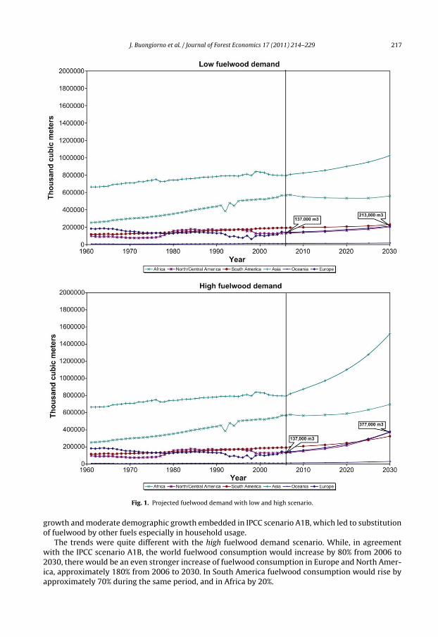
Fig. 1 shows the growth of fuelwood consumption, by main world region, from 2006 to 2030,according to the low and high fuelwood demand. In accord with FAO’s definition, fuelwood includeswood used for heating, cooking, and power production (FAO, 2008b). In the low projections, whilethe global fuelwood consumption would increase by approximately 20% from 2006 to 2030, it wouldincrease by almost 60% in Europe and North America, 30% in Asia, and 20% in South America. Theprojected slight decline of fuelwood consumption in Africa was due to the assumption of fast economic


Fig. 1. Projected fuelwood demand with low and high scenario.

growth and moderate demographic growth embedded in IPCC scenario A1B, which led to substitutionof fuelwood by other fuels especially in household usage.

The trends were quite different with the high fuelwood demand scenario. While, in agreementwith the IPCC scenario A1B, the world fuelwood consumption would increase by 80% from 2006 to2030, there would be an even stronger increase of fuelwood consumption in Europe and North Amer-ica, approximately 180% from 2006 to 2030. In South America fuelwood consumption would rise byapproximately 70% during the same period, and in Africa by 20%.


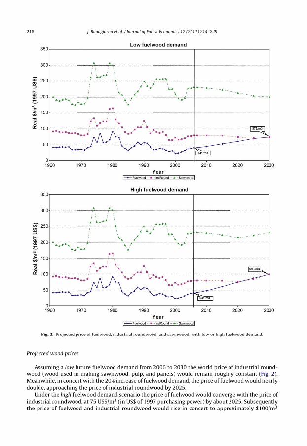
Fig. 2. Projected price of fuelwood, industrial roundwood, and sawnwood, with low or high fuelwood demand.

Projected wood prices

Assuming a low future fuelwood demand from 2006 to 2030 the world price of industrial round-wood (wood used in making sawnwood, pulp, and panels) would remain roughly constant (Fig. 2).Meanwhile, in concert with the 20% increase of fuelwood demand, the price of fuelwood would nearlydouble, approaching the price of industrial roundwood by 2025.

Under the high fuelwood demand scenario the price of fuelwood would converge with the price ofindustrial roundwood, at 75 US$/m3 (in US$ of 1997 purchasing power) by about 2025. Subsequentlythe price of fuelwood and industrial roundwood would rise in concert to approximately $100/m3


by 2030. The price of sawnwood would approximately follow the trend of the price of industrialroundwood, as it has in the past since roundwood is the main cost of sawnwood production.

The remainder of the paper focuses on the consequences of a rise in fuelwood demand, other thingsbeing equal. Thus, the following results present the effects of the change in fuelwood demand betweenthe low and the high scenario, i.e. a doubling of the rate of growth of demand, with all the other drivingvariables changing as in the A1B scenario.

Consequences for wood raw material

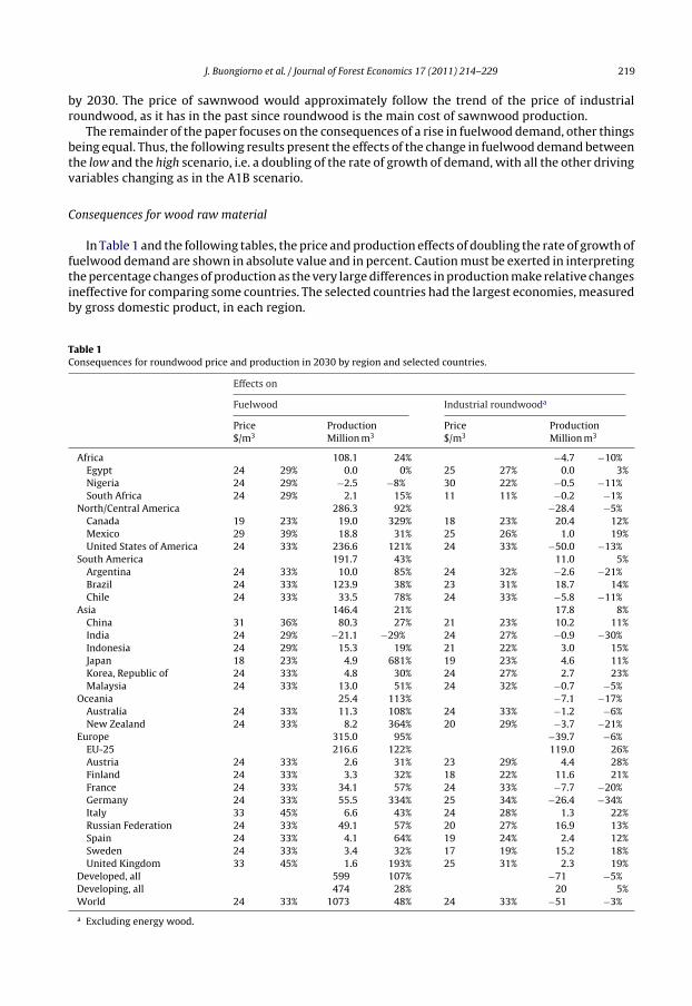
In Table 1 and the following tables, the price and production effects of doubling the rate of growth offuelwood demand are shown in absolute value and in percent. Caution must be exerted in interpretingthe percentage changes of production as the very large differences in production make relative changesineffective for comparing some countries. The selected countries had the largest economies, measuredby gross domestic product, in each region.

Table 1Consequences for roundwood price and production in 2030 by region and selected countries.

Effects on

Fuelwood Industrial roundwooda

Price$/m3

ProductionMillion m3

Price$/m3

ProductionMillion m3

Africa 108.1 24% −4.7 −10%Egypt 24 29% 0.0 0% 25 27% 0.0 3%Nigeria 24 29% −2.5 −8% 30 22% −0.5 −11%South Africa 24 29% 2.1 15% 11 11% −0.2 −1%

North/Central America 286.3 92% −28.4 −5%Canada 19 23% 19.0 329% 18 23% 20.4 12%Mexico 29 39% 18.8 31% 25 26% 1.0 19%United States of America 24 33% 236.6 121% 24 33% −50.0 −13%

South America 191.7 43% 11.0 5%Argentina 24 33% 10.0 85% 24 32% −2.6 −21%Brazil 24 33% 123.9 38% 23 31% 18.7 14%Chile 24 33% 33.5 78% 24 33% −5.8 −11%

Asia 146.4 21% 17.8 8%China 31 36% 80.3 27% 21 23% 10.2 11%India 24 29% −21.1 −29% 24 27% −0.9 −30%Indonesia 24 29% 15.3 19% 21 22% 3.0 15%Japan 18 23% 4.9 681% 19 23% 4.6 11%Korea, Republic of 24 33% 4.8 30% 24 27% 2.7 23%Malaysia 24 33% 13.0 51% 24 32% −0.7 −5%

Oceania 25.4 113% −7.1 −17%Australia 24 33% 11.3 108% 24 33% −1.2 −6%New Zealand 24 33% 8.2 364% 20 29% −3.7 −21%

Europe 315.0 95% −39.7 −6%EU-25 216.6 122% 119.0 26%Austria 24 33% 2.6 31% 23 29% 4.4 28%Finland 24 33% 3.3 32% 18 22% 11.6 21%France 24 33% 34.1 57% 24 33% −7.7 −20%Germany 24 33% 55.5 334% 25 34% −26.4 −34%Italy 33 45% 6.6 43% 24 28% 1.3 22%Russian Federation 24 33% 49.1 57% 20 27% 16.9 13%Spain 24 33% 4.1 64% 19 24% 2.4 12%Sweden 24 33% 3.4 32% 17 19% 15.2 18%United Kingdom 33 45% 1.6 193% 25 31% 2.3 19%

Developed, all 599 107% −71 −5%Developing, all 474 28% 20 5%World 24 33% 1073 48% 24 33% −51 −3%

a Excluding energy wood.


According to Table 1, doubling the rate of growth of fuelwood demand would raise the worldprice of fuelwood by 24 $/m3, or 33% by 2030, and by 23–45% depending on the country. Fuelwoodproduction would increase the most in absolute value in the United States, Brazil, and China. Worldfuelwood production would increase by about 1 billion m3, or nearly 50%, with 60% of this growthtaking place in developed countries.

Doubling the rate of growth of fuelwood demand would also increase the world price of industrialroundwood by 33% in 2030, and by 11–30% for the selected countries in Table 1. The global productionof industrial roundwood, excluding the energy wood which is counted in the fuelwood category, woulddecrease by about 51 million m3, or 3%, reflecting the reallocation of some industrial roundwood toenergy production. In contrast with fuelwood, 75% of the increase in industrial roundwood productionwould be in developed countries. The decrease would occur mostly in the group of developed countries,while industrial roundwood production would be 5% higher in developing countries.

Consequences for sawnwood

Doubling the rate of growth of fuelwood demand from 2006 to 2030 resulted in an increase of 15%of the world price of sawnwood (an aggregate of coniferous and non-coniferous sawnwood) in 2030.The price increase would vary from 8% to 26% for the selected countries in Table 2.

Meanwhile, global production and consumption were almost 6 million m3 lower in 2030, 1% lowerthan the level obtained with the low scenario. Approximately 2/3 of the decrease in consumption wasin developed countries. Due to the higher price of sawnwood, consumption would be lower in allcountries. In contrast, while production would be lower in some countries, such as the United Statesand the Russian Federation, it would be higher in others, in particular Canada and China, revealing acompetitive advantage in sawmilling.

In the United States, sawnwood production would decrease much more than consumption, indi-cating a decrease in net trade. Meanwhile the Canadian production would rise by nearly 10 million m3

per year, while consumption would hardly change, suggesting an improvement in net trade, presum-ably due to increased exports to the United States. In a few countries, such as Brazil, India, France, andGermany, the trade balance would remain unchanged, as the decrease in production would match thedecrease in consumption.

Consequences for wood-based panels

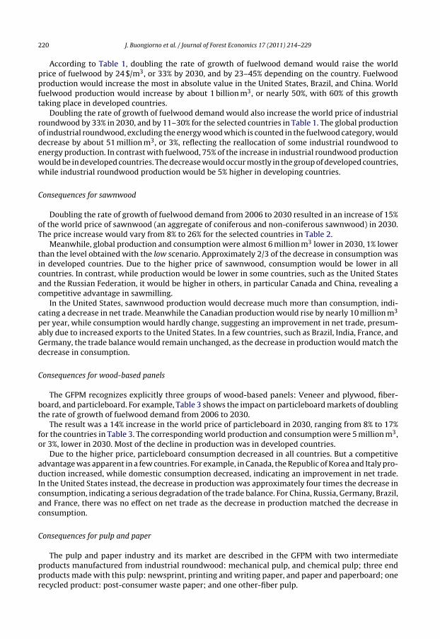
The GFPM recognizes explicitly three groups of wood-based panels: Veneer and plywood, fiber-board, and particleboard. For example, Table 3 shows the impact on particleboard markets of doublingthe rate of growth of fuelwood demand from 2006 to 2030.

The result was a 14% increase in the world price of particleboard in 2030, ranging from 8% to 17%for the countries in Table 3. The corresponding world production and consumption were 5 million m3,or 3%, lower in 2030. Most of the decline in production was in developed countries.

Due to the higher price, particleboard consumption decreased in all countries. But a competitiveadvantage was apparent in a few countries. For example, in Canada, the Republic of Korea and Italy pro-duction increased, while domestic consumption decreased, indicating an improvement in net trade.In the United States instead, the decrease in production was approximately four times the decrease inconsumption, indicating a serious degradation of the trade balance. For China, Russia, Germany, Brazil,and France, there was no effect on net trade as the decrease in production matched the decrease inconsumption.

Consequences for pulp and paper

The pulp and paper industry and its market are described in the GFPM with two intermediateproducts manufactured from industrial roundwood: mechanical pulp, and chemical pulp; three endproducts made with this pulp: newsprint, printing and writing paper, and paper and paperboard; onerecycled product: post-consumer waste paper; and one other-fiber pulp.


Table 2Consequences for sawnwood by region and selected countries.

Effects on

Price$/m3

Production1000 m3

Consumption1000 m3

Africa −1029 −7% −269 −2%Egypt 50 26% −47 −3% −47 −2%Nigeria 56 25% −62 −2% −62 −2%South Africa 25 10% −42 −2% −31 −1%

North/Central America −15,761 −9% −2161 −1%Canada 26 13% 9518 26% −267 −1%Mexico 35 15% −1282 −40% −108 −1%United States of America 31 14% −23,973 −19% −1749 −1%

South America −623 −2% −587 −2%Argentina 36 17% −29 −2% −29 −2%Brazil 37 17% −404 −2% −404 −2%Chile 37 18% −107 −1% −104 −2%

Asia 7909 8% −1240 −1%China 26 11% 7048 28% −388 −1%India 32 12% −231 −1% −231 −1%Indonesia 24 10% −37 −1% −37 −1%Japan 19 8% 300 2% −165 −1%Korea, Republic of 25 10% 92 2% −61 −1%Malaysia 24 11% −45 −1% −45 −1%

Oceania −265 −3% −128 −1%Australia 41 18% −223 −4% −91 −2%New Zealand 24 12% −29 −1% −29 −1%

Europe 3806 2% −1577 −1%EU-25 4383 4% −1270 −1%Austria 25 12% 1115 16% −59 −1%Finland 24 11% 1779 24% −58 −1%France 26 12% −138 −1% −138 −1%Germany 24 12% −213 −1% −213 −1%Italy 30 13% 1052 95% −111 −1%Russian Federation 40 19% −1964 −12% −168 −2%Spain 18 8% 699 16% −54 −1%Sweden 30 15% −1804 −4% −83 −1%United Kingdom 29 13% 2246 56% −133 −1%

Developed, all −10,705 −3% −3942 −1%Developing, all 4743 3% −2020 −1%World 30 15% −5962 −1% −5962 −1%

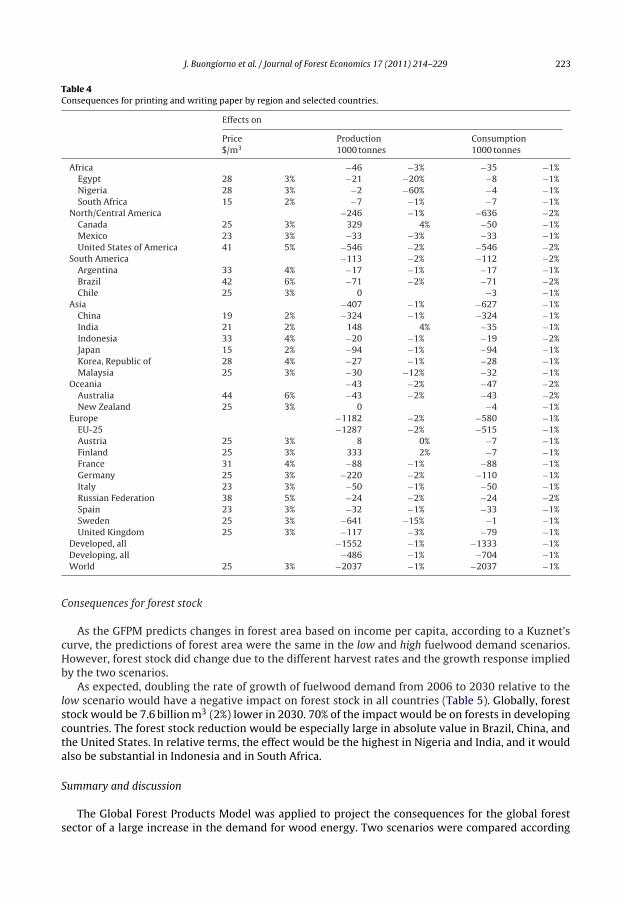
As expected, the magnitude of the effects of higher fuelwood demand diminished with increasedlevels of processing. An example of this, for printing and writing paper, is in Table 4. Doubling therate of growth of fuelwood demand from 2006 to 2030 raised the world price of printing and writingpaper by 3% in 2030, and the price in individual countries by 2–6%. This was much less than the 33%increase of the world price of industrial roundwood (see Table 1), and still less than the 12% increaseof the world price of wood pulp.

The higher price of printing and writing paper led to a decrease in consumption in all countries(Table 4), and a decrease of about 2 million metric tonnes (1%) in world consumption, 80% of it occur-ring in developed countries. The changes in production and consumption for individual countriesrevealed strong differences in comparative advantage. While the decline in production in the UnitedStates, China, Japan, France, and Brazil matched that of consumption, leaving net trade unchanged, theproduction in Sweden and Germany would decrease much more than domestic consumption, witha deterioration of the trade balance. Meanwhile Canada and Finland increased production, added totheir small decrease in domestic consumption meant a large increase in net trade of printing andwriting paper.


Table 3Consequences for particleboard by region and selected countries.

Effects on

Price Production Consumption

$/m3 1000 m3 Dif% 1000 m3


North/Central America −3708 −8% −1711 −4%Canada 26 12% 2837 23% −115 −3%Mexico 32 13% −12 −46% −15 −3%United States of America 36 16% −6529 −18% −1573 −4%

South America −326 −5% −275 −4%Argentina 34 15% −27 −4% −27 −4%Brazil 36 15% −158 −4% −158 −4%Chile 39 18% −84 −9% −35 −5%

Asia 21 0% −841 −3%China 24 9% −436 −3% −437 −3%India 29 10% −7 −3% −6 −3%Indonesia 23 9% −14 −3% −13 −3%Japan 17 7% 133 11% −35 −2%Korea, Republic of 32 13% 393 68% −96 −3%Malaysia 24 11% −12 −5% −1 −4%

Oceania −83 −6% −73 −5%Australia 45 20% −78 −6% −67 −5%New Zealand 24 11% −5 −2% −5 −3%

Europe −897 −2% −2072 −3%EU-25 −449 −1% −1588 −4%Austria 24 11% 241 16% −29 −3%Finland 24 11% 41 12% −8 −3%France 32 14% −142 −3% −142 −4%Germany 24 11% −285 −3% −285 −3%Italy 27 11% 780 27% −118 −3%Russian Federation 35 14% −303 −4% −303 −4%Spain 19 8% −110 −3% −85 −2%Sweden 29 12% −26 −3% −26 −3%United Kingdom 29 12% 253 8% −131 −3%

Developed, all −4593 −4% −3952 −4%Developing, all −445 −1% −1087 −3%World 30 14% −5038 −3% −5039 −3%

Consequences for value added

A standard output of the GFPM is the value added by manufacturing. This is the value of all the out-put minus the cost of the input. In the sawnwood, panels, and pulp sectors it is the value of sawnwoodand panels minus the cost of the industrial roundwood used in making them. In the paper sector, thevalue added is the value of newsprint, printing and writing paper, and other paper and paperboard,minus the cost of wood pulp, recycled paper, and other fiber input.

In this application, no transformation of the fuelwood, harvested in the forest or obtained fromindustry residues, was considered. Therefore, the change in value added was only the change occurringin traditional forest industries (sawnwood, panels, pulp, and paper and paperboard).

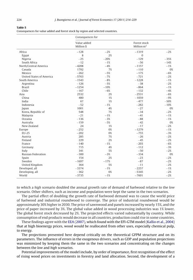
Table 5 shows that, was the rate of growth of fuelwood demand to double from 2006 to 2030,the global value added in traditional industries would decrease by some $3.7 billion, or about 1%,in constant $US of 1997 purchasing power. Most of the decrease would be in developed countries.The largest absolute decrease of value added would occur in the United States, Brazil, and Sweden.However, other countries would gain, in particular Canada, Finland, China, and the Republic of Korea.In several countries the increase in fuelwood demand would have relatively little effect on value added.


Table 4Consequences for printing and writing paper by region and selected countries.

Effects on

Price$/m3

Production1000 tonnes

Consumption1000 tonnes


North/Central America −246 −1% −636 −2%Canada 25 3% 329 4% −50 −1%Mexico 23 3% −33 −3% −33 −1%United States of America 41 5% −546 −2% −546 −2%

South America −113 −2% −112 −2%Argentina 33 4% −17 −1% −17 −1%Brazil 42 6% −71 −2% −71 −2%Chile 25 3% 0 −3 −1%

Asia −407 −1% −627 −1%China 19 2% −324 −1% −324 −1%India 21 2% 148 4% −35 −1%Indonesia 33 4% −20 −1% −19 −2%Japan 15 2% −94 −1% −94 −1%Korea, Republic of 28 4% −27 −1% −28 −1%Malaysia 25 3% −30 −12% −32 −1%

Oceania −43 −2% −47 −2%Australia 44 6% −43 −2% −43 −2%New Zealand 25 3% 0 −4 −1%

Europe −1182 −2% −580 −1%EU-25 −1287 −2% −515 −1%Austria 25 3% 8 0% −7 −1%Finland 25 3% 333 2% −7 −1%France 31 4% −88 −1% −88 −1%Germany 25 3% −220 −2% −110 −1%Italy 23 3% −50 −1% −50 −1%Russian Federation 38 5% −24 −2% −24 −2%Spain 23 3% −32 −1% −33 −1%Sweden 25 3% −641 −15% −1 −1%United Kingdom 25 3% −117 −3% −79 −1%

Developed, all −1552 −1% −1333 −1%Developing, all −486 −1% −704 −1%World 25 3% −2037 −1% −2037 −1%

Consequences for forest stock

As the GFPM predicts changes in forest area based on income per capita, according to a Kuznet’scurve, the predictions of forest area were the same in the low and high fuelwood demand scenarios.However, forest stock did change due to the different harvest rates and the growth response impliedby the two scenarios.

As expected, doubling the rate of growth of fuelwood demand from 2006 to 2030 relative to thelow scenario would have a negative impact on forest stock in all countries (Table 5). Globally, foreststock would be 7.6 billion m3 (2%) lower in 2030. 70% of the impact would be on forests in developingcountries. The forest stock reduction would be especially large in absolute value in Brazil, China, andthe United States. In relative terms, the effect would be the highest in Nigeria and India, and it wouldalso be substantial in Indonesia and in South Africa.

Summary and discussion

The Global Forest Products Model was applied to project the consequences for the global forestsector of a large increase in the demand for wood energy. Two scenarios were compared according


Table 5Consequences for value added and forest stock by region and selected countries.

Consequences for

Value addedMillion $

Forest stockMillion m3

Africa −128 −2% −1319 −2%Egypt 8 2% 0Nigeria −25 −20% −129 −35%South Africa −12 −1% −56 −14%

North/Central America −4208 −4% −1157 −1%Canada 1792 7% −110 0%Mexico −262 −5% −175 −6%United States of America −5763 −7% −721 −2%

South America −1543 −8% −1228 −1%Argentina −126 −5% −38 −2%Brazil −1254 −10% −864 −1%Chile −167 −6% −132 −4%

Asia 2532 2% −2531 −6%China 480 1% −1059 −9%India 67 1% −477 −50%Indonesia −52 −1% −282 −10%Japan 1001 4% −27 0%Korea, Republic of 548 7% −34 −2%Malaysia −21 −1% −41 −1%Oceania −136 −3% −88 −1%Australia −159 −5% −42 0%New Zealand 24 1% −17 −2%

Europe −252 0% −1279 −1%EU-25 −202 0% −755 −3%Austria 285 7% −26 −2%Finland 229 2% −45 −2%France −140 −1% −203 −6%Germany 715 4% −112 −3%Italy 341 5% −50 −2%Russian Federation −300 −3% −334 0%Spain 154 2% −23 −2%Sweden −1697 −17% −87 −2%United Kingdom 364 5% −11 −2%

Developed, all −3374 −1% −2257 −1%Developing, all −362 0% −5345 −2%World −3735 −1% −7601 −2%

to which a high scenario doubled the annual growth rate of demand of fuelwood relative to the lowscenario. Other shifters, such as income and population were kept the same in the two scenarios.

The partial effect of doubling the growth rate of fuelwood demand was to cause the world priceof fuelwood and industrial roundwood to converge. The price of industrial roundwood would beapproximately 30% higher in 2030. The price of sawnwood and panels increased by nearly 15%, and theprice of paper increased by 3%. The global value added in wood processing industries was 1% lower.The global forest stock decreased by 2%. The projected effects varied substantially by country. Whileconsumption of end products would decrease in all countries, production could rise in some countries.

These findings agree with the EEA (2007), which found with the EFI-GTM model (Kallio et al., 2004)that at high bioenergy prices, wood would be reallocated from other uses, especially chemical pulp,to energy.

The projections presented here depend critically on the theoretical GFPM structure and on itsparameters. The influence of errors in the exogenous drivers, such as GDP and population projectionswas minimized by keeping them the same in the two scenarios and concentrating on the changesbetween the low and high scenarios.

Potential improvements of the model include, by order of importance, first recognition of the effectof rising wood prices on investments in forestry and land allocation. Second, the development of a


theory and empirical representation of trade to replace the trade inertia constraints which currentlylimit periodic variations in trade to be similar to those observed historically (Eqs. (6) and (24)). Third,distinguish between hardwoods and softwoods, and between logs and pulpwood. However, in plan-ning such improvements, one should keep in mind the limitation of the data and that simplicity isgenerally preferable for model use, transparency, and application to illusive precision.

Furthermore, although the model projected the consequence of a rise in fuelwood demand on theforestry stock it did not, and cannot yet, describe the structure of this stock, i.e. the size, species, andage of the trees that make it up. Yet, history tells of drastic changes during the industrial revolutionwhen the demand for fuel and charcoal for salt and iron production led to extensive coppice forests(Badré, 1992; Degron, 1995). A similar expansion of mono-specific short-rotation plantations mustbe expected if the highest fuelwood demand considered here were realized. This would have seriousconsequences for the ecological and aesthetic values of forests, which must be considered in addition tothe data presented here, in any serious policy debate on the future role of forests as fonts of bioenergy.

Acknowledgments

The research leading to this paper was supported in part by the USDA Forest Service, SouthernForest Experiment Station. We are grateful to Jeffrey P. Prestemon for his collaboration and reviewcomments. Any remaining error is our sole responsibility.

Appendix A.

The GFPM calculates every year a global equilibrium across countries and products, linked dynam-ically to past equilibriums.

Spatial global equilibrium

Objective functionThe consumer and producer surplus in a given year, for all countries and products (Samuelson,

1952):

max Z =∑

i

∑k

∫ Dik

0

Pik(Dik)dDik −∑

i

∑k

∫ Sik

0

Pik(Sik)dSik

−∑

i

∑k

∫ Yik

0

mik(Yik)dYik −∑

i

∑j

∑k

cijkTijk

(1)

where i,j = country, k = product, P = price in US dollars of constant value, D = final product demand,S = raw material supply, Y = quantity manufactured, m = manufacturing cost, T = quantity transported,and c = cost of transportation, including tariff. All variables refer to a specific year. In making predic-tions, the period between successive equilibria may be multiple years.

End product demand

Dik = D∗ik

(Pik

Pik,−1

)ıik

(2)

where D* = current demand at last period’s price, P−1 = last period’s price, and ı = price elasticity ofdemand.

As shown in the section on market dynamics, below, D* depends on last period’s demand, and thegrowth of GDP in the country. In the base year, D* is equal to the observed base-year consumption,and P−1 is equal to the observed base-year price.

Eqs. (2), (3) and (7) below are approximated by the tangent at the at the point of coordinates D*and P−1. Thus, Eq. (1) is of second degree and the entire equilibrium problem has a quadratic objectivefunction and linear constraints.


Primary product supply

Sik = S∗ik

(Pik

Pik,−1

)�ik

(3)

where S* = current supply at last period’s price and � = price elasticity of supply. As shown in the sectionon market dynamics, below, S* depends on the last period’s supply and on exogenous or endogenoussupply shifters. In the base year, S* is equal to the base-year supply, and P−1 is equal to the observedbase year price.

Total wood supplySi = Si,r + Sin + �iSif (4)

r = industrial roundwood, n = other industrial roundwood, f = fuelwood, � = fraction of fuelwood thatcomes from the forest.

Si ≤ Ii

Ii = forest stock.

Material balance∑j

Tjik + Sik + Yik − Dik −∑

n

aiknYin −∑

j

Tijk = 0 ∀i, k (5)

where aikn = input of product k per unit of product n.In addition, by-products, which result from the production of a manufactured commodity satisfy

the constraint:

Yil − biklYik = 0 ∀i, k, l

where bikl is the amount of by-product l that can be recovered per unit of production of manufacturedcommodity k.

Trade inertiaTL

ijk ≤ Tijk ≤ TUijk (6)

where the superscripts L and U refer to a lower bound, and upper bound, respectively.

PricesThe shadow prices of the material balance constraints (5) give the market-clearing prices for each

commodity and country.

Manufacturing costManufacturing is represented by activity analysis, with input–output coefficients and a manufac-

turing cost. The manufacturing cost is the marginal cost of the inputs not recognized explicitly by themodel (labor, energy, capital, etc.);

m = m∗ik

(Yik

Yik,−1

)sik

(7)

where m* = current manufacturing cost, at last period’s output and s = elasticity of manufacturing costwith respect to output.

As shown in the next section, m* depends on the last period’s quantity manufactured and on theexogenous rate of change of manufacturing cost. In the base year, m* is equal to the observed base-yearmanufacturing cost and Yik,−1 is equal to the observed base-year quantity manufactured.


Transport costThe transport cost for commodity k from country i to country j in any given year is:

cijk = fijk + tIjk(fijk + Pik,−1) (8)

where c = international transport cost,1 per unit of volume, f = freight cost, per unit of volume,tI = import ad-valorem tariff, and P−1 = last period’s equilibrium export price computed endogenouslyby the model. In the base year, P−1 is equal to the observed base-year price.

Market dynamics2

All periodic exponential rates of change, rp, are defined by the annual exponential rate of change,ra, as:

rp = (1 + ra)p − 1 (9)

where p is the length of a period, in years.All periodic linear changes, �vp are defined by the corresponding annual linear change, �va, as:

�vp = p�va (10)

Shifts of demandD∗ = D−1(1 + ˛ygy) (11)

gy = GDP periodic growth rate, ˛ = elasticity.

Shifts of supplyFor industrial roundwood and fuelwood:

S∗ = S−1(1 + ˇIgI + ˇy′ gy′ ) for k = r, n, f (12)

where gI = periodic rate of change of forest stock (endogenous, see below), gy′ = periodic rate of changeof GDP per capita, and ˇ = elasticity.

For waste paper and other fiber pulp:

S∗ = S−1(1 + ˇygy) (13)

Changes in forest area and forest stockA = (1 + ga)A−1 (14)

where A = forest area, and ga = periodic rate of forest area change based on the period length, p, Eq. (9)and the annual rate of forest area change, gaa, defined by an environmental Kuznet’s curve (Turneret al., 2006):

gaa = ˛0 + ˛1y′ + ˛2y′2 for y′ ⇐ y′∗, else gaa = 0 (15)

where for each country, ˛0 is calibrated so that in the base year the observed gaa is equal to the gaa

projected with (15) given the income per capita y′.y′ = income per capita, projected from:

y′ = (1 + gy′ )y′−1 (16)

y′* is defined by

gaa = ˛0 + ˛1y′∗ + ˛2y′∗2 = 0 and y′∗ >−˛1

2˛2(17)

1 Domestic transport cost is reflected by the supply Eq. (3) and the manufacturing cost (7).2 Unless otherwise indicated, variables refer to one country, one commodity, and one year. Rates of change refer to a multi-year

period.


Forest stock evolves over time according to a growth-drain equation:

I = I−1 + G−1 − pS−1 (18)

where G = (ga + gu + g∗u)I is the periodic change of forest stock without harvest, gu = periodic rate of

forest growth on a given area, without harvest, and gu* = adjustment of periodic rate of forest growthon a given area, without harvest. The last is exogenous, for example to represent the effect of invasivespecies, or of climate change.

The periodic rate of forest growth, gu, is based on the annual rate of forest growth, gua, defined by:

gua = �0

(I

A

)�

(19)

where � is negative, so that gua decreases with stock per unit area. For each country, �0 is calibratedso that in the base year the observed gua is equal to the gua predicted by (19) given the stock per unitarea, I/A.

The periodic rate of change of forest stock net of harvest, used in Eq. (12) is then:

gI = I − I−1

I−1(20)

Changes in manufacturing coefficients and costsThe input–output coefficients a in Eq. (5), may change exogenously over time, for example to reflect

increasing use of recycled paper in paper manufacturing:

a = a−1 + �a (21)

where �a = periodic change in input–output coefficient.The manufacturing cost function shifts exogenously over time:

m∗ = m−1(1 + gm) (22)

where gm = the exogenous rate of periodic change in manufacturing cost.

Changes in freight cost and tariffThe freight cost and the import tariffs in Eq. (8) may change exogenously over time:

f = f−1 + �f, t = t−1 + �t (23)

where �f and �t are periodic changes in freight cost and tariff, respectively.

Changes in trade inertia boundsTL = T−1(1 − ε)p

TU = T−1(1 − ε)p (24)

ε = absolute value of maximum annual relative change in trade flow (exogenous, based on historicaldata).

Linear approximation of demand, supply, manufacturing cost

For example, consider a demand equation such as (2). Omitting the subscripts for region andproduct, the inverse demand equation in any given year is:

P = P−1

(D

D∗

)1/�

The linear approximation is:

P = a + bD with a = P−1 − bD∗ and b = P−1

�D∗ for D∗ > 1, else b = P−1

�(25)

b = 0 if � = 0. The same method is used for the supply, and the manufacturing cost equations.


References

Alcamo, J., van Vuuren, D., Ringer, C., Cramer, W., Masui, T., Alder, J., Schulze, K., 2005. Changes in nature’s balance sheet:model-based estimates of future worldwide ecosystem services. Ecology and Society 10 (2), 1–19.

Badré, L., 1992. Les forêts et l’industrie en Lorraine à la fin du XVIIIe siècle. Revue Forestière Francaise 44 (4), 365–369.Bright, R.M., Stromman, A.H., Hawkins, T.R., 2010. Environmental assessment of wood-based biofuel production and consump-

tion scenarios in Norway. Journal of Industrial Ecology 14 (3), 422–439.Buongiorno, J., Liu, C.S., Turner, J., 2001. Estimating international wood and fiber utilization accounts in the presence of mea-

surement errors. Journal of Forest Economics 7 (2), 101–124.Buongiorno, J., Zhu, S., Zhang, D., Turner, J., Tomberlin, D., 2003. The Global Forest Products Model: Structure, Estimation, and

Applications. Academic Press/Elsevier, San Diego.Day, R.H., 1973. Recursive programming models: a brief introduction. In: Judge, G.G., Takayama, T. (Eds.), Studies in Economic

Planning Over Space and Time: Contributions to Economic Analysis. American Elsevier, New York, pp. 329–344.Degron, R., 1995. Historique de la forêt du Romesberg: Une forêt de Lorraine sous l’empire des salines. Revue Forestière Francaise

47 (5), 590–597.European Energy Agency (EEA), 2007. Environmentally Compatible Bio-energy Potential from European Forests. Avail-

able from: biodiversity-chm.eea.europa.eu/information/database/forests/EEA Bio Energy 10-01-2007 low.pdf/download(accessed 18.06.09.).

FAO (Food and Agriculture Organization of the United Nations), 2006. Global Forest Resources Assessment 2005. ProgressTowards Sustainable Management. FAO Forestry Paper 147. Food and Agriculture Organization of the United Nations, Rome.

FAO (Food and Agriculture Organization of the United Nations), 2008a. FAOSTAT Forestry Data 1961–2006. Available from:http://faostat.fao.org/site/626/default.aspx#ancor (accessed 19.06.09.).

FAO (Food and Agriculture Organization of the United Nations), 2008b. FAO Yearbook, Forest Products, 2002–2006. Food andAgriculture Organization of the United Nations, Rome.

Intergovernmental Panel on Climate Change (IPPC), 2001. Climate Change 2001: Impacts, Adaptation, and Vulnerability. Cam-bridge University Press, Cambridge, UK.

Kallio, A.M.I., Moiseyev, A., Solberg, B., 2004. The Global Forest Sector Model EFI-GTM. The Model Structure. European ForestInstitute, Joensuu, EFI Internal Report 15.

Kirilenko, A.P., Sedjo, R.A., 2007. Climate change impacts on forestry. Proceedings of the National Academy of Sciences of theUnited States of America 104 (50), 19697–19702.

Kramp, A., Ince, P., 2010. The US Forest Products Module (USFPM): Forest Sector Modeling using GFPM with global wood energyand climate change scenarios. In: Paper Presented at International Workshop, Nancy, France, 3–4 June.

Nakicenovic, N., Davidson, O., Davis, G., Grübler, A., Kram, T., Lebre La Rovere, E., Metz, B., Morita, T., Pepper, W., Pitcher, H.,Sankovski, A., Shukla, P., Swart, R., Watson, R., Zhou, D., 2000. Special Report on Emissions Scenarios: A Special Report ofWorking Group III of the Intergovernmental Panel on Climate Change. Cambridge University Press, Cambridge, UK, 599 pp.Available from: http://www.grida.no/climate/ipcc/emission/index.htm.

Perez-Garcia, J., Joyce, L.A., McGuire, A.D., Xiao, X., 2002. Impacts of climate change on the global forest sector. Climatic Change54, 439–461.

Raunikar, R., Buongiorno, J., Turner, J.A., Zhu, S., 2010. Global outlook for wood and forests with the bioenergy demand impliedby scenarios of the intergovernmental panel on climate change. Forest Policy and Economics 12, 48–56.

Samuelson, P.A., 1952. Spatial price equilibrium and linear programming. American Economic Review 42 (3), 283–303.Simangunsong, B.C.H., Buongiorno, J., 2001. International demand equations for forest products: a comparison of methods.

Scandinavian Journal of Forest Research 16, 155–172.Sohngen, B., Mendelsohn, R., 1998. Valuing the impact of large-scale ecological change in a market: the effect of climate change

on U.S. timber. American Economic Review 88 (4), 689–710.Stennes, B., Niquidet, K., Kooten, G.C.van., 2010. Implications of expanding bioenergy production from wood in British Columbia:

an application of a regional wood fibre allocation model. Forest Science 56, 366–378.Turner, J.A., Buongiorno, J., Zhu, S., 2006. An economic model of international wood supply, forest stock and forest area change.

Scandinavian Journal of Forest Research 21, 73–86.USDA Forest Service, 2008. Future Scenarios and Assumptions for the 2010 Resources Planning Act (RPA) Assessment. General

Technical Report WO-(Draft). U.S. Department of Agriculture, Forest Service, Washington Office, Washington, DC.World Bank, 2008. World Bank Development Indicators. Available from: http://ddpext.worldbank.org/ext/DDPQQ/member.do?

method=getMembers&userid=1&queryId=135.Zhu, S., Buongiorno, J., Turner, J.A., Li, R., 2009. Calibrating and Updating the Global Forest Products Model. Staff Paper Series #

67. Department of Forest Ecology and Management, University of Wisconsin, Madison, WI.

http://faostat.fao.org/site/626/default.aspx

http://www.grida.no/climate/ipcc/emission/index.htm

Documents

Journal of Forest Economics - Southern Research · J. Buongiorno et al. / Journal of Forest Economics 17 (2011) 214–229 219 by 2030. The price of sawnwood would approximately follow