Contents lists available at ScienceDirect

Journal of Financial Economics

Journal of Financial Economics 99 (2011) 672–692

0304-40

doi:10.1

$ We

Univers

particip

(especia

Rotterd

Nick Bo

Centre

fully ac

Centre a

This art

INQUIR

circulat

predictan Corr

fax: +4

E-m

journal homepage: www.elsevier.com/locate/jfec

Hedge funds, managerial skill, and macroeconomic variables$

Doron Avramov a,b, Robert Kosowski c, Narayan Y. Naik d,n, Melvyn Teo e

a Hebrew University of Jerusalem, Israelb R.H. Smith School of Business, University of Maryland, MD, USAc Imperial College Business School, Imperial College London, UKd London Business School, UKe Singapore Management University, Singapore

a r t i c l e i n f o

Article history:

Received 25 March 2009

Received in revised form

13 January 2010

Accepted 13 February 2010

JEL classification:

G11

G12

G14

G23

Keywords:

Hedge funds

Predictability

Managerial skills

Macroeconomic variables

5X/$ - see front matter & 2010 Elsevier B.V.

016/j.jfineco.2010.10.003

thank an anonymous referee, seminar part

ity and the Interdisciplinary Center, Herzliya

ants at the 2008 American Finance Ass

lly Luis Viceira, the discussant), the 2007 E

am Conference on Professional Asset Mana

llen, the discussant), and the 2006 Imperial C

Conference for valuable comments and sugg

knowledge financial support from the BNP P

t the Singapore Management University and

icle represents the views of the authors and n

E. The usual disclaimer applies. This pap

ed under the title ‘‘Investing in hedge funds

ble’’.

esponding author. Tel.: +44 20 7262 5050;

4 20 7724 3317.

ail address: nnaik@london.edu (N.Y. Naik).

a b s t r a c t

This paper evaluates hedge fund performance through portfolio strategies that

incorporate predictability based on macroeconomic variables. Incorporating predict-

ability substantially improves out-of-sample performance for the entire universe of

hedge funds as well as for various investment styles. While we also allow for

predictability in fund risk loadings and benchmark returns, the major source of

investment profitability is predictability in managerial skills. In particular, long-only

strategies that incorporate predictability in managerial skills outperform their Fung and

Hsieh (2004) benchmarks by over 17% per year. The economic value of predictability

obtains for different rebalancing horizons and alternative benchmark models. It is also

robust to adjustments for backfill bias, incubation bias, illiquidity, fund termination, and

style composition.

& 2010 Elsevier B.V. All rights reserved.

1. Introduction

The year 2008 was a difficult one for hedge funds.Many hitherto successful hedge fund managers who had

All rights reserved.

icipants at Bar Ilan

, Israel, as well as

ociation meetings

rasmus University

gement (especially

ollege Hedge Fund

estions. We grate-

aribas Hedge Fund

from INQUIRE, UK.

ot of BNP Paribas or

er was previously

when returns are

consistently delivered stellar returns were hit withsignificant losses. Investors long conditioned to expecthigh alpha from such financial cognoscenti were sorelydisappointed and withdrew funds en masse. For example,despite illustrious multi-year track records, both KennethGriffin of Citadel Investment Group and Daniel Ziff of Och-Ziff Capital Management posted significant losses in 2008.As a result of Citadel’s poor performance, Griffin wasforced to waive management fees and erect gates tostanch the massive wave of redemptions.1 Have hedgefund managers lost their edge or are they simply victims

1 See, for example, ‘‘Hedge Fund Selling Puts New Stress on Market,’’

The Wall Street Journal, 7 November 2008, and ‘‘Crisis on Wall Street:

Citadel Freezes Its Funds Through March,’’ The Wall Street Journal, 13

December 2008. Another star fund manager who suffered losses in 2008

is James Simons whose Renaissance Institutional Futures Fund and

Renaissance Institutional Equities Fund slumped 12% and 16%, respec-

tively. See ‘‘Renaissance Waives Fees on Fund That Gave Up 12%,’’ The

Wall Street Journal, 5 January 2009.

D. Avramov et al. / Journal of Financial Economics 99 (2011) 672–692 673

of the prevailing market conditions? How should fundmanagers be evaluated given that their performancecould be affected by macroeconomic factors? The factthat some investment styles such as global macro andmanaged futures thrive under the volatile conditionswhile others do not, suggests that conditioning on theeconomy could be important when evaluating hedge fundperformance.2

In this paper, we confront these issues by analyzing theperformance of portfolio strategies that invest in hedgefunds. These strategies exploit predictability, based onmacroeconomic variables, in fund manager asset selectionand benchmark timing skills, hedge fund risk loadings,and benchmark returns. By examining the out-of-sampleinvestment opportunity set, we show that allowing forpredictability based on macroeconomic variables isimportant in ex ante identifying subgroups of hedgefunds that deliver significant outperformance. Our analy-sis leverages on the Bayesian framework proposed byAvramov and Wermers (2006), who study the perfor-mance of optimal portfolios of equity mutual funds thatutilize conditional return predictability. In particular, theyfind that long-only strategies that incorporate predict-ability in managerial skills outperform their Fama andFrench (1993) and momentum benchmarks by 2–4% peryear by timing industries over the business cycle and byan additional 3–6% per year by choosing funds thatoutperform their industry benchmarks.

We argue that the Avramov and Wermers frameworkis even more relevant to the study of hedge fundperformance because hedge funds engage in a muchmore diverse set of strategies than do mutual funds.Hedge funds trade in different markets, with differentsecurities, and at different frequencies. They could employleverage, complex derivatives, and short-selling. Themultitude of hedge fund strategies include global macro,managed futures, convertible arbitrage, short selling,statistical arbitrage, equity long/short, and distresseddebt. Anecdotal evidence suggests that the success ofthese strategies hinges on the behavior of variouseconomic indicators such as the credit spread andvolatility.3 In contrast, the mutual fund universe is muchless diverse. Equity mutual funds, for instance, differmainly according to the style of securities that they investin (e.g., small cap versus large cap and value versusgrowth). Therefore, macroeconomic variables are likely tobe more important for explaining the cross-sectionalvariation in managerial skill for hedge funds.

To adjust for risk, we employ the methodology of Fungand Hsieh (2004). Fung and Hsieh (1999, 2000, 2001),Mitchell and Pulvino (2001), and Agarwal and Naik (2004)

2 According to the 2008 Hedge Fund Research report, the average

global macro fund gained 4.84% in 2008. In contrast, the average equity

long/short fund lost 26.28% over the same period. Indeed, some macro-

focused hedge fund families took advantage of the volatile market in

2008 to raise capital and set up new funds. See ‘‘Brevan Howard to Raise

Dollars 500m with New Fund,’’ The Financial Times, 6 March 2008.3 For example, Lowenstein (2000) provides a vivid account of how a

flight to quality, brought about by the Russian ruble default, caused

Long-Term Capital Management to simultaneously lose money on its

risk arbitrage, relative value, and fixed income arbitrage trades.

show that hedge fund returns relate to conventional assetclass returns and option-based strategy returns. Buildingon this, Fung and Hsieh (2004) show that their parsimo-nious asset-based style factor model can explain up to 80%of the variation in global hedge fund portfolio returns. TheFung and Hsieh (2004) factor model includes bond factorsderived from changes in term and credit spreads. Weadjust these factors appropriately for duration so thatthey represent returns on traded portfolios. In sensitivitytests, to account for hedge funds’ exposure to emergingmarket equities, distress risk, stock momentum, andilliquidity, we augment the Fung and Hsieh (2004) modelwith the MSCI emerging markets index excess return, theFama and French (1993) high-minus-low (HML) book-to-market factor, the Jegadeesh and Titman (1993) momen-tum factor, and the Pastor and Stambaugh (2003) liquidityfactor, respectively. We also redo the analysis usingoption-based factors from the Agarwal and Naik (2004)model to ensure that our results are not artifacts of therisk model we use.

Our results suggest that fund manager performanceshould be evaluated conditional on various macroeco-nomic variables. Allowing for predictability in managerialskills based on macroeconomic variables, especially thedefault spread and some measure of volatility, is impor-tant for forming optimal portfolios that outperform expost. Between 1997 and 2008, an investor who allows forpredictability in hedge fund alpha, beta, and benchmarkreturns can earn a Fung and Hsieh (2004) alpha of 17.42%per annum out-of-sample. This is over 10% per annumhigher than that earned by an investor who does not allowfor predictability and over 13% per annum higher thanthat earned by an investor who completely excludes allpredictability and the possibility of managerial skills. Incontrast, the naıve strategy that invests in the top 10% offunds based on past three-year alpha achieves an ex postalpha of only 5.25% per year. The macroeconomicvariables we condition on include the credit spread andthe Chicago Board Options Exchange (CBOE) volatilityindex or the VIX. Our findings about the economic value ofpredictability in hedge fund returns are robust to adjust-ments for backfill and incubation bias (Fung and Hsieh,2004), and illiquidity-induced serial correlation in fundreturns (Getmansky, Lo, and Makarov, 2004). The resultsalso remain qualitatively unchanged when we allow forrealistic rebalancing horizons or remove funds that arelikely to be closed to new investments.

We find that strategies that incorporate predictability inmanagerial skills significantly outperform other strategiesmost within the following broad investment style cate-gories: equity long/short, directional trader, security selec-tion, and multi-process. They are less successful withinrelative value and funds of funds. One view is that bydiversifying across various hedge funds, funds of fundsbecome less dependent on economic conditions. Theoptimal portfolios of hedge funds that allow for predict-ability in managerial skills do differ somewhat from theother portfolios in terms of investment style composition.Given the within-style results, it is not surprising that thewinning strategies also tend to contain a larger proportionof funds from the directional trader and security selection

D. Avramov et al. / Journal of Financial Economics 99 (2011) 672–692674

styles in which conditioning on managerial skills generatesthe greatest payoffs. Conversely, they also tend to containfewer funds from the relative value style in which thepayoffs from conditioning on managerial skills are lower.Nonetheless, a style-based decomposition of the optimalportfolio strategy reveals that only a small part of its relativeperformance can be explained by the strategy’s allocation toinvestment styles. In particular, a portfolio that mimics theoptimal portfolio’s allocations to fund styles delivers analpha of 5.90% per annum. The alpha spread between theoptimal portfolio and this style-mimicking portfolio is11.52% per annum, which is still 13.39% per annum higherthan the style-adjusted alpha spreads for the strategy thatdoes not allow for predictability and the possibility ofmanagerial skills. Hence, the outperformance of the pre-dictability based strategy cannot be simply explained by thepotentially time-varying style composition of the optimallyselected fund portfolio.

What is the economic importance of conditioningmanagerial skills on macroeconomic variables? We findthat the optimal strategy that allows for predictability inmanagerial skills performed decently during thebull market of the 1990s, reasonably well during the2001–2002 market downturn, and exceptionally wellduring the stock market run up from 2003–2007. Aninitial investment of $10,000 in this optimal portfoliotranslates to over $110,000 at the end of our sampleperiod (1997–2008). In contrast, the same initial invest-ment in the S&P 500, in the top 10% of hedge funds basedon past three-year alpha, or in the strategy that does notallow for predictability and managerial skill, all yield lessthan $30,000.4 Some of the impressive returns generatedby the optimal strategy in 2003, 2006, and 2007 can betraced to positions in hedge funds operating in emergingmarkets. However, as we show in our analysis, thestrategy outperforms not because of its exposure tospecific geographical regions but rather because it selectsthe right funds investing within those regions that deliveralpha in the out-of-sample period. This holds true evenafter controlling for time-varying exposure to the MSCIemerging markets index.

The findings in this paper resonate with the literature onthe value of active management in the hedge fund industry.Malkiel and Saha (2005) report that, after adjusting forvarious hedge fund database biases, on average hedge fundssignificantly under-perform their benchmarks. Brown,Goetzmann, and Ibbotson (1999) show that annual hedgefund returns do not persist. Fuelling the debate, Getmansky,Lo, and Makarov (2004) argue that whatever persistence atquarterly horizons, shown by Agarwal and Naik (2000) andothers in hedge funds, can be traced to illiquidity-inducedserial correlation in fund returns. Recent papers offer moresanguine evidence on the existence of active managementskills amongst hedge fund managers. Fung, Hsieh, Naik, andRamadorai (2008) split their sample of funds of funds intohave-alpha and beta-only funds. They find that have-alpha

4 A comparison of the optimal strategy portfolio with just the S&P

500 might not be very insightful as hedge funds, by virtue of their low

market betas, tend to outperform stocks in down markets. Therefore, we

include other portfolios of hedge funds in the analysis.

funds exhibit better survival rates and experience steadierinflows than do beta-only funds. Kosowski, Naik, and Teo(2007) demonstrate, using a bootstrap approach, that thealpha of the top hedge funds cannot be explained by luck orsample variability. They also show that after overcoming theshort sample problem inherent in hedge fund data with theBayesian approach of Pastor and Stambaugh (2002), hedgefund risk-adjusted performance persists at annual horizons.Finally, Aggarwal and Jorion (2010) show using a novelevent time approach that emerging funds and managersoutperform other hedge funds and that strong earlyperformance can persist up to five years.

We show that conditioning on macroeconomicvariables is important in capturing fund managerial skill.The out-of-sample performance of the optimal portfolio thatallows for predictability, based on macroeconomic variables,in managerial skills is substantially higher than that for thetop decile of funds sorted on the Kosowski, Naik, and Teo(2007) Bayesian alpha or on Ordinary Least Squares (OLS)alpha. We believe that our methodology improves perfor-mance by ex ante selecting good managers who wereunfortunate victims of economic circumstance while avoid-ing bad managers who were lucky beneficiaries of economiccircumstance. For example, in 2003, the optimal strategythat allows for predictability and managerial skill placedlarge weights on two funds: an emerging markets fund anda long bias fund. Based on their past three-year OLS alpha,these funds were not very impressive. Yet in the out-of-sample period (i.e., 2003), their returns easily surpassedmost of the top funds in our sample ranked by pastthree-year OLS alpha. One caveat is that the optimal strategyis fairly concentrated in small to mid-size hedge funds.On average, there are nine funds in the portfolio whilethe median fund assets under management (AUM) is$187 million. Given the capacity constraints (Berk andGreen, 2004) that hedge funds face, this suggests that asignificant amount of capital cannot be put to work in thisstrategy.

The rest of the paper is structured as follows. Section 2reviews the methodology used in the analysis, and Section3 describes the data. Section 4 presents the empiricalresults. Section 5 concludes.

2. Methodology

We assess the economic significance of predictabilityin hedge fund returns as well as the overall value of activehedge fund management.5 Our experiments are based onthe perspectives of Bayesian optimizing investors whodiffer with respect to their beliefs about the potential forhedge fund managers to possess asset selection skills andbenchmark timing abilities. The investors differ in theirviews about the parameters governing the followinghedge fund return generating model:

rit ¼ ai0þaui1zt�1þbui0ftþbui1ðft � zt�1Þþuit , ð1Þ

5 See Avramov and Wermers (2006) for a more detailed discussion

of the methodology.

D. Avramov et al. / Journal of Financial Economics 99 (2011) 672–692 675

ft ¼ af þAf zt�1þuft , ð2Þ

zt ¼ azþAzzt�1þuzt , ð3Þ

where rit is the month-t hedge fund return in excess ofthe risk free rate, zt�1 contains M business cycle variablesobserved at end of month t�1, ft is a set of K zero-costbenchmarks typically used to assess hedge fund perfor-mance, bi0(bi1) is the fixed (time-varying) component offund risk loadings, and uit is an idiosyncratic eventassumed to be uncorrelated across funds and throughtime. We assume that this residual is normally distributedwith zero mean and variance equal to ci.

Two potential sources of timing-related hedge fundreturns are correlated with public information. First, fundrisk-loadings could be predictable. This predictabilitycould stem from changing asset level risk loadings, flowsinto the funds, or manager timing of the benchmarks.Second, the benchmarks, which are return spreads, couldbe predictable. Such predictability is captured throughthe predictive regression in Eq. (2). Because both of thesetiming components can be easily replicated by anyinvestor, we do not consider them to be based onmanagerial skill. Instead, the expression for managerialskill is ai0+ai1

0zt�1 which captures benchmark timing andasset selection skills that exploit only the privateinformation possessed by a fund manager. This privateinformation can be correlated with the business cycle, ascaptured by the predictive variables. This is what we showin the empirical results.

Overall, the model for hedge fund returns described byEqs. (1)–(3) captures potential predictability in manage-rial skills ðai1a0Þ, hedge fund risk loadings ðbi1a0Þ, andbenchmark returns ðAfa0Þ. We now introduce ourinvestors, who differ in their views about the existenceof manager skills in timing the benchmarks and inselecting securities.

The first investor is the dogmatist who rules out anypotential for fixed or time varying manager skill. Thedogmatist believes that a fund manager provides noperformance through benchmark timing or asset selectionskills and that expenses and trading costs are a dead-weight loss to investors. We consider two types ofdogmatists. The no-predictability dogmatist (ND) rulesout predictability and sets the parameters bi1 and Af inEqs. (1) and (2) equal to zero. The predictability dogmatist(PD) believes that hedge fund returns are predictablebased on observable business cycle variables. We furtherpartition the PD investor into two types. The PD-1investor believes that fund risk loadings are predictable(i.e., bi1 is allowed to be nonzero), and the PD-2 investorbelieves that fund risk loadings and benchmark returnsare predictable (i.e., both bi1 and Af are allowed to benonzero).

The second investor is the skeptic who harbors moremoderate views on the possibility of active managementskills. The skeptic believes that some fund managers canbeat their benchmarks, though her beliefs about over-performance or under-performance are bounded, as weformalize below. As with the dogmatist, we also considertwo types of skeptics: the no-predictability skeptic (NS)

and the predictability skeptic (PS). The former believesthat macroeconomic variables should be ignored; thelatter believes that fund risk loadings, benchmark returns,and even managerial skills are predictable based onchanging macroeconomic conditions. For the NS investor,ai1 equals zero with probability one and ai0 is normallydistributed with a mean equal to zero and a standarddeviation equal to 1%.

The third investor is the agnostic who allows formanagerial skills to exist but has completely diffuse priorbeliefs about the existence and level of skills. Specifically,the skill level ai0þaui1zt�1 has a mean of zero andunbounded standard deviation. As with the other inves-tors, we further subdivide the agnostic into the nopredictability agnostic (NA) and the predictabilityagnostic (PA).

Overall, we consider 13 hedge fund investors: threedogmatists, five sceptics, and five agnostics. Table 1summarizes the different investor types and the beliefsthey hold. For each of these 13 investors, we form optimalportfolios of hedge funds. The time-t investment universeis made up of Nt firms, with Nt varying over time as fundsenter and leave the sample through closures andterminations. Each investor type maximizes the condi-tional expected value of the following quadratic function:

UðWt ,Rp,tþ1,at ,btÞ ¼ atþWtRp,tþ1�bt

2W2

t R2p,tþ1, ð5Þ

where Wt denotes wealth at time t, bt is related to the riskaversion coefficient, and Rp,tþ1 is the realized excessreturn on the optimal portfolio of mutual funds computedas Rp,tþ1 ¼ 1þrftþwutrtþ1, with rft denoting the risk freerate, rtþ1 denoting the vector of excess fund returns, andwt denoting the vector of optimal allocations tohedge funds.

By taking conditional expectations on both sides ofEq. (5), letting gt ¼ ðbtWtÞ=ð1�btWtÞ be the relative risk-aversion parameter, and letting Kt ¼ ½Rtþmtmut��1, wheremt and Rt are the mean vector and covariance matrix offuture fund returns, yields the following optimization:

w�t ¼ argmaxwt

wutmt�1

2ð1=gt�rftÞwutK

�1t wt

� �: ð6Þ

We derive optimal portfolios of hedge funds bymaximizing Eq. (6) constrained to preclude short-sellingand leveraging. In forming optimal portfolios, we replacemt and St in Eq. (6) by the mean and variance of theBayesian predictive distribution

pðrtþ19Dt ,IÞ ¼

ZY

pðrtþ19Dt ,Y,IÞpðY9Dt ,IÞdY, ð7Þ

where Dt denotes the data (hedge fund returns, bench-mark returns, and predictive variables) observed up toand including time t, Y is the set of parameterscharacterizing the processes in Eqs. (1)–(3), p Y9Dt

� �is

the posterior density of Y, and I denotes the investor type(13 investors are considered). For each investor type, themean and variance of the predictive distribution obeyanalytic reduced form expressions and are displayed inAvramov and Wermers (2006). Such expected utility

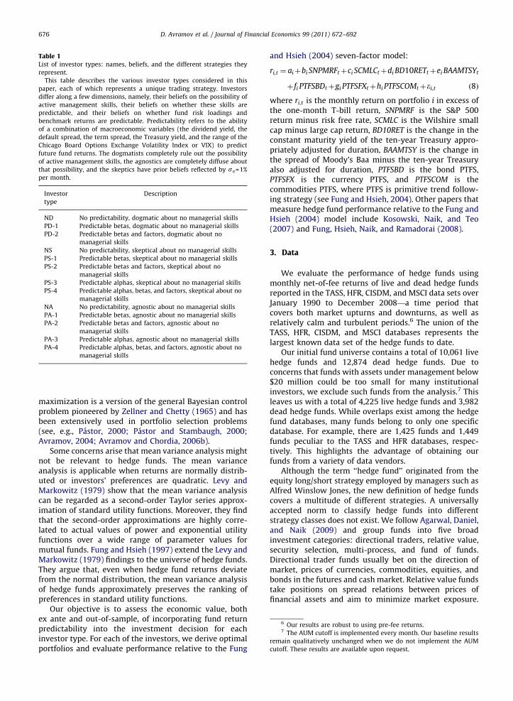
Table 1List of investor types: names, beliefs, and the different strategies they

represent.

This table describes the various investor types considered in this

paper, each of which represents a unique trading strategy. Investors

differ along a few dimensions, namely, their beliefs on the possibility of

active management skills, their beliefs on whether these skills are

predictable, and their beliefs on whether fund risk loadings and

benchmark returns are predictable. Predictability refers to the ability

of a combination of macroeconomic variables (the dividend yield, the

default spread, the term spread, the Treasury yield, and the range of the

Chicago Board Options Exchange Volatility Index or VIX) to predict

future fund returns. The dogmatists completely rule out the possibility

of active management skills, the agnostics are completely diffuse about

that possibility, and the skeptics have prior beliefs reflected by sa=1%

per month.

Investor

type

Description

ND No predictability, dogmatic about no managerial skills

PD-1 Predictable betas, dogmatic about no managerial skills

PD-2 Predictable betas and factors, dogmatic about no

managerial skills

NS No predictability, skeptical about no managerial skills

PS-1 Predictable betas, skeptical about no managerial skills

PS-2 Predictable betas and factors, skeptical about no

managerial skills

PS-3 Predictable alphas, skeptical about no managerial skills

PS-4 Predictable alphas, betas, and factors, skeptical about no

managerial skills

NA No predictability, agnostic about no managerial skills

PA-1 Predictable betas, agnostic about no managerial skills

PA-2 Predictable betas and factors, agnostic about no

managerial skills

PA-3 Predictable alphas, agnostic about no managerial skills

PA-4 Predictable alphas, betas, and factors, agnostic about no

managerial skills

6 Our results are robust to using pre-fee returns.7 The AUM cutoff is implemented every month. Our baseline results

remain qualitatively unchanged when we do not implement the AUM

cutoff. These results are available upon request.

D. Avramov et al. / Journal of Financial Economics 99 (2011) 672–692676

maximization is a version of the general Bayesian controlproblem pioneered by Zellner and Chetty (1965) and hasbeen extensively used in portfolio selection problems(see, e.g., Pastor, 2000; Pastor and Stambaugh, 2000;Avramov, 2004; Avramov and Chordia, 2006b).

Some concerns arise that mean variance analysis mightnot be relevant to hedge funds. The mean varianceanalysis is applicable when returns are normally distrib-uted or investors’ preferences are quadratic. Levy andMarkowitz (1979) show that the mean variance analysiscan be regarded as a second-order Taylor series approx-imation of standard utility functions. Moreover, they findthat the second-order approximations are highly corre-lated to actual values of power and exponential utilityfunctions over a wide range of parameter values formutual funds. Fung and Hsieh (1997) extend the Levy andMarkowitz (1979) findings to the universe of hedge funds.They argue that, even when hedge fund returns deviatefrom the normal distribution, the mean variance analysisof hedge funds approximately preserves the ranking ofpreferences in standard utility functions.

Our objective is to assess the economic value, bothex ante and out-of-sample, of incorporating fund returnpredictability into the investment decision for eachinvestor type. For each of the investors, we derive optimalportfolios and evaluate performance relative to the Fung

and Hsieh (2004) seven-factor model:

ri,t ¼ aiþbi SNPMRFtþci SCMLCtþdi BD10RETtþei BAAMTSYt

þ fi PTFSBDtþgi PTFSFXtþhi PTFSCOMtþei,t ð8Þ

where ri,t is the monthly return on portfolio i in excess ofthe one-month T-bill return, SNPMRF is the S&P 500return minus risk free rate, SCMLC is the Wilshire smallcap minus large cap return, BD10RET is the change in theconstant maturity yield of the ten-year Treasury appro-priately adjusted for duration, BAAMTSY is the change inthe spread of Moody’s Baa minus the ten-year Treasuryalso adjusted for duration, PTFSBD is the bond PTFS,PTFSFX is the currency PTFS, and PTFSCOM is thecommodities PTFS, where PTFS is primitive trend follow-ing strategy (see Fung and Hsieh, 2004). Other papers thatmeasure hedge fund performance relative to the Fung andHsieh (2004) model include Kosowski, Naik, and Teo(2007) and Fung, Hsieh, Naik, and Ramadorai (2008).

3. Data

We evaluate the performance of hedge funds usingmonthly net-of-fee returns of live and dead hedge fundsreported in the TASS, HFR, CISDM, and MSCI data sets overJanuary 1990 to December 2008—a time period thatcovers both market upturns and downturns, as well asrelatively calm and turbulent periods.6 The union of theTASS, HFR, CISDM, and MSCI databases represents thelargest known data set of the hedge funds to date.

Our initial fund universe contains a total of 10,061 livehedge funds and 12,874 dead hedge funds. Due toconcerns that funds with assets under management below$20 million could be too small for many institutionalinvestors, we exclude such funds from the analysis.7 Thisleaves us with a total of 4,225 live hedge funds and 3,982dead hedge funds. While overlaps exist among the hedgefund databases, many funds belong to only one specificdatabase. For example, there are 1,425 funds and 1,449funds peculiar to the TASS and HFR databases, respec-tively. This highlights the advantage of obtaining ourfunds from a variety of data vendors.

Although the term ‘‘hedge fund’’ originated from theequity long/short strategy employed by managers such asAlfred Winslow Jones, the new definition of hedge fundscovers a multitude of different strategies. A universallyaccepted norm to classify hedge funds into differentstrategy classes does not exist. We follow Agarwal, Daniel,and Naik (2009) and group funds into five broadinvestment categories: directional traders, relative value,security selection, multi-process, and fund of funds.Directional trader funds usually bet on the direction ofmarket, prices of currencies, commodities, equities, andbonds in the futures and cash market. Relative value fundstake positions on spread relations between prices offinancial assets and aim to minimize market exposure.

D. Avramov et al. / Journal of Financial Economics 99 (2011) 672–692 677

Security selection funds take long and short positions inundervalued and overvalued securities, respectively, andreduce systematic risks in the process. Usually they takepositions in equity markets. Multi-process funds employmultiple strategies usually involving investments inopportunities created by significant transactional events,such as spin-offs, mergers and acquisitions, bankruptcyreorganizations, recapitalizations, and share buybacks.Funds of funds invest in a pool of hedge funds andtypically have lower minimum investment requirements.We also single out equity long/short, which is a subsetof security selection, for further scrutiny as this strategyhas grown considerably over time (now representingthe single largest strategy according to HFR) and has thehighest alpha in Agarwal and Naik (2004, Table 4). Forthe rest of the paper, we focus on the funds for which wehave investment style information.

It is well known that hedge fund data are associatedwith many biases (Fung and Hsieh, 2000, 2009). Thesebiases are driven by the fact that due to lack of regulation,hedge fund data are self-reported and, hence, are subjectto self-selection bias. For example, funds often undergo anincubation period during which they build up a trackrecord using manager’s or sponsor’s money before seekingcapital from outside investors. Only the funds with goodtrack records go on to approach outside investors. Becausehedge funds are prohibited from advertising, one waythey can disseminate information about their track recordis by reporting their return history to different databases.Unfortunately, funds with poor track records do not reachthis stage, which induces an incubation bias in fundreturns reported in the databases. Independent of this,funds often report return data prior to their listing date inthe database, thereby creating a backfill bias. Because wellperforming funds have strong incentives to list, thebackfilled returns are usually higher than the non-back-filled returns. To ensure that our findings are robust toincubation and backfill biases, we repeat our analysis byexcluding the first 12 months of data. See Fung and Hsieh(2009) for an excellent discussion on the measurementbiases in hedge fund performance data.

In addition, because most database vendors (e.g., TASS,HFR, and CISDM) started distributing their data in 1994,the data sets do not contain information on funds thatdied before December 1993. This gives rise to survivorshipbias. We mitigate this bias by examining the period fromJanuary 1994 onward in our baseline results. Moreover,we understand that MSCI started collecting hedge funddata only in 2002.8 Hence to further mitigate survivorshipbias, we drop pre-2003 data for funds that are peculiar toMSCI. Another concern is that the results could beconfined to funds that are still reporting to the databasesbut are effectively closed to new investors. Because fundsmight not always report their closed status, we use fundmonthly inflows to infer fund closure. In sensitivity tests,we exclude funds with inflows between 0% and 2% per

8 We thank the anonymous referee for alerting us to the fact that

MSCI started collecting data much later than 1994.

month to account for the possibility that they areeffectively closed to new investors.

4. Empirical results

4.1. Out-of-sample performance

In this subsection, we analyze the ex post out-of-sample performance of the optimal portfolios for our 13investor types. The portfolios are formed based on fundswith at least 36 months of data and are reformed every 12months.9 We do not reform more frequently, as inAvramov and Wermers (2006), because long lock-up andredemption periods for hedge funds make more frequentreforming infeasible. Nonetheless, we shall show thatreforming every six months or every quarter deliverssimilar results. Given the sample period of our baselinetests, the first portfolio is formed on January 1997 basedon data from January 1994 to December 1996, and the lastportfolio is formed on January 2008 based on data fromJanuary 2005 to December 2007. For each portfolio, wereport various summary statistics: the mean, standarddeviation, annualized Sharpe ratio, skewness, and kurto-sis. We also evaluate its performance relative to the Fungand Hsieh (2004) seven-factor model. We first considerfund return predictability based on the same set ofmacroeconomic variables used in Avramov and Wermers(2006), i.e., the dividend yield, the default spread, theterm spread, and the Treasury yield. These are theinstruments that Keim and Stambaugh (1986) and Famaand French (1989) identify as important in predicting USequity and bond returns. The dividend yield is the totalcash dividends on the Center for Research in SecurityPrices (CRSP) value-weighted index over the previous 12months divided by the current level of the index. Thedefault spread is the yield differential between Moody’sBaa-rated and Aaa-rated bonds. The term spread is theyield differential between Treasury bonds with more thanten years to maturity and Treasury bills that mature inthree months.

The results in Panel A of Table 2 indicate thatincorporating predictability in hedge fund risk loadingsand benchmark returns delivers much better out-of-sample performance. For example, the ND portfolio thatexcludes all forms of predictability yields a relativelymodest Fung and Hsieh (2004) alpha of 3.89% per year. Incontrast, the PD-1 and PD-2 portfolios generate economic-ally greater alphas of 6.30% and 5.92% per year, respec-tively. However, compared with mutual funds (Avramovand Wermers, 2006), much less evidence exists to indicatethat incorporating predictability in managerial skillsresults in superior ex post performance. The agnosticthat incorporates predictability in alpha, betas, and

9 We obtain somewhat weaker baseline results for portfolios formed

based on funds with at least 24 months of return data. This is because, by

going down to a minimum of 24 months of return observations, we get

too few degrees of freedom in our large dimensional model. These

results are available upon request.

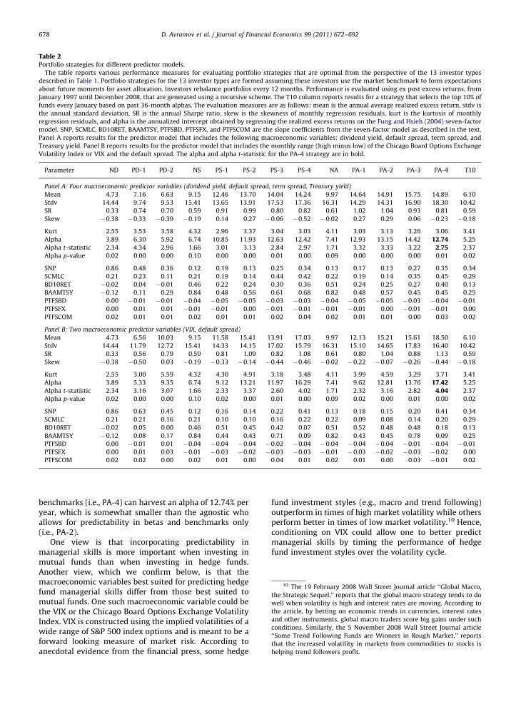
Table 2Portfolio strategies for different predictor models.

The table reports various performance measures for evaluating portfolio strategies that are optimal from the perspective of the 13 investor types

described in Table 1. Portfolio strategies for the 13 investor types are formed assuming these investors use the market benchmark to form expectations

about future moments for asset allocation. Investors rebalance portfolios every 12 months. Performance is evaluated using ex post excess returns, from

January 1997 until December 2008, that are generated using a recursive scheme. The T10 column reports results for a strategy that selects the top 10% of

funds every January based on past 36-month alphas. The evaluation measures are as follows: mean is the annual average realized excess return, stdv is

the annual standard deviation, SR is the annual Sharpe ratio, skew is the skewness of monthly regression residuals, kurt is the kurtosis of monthly

regression residuals, and alpha is the annualized intercept obtained by regressing the realized excess returns on the Fung and Hsieh (2004) seven-factor

model. SNP, SCMLC, BD10RET, BAAMTSY, PTFSBD, PTFSFX, and PTFSCOM are the slope coefficients from the seven-factor model as described in the text.

Panel A reports results for the predictor model that includes the following macroeconomic variables: dividend yield, default spread, term spread, and

Treasury yield. Panel B reports results for the predictor model that includes the monthly range (high minus low) of the Chicago Board Options Exchange

Volatility Index or VIX and the default spread. The alpha and alpha t-statistic for the PA-4 strategy are in bold.

Parameter ND PD-1 PD-2 NS PS-1 PS-2 PS-3 PS-4 NA PA-1 PA-2 PA-3 PA-4 T10

Panel A: Four macroeconomic predictor variables (dividend yield, default spread, term spread, Treasury yield)

Mean 4.73 7.16 6.63 9.15 12.46 13.70 14.04 14.24 9.97 14.64 14.91 15.75 14.89 6.10

Stdv 14.44 9.74 9.53 15.41 13.65 13.91 17.53 17.36 16.31 14.29 14.31 16.90 18.30 10.42

SR 0.33 0.74 0.70 0.59 0.91 0.99 0.80 0.82 0.61 1.02 1.04 0.93 0.81 0.59

Skew �0.38 �0.33 �0.39 �0.19 0.14 0.27 �0.06 �0.52 �0.02 0.27 0.29 0.06 �0.23 �0.18

Kurt 2.55 3.53 3.58 4.32 2.96 3.37 3.04 3.03 4.11 3.03 3.13 3.26 3.06 3.41

Alpha 3.89 6.30 5.92 6.74 10.85 11.93 12.63 12.42 7.41 12.93 13.15 14.42 12.74 5.25

Alpha t-statistic 2.34 4.34 2.96 1.66 3.01 3.13 2.84 2.97 1.71 3.32 3.33 3.22 2.75 2.37

Alpha p-value 0.02 0.00 0.00 0.10 0.00 0.00 0.01 0.00 0.09 0.00 0.00 0.00 0.01 0.02

SNP 0.86 0.48 0.36 0.12 0.19 0.13 0.25 0.34 0.13 0.17 0.13 0.27 0.35 0.34

SCMLC 0.21 0.23 0.11 0.21 0.19 0.14 0.44 0.42 0.22 0.19 0.14 0.35 0.45 0.29

BD10RET �0.02 0.04 �0.01 0.46 0.22 0.24 0.30 0.36 0.51 0.24 0.25 0.27 0.40 0.13

BAAMTSY �0.12 0.11 0.29 0.84 0.48 0.56 0.61 0.68 0.82 0.48 0.57 0.45 0.45 0.25

PTFSBD 0.00 �0.01 �0.01 �0.04 �0.05 �0.05 �0.03 �0.03 �0.04 �0.05 �0.05 �0.03 �0.04 �0.01

PTFSFX 0.00 0.01 0.01 �0.01 �0.01 0.00 �0.01 �0.01 �0.01 �0.01 0.00 �0.01 �0.01 0.00

PTFSCOM 0.02 0.01 0.01 0.02 0.01 0.01 0.02 0.04 0.02 0.01 0.01 0.00 0.03 0.02

Panel B: Two macroeconomic predictor variables (VIX, default spread)

Mean 4.73 6.56 10.03 9.15 11.58 15.41 13.91 17.03 9.97 12.13 15.21 15.61 18.50 6.10

Stdv 14.44 11.79 12.72 15.41 14.33 14.15 17.02 15.79 16.31 15.10 14.65 17.83 16.40 10.42

SR 0.33 0.56 0.79 0.59 0.81 1.09 0.82 1.08 0.61 0.80 1.04 0.88 1.13 0.59

Skew �0.38 �0.50 0.03 �0.19 �0.33 �0.14 �0.44 �0.46 �0.02 �0.22 �0.07 �0.26 �0.44 �0.18

Kurt 2.55 3.00 5.59 4.32 4.30 4.91 3.18 3.48 4.11 3.99 4.59 3.29 3.71 3.41

Alpha 3.89 5.33 9.35 6.74 9.12 13.21 11.97 16.29 7.41 9.62 12.81 13.76 17.42 5.25

Alpha t-statistic 2.34 3.16 3.07 1.66 2.33 3.37 2.60 4.02 1.71 2.32 3.16 2.82 4.04 2.37

Alpha p-value 0.02 0.00 0.00 0.10 0.02 0.00 0.01 0.00 0.09 0.02 0.00 0.01 0.00 0.02

SNP 0.86 0.63 0.45 0.12 0.16 0.14 0.22 0.41 0.13 0.18 0.15 0.20 0.41 0.34

SCMLC 0.21 0.21 0.16 0.21 0.10 0.10 0.16 0.22 0.22 0.09 0.08 0.14 0.20 0.29

BD10RET �0.02 0.05 0.00 0.46 0.51 0.45 0.42 0.07 0.51 0.52 0.48 0.48 0.18 0.13

BAAMTSY �0.12 0.08 0.17 0.84 0.44 0.43 0.71 0.09 0.82 0.43 0.45 0.78 0.09 0.25

PTFSBD 0.00 �0.01 0.01 �0.04 �0.04 �0.04 �0.02 �0.04 �0.04 �0.04 �0.04 �0.01 �0.04 �0.01

PTFSFX 0.00 0.01 0.03 �0.01 �0.03 �0.02 �0.03 �0.03 �0.01 �0.03 �0.02 �0.03 �0.02 0.00

PTFSCOM 0.02 0.02 0.00 0.02 0.01 0.00 0.04 0.01 0.02 0.01 0.00 0.03 �0.01 0.02

10 The 19 February 2008 Wall Street Journal article ‘‘Global Macro,

the Strategic Sequel,’’ reports that the global macro strategy tends to do

well when volatility is high and interest rates are moving. According to

the article, by betting on economic trends in currencies, interest rates

and other instruments, global macro traders score big gains under such

conditions. Similarly, the 5 November 2008 Wall Street Journal article

‘‘Some Trend Following Funds are Winners in Rough Market,’’ reports

that the increased volatility in markets from commodities to stocks is

helping trend followers profit.

D. Avramov et al. / Journal of Financial Economics 99 (2011) 672–692678

benchmarks (i.e., PA-4) can harvest an alpha of 12.74% peryear, which is somewhat smaller than the agnostic whoallows for predictability in betas and benchmarks only(i.e., PA-2).

One view is that incorporating predictability inmanagerial skills is more important when investing inmutual funds than when investing in hedge funds.Another view, which we confirm below, is that themacroeconomic variables best suited for predicting hedgefund managerial skills differ from those best suited tomutual funds. One such macroeconomic variable could bethe VIX or the Chicago Board Options Exchange VolatilityIndex. VIX is constructed using the implied volatilities of awide range of S&P 500 index options and is meant to be aforward looking measure of market risk. According toanecdotal evidence from the financial press, some hedge

fund investment styles (e.g., macro and trend following)outperform in times of high market volatility while othersperform better in times of low market volatility.10 Hence,conditioning on VIX could allow one to better predictmanagerial skills by timing the performance of hedgefund investment styles over the volatility cycle.

D. Avramov et al. / Journal of Financial Economics 99 (2011) 672–692 679

Moreover, in the presence of estimation errors, it couldbe judicious to work with a more parsimonious con-ditioning framework. For example, Jagannathan and Wang(1996), in their work on the conditional Capital AssetPricing Model (CAPM), raise the issue of severe estimationerrors in the presence of multiple predictors. To minimizeestimation errors, they run a horse race across predictorsand ultimately use the default spread. Avramov andChordia (2006a) also appeal to a single predictor, i.e.,the default spread. Sharp increases in the defaultspread are often indicative of flights to quality, whichhave been linked anecdotally to significant deteriorat-ions in the performance of various hedge fund strategies(Lowenstein, 2000).

Motivated by these concerns, we consider predictabil-ity based simply on the default spread and a measure ofVIX, i.e., the lagged one-month high minus low VIX(henceforth VIX range), and rerun the out-of-sampleanalysis. Similar inferences obtain when using contem-poraneous monthly VIX, lagged one-month VIX, orstandard deviation of VIX. The results are reported inPanel B of Table 2. The evidence indicates that hedge fundinvestors are rewarded for incorporating predictability inmanagerial skills, at least when the predictable variationin hedge fund returns is conditioned on our parsimoniousset of macroeconomic variables. The PA-4 agnostic whoallows for predictability in alpha, betas, and benchmarkscan achieve an impressive out-of-sample alpha of 17.42%per year. This is over 13% per year higher than the alpha ofthe investor who excludes predictability altogether (ND),over 7% per year higher than the alphas of investors whoallow for predictability in betas only (PD-1, PS-1, andPA-1), and over 4% per year higher than the alphas ofinvestors who allow for predictability in betas andbenchmarks only (PD-2, PS-2, and PA-2). It is interestingto compare our results with those of Kosowski, Naik, andTeo (2007), who evaluate the out-of-sample performanceof a similar set of hedge funds. We replicate theirmethodology and find that the PA-4 investor outperformsthe strategy that invests in the top 10% of funds based onpast risk-adjusted performance, regardless of whetherrisk-adjusted performance is measured using past 36-month OLS alpha (henceforth T10) or past two-yearBayesian posterior alpha (henceforth KNT). Relative toour PA-3 and PA-4 investors, the T10 and KNT investorsearn lower ex post Fung and Hsieh (2004) alphas of 5.25%and 4.37% per year, respectively.11

4.2. Results by investment style

One concern is that our results might not be robustacross investment styles. That is, the benefits to predictingmanagerial skills could be driven by predictability in theperformance of a certain investment style only. To checkthis, we redo the out-of-sample optimal portfolio analysisfor each of our major investment styles: equity long/short,

11 To facilitate meaningful comparison, for the construction of the

T10 and KNT portfolios, we use the same set of funds used to form our

optimal strategy portfolios.

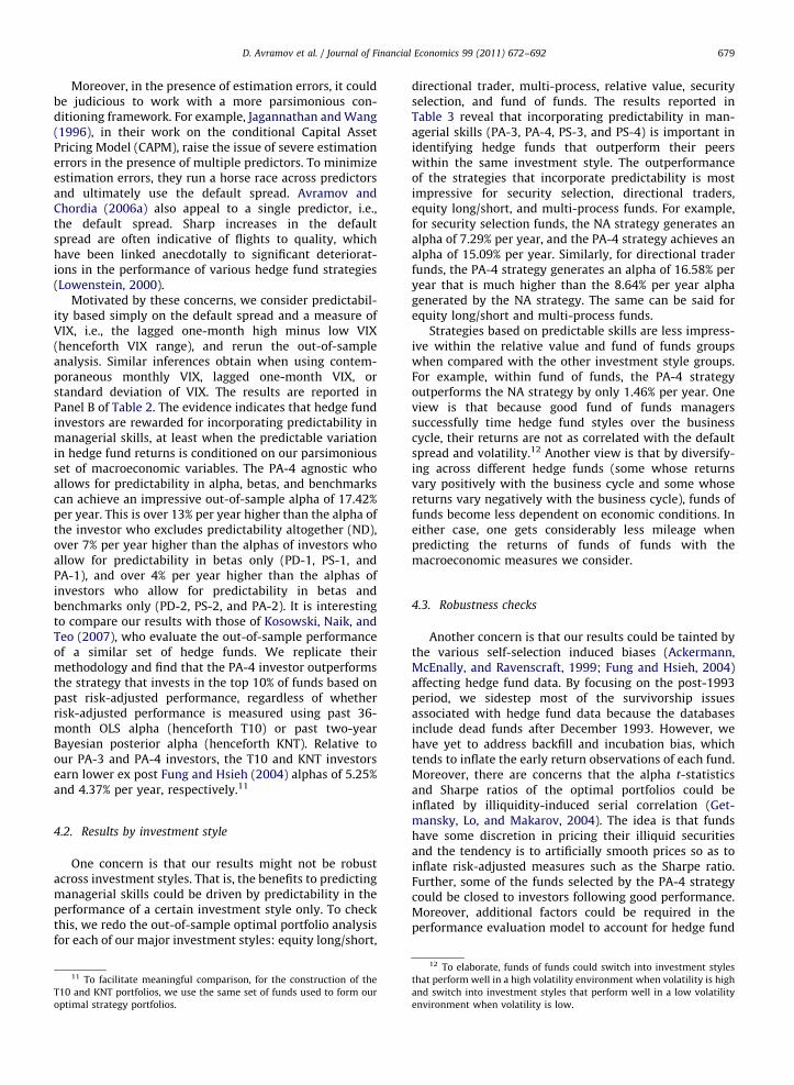
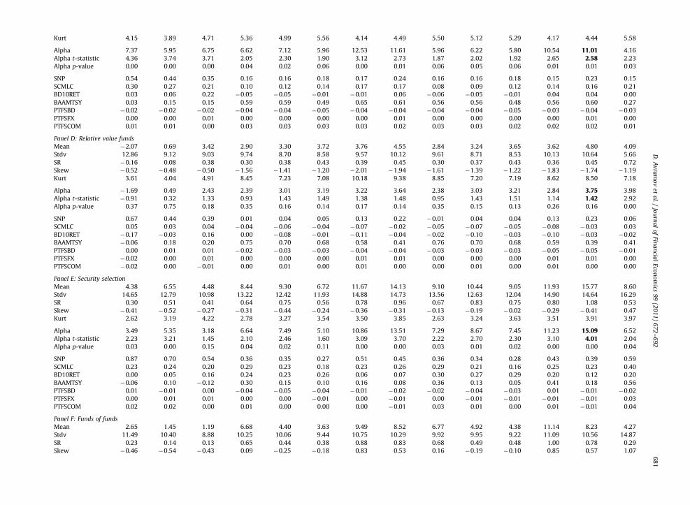
directional trader, multi-process, relative value, securityselection, and fund of funds. The results reported inTable 3 reveal that incorporating predictability in man-agerial skills (PA-3, PA-4, PS-3, and PS-4) is important inidentifying hedge funds that outperform their peerswithin the same investment style. The outperformanceof the strategies that incorporate predictability is mostimpressive for security selection, directional traders,equity long/short, and multi-process funds. For example,for security selection funds, the NA strategy generates analpha of 7.29% per year, and the PA-4 strategy achieves analpha of 15.09% per year. Similarly, for directional traderfunds, the PA-4 strategy generates an alpha of 16.58% peryear that is much higher than the 8.64% per year alphagenerated by the NA strategy. The same can be said forequity long/short and multi-process funds.

Strategies based on predictable skills are less impress-ive within the relative value and fund of funds groupswhen compared with the other investment style groups.For example, within fund of funds, the PA-4 strategyoutperforms the NA strategy by only 1.46% per year. Oneview is that because good fund of funds managerssuccessfully time hedge fund styles over the businesscycle, their returns are not as correlated with the defaultspread and volatility.12 Another view is that by diversify-ing across different hedge funds (some whose returnsvary positively with the business cycle and some whosereturns vary negatively with the business cycle), funds offunds become less dependent on economic conditions. Ineither case, one gets considerably less mileage whenpredicting the returns of funds of funds with themacroeconomic measures we consider.

4.3. Robustness checks

Another concern is that our results could be tainted bythe various self-selection induced biases (Ackermann,McEnally, and Ravenscraft, 1999; Fung and Hsieh, 2004)affecting hedge fund data. By focusing on the post-1993period, we sidestep most of the survivorship issuesassociated with hedge fund data because the databasesinclude dead funds after December 1993. However, wehave yet to address backfill and incubation bias, whichtends to inflate the early return observations of each fund.Moreover, there are concerns that the alpha t-statisticsand Sharpe ratios of the optimal portfolios could beinflated by illiquidity-induced serial correlation (Get-mansky, Lo, and Makarov, 2004). The idea is that fundshave some discretion in pricing their illiquid securitiesand the tendency is to artificially smooth prices so as toinflate risk-adjusted measures such as the Sharpe ratio.Further, some of the funds selected by the PA-4 strategycould be closed to investors following good performance.Moreover, additional factors could be required in theperformance evaluation model to account for hedge fund

12 To elaborate, funds of funds could switch into investment styles

that perform well in a high volatility environment when volatility is high

and switch into investment styles that perform well in a low volatility

environment when volatility is low.

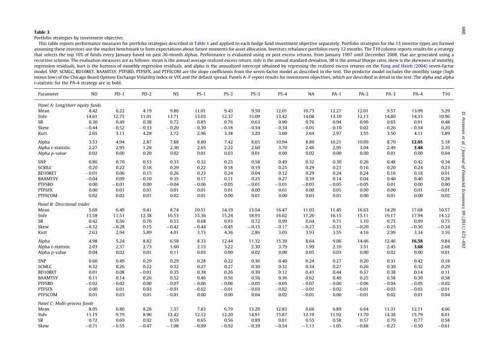
Table 3Portfolio strategies by investment objective.

This table reports performance measures for portfolio strategies described in Table 1 and applied to each hedge fund investment objective separately. Portfolio strategies for the 13 investor types are formed

assuming these investors use the market benchmark to form expectations about future moments for asset allocation. Investors rebalance portfolios every 12 months. The T10 column reports results for a strategy

that selects the top 10% of funds every January based on past 36-month alphas. Performance is evaluated using ex post excess returns, from January 1997 until December 2008, that are generated using a

recursive scheme. The evaluation measures are as follows: mean is the annual average realized excess return, stdv is the annual standard deviation, SR is the annual Sharpe ratio, skew is the skewness of monthly

regression residuals, kurt is the kurtosis of monthly regression residuals, and alpha is the annualized intercept obtained by regressing the realized excess returns on the Fung and Hsieh (2004) seven-factor

model. SNP, SCMLC, BD10RET, BAAMTSY, PTFSBD, PTFSFX, and PTFSCOM are the slope coefficients from the seven-factor model as described in the text. The predictor model includes the monthly range (high

minus low) of the Chicago Board Options Exchange Volatility Index or VIX and the default spread. Panels A–F report results for investment objectives, which are described in detail in the text. The alpha and alpha

t-statistic for the PA-4 strategy are in bold.

Parameter ND PD-1 PD-2 NS PS-1 PS-2 PS-3 PS-4 NA PA-1 PA-2 PA-3 PA-4 T10

Panel A: Long/short equity funds

Mean 4.42 6.22 4.19 9.86 11.01 9.43 9.50 12.01 10.73 12.27 12.01 9.57 13.09 5.29

Stdv 14.61 12.75 11.01 13.71 13.03 12.37 15.09 13.42 14.08 13.10 12.13 14.80 14.33 10.96

SR 0.30 0.49 0.38 0.72 0.85 0.76 0.63 0.90 0.76 0.94 0.99 0.65 0.91 0.48

Skew �0.44 �0.52 �0.33 �0.20 �0.30 �0.18 �0.34 �0.34 �0.01 �0.10 0.02 �0.26 �0.34 0.20

Kurt 2.65 3.11 4.28 2.72 2.96 3.38 3.20 3.60 2.64 2.97 3.55 3.50 4.11 3.89

Alpha 3.53 4.94 2.87 7.88 8.80 7.42 8.65 10.94 8.80 10.21 10.09 8.70 12.05 5.18

Alpha t-statistic 2.27 2.95 1.28 2.30 2.65 2.22 2.60 3.70 2.46 2.95 3.04 2.49 3.48 2.10

Alpha p-value 0.02 0.00 0.20 0.02 0.01 0.03 0.01 0.00 0.02 0.00 0.00 0.01 0.00 0.04

SNP 0.86 0.70 0.53 0.33 0.32 0.25 0.58 0.49 0.32 0.30 0.26 0.48 0.42 0.34

SCMLC 0.20 0.22 0.18 0.29 0.22 0.18 0.19 0.25 0.29 0.21 0.16 0.20 0.24 0.23

BD10RET �0.01 0.06 0.15 0.26 0.23 0.24 0.04 0.12 0.29 0.24 0.24 0.16 0.18 0.01

BAAMTSY �0.04 0.09 �0.10 0.35 0.17 0.11 0.25 0.27 0.39 0.14 0.04 0.40 0.40 0.28

PTFSBD 0.00 �0.01 0.00 �0.04 �0.06 �0.05 �0.01 �0.01 �0.03 �0.05 �0.05 0.01 0.00 0.00

PTFSFX 0.00 0.01 0.01 0.01 0.01 0.01 0.00 0.01 0.00 0.01 0.00 0.00 0.01 �0.01

PTFSCOM 0.02 0.02 0.01 0.02 0.01 0.00 0.01 0.00 0.03 0.01 0.00 0.01 0.00 0.02

Panel B: Directional trader

Mean 5.69 6.49 9.41 8.74 10.51 14.19 13.54 16.47 11.03 11.45 16.63 14.29 17.68 10.57

Stdv 13.58 11.51 12.38 16.53 15.36 15.24 18.93 16.62 17.20 16.15 15.11 19.17 17.94 14.12

SR 0.42 0.56 0.76 0.53 0.68 0.93 0.72 0.99 0.64 0.71 1.10 0.75 0.99 0.75

Skew �0.32 �0.28 0.15 �0.42 �0.44 �0.45 �0.15 �0.17 �0.27 �0.33 �0.20 �0.25 �0.36 �0.34

Kurt 2.63 2.94 5.89 4.01 3.73 4.36 2.86 3.03 3.93 3.55 4.16 2.99 3.34 3.16

Alpha 4.98 5.24 8.82 6.58 8.33 12.44 11.32 15.39 8.64 9.06 14.46 12.46 16.58 9.84

Alpha t-statistic 2.03 2.37 2.73 1.60 2.15 3.22 2.30 3.79 1.99 2.19 3.51 2.45 3.68 2.68

Alpha p-value 0.04 0.02 0.01 0.11 0.03 0.00 0.02 0.00 0.05 0.03 0.00 0.02 0.00 0.01

SNP 0.60 0.49 0.29 0.29 0.28 0.22 0.36 0.40 0.24 0.27 0.20 0.31 0.42 0.18

SCMLC 0.32 0.26 0.22 0.32 0.27 0.27 0.30 0.32 0.34 0.27 0.26 0.30 0.32 0.29

BD10RET 0.01 0.08 �0.01 0.35 0.38 0.26 0.39 0.12 0.41 0.44 0.37 0.38 0.14 0.11

BAAMTSY 0.11 0.14 0.26 0.52 0.46 0.56 0.56 0.36 0.62 0.49 0.25 0.58 0.30 0.58

PTFSBD �0.02 �0.02 0.00 �0.07 �0.06 �0.06 �0.05 �0.05 �0.07 �0.06 �0.06 �0.04 �0.05 �0.02

PTFSFX 0.00 0.01 0.03 �0.01 �0.02 �0.01 �0.03 �0.02 �0.01 �0.02 �0.01 �0.03 �0.03 �0.01

PTFSCOM 0.01 0.03 0.01 �0.01 0.00 0.00 0.04 0.02 �0.01 0.00 �0.01 0.02 0.01 0.04

Panel C: Multi-process funds

Mean 8.05 6.80 8.26 7.37 7.83 6.79 13.29 12.83 6.66 6.89 6.64 11.31 12.11 4.66

Stdv 11.15 9.79 8.96 12.42 12.12 12.20 14.91 15.87 12.19 11.92 11.70 14.38 15.79 8.01

SR 0.72 0.69 0.92 0.59 0.65 0.56 0.89 0.81 0.55 0.58 0.57 0.79 0.77 0.58

Skew �0.71 �0.55 �0.47 �1.08 �0.99 �0.92 �0.39 �0.54 �1.11 �1.05 �0.88 �0.27 �0.50 �0.61

D.

Av

ram

ov

eta

l./

Jou

rna

lo

fFin

an

cial

Eco

no

mics

99

(20

11

)6

72

–6

92

68

0

Kurt 4.15 3.89 4.71 5.36 4.99 5.56 4.14 4.49 5.50 5.12 5.29 4.17 4.44 5.58

Alpha 7.37 5.95 6.75 6.62 7.12 5.96 12.53 11.61 5.96 6.22 5.80 10.54 11.01 4.16

Alpha t-statistic 4.36 3.74 3.71 2.05 2.30 1.90 3.12 2.73 1.87 2.02 1.92 2.65 2.58 2.23

Alpha p-value 0.00 0.00 0.00 0.04 0.02 0.06 0.00 0.01 0.06 0.05 0.06 0.01 0.01 0.03

SNP 0.54 0.44 0.35 0.16 0.16 0.18 0.17 0.24 0.16 0.16 0.18 0.15 0.23 0.15

SCMLC 0.30 0.27 0.21 0.10 0.12 0.14 0.17 0.17 0.08 0.09 0.12 0.14 0.16 0.21

BD10RET 0.03 0.06 0.22 �0.05 �0.05 �0.01 �0.01 0.06 �0.06 �0.05 �0.01 0.04 0.04 0.00

BAAMTSY 0.03 0.15 0.15 0.59 0.59 0.49 0.65 0.61 0.56 0.56 0.48 0.56 0.60 0.27

PTFSBD �0.02 �0.02 �0.02 �0.04 �0.04 �0.05 �0.04 �0.04 �0.04 �0.04 �0.05 �0.03 �0.04 �0.03

PTFSFX 0.00 0.00 0.01 0.00 0.00 0.00 0.00 0.01 0.00 0.00 0.00 0.00 0.01 0.00

PTFSCOM 0.01 0.01 0.00 0.03 0.03 0.03 0.03 0.02 0.03 0.03 0.02 0.02 0.02 0.01

Panel D: Relative value funds

Mean �2.07 0.69 3.42 2.90 3.30 3.72 3.76 4.55 2.84 3.24 3.65 3.62 4.80 4.09

Stdv 12.86 9.12 9.03 9.74 8.70 8.58 9.57 10.12 9.61 8.71 8.53 10.13 10.64 5.66

SR �0.16 0.08 0.38 0.30 0.38 0.43 0.39 0.45 0.30 0.37 0.43 0.36 0.45 0.72

Skew �0.52 �0.48 �0.50 �1.56 �1.41 �1.20 �2.01 �1.94 �1.61 �1.39 �1.22 �1.83 �1.74 �1.19

Kurt 3.61 4.04 4.91 8.45 7.23 7.08 10.18 9.38 8.85 7.20 7.19 8.62 8.50 7.18

Alpha �1.69 0.49 2.43 2.39 3.01 3.19 3.22 3.64 2.38 3.03 3.21 2.84 3.75 3.98

Alpha t-statistic �0.91 0.32 1.33 0.93 1.43 1.49 1.38 1.48 0.95 1.43 1.51 1.14 1.42 2.92

Alpha p-value 0.37 0.75 0.18 0.35 0.16 0.14 0.17 0.14 0.35 0.15 0.13 0.26 0.16 0.00

SNP 0.67 0.44 0.39 0.01 0.04 0.05 0.13 0.22 �0.01 0.04 0.04 0.13 0.23 0.06

SCMLC 0.05 0.03 0.04 �0.04 �0.06 �0.04 �0.07 �0.02 �0.05 �0.07 �0.05 �0.08 �0.03 0.03

BD10RET �0.17 �0.03 0.16 0.00 �0.08 �0.01 �0.11 �0.04 �0.02 �0.10 �0.03 �0.10 �0.03 �0.02

BAAMTSY �0.06 0.18 0.20 0.75 0.70 0.68 0.58 0.41 0.76 0.70 0.68 0.59 0.39 0.41

PTFSBD 0.00 0.01 0.01 �0.02 �0.03 �0.03 �0.04 �0.04 �0.03 �0.03 �0.03 �0.05 �0.05 �0.01

PTFSFX �0.02 0.00 0.01 0.00 0.00 0.00 0.01 0.01 0.00 0.00 0.00 0.01 0.01 0.00

PTFSCOM �0.02 0.00 �0.01 0.00 0.01 0.00 0.01 0.00 0.00 0.01 0.00 0.01 0.00 0.00

Panel E: Security selection

Mean 4.38 6.55 4.48 8.44 9.30 6.72 11.67 14.13 9.10 10.44 9.05 11.93 15.77 8.60

Stdv 14.65 12.79 10.98 13.22 12.42 11.93 14.88 14.73 13.56 12.63 12.04 14.90 14.64 16.29

SR 0.30 0.51 0.41 0.64 0.75 0.56 0.78 0.96 0.67 0.83 0.75 0.80 1.08 0.53

Skew �0.41 �0.52 �0.27 �0.31 �0.44 �0.24 �0.36 �0.31 �0.13 �0.19 �0.02 �0.29 �0.41 0.47

Kurt 2.62 3.19 4.22 2.78 3.27 3.54 3.50 3.85 2.63 3.24 3.63 3.51 3.91 3.97

Alpha 3.49 5.35 3.18 6.64 7.49 5.10 10.86 13.51 7.29 8.67 7.45 11.23 15.09 6.52

Alpha t-statistic 2.23 3.21 1.45 2.10 2.46 1.60 3.09 3.70 2.22 2.70 2.30 3.10 4.01 2.04

Alpha p-value 0.03 0.00 0.15 0.04 0.02 0.11 0.00 0.00 0.03 0.01 0.02 0.00 0.00 0.04

SNP 0.87 0.70 0.54 0.36 0.35 0.27 0.51 0.45 0.36 0.34 0.28 0.43 0.39 0.59

SCMLC 0.23 0.24 0.20 0.29 0.23 0.18 0.23 0.26 0.29 0.21 0.16 0.25 0.23 0.40

BD10RET 0.00 0.05 0.16 0.24 0.23 0.26 0.06 0.07 0.30 0.27 0.29 0.20 0.12 0.20

BAAMTSY �0.06 0.10 �0.12 0.30 0.15 0.10 0.16 0.08 0.36 0.13 0.05 0.41 0.18 0.56

PTFSBD 0.01 �0.01 0.00 �0.04 �0.05 �0.04 �0.01 �0.02 �0.02 �0.04 �0.03 0.01 �0.01 �0.02

PTFSFX 0.00 0.01 0.01 0.00 0.00 �0.01 0.00 �0.01 0.00 �0.01 �0.01 �0.01 �0.01 0.03

PTFSCOM 0.02 0.02 0.00 0.01 0.00 0.00 0.00 �0.01 0.03 0.01 0.00 0.01 �0.01 0.04

Panel F: Funds of funds

Mean 2.65 1.45 1.19 6.68 4.40 3.63 9.49 8.52 6.77 4.92 4.38 11.14 8.23 4.27

Stdv 11.49 10.40 8.88 10.25 10.06 9.44 10.75 10.29 9.92 9.95 9.22 11.09 10.56 14.87

SR 0.23 0.14 0.13 0.65 0.44 0.38 0.88 0.83 0.68 0.49 0.48 1.00 0.78 0.29

Skew �0.46 �0.54 �0.43 0.09 �0.25 �0.18 0.83 0.53 0.16 �0.19 �0.10 0.85 0.57 1.07

D.

Av

ram

ov

eta

l./

Jou

rna

lo

fFin

an

cial

Eco

no

mics

99

(20

11

)6

72

–6

92

68

1

Ta

ble

3(c

on

tin

ued

)

Pa

ram

ete

rN

DP

D-1

PD

-2N

SP

S-1

PS

-2P

S-3

PS

-4N

AP

A-1

PA

-2P

A-3

PA

-4T

10

Ku

rt3

.72

3.9

14

.02

3.9

44

.01

4.2

04

.74

5.4

73

.82

4.0

64

.14

4.4

76

.35

7.0

4

Alp

ha

1.6

40

.53

�0

.03

5.9

73

.43

2.5

89

.64

7.8

76

.07

3.9

93

.39

10

.60

7.5

33

.15

Alp

ha

t-st

ati

stic

0.7

70

.25

�0

.02

2.1

81

.29

1.0

43

.24

2.9

42

.25

1.4

91

.37

3.4

42

.76

0.7

6

Alp

ha

p-v

alu

e0

.44

0.8

00

.99

0.0

30

.20

0.3

00

.00

0.0

00

.03

0.1

40

.17

0.0

00

.01

0.4

5

SN

P0

.45

0.3

40

.22

0.1

90

.17

0.1

40

.15

0.2

20

.17

0.1

50

.13

0.1

90

.23

0.3

1

SC

MLC

0.2

50

.21

0.1

70

.16

0.1

90

.18

0.2

90

.31

0.1

50

.18

0.1

70

.28

0.3

30

.09

BD

10

RE

T0

.04

0.0

60

.18

0.1

00

.13

0.1

3�

0.0

60

.03

0.1

00

.14

0.1

30

.06

0.0

30

.29

BA

AM

TS

Y0

.35

0.4

30

.38

0.3

40

.36

0.3

5�

0.1

8�

0.3

30

.31

0.3

20

.30

�0

.17

�0

.33

0.1

6

PT

FSB

D�

0.0

2�

0.0

1�

0.0

10

.00

�0

.01

�0

.02

�0

.01

�0

.04

0.0

0�

0.0

1�

0.0

2�

0.0

1�

0.0

40

.05

PT

FSFX

0.0

10

.01

0.0

00

.01

0.0

10

.00

0.0

00

.00

0.0

10

.01

0.0

00

.00

0.0

00

.00

PT

FSC

OM

0.0

20

.03

0.0

20

.02

0.0

20

.03

0.0

20

.02

0.0

10

.02

0.0

20

.02

0.0

20

.05

D. Avramov et al. / Journal of Financial Economics 99 (2011) 672–692682

exposure to emerging markets, distress risk (Fama andFrench, 1993), stock momentum (Jegadeesh and Titman,1993), and illiquidity (Pastor and Stambaugh, 2003).

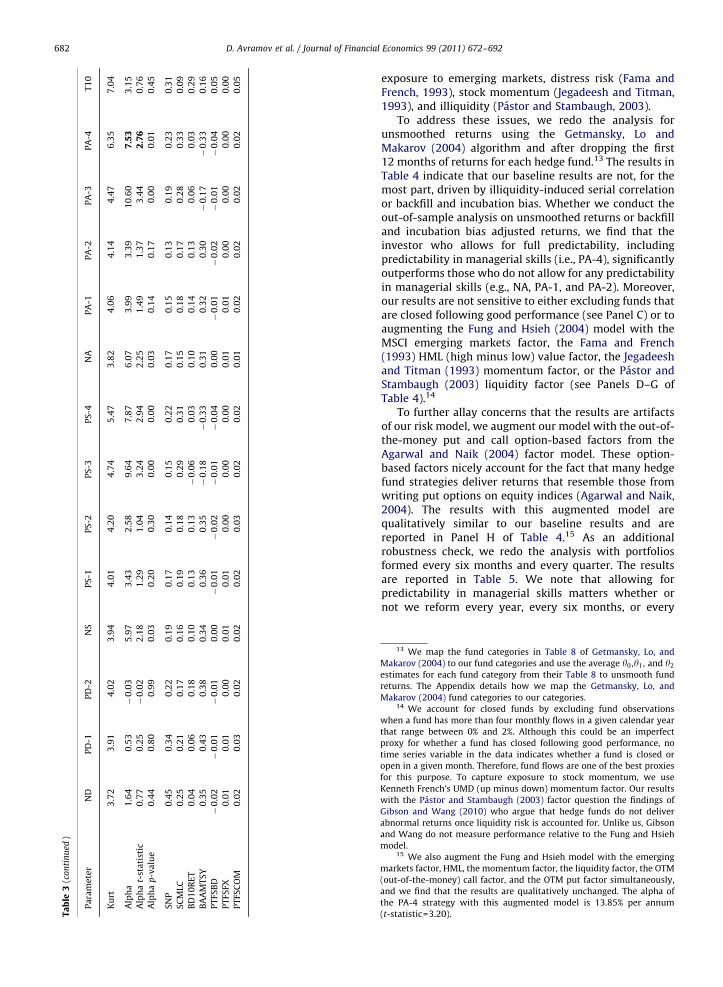
To address these issues, we redo the analysis forunsmoothed returns using the Getmansky, Lo andMakarov (2004) algorithm and after dropping the first12 months of returns for each hedge fund.13 The results inTable 4 indicate that our baseline results are not, for themost part, driven by illiquidity-induced serial correlationor backfill and incubation bias. Whether we conduct theout-of-sample analysis on unsmoothed returns or backfilland incubation bias adjusted returns, we find that theinvestor who allows for full predictability, includingpredictability in managerial skills (i.e., PA-4), significantlyoutperforms those who do not allow for any predictabilityin managerial skills (e.g., NA, PA-1, and PA-2). Moreover,our results are not sensitive to either excluding funds thatare closed following good performance (see Panel C) or toaugmenting the Fung and Hsieh (2004) model with theMSCI emerging markets factor, the Fama and French(1993) HML (high minus low) value factor, the Jegadeeshand Titman (1993) momentum factor, or the Pastor andStambaugh (2003) liquidity factor (see Panels D–G ofTable 4).14

To further allay concerns that the results are artifactsof our risk model, we augment our model with the out-of-the-money put and call option-based factors from theAgarwal and Naik (2004) factor model. These option-based factors nicely account for the fact that many hedgefund strategies deliver returns that resemble those fromwriting put options on equity indices (Agarwal and Naik,2004). The results with this augmented model arequalitatively similar to our baseline results and arereported in Panel H of Table 4.15 As an additionalrobustness check, we redo the analysis with portfoliosformed every six months and every quarter. The resultsare reported in Table 5. We note that allowing forpredictability in managerial skills matters whether ornot we reform every year, every six months, or every

13 We map the fund categories in Table 8 of Getmansky, Lo, and

Makarov (2004) to our fund categories and use the average y0 ,y1 , and y2

estimates for each fund category from their Table 8 to unsmooth fund

returns. The Appendix details how we map the Getmansky, Lo, and

Makarov (2004) fund categories to our categories.14 We account for closed funds by excluding fund observations

when a fund has more than four monthly flows in a given calendar year

that range between 0% and 2%. Although this could be an imperfect

proxy for whether a fund has closed following good performance, no

time series variable in the data indicates whether a fund is closed or

open in a given month. Therefore, fund flows are one of the best proxies

for this purpose. To capture exposure to stock momentum, we use

Kenneth French’s UMD (up minus down) momentum factor. Our results

with the Pastor and Stambaugh (2003) factor question the findings of

Gibson and Wang (2010) who argue that hedge funds do not deliver

abnormal returns once liquidity risk is accounted for. Unlike us, Gibson

and Wang do not measure performance relative to the Fung and Hsieh

model.15 We also augment the Fung and Hsieh model with the emerging

markets factor, HML, the momentum factor, the liquidity factor, the OTM

(out-of-the-money) call factor, and the OTM put factor simultaneously,

and we find that the results are qualitatively unchanged. The alpha of

the PA-4 strategy with this augmented model is 13.85% per annum

(t-statistic=3.20).

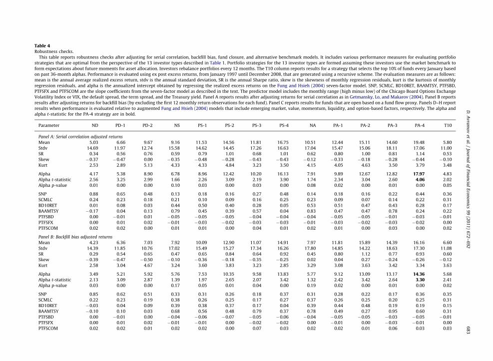
Table 4Robustness checks.

This table reports robustness checks after adjusting for serial correlation, backfill bias, fund closure, and alternative benchmark models. It includes various performance measures for evaluating portfolio

strategies that are optimal from the perspective of the 13 investor types described in Table 1. Portfolio strategies for the 13 investor types are formed assuming these investors use the market benchmark to

form expectations about future moments for asset allocation. Investors rebalance portfolios every 12 months. The T10 column reports results for a strategy that selects the top 10% of funds every January based

on past 36-month alphas. Performance is evaluated using ex post excess returns, from January 1997 until December 2008, that are generated using a recursive scheme. The evaluation measures are as follows:

mean is the annual average realized excess return, stdv is the annual standard deviation, SR is the annual Sharpe ratio, skew is the skewness of monthly regression residuals, kurt is the kurtosis of monthly

regression residuals, and alpha is the annualized intercept obtained by regressing the realized excess returns on the Fung and Hsieh (2004) seven-factor model. SNP, SCMLC, BD10RET, BAAMTSY, PTFSBD,

PTFSFX and PTFSCOM are the slope coefficients from the seven-factor model as described in the text. The predictor model includes the monthly range (high minus low) of the Chicago Board Options Exchange

Volatility Index or VIX, the default spread, the term spread, and the Treasury yield. Panel A reports results after adjusting returns for serial correlation as in Getmansky, Lo, and Makarov (2004). Panel B reports

results after adjusting returns for backfill bias (by excluding the first 12 monthly return observations for each fund). Panel C reports results for funds that are open based on a fund flow proxy. Panels D–H report

results when performance is evaluated relative to augmented Fung and Hsieh (2004) models that include emerging market, value, momentum, liquidity, and option-based factors, respectively. The alpha and

alpha t-statistic for the PA-4 strategy are in bold.

Parameter ND PD-1 PD-2 NS PS-1 PS-2 PS-3 PS-4 NA PA-1 PA-2 PA-3 PA-4 T10

Panel A: Serial correlation adjusted returns

Mean 5.03 6.66 9.67 9.16 11.53 14.56 11.81 16.75 10.51 12.44 15.11 14.60 19.48 5.80

Stdv 14.69 11.97 12.74 15.58 14.62 14.45 17.26 16.63 17.04 15.47 15.06 18.11 17.06 11.00

SR 0.34 0.56 0.76 0.59 0.79 1.01 0.68 1.01 0.62 0.80 1.00 0.81 1.14 0.53

Skew �0.37 �0.47 0.00 �0.35 �0.48 �0.28 �0.43 �0.43 �0.12 �0.33 �0.18 �0.28 �0.44 �0.10

Kurt 2.53 2.89 5.13 4.33 4.33 4.84 3.23 3.50 4.15 4.05 4.63 3.50 3.79 3.48

Alpha 4.17 5.38 8.90 6.78 8.96 12.42 10.20 16.13 7.91 9.89 12.67 12.82 17.97 4.83

Alpha t-statistic 2.56 3.25 2.99 1.66 2.26 3.09 2.19 3.90 1.74 2.34 3.04 2.60 4.06 2.02

Alpha p-value 0.01 0.00 0.00 0.10 0.03 0.00 0.03 0.00 0.08 0.02 0.00 0.01 0.00 0.05

SNP 0.88 0.65 0.48 0.13 0.18 0.16 0.27 0.48 0.14 0.18 0.16 0.22 0.44 0.36

SCMLC 0.24 0.23 0.18 0.21 0.10 0.09 0.16 0.25 0.23 0.09 0.07 0.14 0.22 0.31

BD10RET 0.01 0.08 0.03 0.44 0.50 0.40 0.28 0.05 0.53 0.51 0.47 0.43 0.28 0.17

BAAMTSY �0.17 0.04 0.13 0.79 0.45 0.39 0.57 0.04 0.83 0.47 0.47 0.78 0.24 0.22

PTFSBD 0.00 �0.01 0.01 �0.05 �0.05 �0.05 �0.04 �0.04 �0.04 �0.05 �0.05 �0.01 �0.03 �0.01

PTFSFX 0.00 0.01 0.02 �0.01 �0.03 �0.02 �0.03 �0.03 �0.01 �0.03 �0.02 �0.03 �0.02 0.00

PTFSCOM 0.02 0.02 0.00 0.01 0.01 0.00 0.04 0.01 0.02 0.01 0.00 0.03 0.00 0.02

Panel B: Backfill bias adjusted returns

Mean 4.23 6.36 7.03 7.92 10.09 12.90 11.07 14.91 7.97 11.81 15.89 14.39 16.16 6.60

Stdv 14.39 11.85 10.76 17.02 15.49 15.27 17.34 16.26 17.80 14.85 14.22 18.63 17.30 11.08

SR 0.29 0.54 0.65 0.47 0.65 0.84 0.64 0.92 0.45 0.80 1.12 0.77 0.93 0.60

Skew �0.39 �0.47 �0.50 �0.10 �0.36 �0.18 �0.35 �0.25 0.02 0.04 0.27 �0.24 �0.26 �0.12

Kurt 2.58 3.04 4.67 3.24 3.60 3.83 3.23 2.85 3.29 3.08 3.63 3.42 3.34 3.63

Alpha 3.49 5.21 5.92 5.76 7.53 10.35 9.58 13.83 5.77 9.12 13.09 13.17 14.36 5.68

Alpha t-statistic 2.13 3.09 2.87 1.39 1.97 2.65 2.07 3.42 1.32 2.42 3.42 2.64 3.30 2.41

Alpha p-value 0.03 0.00 0.00 0.17 0.05 0.01 0.04 0.00 0.19 0.02 0.00 0.01 0.00 0.02

SNP 0.85 0.62 0.51 0.33 0.31 0.26 0.18 0.37 0.31 0.28 0.22 0.17 0.36 0.35

SCMLC 0.22 0.23 0.19 0.38 0.26 0.25 0.17 0.27 0.37 0.26 0.25 0.20 0.25 0.31

BD10RET �0.03 0.04 0.09 0.39 0.38 0.37 0.17 0.04 0.39 0.44 0.48 0.19 0.19 0.15

BAAMTSY �0.10 0.10 0.03 0.68 0.56 0.48 0.79 0.37 0.78 0.49 0.27 0.95 0.60 0.31

PTFSBD 0.00 �0.01 0.00 �0.04 �0.06 �0.07 �0.05 �0.06 �0.04 �0.05 �0.05 �0.03 �0.05 �0.01

PTFSFX 0.00 0.01 0.02 �0.01 �0.01 0.00 �0.02 �0.02 0.00 �0.01 0.00 �0.03 �0.01 0.00

PTFSCOM 0.02 0.02 0.01 0.02 0.02 0.00 0.07 0.03 0.02 0.02 0.01 0.06 0.03 0.03

D.

Av

ram

ov

eta

l./

Jou

rna

lo

fFin

an

cial

Eco

no

mics

99

(20

11

)6

72

–6

92

68

3

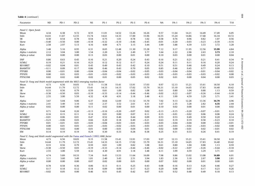
Table 4 (continued )

Parameter ND PD-1 PD-2 NS PS-1 PS-2 PS-3 PS-4 NA PA-1 PA-2 PA-3 PA-4 T10

Panel C: Open funds

Mean 4.34 6.38 9.72 8.55 11.01 14.52 13.26 16.26 9.57 11.64 14.21 14.49 17.49 6.05

Stdv 14.43 11.87 12.55 15.74 14.61 14.33 17.00 15.96 16.55 15.24 14.86 17.68 16.34 10.72

SR 0.30 0.54 0.78 0.54 0.75 1.01 0.78 1.02 0.58 0.76 0.96 0.82 1.07 0.56

Skew �0.40 �0.50 0.00 �0.18 �0.32 �0.10 �0.46 �0.45 -0.01 �0.20 �0.03 �0.23 �0.39 �0.16

Kurt 2.58 2.97 5.13 4.16 4.09 4.71 3.15 3.44 3.99 3.88 4.39 3.33 3.72 3.28

Alpha 3.48 5.16 8.95 6.31 8.65 12.48 11.30 15.28 7.12 9.17 11.95 12.56 15.99 4.84

Alpha t-statistic 2.12 3.04 3.00 1.54 2.20 3.21 2.49 3.77 1.64 2.22 2.96 2.63 3.73 2.10

Alpha p-value 0.04 0.00 0.00 0.13 0.03 0.00 0.01 0.00 0.10 0.03 0.00 0.01 0.00 0.04

SNP 0.86 0.63 0.45 0.16 0.21 0.20 0.24 0.43 0.16 0.21 0.21 0.21 0.41 0.34

SCMLC 0.19 0.21 0.16 0.23 0.12 0.12 0.17 0.24 0.24 0.11 0.11 0.16 0.20 0.24

BD10RET �0.02 0.04 0.01 0.45 0.49 0.43 0.42 0.10 0.51 0.51 0.46 0.49 0.24 0.13

BAAMTSY �0.11 0.09 0.17 0.86 0.46 0.43 0.70 0.05 0.85 0.46 0.45 0.77 0.09 0.33

PTFSBD 0.00 �0.01 0.00 �0.04 �0.04 �0.04 �0.02 �0.05 �0.03 �0.04 �0.04 �0.01 �0.04 �0.02

PTFSFX 0.00 0.01 0.03 �0.01 �0.03 �0.02 �0.03 �0.03 �0.01 �0.03 �0.03 �0.03 �0.02 0.00

PTFSCOM 0.02 0.02 0.00 0.02 0.01 0.00 0.05 0.02 0.02 0.01 0.00 0.04 0.00 0.03

Panel D: Fung and Hsieh model augmented with the MSCI emerging markets factor

Mean 4.73 6.56 10.03 9.15 11.58 15.41 13.91 17.03 9.97 12.13 15.21 15.61 18.50 6.10

Stdv 14.44 11.79 12.72 15.41 14.33 14.15 17.02 15.79 16.31 15.10 14.65 17.83 16.40 10.42

SR 0.33 0.56 0.79 0.59 0.81 1.09 0.82 1.08 0.61 0.80 1.04 0.88 1.13 0.59

Skew �0.38 �0.50 0.03 �0.19 �0.33 �0.14 �0.44 �0.46 �0.02 �0.22 �0.07 �0.26 �0.44 �0.18

Kurt 2.55 3.00 5.59 4.32 4.30 4.91 3.18 3.48 4.11 3.99 4.59 3.29 3.71 3.41

Alpha 3.67 5.04 9.06 6.37 8.64 12.69 11.52 15.70 7.02 9.13 12.28 13.36 16.79 4.96

Alpha t-statistic 2.41 3.49 3.10 1.63 2.37 3.52 2.61 4.31 1.67 2.35 3.28 2.82 4.35 2.44

Alpha p-value 0.02 0.00 0.00 0.11 0.02 0.00 0.01 0.00 0.10 0.02 0.00 0.01 0.00 0.02

SNP 0.71 0.44 0.26 �0.13 �0.16 �0.20 �0.07 0.02 �0.13 �0.15 �0.20 �0.07 �0.01 0.15

SCMLC 0.16 0.15 0.11 0.14 0.01 0.00 0.07 0.11 0.15 �0.01 �0.02 0.06 0.08 0.24

BD10RET �0.01 0.06 0.01 0.47 0.52 0.46 0.44 0.09 0.53 0.53 0.49 0.50 0.20 0.14

BAAMTSY �0.23 �0.06 0.03 0.66 0.20 0.18 0.49 �0.21 0.63 0.19 0.19 0.58 �0.23 0.10

PTFSBD 0.01 �0.01 0.01 �0.03 �0.04 �0.03 �0.01 �0.03 �0.03 �0.04 �0.04 0.00 �0.02 �0.01

PTFSFX 0.00 0.01 0.03 �0.01 �0.03 �0.02 �0.03 �0.03 �0.01 �0.03 �0.02 �0.03 �0.02 0.00

PTFSCOM 0.02 0.02 0.00 0.01 0.00 �0.01 0.04 0.01 0.02 0.00 �0.01 0.02 �0.01 0.02

EM 0.14 0.19 0.19 0.24 0.30 0.33 0.28 0.38 0.25 0.31 0.33 0.26 0.41 0.19

Panel E: Fung and Hsieh model augmented with the Fama and French (1993) HML factor

Mean 4.73 6.56 10.03 9.15 11.58 15.41 13.91 17.03 9.97 12.13 15.21 15.61 18.50 6.10

Stdv 14.44 11.79 12.72 15.41 14.33 14.15 17.02 15.79 16.31 15.10 14.65 17.83 16.40 10.42

SR 0.33 0.56 0.79 0.59 0.81 1.09 0.82 1.08 0.61 0.80 1.04 0.88 1.13 0.59

Skew �0.38 �0.50 0.03 �0.19 �0.33 �0.14 �0.44 �0.46 �0.02 �0.22 �0.07 �0.26 �0.44 �0.18

Kurt 2.55 3.00 5.59 4.32 4.30 4.91 3.18 3.48 4.11 3.99 4.59 3.29 3.71 3.41

Alpha 4.74 5.89 10.33 7.34 9.45 13.53 11.64 16.09 7.98 9.86 13.02 13.08 16.89 6.01

Alpha t-statistic 3.11 3.60 3.49 1.81 2.40 3.43 2.51 3.94 1.83 2.36 3.18 2.67 3.90 2.81

Alpha p-value 0.00 0.00 0.00 0.07 0.02 0.00 0.01 0.00 0.07 0.02 0.00 0.01 0.00 0.01

SNP 0.78 0.58 0.36 0.06 0.13 0.11 0.25 0.43 0.08 0.16 0.13 0.26 0.46 0.27

SCMLC 0.17 0.18 0.12 0.18 0.09 0.09 0.17 0.23 0.20 0.08 0.07 0.17 0.23 0.26

BD10RET �0.02 0.05 0.00 0.46 0.51 0.45 0.42 0.07 0.51 0.52 0.48 0.49 0.18 0.13

D.

Av

ram

ov

eta

l./

Jou

rna

lo

fFin

an

cial

Eco

no

mics

99

(20

11

)6

72

–6

92

68

4

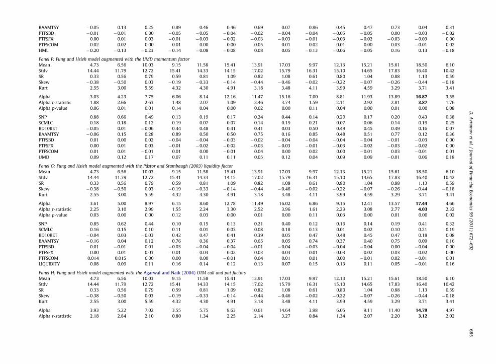
BAAMTSY �0.05 0.13 0.25 0.89 0.46 0.46 0.69 0.07 0.86 0.45 0.47 0.73 0.04 0.31

PTFSBD �0.01 �0.01 0.00 �0.05 �0.05 �0.04 �0.02 �0.04 �0.04 �0.05 �0.05 0.00 �0.03 �0.02

PTFSFX 0.00 0.01 0.03 �0.01 �0.03 �0.02 �0.03 �0.03 �0.01 �0.03 �0.02 �0.03 �0.03 0.00

PTFSCOM 0.02 0.02 0.00 0.01 0.00 0.00 0.05 0.01 0.02 0.01 0.00 0.03 �0.01 0.02

HML �0.20 �0.13 �0.23 �0.14 �0.08 �0.08 0.08 0.05 �0.13 �0.06 �0.05 0.16 0.13 �0.18

Panel F: Fung and Hsieh model augmented with the UMD momentum factor

Mean 4.73 6.56 10.03 9.15 11.58 15.41 13.91 17.03 9.97 12.13 15.21 15.61 18.50 6.10

Stdv 14.44 11.79 12.72 15.41 14.33 14.15 17.02 15.79 16.31 15.10 14.65 17.83 16.40 10.42

SR 0.33 0.56 0.79 0.59 0.81 1.09 0.82 1.08 0.61 0.80 1.04 0.88 1.13 0.59

Skew �0.38 �0.50 0.03 �0.19 �0.33 �0.14 �0.44 �0.46 �0.02 �0.22 �0.07 �0.26 �0.44 �0.18

Kurt 2.55 3.00 5.59 4.32 4.30 4.91 3.18 3.48 4.11 3.99 4.59 3.29 3.71 3.41

Alpha 3.03 4.23 7.75 6.06 8.14 12.16 11.47 15.16 7.00 8.81 11.93 13.89 16.87 3.55

Alpha t-statistic 1.88 2.66 2.63 1.48 2.07 3.09 2.46 3.74 1.59 2.11 2.92 2.81 3.87 1.76

Alpha p-value 0.06 0.01 0.01 0.14 0.04 0.00 0.02 0.00 0.11 0.04 0.00 0.01 0.00 0.08

SNP 0.88 0.66 0.49 0.13 0.19 0.17 0.24 0.44 0.14 0.20 0.17 0.20 0.43 0.38

SCMLC 0.18 0.18 0.12 0.19 0.07 0.07 0.14 0.19 0.21 0.07 0.06 0.14 0.19 0.25

BD10RET �0.05 0.01 �0.06 0.44 0.48 0.41 0.41 0.03 0.50 0.49 0.45 0.49 0.16 0.07

BAAMTSY �0.06 0.15 0.28 0.89 0.50 0.50 0.75 0.16 0.85 0.48 0.51 0.77 0.12 0.36

PTFSBD 0.01 0.00 0.02 �0.04 �0.04 �0.03 �0.02 �0.04 �0.04 �0.04 �0.04 �0.01 �0.03 0.00

PTFSFX 0.00 0.01 0.03 �0.01 �0.02 �0.02 �0.03 �0.03 �0.01 �0.03 �0.02 �0.03 �0.02 0.00

PTFSCOM 0.01 0.01 �0.01 0.01 0.00 �0.01 0.04 0.00 0.02 0.00 �0.01 0.03 �0.01 0.01

UMD 0.09 0.12 0.17 0.07 0.11 0.11 0.05 0.12 0.04 0.09 0.09 �0.01 0.06 0.18

Panel G: Fung and Hsieh model augmented with the Pastor and Stambaugh (2003) liquidity factor

Mean 4.73 6.56 10.03 9.15 11.58 15.41 13.91 17.03 9.97 12.13 15.21 15.61 18.50 6.10

Stdv 14.44 11.79 12.72 15.41 14.33 14.15 17.02 15.79 16.31 15.10 14.65 17.83 16.40 10.42

SR 0.33 0.56 0.79 0.59 0.81 1.09 0.82 1.08 0.61 0.80 1.04 0.88 1.13 0.59

Skew �0.38 �0.50 0.03 �0.19 �0.33 �0.14 �0.44 �0.46 �0.02 �0.22 �0.07 �0.26 �0.44 �0.18

Kurt 2.55 3.00 5.59 4.32 4.30 4.91 3.18 3.48 4.11 3.99 4.59 3.29 3.71 3.41

Alpha 3.61 5.00 8.97 6.15 8.60 12.78 11.49 16.02 6.86 9.15 12.41 13.57 17.44 4.66

Alpha t-statistic 2.25 3.10 2.99 1.55 2.24 3.30 2.52 3.96 1.61 2.23 3.08 2.77 4.03 2.32

Alpha p-value 0.03 0.00 0.00 0.12 0.03 0.00 0.01 0.00 0.11 0.03 0.00 0.01 0.00 0.02

SNP 0.85 0.62 0.44 0.10 0.15 0.13 0.21 0.40 0.12 0.16 0.14 0.19 0.41 0.32

SCMLC 0.16 0.15 0.10 0.11 0.01 0.03 0.08 0.18 0.13 0.01 0.02 0.10 0.21 0.19

BD10RET �0.04 0.03 �0.03 0.42 0.47 0.41 0.39 0.05 0.47 0.48 0.45 0.47 0.18 0.08

BAAMTSY �0.16 0.04 0.12 0.76 0.36 0.37 0.65 0.05 0.74 0.37 0.40 0.75 0.09 0.16

PTFSBD 0.01 �0.01 0.01 �0.03 �0.04 �0.04 �0.01 �0.04 �0.03 �0.04 �0.04 0.00 �0.04 0.00

PTFSFX 0.00 0.01 0.03 �0.01 �0.03 �0.02 �0.03 �0.03 �0.01 �0.03 �0.02 �0.03 �0.02 0.00

PTFSCOM 0.014 0.015 0.00 0.00 0.00 �0.01 0.04 0.01 0.01 0.00 �0.01 0.02 �0.01 0.01

LIQUIDITY 0.08 0.09 0.11 0.16 0.14 0.12 0.13 0.07 0.15 0.13 0.11 0.05 �0.01 0.16

Panel H: Fung and Hsieh model augmented with the Agarwal and Naik (2004) OTM call and put factors

Mean 4.73 6.56 10.03 9.15 11.58 15.41 13.91 17.03 9.97 12.13 15.21 15.61 18.50 6.10

Stdv 14.44 11.79 12.72 15.41 14.33 14.15 17.02 15.79 16.31 15.10 14.65 17.83 16.40 10.42

SR 0.33 0.56 0.79 0.59 0.81 1.09 0.82 1.08 0.61 0.80 1.04 0.88 1.13 0.59

Skew �0.38 �0.50 0.03 �0.19 �0.33 �0.14 �0.44 �0.46 �0.02 �0.22 �0.07 �0.26 �0.44 �0.18

Kurt 2.55 3.00 5.59 4.32 4.30 4.91 3.18 3.48 4.11 3.99 4.59 3.29 3.71 3.41

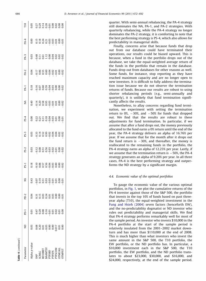
Alpha 3.93 5.22 7.02 3.55 5.75 9.63 10.61 14.64 3.98 6.05 9.11 11.40 14.79 4.97

Alpha t-statistic 2.18 2.84 2.10 0.80 1.34 2.25 2.14 3.27 0.84 1.34 2.07 2.20 3.12 2.02

D.

Av

ram

ov

eta

l./

Jou

rna

lo

fFin

an

cial

Eco

no

mics

99

(20

11

)6

72

–6

92

68

5

Ta

ble

4(c

on

tin

ued

)

Pa

ram

ete

rN

DP

D-1

PD

-2N

SP

S-1

PS

-2P

S-3

PS

-4N

AP

A-1

PA

-2P

A-3

PA

-4T

10

Alp

ha

p-v

alu

e0

.03

0.0

10

.04

0.4

30

.18

0.0

30

.03

0.0

00

.40

0.1

80

.04

0.0

30

.00

0.0

5

SN

P0

.68

0.4

70

.31

�0

.07

�0

.10

�0

.12

�0

.33

0.2

2�

0.1

4�

0.1

6�

0.1

7�

0.4

80

.15

0.2

7

SC

MLC

0.2

00

.20

0.1

50

.19

0.0

80

.08

0.1

40

.21

0.2

00

.07

0.0

60

.11

0.1

80

.29

BD

10

RE

T0

.01

0.0

80

.03

0.5

10

.57

0.5

10

.52

0.1

10

.58

0.6

00

.55

0.6

10

.24

0.1

4

BA

AM

TS

Y�

0.0

30

.16

0.2

40

.93

0.5

60

.56

0.9

90

.18

0.9

50

.59

0.6

01

.12

0.2

10

.28

PT

FSB

D0

.00

�0

.01

0.0

1�

0.0

3�

0.0

4�

0.0

3�

0.0

2�

0.0

4�

0.0

3�

0.0

4�

0.0

40

.00

�0

.03

�0

.01

PT

FSFX

0.0

00

.01

0.0

3�

0.0

1�

0.0

3�

0.0

2�

0.0

4�

0.0

3�

0.0

1�

0.0

3�

0.0

2�

0.0

4�

0.0

30

.00

PT

FSC

OM

0.0

17

0.0

20

.00

0.0

10

.00

�0

.01

0.0

40

.01

0.0

10

.00

�0

.01

0.0

2�

0.0

10

.02

OT

MC

ALL

0.0

10

.01

0.0

00

.00

0.0

00

.00

0.0

20

.00

0.0

00

.00

0.0

00

.02

0.0

00

.00

OT

MP

UT

0.0

00

.00

�0

.01

�0

.01

�0

.02

�0

.02

�0

.02

�0

.01

�0

.02

�0

.02

�0

.02

�0

.02

�0

.01

0.0

0

D. Avramov et al. / Journal of Financial Economics 99 (2011) 672–692686

quarter. With semi-annual rebalancing, the PA-4 strategystill dominates the NA, PA-1, and PA-2 strategies. Withquarterly rebalancing, while the PA-4 strategy no longerdominates the PA-2 strategy, it is comforting to note thatthe best performing strategy is PS-4, which also allows forpredictability in managerial skills.

Finally, concerns arise that because funds that dropout from our database could have terminated theiroperations, our results could be biased upward. This isbecause, when a fund in the portfolio drops out of thedatabase, we take the equal-weighted average return ofthe funds in the portfolio that remain in the database.Funds drop out from databases for other reasons as well.Some funds, for instance, stop reporting as they havereached maximum capacity and are no longer open tonew investors. It is difficult to fully address the termina-tion issue because we do not observe the terminationreturns of funds. Because our results are robust to usingshorter rebalancing periods (e.g., semi-annually andquarterly), it is unlikely that fund termination signifi-cantly affects the results.

Nonetheless, to allay concerns regarding fund termi-nation, we experiment with setting the terminationreturn to 0%, �30%, and �50% for funds that droppedout. We find that the results are robust to theseadjustments for fund termination. In particular, if weassume that after a fund drops out, the money previouslyallocated to the fund earns a 0% return until the end of theyear, the PA-4 strategy delivers an alpha of 16.76% peryear. If we assume that for the month after it drops outthe fund return is �30%, and thereafter, the money isreallocated to the remaining funds in the portfolio, thePA-4 strategy earns an alpha of 12.23% per year. Lastly, ifwe assume that the termination return is �50%, the PA-4strategy generates an alpha of 9.20% per year. In all threecases, PA-4 is the best performing strategy and outper-forms the ND strategy by a significant margin.

4.4. Economic value of the optimal portfolios

To gauge the economic value of the various optimalportfolios, in Fig. 1, we plot the cumulative returns of thePA-4 investor against those of the S&P 500, the portfoliothat invests in the top 10% of funds based on past three-year alpha (T10), the equal-weighted investment in theFung and Hsieh (2004) seven factors (henceforth EW),and the no-predictability dogmatist or ND investor whorules out predictability and managerial skills. We findthat PA-4 strategy performs remarkably well for most ofthe sample period. An investor who invests $10,000 in thePA-4 portfolio at the start of the sample period isrelatively insulated from the 2001–2002 market down-turn and has more than $110,000 at the end of 2008.This is much higher than what investors who invest thesame amount in the S&P 500, the T10 portfolio, theEW portfolio, or the ND portfolio has. In particular, a$10,000 investment each in the S&P 500, the T10portfolio, the EW portfolio, and the ND portfolio trans-lates to about $23,000, $30,000, and $16,000, and$24,000, respectively, at the end of the sample period.

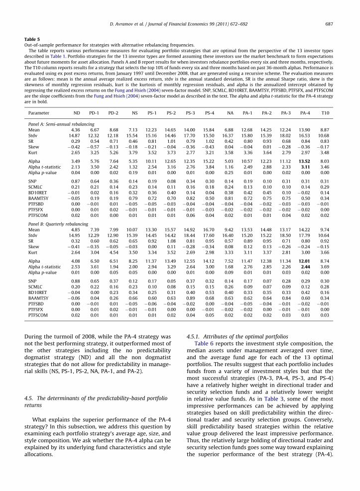
Table 5Out-of-sample performance for strategies with alternative rebalancing frequencies.

The table reports various performance measures for evaluating portfolio strategies that are optimal from the perspective of the 13 investor types

described in Table 1. Portfolio strategies for the 13 investor types are formed assuming these investors use the market benchmark to form expectations

about future moments for asset allocation. Panels A and B report results for when investors rebalance portfolios every six and three months, respectively.

The T10 column reports results for a strategy that selects the top 10% of funds every six and three months based on past 36-month alphas. Performance is

evaluated using ex post excess returns, from January 1997 until December 2008, that are generated using a recursive scheme. The evaluation measures

are as follows: mean is the annual average realized excess return, stdv is the annual standard deviation, SR is the annual Sharpe ratio, skew is the

skewness of monthly regression residuals, kurt is the kurtosis of monthly regression residuals, and alpha is the annualized intercept obtained by

regressing the realized excess returns on the Fung and Hsieh (2004) seven-factor model. SNP, SCMLC, BD10RET, BAAMTSY, PTFSBD, PTFSFX, and PTFSCOM

are the slope coefficients from the Fung and Hsieh (2004) seven-factor model as described in the text. The alpha and alpha t-statistic for the PA-4 strategy

are in bold.

Parameter ND PD-1 PD-2 NS PS-1 PS-2 PS-3 PS-4 NA PA-1 PA-2 PA-3 PA-4 T10

Panel A: Semi-annual rebalancing

Mean 4.36 6.67 8.68 7.13 12.23 14.65 14.00 15.84 6.88 12.68 14.25 12.24 13.90 8.87

Stdv 14.87 12.32 12.18 15.54 15.16 14.46 17.70 15.50 16.37 15.80 15.39 18.02 16.53 10.68

SR 0.29 0.54 0.71 0.46 0.81 1.01 0.79 1.02 0.42 0.80 0.93 0.68 0.84 0.83

Skew �0.42 �0.57 �0.13 �0.18 �0.21 �0.04 �0.36 �0.43 0.04 �0.04 0.01 �0.28 �0.36 �0.17

Kurt 2.65 3.25 5.26 3.79 3.52 3.73 2.77 3.21 3.58 3.36 3.64 2.79 2.97 3.48

Alpha 3.49 5.76 7.64 5.35 10.11 12.65 12.35 15.22 5.03 10.57 12.23 11.12 13.52 8.03

Alpha t-statistic 2.13 3.50 2.42 1.32 2.54 3.16 2.76 3.84 1.16 2.49 2.88 2.33 3.11 3.46

Alpha p-value 0.04 0.00 0.02 0.19 0.01 0.00 0.01 0.00 0.25 0.01 0.00 0.02 0.00 0.00

SNP 0.87 0.64 0.36 0.14 0.19 0.08 0.34 0.30 0.14 0.19 0.10 0.31 0.31 0.31

SCMLC 0.21 0.21 0.14 0.23 0.14 0.11 0.16 0.18 0.24 0.13 0.10 0.10 0.14 0.29

BD10RET �0.01 0.02 0.16 0.32 0.36 0.40 0.14 0.04 0.38 0.42 0.45 0.10 �0.02 0.14

BAAMTSY �0.05 0.19 0.19 0.79 0.72 0.70 0.82 0.50 0.81 0.72 0.75 0.75 0.50 0.34

PTFSBD 0.00 �0.01 0.01 �0.05 �0.05 �0.03 �0.04 �0.04 �0.04 �0.04 �0.02 �0.03 �0.03 �0.01

PTFSFX 0.00 0.01 0.02 �0.01 �0.01 �0.01 �0.01 �0.03 �0.02 �0.02 �0.02 �0.02 �0.02 0.00

PTFSCOM 0.02 0.01 0.00 0.01 0.01 0.01 0.06 0.04 0.02 0.01 0.01 0.04 0.02 0.02

Panel B: Quarterly rebalancing

Mean 4.85 7.39 7.99 10.07 13.30 15.57 14.92 16.70 9.42 13.53 14.48 13.17 14.22 9.74

Stdv 14.95 12.29 12.90 15.39 14.45 14.42 18.44 17.60 16.40 15.20 15.22 18.50 17.79 10.64

SR 0.32 0.60 0.62 0.65 0.92 1.08 0.81 0.95 0.57 0.89 0.95 0.71 0.80 0.92

Skew �0.41 �0.35 �0.05 �0.03 0.00 0.11 �0.28 �0.34 0.08 0.12 0.13 �0.26 �0.24 �0.15

Kurt 2.64 3.04 4.54 3.50 3.34 3.52 2.69 2.98 3.33 3.11 3.37 2.81 3.00 3.66

Alpha 4.08 6.50 6.51 8.25 11.37 13.49 12.55 14.12 7.52 11.47 12.38 11.34 12.01 8.74

Alpha t-statistic 2.53 3.61 1.94 2.00 2.94 3.29 2.64 3.00 1.68 2.76 2.85 2.26 2.44 3.69

Alpha p-value 0.01 0.00 0.05 0.05 0.00 0.00 0.01 0.00 0.09 0.01 0.01 0.03 0.02 0.00

SNP 0.88 0.65 0.37 0.12 0.17 0.05 0.37 0.32 0.14 0.17 0.07 0.28 0.29 0.30

SCMLC 0.20 0.22 0.16 0.23 0.10 0.08 0.15 0.15 0.26 0.09 0.07 0.09 0.12 0.28

BD10RET �0.04 0.00 0.23 0.34 0.25 0.31 0.40 0.53 0.40 0.33 0.35 0.33 0.42 0.16

BAAMTSY �0.06 0.04 0.26 0.66 0.60 0.63 0.89 0.68 0.63 0.62 0.64 0.84 0.60 0.34

PTFSBD 0.00 �0.01 0.01 �0.05 �0.06 �0.04 �0.02 0.00 �0.04 �0.05 �0.04 �0.01 �0.02 �0.01

PTFSFX 0.00 0.01 0.02 �0.01 �0.01 0.00 0.00 �0.01 �0.02 �0.02 0.00 �0.01 �0.01 0.00

PTFSCOM 0.02 0.01 0.01 0.01 0.01 0.02 0.04 0.05 0.02 0.02 0.02 0.03 0.03 0.03

D. Avramov et al. / Journal of Financial Economics 99 (2011) 672–692 687

During the turmoil of 2008, while the PA-4 strategy wasnot the best performing strategy, it outperformed most ofthe other strategies including the no predictabilitydogmatist strategy (ND) and all the non dogmatiststrategies that do not allow for predictability in manage-rial skills (NS, PS-1, PS-2, NA, PA-1, and PA-2).

4.5. The determinants of the predictability-based portfolio

returns

What explains the superior performance of the PA-4strategy? In this subsection, we address this question byexamining each portfolio strategy’s average age, size, andstyle composition. We ask whether the PA-4 alpha can beexplained by its underlying fund characteristics and styleallocations.

4.5.1. Attributes of the optimal portfolios

Table 6 reports the investment style composition, themedian assets under management averaged over time,and the average fund age for each of the 13 optimalportfolios. The results suggest that each portfolio includesfunds from a variety of investment styles but that themost successful strategies (PA-3, PA-4, PS-3, and PS-4)have a relatively higher weight in directional trader andsecurity selection funds and a relatively lower weightin relative value funds. As in Table 3, some of the mostimpressive performances can be achieved by applyingstrategies based on skill predictability within the direc-tional trader and security selection groups. Conversely,skill predictability based strategies within the relativevalue group delivered the least impressive performance.Thus, the relatively large holding of directional trader andsecurity selection funds goes some way toward explainingthe superior performance of the best strategy (PA-4).

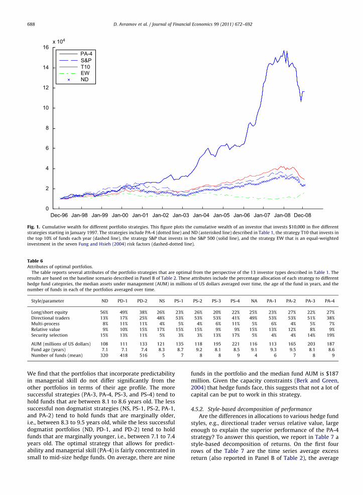
Dec-96 Jan-98 Jan-99 Jan-00 Jan-01 Jan-02 Jan-03 Jan-04 Jan-05 Jan-06 Jan-07 Jan-08 Dec-080

2

4

6

8

10

12

14

16x 104

PA-4S&PT10EWND

Fig. 1. Cumulative wealth for different portfolio strategies. This figure plots the cumulative wealth of an investor that invests $10,000 in five different

strategies starting in January 1997. The strategies include PA-4 (dotted line) and ND (asterisked line) described in Table 1, the strategy T10 that invests in

the top 10% of funds each year (dashed line), the strategy S&P that invests in the S&P 500 (solid line), and the strategy EW that is an equal-weighted

investment in the seven Fung and Hsieh (2004) risk factors (dashed-dotted line).

Table 6Attributes of optimal portfolios.

The table reports several attributes of the portfolio strategies that are optimal from the perspective of the 13 investor types described in Table 1. The

results are based on the baseline scenario described in Panel B of Table 2. These attributes include the percentage allocation of each strategy to different

hedge fund categories, the median assets under management (AUM) in millions of US dollars averaged over time, the age of the fund in years, and the

number of funds in each of the portfolios averaged over time.

Style/parameter ND PD-1 PD-2 NS PS-1 PS-2 PS-3 PS-4 NA PA-1 PA-2 PA-3 PA-4

Long/short equity 56% 49% 38% 26% 23% 26% 20% 22% 25% 23% 27% 22% 27%

Directional traders 13% 17% 25% 48% 53% 53% 53% 41% 49% 53% 53% 51% 38%

Multi-process 8% 11% 11% 4% 5% 4% 6% 11% 5% 6% 4% 5% 7%

Relative value 9% 10% 15% 17% 15% 15% 9% 9% 15% 13% 12% 8% 9%

Security selection 15% 13% 11% 5% 3% 3% 13% 17% 5% 4% 4% 14% 19%

AUM (millions of US dollars) 108 111 133 121 135 118 195 221 116 113 165 203 187

Fund age (years) 7.1 7.1 7.4 8.3 8.7 9.2 8.1 8.5 9.1 9.3 9.5 8.1 8.6

Number of funds (mean) 320 418 516 5 7 8 8 9 4 6 7 8 9

D. Avramov et al. / Journal of Financial Economics 99 (2011) 672–692688

We find that the portfolios that incorporate predictabilityin managerial skill do not differ significantly from theother portfolios in terms of their age profile. The moresuccessful strategies (PA-3, PA-4, PS-3, and PS-4) tend tohold funds that are between 8.1 to 8.6 years old. The lesssuccessful non dogmatist strategies (NS, PS-1, PS-2, PA-1,and PA-2) tend to hold funds that are marginally older,i.e., between 8.3 to 9.5 years old, while the less successfuldogmatist portfolios (ND, PD-1, and PD-2) tend to holdfunds that are marginally younger, i.e., between 7.1 to 7.4years old. The optimal strategy that allows for predict-ability and managerial skill (PA-4) is fairly concentrated insmall to mid-size hedge funds. On average, there are nine

funds in the portfolio and the median fund AUM is $187million. Given the capacity constraints (Berk and Green,2004) that hedge funds face, this suggests that not a lot ofcapital can be put to work in this strategy.

4.5.2. Style-based decomposition of performance

Are the differences in allocations to various hedge fundstyles, e.g., directional trader versus relative value, largeenough to explain the superior performance of the PA-4strategy? To answer this question, we report in Table 7 astyle-based decomposition of returns. On the first fourrows of the Table 7 are the time series average excessreturn (also reported in Panel B of Table 2), the average

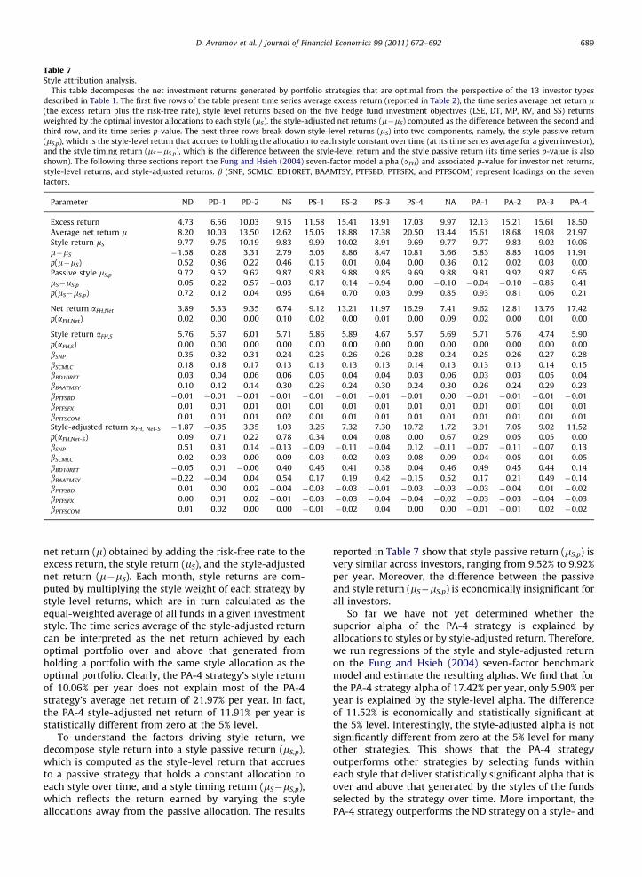
Table 7Style attribution analysis.

This table decomposes the net investment returns generated by portfolio strategies that are optimal from the perspective of the 13 investor types

described in Table 1. The first five rows of the table present time series average excess return (reported in Table 2), the time series average net return m(the excess return plus the risk-free rate), style level returns based on the five hedge fund investment objectives (LSE, DT, MP, RV, and SS) returns

weighted by the optimal investor allocations to each style (mS), the style-adjusted net returns (m�mS) computed as the difference between the second and

third row, and its time series p-value. The next three rows break down style-level returns (mS) into two components, namely, the style passive return

(mS,p), which is the style-level return that accrues to holding the allocation to each style constant over time (at its time series average for a given investor),

and the style timing return (mS�mS,p), which is the difference between the style-level return and the style passive return (its time series p-value is also

shown). The following three sections report the Fung and Hsieh (2004) seven-factor model alpha (aFH) and associated p-value for investor net returns,

style-level returns, and style-adjusted returns. b (SNP, SCMLC, BD10RET, BAAMTSY, PTFSBD, PTFSFX, and PTFSCOM) represent loadings on the seven

factors.

Parameter ND PD-1 PD-2 NS PS-1 PS-2 PS-3 PS-4 NA PA-1 PA-2 PA-3 PA-4

Excess return 4.73 6.56 10.03 9.15 11.58 15.41 13.91 17.03 9.97 12.13 15.21 15.61 18.50

Average net return m 8.20 10.03 13.50 12.62 15.05 18.88 17.38 20.50 13.44 15.61 18.68 19.08 21.97

Style return mS 9.77 9.75 10.19 9.83 9.99 10.02 8.91 9.69 9.77 9.77 9.83 9.02 10.06

m�mS �1.58 0.28 3.31 2.79 5.05 8.86 8.47 10.81 3.66 5.83 8.85 10.06 11.91

p(m�mS) 0.52 0.86 0.22 0.46 0.15 0.01 0.04 0.00 0.36 0.12 0.02 0.03 0.00

Passive style mS,p 9.72 9.52 9.62 9.87 9.83 9.88 9.85 9.69 9.88 9.81 9.92 9.87 9.65

mS�mS,p 0.05 0.22 0.57 �0.03 0.17 0.14 �0.94 0.00 �0.10 �0.04 �0.10 �0.85 0.41

p(mS�mS,p) 0.72 0.12 0.04 0.95 0.64 0.70 0.03 0.99 0.85 0.93 0.81 0.06 0.21

Net return aFH,Net 3.89 5.33 9.35 6.74 9.12 13.21 11.97 16.29 7.41 9.62 12.81 13.76 17.42

p(aFH,Net) 0.02 0.00 0.00 0.10 0.02 0.00 0.01 0.00 0.09 0.02 0.00 0.01 0.00

Style return aFH,S 5.76 5.67 6.01 5.71 5.86 5.89 4.67 5.57 5.69 5.71 5.76 4.74 5.90

p(aFH,S) 0.00 0.00 0.00 0.00 0.00 0.00 0.00 0.00 0.00 0.00 0.00 0.00 0.00

bSNP 0.35 0.32 0.31 0.24 0.25 0.26 0.26 0.28 0.24 0.25 0.26 0.27 0.28

bSCMLC 0.18 0.18 0.17 0.13 0.13 0.13 0.13 0.14 0.13 0.13 0.13 0.14 0.15

bBD10RET 0.03 0.04 0.06 0.06 0.05 0.04 0.04 0.03 0.06 0.03 0.03 0.05 0.04

bBAATMSY 0.10 0.12 0.14 0.30 0.26 0.24 0.30 0.24 0.30 0.26 0.24 0.29 0.23

bPTFSBD �0.01 �0.01 �0.01 �0.01 �0.01 �0.01 �0.01 �0.01 0.00 �0.01 �0.01 �0.01 �0.01

bPTFSFX 0.01 0.01 0.01 0.01 0.01 0.01 0.01 0.01 0.01 0.01 0.01 0.01 0.01

bPTFSCOM 0.01 0.01 0.01 0.02 0.01 0.01 0.01 0.01 0.01 0.01 0.01 0.01 0.01

Style-adjusted return aFH, Net-S �1.87 �0.35 3.35 1.03 3.26 7.32 7.30 10.72 1.72 3.91 7.05 9.02 11.52

p(aFH,Net-S) 0.09 0.71 0.22 0.78 0.34 0.04 0.08 0.00 0.67 0.29 0.05 0.05 0.00

bSNP 0.51 0.31 0.14 �0.13 �0.09 �0.11 �0.04 0.12 �0.11 �0.07 �0.11 �0.07 0.13

bSCMLC 0.02 0.03 0.00 0.09 �0.03 �0.02 0.03 0.08 0.09 �0.04 �0.05 �0.01 0.05

bBD10RET �0.05 0.01 �0.06 0.40 0.46 0.41 0.38 0.04 0.46 0.49 0.45 0.44 0.14

bBAATMSY �0.22 �0.04 0.04 0.54 0.17 0.19 0.42 �0.15 0.52 0.17 0.21 0.49 �0.14

bPTFSBD 0.01 0.00 0.02 �0.04 �0.03 �0.03 �0.01 �0.03 �0.03 �0.03 �0.04 0.01 �0.02

bPTFSFX 0.00 0.01 0.02 �0.01 �0.03 �0.03 �0.04 �0.04 �0.02 �0.03 �0.03 �0.04 �0.03

bPTFSCOM 0.01 0.02 0.00 0.00 �0.01 �0.02 0.04 0.00 0.00 �0.01 �0.01 0.02 �0.02

D. Avramov et al. / Journal of Financial Economics 99 (2011) 672–692 689

net return (m) obtained by adding the risk-free rate to theexcess return, the style return (mS), and the style-adjustednet return (m�mS). Each month, style returns are com-puted by multiplying the style weight of each strategy bystyle-level returns, which are in turn calculated as theequal-weighted average of all funds in a given investmentstyle. The time series average of the style-adjusted returncan be interpreted as the net return achieved by eachoptimal portfolio over and above that generated fromholding a portfolio with the same style allocation as theoptimal portfolio. Clearly, the PA-4 strategy’s style returnof 10.06% per year does not explain most of the PA-4strategy’s average net return of 21.97% per year. In fact,the PA-4 style-adjusted net return of 11.91% per year isstatistically different from zero at the 5% level.

To understand the factors driving style return, wedecompose style return into a style passive return (mS,p),which is computed as the style-level return that accruesto a passive strategy that holds a constant allocation toeach style over time, and a style timing return (mS�mS,p),which reflects the return earned by varying the styleallocations away from the passive allocation. The results

reported in Table 7 show that style passive return (mS,p) isvery similar across investors, ranging from 9.52% to 9.92%per year. Moreover, the difference between the passiveand style return (mS�mS,p) is economically insignificant forall investors.

So far we have not yet determined whether thesuperior alpha of the PA-4 strategy is explained byallocations to styles or by style-adjusted return. Therefore,we run regressions of the style and style-adjusted returnon the Fung and Hsieh (2004) seven-factor benchmarkmodel and estimate the resulting alphas. We find that forthe PA-4 strategy alpha of 17.42% per year, only 5.90% peryear is explained by the style-level alpha. The differenceof 11.52% is economically and statistically significant atthe 5% level. Interestingly, the style-adjusted alpha is notsignificantly different from zero at the 5% level for manyother strategies. This shows that the PA-4 strategyoutperforms other strategies by selecting funds withineach style that deliver statistically significant alpha that isover and above that generated by the styles of the fundsselected by the strategy over time. More important, thePA-4 strategy outperforms the ND strategy on a style- and

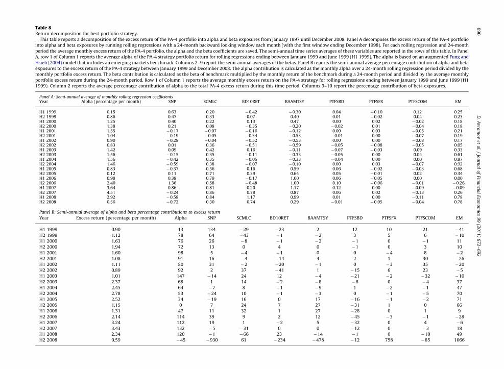
Table 8Return decomposition for best portfolio strategy.

This table reports a decomposition of the excess return of the PA-4 portfolio into alpha and beta exposures from January 1997 until December 2008. Panel A decomposes the excess return of the PA-4 portfolio

into alpha and beta exposures by running rolling regressions with a 24-month backward looking window each month (with the first window ending December 1998). For each rolling regression and 24-month

period the average monthly excess return of the PA-4 portfolio, the alpha and the beta coefficients are saved. The semi-annual time series averages of these variables are reported in the rows of this table. In Panel

A, row 1 of Column 1 reports the average alpha of the PA-4 strategy portfolio return for rolling regressions ending between January 1999 and June 1999 (H1 1999). The alpha is based on an augmented Fung and

Hsieh (2004) model that includes an emerging markets benchmark. Columns 2–9 report the semi-annual averages of the betas. Panel B reports the semi-annual average percentage contribution of alpha and beta

exposures to the excess return of the PA-4 strategy between January 1999 and December 2008. The alpha contribution is calculated as the monthly alpha over a 24-month rolling regression period divided by the

monthly portfolio excess return. The beta contribution is calculated as the beta of benchmark multiplied by the monthly return of the benchmark during a 24-month period and divided by the average monthly

portfolio excess return during the 24-month period. Row 1 of Column 1 reports the average monthly excess return on the PA-4 strategy for rolling regressions ending between January 1999 and June 1999 (H1

1999). Column 2 reports the average percentage contribution of alpha to the total PA-4 excess return during this time period. Columns 3–10 report the percentage contribution of beta exposures.

Panel A: Semi-annual average of monthly rolling regression coefficientsYear Alpha (percentage per month) SNP SCMLC BD10RET BAAMTSY PTFSBD PTFSFX PTFSCOM EM

H1 1999 0.15 0.63 0.20 �0.42 �0.30 0.04 �0.10 0.12 0.25H2 1999 0.86 0.47 0.33 0.07 0.40 0.01 �0.02 0.04 0.23H1 2000 1.25 0.40 0.22 0.13 0.47 0.00 0.02 �0.02 0.18H2 2000 1.38 0.21 0.08 �0.35 �0.20 �0.02 0.01 �0.04 0.18H1 2001 1.55 �0.17 �0.07 �0.16 �0.12 0.00 0.03 �0.05 0.21H2 2001 1.04 �0.19 �0.05 �0.34 �0.53 �0.01 0.00 �0.07 0.19H1 2002 0.90 �0.28 �0.04 �0.52 �0.53 0.00 0.00 �0.08 0.17H2 2002 0.83 0.01 0.36 �0.51 �0.59 �0.05 �0.08 �0.05 0.05H1 2003 1.42 0.09 0.42 0.16 �0.11 �0.07 �0.03 0.09 0.33H2 2003 1.56 �0.15 0.35 �0.11 �0.33 �0.05 0.00 0.04 0.61H1 2004 1.56 �0.42 0.35 �0.06 �0.33 �0.04 0.00 0.00 0.87H2 2004 1.46 �0.59 0.38 �0.07 �0.10 0.00 0.03 �0.07 0.92H1 2005 0.83 �0.37 0.56 0.16 0.59 0.06 �0.02 �0.03 0.68H2 2005 0.12 0.11 0.71 0.39 0.64 0.05 �0.01 0.02 0.34H1 2006 0.98 0.38 0.79 �0.17 1.00 0.06 �0.05 0.00 0.00H2 2006 2.40 1.36 0.58 �0.48 1.00 0.10 �0.06 �0.01 �0.26H1 2007 3.64 0.86 0.81 0.20 1.17 0.12 0.00 �0.09 �0.09H2 2007 4.51 �0.24 0.86 0.78 0.87 0.06 0.02 �0.13 0.26H1 2008 2.92 �0.58 0.84 1.17 0.99 0.01 0.00 �0.11 0.78H2 2008 0.56 �0.72 0.30 0.74 0.29 �0.01 �0.05 �0.04 0.78

Panel B: Semi-annual average of alpha and beta percentage contributions to excess return

Year Excess return (percentage per month) Alpha SNP SCMLC BD10RET BAAMTSY PTFSBD PTFSFX PTFSCOM EM

H1 1999 0.90 13 134 �29 �23 2 12 10 21 �41

H2 1999 1.12 78 64 �43 �1 �2 3 5 6 �10

H1 2000 1.63 76 26 �8 �1 �2 �1 0 �1 11

H2 2000 1.94 72 13 0 4 0 �1 0 3 10

H1 2001 1.60 98 5 �4 �1 0 0 �4 8 �2

H2 2001 1.08 91 16 �4 �14 4 2 1 30 �26

H1 2002 1.11 80 31 �2 �20 �1 0 �3 35 �20

H2 2002 0.89 92 2 37 �41 1 �15 6 23 �5

H1 2003 1.01 147 �14 24 12 �4 �21 �2 �32 �10

H2 2003 2.37 68 1 14 �2 �8 �6 0 �4 37

H1 2004 2.45 64 �7 8 �1 �9 1 �2 �1 47

H2 2004 2.78 53 �24 10 �1 �3 0 �1 �5 70

H1 2005 2.52 34 �19 16 0 17 �16 �1 �2 71

H2 2005 1.15 0 7 24 7 27 �31 1 0 66

H1 2006 1.31 47 11 32 1 27 �28 0 1 9

H2 2006 2.14 114 39 9 2 12 �45 �3 �1 �28

H1 2007 3.24 112 19 1 �2 5 �32 0 4 �6

H2 2007 3.43 132 �5 �31 0 0 �12 0 �3 18

H1 2008 2.34 120 �1 �66 23 �14 �1 0 �10 49

H2 2008 0.59 �45 �930 61 �234 �478 �12 758 �85 1066

D.

Av

ram

ov

eta

l./

Jou

rna

lo

fFin

an

cial

Eco

no

mics

99

(20

11

)6

72

–6

92

69

0

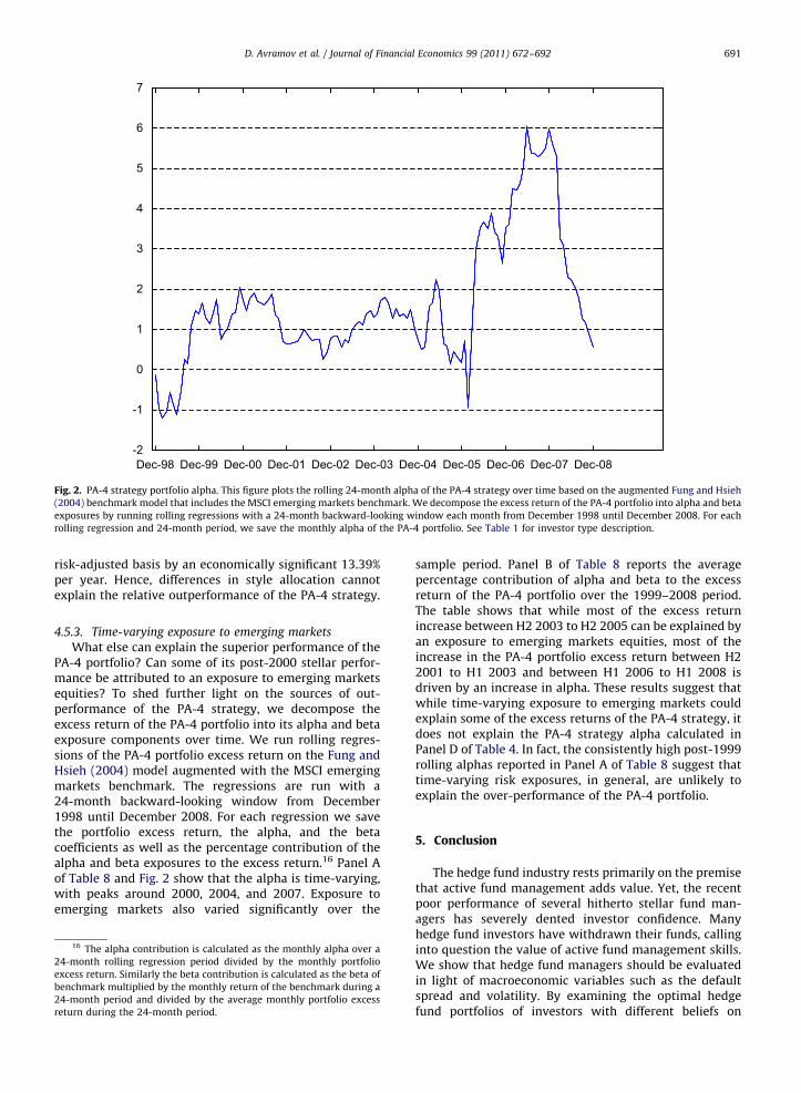
Dec-98 Dec-99 Dec-00 Dec-01 Dec-02 Dec-03 Dec-04 Dec-05 Dec-06 Dec-07 Dec-08-2

-1

0

1

2

3

4

5

6

7

Fig. 2. PA-4 strategy portfolio alpha. This figure plots the rolling 24-month alpha of the PA-4 strategy over time based on the augmented Fung and Hsieh

(2004) benchmark model that includes the MSCI emerging markets benchmark. We decompose the excess return of the PA-4 portfolio into alpha and beta

exposures by running rolling regressions with a 24-month backward-looking window each month from December 1998 until December 2008. For each

rolling regression and 24-month period, we save the monthly alpha of the PA-4 portfolio. See Table 1 for investor type description.

D. Avramov et al. / Journal of Financial Economics 99 (2011) 672–692 691

risk-adjusted basis by an economically significant 13.39%per year. Hence, differences in style allocation cannotexplain the relative outperformance of the PA-4 strategy.

4.5.3. Time-varying exposure to emerging markets

What else can explain the superior performance of thePA-4 portfolio? Can some of its post-2000 stellar perfor-mance be attributed to an exposure to emerging marketsequities? To shed further light on the sources of out-performance of the PA-4 strategy, we decompose theexcess return of the PA-4 portfolio into its alpha and betaexposure components over time. We run rolling regres-sions of the PA-4 portfolio excess return on the Fung andHsieh (2004) model augmented with the MSCI emergingmarkets benchmark. The regressions are run with a24-month backward-looking window from December1998 until December 2008. For each regression we savethe portfolio excess return, the alpha, and the betacoefficients as well as the percentage contribution of thealpha and beta exposures to the excess return.16 Panel Aof Table 8 and Fig. 2 show that the alpha is time-varying,with peaks around 2000, 2004, and 2007. Exposure toemerging markets also varied significantly over the

16 The alpha contribution is calculated as the monthly alpha over a

24-month rolling regression period divided by the monthly portfolio

excess return. Similarly the beta contribution is calculated as the beta of

benchmark multiplied by the monthly return of the benchmark during a

24-month period and divided by the average monthly portfolio excess

return during the 24-month period.

sample period. Panel B of Table 8 reports the averagepercentage contribution of alpha and beta to the excessreturn of the PA-4 portfolio over the 1999–2008 period.The table shows that while most of the excess returnincrease between H2 2003 to H2 2005 can be explained byan exposure to emerging markets equities, most of theincrease in the PA-4 portfolio excess return between H22001 to H1 2003 and between H1 2006 to H1 2008 isdriven by an increase in alpha. These results suggest thatwhile time-varying exposure to emerging markets couldexplain some of the excess returns of the PA-4 strategy, itdoes not explain the PA-4 strategy alpha calculated inPanel D of Table 4. In fact, the consistently high post-1999rolling alphas reported in Panel A of Table 8 suggest thattime-varying risk exposures, in general, are unlikely toexplain the over-performance of the PA-4 portfolio.

5. Conclusion

The hedge fund industry rests primarily on the premisethat active fund management adds value. Yet, the recentpoor performance of several hitherto stellar fund man-agers has severely dented investor confidence. Manyhedge fund investors have withdrawn their funds, callinginto question the value of active fund management skills.We show that hedge fund managers should be evaluatedin light of macroeconomic variables such as the defaultspread and volatility. By examining the optimal hedgefund portfolios of investors with different beliefs on

D. Avramov et al. / Journal of Financial Economics 99 (2011) 672–692692

managerial skills and predictability, we find that incor-porating predictability in managerial skills is important informing optimal portfolios of hedge funds. The key featureof our model is that predictability is based on the defaultspread and the VIX. The strategy that allows for predict-ability in managerial alpha, fund betas, and benchmarkreturns outperforms ex post those strategies that excludepredictability altogether or allow for predictability inbetas and benchmark risk premia only. Our performanceattribution analysis shows that the strategy outperformsother portfolio strategies by selecting funds that generatestatistically significant alpha. Its relative outperformancecannot simply be explained by the styles of the fundsselected by the strategy over time. Our results are robustto various adjustments for backfill bias, incubation bias,illiquidity, fund closure, realistic rebalancing horizons,and alternative benchmark models.

References

Ackermann, C., McEnally, R., Ravenscraft, D., 1999. The performance ofhedge funds: risk, return and incentives. Journal of Finance 54,833–874.

Agarwal, V., Daniel, N., Naik, N.Y., 2009. Flow, performance, andmanagerial incentives in the hedge fund industry. Journal of Finance64, 2221–2256.

Agarwal, V., Naik, N.Y., 2000. Multi-period performance persistenceanalysis of hedge funds. Journal of Financial and QuantitativeAnalysis 53, 327–342.

Agarwal, V., Naik, N.Y., 2004. Risk and portfolio decisions involvinghedge funds. Review of Financial Studies 17, 63–98.

Aggarwal, R.K., Jorion, P., 2010. The performance of emerging hedgefunds and managers. Journal of Financial Economics 96, 238–256.

Avramov, D., 2004. Stock return predictability and asset pricing models.Review of Financial Studies 17, 699–738.

Avramov, D., Chordia, T., 2006a. Asset pricing models and financialmarket anomalies. Review of Financial Studies 19, 1001–1040.

Avramov, D., Chordia, T., 2006b. Predicting stock returns. Journal ofFinancial Economics 82, 387–415.

Avramov, D., Wermers, R., 2006. Investing in mutual funds when returnsare predictable. Journal of Financial Economics 81, 339–377.

Berk, J., Green, R., 2004. Mutual fund flows and performance in rationalmarkets. Journal of Political Economy 112, 1269–1295.

Brown, S., Goetzmann, W., Ibbotson, R., 1999. Offshore hedge funds:survival and performance, 1989–95. Journal of Business 72, 91–117.

Fama, E., French, K., 1989. Business conditions and expected returns onstocks and bonds. Journal of Financial Economics 19, 3–29.

Fama, E., French, K., 1993. Common risk factors in the returns on stocksand bonds. Journal of Financial Economics 33, 3–56.

Fung, W., Hsieh, D., 1997. Is mean variance analysis applicable to hedgefunds? Economic Letters 62, 53–58

Fung, W., Hsieh, D., 1999. A primer on hedge funds. Journal of EmpiricalFinance 6, 309–331.

Fung, W., Hsieh, D., 2000. Performance characteristics of hedge fundsand CTA funds: natural versus spurious biases. Journal of Financialand Quantitative Analysis 35, 291–307.

Fung, W., Hsieh, D., 2001. The risk in hedge fund strategies: theory andevidence from trend followers. Review of Financial Studies 14,313–341.

Fung, W., Hsieh, D., 2004. Hedge fund benchmarks: a risk basedapproach. Financial Analysts Journal 60, 65–80.

Fung, W., Hsieh, D., 2009. Measurement biases in hedge fundperformance data: an update. Financial Analysts Journal 65, 36–38.

Fung, W., Hsieh, D., Naik, N.Y., Ramadorai, T., 2008. Hedge funds:performance, risk, and capital formation. Journal of Finance 63,1777–1803.

Getmansky, M., Lo, A., Makarov, I., 2004. An econometric model of serialcorrelation and illiquidity of hedge fund returns. Journal of FinancialEconomics 74, 529–610.

Gibson, R., Wang, S., 2010. Hedge fund alphas: do they reflect managerialskills or mere compensation for liquidity risk bearing? Unpublishedworking paper. University of Geneva, Switzerland.

Jagannathan, R., Wang, Z., 1996. The conditional CAPM and the cross-section of stock returns. Journal of Finance 51, 3–53.

Jegadeesh, N., Titman, S., 1993. Returns to buying winners and selling losers:implications for stock market efficiency. Journal of Finance 48, 65–91.

Keim, D., Stambaugh, R., 1986. Predicting returns in the stock and bondmarkets. Journal of Financial Economics 17, 357–390.

Kosowski, R., Naik, N.Y., Teo, M., 2007. Do hedge funds deliver alpha? Abootstrap and Bayesian approach. Journal of Financial Economics 84,229–264.

Levy, H., Markowitz, H.M., 1979. Approximating expected utility by afunction of mean and variance. American Economic Review 69, 308–317.

Lowenstein, R., 2000. When Genius Failed: The Rise and Fall of Long–Term Capital Management. Random House, New York.

Malkiel, B., Saha, A., 2005. Hedge funds: risk and return. FinancialAnalysts Journal 61, 80–88.

Mitchell, M., Pulvino, T., 2001. Characteristics of risk in risk arbitrage.Journal of Finance 56, 2135–2175.

Pastor, L., 2000. Portfolio selection and asset pricing models. Journal ofFinance 55, 179–223.

Pastor, L., Stambaugh, R., 2000. Comparing asset pricing models: aninvestment perspective. Journal of Financial Economics 56, 335–381.

Pastor, L., Stambaugh, R., 2002. Mutual fund performance and seeminglyunrelated assets. Journal of Financial Economics 63, 315–349.

Pastor, L., Stambaugh, R., 2003. Liquidity risk and expected stock returns.Journal of Political Economy 111, 642–685.

Zellner, A., Chetty, V.K., 1965. Prediction and decision problems inregression models from the Bayesian point of view. Journal ofAmerican Statistical Association 60, 608–615.