journal of Financial Economics 99 (2011) 204-215

Contents lists available at ScienceDirect

Journal of Financial Economics

journal homepage: www.elsevier.com/locate/jfec

Markowitz meets Talmud: A combination of sophisticatedand naive diversification strategies^Jim Tua ,Guofu Zhou b>*' Singapore Management University, SingaporebOlin School of Business. Washington University, St. Louis, MO 63)30, USA

A R T I C L E I N F O

Article history:Received 29 June 2009Received in revised form3 February 2010Accepted 7 March 2010Available online 24 August 2010

}EL classification:G11G12

Keywords:Portfolio choiceMean-variance analysisParameter uncertainty

A B S T R A C T

The modern portfolio theory pioneered by Markowitz (1952) is widely used in practiceand extensively taught to MBAs. However, the estimated Markowitz portfolio rule andmost of its extensions not only underperform the naive 1/N rule (that invests equallyacross N assets) in simulations, but also lose money on a risk-adjusted basis in manyreal data sets. In this paper, we propose an optimal combination of the naive 1/N rulewith one of the four sophisticated strategies—the Markowitz rule, the Jorion (1986)rule, the MacKinlay and Pastor (2000) rule, and the Kan and Zhou (2007) rule—as a wayto improve performance. We find that the combined rules not only have a significantimpact in improving the sophisticated strategies, but also outperform the 1/N rule inmost scenarios. Since the combinations are theory-based, our study may be interpretedas reaffirming the usefulness of the Markowitz theory in practice.

© 2010 Elsevier B.V. All rights reserved.

1. Introduction

* We are grateful to Yacine A'it-Sahalia, Doron Avramov, Anil Bera,Henry Cao, Winghong Chan (the AFA-NFA discussant), Frans de Roon(the EFA discussant), Arnaud de Servigny, Victor DeMiguel, DavidDisatnik, Lorenzo Garlappi, Eric Ghysels, William Goetzmann, YufengHan, Bruce Hansen, Harrison Hong, Yongmiao Hong, Jing-zhi Huang (theSMUFSC discussant), Ravi Jagannathan. Raymond Kan, Hong Liu, AndrewLo, Todd Milbourn, tubes Pastor, Eduardo Schwartz, G. William Schwert(the managing editor), Paolo Zaffaroni, Chu Zhang (the CICF discussant),seminar participants at Tsinghua University and Washington University,and participants at 2008 China International Conference in Finance, 2008AsianFA-NFA International Conference, 2008 Singapore ManagementUniversity Finance Summer Camp, 2008 European Finance AssociationMeetings, 2008 Workshop on Advances in Portfolio Optimization atLondon Imperial College Business School, and especially to an anon-ymous referee for insightful and detailed comments that havesubstantially improvedthe paper. Tu acknowledges financial supportfor this project from Singapore Management University Research GrantC207/MSS6B006.

* Corresponding author. Tel.: +1 3149356384.E-mail address: zhou@wustl.edu (G. Zhou).

Although more than half a century has passed sinceMarkowitz's (1952) seminal paper, the mean-variance(MV) framework is still the major model used in practicetoday in asset allocation and active portfolio managementdespite many other models developed by academics.1 Onemain reason is that many real-world issues, such as factorexposures and trading constraints, can be accommodatedeasily within this framework with analytical insights andfast numerical solutions. Another reason is that inter-temporal hedging demand is typically found to be small.However, as is the case with any model, the true modelparameters are unknown and have to be estimated fromthe data, resulting in the well-known parameter uncer-tainty or estimation error problem—the estimated

1 See Grinoid and Kahn (1999), Litterman (2003). and Meucci (2005)for practical applications of the mean-variance framework: and seeBrandt (2009) for a recent survey of the academic literature.

0304-405X/$-see front matter © 2010 Elsevier B.V. All rights reserved,doi: 10.1016/j.jfineco.2010.08.013

]. Tu, C. Zhou /Journal of Financial Economics 99 (2011) 204-215 205

optimal portfolio rule is subject to random errors and canthus be substantially different from the true optimal rule.Brown (1976), Bawa and Klein (1976), Bawa, Brown, andKlein (1979), and Jorion (1986) are examples of earlierwork that provide sophisticated portfolio rules accountingfor parameter uncertainty. Recently, MacKinlay andPastor (2000) and Kan and Zhou (2007) provide moresuch rules.2

In contrast to the above sophisticated strategies,the naive 1/N diversification rule, which invests equallyacross N assets of interest, relies on neither any theory norany data. The rule, attributed to the Talmud by Duchinand Levy (2009), has been known for about 1,500 years,and corresponds to the equal weight portfolio in practice.Brown (1976) seems the first academic study of this rule.Due to estimation errors, Jobson and Korkie (1980) statethat "naive formation rules such as the equal weight rulecan outperform the Markowitz rule." Michaud (2008)further notes that "an equally weighted portfolio mayoften be substantially closer to the true MV optimalitythan an optimized portfolio." With similar conclusions,Duchin and Levy (2009) provide an up-to-date compar-ison of the 1/N rule with the Markowitz rule, andDeMiguel, Garlappi, and Uppal (2009) compare the 1/Nrule further with almost all sophisticated extensions ofthe Markowitz rule. Not only that the naive 1/N invest-ment strategy can perform better than those sophisticatedrules recommended from investment theory, but also, asshown elsewhere and below, most of the Markowitz-typerules do not perform well in real data sets and can evenlose money on a risk-adjusted basis in many cases. Thesefindings raise a serious doubt on the usefulness of theinvestment theory.

To address this problem, we examine two relatedquestions. First, we ask whether any of the foursophisticated rules, namely, the Markowitz rule as wellas its extensions proposed by Jorion (1986), MacKinlayand Pastor (2000), and Kan and Zhou (2007), can becombined with the naive 1/N rule to obtain betterportfolio rules that can perform consistently well. Second,we explore whether some or all of the combination rulescan be sufficiently better so that they can outperform the1/N rule. Positive answers to these two questions areimportant, for they will reaffirm the usefulness of theMarkowitz theory if the theory-based combination rulescan perform consistently well and outperform the non-theory-based 1/N rule. The positive answers are alsopossible based on both economic and statistical intuitions.Economically, a concave utility investor will prefer asuitable average of good and bad performances to either agood or a bad performance randomly, similar to thediversification over two risky assets. Statistically, acombination rule can be interpreted as a shrinkageestimator with the 1 /N rule as the target. As is known in

statistics and in finance (e.g., Jorion, 1986), the shrinkageis a tradeoff between bias and variance. The 1 /N rule isbiased, but has zero variance. In contrast, a sophisticatedrule is usually asymptotically unbiased, but can havesizable variance in small samples. When the 1/N rule iscombined with a sophisticated rule, an increase of theweight on the 1/N rule increases the bias, but decreasesthe variance. The performance of the combination ruledepends on the tradeoff between the bias and thevariance. Hence, the performance of the combination rulecan be improved and maximized by choosing an optimalweight.

We find that the four combination rules are substan-tially better than their sophisticated component rules inalmost all scenarios under our study, and some of thecombination rules outperform the 1/N rule as well, evenwhen the sample size (T) is as small as 120. For example,when T=120, in a three-factor model with 25 assets andwith the annualized pricing errors spreading evenlybetween -2% to 2%, for a mean-variance investor withthe risk aversion coefficient y = 3, the four sophisticatedrules, namely, the Markowitz rule and its extensions ofJorion (1986), MacKinlay and Pastor (2000), and Kan andZhou (2007), have utilities (or risk-adjusted returns) of-81.09%, -7.85%, 1.78%, and 1.61%; two of them arelosing money on a risk-adjusted basis. In contrast, theircorresponding combination rules have utilities of 3.84%,5.79%, 1.86%, and 5.09%. Hence, all the combination rulesare better than their uncombined counterparts, and threeof them improve greatly.3 In comparison with the 1/Nrule, which has a utility of 3.85% and is the best rulebefore implementing combinations, two of the combina-tion rules have significantly higher utilities. When T=240or gets larger, while the 1 /N rule, independent of T, stillhas the same performance, all the other rules improve andmany of them outperform the 1/N rule much moresignificantly.

The methodology of this paper is based on the idea ofcombining portfolio strategies. Jorion (1986), Kan andZhou (2007), DeMiguel, Garlappi, and Uppal (2009), andBrandt, Santa-Clara, and Valkanov (2009) have appliedsimilar ideas in various portfolio problems. In contrast tothese studies, this paper focuses on the combination ofthe 1/N rule with the aforementioned Markowitz-typerules, and on reaffirming the value of the investmenttheory. In addition, from a Bayesian perspective, the ideaof combining portfolio strategies is closely related to theBayesian model averaging approach on portfolio selection,which Pastor and Stambaugh (2000) apply to comparevarious asset pricing models and Avramov (2002) appliesto analyze return predictability under model uncertainty.This paper shows, along with these studies, that it isimportant and valuable to combine portfolio strategies inthe presence of estimation errors.

2 Recent Bayesian studies on the parameter uncertainty problem,such as Pastor (2000), Pastor and Stambaugh (2000), Avramov (2004).Harvey. Liechty, Liechty, and Miiller (2004), Tu and Zhou (2004.forthcoming), and Wang (2005), are reviewed by Fabozzi, Huang, andZhou (2010), and Avramov and Zhou (forthcoming). We focus here onthe classical framework.

3 The MacKinlay and Pastor (2000) rule has excellent performanceeven before implementing any combination. But its combination ruleimproves little. As discussed later, this is not a problem with the ruleitself, but a problem with the lack of a good estimation method forestimating the optimal combination coefficient.

206 J. Tu, C. Zhou /Journal of Financial Economics 99 (2011) 204-215

The remainder of the paper is organized as follows.Section 2 provides the combination rules. Section 3compares them with the 1/N rule and with theiruncombined counterparts based on both simulated andreal data sets. Section 4 concludes.

2. Combining portfolio strategies

In this section, we study the combination of the 1/Nrule with each of the four sophisticated strategies. Foreasier understanding, we first briefly illustrate the generalidea of combining two portfolio rules and then present indetail the four combination rules in the order of theiranalytical tractability.

2.1. Combination of two rules

We consider the following combination of two portfo-lio rules:

where we = 1/v/N is the constant 1/N rule, w is anestimated portfolio rule based on the data, and 8 is thecombination coefficient, 0 < 8 < 1. The 1 /N rule here isapplied to N risky assets of interest.4 The implied portfolioreturn of wc at T+l is RpT+^ = r/r+i +wc'RT-n, where r/r+iis the return on the riskless asset, and RT<., is an N-vectorof excess returns on the N risky assets.5

Assume that the excess returns of the N risky assets areindependent and identically distributed over time, andhave a multivariate normal distribution with mean fi andcovariance matrix E. Then the expected utility of wc is

(2)

where y is the mean-variance investor's relative riskaversion coefficient. Our objective is to find an optimalcombination coefficient 8 so that the following expectedloss is minimized:

i(w*,wc) = L/(w*)-E[l/(wc)], (3)

where U(w*) is the expected utility of the true optimalportfolio rule w* = Z~^u/y. This loss function is standardin the statistical decision theory, and is the criterion thatBrown (1976), Frost and Savarino (1986), Stambaugh(1997), Ter Horst, De Roon, and Werker (2006), DeMiguel,Garlappi, and Uppal (2009), among others, use to evaluateportfolio rules.

The 1/N rule is chosen as the starting point of ourcombinations because it is simple, and yet can performremarkably well when the sample size is small. Moreover,as is well-known in statistics (e.g., Lehmann and Casella,1998), 1/N is one common choice of a good shrinkage

4 If the riskless asset is also included, the 1 /N rule may be adjustedto w, = 1N/(N + l). This, worsening from the earlier 1/N rule slightly,makes an insignificant difference in what follows.

5 Note that the performances of most institutional managers arebenchmarked to an index, say the S&P500. Then the return on theS&P500 index portfolio can be viewed as the riskless asset to apply thesame framework. For active portfolio management with benchmarks,see Grinold and Kahn (1999), for example.

point for improving the estimation of the mean of amultivariate distribution. However, the 1 /N rule makes nouse of any sample information, and will always fail toconverge to the true optimal rule if it does not happen tobe equal to it. In contrast, the combination rule alwaysconverges, and is designed to be better than either the 1 /Nrule or w, theoretically.

In practice, though, the true optimal combinationcoefficient 6 is unknown. What is feasible is only acombination rule based on an estimated optimal 8, whoseperformance will then generally vary over applications.However, since the estimation errors in estimating theoptimal 5, which is one single parameter, are usuallysmall, the estimated optimal combination rule cangenerally improve both the 1/N rule and w in our lateranalysis.

2.2. Combining with the Markowitz rule

The simplest case to start with is to combine the 1/Nrule with the standard maximum likelihood (ML) rule orthe (estimated) Markowitz rule. Let /i and t be thesample mean and covariance matrix of R r+i, then the MLrule is given by WML = t~ fijy. Instead of using WML, weuse a scaled one:

w= lr~1/i, (4)

where i = (T/(T-N-2))t. The scaled w is unbiased andperforms slightly better than WML.

According to (1), the combination rule is

wc = (1 — 8)we+8w. (5)

Then the expected loss associated with wc is (all proofsare in the appendices)

L(w*,wc)= [(l-^)27d +82n2].

where

(6)

TI, = (We-WyiXwe-w*). 7r2 = E[(vv-w*)'£(w-w*)].

Note that 7t, measures the impact from the bias of the 1/Nrule, and n2 measures the impact from the variance of w.Thus, the combination coefficient 8 determines thetradeoff between the bias and the variance. The optimalchoice is easily shown as

71,

7T,+7t2

Summarizing the result, we have

(7)

Proposition 1. // TT, > 0, then there exists an optimal 8",0<c5*<l,such that

L(w*,wc)<min[L(w*,we),L(w*,w)], (8)

i.e., the optimal combination rule wc strictly dominates boththe 1/N rule and w.

The condition TT, > 0 is trivially satisfied in practicebecause the 1/N rule will not be equal to the true optimalrule with probability one. Proposition 1 says that theoptimal combination rule wc indeed provides strict

J. Tu, C. Zhou I Journal of Financial Economics 99 (2011) 204-215 207

improvements over both the 1/N rule and w.6 SupposeTTj =712, then (5* = 1 /2, and the loss of wc will be only one-half of the loss of either the 1/N rule or w. This worksexactly like a diversification over two independent andidentically distributed risky assets.

To estimate 8*. we only need to estimate n-i and 7r2,which can be done as follows:

1

C] N

0)

(10)

where 9 is an estimator of (P = u'Z'^u given by Kan andZhou (2007), and Ci =(T-2)(T-N-2)/((T-N-l)(r-N-4)).The condition of T>N+4 is needed here to ensure theexistence of the second moment of Z~ . Summarizing,we have

Proposition 2. Assume T > N+4. On the combination of the1/N rule with w, wc = (1-d)we + 6w, the estimated optima/one is

where 5 —(10).

with

(11)

and ft 2 given by (9) and

Proposition 2 provides a simple way to optimallycombine the 1/N rule with the unbiased ML rule w. Thiscombination rule is easy to carry out in practice since it isonly a given function of the data. However, due to theerrors in estimating 5*, there is no guarantee that theestimated optimal combination rule, WCML, will always bebetter than either the 1/N rule or w. Nevertheless,in our later simulations, the magnitude of the errors inestimating <5*, though varying over different scenarios, aregenerally small. Hence, w does improve upon w, andcan either outperform the 1/N rule or achieve closeperformances in most scenarios. Therefore, the combina-tion does provide improvements overall. In addition, as Tgoes to infinity, w converges to the true optimalportfolio rule.

2.3. Combining with the Kan and Zhou (2007) rule

Consider now the combination of the 1 /N rule with theKan and Zhou (2007) rule, w"2, which is motivated tominimize the impact of estimation errors via a three-fundportfolio. With r\d ftg as defined in their paper (asestimators of the squared slope of the asymptote to theminimum-variance frontier and the expected excessreturn of the global minimum-variance portfolio), wehave

Proposition 3. Assume T>N+4. On the combination ofthe 1/N rule with the Kan and Zhou (2007) rule, wc =(l-SiJWe + SicW*2, the estimated optimal one is

wCKZ = (l—lfc)we+^fcWKZ, (12)

where <5k = ( f t i— fti3)/(ft!— 2fti3 + ft3) with fti given by (9),and ftn and ft3 given by

TCI

IN] . (13)

(14)

Proposition 3 provides the estimated optimal combi-nation rule that combines the 1/N rule with w*2. Bydesign, it should be better than the 1/N rule if the errors inestimating the true optimal <5k are small and if the 1 /Nrule is not exactly identical to the true optimal portfoliorule. This is indeed often the case in the performanceevaluations in Section 3.

2.4. Combining with thejorion (1986) rule

Consider now the combination of the 1 /N rule with theJorion (1986) rule, wpj, which is motivated from both theshrinkage and Bayesian perspectives. Assume T > N+4 asbefore. The optimal combination coefficient can be solvedanalytically in terms of the moments of wpj,

7ti -(w<.-w*)'.££[wPJ-W']* 7r1-2(we-W)TE[wPJ-W]+E[(wPJ-w«)'£(wPJ-w*)]'

(15)

However, due to the complexity of wpj, the analyticalevaluation of the moments is intractable. In Appendix B,we provide an approximate estimator, <5j, of Sj, so that theestimated optimal combination rule,

wCPJ=(l-<5J)we+<5JwPJ, (16)

can be implemented easily in practice.

2.5. Combining with the MacKinlay and Pastor (2000) rule

In order to provide a more efficient estimator of theexpected returns, MacKinlay and Pastor (2000) utilize anextension of the capital asset pricing model (CAPM):

(17)

6 Proposition 1 can be extended to allow any fixed constant rules,and can be adapted to allow biased estimated rules as well.

where f, is a latent factor. Let fiMP and t be themaximum likelihood estimators of the parameters intheir latent factor model (see Appendix C for the details),then the (estimated) MacKinlay and Pastor portfoliorule is given by the standard Markowitz formula,

wMP = (i;MP)-VMP/y. To optimally combine the 1/N rulewith WMP, we need to evaluate the optimal combinationcoefficient:

TT, -2(we-w*)TE[wMP-vir]+E[(wMP-w*)'Z(wMP-w*)]'

(18)

This requires the evaluation of the expectation termsassociated with WMP. Since it is difficult to obtain themanalytically, we use a Jackknife approach (e.g., Shao and

208 J. 7U C. Zhou /Journal of Financial Economics 99 (2011) 204-215

Tu, 1996) to obtain an estimator, 6m, of 8m, via

(19)

E[(wMP-w*)'I(wMP-w*)J

* T[(wMP-w*)'±(wMP-w*)]

(20)

expected utility, do in general have higher Sharpe ratiosthan their uncombined components.

3. Performance evaluation

In this section, we evaluate the performances of thefour combination rules and compare them with theiruncombined counterparts and the 1 /N rule,- based on bothsimulated data sets (10,000 of them) and real data sets.

where w_, is the (estimated) MacKinlay and Pastor rulewhen the t-th observation (t=l,...,T) is deleted from thedata. Then the estimated optimal combination rule is

wCMP = (l-<5m)we+<5rawMp. (21)

With the preparations thus far, it is ready to assess theperformances of WCMP and other rules in both simulationsand real data sets.

2.6. Alternative combinations and criteria

Before evaluating the combination rules provided above,we conclude this section by discussing some broaderperspectives on the combination methodology.7 First, onvarious ways of combining, what are the gains withcombining more than two rules and with combining tworules not including the 1/N rule? Theoretically, if the trueoptimal combination coefficients are known, combiningmore than two rules must dominate combining any subsetof them. However, the true optimal combination coefficientsare unknown and have to be estimated. As more rules arecombined, more combination coefficients need to beestimated and the estimation errors can grow. Hence,combining more than two rules may not improve theperformance. In addition, combining two rules not includingthe 1/N rule is usually not as good as including the 1/N rule,as done by our approach here. Nevertheless, certain optimalestimation methods might be developed to improve theperformances of the more general combination approaches,which is an interesting subject for future research.

Second, on the objective of combining, what happens ifthe combination is to maximize a different objectivefunction? The Sharpe ratio is such a natural objectivewhich seems at least as popular as the utilities or risk-adjusted returns. When the true parameters are known,maximizing the Sharpe ratio and maximizing the ex-pected utility are equivalent, a well-known fact. However,once the true parameters are unknown, the two aredifferent. In this paper, we focus on maximizing theexpected utility as it is easier to solve than maximizingthe Sharpe ratio because the latter is to maximize a highlynonlinear function of the portfolio weights and there areno closed-form solutions available in the presence ofestimation errors. Interestingly, though, due to theirequivalence in the parameter certainty case, the combina-tion strategies of this paper, designed to maximize the

7 We are grateful to an anonymous referee for these and many otherinsights that help to improve the paper enormously.

3.1. Comparison based on simulated data sets

Following MacKinlay and Pastor (2000), and DeMiguel,Garlappi, and Uppal (2009), we assume first the CAPMmodel with an annual excess return of 8% and an annualstandard deviation of 16% on the market factor. The factorloadings, /?'s. are evenly spread between 0.5 and 1.5. Theresidual variance-covariance matrix is assumed to bediagonal, with the diagonal elements drawn from auniform distribution with a support of [0.10, 0.30] so thatthe cross-sectional average annual idiosyncratic volatilityis 20%. In addition, we make two extensions. First, weexamine not only a case of the risk aversion coefficienty = 3, but also a case of y = 1. Second, we allow nonzeroalphas as well to assess the impact of mispricing on theresults. This seems of practical interest because a givenone-factor model (or any given K-factor models, ingeneral) may not hold exactly in the real world.

Table 1 provides the average expected utilities of thevarious rules over the simulated data sets withoutmispricing and with N=25 assets, where the risk-freerate is set as zero without affecting the relative perfor-mances of different rules. Panel A of the table correspondsto the case studied by DeMiguel, Garlappi, and Uppal(2009) with y = 3. The true expected utility is 4.17 (allutility values are annualized and in percentage points),greater than those from the estimated rules as expecteddue to estimation errors. But the four combination rulesall have better performances than their uncombinedcounterparts, respectively. However, in comparison withthe 1/N rule, which achieves a good value of 3.89, thecombination rules have lower utility values, 1.68, 1.42,2.19, and 3.71, when 7-120. Despite the improvementsover their estimated uncombined counterparts, thecombination rules suffer from estimation errors and stillunderperform the 1 /N rule when T is small.

Why does the 1/N rule perform so well in the abovecase? This is because the assumed data-generatingprocess happens to be in its favor: holding the 1/Nportfolio is roughly equivalent to a 100% investment inthe true optimal portfolio. To see why, we note firstthat the betas are evenly spread between 0.5 and 1 .5, andso the 1/N portfolio should be close to the factor portfolio.Second, under the assumption of no mispricing, the factorportfolio is on the efficient frontier, and hence, the trueoptimal portfolio must be proportional to it. The propor-tion depends on y. With y = 3, the 1 /N portfolio happensto be close to the true optimal portfolio, as evidenced byits utility value of 3.89 that is close to the maximumpossible. It is therefore difficult for any other rules, which

J. Tu, C. Zhou /Journal of Financial Economics 99 (2011) 204-215 209

Table 1Utilities in a one-factor model without mispricing.

This table reports the average utilities (annualized and in percentage points) of a mean-variance investor under various investment rules: the trueoptimal rule, the 1/N rule, the ML rule, the Jorion (1986) rule, the MacKinlay and Pastor (2000) rule, the Kan and Zhou (2007) rule, and the fourcombination rules, with 10,000 sets of sample size T simulated data from a one-factor model with zero mispricing alphas and with N-25 assets. Panels Aand B assume that the risk aversion coefficient y is 3 and 1, respectively.

T

Rules

Panel A: y = 3True1/N

MLJorionMacKinlay-PastorKan-Zhou

w™1

wce!

WCMP

w00

Panel B: •/ = 1

True1/N

MLJorionMacKinlay-PastorKan-Zhou

WCML

wcp)

WCMP

A"2

120

4.173.89

-85.72-12.85

2.11-2.15

1.68

1.42

2.19

3.71

12.506.63

-257.16-38.55

6.33-6.44

1.14

1.28

6.57

6.36

240

4.173.89

-25.81-3.793.00

-0.00

2.95

2.93

3.05

3.77

12.506.63

-77.42-11.38

9.00-0.01

4.79

5.68

9.16

6.70

480

4.173.89

-8.35-0.183.441.13

3.42

3.46

3.48

3.81

12.506.63

-25.05-0.5510.313.38

6.39

6.97

10.49

6.99

960

4.173.89

-1.611.553.651.90

3.60

3.71

3.67

3.85

12.506.63

-4.834.6610.945.69

7.47

7.11

11.09

7.41

3000

4.173.89

2.422.983.792.97

3.81

3.88

3.80

3.91

12.506.63

7.258.9511.378.92

9.50

7.46

10.95

8.78

6000

4.17

3.89

3.303.473.833.47

3.90

3.86

3.83

3.95

12.506.63

9.9110.4211.4810.40

10.62

10.34

11.43

9.97

are estimated from the data, to outperform the 1/N rule inthe above particular case.

However, when y = 1, the 1 /N rule will no longer beclose to the true optimal portfolio. This is also evidentfrom Panel B of Table 1. In this case, the expected utility is12.50 from holding the true optimal portfolio. In contrast,if the 1 IN rule is followed, the expected utility is muchlower: 6.63. Note that, although the 1/N rule is notoptimal, it still outperforms the other rules when 1=120.The reason is that the 1/N rule now still holds correctlythe efficient portfolio, though the proportion is incorrect.In contrast, the other rules depend on the estimatedweights, which approximate the efficient portfolioweights with estimation errors. Nevertheless, WCMP andw have close results to the 1/N rule when T=120, andthey do better than it when Ts240. Overall, thecombination rules improve the performances in this caseas well and they do better in outperforming the 1 /N rulethan previously. After understanding the sensitivity of the1/N rule to y, we assume y = 3 as usual in what follows.

When there is mispricing, Panel A of Table 2 reportsthe results where the annualized mispricing alphas areevenly spread between —2% to 2%. The combination rulesagain generally have better performances than theiruncombined counterparts. Now the 1 /N rule gets not onlythe proportion but also the composition of the optimalportfolio incorrect, since the factor portfolio is no longer

on the efficient frontier. In this case, the expected utilityof the 1/N rule, 3.89, is not close to but is about 40% lessthan the expected utility of the true optimal rule, 6.50.Now the combination rules not only improve, they alsooutperform the 1/N rule more easily than before (Panel Aof Table 1).

For the interest of comparison, we now study how therules perform in a three-factor model. We use the sameassumptions as before, except now we have three factors,whose means and covariance matrix are calibrated basedon the monthly data from July 1963 to August 2007 on themarket factor and Fama-French's (1993) size and book-to-market portfolios. The asset factor loadings are randomlypaired and evenly spread between 0.9 and 1.2 for themarket /?'s, between -0.3 and 1.4 for the size portfolio fi's,and between —0.5 and 0.9 for the book-to-marketportfolio fi's. Panel B of Table 2 provides the results withthe same mispricing distribution as before (Panel A ofTable 2). Once again, the combination rules are generallybetter than their estimated uncombined components.Since the 1/N rule is now far away from being the trueoptimal portfolio, it is outperformed by some of thecombination rules even with T-120. As T increases, thecombination rules perform even better. Overall, combina-tion improves performance, and some combination rulescan outperform the 1/N rule in general. This suggests thatthere is indeed value-added through combining rules and

210 ]. Tu, C.Zhou/Journal of Financial Economics 99 (2011) 204-215

Table 2Utilities in factor models with mispricing.

This table reports the average utilities (annualized and in percentage points) of a mean-variance investor under various investment rules: the trueoptimal rule, the 1/N rule, the ML rule, the Jorion (1986) rule, the MacKinlay and Pastor (2000) rule, the Kan and Zhou (2007) rule, and the fourcombination rules, with N*25 assets for 10,000 sets of sample size T simulated data from a one-factor model (Panel A) and a three-factor model (Panel B),respectively. The annualized mispricing a's are assumed to spread evenly between —2% to 2%. The risk aversion coefficient y is 3.

Rules

Panel A: One-factor modelTrue1/N

MLJorionMacKinlay-PastorKan-Zhou

;,cpl

Panel B: Three-factor model

120

6.503.89

-84.75-12.362.34-2.35

2.022.27

2.41

3.84

240

6.503.89

-23.84-2.993.230.02

3.32

3.703.27

3.95

480

6.503.89

-6.180.953.671.64

3.91

4.02

3.71

4.12

960

6.503.89

0.653.093.883.14

4.433.92

3.90

4.41

3000

6.503.89

4.735.064.025.06

5.384.83

4.02

5.14

6000

6.503.89

5.625.714.065.71

5.825.72

4.04

5.62

True1/N

MLJorionMacKinlay-PastorKan-Zhou

WCML

WCP1

WOTP

WCKZ

14.603.85

-81.09-7.851.781.61

3.84

5.79

1.86

5.09

14.603.85

-17.112.842.665.12

6.15

5.36

2.73

6.06

14.603.85

1.397.653.097.96

8.44

4.17

3.12

7.57

14.603.85

8.52

10.453.3010.45

10.63

9.67

3.30

9.59

14.603.85

12.7612.993.4412.99

13.02

13.02

3.45

12.56

14.603.85

13.6913.753.4813.75

13.76

13.76

3.48

13.58

by using portfolio theory to guide portfolio choice overthe use of the naive 1/N diversification.8

3.2. Other properties of the combinations

In this subsection, we explore two aspects about thecombination rules. First, while the combination rules aredesigned to maximize the expected utility, we alsoexamine their performances in terms of the Sharpe ratio,and provide the standard errors for both the utilities andSharpe ratios of the rules over the simulated data sets.Second, we study the estimation errors of the combina-tion coefficients.

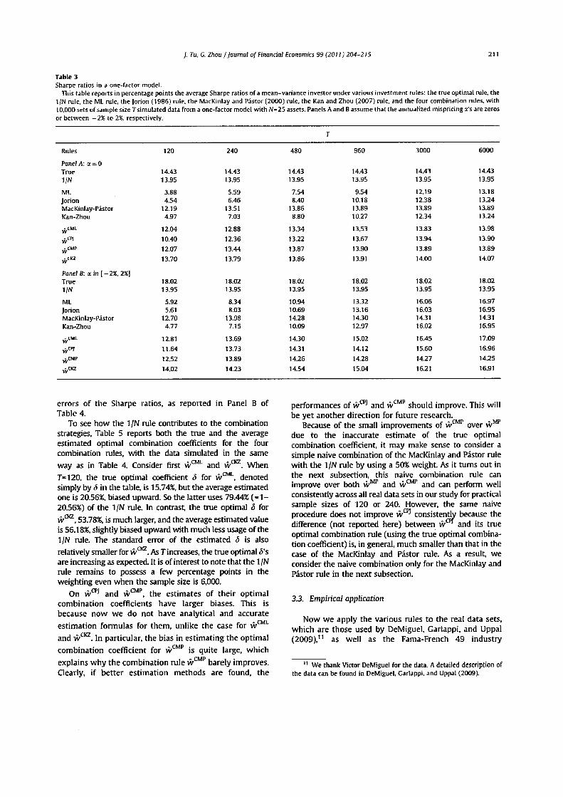
Table 3 provides in percentage points the Sharpe ratiosin the one-factor model. Panel A of the table correspondsto the earlier case studied in Panel A of Table 1. Similar tothe case in utilities, the combination rules generallyimprove the Sharpe ratio substantially, despite thatmaximizing the expected utility may not maximize theSharpe ratio simultaneously in the presence of parameteruncertainty as discussed in Section 2.6. Prior to combin-ing, all the estimated rules, except the MacKinlay andPastor rule, have Sharpe ratios less than 5.0 when T=120.In contrast, the combination rules have Sharpe ratios closeto that of the 1/N rule, 13.95, which in turn is close to the

Sharpe ratio of the true optimal rule, 14.43. As discussedearlier on utilities, the reason why the 1/N rule does sowell is because it is set roughly equal to the true optimalportfolio in this particular simulation design. When somemispricing is allowed (Panel B of Table 3), generallyspeaking, the combination rules again improve, and theyare better than before.9

So far, the combination rules improve significantlyacross various simulation models. Hypothetically, thismight happen with large standard errors in the utilitiesacross data sets. To address this issue. Table 4 reports thestandard errors of all the strategies when the data aredrawn from a three-factor model with the annualizedmispricing a's ranging from —2% to 2%, the casecorresponding to Panel B of Table 2.10 Both the true andthe 1/N rules are data-independent, and so their expectedutilities are the same across data sets. For the estimatedrules, their expected utilities are data-dependent and varyacross data sets with their standard errors ranging from0.29% to 12.37%, when 1=120. The combination rules, ingeneral, have smaller standard errors than their estimatedcomponent rules, especially when the sample size is lessthan 480. Similar results are also true for the standard

8 The same conclusion holds when the number of assets is 50, or in amodel without factor structures. The results are available upon request.

9 Similar results hold, though not reported, in the three-factor modelas well as in the non-factor model.

10 The results in other simulation models are similar, and areomitted for brevity.

]. Tu, C. Zhou /Journal of Financial Economics 99(2011)204-215 211

Table 3Sharps ratios in a one-factor model.

This table reports in percentage points the average Sharpe ratios of a mean-variance investor under various investment rules: the true optimal rule, the1/N rule, the ML rule, the Jorion (1986) rule, the MacKinlay and Pastor (2000) rule, the Kan and Zhou (2007) rule, and the four combination rules, with10.000 sets of sample size T simulated data from a one-factor model with N-25 assets. Panels A and B assume that the annualized mispricing ot's are zerosor between -2% to 2%. respectively.

T

Rules

Panel A: a = 0True1/N

MLJorionMacKinlay-PastorKan-Zhou

WCML

wcp|

WCMP

WCKZ

Panel B: a in [- 2%, 2%]True1/N

MLJorionMacKinlay-PastorKan-Zhou

w™1

wcpj

ACMP

wCKZ

120

14.4313.95

3.88

4.54

12.194.97

12.04

10.40

12.07

13.70

18.0213.95

5.92

5.61

12.704.77

12.81

11.64

12.52

14.02

240

14.43

13.95

5.59

6.46

13.517.03

12.88

12.36

13.44

13.79

18.0213.95

8.34

8.03

13.987.15

13.69

13.73

13.89

14.23

480

14.4313.95

7.54

8.40

13.868.80

13.34

13.22

13.87

13.86

18.0213.95

10.9410.6914.2810.09

14.30

14.31

14.26

14.54

960

14.4313.95

9.54

10.1813.8910.27

13.53

13.67

13.90

13.91

18.0213.95

13.32

13.1614.3012.97

15.02

14.12

14.28

15.04

3000

14.43

13.95

12.19

12.3813.8912.34

13.83

13.94

13.89

14.00

18.0213.95

16.0616.0314.3116.02

16.45

15.60

14.27

16.21

6000

14.4313.95

13.18

13.2413.8913.24

13.98

13.90

13.89

14.07

18.0213.95

16.9716.9514.3116.95

17.09

16.96

14.25

16.91

errors of the Sharpe ratios, as reported in Panel B ofTable 4.

To see how the 1/N rule contributes to the combinationstrategies, Table 5 reports both the true and the averageestimated optimal combination coefficients for the fourcombination rules, with the data simulated in the same

way as in Table 4. Consider first w™1 and w002. WhenT=120, the true optimal coefficient 6 for w™1, denotedsimply by S in the table, is 15.74%, but the average estimatedone is 20.56%, biased upward. So the latter uses 79.44% (=1-20.56%) of the 1/N rule. In contrast, the true optimal S for

w0^, 53.78%, is much larger, and the average estimated valueis 56.18%, slightly biased upward with much less usage of the1/N rule. The standard error of the estimated 5 is also

relatively smaller for WCKZ. As T increases, the true optimal <5'sare increasing as expected. It is of interest to note that the 1/Nrule remains to possess a few percentage points in theweighting even when the sample size is 6,000.

On wcpj and WCMP, the estimates of their optimalcombination coefficients have larger biases. This isbecause now we do not have analytical and accurate

estimation formulas for them, unlike the case for WCML

and WCKZ. In particular, the bias in estimating the optimalcombination coefficient for WCMP is quite large, which

explains why the combination rule WCMP barely improves.Clearly, if better estimation methods are found, the

performances of wcpj and VVCMP should improve. This willbe yet another direction for future research.

Because of the small improvements of WCMP over WMP

due to the inaccurate estimate of the true optimalcombination coefficient, it may make sense to consider asimple naive combination of the MacKinlay and Pastor rulewith the 1/N rule by using a 50% weight. As it turns out inthe next subsection, this naive combination rule canimprove over both WMP and w™1" and can perform wellconsistently across all real data sets in our study for practicalsample sizes of 120 or 240. However, the same naiveprocedure does not improve wcri consistently because thedifference (not reported here) between w0^ and its trueoptimal combination rule (using the true optimal combina-tion coefficient) is, in general, much smaller than that in thecase of the MacKinlay and Pastor rule. As a result, weconsider the naive combination only for the MacKinlay andPastor rule in the next subsection.

3.3. Empirical application

Now we apply the various rules to the real data sets,which are those used by DeMiguel, Garlappi, and Uppal(2009 ),11 as well as the Fama-French 49 industry

11 We thank Victor DeMiguel for the data. A detailed description ofthe data can be found in DeMiguel, Garlappi. and Uppal (2009).

212 J. Tu, C. Zhou /Journal of Financial Economics 99 (2011) 204-215

Table 4Standard errors of utilities and Sharpe ratios.

This table reports the standard errors (in percentage points) of the utilities (Panel A) and the Sharpe ratios (Panel B) for all the strategies with 10,000sets of sample size T simulated data from a three-factor model with N=25 assets. The annualized mispricing a's are assumed to spread evenly between— 2% to 2%. The risk aversion coefficient y is 3.

Rules 120

Panel A: Standard errors of utilitiesTrue 01/N 0

MLJorionMacKinlay-PastorKan-Zhou

wwce>

w™<-.I.CK2

12.373.550.751.44

1.24

0.49

0.67

0.29

240

00

3.291.260.360.72

0.620.37

0.33

0.35

480

00

1.240.610.170.50

0.47

0.31

0.16

0.40

960

00

0.530.330.09032

0.31

0.70

0.08

0.36

3000

00

0.150.130.030.13

0.13

0.13

0.03

0.17

6000

00

0.080.07

0.010.07

0.07

0.07

0.01

0.08

Panel B: Standard errors of Sharp ratiosTrue1/N

MLJorionMacKinlay-PastorKan-Zhou

w™L

wces

w™11

w03

00

4.024.186.874.51

2.44

2.57

6.36

1.66

00

3.012.873.542.82

2.22

2.25

3.38

1.88

00

2.001.841.161.90

1.85

2.28

0.80

1.84

00

1.191.120.271.16

1.12

3.22

0.07

1.30

00

0.430.420.040.42

0.42

0.43

0.04

0.45

00

0.220.220.030.22

0.22

0.22

0.03

0.23

Table 5Combination coefficients.

This table reports in percentage points the true optimal combination coefficients, the average estimated optimal combination coefficients and theirstandard errors (in parentheses) for the four combination strategies. The data are simulated in the same way as in Table 4.

r

Parameters

Panel A: w™*&i>

Panel B: w1*1

Oj

$.

Panel C: w™p

om

Om

Panel D: w™2

5k

ik

120

15.7420.56

(10.87)

27.5635.95

(12.78)

28.5097.02

(1.14)

53.7856.18(6.37)

240

29.9329.38

(13.44)

46.6517.61

(16.41)

42.5497.27

(0.89)

68.0957.37

(7.70)

480

47.5745.16

(12.49)

65.2911.52

(29.55)

56.0698.03

(0.87)

79.8763.49

(7.88)

960

65.1263.73

(7.61)

80.3287.90

(32.63)

66.6299.37

(0.75)

88.3572.26

(6.49)

3000

85.6085.35

(2.05)

93.90100.00

(0.00)

76.25100.00

(0.00)

95.8186.43

(3.09)

6000

92.2792.20

(0.80)

97.17100.00

(0.00)

78.93100.00

(0.00)

97.8492.27

(1.52)

portfolios plus the Fama-French three factors and theearlier Fama-French 25 portfolios plus the Fama-Frenchthree factors.

Given a sample size of T, we use a rolling estimationapproach with two estimation windows of length M=120and 240 months, respectively. In each month t, starting

}. Tu. C. Zhou /Journal of Financial Economics 99 (2011) 204-215 213

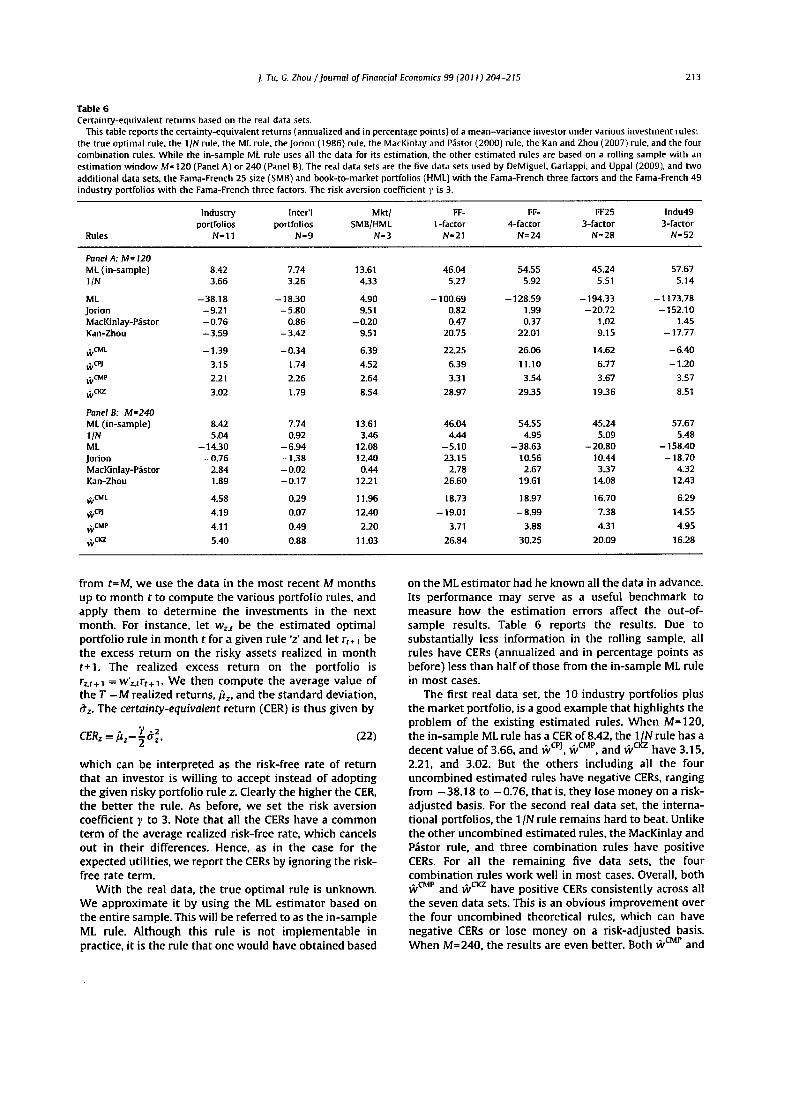
Table 6Certainty-equivalent returns based on the real data sets.

This table reports the certainty-equivalent returns (annualized and in percentage points) of a mean-variance investor under various investment rules:the true optimal rule, the 1/N rule, the ML rule, the Jorion (1986) rule, the MacKinlay and Pastor (2000) rule, the Kan and Zhou (2007) rule, and the fourcombination rules. While the in-sample ML rule uses all the data for its estimation, the other estimated rules are based on a rolling sample with anestimation window M=120 (Panel A) or 240 (Panel B). The real data sets are the five data sets used by DelMiguel, Garlappi. and Uppal (2009), and twoadditional data sets, the Fama-French 25 size (SMB) and book-to-market portfolios (HML) with the Fama-French three factors and the Fama-French 49industry portfolios with the Fama-French three factors. The risk aversion coefficient y is 3.

Rules

Panel A: M-120ML (in-sample)1/N

MLJorionMacKinlay-PastorKan-Zhou

WCMU

wcp)

w™"WCKZ

Panel B: M-240ML (in-sample)1/NMLJorionMacKinlay-PastorKan-Zhou

w™1

w^VVCMP

w00

Industryportfolios

N-ll

8.423.66

-38.18-9.21-0.76-3.59

-1.393.152.213.02

8.425.04

-14.30-0.76

2.841.89

4.584.194.115.40

Inter'lportfolios

N-9

7.743.26

- 1 8.30-5.80

0.86-3.42

-0.341.742.261.79

7.740.92

-6.94-1.38-0.02-0.17

0.290.070.490.88

Mkt/SMB/HML

N-3

13.614.33

4.909.51

-0.209.51

6.394.522.648.54

13.613.46

12.0812.400.44

12.21

11.9612.402.20

11.03

FF-1 -factor

N-21

46.045.27

-100.690.820.47

20.75

22.25

6.393.31

28.97

46.044.44

-5.1023.15

2.7826.60

18.73-19.01

3.7126.84

FF-4-factor

N=24

54.555.92

-128.591.990.37

22.01

26.06

11.103.54

29.35

54.554.95

-38.6310.562.67

19.61

18.97-8.99

3.8830.25

FF253-factor

N-28

45.245.51

-194.33-20.72

1.029.15

14.626.773.67

19.36

45.245.09

-20.8010.44337

14.08

16.707.384.31

20.09

Indu493-factor

N-52

57.675.14

-1173.78-152.10

1.45-17.77

-6.40-1.20

3.578.51

57.675.48

-158.40-18.70

4.3212.43

6.2914.554.95

16.28

from t=M, we use the data in the most recent M monthsup to month t to compute the various portfolio rules, andapply them to determine the investments in the nextmonth. For instance, let w2J be the estimated optimalportfolio rule in month t for a given rule 'z' and let rt+1 bethe excess return on the risky assets realized in monthr+1. The realized excess return on the portfolio isrz,t+\z.trt+i. We then compute the average value ofthe T -M realized returns. fiz, and the standard deviation,ffz. The certainty-equivalent return (CER) is thus given by

(22)

which can be interpreted as the risk-free rate of returnthat an investor is willing to accept instead of adoptingthe given risky portfolio rule z. Clearly the higher the CER,the better the rule. As before, we set the risk aversioncoefficient y to 3. Note that all the CERs have a commonterm of the average realized risk-free rate, which cancelsout in their differences. Hence, as in the case for theexpected utilities, we report the CERs by ignoring the risk-free rate term.

With the real data, the true optimal rule is unknown.We approximate it by using the ML estimator based onthe entire sample. This will be referred to as the in-sampleML rule. Although this rule is not implementable inpractice, it is the rule that one would have obtained based

on the ML estimator had he known all the data in advance.Its performance may serve as a useful benchmark tomeasure how the estimation errors affect the out-of-sample results. Table 6 reports the results. Due tosubstantially less information in the rolling sample, allrules have CERs (annualized and in percentage points asbefore) less than half of those from the in-sample ML rulein most cases.

The first real data set, the 10 industry portfolios plusthe market portfolio, is a good example that highlights theproblem of the existing estimated rules. When M=120,the in-sample ML rule has a CER of 8.42, the 1/N rule has adecent value of 3.66, and wcpj, WCMP, and wcte have 3.15,2.21, and 3.02. But the others including all the fouruncombined estimated rules have negative CERs, rangingfrom —38.18 to -0.76, that is, they lose money on a risk-adjusted basis. For the second real data set, the interna-tional portfolios, the 1 /N rule remains hard to beat. Unlikethe other uncombined estimated rules, the MacKinlay andPastor rule, and three combination rules have positiveCERs. For all the remaining five data sets, the fourcombination rules work well in most cases. Overall, bothWCMP and w02 have positive CERs consistently across allthe seven data sets. This is an obvious improvement overthe four uncombined theoretical rules, which can havenegative CERs or lose money on a risk-adjusted basis.When M=240, the results are even better. Both WCMP and

214 ]. Tu. C. Zhou /Journal of Financial Economics 99 (2011) 204-215

wCKZ now still have positive CERs consistently across allthe seven data sets. Moreover, most of the combinationrules not only improve, but also outperform the 1 /N rulemost of the time.

In short, when applied to the real data sets, thecombination rules generally improve from their uncom-bined Markowitz-type counterparts and can performconsistently well, and some of them can outperform the1 IN rule in most of the cases.

4. Conclusion

The modern portfolio theory pioneered by Markowitz(1952) is widely used in practice and extensively taught toMBAs. However, due to parameter uncertainty or estima-tion errors, many studies show that the naive 1/Ninvestment strategy performs much better than thoserecommended from the theory. Moreover, the existingtheory-based portfolio strategies, except that of MacK-inlay and Pastor (2000), perform poorly when applied tomany real data sets used in our study. These findings raisea serious doubt on the usefulness of the investmenttheory. In this paper, we provide new theory-basedportfolio strategies which are the combinations of thenaive 1/N rule with the sophisticated theory-basedstrategies. We find that the combination rules aresubstantially better than their uncombined counterparts,in general, even when the sample size is small. Inaddition, some of the combination rules can performconsistently well and outperform the 1/N rule signifi-cantly. Overall, our study reaffirms the usefulness of theinvestment theory and shows that combining portfoliorules can potentially add significant value in portfoliomanagement under estimation errors.

Since parameter uncertainty appears in almost everyfinancial decision-making problem, our ideas and resultsmay be applied to various other areas. For example, theymay be applied to turn many practical quantitativeinvesting strategies (e.g., Lo and Patel, 2008) into thosemore robust to estimation errors; they may also beapplied to hedge derivatives optimally in the presenceof parameter uncertainty; or be applied to make optimalcapital structure decisions with unknown investors'expectations and macroeconomic determinants. Whilestudies of these issues go beyond the scope of this paper,they seem interesting topics for future research.

Appendix A. Proofs of propositions and equations

AJ. Proof of Proposition 1

Based on (6), we need only to show

f(S)= (1-<5)27T, +S2TI2 = 7T1-2^7t1 + <52(7t1 +T12) (23)

A.2. Proof of Eq. (10)

In many expectation evaluations below, a key is toapply two equalities about the inverse of the samplecovariance matrix (e.g.. Haff, 1979), i.e., the formulas for

EfZ:1/2!;''^2] and £[r1/2r"1ri~li:1/2]. Expanding outthe quadratic form of 712 into three terms, and applyingthe formulas to the two terms involving w, we have

(24)

Then, plugging the estimator for Q2 into this equationyields the desired claim.

A.3. Proof of Proposition 3

Now, we have

L(w*,wc)=

where w denotes v/2 for brevity. Let a — we— w* andb = w-w*. then the following identity holds:

[(1 -<5)a + <5b]'.£[(l -<5)a + <5b]= (1 -<5)2aTa+2<5(1 -<5)a:rb+<52bTb.

Taking the first-order derivative of this identity, we obtainthe optimal choice of <5,

a'Za-a'ZE[b]&=• (25)

'aTa-2aTE[b]+E[b'Zbr

It is clear that n^ =a'Sa. Let 7^3 = aTE[b] =we'r£[w]-

wf'n-n'E[w]+tiZ-}n. Since E\Z~^] = TZ^ / (T-N-2). wecan estimate n\$ with n\^ as given by (13). Finally, let7t3 = E[b'Ib]. Using Eq. (63) of Kan and Zhou (2007), wecan estimate n3 with #3 as given by (14).

Appendix B. Combining with the Jorion (1986) rule

Eq. (15) follows from (25). To compute £[(rV1 ftP]lwe rewrite

(26)

where d and D are defined accordingly from (26).Inverting this matrix, we have

(fV1 = £~' /d-r"1 DDT"1 /(d2 + dDT"1 D) = 1"' /d-B,(27)

where B is defined as the second term. Since it is relativelysmall, we treat it as a constant. Then, we approximately

evaluate E[(t r^ftP}] as the product of the expectations.Finally, we have from (27) that

satisfies /'(<5*) = 0 and /"(<5*) > 0 at 6*. which are easy toverify. Then the claim follows.

(28)

The first term can be evaluated as in Proposition 3. Thesecond and third terms are trivial. Hence, we can evaluate

approximately E[(ip]'(Zf]r* £(£**)'* frPJ] by treating ±PJ

and fifi as independent variables.

J. Tu, C. Zhou /Journal of Financial Economics 99 (2011) 204-215 215

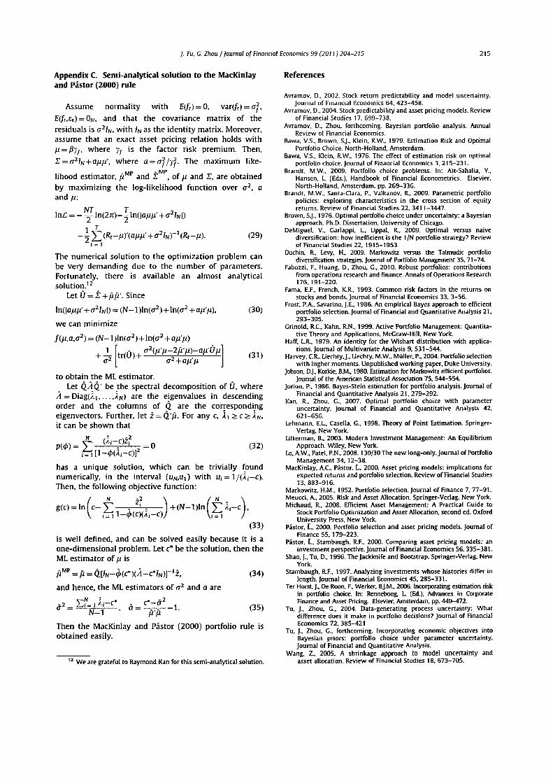
Appendix C. Semi-analytical solution to the MacKinfayand Pastor (2000) rule

Assume normality with £(/",) = 0, var(/t) = <r2,E(ft.£t) = 0N, and that the covariance matrix of theresiduals is er2//v, with /N as the identity matrix. Moreover,assume that an exact asset pricing relation holds withH = j}y!, where yf is the factor risk premium. Then,

r = <T2/N + a/i/i', where a = ffj/y2. The maximum like-

lihood estimator, fiMP and t , of ju and T, are obtainedby maximizing the log-likelihood function over <72, aand fi:

NT T

i

1 (Rt-H). (29)

The numerical solution to the optimization problem canbe very demanding due to the number of parameters.Fortunately, there is available an almost analyticalsolution.12

Let 0 = Z +ftfi'. Since

(30)

(31)

to obtain the ML estimator.Let QAQ' be the spectral decomposition of U, where

/i=Diag(l] IN) are the eigenvalues in descendingorder and the columns of Q are the correspondingeigenvectors. Further, let z = Q'/i. For any c,it can be shown that

we can minimize

f(H,a,a2) = (N-l)ln(o-2)+ln(ff2

= V- q.-c)z2 = o (32)

has a unique solution, which can be trivially foundnumerically, in the interval (UN,U\) with Uj = l/(i,—-c).Then, the following objective function:

/ " z2 A /A- \) = lnlc-]P =—!-̂ )+(N-1)lnl ^Aj-c ,

(33)

is well defined, and can be solved easily because it is aone-dimensional problem. Let c* be the solution, then theML estimator of /i is

z. (34)

(35)

and hence, the ML estimators of a2 and a are

_" ~

c'-aN-l

Then the MacKinlay and Pastor (2000) portfolio rule isobtained easily.

: We are grateful to Raymond Kan for this semi-analytical solution.

References

Avramov, D., 2002. Stock return predictability and model uncertainty.Journal of Financial Economics 64, 423-458.

Avramov. D.. 2004. Stock predictability and asset pricing models. Reviewof Financial Studies 17. 699-738.

Avramov. D.. Zhou, forthcoming. Bayesian portfolio analysis. AnnualReview of Financial Economics.

Bawa. V.S.. Brown, S.J.. Klein. R.W.. 1979. Estimation Risk and OptimalPortfolio Choice. North-Holland. Amsterdam.

Bawa. V.S.. Klein. R.W.. 1976. The effect of estimation risk on optimalportfolio choice. Journal of Financial Economics 3, 215-231.

Brandt, M.W., 2009. Portfolio choice problems. In: Ait-Sahalia. Y.,Hansen, L. (Eds.). Handbook of Financial Econometrics. Elsevier.North-Holland, Amsterdam, pp. 269-336.

Brandt, M.W., Santa-Clara, P., Valkanov, R., 2009. Parametric portfoliopolicies: exploiting characteristics in the cross section of equityreturns. Review of Financial Studies 22. 3411-3447.

Brown, S.J.. 1976. Optimal portfolio choice under uncertainty: a Bayesianapproach. Ph.D. Dissertation, University of Chicago.

DeMiguel, V.. Garlappi. L. Uppal, R.. 2009. Optimal versus naivediversification: how inefficient is the 1/N portfolio strategy? Reviewof Financial Studies 22, 1915-1953

Duchin. R., Levy. H.. 2009. Markowitz versus the Talmudic portfoliodiversification strategies. Journal of Portfolio Management 35, 71-74.

Fabozzi. F.. Huang, D.. Zhou, C., 2010. Robust portfolios: contributionsfrom operations research and finance. Annals of Operations Research176,191-220.

Fama. E.F.. French. K.R., 1993. Common risk factors in the returns onstocks and bonds. Journal of Financial Economics 33, 3-56.

Frost, PA. Savarino, J.E., 1986. An empirical Bayes approach to efficientportfolio selection. Journal of Financial and Quantitative Analysis 21,293-305.

Grinold. R.C.. Kahn, R.N., 1999. Active Portfolio Management: Quantita-tive Theory and Applications. McGraw-Hill, New York.

Haff. L.R.. 1979. An identity for the Wishart distribution with applica-tions. Journal of Multivariate Analysis 9, 531-544.

Harvey, C.R.. Liechty, J.. Liechty, M.W., Muller. P., 2004. Portfolio selectionwith higher moments. Unpublished working paper, Duke University.

Jobson, D.J.. Korkie. B.M., 1980. Estimation for Markowitz efficient portfolios.Journal of the American Statistical Association 75, 544-554.

Jorion. P., 1986. Bayes-Stein estimation for portfolio analysis. Journal ofFinancial and Quantitative Analysis 21, 279-292.

Kan, R., Zhou, G., 2007. Optimal portfolio choice with parameteruncertainty. Journal of Financial and Quantitative Analysis 42,621-656.

Lehmann, E.L, Casella, G., 1998. Theory of Point Estimation. Springer-Verlag, New York.

Litterman, B., 2003. Modern Investment Management: An EquilibriumApproach. Wiley. New York.

Lo, A.W., Patel, P.N., 2008.130/30 The new long-only. Journal of PortfolioManagement 34.12-38.

MacKinlay, A.C., Pastor, L, 2000. Asset pricing models: implications forexpected returns and portfolio selection. Review of Financial Studies13, 883-916.

Markowitz, H.M.. 1952. Portfolio selection. Journal of Finance 7, 77-91.Meucci, A., 2005. Risk and Asset Allocation. Springer-Verlag, New York.Michaud, R., 2008. Efficient Asset Management: A Practical Guide to

Stock Portfolio Optimization and Asset Allocation, second ed. OxfordUniversity Press, New York.

Pastor, L, 2000. Portfolio selection and asset pricing models. Journal ofFinance 55,179-223.

Pastor, L. Stambaugh, R.F., 2000. Comparing asset pricing models: aninvestment perspective. Journal of Financial Economics 56.335-381.

Shao, J., Tu, D., 1996. The Jackknife and Bootstrap. Springer-Verlag, NewYork.

Stambaugh, R.F.. 1997. Analyzing investments whose histories differ inlength. Journal of Financial Economics 45, 285-331.

Ter Horst, J., De Roon, F., Werker, B.J.M.. 2006. Incorporating estimation riskin portfolio choice. In: Renneboog, L (Ed.), Advances in CorporateFinance and Asset Pricing. Elsevier. Amsterdam, pp. 449-472.

Tu. J.. Zhou. G.. 2004. Data-generating process uncertainty: Whatdifference does it make in portfolio decisions? Journal of FinancialEconomics 72. 385-421

Tu, J., Zhou, G., forthcoming. Incorporating economic objectives intoBayesian priors: portfolio choice under parameter uncertainty.Journal of Financial and Quantitative Analysis.

Wang, Z., 2005. A shrinkage approach to model uncertainty andasset allocation. Review of Financial Studies 18. 673-705.