Contents lists available at SciVerse ScienceDirect

Journal of Financial Economics

Journal of Financial Economics 109 (2013) 146–176

0304-40

http://d

$ Thi

paper w

Lamont

Merton

Vermily

Venice,

Interme

Associa

Internat

on Bankn Corr

fax: þ1

E-m1 Te

journal homepage: www.elsevier.com/locate/jfec

How does capital affect bank performance during financialcrises?$

Allen N. Berger a,b,c,n, Christa H.S. Bouwman b,d,1

a University of South Carolina, Moore School of Business, 1705 College Street, Columbia, SC 29208, USAb Wharton Financial Institutions Center, University of Pennsylvania, Philadelphia, PA 19104, USAc Center for Economic Research (CentER)—Tilburg University, PO Box 90153, 5000 LE Tilburg, The Netherlandsd Case Western Reserve University, Weatherhead School of Management, 10900 Euclid Avenue, 362 PBL, Cleveland, OH 44106, USA

a r t i c l e i n f o

Article history:

Received 11 March 2011

Received in revised form

7 May 2012

Accepted 11 December 2012Available online 13 February 2013

JEL classification:

G01

G28

G21

Keywords:

Financial crises

Survival

Market share

Profitability

Banking

5X/$ - see front matter & 2013 Elsevier B.V

x.doi.org/10.1016/j.jfineco.2013.02.008

s is a significantly expanded version of the se

as entitled ‘‘Bank capital, survival and perfo

Black, Maarten Buis, Elena Carletti, Rebel Co

, Steven Ongena, Bruno Parigi, Peter Ritchke

ae, and participants at presentations at the

the European School of Management an

diation (JFI) / Center for Economic Policy Re

tion meeting, the Boston Federal Reserve, th

ional Monetary Fund, the Summer Research

ing and Finance, the University of Kansas S

esponding author at: University of South Ca

803 777 6876.

ail addresses: aberger@moore.sc.edu (A.N. B

l.: þ216 368 3688; fax: þ216 368 6249.

a b s t r a c t

This paper empirically examines how capital affects a bank’s performance (survival and

market share) and how this effect varies across banking crises, market crises, and normal

times that occurred in the US over the past quarter century. We have two main results.

First, capital helps small banks to increase their probability of survival and market share

at all times (during banking crises, market crises, and normal times). Second, capital

enhances the performance of medium and large banks primarily during banking crises.

Additional tests explore channels through which capital generates these effects. Numer-

ous robustness checks and additional tests are performed.

& 2013 Elsevier B.V. All rights reserved.

1. Introduction

The recent financial crisis raises fundamental issuesabout the role of bank equity capital, particularly from thestandpoint of bank survival. Not surprisingly, public

. All rights reserved.

cond part of an earlier pape

rmance around financial cr

le, Bob DeYoung, John Finn

n, Raluca Roman, Katherine

American Finance Associa

d Technology, the Centre

search (CEPR) Conference on

e Philadelphia Federal Reser

Conference in Finance at th

outhwind Finance Conferen

rolina, Moore School of Bu

erger), christa.bouwman@ca

outcries for more bank capital tend to be greater afterfinancial crises, and post-crisis reform proposals tend tofocus on how capital regulation should adapt to preventfuture crises. Various such proposals have been put forthrecently (e.g., Kashyap, Rajan, and Stein, 2008; BIS, 2010;

r, ‘‘Financial crises and bank liquidity creation.’’ A previous version of this

ises.’’ We thank two anonymous referees, Franklin Allen, Nittai Bergman,

erty, Mark Flannery, Xavier Freixas, Paolo Fulghieri, Robert Marquez, Bob

Samolyk, Asani Sarkar, Anjan Thakor, James Thomson, Greg Udell, Todd

tion meeting, the Bank for International Settlements, the University of

de Recerca en Economia Internacional (CREI) / Journal of Financial

Financial Crises at Pompeu Fabra University, the Financial Management

ve, the San Francisco Federal Reserve, the Cleveland Federal Reserve, the

e Indian School of Business in Hyderabad, India, the Unicredit Conference

ce, Erasmus University, and Tilburg University for useful comments.

siness, Columbia, SC 29208, USA. Tel.: þ1 803 576 8440;

se.edu (C.H.S. Bouwman).

A.N. Berger, C.H.S. Bouwman / Journal of Financial Economics 109 (2013) 146–176 147

Acharya, Mehran, and Thakor, 2011; Admati, DeMarzo,Hellwig, and Pfleiderer, 2011; Calomiris and Herring,2011; Hart and Zingales, 2011). An underlying premisein these proposals is that externalities exist due to thesafety net provided to banks and, thus, social efficiencycan be improved by requiring banks to operate with morecapital, especially during financial crises. Bankers, how-ever, often argue that holding more capital would jeopar-dize their performance and lead to less lending. Theacademic literature suggests that this bankers’ perspec-tive needs to be more nuanced (e.g., Aiyar, Calomiris, andWieladek, 2012; Jimenez, Ongena, Peydro, and Saurina,2012; Osborne, Fuertes, and Milne, 2012), but has pointedout some negative consequences of more capital as well(e.g., Diamond and Rajan, 2001). Given the divergentviews in the literature, the issue of the effects capitalhas on bank performance, the magnitude of these effects,and how they might differ across different types of crisesand normal times boils down to an empirical question,one that we confront in this paper. In particular, the goalof this paper is to empirically examine the effects of bankcapital on two dimensions of bank performance—prob-ability of survival and market share—during differenttypes of financial crises and normal times.

Survival and market share are two key performanceissues that concern bank managers. Bank survival is centralnot only in strategic decisions made by banks, but also indecisions made by regulators concerned about bankingstability. Market share is an important goal for most firms(e.g., Aghion and Stein, 2008), and banks often assess theirperformance relative to each other on this basis. Knowinghow bank capital affects bank performance, both duringfinancial crises and normal times, is also of paramountimportance for regulators contemplating micro- and macro-prudential banking regulation.2 In particular, comprehend-ing whether higher capital has a significant effect ona bank’s survival likelihood and how this effect differsdepending on bank size and the nature of the crisis areimportant details for regulators who are weighing the leveland other specifics of capital requirements to achieve adesired level of banking stability. Even though the battle formarket share is a zero-sum game, it matters to regulatorsbecause it affects bank behavior. For example, if highercapital impeded a bank’s pursuit of market share, it mightencourage higher leverage and greater banking fragility,something of concern to regulators. These issues also matterfor how banking theory evolves, because it helps bringabout a better appreciation for the reasonableness ofassumptions about the channels through which bank capitalaffects various aspects of bank performance.

Most theories predict that capital enhances a bank’ssurvival probability. Holding fixed the bank’s asset andliability portfolios, higher capital mechanically impliesa higher likelihood of survival. A deeper justification is

2 For example, one impetus for the global harmonization of capital

requirements was the claim by US banks that Japanese banks were able

to gain market share at the expense of US banks because they were

subject to lower capital requirements (Group of Thirty, 1982). Thus,

market-share arguments have also influenced regulatory thinking about

capital requirements.

provided by incentive-based theories such as Holmstromand Tirole (1997), Acharya, Mehran, and Thakor (2011), Allen,Carletti, and Marquez (2011), Mehran and Thakor (2011), andThakor (2012). In these models, either capital strengthensthe bank’s incentive to monitor its relationship borrowers,reducing the probability of default, or it attenuates asset-substitution moral hazard, or it lessens the attractiveness ofinnovative but risky products that elevate the probability offinancial crises. However, some theories suggest that undercertain circumstances increasing bank capital could be coun-terproductive because it perversely increases bank risk taking(e.g., Koehn and Santomero, 1980; Besanko and Kanatas,1996). Nonetheless, the reviews in Freixas and Rochet (2008)suggest that the scales are tilted in favor of the predictionthat capital has a salutary effect on the probability ofsurvival. The view that capital strengthens a bank’s com-petitive position in asset and liability markets, which canalso improve its odds of survival, is also buttressed by theempirical evidence in papers such as Calomiris and Mason(2003) and Calomiris and Wilson (2004).

Recent banking theories also suggest a positive relationbetween capital and market share (e.g., Allen, Carletti, andMarquez, 2011; Mehran and Thakor, 2011). The empiricalevidence suggests that higher-capital banks are able tocompete more effectively for deposits and loans (e.g.,Calomiris and Powell, 2001; Calomiris and Mason, 2003;Calomiris and Wilson, 2004; Kim, Kristiansen, and Vale,2005), providing some support. In contrast, the literatureon the interaction between a nonfinancial firm’s leverageand its product-market dynamics argues that more highly-levered firms compete more aggressively for market share,suggesting that the relation between capital and marketshare could be negative (e.g., Brander and Lewis, 1986).

Thus, while existing theories provide valuable insightsthat guide the testable hypotheses we formulate in thispaper, the predictions they produce conflict in some cases,pointing to the need for empirical mediation. Moreover,even when the theories strongly predict an effect in onedirection, much is to be learned from documenting thesizes of various effects and how these vary in the crosssection of banks, which again calls for empirical analysis.Furthermore, the theories generally do not distinguishbetween financial crises and normal times and do notdistinguish between banks of different size classes,although these distinctions are important from a policyperspective and for the empirical tests in this paper.

For both survival and market share, we take our cuefrom the theories and formulate hypotheses that allow usto assess whether capital helps or hurts. The hypothesesare tested using data on virtually every US bank from1984:Q1 until 2010:Q4. We examine small banks (grosstotal assets, or GTA, up to $1 billion), medium banks (GTAexceeding $1 billion and up to $3 billion), and large banks(GTA exceeding $3 billion) as three separate groups,because the effect of capital likely differs by bank size(e.g., Berger and Bouwman, 2009).3 We also recognize that

3 Gross total assets, or GTA, equals total assets plus the allowance

for loan and lease losses and the allocated transfer risk reserve (a reserve

for certain foreign loans). Total assets on Call Reports deduct these two

A.N. Berger, C.H.S. Bouwman / Journal of Financial Economics 109 (2013) 146–176148

not all financial crises are alike. A crisis that originates inthe banking sector could differ in impact from one thatoriginates in the capital markets. To make this distinction,we define banking crises to be those that originated in thebanking sector; and market crises to be those that origi-nated outside banking in the financial markets. We studythe effect of capital during banking crises, market crises,and normal times. We also examine the effect of capitalduring individual crises.

We test the effect of capital on bank survival usinglogit regressions. We regress the log odds ratio of theprobability of survival on the bank’s precrisis capital ratiointeracted with a banking crisis dummy, a market crisisdummy, and a normal times dummy. Recognizing thatcoefficients on interaction terms in nonlinear modelscannot be interpreted in the same way they are in linearmodels (Norton, Wang, and Ai, 2004), we use marginaleffects to determine the effects of capital on survival. Ourresults indicate that capital enhances the survival prob-ability of small banks at all times and, in the case ofmedium and large banks, only during banking crises.

The survival regressions also include a broad set ofcontrol variables to mitigate potential omitted-variableproblems. The controls include not just proxies for riskand opacity, size and safety net protection, location, andprofitability, but also for competition [including multi-market contact as in Evans and Kessides (1994); Degryseand Ongena (2007)], ownership (Berger, DeYoung, Genay,and Udell, 2000; Giannetti and Ongena, 2009; Mehran,Morrison, and Shapiro, 2011), and organizational struc-ture and strategy (e.g., Degryse and Ongena, 2005, 2007;Bharath, Dahiya, Saunders, and Srinivasan, 2007; Degryse,Laeven, and Ongena, 2009).

We test the effect of capital on market share bydefining market share in terms of the bank’s share ofaggregate gross total assets. We regress the percentagechange in market share on the bank’s average precrisiscapital ratio interacted with the banking crisis, marketcrisis, and normal times dummies, and a set of controlvariables similar to the one mentioned above. Our resultsindicate that capital helps to increase market shares forsmall banks at all times and for medium and large banksonly during banking crises.

We perform a variety of robustness checks. First, weuse regulatory capital ratios instead of the equity-to-assets ratio to define capital. Second, we drop banks thatcould be considered to be too-big-to-fail (TBTF) to see ifour large-bank conclusions are driven by the dominanceof a few very large institutions. Third, we use an alter-native cutoff to separate medium and large banks toexamine the sensitivity of our results to the manner inwhich banks are classified by size. Fourth, we measureprecrisis capital ratios averaged over the four quartersbefore the crisis or one quarter before the crisis instead ofaveraging them over the eight quarters before the crisis.Fifth, while the theories suggest a causal relation from

(footnote continued)

reserves, which are held to cover potential credit losses. We add these

reserves back to measure the full value of the loans financed.

capital to performance, we recognize that in practice bothcould be jointly determined. Although our main regres-sion analyses use lagged capital to mitigate this potentialendogeneity problem, we also address it more directlyusing an instrumental variable (IV) approach. Our mainfindings stand up to all these robustness checks. Inan extra analysis, we investigate whether banks withhigher precrisis capital ratios are able to improve theirprofitability.

In conducting these analyses, we aggregate acrossbanking crises and treat them as a group, aggregateacross market crises and treat them as a group, andgroup normal times together as well. We use thisapproach because we want to draw some general con-clusions about how the role of capital differs acrossbanking crises, market crises, and normal times, whileminimizing the impact of the idiosyncratic circum-stances surrounding a particular crisis. However, it isalso useful to examine each crisis individually becausedoing so permits a more granular look at how the role ofcapital changes from one crisis to the next. We thereforealso run the regressions separately for each of the fivecrises and normal times. The small-bank results based onexamining crises individually are qualitatively similar tothose when crises are grouped together, but the indivi-dual crisis analysis does yield additional insights formedium and large banks.

Having established the effects of capital on perfor-mance, we turn our attention to understanding thechannels through which these effects work. The theoriessuggest higher-capital banks engage in more monitoringand invest in safer assets, so we identify three potentialchannels through which enhanced monitoring and saferinvestment policies could affect performance: growth innoncore funding, on-balance-sheet relationship loans, andoff-balance-sheet guarantees.

Our results also raise new questions that we addressthrough additional analyses designed to develop a moretextured understanding of the effects of capital. First, tosharpen our understanding of the survival results, weexamine whether the manner of exit for nonsurviving banks[mergers and acquisitions (M&As) without governmentassistance, M&As with assistance, and outright failure orchange of charter] is related to their precrisis capital ratios.Second, we assess whether the impact of capital on marketshare differs across banks with different growth strategies(organic growth versus growth via M&As).

The results of all these analyses can be summarized asfollows. First, higher precrisis capital is associated with ahigher survival probability for small banks at all times(banking crises, market crises, and normal times) regardlessof whether crises are considered individually or groupedtogether. This result holds whether capital is defined as totalequity or as regulatory capital. For medium and large banks,this result holds only for banking crises, in particular thecredit crunch of the early 1990s. During the recent crisis,unprecedented regulatory intervention that primarily bene-fited medium and large banks seems to have substituted forprecrisis bank capital. Second, for banks that do not survive acrisis, precrisis capital affects the manner of exit. Banks withhigher capital are less likely to exit via a government-assisted

4 One might argue that Diamond and Rajan (2001) also imply that

higher capital could hurt bank survival. They argue that capital weakens

the bank’s incentive to collect repayments from borrowers, thereby

reducing loan liquidity. This suggests that if an interim liquidity shock

hits, more highly-levered banks could be more likely to survive because

they can counter such shocks more effectively through asset sales.

Diamond and Rajan (2000) have a similar model with the possibility

of bankruptcy for the bank, and in that model, capital increases the

bank’s chances of survival.

A.N. Berger, C.H.S. Bouwman / Journal of Financial Economics 109 (2013) 146–176 149

M&A and more likely to exit via an unassisted M&A. Third,higher precrisis capital is associated with a gain in marketshare for small banks at all times and for medium and largebanks during banking crises, regardless of whether crises areconsidered in groups or individually. For small and mediumbanks, the market-share effect is stronger when growth isorganic, whereas for large banks the effect is stronger whengrowth is via M&As. Fourth, the effects of capital appear to bemanifested through all three channels we examine. Bankswith higher capital before a crisis show higher growth innoncore funding, on-balance-sheet relationship loans, andoff-balance-sheet guarantees during the crisis. Interestingly,this seems to hold for small banks at all times, and formedium and large banks primarily during banking crises,precisely the cases in which capital helps banks survive andimprove their market shares. Finally, for small banks, higherprecrisis capital is associated with higher profitability at alltimes, and for medium and large banks only during financialcrises.

Our approach is a significant departure from the existingempirical literature, which typically does not differentiateamong bank size classes and studies either the credit crunchof the early 1990s (e.g., Estrella, Park, and Peristiani, 2000)or the recent subprime lending crisis (e.g., Beltratti andStulz, 2012; Berger, Imbierowicz, and Rauch, 2012; Cole andWhite, 2012). Our results strongly suggest that the distinc-tion among size classes and between different types offinancial crises as well as the contrast with normal times isimportant. Specifically, we find that higher capital seems tounambiguously benefit small banks in all circumstances. Itenhances their survival probability and market share duringbanking crises, market crises, and normal times, whetherthe individual episodes are grouped together or consideredone at a time. Capital helps medium and large banks largelyduring banking crises, but these results are morecircumstance-dependent. Our interpretation is that sizecould be a source of economic strength for a bank, just likecapital, and that each has diminishing marginal value.Hence, capital offers the greatest benefit to small banks,which could be viewed as being endangered at all times,while medium and large banks are challenged mainlyduring banking crises. This is consistent with the fact thatsmall banks have steadily lost market share to medium andlarge banks and survived less often since the mid-1980s.

The remainder of this paper is organized as follows.Section 2 develops the empirical hypotheses. Section 3explains our approach, discusses the financial crises andnormal times, describes the variables and the sample, andprovides summary statistics. Section 4 discusses the mainresults based on grouping banking crises, grouping mar-ket crises, and grouping normal times. Section 5 includesthe robustness tests. Section 6 revisits the main resultsand robustness checks by analyzing individual crises.Section 7 examines three channels through which capitalcould affect performance. Section 8 contains the addi-tional analyses. Section 9 concludes.

2. Development of the empirical hypotheses

In this section, we review existing theories to formu-late our empirical hypotheses about the effects of bank

capital on the survival probability and market share ofbanks during crises and normal times.

2.1. Survival

Hypothesis 1. Capital enhances the bank’s survival probabil-

ity during financial crises and normal times.

Many theories suggest that capital improves a bank’ssurvival probability. First, one set of theories emphasizesthe role of capital as a buffer to absorb shocks to earnings(e.g., Repullo, 2004; Von Thadden, 2004). While varioustheories suggest that the bank’s portfolio, screening, andmonitoring choices are influenced by the bank’s capitalstructure, if they are held fixed, then this buffer roleimmediately implies that higher capital increases thesurvival probability. This is the mechanical effect ofhigher capital. Second, another set of theories focuses onthe incentive effects of capital. This includes theoriesbased on screening, monitoring, and asset-substitutionmoral hazard. In the screening-based theory of Coval andThakor (2005), a minimum amount of capital is essentialto the very viability of the bank. The monitoring-basedpapers include Holmstrom and Tirole (1997), Allen,Carletti, and Marquez (2011), and Mehran and Thakor(2011). A key result in these papers is that higher bankcapital induces higher levels of borrower monitoring bythe bank, thereby reducing the probability of default orotherwise improving the bank’s survival odds indirectlyby increasing the surplus generated by the bank–borrower relation. The asset-substitution moral hazardtheories argue that capital attenuates the excessive risk-taking incentives induced by limited liability and govern-ment protection, and that banks with more capital opti-mally choose less risky portfolios (e.g., Freixas and Rochet,2008; Acharya, Mehran, and Thakor, 2011). Similarly, ifthe bank insiders in Calomiris and Kahn (1991) had moreequity capital in the bank, their project-choice incentiveswould improve and a depositor-initiated run would beless likely, thereby promoting stability.

Some theories seem to suggest that Hypothesis 1 mightnot hold. Koehn and Santomero (1980) and Calem and Rob(1999) suggest that banks could increase their portfolio riskwhen capital is sufficiently high such that their overall riskof failure is increased. Besanko and Kanatas (1996) arguethat higher capital may hurt bank safety because the benefitof reduced asset-substitution moral hazard could be morethan offset by the cost of lower effort exerted by insiderswhose ownership could be diluted at higher capital.4 Onbalance, however, we believe that most theories, especiallythe more recent ones, predict that capital positively affectsbank survival.

A.N. Berger, C.H.S. Bouwman / Journal of Financial Economics 109 (2013) 146–176150

These papers do not focus on financial crises per se,but do consider the possibility of bank failure.5 However,because a bank’s likelihood of survival is lower during acrisis, it follows that the effect of capital on survival couldbe even stronger during a crisis, particularly in light ofregulatory discretion in closing banks, forcing them intoassisted M&As, or otherwise resolving problem institu-tions based on their capital ratios.6

Bank survival could also be affected by deposit insur-ance. On the one hand, deposit insurance is a subsidy tobanks that could help them survive because it enablesthem to raise funds at close to the risk-free rateand improve profitability. It also deters bank runs(Diamond and Dybvig, 1983).7 On the other hand, depositinsurance is a put option, so that banks with suchinsurance have moral-hazard incentives to maximizeasset volatility (Merton, 1977).8 While one might arguethat the effect of capital on survival is likely to be strongerin the absence of deposit insurance, it is nonetheless afact that deposit insurance is incomplete (banks relyon significant amounts of uninsured debt) and failure isa possibility for virtually any bank (except those consid-ered too-big-to-fail) despite deposit insurance andother de facto regulatory protection. As Farhi and Tirole(2012) argue, safety nets can perversely induce correlatedbehavior by banks that increases systemic risk. Ruckes(2004) suggests that deposit insurance results in laxscreening and lower credit standards during economicbooms. Thus, the role of bank capital in impinging on theprobability of a bank’s survival remains even with depositinsurance.

The empirical literature on bank failure focuses pri-marily on banking crises during which many banks failed.Studies of the early 1990s credit crunch generally findthat higher capital was associated with a lower probabil-ity of failure (e.g., Cole and Gunther, 1995; Estrella, Park,and Peristiani, 2000; Wheelock and Wilson, 2000). Thesepapers differ from ours in numerous ways. First, theyfocus on only one banking crisis, whereas we considermultiple banking crises, market crises, and normal times.Second, they do not address endogeneity concerns. Third,they do not examine the effect of capital on market share.

5 Morrison and White (2005) is an exception. Studying both adverse

selection and moral hazard, they show that regulators’ optimal response

to crises of confidence could be to tighten capital requirements.6 The benefits of higher capital could be weaker if regulators delay

closure of troubled banks because of regulatory career concerns (Boot

and Thakor, 1993) or because regulators perceive a high value associated

with avoiding failure as, for example, happened during the recent

subprime lending crisis (Veronesi and Zingales, 2010).7 Allen, Carletti, and Leonello (2011) emphasize that deposit insur-

ance is effective in preventing bank runs only if it is fully credible, and

that this might not hold during a crisis. Hellmann, Murdock, and Stiglitz

(2000) argue that it makes little difference whether a formal deposit-

insurance system exists, because banks tend to be bailed out in the

event of a crisis.8 However, adding random audits, auditing costs, and upfront

payment for the full cost of deposit insurance, Merton (1978) shows

that banks will not always maximize asset volatility. Gropp, Gruendl,

and Guettler (2010) show empirically that banks with government

protection take more risk, consistent with the moral hazard theory of

deposit insurance (see also Carletti, 2008).

Fourth, they do not split banks into different size cate-gories, and hence, their results should be viewed assmall-bank results because of the preponderance of smallbanks. A few papers have focused on the recent subprimelending crisis. Cole and White (2012) use proxies for theCAMELS components and other factors to explain bankfailures during 2009.9 They find that capital is one of thefactors explaining failure. Berger, Imbierowicz, and Rauch(2012) focus on the role of corporate governance on bankfailures during the subprime lending crisis, but theyalso find that capital reduces the probability ofdefault. These papers, like the credit crunch papers, alsofocus on only one crisis and, therefore, lack the compre-hensive multiple-crises analysis that is our central focus,and they do not split banks into size classes either.Beltratti and Stulz (2012) examine what explains bankperformance during the recent subprime lending crisisand find that capital is one of the determinants.Fahlenbrach, Prilmeier, and Stulz (2012) show that bankswith higher market leverage and poorer stock perfor-mance during the Russian debt crisis had worse stockreturns during the subprime lending crisis. However,these two papers use samples of large publicly-tradedbanks instead of using banks of all sizes and ownershipstatus as we do, examine one or two crises instead of fivecrises, and focus on stock performance instead of survivaland market share.

2.2. Market share

Hypothesis 2. Capital enhances the bank’s market share

during financial crises and normal times.

The theories on the effect of capital on market share havediffering predictions. In Holmstrom and Tirole (1997), Allenand Gale (2004), Boot and Marinc (2008), Allen, Carletti, andMarquez (2011), and Mehran and Thakor (2011), banksderive a competitive advantage from higher capital. Thesepapers imply that higher-capital banks end up with highermarket shares. This prediction also has some empiricalsupport. Calomiris and Powell (2001) and Calomiris andMason (2003) find that capital affected deposit supplypositively in Argentina in the 1990s and during the GreatDepression, respectively. Calomiris and Wilson (2004) studyNew York banks during the 1920s and 1930s, and they findthat higher-capital banks were able to compete moreeffectively for risky loans.

A literature that focuses on the relation betweenleverage and market share for nonfinancial firms(e.g., Brander and Lewis, 1986; Lyandres, 2006) suggeststhat Hypothesis 2 might not hold. This literature showsthat more highly-levered firms are more aggressive intheir product-market-expansion strategies and, hence,suggests that capital and market share are negativelycorrelated.

Deposit insurance could also be a mediating variable inthe effect of capital on market share. Several theories

9 CAMELS is an acronym for Capital adequacy, Asset quality, Man-

agement, Earnings, Liquidity and Sensitivity to market risk, that is used

by bank supervisors to rate banks during on-site examinations.

10 Results are qualitatively similar if we instead use five- or four-

quarter crisis periods for the first fake crisis, and two- or one-quarter

crisis periods for the second fake crisis (not shown for brevity).11 One precrisis period contains an earlier crisis. The period that

precedes the third market crisis (bursting of the dot.com bubble)

contains the second market crisis (Russian debt crisis). Importantly,

we perform two robustness checks in which the precrisis periods are

shortened to one and four quarters (see Section 5.4). No overlap exists in

these robustness checks. We find results that are similar to the main

results.

A.N. Berger, C.H.S. Bouwman / Journal of Financial Economics 109 (2013) 146–176 151

suggest that deposit insurance intensifies competition fordeposits (e.g., Matutes and Vives, 1996; Hakenes andSchnabel, 2010). In such a setting, capital would still beof importance, however, especially for raising uninsureddeposits and subordinated debt, both of which couldaffect the bank’s market share.

These theories do not focus on crises, so the predic-tions about the effect of capital on market share should beviewed as applying during normal times. However, thecompetitive advantage of capital is likely to be morepronounced during financial crises, particularly bankingcrises, for several reasons. First, the bank’s customers arelikely to be more sensitive to the bank’s capital during acrisis, making it easier for better-capitalized banks to takecustomers away from lesser-capitalized peers. Second,banks with more capital could have greater flexibility tomake certain types of loans that may be unavailable tolower-capital banks because of regulatory and marketconstraints during crises. Third, banking crises are gen-erally associated with numerous bank failures and nearfailures. Failing and near-failing banks tend to be boughtby competitors, and such M&As have to be approved bybank regulators. Because regulatory approval depends inpart on the acquiring bank’s capital, banks with highercapital ratios are better positioned to buy their troubledbrethren and, hence, improve their market shares.

3. Methodology, variables, and data

This section first explains our empirical approach,describes the financial crises and normal times, and detailsthe performance measures. Next, it discusses the keyexogenous variables and the control variables. Finally, itdescribes the sample and provides summary statistics.

Empirically, we examine the effect of capital (andother bank conditions) measured prior to a crisis on bankperformance during a crisis. We measure capital before acrisis for two reasons. First, because it is not known apriori when a crisis will strike, the interesting question iswhether banks that have higher capital going into a crisisbenefit from these higher capital ratios during a crisis.Second, this approach mitigates endogeneity concernsbecause lagged capital and current performance are lesslikely to be jointly determined.

3.1. Empirical approach and description of financial crises

and normal times

Our analyses focus on crises that occurred between1984:Q1 and 2010:Q4. They include two banking crises(crises that originated in the banking sector) and threemarket crises (crises that originated outside banking in thefinancial markets). The banking crises are the credit crunchof the early 1990s (1990:Q1–1992:Q4) and the recentsubprime lending crisis (2007:Q3–2009:Q4). The marketcrises are the 1987 stock market crash (1987:Q4); theRussian debt crisis and Long-Term Capital Management(LTCM) bailout of 1998 (1998:Q3–1998:Q4); and the burst-ing of the dot.com bubble and the September 11 terroristattacks of the early 2000s (2000:Q2–2002:Q3). The Appen-dix describes these crises in detail.

Our hypotheses focus on the effect of a bank’s precrisiscapital on its performance during a crisis. A key issue ishow to measure precrisis capital. In our main analyses, weaverage each bank’s capital ratio over the eight quartersbefore the crisis to reduce the impact of outliers. Inrobustness checks, we alternatively define the precrisisperiod as the four quarters before a crisis or the quarterbefore a crisis, and the results are robust (see Section 5.4).Our survival and market share analyses then link thisaverage precrisis capital to whether a bank survived acrisis and the bank’s change in market share (definedbelow).

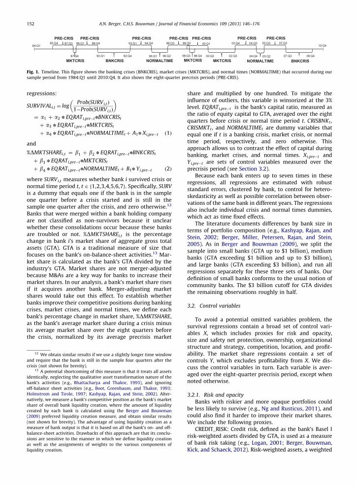
While we highlight above how we examine the effectof precrisis capital on bank performance during a crisis,we still have to address how we measure normal times. Anaıve approach would be to simply view all noncrisisquarters as such. However, if so, it is not clear then how toexamine the effect of pre-normal times capital on bankperformance during normal times. To ensure that weanalyze actual crises and normal times in a comparableway, we create ‘‘fake’’ crises to represent normal times.To construct these fake crises, we use the two longesttime periods between actual financial crises over ourentire sample period. These periods are between thecredit crunch and the Russian debt crisis, and betweenthe bursting of the dot.com bubble and the subprimelending crisis. In each case, we designate the first eightquarters between two crises as ‘‘pre-fake crisis’’ and thelast eight quarters as ‘‘post-fake crisis’’ and the remainingquarters in the middle as the fake crisis. This treatment ofthe first eight quarters as precrisis is consistent with ouranalysis of the banking and market crises. We thus end upwith a six-quarter fake crisis period between the creditcrunch and the Russian debt crisis (from 1995:Q1 to1996:Q2) and a three-quarter fake crisis period betweenthe dot.com bubble and the subprime lending crisis (from2004:Q4 to 2005:Q2).10 A timeline of the banking crises,market crises, and normal times is shown in Fig. 1.11

Our main approach pools the data to treat bankingcrises as a group, market crises as a group, and normaltimes as a group. We discuss the methodology for thisapproach here. In Section 6, we examine each crisis andnormal times individually.

Because we have two banking crises, three marketcrises, and two normal time periods (the fake crises),we have up to seven observations per bank. Usingthese data, we run the following logit survival regressionsand ordinary least squares (OLS) market share

85:Q4 87:Q3 88:Q1

87:Q4

89:Q4

90:Q1 92:Q4

93:Q1 94:Q4

95:Q1 96:Q2

96:Q3 98:Q2

98:Q3 98:Q4 00:Q2 02:Q3

02:Q4 04:Q3

04:Q4 05:Q2

05:Q3 07:Q2

07:Q3 09:Q4

00:Q184:Q1 10:Q4

PRE-CRIS PRE-CRIS PRE-CRIS PRE-CRIS PRE-CRISPRE-CRISPRE-CRIS

BNKCRISMKTCRIS NORMALTIME MKTCRIS MKTCRIS NORMALTIME BNKCRIS

Fig. 1. Timeline. This figure shows the banking crises (BNKCRIS), market crises (MKTCRIS), and normal times (NORMALTIME) that occurred during our

sample period from 1984:Q1 until 2010:Q4. It also shows the eight-quarter precrisis periods (PRE-CRIS).

A.N. Berger, C.H.S. Bouwman / Journal of Financial Economics 109 (2013) 146–176152

regressions:

SURVIVALi,t ¼ logProbðSURVi,tÞ

1�ProbðSURVi,tÞ

� �

¼ a1 þ a2 n EQRATi,pre�tnBNKCRISt

þ a3 n EQRATi,pre�tnMKTCRISt

þ a4 n EQRATi,pre�tnNORMALTIMEtþ A1n Xi,pre�t ð1Þ

and

%DMKTSHAREi,t ¼ b1 þ b2 n EQRATi,pre�tnBNKCRISt

þ b3 n EQRATi,pre�tnMKTCRISt

þ b4 n EQRATi,pre�tnNORMALTIMEtþ B1n Yi,pre�t ð2Þ

where SURVi,t measures whether bank i survived crisis ornormal time period t, t 2 f1,2,3,4,5,6,7g. Specifically, SURV

is a dummy that equals one if the bank is in the sampleone quarter before a crisis started and is still in thesample one quarter after the crisis, and zero otherwise.12

Banks that were merged within a bank holding companyare not classified as non-survivors because it unclearwhether these consolidations occur because these banksare troubled or not. %DMKTSHAREi,t is the percentagechange in bank i’s market share of aggregate gross totalassets (GTA). GTA is a traditional measure of size thatfocuses on the bank’s on-balance-sheet activities.13 Mar-ket share is calculated as the bank’s GTA divided by theindustry’s GTA. Market shares are not merger-adjustedbecause M&As are a key way for banks to increase theirmarket shares. In our analysis, a bank’s market share risesif it acquires another bank. Merger-adjusting marketshares would take out this effect. To establish whetherbanks improve their competitive positions during bankingcrises, market crises, and normal times, we define eachbank’s percentage change in market share, %DMKTSHARE,as the bank’s average market share during a crisis minusits average market share over the eight quarters beforethe crisis, normalized by its average precrisis market

12 We obtain similar results if we use a slightly longer time window

and require that the bank is still in the sample four quarters after the

crisis (not shown for brevity).13 A potential shortcoming of this measure is that it treats all assets

identically, neglecting the qualitative asset transformation nature of the

bank’s activities (e.g., Bhattacharya and Thakor, 1993), and ignoring

off-balance sheet activities (e.g., Boot, Greenbaum, and Thakor, 1993;

Holmstrom and Tirole, 1997; Kashyap, Rajan, and Stein, 2002). Alter-

natively, we measure a bank’s competitive position as the bank’s market

share of overall bank liquidity creation, where the amount of liquidity

created by each bank is calculated using the Berger and Bouwman

(2009) preferred liquidity creation measure, and obtain similar results

(not shown for brevity). The advantage of using liquidity creation as a

measure of bank output is that it is based on all the bank’s on- and off-

balance-sheet activities. Drawbacks of this approach are that its conclu-

sions are sensitive to the manner in which we define liquidity creation

as well as the assignments of weights to the various components of

liquidity creation.

share and multiplied by one hundred. To mitigate theinfluence of outliers, this variable is winsorized at the 3%level. EQRATi,pre�t is the bank’s capital ratio, measured asthe ratio of equity capital to GTA, averaged over the eightquarters before crisis or normal time period t. CRISBNKt ,CRISMKTt , and NORMALTIMEt are dummy variables thatequal one if t is a banking crisis, market crisis, or normaltime period, respectively, and zero otherwise. Thisapproach allows us to contrast the effect of capital duringbanking, market crises, and normal times. Xi,pre�t andYi,pre�t are sets of control variables measured over theprecrisis period (see Section 3.2).

Because each bank enters up to seven times in theseregressions, all regressions are estimated with robuststandard errors, clustered by bank, to control for hetero-skedasticity as well as possible correlation between obser-vations of the same bank in different years. The regressionsalso include individual crisis and normal times dummies,which act as time fixed effects.

The literature documents differences by bank size interms of portfolio composition (e.g., Kashyap, Rajan, andStein, 2002; Berger, Miller, Petersen, Rajan, and Stein,2005). As in Berger and Bouwman (2009), we split thesample into small banks (GTA up to $1 billion), mediumbanks (GTA exceeding $1 billion and up to $3 billion),and large banks (GTA exceeding $3 billion), and run allregressions separately for these three sets of banks. Ourdefinition of small banks conforms to the usual notion ofcommunity banks. The $3 billion cutoff for GTA dividesthe remaining observations roughly in half.

3.2. Control variables

To avoid a potential omitted variables problem, thesurvival regressions contain a broad set of control vari-ables X, which includes proxies for risk and opacity,size and safety net protection, ownership, organizationalstructure and strategy, competition, location, and profit-ability. The market share regressions contain a set ofcontrols Y, which excludes profitability from X. We dis-cuss the control variables in turn. Each variable is aver-aged over the eight-quarter precrisis period, except whennoted otherwise.

3.2.1. Risk and opacity

Banks with riskier and more opaque portfolios couldbe less likely to survive (e.g., Ng and Rusticus, 2011), andcould also find it harder to improve their market shares.We include the following proxies.

CREDIT_RISK: Credit risk, defined as the bank’s Basel Irisk-weighted assets divided by GTA, is used as a measureof bank risk taking (e.g., Logan, 2001; Berger, Bouwman,Kick, and Schaeck, 2012). Risk-weighted assets, a weighted

A.N. Berger, C.H.S. Bouwman / Journal of Financial Economics 109 (2013) 146–176 153

sum of the bank’s assets and off-balance-sheet activitiesdesigned to measure credit risk, is the denominator in theBasel I risk-based capital requirements. Because theserequirements became effective only in December 1990and were reported in Call Reports only from that momentonward, we use a Federal Reserve Board program toconstruct risk-weighted assets from the beginning of oursample period.

LOAN_CONCENTRATION: A bank’s loan portfolio con-centration is measured as a Herfindahl-Hirschman Index(HHI) of the following six loan categories: commercialreal estate, residential real estate, construction and indus-trial, consumer, agriculture, and other. The larger is theHHI, the more concentrated (and potentially risky) is theloan portfolio.

COMMERCIAL_REAL_ESTATE: Commercial real estatedevelopment involves long gestation periods, cyclicality,and high leverage. Cole and White (2012) find thatcommercial real estate is an important determinant ofbank failure during the recent crisis. We therefore includecommercial real estate divided by GTA.

BROKERED_DEPOSITS: Instead of attracting depositsfrom local customers, banks can obtain large depositsfrom deposit brokers. Such deposits are expensive, andthe funds are typically invested in high-risk activitiesto cover the high interest costs.14 Brokered deposits areoften used to grow quickly. Rossi (2010) suggests thatbrokered deposits do not directly explain bank failure, butFederal Deposit Insurance Corporation (2011) and Coleand White (2012) suggest otherwise. We include bro-kered deposits divided by GTA.

TRADING_ASSETS: Trading assets are assets held forresale. While these assets are transparent and liquid,trading positions are easy to change, which makes themhard to monitor. Trading has therefore been called banks’‘‘dark side’’ of liquidity (e.g., Myers and Rajan, 1998;Morgan, 2002). To capture its effect, we add trading assetsdivided by GTA to the regressions.

CASH_HOLDINGS: Cash and marketable securities arethe most liquid assets. High cash holding can reduceliquidity risk for banks and could help them survive, butthey can also be associated with agency problems (Jensen,1986). We include cash plus marketable securities dividedby GTA.

3.2.2. Size and safety net protection

SIZE: Bank size is controlled for by including the log ofGTA. In addition, we run regressions separately for small,medium, and large banks. Bank size is expected to have apositive effect on the probability of survival, because it iswell-known that larger banks have higher survival oddsthan smaller banks. In contrast, the coefficient on banksize is expected to be negative for all size classes in the

14 A statute governing brokered deposits was enacted in 1989.

According to Section 29 of the Federal Deposit Insurance Act: well

capitalized banks may accept and offer rates on brokered deposits

without restriction; adequately capitalized banks are allowed to pay

for brokered deposits up to 75 basis points over the average interest rate

paid for the deposits in the bank’s normal market area; and under-

capitalized banks are not allowed to accept brokered deposits.

market share regressions, because the law of diminishingmarginal returns suggests that it is more difficult forbigger banks (that already have larger market shares) toimprove their market shares.

CORE_DEPOSITS: Core deposits are considered to be astable source of funding. For that reason, banks that relymore on core deposits could be more likely to survive.However, as highlighted in Section 2, deposit insuranceassociated with core deposits could cause additional risktaking due to an enhanced moral hazard incentive (e.g.,Carletti, 2008; Gropp, Gruendl, and Guettler, 2010) anddue to increased competition for deposits (Matutes andVives, 1996; Hakenes and Schnabel, 2010). We thereforecalculate the amount of each bank’s core deposits usingthe Uniform Bank Performance Report (UBPR) definitionas the sum of transaction deposits, savings deposits, andsmall (denominations less than $100,000) time deposits.15

We include core deposits divided by GTA.SUPERVISOR: To capture potential differences in the

quality of oversight and leniency of supervisors, wecreate three supervisory dummies: SUPERVISOR_OCC(for national banks), SUPERVISOR_FED (for state banksthat are members of the Federal Reserve System), andSUPERVISOR_FDIC (for state nonmember banks). Weinclude only the latter two in the regressions to avoidcollinearity.

3.2.3. Ownership

BHC_MEMBER: To control for bank holding company(BHC) status, we include a dummy variable that equalsone if the bank was part of a bank holding company at anytime in the eight quarters preceding the crisis, and zerootherwise. BHC membership is expected to help a banksurvive and strengthen its competitive position becausethe holding company is required to act as a source ofstrength to all the banks it owns, and may also injectequity voluntarily when needed. Houston, James, andMarcus (1997) find that bank loan growth depends onBHC membership.

BLOCK_OWNERSHIP: Institutional block owners haveincentives to monitor management and seem to positivelyaffect the actions of firms in which they own a stake (e.g.,McConnell and Servaes, 1990; Gillan and Starks, 2000). Inbanks, however, while evidence is scarce, higher institu-tional ownership seems to be associated with greater risktaking (e.g., Mehran, Morrison, and Shapiro, 2011). Weobtain data on institutional ownership of the bank’s highestholder from the 13-F filings from Thomson Financial. Weadd up the ownership stakes of blockholders (i.e., ownershippositions of at least 5%) and assign it to each bank ownedby that high holder. Block ownership is zero for the vastmajority of banks because they are not publicly traded.

FOREIGN_OWNERSHIP: In emerging markets, foreignbanks tend to be associated with improved performanceand increased stability of the banking sector, in part becausethey reduce problems of related lending (Giannetti and

15 This definition was in place over our entire sample period. As of

March 31, 2011, the definition was revised to reflect the Federal Deposit

Insurance Corporation’s deposit insurance increase from $100,000 to

$250,000.

(footnote continued)

available on the Federal Deposit Insurance Corporation’s website based

only on the new definition. It is not possible to use the new definition for

our entire sample period.18 To illustrate, suppose there are three banks (A, B, and C) and

four markets (1, 2, 3, and 4). Suppose bank A is active in markets 1, 2,

3, and 4; B is active in 1 and 2; and C in 1. In market 1, the actual

overlap equals the overlaps of A&BþA&CþB&C¼2þ1þ1¼4, and the

maximum overlap equals (number of markets n number of banks in

the market n number of banks in the market minus 1)/2¼4n3n(3�1)/

2¼12. Market 1’s multi-market contact then equals 4/12¼0.33 (there

A.N. Berger, C.H.S. Bouwman / Journal of Financial Economics 109 (2013) 146–176154

Ongena, 2009). In contrast, Berger, DeYoung, Genay, andUdell (2000) find that foreign banks are generally lessefficient than domestic banks in the US. We thereforeinclude the percentage of foreign ownership.

3.2.4. Organizational structure and strategy

Stein (2002) argues that centralized organizations arecomplex and tend to rely on hard information, and thatdecentralized organizations are less complex and relymore on soft information. This suggests that, in additionto bank size, organizational structure and various aspectsof distance could affect performance. While we cannotmeasure the geographic distance between each bank andits customers (as do Degryse and Ongena, 2005, 2007;Bharath, Dahiya, Saunders, and Srinivasan, 2007; Degryse,Laeven, and Ongena, 2009), we can create variables thatcapture other dimensions of distance.

HQ_DEPOSITS: The fraction of deposits in a bank’s head-quarters (defined as the office with the highest amount ofdeposits) is a measure of bank centrality. Banks that aremore centralized are less complex and have shorter com-munication lines, which could affect performance.

BRANCHES / ASSETS: Banks that have more branchesper dollar of assets are more complex.

NR_STATES: Banks that are active in multiple stateshave more complex organizational structures that coverlonger distances. We include the log of the number ofstates in which the bank has branches.

3.2.5. Competition

While some theories suggest that increased competi-tion reduces franchise value and increases the likelihoodof failure (e.g., Keeley, 1990), others argue it inducesbanks to take less risk and reduces the likelihood offailure (e.g., Boyd and De Nicolo, 2005), and Martinez-Miera and Repullo (2010) suggest the relation may beU-shaped. The empirical literature also finds that compe-tition affects banks’ market shares, their ability to survive,and the stability of the banking sector (e.g., Beck,Demirguc-Kunt, and Levine, 2006; Beck, 2008).

LOCAL_MKT_POWER: We control for local marketpower by including the bank-level Herfindahl-HirschmanIndex (HHI) of deposit concentration for the local marketsin which the bank is present.16 From 1984 to 2004, wedefine the local market as the Metropolitan StatisticalArea (MSA) or non-MSA county in which the offices arelocated. After 2004, we use the new local market defini-tions based on Core Based Statistical Area (CBSA) and non-CBSA county.17 The larger is HHI, the greater is a bank’smarket power.

16 While our focus is on the change in banks’ competitive positions

measured in terms of their GTA market shares, we control for local

market power measured as the bank-level HHI based on local market

deposit shares. This is a standard measure of competition used in

antitrust analysis and research in the US. Deposits are used for this

purpose because it is the only variable for which location is known.17 When appropriate, we use New England County Metropolitan

Areas (NECMAs) instead of MSAs. CBSA collectively refers to Metropo-

litan Statistical Areas and newly-created Micropolitan Statistical Areas.

Areas based on these new standards were announced in June 2003. For

recent years, the Summary of Deposits data needed to construct HHI are

MULTI_MKT_CONTACT: Banks that operate in multiplemarkets interact with other multi-market banks in differ-ent markets. While some theories argue that multi-market contact facilitates collusion (e.g., Bernheim andWhinston, 1990), others suggest that it promotes localcompetition (e.g., Mester, 1987). To capture its effect, wefollow Evans and Kessides (1994), Degryse and Ongena(2007), and Degryse, Laeven, and Ongena (2009) andconstruct a (market-level) multi-market contact measureas the actual market overlap of all bank pairs dividedby the maximum possible overlap.18 Because our unitof observation is a bank, we calculate bank-level multi-market contact by deposit-weighting each market-levelmulti-market contact and summing over all the bank’smarkets.

3.2.6. Location

METRO_MKTS: Competition may be fiercer in metro-politan areas. The number of metropolitan markets (MSAsand CBSAs) as a fraction of all markets in which a bank isactive is therefore included in the regressions.

HOUSE_PRICE_INDEX_GROWTH: While in the mid-1980s only 20% of bank assets were exposed to realestate, by 2008 that exposure had more than doubled(Krainer, 2009). Because real estate is used as collateral,changes in real estate prices could affect bank perfor-mance. To measure its impact, we obtain two state-levelHouse Price Indices (HPIs) from the Federal HousingFinance Agency: a ‘‘purchase only’’ index (based onpurchases) and an ‘‘all transactions’’ index (based onpurchases and appraisals).19 Because bank behavior isaffected by purchases, not mere appraisals, the purchaseonly index is most appropriate for our purpose, but isavailable only from 1991 onward. For each state, wetherefore create an index using all transactions data until1990 and purchase only data from 1991 onward. For eachbank, house price index growth is then calculated as thegrowth in a state-level HPI times the fraction of the bank’sdeposits in that state, summed across all states.

are three banks in market 1 and they overlap in 1/3 of all markets).

Similarly, in market 2, the actual overlap equals the overlap of

A&B¼2, and the maximum overlap equals 3n2n(2�1)/2¼4, yielding

a multi-market contact of 2/4¼0.5 (there are two banks in market 2

and they overlap in half of all markets). In markets 3 and 4, the actual

overlap is zero because only one bank is active in each of these two

markets, and the multi-market contact therefore equals zero.19 These HPIs are based on conforming single-family properties

purchased or securitized by the Federal National Mortgage Associa-

tion (Fannie Mae) or the Federal Home Loan Mortgage Corporation

(Freddie Mac). The S&P/Case-Shiller National Home Price Index

cannot be used for our purposes because of its more limited geo-

graphic reach. It does not have valuation data from thirteen states.

20 Instead of using their proposed Stata ‘‘inteff’’ command, which

can handle only one interaction term, we used the more

flexible ‘‘margins’’ command. We thank Maarten Buis for help with

this issue.21 The regulatory environment forms another impediment: because

any bank with more than five hundred shareholders is required to

register with the Securities and Exchange Commission (SEC), many small

banks carefully maintain their shareholder base below this number

because they want to avoid the costs and hassle of registering. The JOBS

Act signed into law in April 2012 relaxes this constraint by increasing

the threshold at which small banks have to register with the SEC from

five hundred to two thousand shareholders. See Wall Street Journal

(2012).

A.N. Berger, C.H.S. Bouwman / Journal of Financial Economics 109 (2013) 146–176 155

3.2.7. Profitability

ROE: The survival regressions also include a measureof profitability because banks that are more profitablebefore the crisis could be more likely to survive crises. Weuse a bank’s return on equity (ROE), net income dividedby stockholders equity, for this purpose. ROE is a com-prehensive profitability measure, because banks mustallocate capital against every off-balance sheet activityin which they engage. Hence, net income and equity bothreflect the bank’s on- and off-balance-sheet activities. Weobtain similar results when return on assets (ROA) is usedinstead (not shown for brevity).

3.3. Sample and summary statistics

For every bank in the US, we obtain quarterly Call Reportdata from 1984:Q1 to 2010:Q4. We keep a bank-quarter inthe sample if the bank: has commercial real estate orcommercial and industrial loans outstanding; has deposits;and has gross total assets exceeding $25 million.

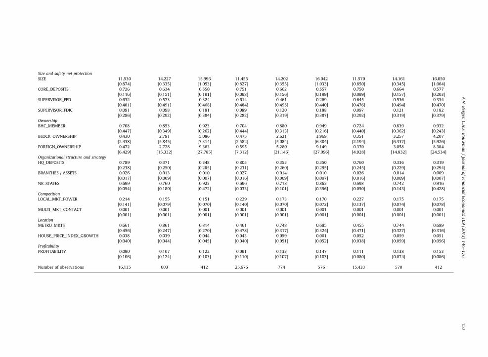
Table 1, Panel A, contains summary statistics on allregression variables for the three bank size categories(small, medium, and large) and for banking crises, marketcrises, and normal times. All financial values are put intoreal 2010:Q4 dollars [using the implicit gross domesticproduct (GDP) price deflator] before size classes are con-structed. The sample includes 57,243 small-bank, 1,946medium-bank, and 1,400 large-bank observations.

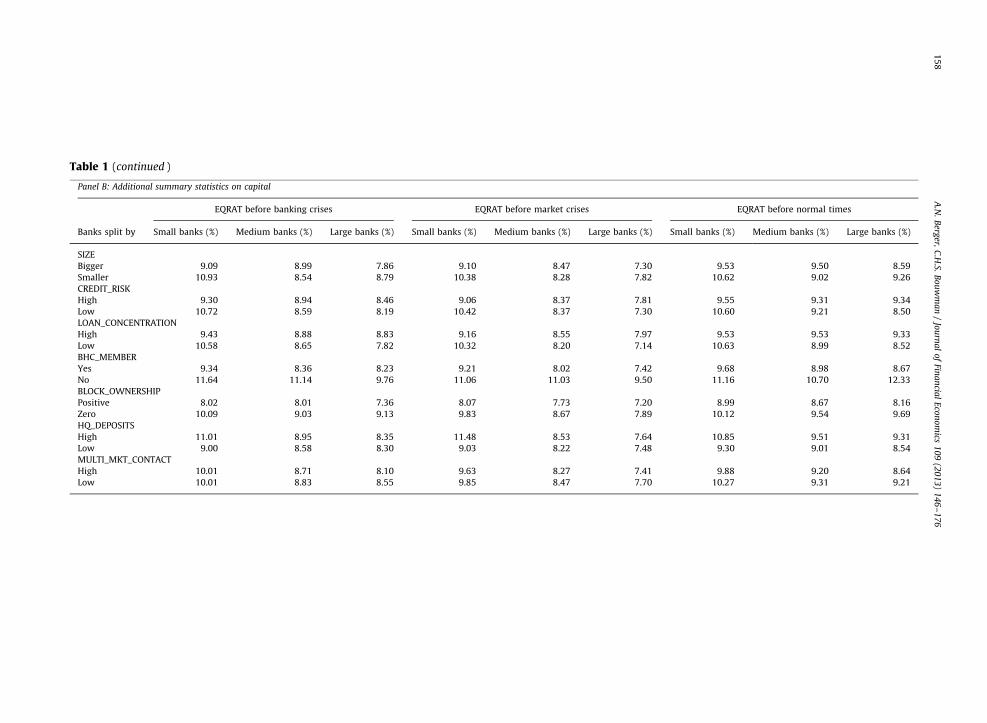
Table 1, Panel B, shows some additional summarystatistics on bank capital, our key variable of interest, toilluminate the determinants of cross-sectional heterogene-ity in capital ratios. Specifically, we take some of the keyvariables from Panel A and split banks (by size class andtime period) into two groups on the basis of the value ofthat variable to examine how capital differs across thesetwo groups. Not surprisingly, within each size class, biggerbanks (above median SIZE) operate with less capital. Whileriskier (above median CREDIT_RISK or LOAN_CONCENTRA-TION) medium and large banks hold more capital than theirless risky counterparts, this is surprisingly not true for smallbanks. Within each size class, banks that are part of a BHC(BHC_MEMBER¼yes) operate with far less capital thanthose that are not, which reflects the fact that these bankshave the option to raise additional capital from their parentif needed. Within each size class, banks with institutionalblock ownership (positive BLOCK_OWNERSHIP) and highmulti-market contact (above median MULTI_MKT_CON-TACT) operate with less capital, while those that are morecentralized (above median HQ_DEPOSITS) hold more capi-tal. While these are merely summary statistics, and identi-fying the determinants of capital is not our main goal, thesepatterns are nonetheless interesting and shed light on whybanks display nontrivial heterogeneity in capital ratios, afact that is important for understanding how differences incapital drive differences in bank performance.

4. Main regression results based on grouping bankingcrises, market crises, and normal times

In this section, we discuss the main results based ongrouping banking crises, market crises, and normal times.

We first examine the effect of capital on survival and thenanalyze its effect on market share.

4.1. Does capital affect the bank’s ability to survive during

crises and normal times?

Before presenting the survival results, it is importantto discuss a methodological issue related to the mainvariables of interest in our logit regressions being inter-action terms. In linear regressions, any interaction effectis fully captured by the coefficient on the interactionterm. This does not hold in nonlinear models as empha-sized by Norton, Wang, and Ai (2004) and Powers (2005).Strikingly, to evaluate an interaction effect in a nonlinearmodel, one cannot look at the sign, magnitude, or sig-nificance of the coefficient on the interaction term. In ourlogit model of survival, the effects of capital duringbanking crises, market crises, and normal times dependnot just on the interaction terms but also on the othercoefficients and the values of explanatory variables atwhich they are evaluated. To ensure our inferences arecorrect, we use the Norton, Wang, and Ai (2004) metho-dology to calculate the correct marginal effects andt-statistics.20

Table 2 presents the survival findings for small, med-ium, and large banks. Panel A contains the regressionparameters. The coefficients on the capital–crisis interac-tion terms should be ignored in this panel. Panel B showsthe marginal effects of the main variables of interest.

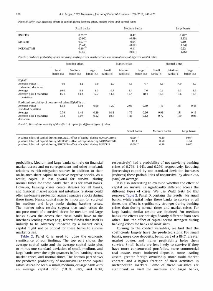
Two main results are apparent. First, higher capitalhelps small banks to improve their odds of survival atall times (during banking crises, market crises,and normal times). Second, higher capital helps mediumand large banks improve the probability of survivingbanking crises (significant for large banks). These resultsgenerally support the hypothesis that capital helps bankssurvive.

These findings have sensible economic interpretations.Capital is the main line of defense against negative shocks.For small banks, capital is important at all times, becausethey face shocks more often than medium and large banks,and they have limited (and relatively costly) access to thefinancial market in the event of unanticipated needs.21

In fact, the number of small banks has been dwindlingsince the mid-1980s. Hence, higher capital enhances theprobability of survival for such banks at all times. Thisfinding is consistent with the theoretical papers thatpredict that higher capital increases a bank’s survival

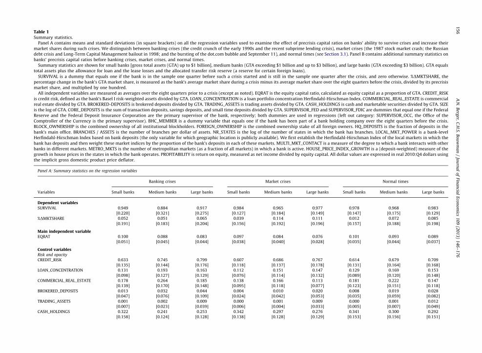
Table 1Summary statistics.

Panel A contains means and standard deviations (in square brackets) on all the regression variables used to examine the effect of precrisis capital ratios on banks’ ability to survive crises and increase their

market shares during such crises. We distinguish between banking crises (the credit crunch of the early 1990s and the recent subprime lending crisis), market crises (the 1987 stock market crash; the Russian

debt crisis and Long-Term Capital Management bailout in 1998; and the bursting of the dot.com bubble and September 11), and normal times (see Section 3.1). Panel B contains additional summary statistics on

banks’ precrisis capital ratios before banking crises, market crises, and normal times.

Summary statistics are shown for small banks [gross total assets (GTA) up to $1 billion], medium banks (GTA exceeding $1 billion and up to $3 billion), and large banks (GTA exceeding $3 billion). GTA equals

total assets plus the allowance for loan and the lease losses and the allocated transfer risk reserve (a reserve for certain foreign loans).

SURVIVAL is a dummy that equals one if the bank is in the sample one quarter before such a crisis started and is still in the sample one quarter after the crisis, and zero otherwise. %DMKTSHARE, the

percentage change in the bank’s GTA market share, is measured as the bank’s average market share during a crisis minus its average market share over the eight quarters before the crisis, divided by its precrisis

market share, and multiplied by one hundred.

All independent variables are measured as averages over the eight quarters prior to a crisis (except as noted). EQRAT is the equity capital ratio, calculated as equity capital as a proportion of GTA. CREDIT_RISK

is credit risk, defined as the bank’s Basel I risk-weighted assets divided by GTA. LOAN_CONCENTRATION is a loan portfolio concentration Herfindahl-Hirschman Index. COMMERCIAL_REAL_ESTATE is commercial

real estate divided by GTA. BROKERED-DEPOSITS is brokered deposits divided by GTA. TRADING_ASSETS is trading assets divided by GTA. CASH_HOLDINGS is cash and marketable securities divided by GTA. SIZE

is the log of GTA. CORE_DEPOSITS is the sum of transaction deposits, savings deposits, and small time deposits divided by GTA. SUPERVISOR_FED and SUPERVISOR_FDIC are dummies that equal one if the Federal

Reserve and the Federal Deposit Insurance Corporation are the primary supervisor of the bank, respectively; both dummies are used in regressions (left out category: SUPERVISOR_OCC, the Office of the

Comptroller of the Currency is the primary supervisor). BHC_MEMBER is a dummy variable that equals one if the bank has been part of a bank holding company over the eight quarters before the crisis.

BLOCK_OWNERSHIP is the combined ownership of all institutional blockholders. FOREIGN_OWNERSHIP is the combined ownership stake of all foreign owners. HQ_DEPOSITS is the fraction of deposits in the

bank’s main office. BRANCHES / ASSETS is the number of branches per dollar of assets. NR_STATES is the log of the number of states in which the bank has branches. LOCAL_MKT_POWER is a bank-level

Herfindahl-Hirschman Index based on bank deposits (the only variable for which geographic location is publicly available). We first establish the Herfindahl-Hirschman Index of the local markets in which the

bank has deposits and then weight these market indices by the proportion of the bank’s deposits in each of these markets. MULTI_MKT_CONTACT is a measure of the degree to which a bank interacts with other

banks in different markets. METRO_MKTS is the number of metropolitan markets (as a fraction of all markets) in which a bank is active. HOUSE_PRICE_INDEX_GROWTH is a (deposit-weighted) measure of the

growth in house prices in the states in which the bank operates. PROFITABILITY is return on equity, measured as net income divided by equity capital. All dollar values are expressed in real 2010:Q4 dollars using

the implicit gross domestic product price deflator.

Panel A: Summary statistics on the regression variables

Banking crises Market crises Normal times

Variables Small banks Medium banks Large banks Small banks Medium banks Large banks Small banks Medium banks Large banks

Dependent variablesSURVIVAL 0.949 0.884 0.917 0.984 0.965 0.977 0.978 0.968 0.983

[0.220] [0.321] [0.275] [0.127] [0.184] [0.149] [0.147] [0.175] [0.129]

%DMKTSHARE 0.052 0.051 0.065 0.039 0.114 0.111 0.012 0.072 0.085

[0.191] [0.183] [0.204] [0.156] [0.192] [0.196] [0.157] [0.188] [0.198]

Main independent variableEQRAT 0.100 0.088 0.083 0.097 0.084 0.076 0.101 0.093 0.089

[0.051] [0.045] [0.044] [0.038] [0.040] [0.028] [0.035] [0.044] [0.037]

Control variablesRisk and opacity

CREDIT_RISK 0.633 0.745 0.799 0.607 0.686 0.767 0.614 0.679 0.709

[0.135] [0.144] [0.176] [0.118] [0.137] [0.178] [0.131] [0.164] [0.168]

LOAN_CONCENTRATION 0.131 0.193 0.163 0.112 0.151 0.147 0.129 0.169 0.153

[0.098] [0.127] [0.129] [0.076] [0.114] [0.132] [0.089] [0.120] [0.148]

COMMERCIAL_REAL_ESTATE 0.178 0.264 0.185 0.138 0.166 0.113 0.181 0.222 0.147

[0.139] [0.170] [0.148] [0.095] [0.118] [0.077] [0.123] [0.151] [0.118]

BROKERED_DEPOSITS 0.013 0.032 0.044 0.004 0.010 0.020 0.008 0.019 0.028

[0.047] [0.076] [0.109] [0.024] [0.042] [0.053] [0.035] [0.059] [0.082]

TRADING_ASSETS 0.001 0.002 0.009 0.000 0.001 0.009 0.000 0.001 0.012

[0.007] [0.023] [0.039] [0.006] [0.004] [0.033] [0.005] [0.007] [0.049]

CASH_HOLDINGS 0.322 0.241 0.253 0.342 0.297 0.276 0.341 0.300 0.292

[0.158] [0.124] [0.128] [0.138] [0.128] [0.129] [0.153] [0.156] [0.151]

A.N

.B

erger,

C.H

.S.B

ou

wm

an

/Jo

urn

al

of

Fina

ncia

lE

con

om

ics1

09

(20

13

)1

46

–1

76

15

6

Size and safety net protection

SIZE 11.530 14.227 15.996 11.455 14.202 16.042 11.570 14.161 16.050

[0.874] [0.335] [1.053] [0.827] [0.355] [1.033] [0.850] [0.345] [1.064]

CORE_DEPOSITS 0.726 0.634 0.550 0.751 0.662 0.557 0.750 0.664 0.577

[0.116] [0.151] [0.191] [0.098] [0.156] [0.199] [0.099] [0.157] [0.203]

SUPERVISOR_FED 0.632 0.573 0.324 0.614 0.461 0.269 0.645 0.536 0.334

[0.481] [0.491] [0.468] [0.484] [0.495] [0.440] [0.476] [0.494] [0.470]

SUPERVISOR_FDIC 0.091 0.098 0.181 0.089 0.120 0.188 0.097 0.121 0.182

[0.286] [0.292] [0.384] [0.282] [0.319] [0.387] [0.292] [0.319] [0.379]

Ownership

BHC_MEMBER 0.708 0.853 0.923 0.704 0.880 0.949 0.724 0.839 0.932

[0.447] [0.349] [0.262] [0.444] [0.313] [0.216] [0.440] [0.362] [0.243]

BLOCK_OWNERSHIP 0.430 2.781 5.086 0.475 2.621 3.969 0.351 3.257 4.207

[2.438] [5.845] [7.314] [2.582] [5.084] [6.304] [2.194] [6.337] [5.926]

FOREIGN_OWNERSHIP 0.472 2.728 9.363 0.595 5.280 9.149 0.370 3.058 8.384

[6.429] [15.332] [27.785] [7.312] [21.146] [27.096] [4.928] [14.832] [24.534]

Organizational structure and strategy

HQ_DEPOSITS 0.789 0.371 0.348 0.805 0.353 0.350 0.760 0.336 0.319

[0.238] [0.250] [0.285] [0.231] [0.260] [0.295] [0.245] [0.229] [0.294]

BRANCHES / ASSETS 0.026 0.013 0.010 0.027 0.014 0.010 0.026 0.014 0.009

[0.017] [0.009] [0.007] [0.016] [0.009] [0.007] [0.016] [0.009] [0.007]

NR_STATES 0.699 0.760 0.923 0.696 0.718 0.863 0.698 0.742 0.916

[0.054] [0.180] [0.472] [0.033] [0.101] [0.356] [0.050] [0.143] [0.428]

Competition

LOCAL_MKT_POWER 0.214 0.155 0.151 0.229 0.173 0.170 0.227 0.175 0.175

[0.141] [0.079] [0.070] [0.140] [0.070] [0.072] [0.137] [0.074] [0.078]

MULTI_MKT_CONTACT 0.001 0.001 0.001 0.001 0.001 0.001 0.001 0.001 0.001

[0.001] [0.001] [0.001] [0.001] [0.001] [0.001] [0.001] [0.001] [0.001]

Location

METRO_MKTS 0.661 0.861 0.814 0.461 0.748 0.685 0.455 0.744 0.689

[0.456] [0.247] [0.270] [0.478] [0.317] [0.324] [0.471] [0.327] [0.316]

HOUSE_PRICE_INDEX_GROWTH 0.038 0.039 0.044 0.043 0.059 0.061 0.052 0.059 0.051

[0.040] [0.044] [0.045] [0.040] [0.051] [0.052] [0.038] [0.059] [0.056]

Profitability

PROFITABILITY 0.090 0.107 0.122 0.091 0.133 0.147 0.111 0.138 0.153

[0.106] [0.124] [0.103] [0.110] [0.107] [0.103] [0.080] [0.074] [0.086]

Number of observations 16,135 603 412 25,676 774 576 15,433 570 412

A.N

.B

erger,

C.H

.S.B

ou

wm

an

/Jo

urn

al

of

Fina

ncia

lE

con

om

ics1

09

(20

13

)1

46

–1

76

15

7

Panel B: Additional summary statistics on capital

EQRAT before banking crises EQRAT before market crises EQRAT before normal times

Banks split by Small banks (%) Medium banks (%) Large banks (%) Small banks (%) Medium banks (%) Large banks (%) Small banks (%) Medium banks (%) Large banks (%)

SIZE

Bigger 9.09 8.99 7.86 9.10 8.47 7.30 9.53 9.50 8.59

Smaller 10.93 8.54 8.79 10.38 8.28 7.82 10.62 9.02 9.26

CREDIT_RISK

High 9.30 8.94 8.46 9.06 8.37 7.81 9.55 9.31 9.34

Low 10.72 8.59 8.19 10.42 8.37 7.30 10.60 9.21 8.50

LOAN_CONCENTRATION

High 9.43 8.88 8.83 9.16 8.55 7.97 9.53 9.53 9.33

Low 10.58 8.65 7.82 10.32 8.20 7.14 10.63 8.99 8.52

BHC_MEMBER

Yes 9.34 8.36 8.23 9.21 8.02 7.42 9.68 8.98 8.67

No 11.64 11.14 9.76 11.06 11.03 9.50 11.16 10.70 12.33

BLOCK_OWNERSHIP

Positive 8.02 8.01 7.36 8.07 7.73 7.20 8.99 8.67 8.16

Zero 10.09 9.03 9.13 9.83 8.67 7.89 10.12 9.54 9.69

HQ_DEPOSITS

High 11.01 8.95 8.35 11.48 8.53 7.64 10.85 9.51 9.31

Low 9.00 8.58 8.30 9.03 8.22 7.48 9.30 9.01 8.54

MULTI_MKT_CONTACT

High 10.01 8.71 8.10 9.63 8.27 7.41 9.88 9.20 8.64

Low 10.01 8.83 8.55 9.85 8.47 7.70 10.27 9.31 9.21

Table 1 (continued )

A.N

.B

erger,

C.H

.S.B

ou

wm

an

/Jo

urn

al

of

Fina

ncia

lE

con

om

ics1

09

(20

13

)1

46

–1

76

15

8

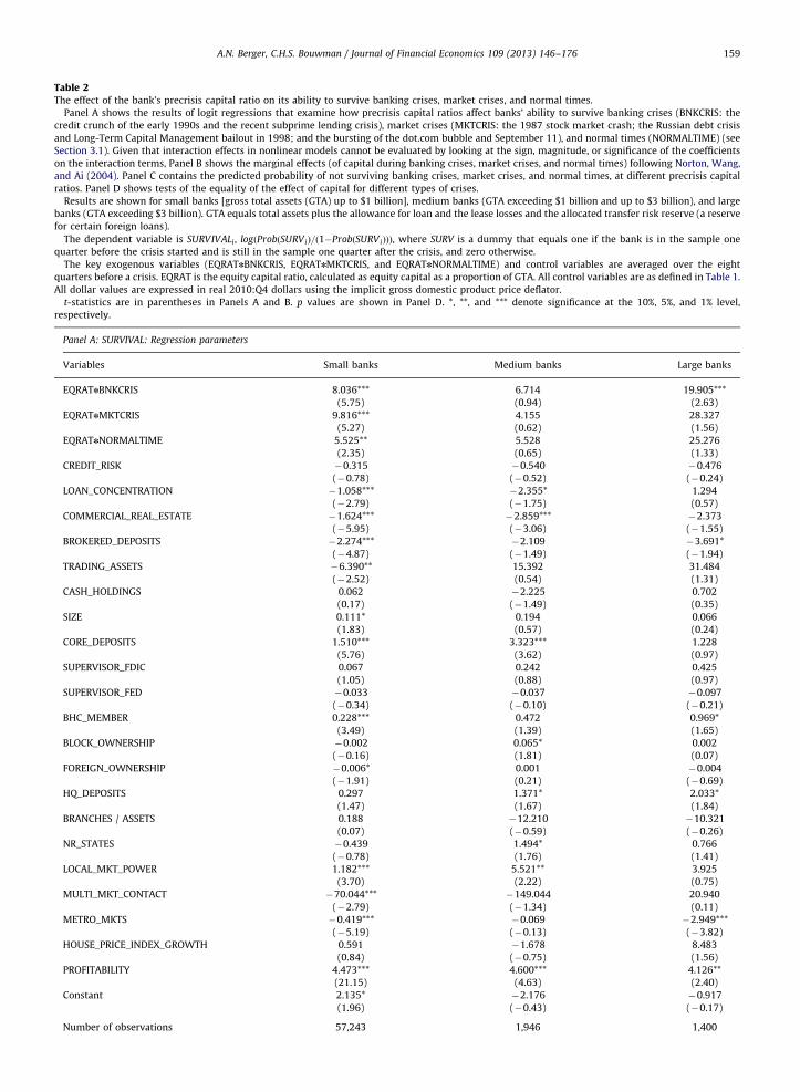
Table 2The effect of the bank’s precrisis capital ratio on its ability to survive banking crises, market crises, and normal times.

Panel A shows the results of logit regressions that examine how precrisis capital ratios affect banks’ ability to survive banking crises (BNKCRIS: the

credit crunch of the early 1990s and the recent subprime lending crisis), market crises (MKTCRIS: the 1987 stock market crash; the Russian debt crisis

and Long-Term Capital Management bailout in 1998; and the bursting of the dot.com bubble and September 11), and normal times (NORMALTIME) (see

Section 3.1). Given that interaction effects in nonlinear models cannot be evaluated by looking at the sign, magnitude, or significance of the coefficients

on the interaction terms, Panel B shows the marginal effects (of capital during banking crises, market crises, and normal times) following Norton, Wang,

and Ai (2004). Panel C contains the predicted probability of not surviving banking crises, market crises, and normal times, at different precrisis capital

ratios. Panel D shows tests of the equality of the effect of capital for different types of crises.

Results are shown for small banks [gross total assets (GTA) up to $1 billion], medium banks (GTA exceeding $1 billion and up to $3 billion), and large

banks (GTA exceeding $3 billion). GTA equals total assets plus the allowance for loan and the lease losses and the allocated transfer risk reserve (a reserve

for certain foreign loans).

The dependent variable is SURVIVALi , logðProbðSURViÞ=ð1�ProbðSURViÞÞÞ, where SURV is a dummy that equals one if the bank is in the sample one

quarter before the crisis started and is still in the sample one quarter after the crisis, and zero otherwise.

The key exogenous variables (EQRATnBNKCRIS, EQRATnMKTCRIS, and EQRATnNORMALTIME) and control variables are averaged over the eight

quarters before a crisis. EQRAT is the equity capital ratio, calculated as equity capital as a proportion of GTA. All control variables are as defined in Table 1.

All dollar values are expressed in real 2010:Q4 dollars using the implicit gross domestic product price deflator.

t-statistics are in parentheses in Panels A and B. p values are shown in Panel D. *, **, and *** denote significance at the 10%, 5%, and 1% level,

respectively.

Panel A: SURVIVAL: Regression parameters

Variables Small banks Medium banks Large banks

EQRATnBNKCRIS 8.036*** 6.714 19.905***

(5.75) (0.94) (2.63)

EQRATnMKTCRIS 9.816*** 4.155 28.327

(5.27) (0.62) (1.56)

EQRATnNORMALTIME 5.525** 5.528 25.276

(2.35) (0.65) (1.33)

CREDIT_RISK �0.315 �0.540 �0.476

(�0.78) (�0.52) (�0.24)

LOAN_CONCENTRATION �1.058*** �2.355* 1.294

(�2.79) (�1.75) (0.57)

COMMERCIAL_REAL_ESTATE �1.624*** �2.859*** �2.373

(�5.95) (�3.06) (�1.55)

BROKERED_DEPOSITS �2.274*** �2.109 �3.691*

(�4.87) (�1.49) (�1.94)

TRADING_ASSETS �6.390** 15.392 31.484

(�2.52) (0.54) (1.31)

CASH_HOLDINGS 0.062 �2.225 0.702

(0.17) (�1.49) (0.35)

SIZE 0.111* 0.194 0.066

(1.83) (0.57) (0.24)

CORE_DEPOSITS 1.510*** 3.323*** 1.228

(5.76) (3.62) (0.97)

SUPERVISOR_FDIC 0.067 0.242 0.425

(1.05) (0.88) (0.97)

SUPERVISOR_FED �0.033 �0.037 �0.097

(�0.34) (�0.10) (�0.21)

BHC_MEMBER 0.228*** 0.472 0.969*

(3.49) (1.39) (1.65)

BLOCK_OWNERSHIP �0.002 0.065* 0.002

(�0.16) (1.81) (0.07)

FOREIGN_OWNERSHIP �0.006* 0.001 �0.004

(�1.91) (0.21) (�0.69)

HQ_DEPOSITS 0.297 1.371* 2.033*

(1.47) (1.67) (1.84)

BRANCHES / ASSETS 0.188 �12.210 �10.321

(0.07) (�0.59) (�0.26)

NR_STATES �0.439 1.494* 0.766

(�0.78) (1.76) (1.41)

LOCAL_MKT_POWER 1.182*** 5.521** 3.925

(3.70) (2.22) (0.75)

MULTI_MKT_CONTACT �70.044*** �149.044 20.940

(�2.79) (�1.34) (0.11)

METRO_MKTS �0.419*** �0.069 �2.949***

(�5.19) (�0.13) (�3.82)

HOUSE_PRICE_INDEX_GROWTH 0.591 �1.678 8.483

(0.84) (�0.75) (1.56)

PROFITABILITY 4.473*** 4.600*** 4.126**

(21.15) (4.63) (2.40)

Constant 2.135* �2.176 �0.917

(1.96) (�0.43) (�0.17)

Number of observations 57,243 1,946 1,400

A.N. Berger, C.H.S. Bouwman / Journal of Financial Economics 109 (2013) 146–176 159

Panel B: SURVIVAL: Marginal effects of capital during banking crises, market crises, and normal times

Small banks Medium banks Large banks

BNKCRIS 0.29*** 0.47 0.70**

(5.96) (0.99) (2.32)

MKTCRIS 0.07*** 0.04 0.10

(5.41) (0.62) (1.34)

NORMALTIME 0.10*** 0.11 0.22

(3.55) (0.91) (1.36)

Panel C: Predicted probability of not surviving banking crises, market crises, and normal times at different capital ratios

Banking crises Market crises Normal times

Small

banks (%)

Medium

banks (%)

Large

banks (%)

Small

banks (%)

Medium

banks (%)

Large

banks (%)

Small

banks (%)

Medium

banks (%)

Large

banks (%)

EQRAT:

Average minus 1

standard deviation

4.9 4.3 3.9 5.9 4.3 4.7 6.6 4.9 5.2

Average 10.0 8.8 8.3 9.7 8.4 7.6 10.1 9.3 8.9

Average plus 1 standard

deviation

15.1 13.2 12.7 13.5 12.4 10.4 13.6 13.6 12.6

Predicted probability of nonsurvival when EQRAT is at:

Average minus 1

standard deviation

1.18 1.94 0.69 1.20 2.06 0.59 1.13 1.91 0.48

Average 0.79 1.44 0.29 0.83 1.75 0.26 0.93 1.51 0.19

Average plus 1 standard

deviation

0.52 1.07 0.12 0.57 1.48 0.12 0.77 1.19 0.08

Panel D: Tests of the equality of the effect of capital for different types of crises

Small banks Medium banks Large banks

p value: Effect of capital during BNKCRIS¼effect of capital during NORMALTIME 0.00*** 0.39 0.07*

p value: Effect of capital during MKTCRIS¼effect of capital during NORMALTIME 0.14 0.50 0.34

p value: Effect of capital during BNKCRIS¼effect of capital during MKTCRIS 0.00*** 0.38 0.06*

A.N. Berger, C.H.S. Bouwman / Journal of Financial Economics 109 (2013) 146–176160

probability. Medium and large banks can rely on financialmarket access and on correspondent and other interbankrelations as risk-mitigation sources in addition to theiron-balance-sheet capital to survive negative shocks. As aresult, capital is less pivotal for survival duringnormal times for these banks than it is for small banks.However, banking crises create stresses for all banks,and financial market access and interbank relations couldoffer inadequate protection against negative shocks duringthese times. Hence, capital may be important for survivalfor medium and large banks during banking crises.The market crisis results suggest that such crises donot pose much of a survival threat for medium and largebanks. Given the access that these banks have to theinterbank lending market (e.g., federal funds) that itself isunlikely to be adversely impacted by a market crisis,capital might not be critical for these banks to survivemarket crises.

Table 2, Panel C, is used to judge the economicsignificance of our findings. The top part shows theaverage capital ratio and the average capital ratio plusor minus one standard deviation of small, medium, andlarge banks over the eight quarters before banking crises,market crises, and normal times. The bottom part showsthe predicted probability of nonsurvival at these capitalratios. As can be seen, a small, medium, or large bank withan average capital ratio (10.0%, 8.8%, and 8.3%,

respectively) had a probability of not surviving bankingcrises of 0.79%, 1.44%, and 0.29%, respectively. Reducing(increasing) capital by one standard deviation increases(reduces) these probabilities of nonsurvival by about 75%(50%) on average.

It is also interesting to examine whether the effect ofcapital on survival is significantly different across thedifferent types of crises. We use Wald tests for thispurpose. Table 2, Panel D, contains the results. For smallbanks, while capital helps these banks to survive at alltimes, the effect is significantly stronger during bankingcrises than during normal times and market crises. Forlarge banks, similar results are obtained. For mediumbanks, the effects are not significantly different from eachother. Thus, the effect of capital seems strongest duringbanking crises for banks of most sizes.

Turning to the control variables, we find that thecoefficients largely have the predicted signs. For smallbanks, more core deposits, being part of a BHC, greatermarket power, and higher profitability helps themsurvive. Small banks are less likely to survive if theyhave more concentrated portfolios, more commercialreal estate, more brokered deposits, more tradingassets, greater foreign ownership, more multi-marketcontact, and a higher fraction of their activities inmetropolitan markets. Some of these variables aresignificant as well for medium and large banks,

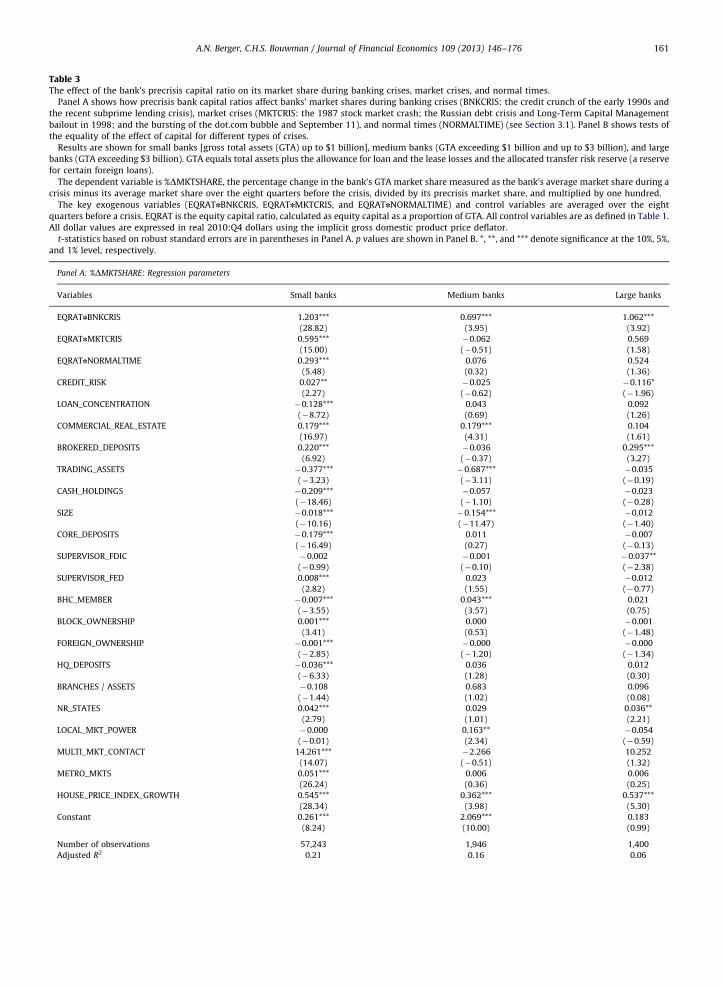
Table 3The effect of the bank’s precrisis capital ratio on its market share during banking crises, market crises, and normal times.

Panel A shows how precrisis bank capital ratios affect banks’ market shares during banking crises (BNKCRIS: the credit crunch of the early 1990s and

the recent subprime lending crisis), market crises (MKTCRIS: the 1987 stock market crash; the Russian debt crisis and Long-Term Capital Management

bailout in 1998; and the bursting of the dot.com bubble and September 11), and normal times (NORMALTIME) (see Section 3.1). Panel B shows tests of

the equality of the effect of capital for different types of crises.

Results are shown for small banks [gross total assets (GTA) up to $1 billion], medium banks (GTA exceeding $1 billion and up to $3 billion), and large

banks (GTA exceeding $3 billion). GTA equals total assets plus the allowance for loan and the lease losses and the allocated transfer risk reserve (a reserve

for certain foreign loans).

The dependent variable is %DMKTSHARE, the percentage change in the bank’s GTA market share measured as the bank’s average market share during a

crisis minus its average market share over the eight quarters before the crisis, divided by its precrisis market share, and multiplied by one hundred.

The key exogenous variables (EQRATnBNKCRIS, EQRATnMKTCRIS, and EQRATnNORMALTIME) and control variables are averaged over the eight

quarters before a crisis. EQRAT is the equity capital ratio, calculated as equity capital as a proportion of GTA. All control variables are as defined in Table 1.

All dollar values are expressed in real 2010:Q4 dollars using the implicit gross domestic product price deflator.

t-statistics based on robust standard errors are in parentheses in Panel A. p values are shown in Panel B. *, **, and *** denote significance at the 10%, 5%,

and 1% level, respectively.

Panel A: %DMKTSHARE: Regression parameters

Variables Small banks Medium banks Large banks

EQRATnBNKCRIS 1.203*** 0.697*** 1.062***

(28.82) (3.95) (3.92)

EQRATnMKTCRIS 0.595*** �0.062 0.569

(15.00) (�0.51) (1.58)

EQRATnNORMALTIME 0.293*** 0.076 0.524

(5.48) (0.32) (1.36)

CREDIT_RISK 0.027** �0.025 �0.116*

(2.27) (�0.62) (�1.96)

LOAN_CONCENTRATION �0.128*** 0.043 0.092

(�8.72) (0.69) (1.26)

COMMERCIAL_REAL_ESTATE 0.179*** 0.179*** 0.104

(16.97) (4.31) (1.61)

BROKERED_DEPOSITS 0.220*** �0.036 0.295***

(6.92) (�0.37) (3.27)

TRADING_ASSETS �0.377*** �0.687*** �0.035

(�3.23) (�3.11) (�0.19)

CASH_HOLDINGS �0.209*** �0.057 �0.023

(�18.46) (�1.10) (�0.28)

SIZE �0.018*** �0.154*** �0.012

(�10.16) (�11.47) (�1.40)

CORE_DEPOSITS �0.179*** 0.011 �0.007

(�16.49) (0.27) (�0.13)

SUPERVISOR_FDIC �0.002 �0.001 �0.037**

(�0.99) (�0.10) (�2.38)

SUPERVISOR_FED 0.008*** 0.023 �0.012

(2.82) (1.55) (�0.77)

BHC_MEMBER �0.007*** 0.043*** 0.021

(�3.55) (3.57) (0.75)

BLOCK_OWNERSHIP 0.001*** 0.000 �0.001

(3.41) (0.53) (�1.48)

FOREIGN_OWNERSHIP �0.001*** �0.000 �0.000

(�2.85) (�1.20) (�1.34)

HQ_DEPOSITS �0.036*** 0.036 0.012

(�6.33) (1.28) (0.30)

BRANCHES / ASSETS �0.108 0.683 0.096

(�1.44) (1.02) (0.08)

NR_STATES 0.042*** 0.029 0.036**

(2.79) (1.01) (2.21)

LOCAL_MKT_POWER �0.000 0.163** �0.054

(�0.01) (2.34) (�0.59)

MULTI_MKT_CONTACT 14.261*** �2.266 10.252

(14.07) (�0.51) (1.32)

METRO_MKTS 0.051*** 0.006 0.006

(26.24) (0.36) (0.25)

HOUSE_PRICE_INDEX_GROWTH 0.545*** 0.362*** 0.537***

(28.34) (3.98) (5.30)

Constant 0.261*** 2.069*** 0.183

(8.24) (10.00) (0.99)

Number of observations 57,243 1,946 1,400

Adjusted R2 0.21 0.16 0.06

A.N. Berger, C.H.S. Bouwman / Journal of Financial Economics 109 (2013) 146–176 161

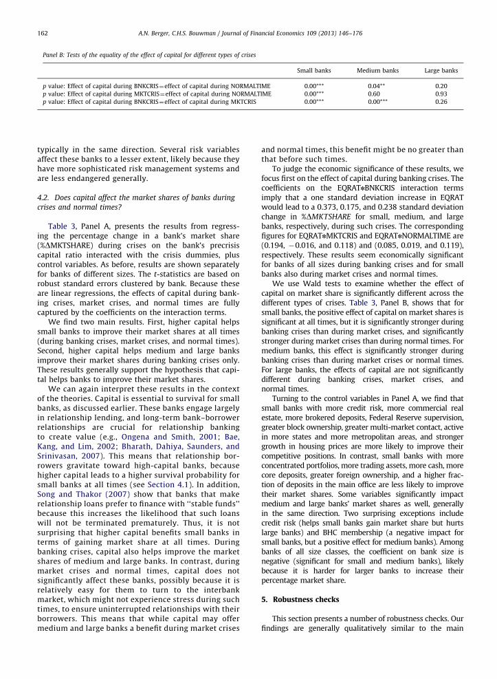
Panel B: Tests of the equality of the effect of capital for different types of crises

Small banks Medium banks Large banks

p value: Effect of capital during BNKCRIS¼effect of capital during NORMALTIME 0.00*** 0.04** 0.20

p value: Effect of capital during MKTCRIS¼effect of capital during NORMALTIME 0.00*** 0.60 0.93

p value: Effect of capital during BNKCRIS¼effect of capital during MKTCRIS 0.00*** 0.00*** 0.26

A.N. Berger, C.H.S. Bouwman / Journal of Financial Economics 109 (2013) 146–176162

typically in the same direction. Several risk variablesaffect these banks to a lesser extent, likely because theyhave more sophisticated risk management systems andare less endangered generally.

4.2. Does capital affect the market shares of banks during

crises and normal times?

Table 3, Panel A, presents the results from regress-ing the percentage change in a bank’s market share(%DMKTSHARE) during crises on the bank’s precrisiscapital ratio interacted with the crisis dummies, pluscontrol variables. As before, results are shown separatelyfor banks of different sizes. The t-statistics are based onrobust standard errors clustered by bank. Because theseare linear regressions, the effects of capital during bank-ing crises, market crises, and normal times are fullycaptured by the coefficients on the interaction terms.

We find two main results. First, higher capital helpssmall banks to improve their market shares at all times(during banking crises, market crises, and normal times).Second, higher capital helps medium and large banksimprove their market shares during banking crises only.These results generally support the hypothesis that capi-tal helps banks to improve their market shares.

We can again interpret these results in the contextof the theories. Capital is essential to survival for smallbanks, as discussed earlier. These banks engage largelyin relationship lending, and long-term bank–borrowerrelationships are crucial for relationship bankingto create value (e.g., Ongena and Smith, 2001; Bae,Kang, and Lim, 2002; Bharath, Dahiya, Saunders, andSrinivasan, 2007). This means that relationship bor-rowers gravitate toward high-capital banks, becausehigher capital leads to a higher survival probability forsmall banks at all times (see Section 4.1). In addition,Song and Thakor (2007) show that banks that makerelationship loans prefer to finance with ‘‘stable funds’’because this increases the likelihood that such loanswill not be terminated prematurely. Thus, it is notsurprising that higher capital benefits small banks interms of gaining market share at all times. Duringbanking crises, capital also helps improve the marketshares of medium and large banks. In contrast, duringmarket crises and normal times, capital does notsignificantly affect these banks, possibly because it isrelatively easy for them to turn to the interbankmarket, which might not experience stress during suchtimes, to ensure uninterrupted relationships with theirborrowers. This means that while capital may offermedium and large banks a benefit during market crises

and normal times, this benefit might be no greater thanthat before such times.

To judge the economic significance of these results, wefocus first on the effect of capital during banking crises. Thecoefficients on the EQRATnBNKCRIS interaction termsimply that a one standard deviation increase in EQRATwould lead to a 0.373, 0.175, and 0.238 standard deviationchange in %DMKTSHARE for small, medium, and largebanks, respectively, during such crises. The correspondingfigures for EQRATnMKTCRIS and EQRATnNORMALTIME are(0.194, �0.016, and 0.118) and (0.085, 0.019, and 0.119),respectively. These results seem economically significantfor banks of all sizes during banking crises and for smallbanks also during market crises and normal times.

We use Wald tests to examine whether the effect ofcapital on market share is significantly different across thedifferent types of crises. Table 3, Panel B, shows that forsmall banks, the positive effect of capital on market shares issignificant at all times, but it is significantly stronger duringbanking crises than during market crises, and significantlystronger during market crises than during normal times. Formedium banks, this effect is significantly stronger duringbanking crises than during market crises or normal times.For large banks, the effects of capital are not significantlydifferent during banking crises, market crises, andnormal times.

Turning to the control variables in Panel A, we find thatsmall banks with more credit risk, more commercial realestate, more brokered deposits, Federal Reserve supervision,greater block ownership, greater multi-market contact, activein more states and more metropolitan areas, and strongergrowth in housing prices are more likely to improve theircompetitive positions. In contrast, small banks with moreconcentrated portfolios, more trading assets, more cash, morecore deposits, greater foreign ownership, and a higher frac-tion of deposits in the main office are less likely to improvetheir market shares. Some variables significantly impactmedium and large banks’ market shares as well, generallyin the same direction. Two surprising exceptions includecredit risk (helps small banks gain market share but hurtslarge banks) and BHC membership (a negative impact forsmall banks, but a positive effect for medium banks). Amongbanks of all size classes, the coefficient on bank size isnegative (significant for small and medium banks), likelybecause it is harder for larger banks to increase theirpercentage market share.

5. Robustness checks

This section presents a number of robustness checks. Ourfindings are generally qualitatively similar to the main

A.N. Berger, C.H.S. Bouwman / Journal of Financial Economics 109 (2013) 146–176 163

results. The same control variables as used in the mainregressions are included with some exceptions noted below.To preserve space, we present only the results of interest.Our (nonlinear) survival regressions show marginal effectsto ensure correct inference (see Section 4.1) during bankingcrises, market crises, and normal times, while our (linear)market share regressions show the coefficients on thecapital–crisis interaction terms.

5.1. Use regulatory capital ratios

One may wonder to what extent the main results arespecific to our choice of the definition of capital, EQRAT,the ratio of equity capital to assets. To examine this issue,we rerun our regressions using regulatory capital ratios.Basel I introduced two risk-based capital ratios, the Tier 1and Total risk-based capital ratios. Because these ratiosbecame fully effective only as of December 1990, we useeach bank’s ratio of equity capital to GTA before this dateand its Tier 1 risk-based capital ratio from that momentonward. We obtain similar results when we use the Totalrisk-based capital ratio instead of the Tier 1 capital ratio.22

Table 4, Panel A, shows the results. They are broadlysimilar to the main results (see Tables 2 and 3) except thatfor small banks, we find no effect on survival during normaltimes; for medium banks, the effect of capital on survivalbecomes significant during banking crises while the effect onmarket share loses significance (t-statistic 1.62); for largebanks, capital now helps survival during normal timesas well.

We also run all the robustness checks presented in therest of this section using regulatory capital and obtainresults that are similar to the main results (not shown forbrevity). Nonetheless, we believe that our choice of usingEQRAT in the main regressions is appropriate. The reg-ulatory ratios mix capital with credit risk, which isalready controlled for in our regressions. We prefer tofocus on the effect of capital per se.

5.2. Exclude too-big-to-fail banks

Very large banks may be considered too-big-to-fail (TBTF).For these banks, capital might not provide the benefits wehighlight because such banks know they will be supported ifneeded. To make sure that our large-bank results are notoverly influenced by TBTF banks, we rerun our main analysesfor large banks while excluding these banks. No officialdefinition of TBTF exists, so we use two alternative defini-tions. First, in every quarter, we deem all banks with GTAexceeding $50 billion to be TBTF, consistent with the Dodd-Frank Wall Street Reform and Consumer Protection Act of2010 definition of systemically-important banks. Second,we classify the 19 largest banks in each period as TBTF.This is inspired by the government’s disclosure in early

22 Prior to 1996, all banks with assets over $1 billion had to report

this information, but small banks only had to report their risk-based

capital positions if they believed that their capital was less than 8% of

adjusted total assets. In these cases, we use a Federal Reserve program to

construct those banks’ risk-based capital ratios based on publicly-

available Call Report data.

2009 that the 19 largest banks had to undergo stress tests,and would be assisted with capital injections if they couldnot raise capital on their own. This effectively madethem TBTF.

Table 4, Panel B, contains the results. While the marginaleffects of capital on survival are similar to the large-bankresults presented in Table 2, the market share coefficients arebigger than those presented in Table 3 and significance isfound in similar cases. These results suggest that the pre-sence of TBTF banks weakened our main results to someextent, but they leave our main conclusion unchanged.

5.3. Use an alternative size cutoff

In our main analyses, small banks have GTA up to $1billion; medium banks have GTA between $1 billion and$3 billion; and large banks have GTA exceeding $3 billion.Our small-bank definition captures community banks,while the remaining observations were split roughly inhalf by choosing a $3 billion cutoff (see also Berger andBouwman, 2009). One may wonder to what extent themedium and large bank results are driven by our choice ofthe $3 billion cutoff. We rerun our analyses using a $5billion cutoff, which reclassifies around 30% of our largebanks as medium banks.

Table 4, Panel C, shows the results for medium andlarge banks using this alternative cutoff. As can be seen,the results are similar to the main results.

5.4. Measure capital ratios at alternative times before the

crisis

Our main results are based on regression specificationsthat include every bank’s capital ratio averaged over theeight quarters before a crisis. Eight-quarter averages havethe advantage that they are not very sensitive to theeffects of outliers. As robustness checks, we rerun ourregressions while measuring bank capital averaged overthe four quarters before a crisis or in the quarter before acrisis.23

Table 4, Panel D, contains the results. Clearly, the survivaland market share results are similar to the main results. Anexception is the effect of capital on small banks’ competitiveposition during normal times. The effect is not significantanymore when capital is averaged over the four quartersbefore the crisis, and it even turns negative when capital ismeasured in the quarter before the crisis.

5.5. Use an instrumental variable analysis

A potential endogeneity issue clouds the interpretationof our main results. The theories suggest a causal link from

23 As explained above, we only keep bank-quarter observations if

the bank has gross total assets exceeding $25 million. We measure pre-

crisis data over the eight quarters before a crisis, so this effectively

means that a bank is in the sample if it has data in at least one of those

eight quarters. Because some small banks hover around this cutoff, a few

observations drop out of the small-bank sample when we restrict

attention to banks with data in the four quarters or one quarter before

each crisis.

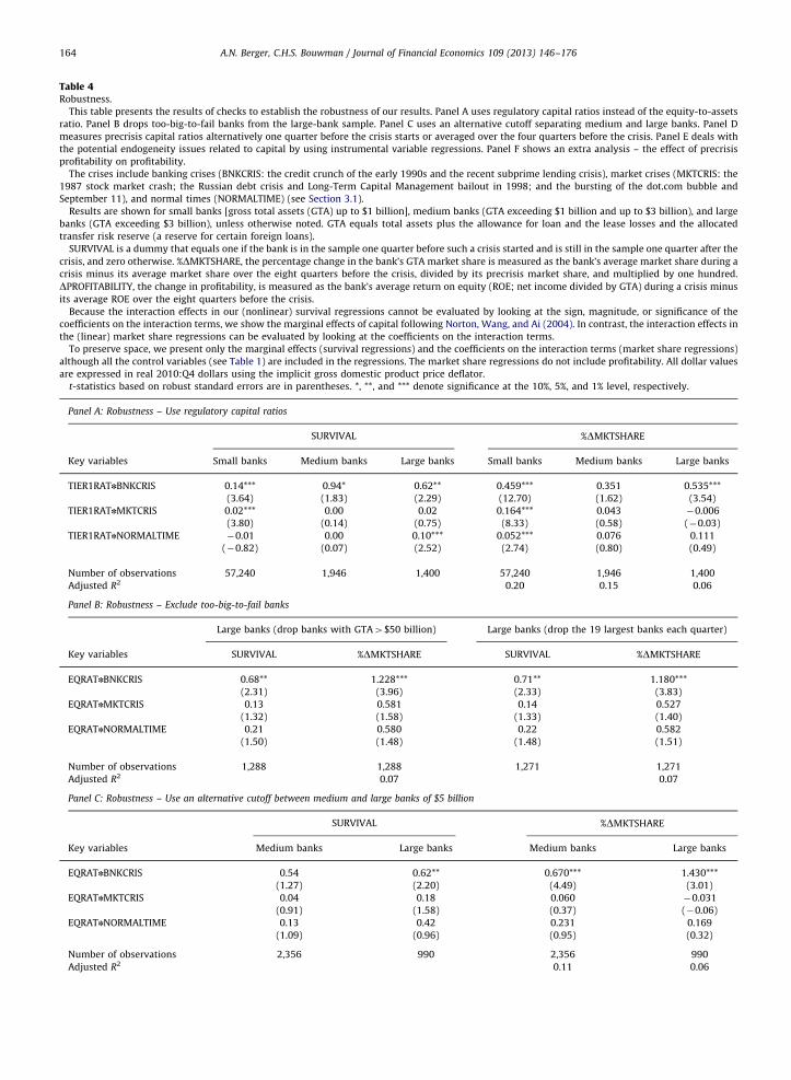
Table 4Robustness.

This table presents the results of checks to establish the robustness of our results. Panel A uses regulatory capital ratios instead of the equity-to-assets

ratio. Panel B drops too-big-to-fail banks from the large-bank sample. Panel C uses an alternative cutoff separating medium and large banks. Panel D

measures precrisis capital ratios alternatively one quarter before the crisis starts or averaged over the four quarters before the crisis. Panel E deals with

the potential endogeneity issues related to capital by using instrumental variable regressions. Panel F shows an extra analysis – the effect of precrisis

profitability on profitability.

The crises include banking crises (BNKCRIS: the credit crunch of the early 1990s and the recent subprime lending crisis), market crises (MKTCRIS: the

1987 stock market crash; the Russian debt crisis and Long-Term Capital Management bailout in 1998; and the bursting of the dot.com bubble and

September 11), and normal times (NORMALTIME) (see Section 3.1).

Results are shown for small banks [gross total assets (GTA) up to $1 billion], medium banks (GTA exceeding $1 billion and up to $3 billion), and large

banks (GTA exceeding $3 billion), unless otherwise noted. GTA equals total assets plus the allowance for loan and the lease losses and the allocated

transfer risk reserve (a reserve for certain foreign loans).

SURVIVAL is a dummy that equals one if the bank is in the sample one quarter before such a crisis started and is still in the sample one quarter after the

crisis, and zero otherwise. %DMKTSHARE, the percentage change in the bank’s GTA market share is measured as the bank’s average market share during a

crisis minus its average market share over the eight quarters before the crisis, divided by its precrisis market share, and multiplied by one hundred.

DPROFITABILITY, the change in profitability, is measured as the bank’s average return on equity (ROE; net income divided by GTA) during a crisis minus

its average ROE over the eight quarters before the crisis.

Because the interaction effects in our (nonlinear) survival regressions cannot be evaluated by looking at the sign, magnitude, or significance of the

coefficients on the interaction terms, we show the marginal effects of capital following Norton, Wang, and Ai (2004). In contrast, the interaction effects in

the (linear) market share regressions can be evaluated by looking at the coefficients on the interaction terms.

To preserve space, we present only the marginal effects (survival regressions) and the coefficients on the interaction terms (market share regressions)

although all the control variables (see Table 1) are included in the regressions. The market share regressions do not include profitability. All dollar values

are expressed in real 2010:Q4 dollars using the implicit gross domestic product price deflator.

t-statistics based on robust standard errors are in parentheses. *, **, and *** denote significance at the 10%, 5%, and 1% level, respectively.

Panel A: Robustness – Use regulatory capital ratios

SURVIVAL %DMKTSHARE

Key variables Small banks Medium banks Large banks Small banks Medium banks Large banks

TIER1RATnBNKCRIS 0.14*** 0.94* 0.62** 0.459*** 0.351 0.535***

(3.64) (1.83) (2.29) (12.70) (1.62) (3.54)

TIER1RATnMKTCRIS 0.02*** 0.00 0.02 0.164*** 0.043 �0.006

(3.80) (0.14) (0.75) (8.33) (0.58) (�0.03)

TIER1RATnNORMALTIME �0.01 0.00 0.10*** 0.052*** 0.076 0.111

(�0.82) (0.07) (2.52) (2.74) (0.80) (0.49)

Number of observations 57,240 1,946 1,400 57,240 1,946 1,400

Adjusted R2 0.20 0.15 0.06

Panel B: Robustness – Exclude too-big-to-fail banks

Large banks (drop banks with GTA4$50 billion) Large banks (drop the 19 largest banks each quarter)

Key variables SURVIVAL %DMKTSHARE SURVIVAL %DMKTSHARE

EQRATnBNKCRIS 0.68** 1.228*** 0.71** 1.180***

(2.31) (3.96) (2.33) (3.83)

EQRATnMKTCRIS 0.13 0.581 0.14 0.527

(1.32) (1.58) (1.33) (1.40)

EQRATnNORMALTIME 0.21 0.580 0.22 0.582

(1.50) (1.48) (1.48) (1.51)

Number of observations 1,288 1,288 1,271 1,271

Adjusted R2 0.07 0.07

Panel C: Robustness – Use an alternative cutoff between medium and large banks of $5 billion

SURVIVAL %DMKTSHARE

Key variables Medium banks Large banks Medium banks Large banks

EQRATnBNKCRIS 0.54 0.62** 0.670*** 1.430***

(1.27) (2.20) (4.49) (3.01)

EQRATnMKTCRIS 0.04 0.18 0.060 �0.031

(0.91) (1.58) (0.37) (�0.06)

EQRATnNORMALTIME 0.13 0.42 0.231 0.169

(1.09) (0.96) (0.95) (0.32)

Number of observations 2,356 990 2,356 990

Adjusted R2 0.11 0.06

A.N. Berger, C.H.S. Bouwman / Journal of Financial Economics 109 (2013) 146–176164

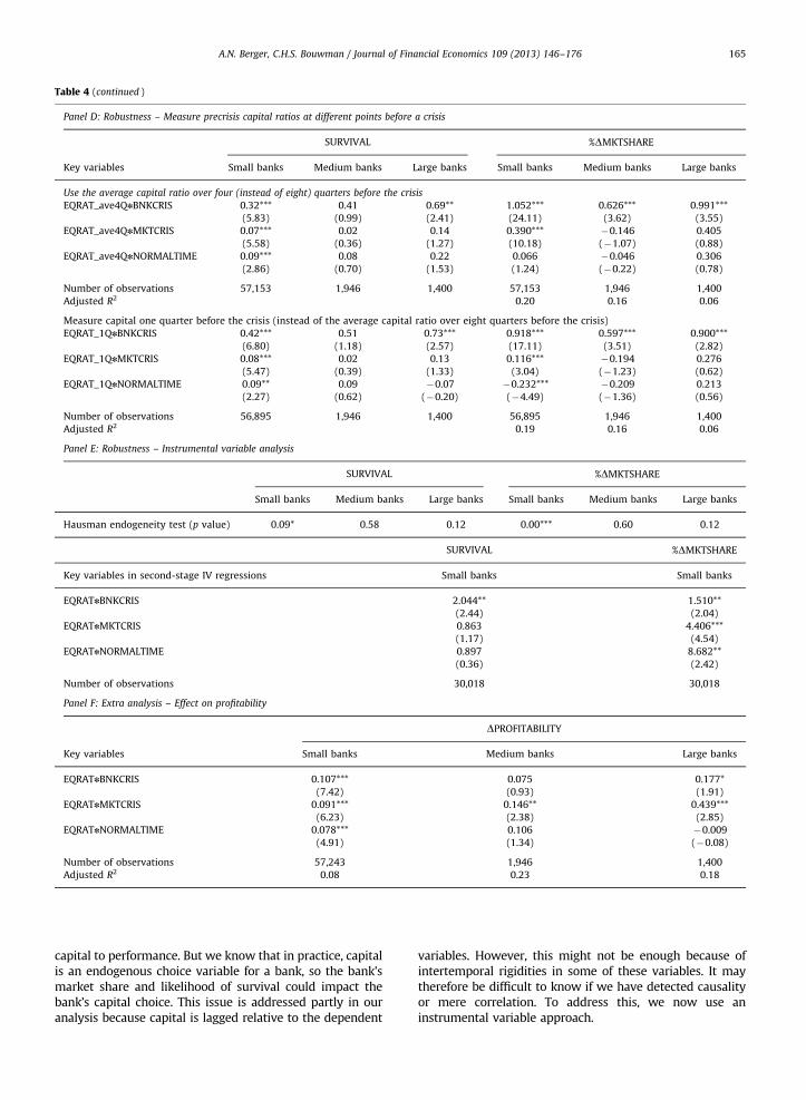
Table 4 (continued )

Panel D: Robustness – Measure precrisis capital ratios at different points before a crisis

SURVIVAL %DMKTSHARE

Key variables Small banks Medium banks Large banks Small banks Medium banks Large banks

Use the average capital ratio over four (instead of eight) quarters before the crisis

EQRAT_ave4QnBNKCRIS 0.32*** 0.41 0.69** 1.052*** 0.626*** 0.991***

(5.83) (0.99) (2.41) (24.11) (3.62) (3.55)

EQRAT_ave4QnMKTCRIS 0.07*** 0.02 0.14 0.390*** �0.146 0.405

(5.58) (0.36) (1.27) (10.18) (�1.07) (0.88)

EQRAT_ave4QnNORMALTIME 0.09*** 0.08 0.22 0.066 �0.046 0.306

(2.86) (0.70) (1.53) (1.24) (�0.22) (0.78)

Number of observations 57,153 1,946 1,400 57,153 1,946 1,400

Adjusted R2 0.20 0.16 0.06

Measure capital one quarter before the crisis (instead of the average capital ratio over eight quarters before the crisis)

EQRAT_1QnBNKCRIS 0.42*** 0.51 0.73*** 0.918*** 0.597*** 0.900***

(6.80) (1.18) (2.57) (17.11) (3.51) (2.82)

EQRAT_1QnMKTCRIS 0.08*** 0.02 0.13 0.116*** �0.194 0.276

(5.47) (0.39) (1.33) (3.04) (�1.23) (0.62)

EQRAT_1QnNORMALTIME 0.09** 0.09 �0.07 �0.232*** �0.209 0.213

(2.27) (0.62) (�0.20) (�4.49) (�1.36) (0.56)

Number of observations 56,895 1,946 1,400 56,895 1,946 1,400

Adjusted R2 0.19 0.16 0.06

Panel E: Robustness – Instrumental variable analysis

SURVIVAL %DMKTSHARE

Small banks Medium banks Large banks Small banks Medium banks Large banks

Hausman endogeneity test (p value) 0.09* 0.58 0.12 0.00*** 0.60 0.12

SURVIVAL %DMKTSHARE

Key variables in second-stage IV regressions Small banks Small banks

EQRATnBNKCRIS 2.044** 1.510**

(2.44) (2.04)

EQRATnMKTCRIS 0.863 4.406***

(1.17) (4.54)

EQRATnNORMALTIME 0.897 8.682**

(0.36) (2.42)

Number of observations 30,018 30,018

Panel F: Extra analysis – Effect on profitability

DPROFITABILITY

Key variables Small banks Medium banks Large banks

EQRATnBNKCRIS 0.107*** 0.075 0.177*

(7.42) (0.93) (1.91)

EQRATnMKTCRIS 0.091*** 0.146** 0.439***

(6.23) (2.38) (2.85)

EQRATnNORMALTIME 0.078*** 0.106 �0.009

(4.91) (1.34) (�0.08)

Number of observations 57,243 1,946 1,400

Adjusted R2 0.08 0.23 0.18

A.N. Berger, C.H.S. Bouwman / Journal of Financial Economics 109 (2013) 146–176 165

capital to performance. But we know that in practice, capitalis an endogenous choice variable for a bank, so the bank’smarket share and likelihood of survival could impact thebank’s capital choice. This issue is addressed partly in ouranalysis because capital is lagged relative to the dependent

variables. However, this might not be enough because ofintertemporal rigidities in some of these variables. It maytherefore be difficult to know if we have detected causalityor mere correlation. To address this, we now use aninstrumental variable approach.

A.N. Berger, C.H.S. Bouwman / Journal of Financial Economics 109 (2013) 146–176166

If our survival and market share regressions includedcapital per se (instead of capital–crisis interaction terms),we could simply select an instrument for capital. Becauseour regressions include capital interacted with three crisisdummies (EQRATnBNKCRIS, EQRATnMKTCRIS, and EQRATnNORMALTIME), we have three potentially endogenousvariables and need an instrument for each interactionterm.24 We employ three instruments in each regression.For reasons explained below, we employ different instru-ments for banks of different sizes. Specifically, for smalland medium banks, we use SENIORS, the fraction of peopleaged 65 and over in the markets in which a bank is active,interacted with the three crisis dummies; for large banks,we use EFF-TAX, the effective state income tax rate a bankhas to pay, interacted with the three crisis dummies.

This instrumentation strategy assumes that SENIORSand EFF-TAX are correlated with the amount of capital(instrument relevance), but do not directly affect perfor-mance (exclusion restriction). Both variables, used byBerger and Bouwman (2009) as instruments for capital,seem to meet these conditions. Consider SENIORS first.Seniors own larger equity portfolios than the averagefamily. Furthermore, using US data, Coval and Moskowitz(1999) find that investors have a strong preference forinvesting close to home. This preference is greater for firmsthat are smaller, more highly levered, and those producinggoods that are not traded internationally. This evidencesuggests that banks, particularly small and medium banks,operating in markets with more seniors have easier accessto equity financing and hence will operate with highercapital ratios [see Berger and Bouwman (2009) for empiri-cal evidence]. We calculate the fraction of seniors usingmarket-level population data from the 1990, 2000, and2010 decennial Censuses, and we apply these fractions tobank data from 1985 to 1994, 1995 to 2004, and 2005 to2010, respectively. If a bank operates in multiple markets,we use the bank’s deposit-weighted-average fraction ofseniors across its markets.

Although the exclusion restriction is an identifyingrestriction that cannot be tested, one may worry that it isnot satisfied. For example, the fraction of seniors in thebank’s markets could directly affect bank survival throughthe political process. If seniors dislike bank default morethan young people do, they would lobby politicians moreactively. While this is a possibility, we are not aware ofany theories that predict this or of any empiricalor anecdotal evidence supporting this.25 Another concern

24 It is not correct to view EQRAT as the endogenous right-hand-side

variable, create a predicted value of EQRAT in the first stage, and then

interact it with the three crisis dummies in the second stage. Wooldridge

(2002, p. 236) and Angrist and Pischke (2009, pp. 190–192) call this the

‘‘forbidden regression.’’25 While small-bank lobbying tends to be done by associations such

as the Independent Community Bankers of America, which has around

five thousand members, individual shareholders could also lobby poli-

ticians. Evidence on lobbying by age category is hard to obtain, but we

are not aware of any evidence or theoretical argument that older

individuals lobby more. The American Association of Retired Persons

(AARP), one of the most powerful lobbying groups in the US with more

than forty million members, seems to focus primarily on issues related

to enhancing the quality of life for seniors.

is that the fraction of seniors could directly affect marketshares. Seniors may have a preference for certain bankservices and be more loyal than younger customers. Evenif true, however, it would apply to all banks serving amarket with a given fraction of seniors, so it is difficult tosee how operating in a market with more seniors wouldendow a bank with a stronger competitive advantagerelative to other banks operating in the same market, andthus with greater market share.

While SENIORS (interacted with three crisis dummies)can be used for small and medium banks, it is not asattractive for large banks because these banks are unlikelyto be locally-based when it comes to raising equity. Forthis reason, we use EFF-TAX (interacted with three crisisdummies) for large banks. Because interest on debt is tax-deductible and dividend payments are not, banks thatoperate in states with higher income tax rates areexpected to have lower equity ratios, all else equal (e.g.,Ashcraft, 2008; Berger and Bouwman, 2009). Similar toAshcraft (2008), we define EFF-TAX as the effectiveincome tax rate to be paid on $1 million in pretax income.If a bank operates in multiple states, we use the bank’sweighted-average state income tax rate, calculated usingthe bank’s share of deposits in each state as weights.

Because ordinary least squares is preferred to instru-mental variable regressions if we do not have an endo-geneity problem, we perform Hausman tests forendogeneity. As shown in Table 4, Panel E, we do notreject the null that the three potentially endogenousvariables are exogenous for medium and large banks,suggesting that our original analyses were appropriatefor these banks. However, we do find evidence of endo-geneity for small banks and therefore perform instru-mental variable regressions only for those banks.

Since our small-bank survival regressions have threeendogenous variables, we run three first-stage regressions.We regress EQRATnBNKCRIS on all the exogenous variablesused in our survival regressions plus the three instruments(SENIORS interacted with the three crisis dummies; first-stage regression #1), and do the same using EQRATnMKT-CRIS (first-stage regression #2) and EQRATnNORMALTIME(first-stage regression #3). In similar vein, we also runthree first-stage regressions for our small-bank marketshare regressions. The survival and market share first-stage regressions are slightly different because the survivalregressions include profitability as a control variable whilethe market share regressions do not.

Importantly, when EQRATnBNKCRIS is the endogenousvariable (first-stage regression #1), the coefficient on thecorresponding instrument (SENIORSnBNKCRIS) is highlysignificant. We obtain similar results for the other twoendogenous variables in first-stage regressions #2 and #3(not shown for brevity).

If the instruments are weak (the correlation with theendogenous regressors is low), IV estimates are biasedtoward the OLS estimates in finite samples (e.g., Bound,Jaeger, and Baker, 1995; Staiger and Stock, 1997). To verifythat this is not a problem, we calculate the Angrist-Pischkefirst-stage F-statistic of excluded instruments for every first-stage regression to test the hypothesis that all instrumentcoefficients are zero (Angrist and Pischke, 2009). The

A.N. Berger, C.H.S. Bouwman / Journal of Financial Economics 109 (2013) 146–176 167

associated p-values range from 0.00 to 0.01, suggesting we donot have a weak instrument problem.

We run two small-bank second-stage regressions. Weregress SURVIVAL on the predicted values of the threeendogenous variables from the first stage and all the controlvariables and fixed effects, and we run a comparable regres-sion using %DMKTSHARE as the dependent variable. Table 4,Panel E, shows the two second-stage regressions. Usinginstruments, we find that capital helps small banks survivebanking crises only, and helps them improve their marketshares at all times. Thus, most of our earlier results hold up inour instrumental variable analysis, and the analysis broadlyconfirms our main results.

5.6. Extra analysis: the effects of capital on profitability

Our results suggest that capital helps small banks tosurvive and improve their market shares at all times, andit helps medium and large banks during banking crisesonly. It is interesting to see if these benefits of capital helpbanks improve their profitability as well. Several theorypapers suggest that higher capital should enhance profit-ability (e.g., Holmstrom and Tirole, 1997; Allen, Carletti,and Marquez, 2011; Mehran and Thakor, 2011), whileothers argue that it should (mechanically) lead to areduced return on equity (e.g., Modigliani and Miller,1963). Acharya and Mora (2011) find that banks bid morefor deposits during a financial crisis, which could lowerprofitability. Berger (1995) finds that the relation betweencapital and earnings can be positive or negative but, likethe theory papers, does not differentiate between finan-cial crises and normal times.

We measure a bank’s profitability using the bank’sROE.26 To examine whether a bank improves its profit-ability during banking crises, market crises, and normaltimes, we focus on the change in ROE (DROE), defined asthe bank’s average profitability during these crises minusthe bank’s average ROE over the eight quarters beforethese crises. We regress DROE on the bank’s precrisiscapital ratio plus the same set of control variables that isincluded in the market share regressions.

Table 4, Panel F, contains the results. We have twomain findings. First, capital enhances the profitability ofsmall banks at all times (during banking crises, marketcrises, and normal times). Second, capital improves theprofitability of medium and large banks during bankingcrises (not significant for medium banks) and marketcrises. Thus, capital generally improves bank profitability.

6. Regression results based on individual crises

The main regressions group the two banking crisestogether and the three market crises together. This

26 If a bank’s capital to GTA ratio is less than 1%, we calculate ROE as

net income divided by 1% of GTA. For observations for which equity is

between 0% and 1% of GTA, dividing by equity would result in extra-

ordinarily high values. For observations for which equity is negative, the

conventionally-defined ROE would not make economic sense. We do not

drop these negative-equity observations because they are likely infor-

mative of banks’ ability to survive crises.

approach facilitates drawing general conclusions abouthow the role of capital differs across banking crises andmarket crises, while minimizing the impact of the idio-syncratic circumstances surrounding a particular crisis.This is useful because the specific attributes of a crisis areunknown before the crisis strikes. Aggregating acrossbanking crises and across market crises allows us togenerate a comprehensive picture of specific types ofcrises, thereby leading to a better predictive frameworkfor extrapolation for future crises.

However, an advantage of looking at individual crisesis that it permits a more granular look at how the role ofcapital is affected by the specific circumstances of thatcrisis. That is, there is value in also understanding if therole of capital is influenced by the details of a given crisis,including its origins and the extent of government inter-vention. For example, each banking crisis has features thatit shares with other banking crises but also features thatwere peculiar to that crisis. The credit crunch wasattributed in part to the transition of capital requirementsto Basel I’s risk-based scheme (e.g., Hancock, Laing, andWilcox, 1995; Thakor, 1996), whereas the subprime crisiswas triggered in part by unexpectedly large defaults onsubprime mortgages (e.g., Gorton and Metrick, 2012a,2012b). In addition, the credit crunch took place duringa period of intense industry consolidation, while thesubprime lending crisis involved unprecedented interven-tion by the Federal Reserve and the Treasury. We there-fore rerun the main regressions and the robustness checksseparately for each of the five crises and normal times. Weexclude the individual crisis dummies and drop somecontrols from our survival regressions to avoid collinear-ity. We drop these variables from the market shareregressions for those size classes as well for consistency.The table indicates which control variables are included.27

Table 5 contains the main results based on individualcrises. Capital helps small banks survive at virtually alltimes (both banking crises, two out of the three marketcrises, and during normal times) and helps them improvetheir market shares during every crisis and during normaltimes. In contrast, capital helps medium and large bankssurvive only one of the banking crises (the credit crunch)and also helps them improve their competitive positionduring both banking crises.

The robustness checks using individual crises yieldresults that are very similar to the main individual crisisresults (not shown for brevity; the results are availableupon request).28

These results suggest that capital is a significantfacilitator for small banks during every crisis and duringnormal times. It benefited medium and large banks in

27 The survival regressions are run only for cases in which there are

a sufficient number of non-survivors. As a result, regressions are not run

for medium and large banks during CRIS1, and for large banks during

CRIS3. These cases are indicated as n/a.28 The individual crisis IV results for small banks show that the

instrument is positively and significantly related to capital in four out of

five crises (not significant during the recent crisis). In the second stage,

capital is positively related to survival and market share in virtually

every crisis, but not always significant.

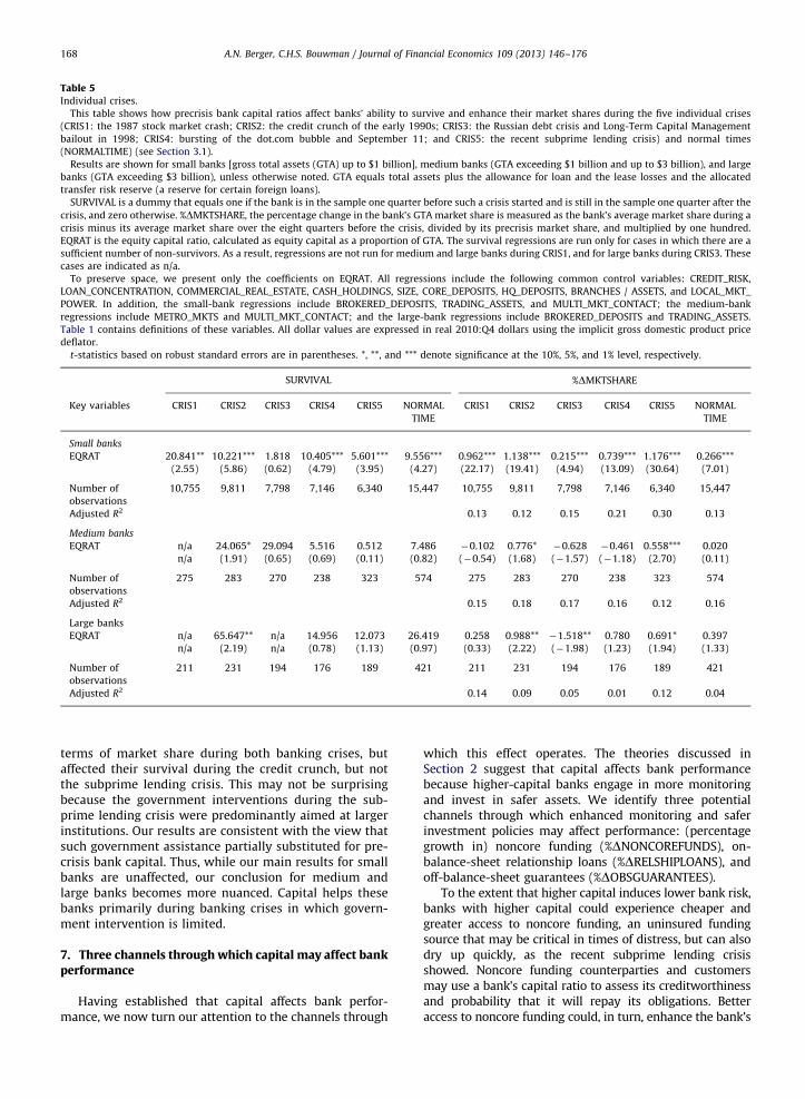
Table 5Individual crises.

This table shows how precrisis bank capital ratios affect banks’ ability to survive and enhance their market shares during the five individual crises

(CRIS1: the 1987 stock market crash; CRIS2: the credit crunch of the early 1990s; CRIS3: the Russian debt crisis and Long-Term Capital Management

bailout in 1998; CRIS4: bursting of the dot.com bubble and September 11; and CRIS5: the recent subprime lending crisis) and normal times

(NORMALTIME) (see Section 3.1).

Results are shown for small banks [gross total assets (GTA) up to $1 billion], medium banks (GTA exceeding $1 billion and up to $3 billion), and large

banks (GTA exceeding $3 billion), unless otherwise noted. GTA equals total assets plus the allowance for loan and the lease losses and the allocated

transfer risk reserve (a reserve for certain foreign loans).

SURVIVAL is a dummy that equals one if the bank is in the sample one quarter before such a crisis started and is still in the sample one quarter after the

crisis, and zero otherwise. %DMKTSHARE, the percentage change in the bank’s GTA market share is measured as the bank’s average market share during a

crisis minus its average market share over the eight quarters before the crisis, divided by its precrisis market share, and multiplied by one hundred.

EQRAT is the equity capital ratio, calculated as equity capital as a proportion of GTA. The survival regressions are run only for cases in which there are a

sufficient number of non-survivors. As a result, regressions are not run for medium and large banks during CRIS1, and for large banks during CRIS3. These

cases are indicated as n/a.

To preserve space, we present only the coefficients on EQRAT. All regressions include the following common control variables: CREDIT_RISK,

LOAN_CONCENTRATION, COMMERCIAL_REAL_ESTATE, CASH_HOLDINGS, SIZE, CORE_DEPOSITS, HQ_DEPOSITS, BRANCHES / ASSETS, and LOCAL_MKT_

POWER. In addition, the small-bank regressions include BROKERED_DEPOSITS, TRADING_ASSETS, and MULTI_MKT_CONTACT; the medium-bank

regressions include METRO_MKTS and MULTI_MKT_CONTACT; and the large-bank regressions include BROKERED_DEPOSITS and TRADING_ASSETS.

Table 1 contains definitions of these variables. All dollar values are expressed in real 2010:Q4 dollars using the implicit gross domestic product price

deflator.

t-statistics based on robust standard errors are in parentheses. *, **, and *** denote significance at the 10%, 5%, and 1% level, respectively.

SURVIVAL %DMKTSHARE

Key variables CRIS1 CRIS2 CRIS3 CRIS4 CRIS5 NORMAL

TIME

CRIS1 CRIS2 CRIS3 CRIS4 CRIS5 NORMAL

TIME

Small banks

EQRAT 20.841** 10.221*** 1.818 10.405*** 5.601*** 9.556*** 0.962*** 1.138*** 0.215*** 0.739*** 1.176*** 0.266***

(2.55) (5.86) (0.62) (4.79) (3.95) (4.27) (22.17) (19.41) (4.94) (13.09) (30.64) (7.01)

Number of

observations

10,755 9,811 7,798 7,146 6,340 15,447 10,755 9,811 7,798 7,146 6,340 15,447

Adjusted R2 0.13 0.12 0.15 0.21 0.30 0.13

Medium banks

EQRAT n/a 24.065* 29.094 5.516 0.512 7.486 �0.102 0.776* �0.628 �0.461 0.558*** 0.020

n/a (1.91) (0.65) (0.69) (0.11) (0.82) (�0.54) (1.68) (�1.57) (�1.18) (2.70) (0.11)

Number of

observations

275 283 270 238 323 574 275 283 270 238 323 574

Adjusted R2 0.15 0.18 0.17 0.16 0.12 0.16

Large banks

EQRAT n/a 65.647** n/a 14.956 12.073 26.419 0.258 0.988** �1.518** 0.780 0.691* 0.397

n/a (2.19) n/a (0.78) (1.13) (0.97) (0.33) (2.22) (�1.98) (1.23) (1.94) (1.33)

Number of

observations

211 231 194 176 189 421 211 231 194 176 189 421

Adjusted R2 0.14 0.09 0.05 0.01 0.12 0.04

A.N. Berger, C.H.S. Bouwman / Journal of Financial Economics 109 (2013) 146–176168

terms of market share during both banking crises, butaffected their survival during the credit crunch, but notthe subprime lending crisis. This may not be surprisingbecause the government interventions during the sub-prime lending crisis were predominantly aimed at largerinstitutions. Our results are consistent with the view thatsuch government assistance partially substituted for pre-crisis bank capital. Thus, while our main results for smallbanks are unaffected, our conclusion for medium andlarge banks becomes more nuanced. Capital helps thesebanks primarily during banking crises in which govern-ment intervention is limited.

7. Three channels through which capital may affect bankperformance

Having established that capital affects bank perfor-mance, we now turn our attention to the channels through

which this effect operates. The theories discussed inSection 2 suggest that capital affects bank performancebecause higher-capital banks engage in more monitoringand invest in safer assets. We identify three potentialchannels through which enhanced monitoring and saferinvestment policies may affect performance: (percentagegrowth in) noncore funding (%DNONCOREFUNDS), on-balance-sheet relationship loans (%DRELSHIPLOANS), andoff-balance-sheet guarantees (%DOBSGUARANTEES).

To the extent that higher capital induces lower bank risk,banks with higher capital could experience cheaper andgreater access to noncore funding, an uninsured fundingsource that may be critical in times of distress, but can alsodry up quickly, as the recent subprime lending crisisshowed. Noncore funding counterparties and customersmay use a bank’s capital ratio to assess its creditworthinessand probability that it will repay its obligations. Betteraccess to noncore funding could, in turn, enhance the bank’s

A.N. Berger, C.H.S. Bouwman / Journal of Financial Economics 109 (2013) 146–176 169

survival probability and market share. We calculate noncorefunding as total liabilities minus stockholders equity andcore deposits (as defined in Section 3.2).

More monitoring and safer investments associatedwith higher capital could also improve a bank’s abilityto make relationship loans (e.g., Boot and Thakor, 2000).This may be because relationship borrowers, who ben-efit from long-term interactions with the bank, wouldprefer a bank with higher capital and higher odds ofsurvival, all else equal. This might not only improve thebank’s lending margins, but also enhance loan volume,thereby increasing market share. Moreover, it wouldprovide the balance-sheet stability that is valuable forsurvival. If we had loan-level data, we could construct arelationship loan measure based on duration and scope,two dimensions deemed important in the relationshiplending literature (e.g., Boot, 2000; Ongena and Smith,2000; Degryse and Ongena, 2007). If we had firm-leveldata, we could calculate the bank’s share of the firm’stotal debt (e.g., Presbitero and Zazzaro, 2011). Becausewe only have Call Report data, we use a more crudemeasure and view total loans excluding loans to deposi-tory institutions, foreign governments, and states asrelationship loans.

Buyers of off-balance-sheet guarantees are more likelyto buy claims from less risky, more reputable banks. Boot,Greenbaum, and Thakor (1993) predict this, and higherfinancial capital stochastically elevates reputational capitalin their model. This suggests that higher-capital banks couldgain a competitive advantage over lower-capital peersthrough this off-balance-sheet channel as well. We calculateoff-balance-sheet guarantees as the sum of loan commit-ments and commercial and standby letters of credit.

To assess whether capital affects performancethrough these three channels, we regress each channelon the three capital–crisis interaction terms plus thesame controls as those included in the main regres-sions. Based on the discussion above, we should findthat higher precrisis capital ratios help banks increasetheir noncore funding, on-balance-sheet relationshiploans, and off-balance-sheet guarantees, and this effectis likely to be stronger during financial crises thanduring normal times.

Table 6, Panel A, contains summary statistics, and Panel Bshows the results. As expected, banks with more precrisiscapital show higher growth in noncore funding, relationshiploans, and off-balance-sheet guarantees during the crisis.Interestingly, this seems to hold for small banks at all times,and for medium and large banks primarily during bankingcrises—the cases in which capital helps banks survive andimprove their market shares.

8. Additional analyses

We perform two additional analyses to deepen ourunderstanding of how capital affects bank performance.

8.1. The effects of capital on the manner of exit

We first examine the manner of exit for nonsurviv-ing banks to see whether they are also related to

precrisis capital ratios. To address this, we focus onobservations for which SURV equals zero, i.e., banksthat were alive one quarter before the crisis, butceased to exist one quarter after the crisis.

Table 7, Panel A, contains summary statistics. As canbe seen, 926 of our sample banks exited during bank-ing crises, 461 exited during market crises, and 365exited during normal times (i.e., during the fakecrises). The data show that banks exit in one of thefollowing three ways. First, they were acquired ormerged without government assistance. Dependingon bank size, regular M&As accounted for 26–47% ofall exits during banking crises; 81–86% during marketcrises, and 83–100% during normal times. Second,banks ceased to exist because they were acquired ormerged with government assistance. Not surprisingly,such deals were especially prevalent during bankingcrises, accounting for 48–61% of all exits during thosecrises. During market crises and normal times, only 0–9% and 0–2%, respectively, merge with assistance.Third, banks ceased to exist because they failed out-right or simply changed their charters. In the lattercase, banks merely begin to operate under a newcharter. Unfortunately, the data do not allow us todistinguish between outright failure and change ofcharter. We therefore provide only summary statisticsbut do not perform any further analyses for thiscategory. This type of nonsurvival was not very pre-valent. During banking crises, market crises, and nor-mal times, the percentages ranged from 5–13%, 6–15%,and 0–17%, respectively.

To examine whether conditional on not surviving acrisis, the bank’s precrisis capitalization affects the like-lihood of exit via M&A without or with assistance, we runthe following logit regressions:

EXIT_UNASSISTi ¼ logProbðUNASSISTiÞ

1�ProbðUNASSISTiÞ

� �

¼ a6 þ b6 n EQRATi þ B6 n Zi ð4Þ

and

EXIT_ASSISTi ¼ logProbðASSISTiÞ

1�ProbðASSISTiÞ

� �

¼ a7 þ b7 n EQRATi þ B7 n Zi ð5Þ

where UNASSISTi and ASSISTi are dummy variables thatequal one if bank i was in the sample during the last quarterbefore a crisis but ceased to exist by the first quarter afterthe crisis because it merged or was acquired withoutassistance, and merged or was acquired with governmentassistance, respectively. EQRATi is as defined above. Zi is aset of control variables (see Table 7 for a list) which, toprevent collinearity, includes fewer variables than the mainset Xi. The regressions are run only for cases in which thereare a sufficient number of M&As. As a result, regressions arenot run for medium and large banks (with or withoutassistance) during market crises and normal times, and forsmall banks (with assistance) during normal times. Thesecases are indicated below as n/a.

Table 7, Panel B, contains the results. The EXIT_UNASSISTregressions show that banks with higher capital ratios aremore likely to be acquired via M&A without assistance during

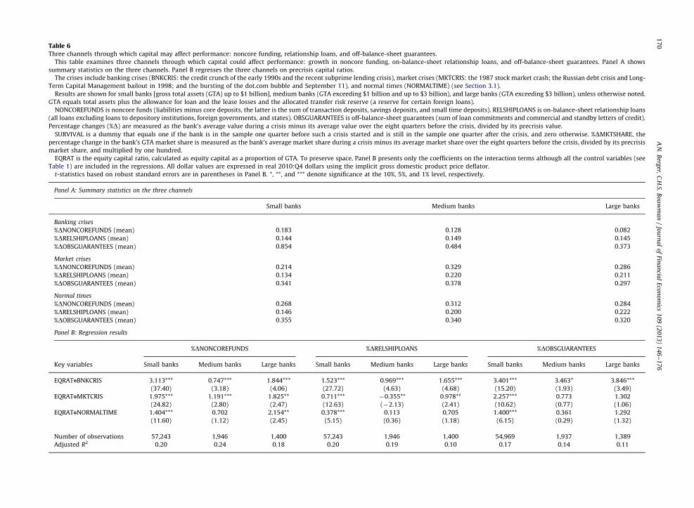
Table 6Three channels through which capital may affect performance: noncore funding, relationship loans, and off-balance-sheet guarantees.

This table examines three channels through which capital could affect performance: growth in noncore funding, on-balance-sheet relationship loans, and off-balance-sheet guarantees. Panel A shows

summary statistics on the three channels. Panel B regresses the three channels on precrisis capital ratios.

The crises include banking crises (BNKCRIS: the credit crunch of the early 1990s and the recent subprime lending crisis), market crises (MKTCRIS: the 1987 stock market crash; the Russian debt crisis and Long-

Term Capital Management bailout in 1998; and the bursting of the dot.com bubble and September 11), and normal times (NORMALTIME) (see Section 3.1).

Results are shown for small banks [gross total assets (GTA) up to $1 billion], medium banks (GTA exceeding $1 billion and up to $3 billion), and large banks (GTA exceeding $3 billion), unless otherwise noted.

GTA equals total assets plus the allowance for loan and the lease losses and the allocated transfer risk reserve (a reserve for certain foreign loans).

NONCOREFUNDS is noncore funds (liabilities minus core deposits, the latter is the sum of transaction deposits, savings deposits, and small time deposits). RELSHIPLOANS is on-balance-sheet relationship loans

(all loans excluding loans to depository institutions, foreign governments, and states). OBSGUARANTEES is off-balance-sheet guarantees (sum of loan commitments and commercial and standby letters of credit).

Percentage changes (%D) are measured as the bank’s average value during a crisis minus its average value over the eight quarters before the crisis, divided by its precrisis value.

SURVIVAL is a dummy that equals one if the bank is in the sample one quarter before such a crisis started and is still in the sample one quarter after the crisis, and zero otherwise. %DMKTSHARE, the

percentage change in the bank’s GTA market share is measured as the bank’s average market share during a crisis minus its average market share over the eight quarters before the crisis, divided by its precrisis

market share, and multiplied by one hundred.

EQRAT is the equity capital ratio, calculated as equity capital as a proportion of GTA. To preserve space, Panel B presents only the coefficients on the interaction terms although all the control variables (see

Table 1) are included in the regressions. All dollar values are expressed in real 2010:Q4 dollars using the implicit gross domestic product price deflator.

t-statistics based on robust standard errors are in parentheses in Panel B. *, **, and *** denote significance at the 10%, 5%, and 1% level, respectively.

Panel A: Summary statistics on the three channels

Small banks Medium banks Large banks

Banking crises

%DNONCOREFUNDS (mean) 0.183 0.128 0.082

%DRELSHIPLOANS (mean) 0.144 0.149 0.145

%DOBSGUARANTEES (mean) 0.854 0.484 0.373

Market crises

%DNONCOREFUNDS (mean) 0.214 0.329 0.286

%DRELSHIPLOANS (mean) 0.134 0.220 0.211

%DOBSGUARANTEES (mean) 0.341 0.378 0.297

Normal times

%DNONCOREFUNDS (mean) 0.268 0.312 0.284

%DRELSHIPLOANS (mean) 0.146 0.200 0.222

%DOBSGUARANTEES (mean) 0.355 0.340 0.320

Panel B: Regression results

%DNONCOREFUNDS %DRELSHIPLOANS %DOBSGUARANTEES

Key variables Small banks Medium banks Large banks Small banks Medium banks Large banks Small banks Medium banks Large banks

EQRATnBNKCRIS 3.113*** 0.747*** 1.844*** 1.523*** 0.969*** 1.655*** 3.401*** 3.463* 3.846***

(37.40) (3.18) (4.06) (27.72) (4.63) (4.68) (15.20) (1.93) (3.49)

EQRATnMKTCRIS 1.975*** 1.191*** 1.825** 0.711*** �0.355** 0.978** 2.257*** 0.773 1.302

(24.82) (2.80) (2.47) (12.63) (�2.13) (2.41) (10.62) (0.77) (1.06)

EQRATnNORMALTIME 1.404*** 0.702 2.154** 0.378*** 0.113 0.705 1.400*** 0.361 1.292

(11.60) (1.12) (2.45) (5.15) (0.36) (1.18) (6.15) (0.29) (1.32)

Number of observations 57,243 1,946 1,400 57,243 1,946 1,400 54,969 1,937 1,389

Adjusted R2 0.20 0.24 0.18 0.20 0.19 0.10 0.17 0.14 0.11

A.N

.B

erger,

C.H

.S.B

ou

wm

an

/Jo

urn

al

of

Fina

ncia

lE

con

om

ics1

09

(20

13

)1

46

–1

76

17

0

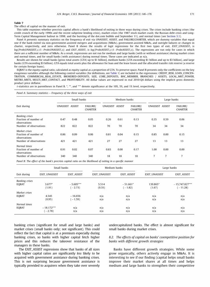
Table 7The effect of capital on the manner of exit.

This table examines whether precrisis capital affects a bank’s likelihood of exiting in three ways during crises. The crises include banking crises (the

credit crunch of the early 1990s and the recent subprime lending crisis), market crises (the 1987 stock market crash; the Russian debt crisis and Long-

Term Capital Management bailout in 1998; and the bursting of the dot.com bubble and September 11), and normal times (see Section 3.1).

Panel A presents summary statistics on the frequency of exit via UNASSIST, ASSIST, and FAILURE/CHARTER, which are dummy variables that equal

one if the bank exited via non-government-assisted mergers and acquisitions (M&As), government-assisted M&As, and outright failures or changes in

charter, respectively, and zero otherwise. Panel B shows the results of logit regressions for the first two types of exit. EXIT_UNASSISTi is

log ProbðUNASSISTiÞ=ð1�ProbðUNASSISTiÞÞ� �

and EXIT_ASSISTi is log ProbðASSISTiÞ=ð1�ProbðASSISTiÞÞ� �

. The regressions are run only for cases in which

there are a sufficient number of M&As. As a result, regressions are not run for medium and large banks (with or without assistance) during market crises

and normal times, and for small banks (with assistance) during normal times. These cases are indicated as n/a.

Results are shown for small banks [gross total assets (GTA) up to $1 billion], medium banks (GTA exceeding $1 billion and up to $3 billion), and large

banks (GTA exceeding $3 billion). GTA equals total assets plus the allowance for loan and the lease losses and the allocated transfer risk reserve (a reserve

for certain foreign loans).

EQRAT is the equity capital ratio, calculated as equity capital as a proportion of GTA. To preserve space, Panel B presents only the coefficients on the key

exogenous variables although the following control variables (for definitions, see Table 1) are included in the regressions: CREDIT_RISK, LOAN_CONCEN-

TRATION, COMMERCIAL_REAL_ESTATE, BROKERED-DEPOSITS, SIZE, CORE_DEPOSITS, BHC_MEMBER, BRANCHES / ASSETS, LOCAL_MKT_POWER,

METRO_MKTS, MULTI_MKT_CONTACT, and PROFITABILITY. All dollar values are expressed in real 2010:Q4 dollars using the implicit gross domestic

product price deflator.

t-statistics are in parentheses in Panel B. *, **, and *** denote significance at the 10%, 5%, and 1% level, respectively.

Panel A: Summary statistics – Frequency of the three ways of exit

Small banks Medium banks Large banks

Exit during UNASSIST ASSIST FAILURE/

CHARTER

UNASSIST ASSIST FAILURE/

CHARTER

UNASSIST ASSIST FAILURE/

CHARTER

Banking crises

Fraction of number of

observations

0.47 0.48 0.05 0.26 0.61 0.13 0.35 0.59 0.06

Number of observations 822 822 822 70 70 70 34 34 34

Market crises

Fraction of number of

observations

0.86 0.09 0.06 0.81 0.04 0.15 0.85 0.00 0.15

Number of observations 421 421 421 27 27 27 13 13 13

Normal times

Fraction of number of

observations

0.91 0.02 0.07 0.83 0.00 0.17 1.00 0.00 0.00

Number of observations 340 340 340 18 18 18 7 7 7

Panel B: The effect of the bank’s precrisis capital ratio on the likelihood of exiting in a specific manner

Small banks Medium banks Large banks

Exit during EXIT_UNASSIST EXIT_ASSIST EXIT_UNASSIST EXIT_ASSIST EXIT_UNASSIST EXIT_ASSIST

Banking crises

EQRAT 3.677* �5.605*** 5.514 �51.661* 139.865* �15,747.827***

(1.91) (�2.73) (0.35) (�1.82) (1.67) (�11.28)

Market crises

EQRAT 4.545 �16.656 n/a n/a n/a n/a

(0.95) (�1.59) n/a n/a n/a n/a

Normal times

EQRAT �18.172*** n/a n/a n/a n/a n/a

(�2.78) n/a n/a n/a n/a n/a

A.N. Berger, C.H.S. Bouwman / Journal of Financial Economics 109 (2013) 146–176 171

banking crises (significant for small and large banks) andmarket crises (small banks only; not significant). This couldreflect the fact that capital is at a premium especially duringbanking crises, so banks with higher capital fetch higherprices and this reduces the takeover resistance of themanagers in these banks.

The EXIT_ASSIST regressions show that banks of all sizeswith higher capital ratios are significantly less likely to beacquired with government assistance during banking crises.This is not surprising because government assistance istypically provided to acquirers when they take over severely

undercapitalized banks. The effect is almost significant forsmall banks during market crises.

8.2. The effects of capital on banks’ coxmpetitive position for

banks with different growth strategies

Banks have different growth strategies. While somegrow organically, others actively engage in M&As. It isinteresting to see if our finding (capital helps small banksimprove their market shares at all times and helpsmedium and large banks to strengthen their competitive

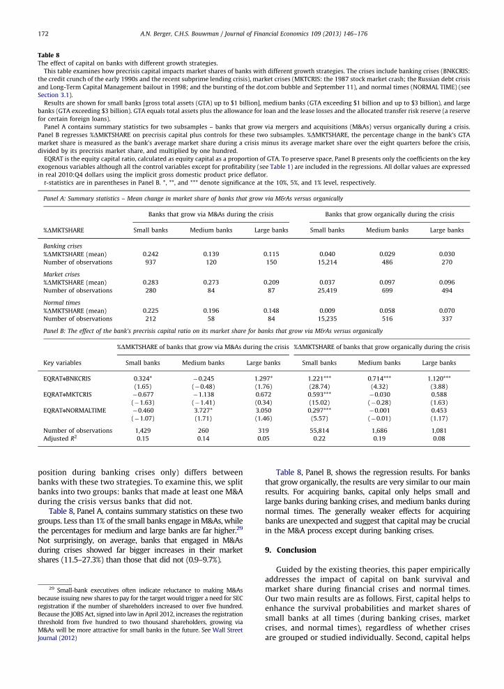
Table 8The effect of capital on banks with different growth strategies.

This table examines how precrisis capital impacts market shares of banks with different growth strategies. The crises include banking crises (BNKCRIS:

the credit crunch of the early 1990s and the recent subprime lending crisis), market crises (MKTCRIS: the 1987 stock market crash; the Russian debt crisis

and Long-Term Capital Management bailout in 1998; and the bursting of the dot.com bubble and September 11), and normal times (NORMAL TIME) (see

Section 3.1).

Results are shown for small banks [gross total assets (GTA) up to $1 billion], medium banks (GTA exceeding $1 billion and up to $3 billion), and large

banks (GTA exceeding $3 billion). GTA equals total assets plus the allowance for loan and the lease losses and the allocated transfer risk reserve (a reserve

for certain foreign loans).

Panel A contains summary statistics for two subsamples – banks that grow via mergers and acquisitions (M&As) versus organically during a crisis.

Panel B regresses %DMKTSHARE on precrisis capital plus controls for these two subsamples. %DMKTSHARE, the percentage change in the bank’s GTA

market share is measured as the bank’s average market share during a crisis minus its average market share over the eight quarters before the crisis,

divided by its precrisis market share, and multiplied by one hundred.

EQRAT is the equity capital ratio, calculated as equity capital as a proportion of GTA. To preserve space, Panel B presents only the coefficients on the key

exogenous variables although all the control variables except for profitability (see Table 1) are included in the regressions. All dollar values are expressed

in real 2010:Q4 dollars using the implicit gross domestic product price deflator.

t-statistics are in parentheses in Panel B. *, **, and *** denote significance at the 10%, 5%, and 1% level, respectively.

Panel A: Summary statistics – Mean change in market share of banks that grow via M&As versus organically

Banks that grow via M&As during the crisis Banks that grow organically during the crisis

%DMKTSHARE Small banks Medium banks Large banks Small banks Medium banks Large banks

Banking crises

%DMKTSHARE (mean) 0.242 0.139 0.115 0.040 0.029 0.030

Number of observations 937 120 150 15,214 486 270

Market crises

%DMKTSHARE (mean) 0.283 0.273 0.209 0.037 0.097 0.096

Number of observations 280 84 87 25,419 699 494

Normal times

%DMKTSHARE (mean) 0.225 0.196 0.148 0.009 0.058 0.070

Number of observations 212 58 84 15,235 516 337

Panel B: The effect of the bank’s precrisis capital ratio on its market share for banks that grow via M&As versus organically

%DMKTSHARE of banks that grow via M&As during the crisis %DMKTSHARE of banks that grow organically during the crisis

Key variables Small banks Medium banks Large banks Small banks Medium banks Large banks

EQRATnBNKCRIS 0.324* �0.245 1.297* 1.221*** 0.714*** 1.120***

(1.65) (�0.48) (1.76) (28.74) (4.32) (3.88)

EQRATnMKTCRIS �0.677 �1.138 0.672 0.593*** �0.030 0.588

(�1.63) (�1.41) (0.34) (15.02) (�0.28) (1.63)

EQRATnNORMALTIME �0.460 3.727* 3.050 0.297*** �0.001 0.453

(�1.07) (1.71) (1.46) (5.57) (�0.01) (1.17)

Number of observations 1,429 260 319 55,814 1,686 1,081

Adjusted R2 0.15 0.14 0.05 0.22 0.19 0.08

A.N. Berger, C.H.S. Bouwman / Journal of Financial Economics 109 (2013) 146–176172

position during banking crises only) differs betweenbanks with these two strategies. To examine this, we splitbanks into two groups: banks that made at least one M&Aduring the crisis versus banks that did not.

Table 8, Panel A, contains summary statistics on these twogroups. Less than 1% of the small banks engage in M&As, whilethe percentages for medium and large banks are far higher.29

Not surprisingly, on average, banks that engaged in M&Asduring crises showed far bigger increases in their marketshares (11.5–27.3%) than those that did not (0.9–9.7%).

29 Small-bank executives often indicate reluctance to making M&As

because issuing new shares to pay for the target would trigger a need for SEC

registration if the number of shareholders increased to over five hundred.

Because the JOBS Act, signed into law in April 2012, increases the registration

threshold from five hundred to two thousand shareholders, growing via

M&As will be more attractive for small banks in the future. See Wall Street

Journal (2012)

Table 8, Panel B, shows the regression results. For banksthat grow organically, the results are very similar to our mainresults. For acquiring banks, capital only helps small andlarge banks during banking crises, and medium banks duringnormal times. The generally weaker effects for acquiringbanks are unexpected and suggest that capital may be crucialin the M&A process except during banking crises.

9. Conclusion

Guided by the existing theories, this paper empiricallyaddresses the impact of capital on bank survival andmarket share during financial crises and normal times.Our two main results are as follows. First, capital helps toenhance the survival probabilities and market shares ofsmall banks at all times (during banking crises, marketcrises, and normal times), regardless of whether crisesare grouped or studied individually. Second, capital helps

A.N. Berger, C.H.S. Bouwman / Journal of Financial Economics 109 (2013) 146–176 173

medium and large banks primarily during banking crises,and largely during the one with relatively limited govern-ment intervention, the credit crunch of the early 1990s.These findings are generally robust.30 The effects ofprecrisis capital appear to be manifested through growthin noncore funding, relationship lending and off-balance-sheet guarantees.

Our analysis sheds light on the economic roles ofcapital and on how they vary in the cross section of banksdepending on bank size (small, medium, and large) andtime period (banking crisis, market crisis, or normal time).In particular, it suggests substitutability between banksize and bank capital and illuminates some of the reasonsfor this. One implication is that future theoretical andempirical explorations of the economic role of bankcapital, and the associated regulatory implications, oughtto pay attention to bank size and the differences in bankincentives engendered by size heterogeneity, as well as tothe time period during which one examines the role ofcapital.

Appendix A. Description of the banking and marketcrises that occurred in the US (1984:Q1–2010:Q4)

A.1 Two banking crises

Credit crunch (1990:Q1–1992:Q4): During the first threeyears of the 1990s, bank commercial and industrial lendingdeclined in real terms, particularly for small banks and forsmall loans. The ascribed causes of the credit crunch includea fall in bank capital from the loan loss experiences of the late1980s (e.g., Peek and Rosengren, 1995), the increases inbank leverage requirements and implementation of Basel Irisk-based capital standards during this time period (e.g.,Hancock, Laing, and Wilcox, 1995; Thakor, 1996), an increasein supervisory toughness evidenced in worse examinationratings for a given bank condition, and reduced loan demandbecause of macroeconomic and regional recessions (e.g.,Bernanke and Lown, 1991). The existing research providessome support for each of these hypotheses.

Subprime lending crisis (2007:Q3–2009:Q4): The sub-prime lending crisis has been characterized by turmoil infinancial markets as banks have experienced difficulty inselling loans in the syndicated loan market and in secur-itizing loans. The supply of liquidity by banks dried up, asdid the provision of liquidity in the interbank market.Many banks experienced substantial losses in capital.Massive loan losses at Countrywide resulted in a takeoverby Bank of America. Bear Stearns suffered a fatal loss ofconfidence among its financiers and was sold at a fire-saleprice to J.P. Morgan Chase, with the Federal Reserve

30 Given our findings, it may seem surprising that banks often resist

calls for higher capital (Mishkin, 2000), although most banks hold

capital well in excess of regulatory minimums (Berger, DeYoung,

Flannery, Lee, and Oztekin, 2008). While outside the scope of our paper,

there could be several reasons for resistance: managerial hubris (Roll,

1986), which may include underestimating the probability of banking

crises, especially when times are good; private benefits related to the

government safety net; and forced departure from privately-optimal

capital structure choices (Mehran and Thakor, 2011).

guaranteeing $29 billion in potential losses. WashingtonMutual, the sixth-largest bank, became the biggest bankfailure in the US financial history. J.P. Morgan Chasepurchased the banking business while the rest of theorganization filed for bankruptcy. IndyMac Bank wasseized by the Federal Deposit Insurance Corporation(FDIC) after it suffered substantial losses and depositorshad started to run on the bank. The FDIC sold all depositsand most of the assets to OneWest Bank, FSB, andincurred an estimated loss of about $13 billion. TheFederal Reserve also intervened in some unprecedentedways in the market. It extended its safety-net privileges toinvestment banks and one insurance company (AIG),intervened in the commercial paper market, and beganholding mortgage-backed securities and lending directlyto investment banks. The Treasury initially set aside $250billion out of its $700 billion bailout package [TroubledAsset Relief Program (TARP)] to enhance capital ratios ofselected financial institutions. In all, the Treasury investedin 707 financial institutions through the Capital PurchaseProgram component of TARP, including $125 billion in$10 billion and $25 billion increments to each of ninelarge financial institutions at the inception of the programin October 2008. Some institutions used these funds toacquire lesser-capitalized peers. For example, PNC Bankused TARP funds to acquire National City Bank, and Bankof America bought Merrill Lynch. During 2009, 140 USbanks failed, and the Federal Deposit Insurance Corpora-tion Bank Insurance Fund fell into a deficit position. By thefirst quarter of 2010, much of the TARP funds invested infinancial institutions had been repaid, and order had beenrestored to most of the financial markets, although smallbanks continued to fail at a high rate.

A.2. Three market crises

Stock market crash (1987:Q4): On Monday, October 19,1987, the stock market crashed, with the S&P500 indexfalling about 20%. During the years before the crash, thelevel of the stock market had increased dramatically,causing some concern that the market had becomeovervalued.31 A few days before the crash, two eventsoccurred that may have helped precipitate the crash.Legislation was enacted to eliminate certain tax benefitsassociated with financing M&As, and information wasreleased that the trade deficit was above expectations.Both events seemed to have added to the selling pressure,and a record trading volume on October 19, in part causedby program trading, overwhelmed many systems.

Russian debt crisis and Long-Term Capital Management

bailout (1998:Q3–1998:Q4): Since its inception in March1994, hedge fund Long-Term Capital Management (LTCM)followed an arbitrage strategy that was avowedly market-neutral, designed to make money regardless of whetherprices were rising or falling. When Russia defaulted on itssovereign debt on August 17, 1998, investors fled fromother government paper to the safe haven of US treasu-ries. This flight to liquidity caused an unexpected

31 E.g., Wall Street Journal (1987, p. 1).

A.N. Berger, C.H.S. Bouwman / Journal of Financial Economics 109 (2013) 146–176174

widening of spreads on supposedly low-risk portfolios. Bythe end of August 1998, LTCM’s capital had dropped to$2.3 billion, less than 50% of its December 1997 value,with assets standing at $126 billion. In the first threeweeks of September, LTCM’s capital dropped further to$600 million without shrinking the portfolio. Banks beganto doubt its ability to meet margin calls. To prevent apotential systemic meltdown triggered by the collapse ofthe world’s largest hedge fund, the Federal Reserve Bankof New York organized a $3.5 billion bailout by LTCM’smajor creditors on September 23, 1998. In 1998:Q4,several large banks had to take substantial write-offsdue to losses on their investments.

Bursting of the dot.com bubble and September 11 terrorist

attack (2000:Q2–2002:Q3): The dot.com bubble was a spec-ulative stock price bubble that was built up during the mid-to late-1990s. During this period, many internet-basedcompanies, commonly referred to as ‘‘dot.coms,’’ werefounded. Rapidly increasing stock prices and widely avail-able venture capital created an environment in which manyof these companies seemed to focus largely on increasingmarket share. At the height of the boom, many dot.comswere able to go public and raise substantial amounts ofmoney even if they had never earned any profits, and insome cases had not even earned any revenues. On March 10,2000, the Nasdaq composite index peaked at more thandouble its value just a year before. After the bursting of thebubble, many dot.coms ran out of capital and were acquiredor filed for bankruptcy (examples of the latter includeWorldCom and Pets.com). The US economy started to slowdown and business investments began falling. The Septem-ber 11, 2001 terrorist attacks may have exacerbated thestock market downturn by adversely affecting investorsentiment. By 2002:Q3, the Nasdaq index had fallen by78%, wiping out $5 trillion in market value of mostlytechnology firms.

References

Acharya, V.V., Mehran, H., Thakor, A.V., 2011. Caught between Scyllaand Charybdis? Regulating bank leverage when there is rent seekingand risk shifting. Unpublished working paper. New York University,Federal Reserve Bank of New York, and Washington University, NewYork, NY, and St. Louis, MO.

Acharya, V.V., Mora, N., 2011. Are banks passive liquidity backstops?Deposit rates and flows during the 2007–2009 crisis. Unpublishedworking paper. New York University and Federal Reserve Bank ofKansas, New York, NY, and Kansas City, MO.

Admati, A.R., DeMarzo, P.M., Hellwig M.F., Pfleiderer, P.C., 2011.Fallacies, irrelevant facts, and myths in the discussion of capitalregulation: Why bank equity is not expensive. Unpublished workingpaper. Stanford University and Max Planck Institute, Stanford, CA,and Bonn, Germany.

Aghion, P., Stein, J., 2008. Growth vs. margins: destabilizing conse-quences of giving the stock market what it wants. Journal of Finance63, 1025–1058.

Aiyar, S., Calomiris, C.W., Wieladek, T., 2012. Does macropru leak?Evidence from a UK policy experiment. Unpublished working paperno. 445. Bank of England, London, England.

Allen, F., Carletti, E., Leonello, A., 2011. Deposit insurance and risktaking. Oxford Review of Economic Policy 27, 464–478.

Allen, F., Carletti, E., Marquez, R., 2011. Credit market competition andcapital regulation. Review of Financial Studies 24, 983–1018.

Allen, F., Gale, D., 2004. Competition and financial stability. Journal ofMoney, Credit and Banking 36, 453–480.

Angrist, J.D., Pischke, J.-S., 2009. Mostly Harmless Econometrics: AnEmpiricist’s Companion. Princeton University Press, Princeton, NJ.

Ashcraft, A.B., 2008. Does the market discipline banks? New evidencefrom the regulatory capital mix. Journal of Financial Intermediation17, 787–821.

Bae, K.-H., Kang, J.-K., Lim, C.-W., 2002. The value of durable bankrelationships: evidence from Korean banking shocks. Journal ofFinancial Economics 64, 181–214.

Beck, T., 2008. Bank competition and financial stability: Friends or foes?Unpublished working paper. Tilburg University, Tilburg, theNetherlands.

Beck, T., Demirguc-Kunt, A., Levine, R., 2006. Bank concentration,competition, and crises: first results. Journal of Banking and Finance30, 1581–1603.

Beltratti, A., Stulz, R.M., 2012. The credit crisis around the globe: whydid some banks perform better? Journal of Financial Economics 105,1–17.

Berger, A.N., 1995. The relationship between capital and earnings inbanking. Journal of Money, Credit, and Banking 27, 432–456.

Berger, A.N., Bouwman, C.H.S., 2009. Bank liquidity creation. Review ofFinancial Studies 22, 3779–3837.

Berger, A.N., Bouwman C.H.S., Kick, T., Schaeck, K., 2012. Bank risk taking andliquidity creation following regulatory interventions and capital support.Unpublished working paper. University of South Carolina, Case WesternReserve University, Deutsche Bundesbank, and Bangor University,Columbia, SC, Cleveland, OH, Frankfurt, Germany, and Bangor, Wales.

Berger, A.N., DeYoung, R., Flannery, M.J., Lee, D., Oztekin, O., 2008. Howdo large banking organizations manage their capital ratios? Journalof Financial Services Research 34, 123–149.

Berger, A.N., DeYoung, R., Genay, H., Udell, G., 2000. Globalization offinancial institutions: evidence from cross-border banking perfor-mance. Brookings-Wharton Papers on Financial Services, 23–120.

Berger, A.N., Imbierowicz, B., Rauch, C., 2012. The roles of corporategovernance in bank failures during the recent financial crisis.Unpublished working paper. University of South Carolina andGoethe University, Columbia, SC, and Frankfurt am Main, Germany.

Berger, A.N., Miller, N.H., Petersen, M.A., Rajan, R.G., Stein, J.C., 2005.Does function follow organizational form? Evidence from the lend-ing practices of large and small banks. Journal of Financial Econom-ics 76, 237–269.

Bernanke, B.S., Lown, C.S., 1991. The credit crunch. Brookings Papers onEconomic Activity 2, 205–248.

Bernheim, D.B., Whinston, M.D., 1990. Multimarket contact and collusivebehavior. RAND Journal of Economics 21, 1–26.

Besanko, D., Kanatas, G., 1996. The regulation of bank capital: do capitalstandards promote bank safety? Journal of Financial Intermediation5, 160–183.

Bharath, S., Dahiya, S., Saunders, A., Srinivasan, A., 2007. So what do Iget? The bank’s view of lending relationships. Journal of FinancialEconomics 85, 368–419.

Bhattacharya, S., Thakor, A.V., 1993. Contemporary banking theory.Journal of Financial Intermediation 3, 2–50.

BIS, 2010. Group of Governors and Heads of Supervision announceshigher global minimum capital standards, BIS press release on BaselIII. September 12.

Boot, A.W.A., 2000. Relationship banking: what do we know? Journal ofFinancial Intermediation 9, 7–25.

Boot, A.W.A., Greenbaum, S., Thakor, A.V., 1993. Reputation and discretion infinancial contracting. American Economic Review 83, 1165–1183.

Boot, A.W.A., Marinc, M., 2008. Competition and entry in banking:implications for capital regulation. Unpublished working paper.University of Amsterdam and University of Ljubljana, Amsterdam,the Netherlands, and Ljubljana, Slovenia.

Boot, A.W.A., Thakor, A.V., 1993. Self-interested bank regulation. Amer-ican Economic Review 83, 206–212.

Boot, A.W.A., Thakor, A.V., 2000. Can relationship banking survivecompetition? Journal of Finance 55, 679–713.

Bound, J., Jaeger, D., Baker, R., 1995. Problems with instrumentalvariables estimation when the correlation between the instrumentsand the endogenous variables is weak. Journal of American Statis-tical Association 90, 443–450.

Boyd, J., De Nicolo, G., 2005. The theory of bank risk taking andcompetition revisited. Journal of Finance 60, 1329–1343.

Brander, J.A., Lewis, T.R., 1986. Oligopoly and financial structure: thelimited liability effect. American Economic Review 76, 956–970.

Calem, P., Rob, R., 1999. The impact of capital-based regulation on bankrisk-taking. Journal of Financial Intermediation 8, 317–352.

Calomiris, C.W., Herring, R.J., 2011. Why and how to design a contingentconvertible debt requirement. Unpublished working paper. Colum-bia University and University of Pennsylvania, New York, NY, andPhiladelphia, PA.

A.N. Berger, C.H.S. Bouwman / Journal of Financial Economics 109 (2013) 146–176 175

Calomiris, C.W., Kahn, C.M., 1991. The role of demandable debt instructuring optimal banking arrangements. American EconomicReview 81, 497–513.

Calomiris, C.W., Mason, J.R., 2003. Consequences of bank distress duringthe Great Depression. American Economic Review 93, 937–947.

Calomiris, C.W., Powell, A., 2001. Can emerging market bank regulatorsestablish credible discipline? The case of Argentina, 1992–99. In:Mishkin, F.S. (Ed.), Prudential Supervision: What Works and WhatDoesn’t. National Bureau of Economic Research, University of Chi-cago Press, Chicago, IL, pp. 147–191.

Calomiris, C.W., Wilson, B., 2004. Bank capital and portfolio manage-ment: the 1930s ‘‘capital crunch’’ and the scramble to shed risk.Journal of Business 77, 421–455.

Carletti, E., 2008. Competition and regulation in banking. In: Boot,A.W.A., Thakor, A.V. (Eds.), Handbook of Financial Intermediation.Elsevier / North Holland, Amsterdam, the Netherlands, pp. 449–482.

Cole, R.A., Gunther, J.W., 1995. Separating the likelihood and timing ofbank failure. Journal of Banking and Finance 19, 1073–1089.

Cole, R.A., White, L.J., 2012. Dej�a vu all over again: the causes of UScommercial bank failures this time around. Journal of FinancialServices Research 42, 5–29.

Coval, J.D., Moskowitz, T.J., 1999. Home bias at home: local equitypreferences in domestic portfolios. Journal of Finance 54, 2045–2073.

Coval, J.D., Thakor, A.V., 2005. Financial intermediation as a beliefs-bridge between optimists and pessimists. Journal of FinancialEconomics 75, 535–569.

Degryse, H., Laeven, L., Ongena, S., 2009. The impact of organizationalstructure and lending technology on banking competition. Review ofFinance 13, 225–259.

Degryse, H., Ongena, S., 2005. Distance, lending relationships, andcompetition. Journal of Finance 60, 231–266.

Degryse, H., Ongena, S., 2007. The impact of competition on bankorientation. Journal of Financial Intermediation 16, 399–424.

Diamond, D.W., Dybvig, P.H., 1983. Bank runs, deposit insurance, andliquidity. Journal of Political Economy 91, 401–419.

Diamond, D.W., Rajan, R.G., 2000. A theory of bank capital. Journal ofFinance 55, 2431–2465.

Diamond, D.W., Rajan, R.G., 2001. Liquidity risk, liquidity creation, andfinancial fragility: a theory of banking. Journal of Political Economy109, 287–327.

Estrella, A., Park, S., Peristiani, S., 2000. Capital ratios as predictors ofbank failure. Federal Reserve Bank of New York Economic PolicyReview 6, 33–52.

Evans, W.N., Kessides, I.N., 1994. Living by the ‘‘golden rule’’: multi-market contact in the US airline industry. Quarterly Journal ofEconomics 109, 341–366.

Fahlenbrach, R., Prilmeier, R., Stulz, R., 2012. This time is the same: usingbank performance in 1998 to explain bank performance during therecent financial crisis. Journal of Finance 67, 2139–2185.

Farhi, E., Tirole, J., 2012. Collective moral hazard, maturity mismatch,and systematic bailouts. American Economic Review 102, 60–93.

Federal Deposit Insurance Corporation, 2011. Study on Core Depositsand Brokered Deposits Submitted to Congress Pursuant to the Dodd-Frank Wall Street Reform and Consumer Protection Act. GovernmentPrinting Office, Washington, DC.

Freixas, X., Rochet, J.-C., 2008. Microeconomics of Banking, Second ed.MIT Press, Boston, MA.

Giannetti, M., Ongena, S., 2009. Financial integration and firm perfor-mance: Evidence from foreign bank entry in emerging markets.Review of Finance 13, 181–223.

Gillan, S.L., Starks, L.T., 2000. Corporate governance proposals andshareholder activism: the role of institutional investors. Journal ofFinancial Economics 57, 275–305.

Gorton, G., Metrick, A., 2012a. Getting up to speed on the financial crisis:a one-weekend reader’s guide. Journal of Economic Literature 50,128–150.

Gorton, G., Metrick, A., 2012b. Securitized banking and the run on repo.Journal of Financial Economics 104, 425–451.

Gropp, R., Gruendl, C., Guettler, A., 2010. The impact of public guaranteeson bank risk taking: evidence from a natural experiment. Unpub-lished working paper. EBS Business School and University of Texas,Wiesbaden, Germany, and Austin, TX.

Group of Thirty, 1982. How Bankers See the World Financial Market.Group of Thirty, New York, NY.

Hakenes, H., Schnabel, I., 2010. Banks without parachutes: competitiveeffects of government bail-out policies. Journal of Financial Stability6, 156–168.

Hancock, D., Laing, A.J., Wilcox, J.A., 1995. Bank balance sheet shocks andaggregate shocks: their dynamic effects on bank capital and lending.Journal of Banking and Finance 19, 661–677.

Hart, O., Zingales, L., 2011. A new capital regulation for largefinancial institutions. American Law and Economics Review 13,453–490.

Hellmann, T.F., Murdock, K.C., Stiglitz, J.E., 2000. Liberalization, moralhazard in banking, and prudential regulation: are capital require-ments enough? American Economic Review 90, 147–165.

Holmstrom, B., Tirole, J., 1997. Financial intermediation, loanablefunds, and the real sector. Quarterly Journal of Economics 112,663–691.

Houston, J.F., James, C., Marcus, D., 1997. Capital market frictions and therole of internal capital markets in banking. Journal of FinancialEconomics 46, 135–164.

Jensen, M.C., 1986. Agency costs of free cash flow, corporate finance, andtakeovers. American Economic Review 76, 323–329.

Jimenez, G., Ongena, S., Peydro, J.-L., Saurina, J., 2012. Macroprudentialpolicy, countercyclical bank capital buffers, and credit supply: evi-dence from the Spanish dynamic provisioning experiments. Unpub-lished working paper. Banco de Espana, Tilburg University, andUniversitat Pompeu Fabra, Madrid, Spain, Tilburg, the Netherlands,and Barcelona, Spain.

Kashyap, A.K., Rajan, R.G., Stein, J.C., 2002. Banks as liquidity providers:an explanation for the coexistence of lending and deposit-taking.Journal of Finance 57, 33–73.

Kashyap, A.K., Rajan, R.G., Stein, J.C., 2008. Rethinking capital regulation.In: Federal Reserve Bank of Kansas City Symposium on MaintainingStability in a Changing Financial System, Federal Reserve Bank ofKansas City, Kansas City, MO, pp. 431–471.

Keeley, M., 1990. Deposit insurance, risk and market power in banking.American Economic Review 80, 1183–1200.

Kim, M., Kristiansen, E.G., Vale, B., 2005. Endogenous product differ-entiation in credit markets: what do borrowers pay for? Journal ofBanking and Finance 29, 681–699.

Koehn, M., Santomero, A.M., 1980. Regulation of bank capital andportfolio risk. Journal of Finance 35, 1235–1250.

Krainer, J., 2009. House prices and bank loan performance. FRBSFEconomic Letter 2009–06, 1–3.

Logan, A., 2001. The UK’s small banks crisis of the early 1990s: whatwere leading indicators of failure? Unpublished working paper no.139. Bank of England, London, England.

Lyandres, E., 2006. Capital structure and interaction among firms inoutput markets: theory and evidence. Journal of Business 79,2381–2421.

Martinez-Miera, D., Repullo, R., 2010. Does competition reduce the riskof bank failure? Review of Financial Studies 23, 3638–3664.

Matutes, C., Vives, X., 1996. Competition for deposits, fragility, andinsurance. Journal of Financial Intermediation 5, 184–216.

McConnell, J., Servaes, H., 1990. Additional evidence on equity owner-ship and corporate value. Journal of Financial Economics 27,595–612.

Mehran, H., Morrison, A., Shapiro, J., 2011. Corporate Governance andBanks: What Have We Learned from the Financial Crisis? StaffReport. Federal Reserve Bank of New York, NY.

Mehran, H., Thakor, A.V., 2011. Bank capital and value in the cross-section. Review of Financial Studies 24, 1019–1067.

Merton, R.C., 1977. An analytic derivation of the cost of the depositinsurance and loan guarantees: an application of modern optionpricing theory. Journal of Banking and Finance 1, 3–11.

Merton, R.C., 1978. On the cost of deposit insurance when there aresurveillance costs. Journal of Business 51, 439–452.

Mester, L.J., 1987. Multiple market contact between savings and loans.Journal of Money, Credit and Banking 19, 538–549.

Mishkin, F., 2000. The Economics of Money, Banking and FinancialMarkets, Sixth ed. Addison Wesley, New York.

Modigliani, F., Miller, M., 1963. Corporate income taxes and the cost ofcapital: a correction. American Economic Review 53, 433–443.

Morgan, D.P., 2002. Rating banks: risk and uncertainty in an opaqueindustry. American Economic Review 92, 874–888.

Morrison, A.D., White, L., 2005. Crises and capital requirements inbanking. American Economic Review 95, 1548–1572.

Myers, S.C., Rajan, R.G., 1998. The paradox of liquidity. Quarterly Journalof Economics 113, 733–771.

Ng, J., Rusticus, T.O., 2011. Banks’ survival during the financial crisis: therole of regulatory reporting quality. Unpublished working paper.Singapore Management University and Northwestern University,Singapore, and Evanston, IL.

A.N. Berger, C.H.S. Bouwman / Journal of Financial Economics 109 (2013) 146–176176

Norton, E.C., Wang, H., Ai, C., 2004. Computing interaction effects andstandard errors in logit and probit models. Stata Journal 4, 154–167.

Ongena, S., Smith, D.C., 2000. Bank relationships: a survey. In: Harker, P.,Zenios, S.A. (Eds.), The Performance of Financial Institutions,Cambridge University Press, Cambridge, MA, pp. 221–258.

Ongena, S., Smith, D.C., 2001. The duration of bank relationships. Journalof Financial Economics 61, 449–475.

Osborne, M., Fuertes, A.-M., Milne, A., 2012. In good times and in bad:bank capital ratios and lending rates. UK Financial Services Author-ity, London, England.

Peek, J., Rosengren, E.S., 1995. The capital crunch: neither a borrower nora lender be. Journal of Money, Credit, and Banking 27, 625–638.

Powers, E., 2005. Interpreting logit regressions with interaction terms:an application to the management turnover literature. Journal ofCorporate Finance 11, 504–522.

Presbitero, A.F., Zazzaro, A., 2011. Competition and relationship lending:friends or foes? Journal of Financial Intermediation 20, 387–413.

Repullo, R., 2004. Capital requirements, market power, and risk taking inbanking. Journal of Financial Intermediation 13, 156–182.

Roll, R., 1986. The hubris hypothesis of corporate takeovers. Journal ofBusiness 59, 197–216.

Rossi, C.V., 2010. Decomposing the impact of brokered deposits on bankfailure: theory and practice. Unpublished working paper. Universityof Maryland, College Park, MD.

Ruckes, M., 2004. Bank competition and credit standards. Review ofFinancial Studies 17, 1073–1102.

Song, F., Thakor, A.V., 2007. Relationship banking, fragility, and the asset-liability matching problem. Review of Financial Studies 200,

2129–2177.

Staiger, D.O., Stock, J.H., 1997. Instrumental variables regression withweak instruments. Econometrica 65, 557–586.

Stein, J., 2002. Information production and capital allocation: decentra-lized versus hierarchical firms. Journal of Finance 57, 1891–1922.

Thakor, A.V., 1996. Capital requirements, monetary policy, and aggregate

bank lending: theory and empirical evidence. Journal of Finance 51,279–324.

Thakor, A.V., 2012. Incentives to innovate and financial crises. Journal of

Financial Economics 103, 130–148.

Veronesi, P., Zingales, L., 2010. Paulson’s gift. Journal of FinancialEconomics 97, 339–368.

Von Thadden, E.-L., 2004. Bank capital adequacy regulation under thenew Basel Accord. Journal of Financial Intermediation 13, 90–95.

Wall Street Journal, 1987. Raging bull, stock market’s surge is puzzling

investors: when will it end? G. Anders, B. Garcia, January 14.

Wall Street Journal, 2012. Small banks get a freer hand. R. Sidel, April 23.

Wheelock, D.C., Wilson, P.W., 2000. Why do banks disappear? The

determinants of US bank failures and acquisitions. Review ofEconomics and Statistics 82, 127–138.

Wooldridge, J., 2002. Econometric Analysis of Cross Section and Panel

Data, First ed. MIT Press, Boston, MA.