Journal of Financial Economics 127 (2018) 174–196

Contents lists available at ScienceDirect

Journal of Financial Economics

journal homepage: www.elsevier.com/locate/jfec

When arm’s length is too far: Relationship banking over the

credit cycle

�

Thorsten Beck

a , f , Hans Degryse

b , f , Ralph De Haas c , e , ∗, Neeltje van Horen

d , f , 1

a Cass Business School, City University London, 106 Bunhill Row, EC1Y 8TZ London, UK b KU Leuven, Faculty of Economics and Business, Naamsestraat 69, 30 0 0 Leuven, Belgium

c European Bank for Reconstruction and Development, One Exchange Square, EC2A 2JN London, UK d De Nederlandsche Bank, Amsterdam, the Netherlands e Tilburg University, Department of Finance, Warandelaan 2, 5037 AB Tilburg, the Netherlands f Centre for Economic Policy Research, 33 Great Sutton Street, EC1V 0DX London, UK

a r t i c l e i n f o

Article history:

Received 1 September 2015

Revised 28 November 2016

Accepted 28 December 2016

Available online 21 November 2017

JEL classification:

F36

G21

L26

O12

016

Keywords:

Relationship banking

Credit constraints

Credit cycle

a b s t r a c t

We conduct face-to-face interviews with bank chief executive officers to classify 397 banks

across 21 countries as relationship or transaction lenders. We then use the geographic co-

ordinates of these banks’ branches and of 14,100 businesses to analyze how the lending

techniques of banks near firms are related to credit constraints at two contrasting points

of the credit cycle. We find that while relationship lending is not associated with credit

constraints during a credit boom, it alleviates such constraints during a downturn. This

positive role of relationship lending is stronger for small and opaque firms and in regions

with a more severe economic downturn. Moreover, relationship lending mitigates the im-

pact of a downturn on firm growth and does not constitute evergreening of loans.

© 2017 Elsevier B.V. All rights reserved.

� We thank Toni M. Whited (the editor), an anonymous referee,

Miguel Ant όn, Emilia Bonaccorsi di Patti, Eugenio Cerutti, Stijn Claessens,

Falko Fecht, Alexandre Girard, Sergei Guriev, Francois Koulischer, Mike

Mariathasan, Klaas Mulier, Lars Norden, Steven Ongena, Tara Rice, Klaus

Schaeck, Nicolas Serrano-Velarde, Paul Wachtel, Gunther Wuyts, and sem-

inar participants at the European Bank for Reconstruction and Develop-

ment, German Institute for Economic Research, University of Zürich, Eras-

mus University Rotterdam, Oxford University, Paris Dauphine University,

University of Amsterdam, Koc University, Fordham University, Lancaster

University, University of Essex, University of Groningen, London School of

Economics, European Central Bank, Deutsche Bundesbank, Bank of Eng-

land, Norges Bank, De Nederlandsche Bank, Oesterreichische National-

bank, Central Bank of Colombia, Federal Reserve Board, American Eco-

nomic Association annual meeting (Philadelphia), Deutsche Bundesbank-

Center for Economic Policy Research-Universität Bonn Conference on Reg-

ulating Financial Intermediaries, Barcelona Gradual School of Economics

Summer Forum, Money and Finance Research (MoFiR) Workshop on

Banking, 29th annual meetings of the European Economic Association

https://doi.org/10.1016/j.jfineco.2017.11.007

0304-405X/© 2017 Elsevier B.V. All rights reserved.

(Toulouse, France), 2014 European System of Central Banks Day-Ahead

Conference, Sixth Tilburg University–CEPR Financial Stability Conference,

the CEPR–Oxford Saïd Business School Workshop on Corporate Financing,

and the 2015 European Finance Association Conference for useful com-

ments; Oana Furtuna, Carly Petracco, Alexander Stepanov and Teodora

Tsankova for excellent research assistance; Greg Udell for helpful com-

ments on the BEPS II survey; and Larissa Sch ӓfer for sharing data. This

work was supported by the Research Foundation – Flanders (contract

G.0719.13) and the EBRD Shareholder Special Fund. The views expressed

are ours and not necessarily of the institutions with which we are affili-

ated. ∗ Corresponding author..

E-mail address: dehaasr@ebrd.com (R. De Haas). 1 Present address: Bank of England, Threadneedle Street, EC2R 8AH,

London, UK.

T. Beck et al. / Journal of Financial Economics 127 (2018) 174–196 175

1. Introduction

In the aftermath of the 20 07–20 08 global financial cri-

sis, small and medium-size enterprises (SMEs) were among

the firms most affected by the turn of the credit cycle

( OECD, 2015 ). As fears increased that credit-constrained

SMEs could delay the economic recovery, policy makers

focused their attention on initiatives, such as subsidized

funding and lending schemes, to expand SME finance. Be-

yond such short-term crisis responses, an open question

remains of how best to protect SMEs in a more structural

way from the cyclicality of bank lending.

This paper studies whether banks’ use of relationship

lending techniques influences the cyclicality of credit. Our

methodological innovation is to differentiate between re-

lationship and transaction banks by using information on

banks’ lending techniques from 397 face-to-face interviews

with the ultimate bank insiders: their chief executive of-

ficers. We find, for a sample of 14,100 firms across 21

countries, that a greater local presence of banks that view

themselves as relationship lenders is associated with fewer

firms being credit-constrained during a downturn (2008–

2009) but not during a credit boom (2005).

The role of relationship lending for firm financing has

received ample attention in the literature. 2 Relationship

lending, that is, repeatedly interacting with clients to ob-

tain and exploit proprietary borrower information ( Boot,

20 0 0 ), enables banks to learn about borrowers’ creditwor-

thiness and to adapt lending terms accordingly (e.g., Rajan,

1992; von Thadden, 1995 ). It has long been regarded as the

appropriate tool for banks to lend to (opaque) SMEs. At-

tention has turned only recently to the specific role of re-

lationship lending during economic downturns and crises.

Theory suggests that relationship lenders can play a role

in the continuation of lending during downturns as they

can (implicitly) insure against adverse macroeconomic con-

ditions ( Berger and Udell, 1992; Berlin and Mester, 1999 ).

Because relationship lenders acquire valuable information

during the lending relationship, they can also more easily

adapt their lending conditions to changing circumstances

( Agarwal and Hauswald, 2010; Bolton, Freixas, Gambacorta,

and Mistrulli, 2016 ). This can allow them to continue to

lend on more favorable terms to profitable firms when a

crisis hits.

To examine whether the availability of relationship

lending techniques co-varies with firms’ credit constraints

at the peak and the trough of the credit cycle, we com-

bine several data sets. First, we classify banks as either re-

lationship or transaction lenders based on the views of the

bank CEO. Banks that view relationship lending techniques

as very important when dealing with SMEs are consid-

ered relationship lenders. We use detailed credit-registry

information from a representative country in our sample

(Armenia) to show that banks that are classified this way

as relationship lenders engage in significantly longer and

broader lending relationships, deal with smaller clients,

and are less likely to require collateral. These results are in

2 Degryse, Kim, and Ongena (2009) and Kysucky and Norden (2016) re-

view the literature on relationship lending and its effect on firms’ access

to credit during normal times.

line with the previous empirical literature on relationship

lending (e.g., Petersen and Rajan, 1994; Berger and Udell,

1995; Degryse and Van Cayseele, 20 0 0 ) and indicate that

the lending practices of a bank reflect whether the CEO

considers relationship lending to be important.

Second, we merge information on bank-lending tech-

niques with firm-level survey data on financing constraints

of 14,100 businesses and with hand-collected information

on the location of 38,310 bank branches across 21 coun-

tries in emerging Europe. These combined data allow us

to capture the type of banks that surround each firm and

to measure, at the local level, the link between banks’

views on the importance of relationship lending and firms’

financing constraints at the peak and trough of the credit

cycle.

We find that a greater presence of relationship banks

is associated with fewer nearby firms being credit-

constrained in 20 08–20 09, when the credit cycle had

turned, but not in 2005. This holds after controlling for

characteristics of the local banking landscape, such as

banks’ funding structure and local competition, and for

various firm characteristics. This result is also robust to a

range of specification tests and ways to address endogene-

ity. For 20 08–20 09, we find that the link between relation-

ship banking and relaxed credit constraints is stronger for

young, small, and non-exporting firms, firms with no other

sources of external finance, and firms that lack tangible as-

sets, i.e., firms that are more opaque and more likely to be

constrained in a downturn.

These findings are consistent with the hypothesis that

relationship lending, as measured by our novel indicator

of a bank’s business model, can be critical for alleviating

firms’ credit constraints during a credit cycle downturn.

We present additional evidence suggesting that the loosen-

ing of credit constraints does not reflect the evergreening

of loans to under-performing firms. In contrast, the ben-

eficial role of relationship lending is concentrated among

relatively safe firms and is positively linked to firm invest-

ment and growth after the turn of the credit cycle. Our

findings are therefore in line with the helping hand hy-

pothesis, which highlights the beneficial role of relation-

ship lending ( Chemmanur and Fulghieri, 1994 ), instead of

the zombie lending hypothesis whereby banks keep inef-

ficient firms alive ( Peek and Rosengren, 2005; Caballero,

Hoshi, and Kashyap, 2008 ).

Our paper contributes to a growing literature on the

role of relationship lending during economic downturns

and crises. A first set of papers builds on the seminal

contribution of Petersen and Rajan (1994) and focuses on

individual firm-bank relationships. These papers typically

use loan or loan application data from credit registries to

identify the impact of firm-bank relationships on access

to credit within a particular country. For Spain, Jiménez,

Ongena, Peydró, and Saurina (2012) show that when gross

domestic product growth is low, banks are more likely to

continue to lend to long-term clients. For Germany, Puri,

Rocholl, and Steffen (2011) find that savings banks affected

by the subprime crisis started to reject more loan applica-

tions but did so to a lesser extent for existing retail clients

(those with a checking account). For Portugal, Iyer, Peydró,

da-Rocha-Lopes, and Schoar (2014) show that banks with

176 T. Beck et al. / Journal of Financial Economics 127 (2018) 174–196

a higher pre-crisis dependency on interbank liquidity

decreased their credit supply more during the crisis.

Firms with stronger lending relationships were partially

isolated from this credit crunch. For Italy, Gobbi and Sette

(2014) and Sette and Gobbi (2015) show that firms with

longer lending relationships had easier access to credit, at

a lower cost, after the collapse of Lehman Brothers. These

firms consequently increased investment and employment

more in the wake of the crisis ( Banerjee, Gambacorta, and

Sette, 2016 ). Taking a slightly different approach, Bolton,

Freixas, Gambacorta, and Mistrulli (2016 ) find that Italian

firms located closer to their bank’s headquarter (imply-

ing relationship, not transaction-based, lending) were

offered better lending terms after the collapse of Lehman

Brothers.

A second, and still very small, literature does not fo-

cus on within-bank differences between clients in terms

of firm-bank relationships. It analyzes differences between

banks in their strategic orientation toward relationship or

transaction lending. DeYoung, Gron, Torna, and Winton

(2015) define for a sample of US community banks rela-

tionship lenders as those banks that before the global fi-

nancial crisis had a high share of small business lending in

their loan portfolio. Using this metric, the authors find that

while most community banks reduced their small business

lending during the crisis, the small group of relationship

banks did not do so.

Our main contribution to this emerging literature is

to introduce a novel way of measuring a bank’s strategic

orientation toward relationship lending. We extract infor-

mation on the lending techniques that banks use when

lending to SMEs from structured face-to-face interviews

with bank CEOs. This provides a direct measure of the

bank’s business model, without having to rely on (simpli-

fying) assumptions about which banks use which technol-

ogy. As we merge these data with detailed geographical

information on these banks’ branch networks, we can as-

sess the importance of relationship banks near individual

firms.

We apply our new approach to 21 countries with vary-

ing levels of economic and financial development. This

not only adds to the external validity of earlier results

but also allows us to exploit between-country (as well as

within-country) variation in both the prevalence of rela-

tionship lending and the intensity of the 20 08–20 09 eco-

nomic downturn. Furthermore, by using firm-level survey

data, we can distinguish between financially unconstrained

firms, firms that were either rejected or discouraged from

applying for a loan, and firms without credit demand.

Studies using credit registry data face the potential limita-

tion that non-applicant firms perhaps do not need credit,

or they need credit but are discouraged from applying. Fi-

nally, by studying the role of relationship lending in the

peak and trough of the credit cycle, we can show that, as

predicted by theory, relationship lending is more impor-

tant during a downturn. Notwithstanding this very differ-

ent empirical approach, our results align well, and there-

fore solidify, earlier findings on the role of relationship

lending during downturns.

Three methodological issues deserve comment. First, we

do not observe actual lending relationships. However, by

using data for both borrowing and non-borrowing firms

we can gauge the local general equilibrium effect of banks’

lending techniques, which we would miss if focusing only

on borrowing firms. Second, we rely on survey data for

both firms and banks. While firm-level survey data have

been widely used in the recent literature (e.g., Campello,

Graham, and Harvey, 2010; Popov and Udell, 2012; On-

gena, Popov, and Udell, 2013 ), concerns could arise about

measurement error in firms’ responses to questions about

why they do not apply for a loan, or that rejection could

simply reflect the lack of investment opportunities with

positive net present value. To mitigate these concerns, we

offer several robustness tests with different definitions of

firms’ credit constraints, including measures based on bal-

ance sheet data.

Third, our empirical strategy relies on the location of

banks and enterprises being independent of each other.

Following Berger, Miller, Petersen, Rajan, and Stein (2005) ,

we assume that the banking landscape near firms im-

poses an exogenous geographical limitation on the banks

that firms have access to. We offer ample evidence that is

consistent with this assumption. We also test for hetero-

geneous effects of the local presence of banks that view

themselves as relationship lenders across different types

of firms. This further addresses the possible endogenous

matching of firms and banks.

The paper proceeds as follows. Section 2 describes

the data sources we combine, and Section 3 presents

our empirical approach. We discuss our baseline results

and robustness tests in Sections 4 and 5 , respectively.

Section 6 then considers real effects, and Section 7 con-

cludes.

2. Data

Our empirical analysis rests on joining three important

pieces of information: data on firms’ credit constraints at

different times, the geo-coordinates of the bank branches

surrounding these firms, and data on the lending tech-

niques of these banks. We discuss the data on firms’ real

performance in Section 6 .

2.1. Firm data: credit constraints and covariates

We use the EBRD–World Bank’s Business Environment

and Enterprise Performance Survey (BEEPS) to measure the

incidence of credit constraints among 14,100 firms across

21 countries in emerging Europe. This region experienced

a pronounced credit cycle over the past decade. While

year-on-year credit growth amounted to between 35%

and 40% during 20 05–20 07, credit growth decelerated

markedly in 2008 and even turned negative in 2009 (Fig.

OA1 in the Online Appendix). This provides the necessary

contrast to compare firms’ financing constraints at differ-

ent points of the credit cycle and to relate them to banks’

business models.

We use two BEEPs waves: one conducted in 2005 (7,053

firms) and one in 20 08–20 09 (7,047 firms). The sampling

for both waves was independent and based on separate

draws. This allows us to directly compare the parameter

estimates generated by regression models that use the two

T. Beck et al. / Journal of Financial Economics 127 (2018) 174–196 177

3 This is an unweighted country average. Total bank assets are taken

from BankScope for the year 2007. 4 Only very few firms are based in a locality without any bank

branches. We link these firms to the branches in the nearest locality. Ex-

cluding them from the analysis does not impact any of our results. 5 By way of comparison, the median Belgian SME borrower in Degryse

and Ongena (2005) is located 2.5 kilometers (1.6 miles) from the lending

bank’s branch. In the US data of Petersen and Rajan (2002) and Agarwal

and Hauswald (2010) , this median distance is 3.7 kilometers (2.3 miles)

and 4.2 kilometers (2.6 miles), respectively.

samples. Face-to-face interviews were held with the owner

or main manager of each of these enterprises. The survey

also contains information on the location of each firm and

on a large number of firm characteristics such as the num-

ber of employees, age, ownership, legal structure, export

activity, and industry.

Crucially, we observe both firms with and without

demand for bank loans as well as borrowers and non-

borrowers. By combining answers to various questions, we

first distinguish between firms with and without demand

for credit. Among the former group, we then identify firms

that were credit constrained: those that were either dis-

couraged from applying for a loan or were rejected when

they applied ( Cox and Japelli, 1993; Duca and Rosenthal,

1993 ).

To assess financing constraints at the firm level, we

follow Popov and Udell (2012) and use BEEPS question

K16: “Did the establishment apply for any loans or lines

of credit in the last fiscal year?” For firms that answered

“No”, we move to question K17: “What was the main

reason the establishment did not apply for any line of

credit or loan in the last fiscal year?” For firms that an-

swered “Yes”, question K18a asks: “In the last fiscal year,

did this establishment apply for any new loans or new

credit lines that were rejected?” We classify firms that an-

swered “Yes” to K16 and “No” to K18a as unconstrained

as they were approved for a loan, and we classify firms

as credit-constrained if they either answered “Yes” to K18a

(i.e., were rejected) or answered “Interest rates are not fa-

vorable”, “Collateral requirements are too high”, “Size of

loan and maturity are insufficient”, or “Did not think it

would be approved” to K17. Firms that did not apply for

a loan (“No” to K16) and responded to K17 with “Do not

need a loan” are classified as unconstrained with no loan

demand. This strategy allows us to differentiate between

firms that did not apply for a loan because they did not

need one and firms that needed a loan but did not apply

because they were discouraged.

The summary statistics in Table 1 show that 70% of all

sample firms in 2005 needed a loan; 62%, in 2008–2009. In

2005, 34% of firms were financially constrained; in 2008–

2009, 40%, pointing to a substantial tightening of financ-

ing constraints in 20 08–20 09. Given that demand declined

and constraints increased between 2005 and 2008–2009,

differentiating between the two is important. Behind these

averages lies substantial variation across and within coun-

tries ( Table 2 ). While 12% of firms in Slovenia were finan-

cially constrained in 2005 and 17% in 2008–2009, 64% of

firms in Azerbaijan were constrained in 2005 and 78% in

20 08–20 09. The variation over time also differs consider-

ably across countries. While the share of constrained firms

dropped in Belarus from 45% to 34% between 2005 and

20 08–20 09, it increased from 28% to 50% in Latvia.

We next use the BEEPS survey to create firm-level con-

trol variables. These include firm size ( Small firm and Large

firm , making medium firms the base case), firm charac-

teristics ( Publicly listed, Sole proprietorship, Former state-

owned enterprise and Exporter ) and whether an external

auditor reviews a firm’s financial statements ( Audited ).

We expect that larger, publicly listed, and audited firms,

all transparency proxies that should be inversely related

to information asymmetries, face fewer credit constraints.

Table 1 provides summary statistics of all variables and

Table A1 gives their definitions and sources.

2.2. Bank branch networks

We collect information on the bank branches in the

vicinity of each firm. We need time-varying information

to create an accurate picture of the branch networks in

both 2005 and 2008–2009. We hired a team of consul-

tants with extensive banking experience to collect con-

temporaneous and historical information on branch loca-

tions. This allows us to paint a (gradually changing) pic-

ture of the branching landscape in each year over the pe-

riod 1995–2011. Changes over time reflect branch closures

and openings, either incrementally by existing banks or in

step-wise fashion when banks entered or exited a country.

Information was gathered by contacting the banks or by

downloading data from bank websites. All information was

double-checked with the bank as well as with the SNL Fi-

nancial database. We focus on branches that provide fund-

ing to SMEs, excluding those that lend only to households

or large corporates.

In total our data set contains the geo-coordinates of

38,310 branches operated by 422 banks. These banks rep-

resent 96.8% of all bank assets in 21 countries. 3 We merge

this information with two other data sets: Bureau Van

Dijk’s BankScope, to get balance sheet and income state-

ment data for each bank, and the Claessens and Van Horen

(2014) database on bank ownership to determine whether

a bank is foreign or domestic owned. A bank is classified

as foreign owned if at least half of its equity is in foreign

hands. For foreign banks, we also identify the name and

city of incorporation of the parent bank.

We connect the firm and branch data in two ways.

First, we match by locality. For instance, we link all BEEPS

firms in Brno, the second largest city of the Czech Repub-

lic, to all bank branches in Brno. 4 The assumption is that

a firm has access to all branches in its locality. Second,

we draw circles with a radius of 5 or 10 km around the

geo-coordinates of each firm and then link the firm to all

branches inside that circle. 5 On average, a locality in our

data set contains 21 bank branches in 2008. A circle with

a 5 (10) kilometer radius contains 18 (30) branches. This

reflects that most of the localities in our data set are rela-

tively large towns and cities. For instance, Brno covers an

area of 230 km

2 . This exceeds the surface of a 5 km circle

(79 km

2 ) but is smaller than the surface of a 10 km circle

(314 km

2 ). Our main analysis uses the locality variables,

but our results are very similar when using the alternative

(circle) measures of spatial firm-bank closeness.

178 T. Beck et al. / Journal of Financial Economics 127 (2018) 174–196

Table 1

Summary statistics.

This table shows summary statistics for all variables used in the empirical analysis. Orbis firm-level variables are measured in 2005 (left side) and 2007

(right side), except for Change net debt, Investment, Growth total assets , and Growth employees , which are measured over the period 20 05–20 07 (left side)

and 20 07–20 09 (right side), and the Safe firm variables, which are measured for 2007 (left side) and 2009 (right side). All variable definitions and data

sources are provided in Table A1 . BEEPS is the Business Environment and Enterprise Performance Survey.

2005 20 08–20 09

Variable n Mean Median Standard Minimum Maximum n Mean Median Standard Minimum Maximum

deviation deviation

Firm-level variables (BEEPS)

Loan needed 7053 0.70 1 0.46 0 1 7047 0.62 1 0.48 0 1

Constrained 4909 0.34 0 0.48 0 1 4382 0.40 0 0.49 0 1

Narrow constrained 4909 0.18 0 0.39 0 1 4382 0.26 0 0.44 0 1

Small firm ( < 20 employees) 7053 0.55 1 0.50 0 1 7045 0.42 0 0.49 0 1

Large firm ( > 100 employees) 7053 0.18 0 0.38 0 1 7045 0.25 0 0.43 0 1

Publicly listed 7053 0.02 0 0.14 0 1 7111 0.12 0 0.32 0 1

Sole proprietorship 7053 0.36 0 0.48 0 1 7111 0.18 0 0.38 0 1

Privatized 7053 0.12 0 0.33 0 1 7111 0.18 0 0.38 0 1

Exporter 7053 0.27 0 0.45 0 1 7111 0.28 0 0.45 0 1

Corruption 7053 0.36 0 0.48 0 1 7111 0.49 0 0.50 0 1

Informal payments 7053 0.34 0 0.47 0 1 7111 0.27 0 0.44 0 1

Employees (log) 7053 3.09 2.77 1.57 1.10 9.16 7045 3.51 3.30 1.39 0 9.81

Age (log) 7045 2.45 2.40 0.74 1.39 5.19 6972 2.54 2.56 0.70 0 5.21

External funding 7053 0.21 0 0.40 0 1 7111 0.22 0 0.41 0 1

Audited 6881 0.47 0 0.50 0 1 6922 0.46 0 0.50 0 1

Asset tangibility (sector level) 2834 0.46 0 0.50 0 1 2686 0.51 1 0.50 0 1

Firm-level variables (Orbis)

Change net debt 79,423 0.05 0.01 0.45 −3.30 5.55 96,723 0.05 0.00 0.66 −2.54 9.58

Investment 67,347 2.39 0.58 4.81 0 22.29 85,937 1.43 0.20 4.84 0.00 43.15

Growth total assets (log difference) 89,368 0.51 0.33 0.89 −2.64 4.63 111,575 −0.03 −0.04 0.68 −3.13 4.04

Growth employees (log difference) 82,420 0.14 0 0.59 −1.95 2.23 106,503 −0.07 0 0.57 −2.20 1.90

Small firm ( < 20 employees) 121,484 0.74 1 0.44 0 1 121,484 0.74 1 0.44 0 1

Large firm ( > 100 employees) 121,484 0.06 0 0.23 0 1 121,484 0.06 0 0.23 0 1

Publicly listed 121,484 0.00 0 0.02 0 1 121,484 0.00 0 0.02 0 1

Exporter 121,484 0.11 0 0.31 0 1 121,484 0.11 0 0.31 0 1

Leverage 88,316 0.84 0.95 0.27 −1 1 120,344 0.87 0.97 0.22 −1 1

Asset tangibility (firm level) 89,157 0.28 0.20 0.27 0 1 121,159 0.29 0.20 0.27 0 1

EBITDA 70,795 0.11 0.10 0.23 −2.28 1.34 96,403 0.11 0.10 0.23 −2.26 1.34

Cash flow 70,897 0.10 0.08 0.19 −2.36 1.08 96,478 0.08 0.07 0.21 −2.36 1.08

Safe firm (Ohlson O-score) 69,107 0.48 0 0.50 0 1 82,145 0.48 0 0.50 0 1

Safe firm (default probability) 69,107 0.65 1 0.48 0 1 82,144 0.58 1 0.49 0 1

Locality-level variables

Share relationship banks 6706 0.53 0.57 0.27 0 1 7025 0.50 0.50 0.23 0 1

Tier 1 6898 11.96 9.58 5.59 6.5 41.3 6962 10.68 9.13 3.86 5.51 41.4

Wholesale funding 7016 111.94 113.81 30.77 23.94 243.79 7098 130.93 120.65 40.75 51.10 495.88

HHI 7053 0.22 0.16 0.18 0.06 1 7111 0.18 0.13 0.18 0.05 1

Capital 7053 0.34 0 0.47 0 1 7111 0.32 0 0.46 0 1

City 7053 0.43 0 0.50 0 1 7111 0.37 0 0.48 0 1

Relationship banks (continuous) 6706 3.39 3.50 0.45 2.00 4.00 7025 3.38 3.44 0.36 2.00 4.00

Relationship banks (relative to retail) 6706 0.33 0.34 0.23 0 1 7022 0.28 0.25 0.21 0 1

Share transaction banks 6706 0.36 0.34 0.26 0 1 7025 0.39 0.39 0.25 0 1

Share relationship banks (1995) 60 0 0 0.58 0.62 0.31 0 1 5987 0.53 0.50 0.32 0 1

Share relationship banks (20 0 0) 6133 0.55 0.55 0.29 0 1 6318 0.48 0.49 0.30 0 1

Lerner index 6989 0.40 0.41 0.06 0.14 0.73 7094 0.40 0.40 0.05 0.17 0.65

Share foreign banks 7053 0.52 0.59 0.31 0 1 7111 0.58 0.64 0.28 0 1

Share small banks 6718 0.52 0.43 0.42 0 1 7074 0.46 0.40 0.36 0 1

6 See http://www.ebrd.com/what- we- do/economics/data/banking

2.3. Measuring banks’ lending techniques

The third and final step in our data construction is to

create variables at the locality (or circle) level that measure

key characteristics of the banks surrounding the firms. All

of these variables are averages weighted by the number of

branches that a bank operates in the locality. Our key vari-

able, Share relationship banks , measures the share of bank

branches in a locality owned by relationship banks as op-

posed to transaction banks. To create this variable, we turn

to the second Banking Environment and Performance Sur-

vey (BEPS II). 6 As part of BEPS II, a questionnaire was ad-

ministered during a face-to-face interview with 397 bank

CEOs by a specialized team of senior financial consultants,

each with considerable first hand banking experience. The

banks represent 80.1% of all bank assets in the 21 sample

countries.

- environment- and- performance- survey.html .

T. Beck et al. / Journal of Financial Economics 127 (2018) 174–196 179

Table 2

Relationship banking and credit constraints.

This table shows country means for some of our main variables. Loan needed indicates the proportion of firms that needed a loan during the last fiscal

year. Constrained indicates the proportion of firms that needed a loan but were either discouraged from applying for one or were rejected when they

applied. Share relationship banks is the number of branches of relationship banks in a locality divided by the total number of bank branches in that locality,

averaged across all Business Environment and Enterprise Performance Survey (BEEPS) localities in a country.

Share relationship

Loan needed Constrained banks

Country 2005 20 08–20 09 2005 20 08–20 09 2005 20 08–20 09

Albania 0.67 0.43 0.29 0.36 0.92 0.83

Armenia 0.74 0.59 0.32 0.35 0.35 0.46

Azerbaijan 0.52 0.55 0.64 0.78 0.36 0.45

Belarus 0.79 0.75 0.45 0.34 0.26 0.27

Bosnia 0.75 0.78 0.20 0.36 0.59 0.56

Bulgaria 0.67 0.58 0.35 0.48 0.84 0.77

Croatia 0.78 0.64 0.13 0.36 0.74 0.71

Czech Republic 0.55 0.52 0.41 0.30 1.00 0.90

Estonia 0.60 0.54 0.23 0.25 0.57 0.53

Georgia 0.62 0.64 0.36 0.36 0.18 0.19

Hungary 0.78 0.41 0.28 0.32 0.60 0.58

Latvia 0.70 0.59 0.28 0.50 0.49 0.45

Lithuania 0.71 0.60 0.29 0.22 0.61 0.59

FYR Macedonia 0.67 0.60 0.55 0.49 0.40 0.39

Moldova 0.79 0.71 0.31 0.41 0.27 0.28

Poland 0.68 0.54 0.45 0.38 0.60 0.59

Romania 0.72 0.63 0.31 0.29 0.58 0.55

Serbia 0.76 0.77 0.37 0.38 0.81 0.79

Slovak Republic 0.61 0.54 0.21 0.38 0.27 0.31

Slovenia 0.72 0.64 0.12 0.17 0.67 0.64

Ukraine 0.69 0.68 0.37 0.51 0.11 0.27

We use BEPS II question Q6, which asked CEOs to rate

on a five-point scale the importance (frequency of use)

of the following techniques when dealing with SMEs: re-

lationship lending, fundamental and cash flow analysis,

business collateral, and personal collateral (personal assets

pledged by the entrepreneur). Although, as expected, al-

most all banks find building a relationship (knowledge of

the client) of some importance to their lending, about 60%

of the banks in the sample find building a relationship

“very important” and the rest considers it only “impor-

tant” or “neither important nor unimportant”. We catego-

rize the banks that think that relationships are very impor-

tant as relationship banks. Our variable Share relationship

banks then equals the share of relationship banks in the

locality of each firm, weighted by the number of branches

each bank has in the locality.

Question Q6 does not refer to a specific date. However,

Fahlenbrach, Prilmeier, and Stulz (2012) show that bank

business models hardly change over time. A set of CEOs

confirmed with us that “these things do not change”. 7 Also,

due to technological developments such as small business

credit scoring, any gradual change in lending techniques

has likely been in the direction of transaction lending. Our

results thus are biased against finding a mitigating effect

of relationship lending. Even though we now code a bank

as a transaction lender, it could have used more relation-

7 Additional data from the BEPS survey back up this assertion. We

asked CEOs to rate, for 2007 and 2011, the importance of training bank

staff and introducing new information technologies. Both activities can

be related to changes in lending techniques. The survey answers reveal

no strong shift in the prevalence of these activities over time, and this

holds for both relationship and transaction banks.

ship lending techniques in the past. We perform a robust-

ness test (discussed in Section 5.1 ) in which we limit our

analysis to banks that were not involved in a merger or ac-

quisition, which can impact lending techniques, and show

that our results continue to hold.

The self-reported nature of the survey data can intro-

duce some biases. For example, bank CEOs can be overly

optimistic about the use of certain lending techniques. Re-

porting could also be linked to personal characteristics or

cultural background. We deal with these potential biases in

several ways, including through country fixed effects, com-

paring the importance of lending techniques across differ-

ent borrower types, and, most important, by using credit

registry data to study lending relationships in one of our

sample countries in considerable detail. We use Armenian

loan-level data and show that loans by banks identified

as relationship lenders in our survey are longer-term, less

likely to be collateralized, and granted to smaller borrow-

ers (see Section 5.3 ). These lenders also have longer and

broader relationships with their clients.

Among both domestic and foreign banks, large propor-

tions identify themselves as relationship lenders. While

45% of the domestic banks see themselves as relation-

ship banks, this percentage is higher among foreign banks

(64%). At first sight, this goes somewhat against the com-

mon wisdom that portrays foreign banks as transaction

lenders (e.g., Mian, 2006 ; Beck, Ioannidou, and Sch ӓfer,

2017 ), in particular when foreign banks focus on a niche

of large blue-chip companies. However, the role of foreign

banks in our broad country sample is much more extensive

and balanced than in some of the developing countries,

such as Pakistan and Bolivia, that were the focus of ear-

lier (single-country) studies. Foreign banks are not niche

180 T. Beck et al. / Journal of Financial Economics 127 (2018) 174–196

Table 3

Comparing relationship banks with transaction banks.

This table compares relationship banks with transaction banks along a number of characteristics. Columns 1–3 refer to the full sample, and Columns

4–6 and 7–9 analyze domestic and foreign banks. In each of these three sets of columns, the first two columns indicate the percentage of all banks with a

below-median value (odd column) or an above-median value (even column) and that are relationship banks. For dummy variables, the first two columns

indicate the percentage of all banks for which this dummy is zero (odd column) or one (even column) and that are relationship banks. For instance, of

all banks with a below- (above-) median share of branches outside the main cities, 55% (59%) are a relationship bank. A formal T-test indicates whether

these shares differ significantly. A Small bank has less than one billion euros in assets. A Young bank was established less than four years ago. Wholesale

funding is the gross loans–to–customer funding ratio (measured at the parent level for foreign banks). Tier 1 ratio is the Tier 1 capital ratio (measured at

the parent level for foreign banks). Share branches outside main cities is the share of bank branches not located in the country‘s capital or its two largest

cities. Hierarchical distance is the number of hierarchical layers within the bank that are involved in the approval of small and medium-size enterprise

loans. Local distance is the average kilometer distance (log) between the branches of a bank and its domestic headquarters. Parent from border country is

one if the parent bank is headquartered in a country that shares a border with the country where the subsidiary is located and zero otherwise. Parent

from Western Europe is one if the parent bank is headquartered in a Western European country and 0 otherwise. Distance to parent HQ is the distance (log)

between the domestic headquarters and the parent headquarters. Greenfield is one if a foreign bank was established as a de novo bank and zero otherwise.

All banks Domestic banks Foreign banks

Share

relationship

banks if

continuous

variable <

median or if

dummy = 0

Share

relationship

banks if

continuous

variable >

median or if

dummy = 1

T -test of

equal

shares

( p -Value)

Share

relationship

banks if

continuous

variable <

median or if

dummy = 0

Share

relationship

banks if

continuous

variable >

median or if

dummy = 1

T -test of

equal

shares

( p -Value)

Share

relationship

banks if

continuous

variable <

median or if

dummy = 0

Share

relationship

banks if

continuous

variable >

median or if

dummy = 1

T -test of

equal

shares

( p -Value)

Variable (1) (2) (3) (4) (5) (6) (7) (8) (9)

Small bank

(dummy)

0.51 0.59 .18 0.35 0.49 .28 0.55 0.67 .10

Young bank

(dummy)

0.56 0.61 .48 0.46 0.25 .42 0.64 0.63 .86

Wholesale funding 0.54 0.59 .45 0.38 0.54 .11 0.65 0.60 .54

Tier 1 ratio 0.64 0.51 .06 0.42 0.50 .54 0.64 0.63 .94

Share branches

outside main

cities

0.55 0.59 .49 0.45 0.44 .92 0.61 0.66 .55

Hierarchical distance 0.57 0.58 .88 0.46 0.43 .79 0.62 0.66 .54

Local distance 0.56 0.58 .68 0.47 0.43 .63 0.63 0.64 .81

Parent from border

country (dummy)

— — — — — — 0.66 0.55 .17

Parent from Western

Europe (dummy)

— — — — — — 0.53 0.68 .05

Distance to parent

HQ

— — — — — — 0.64 0.64 .96

Greenfield (dummy) — — — — — — 0.61 0.67 .43

players in our country sample, they own between 20% and

90% of all banking assets, and regard emerging Europe as

a second home market where they compete with domestic

banks on a level playing field ( De Haas, Korniyenko, Pivo-

varsky, and Tsankova, 2015 ).

When we compare balance sheet and branching char-

acteristics of relationship and transaction banks, we do

not find systematically significant differences ( Table 3 ). The

only variable that differs at the 10% level is the level of

capitalization ( p -Value: .06). This difference, however, is

driven by the fact that foreign banks, which are more likely

to be relationship lenders, have lower Tier 1 ratios (mea-

sured at the parent level). Within the group of domestic

banks, no significant differences exist between relationship

and transaction lenders. Within the group of foreign banks,

the only significant difference ( p -Value: .05) is that banks

from Western Europe are more likely to be relationship

lenders. 8 We find no clear differences in terms of size, age,

8 We also run (unreported) multivariate regressions to gauge which

characteristics explain whether a foreign bank subsidiary is a relation-

ship lender. Also, in this case, the only variable that consistently enters

positively and significantly is a dummy that indicates whether the parent

funding indicators, proportion of branches outside a coun-

try’s main cities, average distance between branches and

their headquarters, number of hierarchical levels involved

in SME credit approval decisions, or entry mode (green-

field versus mergers and acquisitions). This suggests that

our indicator of relationship lending does not significantly

co-vary and therefore does not proxy for other observable

bank characteristics.

The summary statistics in Table 1 show that, on aver-

age, the share of relationship banks in a locality was 53%

in 2005 and 50% in 20 08–20 09. This share varies signifi-

cantly across countries, from 90% in the Czech Republic to

19% in Georgia ( Table 2 , 20 08–20 09). Even more important

for our empirical strategy is that substantial variation ex-

ists in relationship banking within countries. 9 This is de-

picted in Fig. 1 , a heat map of relationship banking in all

bank is headquartered in Western Europe. This is consistent with Mian

(2006) , who shows that foreign bank subsidiaries in Pakistan whose par-

ent banks are geographically and culturally closer (i.e., are headquartered

in Asia) behave more like domestic banks. 9 This variation is largely unrelated to the local presence of foreign

banks. For instance, while foreign banks own about 25% of the branches

T. Beck et al. / Journal of Financial Economics 127 (2018) 174–196 181

Fig. 1. Local variation in relationship banking.

This heat map plots the geographical localities in our data set. Each dot indicates a locality that contains at least one surveyed firm. Darker colors indi-

cate a higher proportion of bank branches owned by relationship banks. Relationship banks are defined as banks whose chief executive officer said that

relationship lending was a “Very important” technique when lending to small and medium-size enterprises.

Y

localities with at least one BEEPS firm. Darker colors indi-

cate a higher share of branches owned by banks viewing

themselves as relationship banks. The map shows substan-

tial variation in relationship banking within the 21 coun-

tries, which is exactly the cross-locality variation that we

exploit in this paper.

In a similar fashion, we construct a rich set of con-

trol variables that measure other aspects of the local bank-

ing landscape. We measure for each firm the average Tier

1 ratio of the surrounding banks [ Tier 1 , as in Popov

and Udell (2012) ], the average use of wholesale funding

by these banks (gross loans–to–customer funding ratio)

( Wholesale funding ), and banking competition in the vicin-

ity of the firm as measured by the Herfindahl-Hirschman

Index ( HHI) . For foreign banks, Tier 1 and Wholesale fund-

ing are measured at the parent level.

3. Methodology

To estimate the link between the share of relationship

banks near a firm and the probability that the firm is

credit-constrained, we use the following model for both

the 2005 and 2008–2009 cross section. We hypothesize

in the Moldovan cities of Orhei and Ceadir-Lunga, the share of relation-

ship banks in Orhei is relatively low at 40% and amounts to 100% in

Ceadir-Lunga.

that relationship banks were particularly helpful once the

cycle had turned in 2008. Consider the model

i jkl = β1 X i jkl + β2 L jk + β3 Shar e r elationship bank s jk

+ β4 C k + β5 I l + ε i jkl , (1)

where Y ijkl is a dummy variable equal to one if firm i in lo-

cality j of country k in industry l is credit-constrained (re-

jected or discouraged) and zero otherwise. X ijkl is a matrix

of firm covariates to control for observable firm-level het-

erogeneity: Small firm, Large firm, Publicly listed, Sole pro-

prietorship, Privatized, Exporter , and Audited. L jk is a matrix

of bank characteristics in locality j of country k : bank sol-

vency ( Tier 1 ), Wholesale funding , and local banking com-

petition ( HHI ) . This matrix of locality characteristics also

includes dummies to identify capitals and cities (localities

with at least 50 thousand inhabitants). We saturate the

model with country and industry fixed effects C k and I lto wipe out (un)observable variation at these aggregation

levels. The inclusion of all these variables should reduce

omitted variable bias. We cluster error terms at the coun-

try level to allow them to be correlated due to country-

specific unobserved factors.

Our main independent variable of interest is Share re-

lationship banks jk , the share of bank branches in locality j

of country k that belong to banks that think relationship

banking is “very important” when dealing with SMEs. We

are interested in β , which can be interpreted as showing

3

182 T. Beck et al. / Journal of Financial Economics 127 (2018) 174–196

the link between the presence of relationship banks and

firms’ credit constraints.

We present probit regressions both with and without a

first-stage Heckman selection equation in which the need

for a loan is the dependent variable. Because in our sample

a firm’s credit constraint is observable only if the firm

expresses the need for a loan, we use selection variables

that are excluded from Eq. (1) for the identification of the

model. Informal payments is a dummy variable equal to

one if the firm states that it sometimes, frequently, usually,

or always has to pay some irregular additional payments

or gifts to get things done with regard to customs, taxes,

licenses, regulations, and services, and zero otherwise.

Corruption is a dummy variable equal to one if the firm

experiences corruption as a moderate, major, or severe

obstacle to its current operations and zero otherwise.

Both variables are positively but only weakly correlated.

While Informal payments captures the incidence of bribery,

Corruption gauges its severity.

From an economic point of view, informal payments

can be linked to credit demand in two main ways. First,

costly bribes can directly increase a firm’s financing needs

( Ahlin and Pang, 2008 ). Second, firms that want to expand

(and will at some point ask for bank credit for this ex-

pansion) become more interesting targets for bureaucrats

who seek bribes and have discretion in enforcing regula-

tions and licensing requirements. The negotiating position

of expanding firms weakens as the opportunity cost of not

paying bribes goes up ( Bliss and Di Tella, 1997; Svensson,

2003 ). The firm-level correlation between making informal

payments and needing bank credit thus is further strength-

ened. Finally, informal payments are typically not observed

by lenders as borrowers tend to actively hide bribes. They

should therefore not factor into the subsequent loan sup-

ply decision. 10

While an extensive literature has explored cross-

country variation in corruption (e.g., Djankov, La Porta,

Lopez-de-Silanes, and Shleifer, 2002 ), other papers have

shown substantial variation within countries, including

Clarke and Xu (2004) for 21 countries and Johnson, Kauf-

mann, McMillan, and Woodruff (20 0 0) for five countries in

Central and Eastern Europe. Variance decomposition (avail-

able on request) shows that within-country variation in

Informal payments and Corruption is 3.5 times as high as

between-country variation and within-industry variation is

ten times as high as between-industry variation.

10 In unreported regressions, we experiment with other selection vari-

ables. First, we follow Popov and Udell (2012) and use the intensity of

competition that a firm faces from other companies in the same industry

and whether it applied for government subsidies. Second, we add to this

specification an indicator of whether the firm was overdue by more than

90 days on any payments to utilities or tax authorities (following Ongena,

Popov, and Udell, 2013 ). Firms hit by a liquidity shock are more likely to

demand a bank loan. Third, we use a dummy that indicates whether the

firm experienced any losses from power outages in the past year. The in-

cidence of power losses is expected to increase the demand for loans but

not the supply of credit. Fourth, we run Heckman models without any

selection variables in the first stage so that the coefficient is identified

only through the nonlinearity of the inverse Mills ratio. In all cases, the

second-stage results are statistically and economically very similar to the

ones we report here.

4. Empirical results

This section first provides our baseline results and then

discusses how the local presence of relationship lenders af-

fects different types of firms to a different extent.

4.1. Baseline results

We start our empirical analysis by summarizing in

Table 4 the results of the Heckman selection equation. The

dependent variable is a dummy that is one if the firm has

a demand for bank credit and zero otherwise. The pro-

bit specification has the two selection variables, Corruption

and Informal Payments , alongside our standard set of firm

and locality covariates (unreported). We also include Share

relationship banks , our key locality variable that we use as

a credit-supply shifter in the next stage of our analysis. We

saturate the model with country and industry fixed effects.

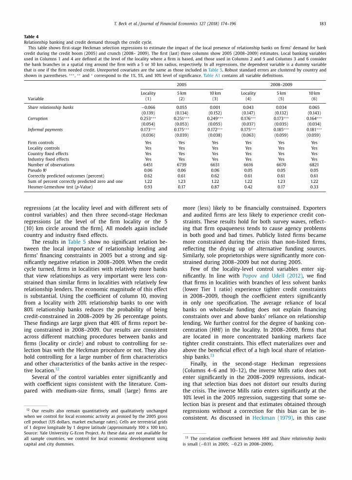
As expected, Corruption and Informal Payments are posi-

tively and significantly correlated with a firm’s demand for

credit. Importantly, we find no relation, neither in 2005

nor in 20 08–20 09, between our variable measuring the

local presence of relationship banks and the demand for

credit [either at the level of the firm locality or at the 5

(10) km circle around the firm]. This gives us confidence

that Share relationship banks is not endogenous to local de-

mand conditions and, hence, a good candidate to subse-

quently identify shifts in the supply of credit.

At the bottom of Table 4 , we provide three goodness-of-

fit measures and the pseudo R ², which perhaps is not the

most appropriate measure when dealing with a binary de-

pendent variable. “Correctly predicted outcomes (percent)”

and “Sum of percent correctly predicted zero and one”

provide information on the correctly predicted outcomes.

We predict 61% to 62% of all outcomes correctly. Accord-

ing to McIntosh and Dorfman (1992) , the sum of the frac-

tion of zeroes correctly predicted plus the fraction of ones

correctly predicted should exceed unity if the prediction

method is of value. In our case the sum of these fractions

is 1.22 or 1.23, which is reassuring. The third measure is

the Hosmer and Lemeshow (2013) test statistic [“Hosmer-

Lemeshow test ( p -Value)”]. This test investigates whether

the fitted model is correct across the model population,

i.e., whether the observed events match expected events

in different subgroups of the population. Following stan-

dard practice, we employ ten groups of equal size. The test

consistently reveals that we cannot reject the null hypoth-

esis that the fitted model is correct. 11

Next, in Table 5 , we present regression specifications

in line with Eq. (1) to estimate the association between

the local presence of relationship banks and firms’ access

to credit. We first show results for 2005 (the time of the

credit boom) and then for 20 08–20 09 (when the credit

cycle had turned). For each period, we present three probit

11 The p -Values of the Hosmer-Lemeshow tests vary considerably across

specifications, reflecting the sensitivity of this test to changes in specifi-

cation or sample size. As an additional check, we reran the specifications

in Table 4 while using either nine or 11 population groups instead of the

standard ten. In all cases, the calculated p -Value remains larger than 0.05

so that we cannot reject the null of a good fit.

T. Beck et al. / Journal of Financial Economics 127 (2018) 174–196 183

Table 4

Relationship banking and credit demand through the credit cycle.

This table shows first-stage Heckman selection regressions to estimate the impact of the local presence of relationship banks on firms‘ demand for bank

credit during the credit boom (2005) and crunch (2008– 2009). The first (last) three columns show 2005 (2008–2009) estimates. Local banking variables

used in Columns 1 and 4 are defined at the level of the locality where a firm is based, and those used in Columns 2 and 5 and Columns 3 and 6 consider

the bank branches in a spatial ring around the firm with a 5 or 10 km radius, respectively. In all regressions, the dependent variable is a dummy variable

that is one if the firm needed credit. Unreported covariates are the same as those included in Table 5 . Robust standard errors are clustered by country and

shown in parentheses. ∗∗∗ , ∗∗ and ∗ correspond to the 1%, 5%, and 10% level of significance. Table A1 contains all variable definitions.

2005 20 08–20 09

Locality 5 km 10 km Locality 5 km 10 km

Variable (1) (2) (3) (4) (5) (6)

Share relationship banks −0.066 0.055 0.001 0.043 0.034 0.065

(0.139) (0.134) (0.152) (0.147) (0.132) (0.143)

Corruption 0.253 ∗∗∗ 0.251 ∗∗∗ 0.249 ∗∗∗ 0.176 ∗∗∗ 0.173 ∗∗∗ 0.164 ∗∗∗

(0.054) (0.053) (0.055) (0.037) (0.035) (0.034)

Informal payments 0.173 ∗∗∗ 0.175 ∗∗∗ 0.172 ∗∗∗ 0.175 ∗∗∗ 0.185 ∗∗∗ 0.181 ∗∗∗

(0.036) (0.039) (0.038) (0.063) (0.059) (0.059)

Firm controls Yes Yes Yes Yes Yes Yes

Locality controls Yes Yes Yes Yes Yes Yes

Country fixed effects Yes Yes Yes Yes Yes Yes

Industry fixed effects Yes Yes Yes Yes Yes Yes

Number of observations 6451 6739 6631 6616 6670 6821

Pseudo R ² 0.06 0.06 0.06 0.05 0.05 0.05

Correctly predicted outcomes (percent) 0.62 0.61 0.62 0.61 0.61 0.61

Sum of percent correctly predicted zero and one 1.22 1.23 1.22 1.22 1.23 1.22

Hosmer-Lemeshow test ( p -Value) 0.93 0.17 0.87 0.42 0.17 0.33

regressions (at the locality level and with different sets of

control variables) and then three second-stage Heckman

regressions [at the level of the firm locality or the 5

(10) km circle around the firm]. All models again include

country and industry fixed effects.

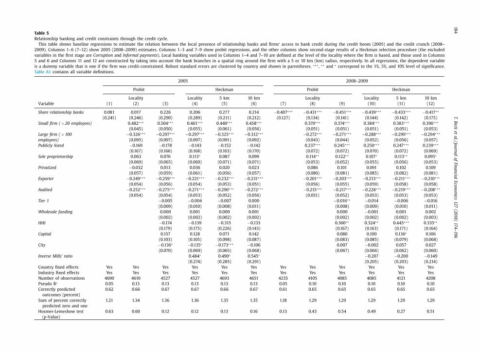
The results in Table 5 show no significant relation be-

tween the local importance of relationship lending and

firms’ financing constraints in 2005 but a strong and sig-

nificantly negative relation in 20 08–20 09. When the credit

cycle turned, firms in localities with relatively more banks

that view relationships as very important were less con-

strained than similar firms in localities with relatively few

relationship lenders. The economic magnitude of this effect

is substantial. Using the coefficient of column 10, moving

from a locality with 20% relationship banks to one with

80% relationship banks reduces the probability of being

credit-constrained in 20 08–20 09 by 26 percentage points.

These findings are large given that 40% of firms report be-

ing constrained in 20 08–20 09. Our results are consistent

across different matching procedures between banks and

firms (locality or circle) and robust to controlling for se-

lection bias with the Heckman procedure or not. They also

hold controlling for a large number of firm characteristics

and other characteristics of the banks active in the respec-

tive location. 12

Several of the control variables enter significantly and

with coefficient signs consistent with the literature. Com-

pared with medium-size firms, small (large) firms are

12 Our results also remain quantitatively and qualitatively unchanged

when we control for local economic activity as proxied by the 2005 gross

cell product (US dollars, market exchange rates). Cells are terrestrial grids

of 1 degree longitude by 1 degree latitude (approximately 100 x 100 km).

Source: Yale University G-Econ Project. As these data are not available for

all sample countries, we control for local economic development using

capital and city dummies.

more (less) likely to be financially constrained. Exporters

and audited firms are less likely to experience credit con-

straints. These results hold for both survey waves, reflect-

ing that firm opaqueness tends to cause agency problems

in both good and bad times. Publicly listed firms became

more constrained during the crisis than non-listed firms,

reflecting the drying up of alternative funding sources.

Similarly, sole proprietorships were significantly more con-

strained during 20 08–20 09 but not during 2005.

Few of the locality-level control variables enter sig-

nificantly. In line with Popov and Udell (2012) , we find

that firms in localities with branches of less solvent banks

(lower Tier 1 ratio) experience tighter credit constraints

in 20 08–20 09, though the coefficient enters significantly

in only one specification. The average reliance of local

banks on wholesale funding does not explain financing

constraints over and above banks’ reliance on relationship

lending. We further control for the degree of banking con-

centration ( HHI ) in the locality. In 20 08–20 09, firms that

are located in more concentrated banking markets face

tighter credit constraints. This effect materializes over and

above the beneficial effect of a high local share of relation-

ship banks. 13

Finally, in the second-stage Heckman regressions

(Columns 4–6 and 10–12), the inverse Mills ratio does not

enter significantly in the 20 08–20 09 regressions, indicat-

ing that selection bias does not distort our results during

the crisis. The inverse Mills ratio enters significantly at the

10% level in the 2005 regression, suggesting that some se-

lection bias is present and that estimates obtained through

regressions without a correction for this bias can be in-

consistent. As discussed in Heckman (1979) , in this case

13 The correlation coefficient between HHI and Share relationship banks

is small ( −0.11 in 2005; −0.23 in 2008–2009).

18

4

T. B

eck et

al. / Jo

urn

al o

f Fin

an

cial E

con

om

ics 1

27 (2

018

) 17

4–

196

Table 5

Relationship banking and credit constraints through the credit cycle.

This table shows baseline regressions to estimate the relation between the local presence of relationship banks and firms‘ access to bank credit during the credit boom (2005) and the credit crunch (2008–

2009). Columns 1–6 (7–12) show 2005 (2008–2009) estimates. Columns 1–3 and 7–9 show probit regressions, and the other columns show second-stage results of a Heckman selection procedure (the excluded

variables in the first stage are Corruption and Informal payments ). Local banking variables used in Columns 1–4 and 7–10 are defined at the level of the locality where the firm is based, and those used in Columns

5 and 6 and Columns 11 and 12 are constructed by taking into account the bank branches in a spatial ring around the firm with a 5 or 10 km (km) radius, respectively. In all regressions, the dependent variable

is a dummy variable that is one if the firm was credit-constrained. Robust standard errors are clustered by country and shown in parentheses. ∗∗∗ , ∗∗ and ∗ correspond to the 1%, 5%, and 10% level of significance.

Table A1 contains all variable definitions.

2005 20 08–20 09

Probit Heckman Probit Heckman

Locality Locality 5 km 10 km Locality Locality 5 km 10 km

Variable (1) (2) (3) (4) (5) (6) (7) (8) (9) (10) (11) (12)

Share relationship banks 0.081 0.017 0.226 0.206 0.277 0.214 −0.407 ∗∗∗ −0.431 ∗∗∗ −0.451 ∗∗∗ −0.439 ∗∗∗ −0.433 ∗∗∗ −0.417 ∗∗

(0.241) (0.246) (0.290) (0.289) (0.211) (0.212) (0.127) (0.134) (0.141) (0.144) (0.142) (0.175)

Small firm ( < 20 employees) 0.482 ∗∗∗ 0.504 ∗∗∗ 0.461 ∗∗∗ 0.440 ∗∗∗ 0.458 ∗∗∗ 0.370 ∗∗∗ 0.374 ∗∗∗ 0.384 ∗∗∗ 0.383 ∗∗∗ 0.396 ∗∗∗

(0.045) (0.050) (0.055) (0.061) (0.056) (0.051) (0.051) (0.051) (0.051) (0.053)

Large firm ( > 100

employees)

−0.326 ∗∗∗ −0.297 ∗∗∗ −0.297 ∗∗∗ −0.325 ∗∗∗ −0.312 ∗∗∗ −0.272 ∗∗∗ −0.271 ∗∗∗ −0.288 ∗∗∗ −0.299 ∗∗∗ −0.294 ∗∗∗

(0.095) (0.097) (0.097) (0.091) (0.092) (0.043) (0.044) (0.052) (0.056) (0.057)

Publicly listed −0.169 −0.178 −0.143 −0.152 −0.142 0.237 ∗∗∗ 0.245 ∗∗∗ 0.250 ∗∗∗ 0.247 ∗∗∗ 0.239 ∗∗∗

(0.167) (0.166) (0.168) (0.163) (0.170) (0.072) (0.072) (0.070) (0.072) (0.069)

Sole proprietorship 0.063 0.076 0.113 ∗ 0.087 0.099 0.114 ∗∗ 0.122 ∗∗ 0.107 ∗ 0.113 ∗∗ 0.095 ∗

(0.069) (0.065) (0.069) (0.071) (0.071) (0.053) (0.052) (0.055) (0.056) (0.053)

Privatized −0.032 0.013 0.036 0.020 0.023 0.086 0.101 0.091 0.102 0.109

(0.057) (0.059) (0.061) (0.056) (0.057) (0.080) (0.081) (0.085) (0.082) (0.081)

Exporter −0.249 ∗∗∗ −0.259 ∗∗∗ −0.221 ∗∗∗ −0.232 ∗∗∗ −0.231 ∗∗∗ −0.201 ∗∗∗ −0.203 ∗∗∗ −0.213 ∗∗∗ −0.211 ∗∗∗ −0.210 ∗∗∗

(0.054) (0.056) (0.054) (0.053) (0.051) (0.056) (0.055) (0.059) (0.058) (0.058)

Audited −0.252 ∗∗∗ −0.275 ∗∗∗ −0.271 ∗∗∗ −0.290 ∗∗∗ −0.272 ∗∗∗ −0.215 ∗∗∗ −0.217 ∗∗∗ −0.228 ∗∗∗ −0.219 ∗∗∗ −0.208 ∗∗∗

(0.054) (0.054) (0.053) (0.052) (0.056) (0.051) (0.052) (0.053) (0.053) (0.053)

Tier 1 −0.005 −0.004 −0.007 0.0 0 0 −0.016 ∗∗ −0.014 −0.006 −0.016

(0.009) (0.010) (0.008) (0.011) (0.008) (0.009) (0.010) (0.011)

Wholesale funding 0.0 0 0 0.001 0.0 0 0 0.001 0.0 0 0 −0.001 0.001 0.002

(0.002) (0.002) (0.002) (0.002) (0.002) (0.002) (0.002) (0.003)

HHI −0.174 −0.139 −0.315 −0.133 0.360 ∗∗ 0.324 ∗∗ 0.445 ∗∗∗ 0.335 ∗∗

(0.179) (0.175) (0.226) (0.143) (0.167) (0.163) (0.171) (0.164)

Capital 0.157 0.128 0.071 0.142 0.080 0.100 0.136 ∗ 0.106

(0.103) (0.105) (0.098) (0.087) (0.083) (0.085) (0.079) (0.068)

City −0.136 ∗ −0.135 ∗ −0.173 ∗∗∗ −0.106 0.007 −0.002 0.057 0.027

(0.070) (0.069) (0.065) (0.068) (0.067) (0.066) (0.062) (0.060)

Inverse Mills‘ ratio 0.484 ∗ 0.490 ∗ 0.545 ∗ −0.207 −0.200 −0.149

(0.274) (0.285) (0.291) (0.205) (0.203) (0.214)

Country fixed effects Yes Yes Yes Yes Yes Yes Yes Yes Yes Yes Yes Yes

Industry fixed effects Yes Yes Yes Yes Yes Yes Yes Yes Yes Yes Yes Yes

Number of observations 4690 4610 4527 4527 4693 4651 4235 4105 4085 4085 4121 4208

Pseudo R ² 0.05 0.13 0.13 0.13 0.13 0.13 0.05 0.10 0.10 0.10 0.10 0.10

Correctly predicted

outcomes (percent)

0.62 0.66 0.67 0.67 0.66 0.67 0.61 0.65 0.65 0.65 0.65 0.65

Sum of percent correctly

predicted zero and one

1.21 1.34 1.36 1.36 1.35 1.35 1.18 1.29 1.29 1.29 1.29 1.29

Hosmer-Lemeshow test

( p -Value)

0.63 0.60 0.12 0.12 0.13 0.16 0.13 0.43 0.54 0.49 0.27 0.51

T. Beck et al. / Journal of Financial Economics 127 (2018) 174–196 185

the standard errors obtained in the second step are un-

derstated and significance levels are therefore overstated.

This reinforces our finding of the absence of a significant

relation between the local presence of relationship bank-

ing and firms’ credit constraints in 2005. The insignificance

of the inverse Mills ratio in 20 08–20 09 and the positive,

though only borderline significant, inverse Mills ratio in

2005 also suggest that, in 2005, a firm with average sam-

ple characteristics that selects into a need for credit has

a somewhat higher probability of being credit-constrained

than a firm that is drawn at random from the entire pop-

ulation with the average set of characteristics and that, in

20 08–20 09, firms in need of credit were less special and

closer to the typical firm in the population at large.

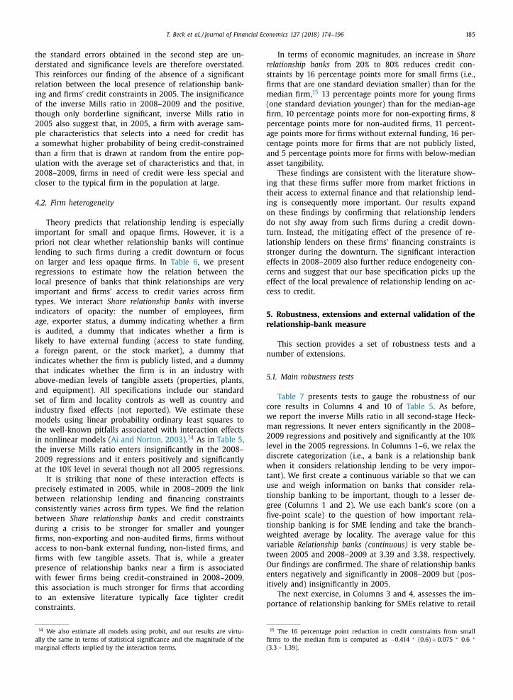
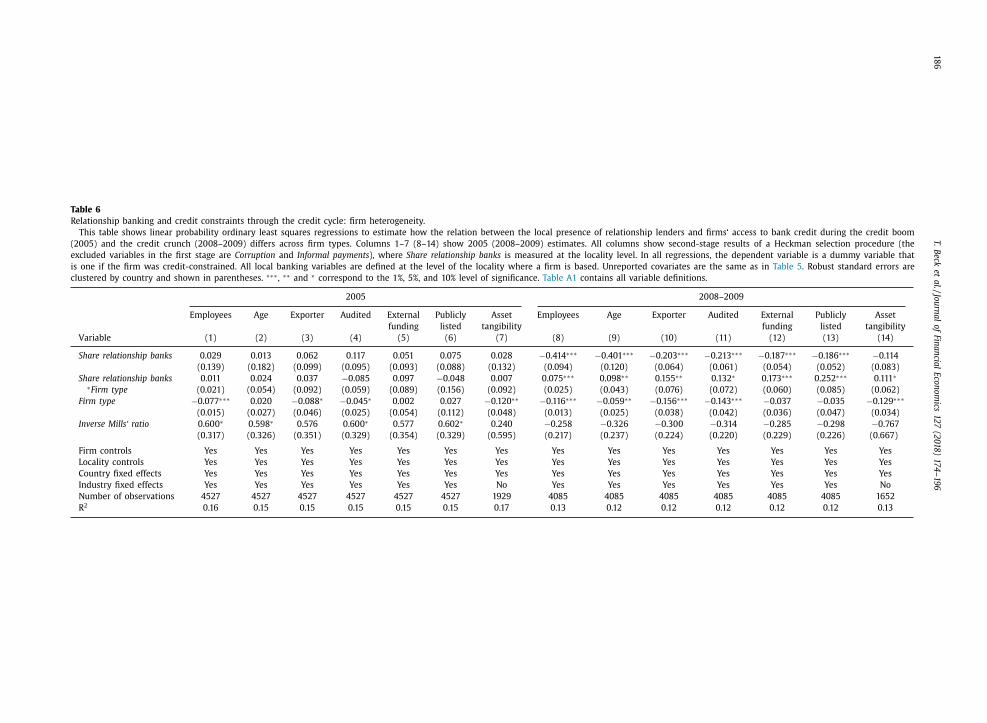
4.2. Firm heterogeneity

Theory predicts that relationship lending is especially

important for small and opaque firms. However, it is a

priori not clear whether relationship banks will continue

lending to such firms during a credit downturn or focus

on larger and less opaque firms. In Table 6 , we present

regressions to estimate how the relation between the

local presence of banks that think relationships are very

important and firms’ access to credit varies across firm

types. We interact Share relationship banks with inverse

indicators of opacity: the number of employees, firm

age, exporter status, a dummy indicating whether a firm

is audited, a dummy that indicates whether a firm is

likely to have external funding (access to state funding,

a foreign parent, or the stock market), a dummy that

indicates whether the firm is publicly listed, and a dummy

that indicates whether the firm is in an industry with

above-median levels of tangible assets (properties, plants,

and equipment). All specifications include our standard

set of firm and locality controls as well as country and

industry fixed effects (not reported). We estimate these

models using linear probability ordinary least squares to

the well-known pitfalls associated with interaction effects

in nonlinear models ( Ai and Norton, 2003 ). 14 As in Table 5 ,

the inverse Mills ratio enters insignificantly in the 2008–

2009 regressions and it enters positively and significantly

at the 10% level in several though not all 2005 regressions.

It is striking that none of these interaction effects is

precisely estimated in 2005, while in 20 08–20 09 the link

between relationship lending and financing constraints

consistently varies across firm types. We find the relation

between Share relationship banks and credit constraints

during a crisis to be stronger for smaller and younger

firms, non-exporting and non-audited firms, firms without

access to non-bank external funding, non-listed firms, and

firms with few tangible assets. That is, while a greater

presence of relationship banks near a firm is associated

with fewer firms being credit-constrained in 20 08–20 09,

this association is much stronger for firms that according

to an extensive literature typically face tighter credit

constraints.

14 We also estimate all models using probit, and our results are virtu-

ally the same in terms of statistical significance and the magnitude of the

marginal effects implied by the interaction terms.

In terms of economic magnitudes, an increase in Share

relationship banks from 20% to 80% reduces credit con-

straints by 16 percentage points more for small firms (i.e.,

firms that are one standard deviation smaller) than for the

median firm, 15 13 percentage points more for young firms

(one standard deviation younger) than for the median-age

firm, 10 percentage points more for non-exporting firms, 8

percentage points more for non-audited firms, 11 percent-

age points more for firms without external funding, 16 per-

centage points more for firms that are not publicly listed,

and 5 percentage points more for firms with below-median

asset tangibility.

These findings are consistent with the literature show-

ing that these firms suffer more from market frictions in

their access to external finance and that relationship lend-

ing is consequently more important. Our results expand

on these findings by confirming that relationship lenders

do not shy away from such firms during a credit down-

turn. Instead, the mitigating effect of the presence of re-

lationship lenders on these firms’ financing constraints is

stronger during the downturn. The significant interaction

effects in 20 08–20 09 also further reduce endogeneity con-

cerns and suggest that our base specification picks up the

effect of the local prevalence of relationship lending on ac-

cess to credit.

5. Robustness, extensions and external validation of the

relationship-bank measure

This section provides a set of robustness tests and a

number of extensions.

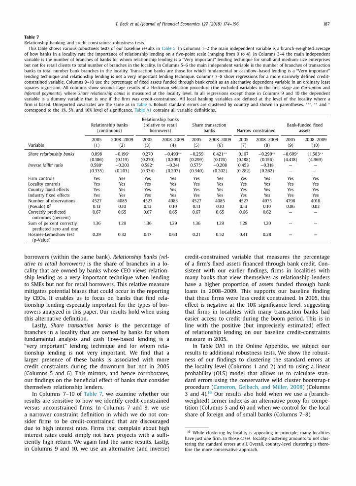
5.1. Main robustness tests

Table 7 presents tests to gauge the robustness of our

core results in Columns 4 and 10 of Table 5 . As before,

we report the inverse Mills ratio in all second-stage Heck-

man regressions. It never enters significantly in the 2008–

2009 regressions and positively and significantly at the 10%

level in the 2005 regressions. In Columns 1–6, we relax the

discrete categorization (i.e., a bank is a relationship bank

when it considers relationship lending to be very impor-

tant). We first create a continuous variable so that we can

use and weigh information on banks that consider rela-

tionship banking to be important, though to a lesser de-

gree (Columns 1 and 2). We use each bank’s score (on a

five-point scale) to the question of how important rela-

tionship banking is for SME lending and take the branch-

weighted average by locality. The average value for this

variable Relationship banks (continuous) is very stable be-

tween 2005 and 2008–2009 at 3.39 and 3.38, respectively.

Our findings are confirmed. The share of relationship banks

enters negatively and significantly in 20 08–20 09 but (pos-

itively and) insignificantly in 2005.

The next exercise, in Columns 3 and 4, assesses the im-

portance of relationship banking for SMEs relative to retail

15 The 16 percentage point reduction in credit constraints from small

firms to the median firm is computed as −0.414 ∗ (0.6) + 0.075 ∗ 0.6 ∗

(3.3 - 1.39).

18

6

T. B

eck et

al. / Jo

urn

al o

f Fin

an

cial E

con

om

ics 1

27 (2

018

) 17

4–

196

Table 6

Relationship banking and cred it constraints through the credit cycle: firm heterogeneity.

This table shows linear probability ordinary least squares regressions to estimate how the relation between the local presence of relationship lenders and firms‘ access to bank credit during the credit boom

(2005) and the credit crunch (20 08–20 09) differs across firm types. Columns 1–7 (8–14) show 20 05 (20 08–20 09) estimates. All columns show second-stage results of a Heckman selection procedure (the

excluded variables in the first stage are Corruption and Informal payments ), where Share relationship banks is measured at the locality level. In all regressions, the dependent variable is a dummy variable that

is one if the firm was credit-constrained. All local banking variables are defined at the level of the locality where a firm is based. Unreported covariates are the same as in Table 5 . Robust standard errors are

clustered by country and shown in parentheses. ∗∗∗ , ∗∗ and ∗ correspond to the 1%, 5%, and 10% level of significance. Table A1 contains all variable definitions.

2005 20 08–20 09

Employees Age Exporter Audited External Publicly Asset Employees Age Exporter Audited External Publicly Asset

funding listed tangibility funding listed tangibility

Variable (1) (2) (3) (4) (5) (6) (7) (8) (9) (10) (11) (12) (13) (14)

Share relationship banks 0.029 0.013 0.062 0.117 0.051 0.075 0.028 −0.414 ∗∗∗ −0.401 ∗∗∗ −0.203 ∗∗∗ −0.213 ∗∗∗ −0.187 ∗∗∗ −0.186 ∗∗∗ −0.114

(0.139) (0.182) (0.099) (0.095) (0.093) (0.088) (0.132) (0.094) (0.120) (0.064) (0.061) (0.054) (0.052) (0.083)

Share relationship banks 0.011 0.024 0.037 −0.085 0.097 −0.048 0.007 0.075 ∗∗∗ 0.098 ∗∗ 0.155 ∗∗ 0.132 ∗ 0.173 ∗∗∗ 0.252 ∗∗∗ 0.111 ∗∗Firm type (0.021) (0.054) (0.092) (0.059) (0.089) (0.156) (0.092) (0.025) (0.043) (0.076) (0.072) (0.060) (0.085) (0.062)

Firm type −0.077 ∗∗∗ 0.020 −0.088 ∗ −0.045 ∗ 0.002 0.027 −0.120 ∗∗ −0.116 ∗∗∗ −0.059 ∗∗ −0.156 ∗∗∗ −0.143 ∗∗∗ −0.037 −0.035 −0.129 ∗∗∗

(0.015) (0.027) (0.046) (0.025) (0.054) (0.112) (0.048) (0.013) (0.025) (0.038) (0.042) (0.036) (0.047) (0.034)

Inverse Mills‘ ratio 0.600 ∗ 0.598 ∗ 0.576 0.600 ∗ 0.577 0.602 ∗ 0.240 −0.258 −0.326 −0.300 −0.314 −0.285 −0.298 −0.767

(0.317) (0.326) (0.351) (0.329) (0.354) (0.329) (0.595) (0.217) (0.237) (0.224) (0.220) (0.229) (0.226) (0.667)

Firm controls Yes Yes Yes Yes Yes Yes Yes Yes Yes Yes Yes Yes Yes Yes

Locality controls Yes Yes Yes Yes Yes Yes Yes Yes Yes Yes Yes Yes Yes Yes

Country fixed effects Yes Yes Yes Yes Yes Yes Yes Yes Yes Yes Yes Yes Yes Yes

Industry fixed effects Yes Yes Yes Yes Yes Yes No Yes Yes Yes Yes Yes Yes No

Number of observations 4527 4527 4527 4527 4527 4527 1929 4085 4085 4085 4085 4085 4085 1652

R 2 0.16 0.15 0.15 0.15 0.15 0.15 0.17 0.13 0.12 0.12 0.12 0.12 0.12 0.13

T. Beck et al. / Journal of Financial Economics 127 (2018) 174–196 187

Table 7

Relationship banking and credit constraints: robustness tests.

This table shows various robustness tests of our baseline results in Table 5 . In Columns 1–2 the main independent variable is a branch-weighted average

of how banks in a locality rate the importance of relationship lending on a five-point scale (ranging from 0 to 4). In Columns 3–4 the main independent

variable is the number of branches of banks for whom relationship lending is a “Very important” lending technique for small and medium-size enterprises

but not for retail clients to total number of branches in the locality. In Columns 5–6 the main independent variable is the number of branches of transaction

banks to total number bank branches in the locality. Transaction banks are those for which fundamental or cashflow–based lending is a “Very important”

lending technique and relationship lending is not a very important lending technique. Columns 7–8 show regressions for a more narrowly defined credit-

constrained variable. Columns 9–10 use the percentage of fixed assets funded through bank credit as an alternative dependent variable in an ordinary least

squares regression. All columns show second-stage results of a Heckman selection procedure (the excluded variables in the first stage are Corruption and

Informal payments ), where Share relationship banks is measured at the locality level. In all regressions except those in Columns 9 and 10 the dependent

variable is a dummy variable that is one if the firm was credit-constrained. All local banking variables are defined at the level of the locality where a

firm is based. Unreported covariates are the same as in Table 5 . Robust standard errors are clustered by country and shown in parentheses. ∗∗∗ , ∗∗ and ∗

correspond to the 1%, 5%, and 10% level of significance. Table A1 contains all variable definitions.

Relationship banks

(continuous)

Relationship banks

(relative to retail

borrowers)

Share transaction

banks Narrow constrained

Bank-funded fixed

assets

2005 20 08–20 09 2005 20 08–20 09 2005 20 08–20 09 2005 20 08–20 09 2005 20 08–20 09

Variable (1) (2) (3) (4) (5) (6) (7) (8) (9) (10)

Share relationship banks 0.098 −0.196 ∗ 0.270 −0.493 ∗∗ −0.259 0.421 ∗∗ 0.107 −0.299 ∗∗ −8.609 ∗ 11.583 ∗∗

(0.186) (0.119) (0.270) (0.209) (0.299) (0.176) (0.188) (0.156) (4.418) (4.969)

Inverse Mills‘ ratio 0.580 ∗ −0.203 0.582 ∗ −0.241 0.575 ∗ −0.208 0.453 −0.318 — —

(0.335) (0.203) (0.334) (0.207) (0.340) (0.202) (0.282) (0.262) — —

Firm controls Yes Yes Yes Yes Yes Yes Yes Yes Yes Yes

Locality controls Yes Yes Yes Yes Yes Yes Yes Yes Yes Yes

Country fixed effects Yes Yes Yes Yes Yes Yes Yes Yes Yes Yes

Industry fixed effects Yes Yes Yes Yes Yes Yes Yes Yes Yes Yes

Number of observations 4527 4085 4527 4083 4527 4085 4527 4075 4798 4018

(Pseudo) R 2 0.13 0.10 0.13 0.10 0.13 0.10 0.13 0.10 0.06 0.03

Correctly predicted

outcomes (percent)

0.67 0.65 0.67 0.65 0.67 0.65 0.66 0.62 — —

Sum of percent correctly

predicted zero and one

1.36 1.29 1.36 1.29 1.36 1.29 1.28 1.20 — —

Hosmer-Lemeshow test

( p -Value)

0.29 0.32 0.17 0.63 0.21 0.52 0.41 0.28 — —

16 While clustering by locality is appealing in principle, many localities

have just one firm. In those cases, locality clustering amounts to not clus-

tering the standard errors at all. Overall, country-level clustering is there-

fore the more conservative approach.

borrowers (within the same bank). Relationship banks (rel-

ative to retail borrowers) is the share of branches in a lo-

cality that are owned by banks whose CEO views relation-

ship lending as a very important technique when lending

to SMEs but not for retail borrowers. This relative measure

mitigates potential biases that could occur in the reporting

by CEOs. It enables us to focus on banks that find rela-

tionship lending especially important for the types of bor-

rowers analyzed in this paper. Our results hold when using

this alternative definition.

Lastly, Share transaction banks is the percentage of

branches in a locality that are owned by banks for whom

fundamental analysis and cash flow-based lending is a

“very important” lending technique and for whom rela-

tionship lending is not very important. We find that a

larger presence of these banks is associated with more

credit constraints during the downturn but not in 2005

(Columns 5 and 6). This mirrors, and hence corroborates,

our findings on the beneficial effect of banks that consider

themselves relationship lenders.

In Columns 7–10 of Table 7 , we examine whether our

results are sensitive to how we identify credit-constrained

versus unconstrained firms. In Columns 7 and 8, we use

a narrower constraint definition in which we do not con-

sider firms to be credit-constrained that are discouraged

due to high interest rates. Firms that complain about high

interest rates could simply not have projects with a suffi-

ciently high return. We again find the same results. Lastly,

in Columns 9 and 10, we use an alternative (and inverse)

credit-constrained variable that measures the percentage

of a firm’s fixed assets financed through bank credit. Con-

sistent with our earlier findings, firms in localities with

many banks that view themselves as relationship lenders

have a higher proportion of assets funded through bank

loans in 20 08–20 09. This supports our baseline finding

that these firms were less credit constrained. In 2005, this

effect is negative at the 10% significance level, suggesting

that firms in localities with many transaction banks had

easier access to credit during the boom period. This is in

line with the positive (but imprecisely estimated) effect

of relationship lending on our baseline credit-constraints

measure in 2005.

In Table OA1 in the Online Appendix, we subject our

results to additional robustness tests. We show the robust-

ness of our findings to clustering the standard errors at

the locality level (Columns 1 and 2) and to using a linear

probability (OLS) model that allows us to calculate stan-

dard errors using the conservative wild cluster bootstrap-t

procedure ( Cameron, Gelbach, and Miller, 2008 ) (Columns

3 and 4). 16 Our results also hold when we use a (branch-

weighted) Lerner index as an alternative proxy for compe-

tition (Columns 5 and 6) and when we control for the local

share of foreign and of small banks (Columns 7–8).

188 T. Beck et al. / Journal of Financial Economics 127 (2018) 174–196

19 We also follow Altonji, Elder, and Taber (2005) and Bellows and

Miguel (2009) to assess omitted variable bias by gauging the coefficient

stability across specifications. We calculate the ratio between the coeffi-

cient in the regression including controls (numerator) and the difference

Pooling the 2005 and 20 08–20 09 observations and in-

cluding an interaction term between the share of relation-

ship banks and a 20 08–20 09 dummy yields an insignif-

icant coefficient on the share of relationship banks and

a statistically significant negative coefficient for the in-

teraction term, thus confirming that the role of the lo-

cal presence of relationship banks is limited to the down-

turn (Column 9). Dropping the largest country in our sam-

ple, Ukraine, shows that our findings are not driven by

this single country (Columns 10 and 11). We also confirm

our findings when excluding banks that experienced an

ownership change during our sample period when com-

puting Share relationship banks ; that is, arguably, for this

group of banks, lending techniques have been most stable

over time (Columns 12 and 13). Finally, excluding multi-

establishment firms (123 firms in 2005; 164 firms in 2008–

2009), which can be subject to the banking environment in

several localities, confirms our findings (Columns 14 and

15). 17

5.2. Addressing endogeneity

We next assess whether our findings could be driven by

endogeneity. The insignificant coefficient of Share relation-

ship banks in the loan-demand regressions of Table 4 is re-

assuring. It suggests that relationship banks did not select

into localities with a higher demand for external finance.

However, we cannot exclude the possibility that new firms

selected into localities with a higher share of relationship

banks to secure funding throughout the credit cycle. We

therefore re-run our regressions dropping firms that were

established either less than five years ago or less than 12

years ago (the median firm age in our sample). Columns

1–4 of Table OA2 in the Online Appendix confirm our find-

ings. Next, the regressions in Columns 5–8 show the ro-

bustness of our results by replacing the current branch-

weighted share of relationship banks with the historical

branch-weighted share of these banks in either 1995 or

20 0 0. Using the lagged value of relationship banks in a

locality reduces the risk that our findings are driven by

banks’ viewing themselves as relationship lenders entering

localities to serve firms with a higher need for external fi-

nance. This confirms our findings. 18

To further mitigate concerns, we ran an (unreported)

locality-level regression of the Share relationship banks in

2008 on characteristics of the local firm population as well

as country and industry fixed effects. If the presence of

relationship banks were driven by the composition of the

business sector in a locality, then we should find signifi-

cant correlations between firm characteristics averaged at

the locality level and the share of relationship banks. Yet,

we do not find any significant relation between, on the one

hand, the share of small firms, large firms, sole proprietor-

17 As in Table 5 , the inverse Mills ratio enters insignificantly in the

20 08–20 09 regressions and positively and significantly at the 10% level in

the 2005 regressions. In Column 9, where we use the combined sample,

it does not enter significantly. 18 As before, we find an insignificant inverse Mills ratio in the 2008–

2009 regression and a positive and significant at the 10% level inverse

Mills ratio in the 2005 regressions.

ships, privatized firms, exporters, or audited firms and, on

the other hand, the share of relationship banks. We find

only one marginally significant positive association, at the

10% level, between the share of publicly listed firms and

the share of relationship banks. An F -test for the joint sig-

nificance of these local firm characteristics cannot reject

the null of no systematic relation between firm character-

istics and the presence of relationship banks ( p -Value: .25).

We conclude that the presence of banks’ viewing them-

selves as relationship banks in a locality is unrelated to a

large set of observable firm characteristics. 19

5.3. Are bank CEOs’ views in line with actual indicators of

relationship lending?

Our measure of relationship lenders is unique com-

pared with the existing literature as it is based on a sur-

vey of bank CEOs. In light of possible biases due to per-

ceptions of individual CEOs or cross-country cultural dif-

ferences, we look for external validation of this measure

by employing information from the Armenian Credit Re-

porting Agency. This credit registry contains information

on all credit products, i.e., there are no minimum loan size

reporting restrictions, sold to firms between January 2009

and June 2013 (more than 40 thousand contracts). Slightly

over half of these are standard loans and the remainder are

credit lines, factoring, leasing, guarantees, letters of credit,

overdrafts, and repurchase agreements. Sch ӓfer (2016) pro-

vides more details on these data.

Armenia is one of the countries in our sample and is

well covered by the BEPS II survey. Seventeen out of 19

Armenian banks participated in the survey and can there-

fore be classified as a relationship or transaction bank. The

structure of the Armenian banking system is also represen-

tative of our country sample. According to our definition,

59% (41%) of Armenian banks are relationship (transaction)

banks. In our full country sample, these numbers are 58%

(42%). Similarly, while 70% of all Armenian banks are for-

eign owned, this number is 65% in the full country sample.

Finally, of all foreign-owned Armenian banks 64% are clas-

sified as a relationship bank. In the full country sample,

this share is also 64%.

We use the detailed registry information on Armenian

relationship and transaction banks to test whether any ob-

servable differences between both bank types are in line

with the previous literature on relationship lending. If so,

this would provide strong support for our survey-based

bank classification and the empirical results based on that

between this coefficient and one derived from a regression without co-

variates (denominator). This ratio shows how strong the covariance be-

tween the unobserved factors explaining credit constraints and the share

of relationship banks needs to be, relative to the covariance between ob-

servable factors and the share of relationship banks, to explain away our

effect. This ratio is 142.7 and 41.9 for the specifications in Columns 9 (pro-

bit) and 10 (Heckman) of Table 5 . These high ratios indicate that the coef-

ficient for Share relationship banks is remarkably stable when we add co-

variates. Therefore, unobserved heterogeneity is unlikely to explain away

the protective role of local relationship lending that we show.

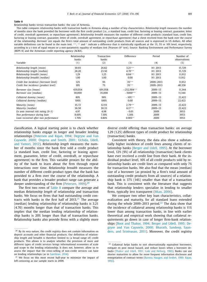
T. Beck et al. / Journal of Financial Economics 127 (2018) 174–196 189

Table 8

Relationship banks versus transaction banks: the case of Armenia.

This table compares relationship banks with transaction banks in Armenia along a number of key characteristics. Relationship length measures the number

of months since the bank provided the borrower with the first credit product (i.e., a standard loan, credit line, factoring or leasing contract, guarantee, letter

of credit, overdraft agreement, or repurchase agreement). Relationship breadth measures the number of different credit products (standard loan, credit line,

factoring or leasing contract, guarantee, letter of credit, overdraft agreement, or repurchase agreement) that a client received from the bank over the course

of the relationship. Borrower size equals the firm‘s total amount of outstanding credit products from all sources and is expressed in US dollars. All other

variable definitions can be found in the main text. ∗∗∗ , ∗∗ and ∗ indicate a difference that is statistically significant at the 1%, 5% or 10% level, respectively,

according to a t -test of equal means or a non-parametric equality of medians test (Pearson ch 2 test). Source: Banking Environment and Performance Survey

(BEPS II) and the Armenian credit reporting agency (ACRA).

Relationship Transaction Difference Period Number of

banks banks observations

Variable (1) (2) (3) (4) (5)

Relationship length (mean) 30.03 26.82 3.21 ∗∗∗ H1 2013 15,729

Relationship length (median) 28.20 23.50 4.70 ∗∗∗ H1 2013 15,729

Relationship breadth (mean) 1.29 1.25 0.04 ∗∗∗ H1 2013 11,912

Relationship breadth (median) 1.00 1.00 0.00 H1 2013 11,912

Credit line incidence (borrower level) 12% 9% 3% ∗∗∗ 2009–2013 11,912

Credit line incidence (product level) 10% 7% 3% ∗∗∗ 2009–2013 40,358

Borrower size (mean) 439,054 691,958 −252,904 ∗∗∗ 2009–13 11,344

Borrower size (median) 30,0 0 0 35,0 0 0 −50 0 0 ∗∗∗ 2009–13 11,344

Collateral dummy (mean) 80% 90% −10% ∗∗∗ 2009–13 22,422

Collateral dummy (median) 100% 100% 0.00 2009–13 22,422

Maturity (mean) 35.72 32.93 2.79 ∗∗∗ 2009–13 22,422

Maturity (median) 36.50 30.33 6.17 ∗∗∗ 2009–13 22,422

Ex ante internal risk rating (0–5) 4.97 4.98 −0.01 2009 3953

Non performance during loan 8.60% 7.30% 1.30% 2009 3953

Loan recovered after non performance 1.70% 0.80% 0.90% ∗∗ 2009 3953

classification. A logical starting point is to check whether

relationship banks engage in longer and broader lending

relationships ( Petersen and Rajan, 1994; Degryse and Van

Cayseele, 20 0 0; Ongena and Smith, 20 01; Uchida, Udell,

and Yamori, 2012 ). Relationship length measures the num-

ber of months since the bank first sold a credit product

(a standard loan, credit line, factoring or leasing agree-

ment, guarantee, letter of credit, overdraft, or repurchase

agreement) to the firm. This variable proxies for the abil-

ity of the bank to learn about the firm through repeat

interactions over time. Relationship breadth measures the

number of different credit-product types that the bank has

provided to a firm over the course of the relationship. A

bank that provides a broader product range can generate a

deeper understanding of the firm ( Petersen, 1999 ). 20

The first two rows of Table 8 compare the average and

median Relationship length of relationship and transaction

banks. We focus on firms that had outstanding credit con-

tracts with banks in the first half of 2013. 21 The average

(median) lending relationship of relationship banks is 3.21

(4.70) months longer than that of transaction banks. This

implies that the median lending relationship of relation-

ship banks is 20% longer than that of transaction banks.

Relationship banks also provide firms with a slightly more

20 By its very nature, the credit registry does not contain information on

deposit accounts and other financial products. Our definition of relation-

ship length and breadth is therefore limited to (a broad range of) credit

products. This allows is to analyze whether the provision of more and

different types of credit services brings informational economies of scale

and scope to the lending relationship. It does not, however, allow us to

assess the impact that the cross-selling of non-credit services can have

on lending relationships (as in Santikian, 2014 ). 21 We focus on this most recent half-year to minimize the impact of

left-censoring as our sample starts in 2009.

diverse credit offering than transaction banks: on average

1.29 (1.25) different types of credit product for relationship

(transaction) banks.

Consistent with theory, the data also show a substan-

tially higher incidence of credit lines among clients of re-

lationship banks ( Berger and Udell, 1995 ). At the borrower

level, 12% (9%) of all relationship (transaction) bank clients

have ever received a credit line from their bank. At the in-

dividual product level, 10% of all credit products sold by re-

lationship banks are credit lines as compared with only 7%

for transaction banks. We also find that the mean (median)

size of a borrower (as proxied by a firm’s total amount of

outstanding credit products from all sources) of a relation-

ship bank is 37% (14%) smaller than that of a transaction

bank. This is consistent with the literature that suggests

that relationship lenders specialize in lending to smaller

firms, typically less transparent ( Mian, 2006 ).

We compare two other key loan characteristics, collat-

eralization and maturity, for all standard loans extended

during the whole 2009–2013 period. 22 The data show that

the incidence of collateral among relationship banks is 11%

lower than among transaction banks, in line with earlier

theoretical and empirical work showing that collateral re-

quirements go down in case of longer firm-bank relation-

ships ( Boot and Thakor, 1994; Berger and Udell, 1995; De-

gryse and Van Cayseele, 20 0 0; Bharath, Sandeep, Saun-

ders, and Srinivasan, 2011 ). Moreover, the credit registry

22 Collateral helps banks to sort observationally equivalent borrowers,

mitigate ex post moral hazard, and reduce losses when a borrower de-

faults ( Thakor and Udell, 1991; Gale and Hellwig, 1985 ). Banks can use

shorter maturities to allow for more frequent information disclosure and

renegotiation of contract terms ( Barnea, Haugen, and Senbet, 1980; Rajan,

1992 ).

190 T. Beck et al. / Journal of Financial Economics 127 (2018) 174–196

data suggest that relationship banks are willing to lend

at longer maturities. The average (median) difference be-

tween the maturity of loans granted by relationship and

transaction banks amounts to 2.8 (6.2) months.

Table 8 also compares the loan quality of relationship

versus transaction banks. We focus on the oldest loan

vintage so we can track loans until maturity. If relation-

ship lending involves improved screening and monitoring,

then we expect better loan performance among relation-

ship banks. Relationship lenders can be more lenient and

allow temporary non-repayment. Our data, which allow us

to track loan performance over the entire duration of the

loan, provide suggestive evidence in line with both mech-

anisms. We find that ex ante loan quality, as measured

by banks’ internal risk ratings on a 0 (worst) to 5 (best)

scale, does not differ between relationship and transaction

banks. However, during the life of the loan, we do see that

non-performance is temporarily higher among relationship

banks (yet, this difference of 1.3 percentage points is not

statistically significant). Relationship banks are also more

than twice as likely to recover a loan in the event of tem-

porary repayment problems. This is in line with more in-

tense and more effective monitoring by these banks ( Mian,

2006 ).

In Table OA3 in the Online Appendix, we compare Ar-

menian relationship and transaction banks in a multivari-

ate setting. We focus on the incidence of collateral and

the maturity of standard loan contracts that were granted

during the full 2009–2013 period. All specifications include

firm and time (semi-annual) fixed effects, so that we now

compare the behavior of different bank types for the same

firm.

We present specifications without covariates in

Columns 1 and 4 and add controls in Columns 2–3

and 5–6. We include the loan amount and ex ante internal

risk rating, as previous literature has shown that both loan

size and the riskiness of borrowers, as perceived by the

lender, affect loan maturity and the presence of collateral.

We also control for (level and squared) Relationship length

and Relationship breadth (both as previously defined) and

for whether the lender is a Primary bank (i.e., the bank has

more than 50% of the firm’s outstanding bank debt). Loan

conditionality could vary even for the same firm across

different lenders ( Petersen and Rajan, 1994; Degryse and

Van Cayseele, 20 0 0 ). By controlling for within-firm differ-

ences across lenders, the dummy Relationship bank picks

up differences in lending techniques independent of the

relation between this specific borrower and the bank. 23

These multivariate regressions confirm that relationship

banks are significantly less likely to require collateral,

even when controlling for various covariates. We further

find positive though statistically insignificant maturity

differences between both bank types in this multivariate

setting. 24

23 The correlations among covariates are below 0.25 except for Relation-

ship breadth and Relationship length (0.41). Columns 2 and 5 show that

excluding Relationship breadth (and Loan amount ) does not affect our re-

sults. 24 In Columns 7–9, we also assess the incidence of credit lines within

a sample of all credit products provided to firms that interacted at least

In sum, when we use detailed credit registry data from

Armenia to compare banks viewing themselves as relation-

ship banks with those viewing themselves as transaction

banks, we find that relationships banks engage in signifi-

cantly longer and broader lending relationships, deal more

often with smaller clients, and are less likely to require col-

lateral. Notwithstanding this focus on more opaque clients

and the limited use of collateral as a disciplining tool, we

find only limited differences in temporary repayment prob-

lems. Moreover, relationship banks display a superior abil-

ity to get borrowers with repayment problems back on

track. In all, this indicates that our novel way to iden-

tify relationship banks yields results that correspond very

well with the existing evidence on the lending practices of

these banks. This gives us additional confidence in the ap-

propriateness of our classification method.

5.4. Relationship banking and regional business cycle

variation

The effect of relationship lending perhaps varies not

only across firms with different characteristics but also

with the macroeconomic environment in which they op-

erate. In Table OA4 in the Online Appendix, we analyze

whether relationship lending is particularly beneficial to

firms in regions that experience a more severe economic

downturn. We interact our local measure of relationship

lending with output growth in 20 08–20 09 or 20 07–20 09,

exploiting new data on regional growth patterns. 25 In

Columns 1 and 2, we measure output growth at the level

of the region where the firm is based. In Columns 3 and 4,

we present a mixed approach in which we measure out-

put growth at the regional level where available and at the

country level elsewhere.

The results in Table OA4 confirm that the protective ef-

fect of the local presence of banks that view themselves

as relationship lenders was particularly strong in those re-

gions that were hit relatively hard by the 20 07–20 09 fi-

nancial crisis. The interaction terms of the share of rela-

tionship banks with output growth enter positively and

significantly, suggesting that firms in areas with more neg-

ative growth benefited more in terms of fewer financing

constraints if the share of relationship banks was higher.

Relationship lending is thus especially important in more

adverse macroeconomic environments. The inverse Mills

ratio does not enter significantly in any of the regressions,

suggesting that selection bias does not affect our estima-

tions.

5.5. Relationship banking and local banking structure

Finally, in Table OA5 in the Online Appendix, we ex-

plore the interaction between the local presence of banks

once with both a relationship and a transaction bank. As before, we find

that a credit contract is significantly more likely to be a credit line if the

lender is a relationship bank. 25 See Gennaioli, La Porta, Lopez de Silanes, and Shleifer (2014) for more

details on the regional data. These local GDP data are consistently mea-

sured at the most disaggregated administrative level (typically states or

provinces).

T. Beck et al. / Journal of Financial Economics 127 (2018) 174–196 191

viewing themselves as relationship lenders and the local

banking market structure. 26 We interact the share of re-

lationship lenders with the degree of bank concentration

( HHI ) (Columns 2 and 6). While this interaction is insignifi-

cant, the share of relationship lenders remains significantly

negative in 20 08–20 09. In Columns 3 and 7, we include

Share decentralized banks , a locality variable that measures

the share of branches owned by banks in which loan of-

ficers make the final decision on SME loan applications.

We also interact this decentralization variable with our lo-

cal concentration measure. While none of the variables en-

ters significantly in 2005, the interaction term enters pos-

itively and significantly in the 20 08–20 09 sample. This is

consistent with Canales and Nanda (2012) , who show for

the case of Mexico that decentralized banks, whose branch

managers have greater lending autonomy and invest more

in collecting soft information, grant smaller loans at higher

interest rates in concentrated credit markets. Our results

indicate that such hold up behavior manifests itself mainly

during cyclical downturns. This does not affect our find-

ings on the importance of relationship lenders in alleviat-

ing firms’ credit constraints during the downturn (Column

8). 27

6. Relationship banking: helping hand or evergreening?

Our analysis shows that a greater local presence of re-

lationship banks is associated with fewer credit constraints

during an economic downturn. This begs the question of

whether relationship banks help sound firms to bridge dif-

ficult times (as in Chemmanur and Fulghieri, 1994 ) and to

recover more quickly or whether it reflects evergreening

as banks roll over loans to under-performing firms (as in

Peek and Rosengren, 2005; Caballero, Hoshi, and Kashyap,

2008 ). In other words, do our findings point to a helping

hand and, therefore, a beneficial role of relationship lend-

ing for the real economy or to zombie lending whereby

banks keep inefficient firms alive with possible negative

consequences for economic growth?

We approach this question from two angles. First, we

set out to understand which firms take advantage of re-

lationship lending during a downturn. We assess whether

mainly sound firms benefit (in line with a helping-hand

hypothesis) or whether the riskier part of the firm popula-

tion benefits (in line with an evergreening story). Second,

we examine whether firms that have easier access to credit

due to the local presence of relationship lenders perform

relatively well (helping hand) or lag (evergreening) during

a cyclical downturn.

To answer these two questions, we need detailed bal-

ance sheet and income statement information at the firm

level, not available in BEEPS. We therefore collect compre-

hensive data from Bureau Van Dijk’s Orbis database for all

26 Columns 1 and 5 of Table OA5 replicate Columns 4 and 10 of

Table 5 using linear probability regressions. We use a linear model

throughout Table OA5 as we include interaction effects in most specifi-

cations ( Ai and Norton, 2003 ). 27 We again find a positive and significant (at the 10% level) inverse

Mills ratio in the 2005 regressions and an insignificant inverse Mills ratio

in the 20 08–20 09 regressions.

firms with bank debt in the pre-crisis year 2007 that are

located in the localities present in the BEEPS data set that

we have used so far. Data coverage in Orbis varies across

variables and year: we can use information on about 63

thousand firms for the period 20 05–20 07 and 79 thousand

firms for the years 20 07–20 09.

Based on these Orbis data, we create the variable

Change net debt as a proxy for firms’ ability to access

additional credit during the cyclical downturn (see also

Acharya, Eisert, Eufinger, and Hirsch, 2014 ). We define net

debt as current plus non-current liabilities minus cash and

divide this by total assets. We then measure the change

in net debt between end-2007 and end-2009 and between

end-20 05 and end-20 07. This is the (inverse) equivalent of

the BEEPS-based Credit constrained variable that we have

used so far.

Using Change net debt , we find that firms in localities

with a higher share of banks viewing themselves as rela-

tionship banks reduced their external debt financing be-

tween 2007 and 2009 less compared with similar firms

in localities with a lower share of such banks ( Table 9 ,

Column 2). This suggests that the former group of firms

were less credit constrained. The economic magnitude of

this effect is substantial. Moving from a locality with 20%

relationship banks to one with 80% relationship banks in-

creases net debt by 3 percentage points, which is some-

what smaller than the average change in net debt over the

period 20 07–20 09. We do not find a significant effect of

the local presence of relationship lenders over the period

20 05–20 07 (Column 1). The fact that we replicate this key

result based on a completely different data set adds further

confidence to the robustness of our main finding that rela-

tionship banks alleviate credit constraints during a cyclical

downturn but not during a credit boom.

Next, we use the Orbis data to distinguish between

safe and risky firms. We follow Ohlson (1980) , who builds

on Altman (1968) , and calculate a linear combination of

nine firm-level financial variables, using the weights orig-

inally proposed by Ohlson. 28 The resulting O-score can

then be transformed into the probability that a firm fails

within a year: exp(O-score) / 1 + exp(O-score). We cre-

ate two dummy variables to distinguish between safe and

risky firms. The first dummy is one if the firm has a

below-median O-score (and zero otherwise) and the sec-

ond dummy is one if the firm has a default probability be-

low 0.5 (and zero otherwise). We compute these dummies

using 2007 and 2009 data.

In Columns 3 to 6 of Table 9 , we compare the asso-

ciation of relationship lending with external debt financ-

ing for safe versus risky firms during the downturn of

20 07–20 09. We find that safe firms on average increased

their external-debt financing less during those two years

compared with risky firms. More important, the average

28 These variables are log total assets adjusted for inflation, total liabili-

ties / total assets, working capital / total assets; current liabilities / current

assets, a dummy that is one if total liabilities exceed total assets and zero

otherwise, net income / total assets, (pre-tax income + depreciation) / to-

tal liabilities, a dummy that is one if income was negative for the last two

years and zero otherwise, and the relative change in net income defined

as (NIt - NIt-1) / (|NIt| + |NIt-1|).

192 T. Beck et al. / Journal of Financial Economics 127 (2018) 174–196

Table 9

Relationship banking: helping hand or evergreening?.

This table shows ordinary least squares regressions, based on Orbis firm-level data, to estimate the relation between Share relationship banks and the

change in net debt during the credit boom (20 05–20 07, Column 1) and the credit crunch (20 07–20 09, Columns 2–6). In Columns 3 and 4, Safe firm is a

dummy variable that is one for firms with a below-median Ohlson O-score and zero otherwise. In Columns 5 and 6, Safe firm is a dummy variable that is

one for firms with a probability of default below 0.5 and zero otherwise. Columns 3 and 5 measure firm risk in 2007, and Columns 4 and 6 in 2009. The

following firm covariates are included: Small firm, Large firm, Publicly listed, Exporter, Leverage, Asset tangibility, EBITDA, and Cash flow . The locality controls

are the same as in Table 5 . All local banking variables are defined at the level of the locality where a firm is based. Robust standard errors are clustered

by country and shown in parentheses. ∗∗∗ , ∗∗ and ∗ correspond to the 1%, 5%, and 10% level of significance. Table A1 contains all variable definitions.

� Net Debt � Net Debt � Net Debt 20 07–20 09

20 05–20 07 20 07–20 09 Safe firm proxy: Safe firm proxy:

low Ohlson O-score low default probability

2007 2009 2007 2009

Variable (1) (2) (3) (4) (5) (6)

Share relationship banks −0.001 0.057 ∗∗∗ −0.086 −0.098 ∗ −0.134 ∗ −0.140 ∗∗

(0.013) (0.017) (0.051) (0.046) (0.072) (0.053)

Share relationship banks ∗ Safe firm 0.198 ∗∗ 0.197 ∗∗ 0.222 ∗∗ 0.230 ∗∗

(0.087) (0.085) (0.100) (0.083)

Safe firm −0.133 ∗∗ −0.347 ∗∗∗ −0.160 ∗∗ −0.374 ∗∗∗

(0.047) (0.063) (0.055) (0.059)

Firm controls Yes Yes Yes Yes Yes Yes

Locality controls Yes Yes Yes Yes Yes Yes

Country fixed effects Yes Yes Yes Yes Yes Yes

Industry fixed effects Yes Yes Yes Yes Yes Yes

Number of observations 62,793 79,261 57,162 69,356 57,162 69,355

R 2 0.036 0.016 0.016 0.111 0.017 0.113

Table 10

The real effects of relationship banking.

This table shows two-stage least squares (2SLS) regressions, based on Orbis firm-level data, to estimate the impact of the change in net debt between

end-2007 and end-2009 on firms‘ investment (Column 1), asset growth (Column 2), and growth in the number of employees (Column 3) during the

credit crunch (20 07–20 09). In the first stage, the locality-level instrument is Share relationship bank . Columns 4–6 provide a placebo test with second-stage

outcomes measured as growth rates between end-2005 and end-2007. The following firm covariates are included: Small firm, Large firm, Publicly listed,

Exporter, Leverage, Asset tangibility, EBITDA, and Cash flow . The locality controls are the same as in Table 5 . Local banking variables are defined at the level

of the locality where a firm is based. Robust standard errors are clustered by country and shown in parentheses. ∗∗∗ , ∗∗ and ∗ correspond to the 1%, 5%,

and 10% level of significance. Table A1 contains all variable definitions.

20 07–20 09 20 05–20 07

Investment Growth total Growth Investment Growth total Growth

assets employees assets employees

Variable (1) (2) (3) (4) (5) (6)

� Net Debt 20 07–20 09 9.205 ∗∗ 1.365 ∗∗ −0.640 46.757 5.868 3.614

(3.966) (0.572) (0.813) (93.466) (9.744) (7.804)

Firm controls Yes Yes Yes Yes Yes Yes

Locality controls Yes Yes Yes Yes Yes Yes

Country fixed effects Yes Yes Yes Yes Yes Yes

Industry fixed effects Yes Yes Yes Yes Yes Yes

F -statistic 11.676 11.676 11.676 0.041 0.041 0.041

R 2 (first stage) 0.018 0.018 0.018 0.012 0.012 0.012

Share relationship banks 0.039 ∗∗∗ 0.039 ∗∗∗ 0.039 ∗∗∗ 0.003 ∗∗∗ 0.003 ∗∗∗ 0.003 ∗∗∗

(first-stage) (0.011) (0.011) (0.011) (0.015) (0.015) (0.015)

Number of observations 71,0 0 0 71,0 0 0 71,0 0 0 4 8,54 8 4 8,54 8 4 8,54 8

positive effect of the local presence of relationship banks

during a credit cycle downturn (Column 2) appears to be

driven by easier access to bank lending for safe firms. The

presence of relationship lenders had a negative effect on

the change in external debt financing of risky firms. This

holds when we measure firm risk on the basis of 2007 data

(Columns 3 and 5) or 2009 data (Columns 4 and 6) and

also holds for both of our firm-risk proxies. In summary,

this suggests that relationship banks are more likely to ex-

pand lending to safe than to risky borrowers during the

crisis. This result is in line with a helping-hand hypothesis

and at odds with an evergreening explanation.

In Table 10 , we focus on several basic firm indicators

that could react to firms’ (in)ability to access credit: to-

tal investment, the (log) change in total assets, and the

(log) change in the number of employees. Previous con-

tributions show that credit constraints can negatively af-

fect firm growth ( Beck, Demirgüc-Kunt, and Maksimovic,

2005 ) and investments ( Campello, Graham, and Harvey,

2010; Duchin, Ozbas, and Sensoy, 2010 ). Credit constraints

can also constrain local employment as firms decrease

their payroll to levels commensurate with internal funding

sources ( Chodorow-Reich, 2014 ).

We use these data in a two-stage least squares (2SLS)

model to estimate the real effects of the local presence of

relationship banks during a downturn. We instrument the

endogenous variable Change in net debt by Share relation-

ship banks while including a standard set of covariates. In

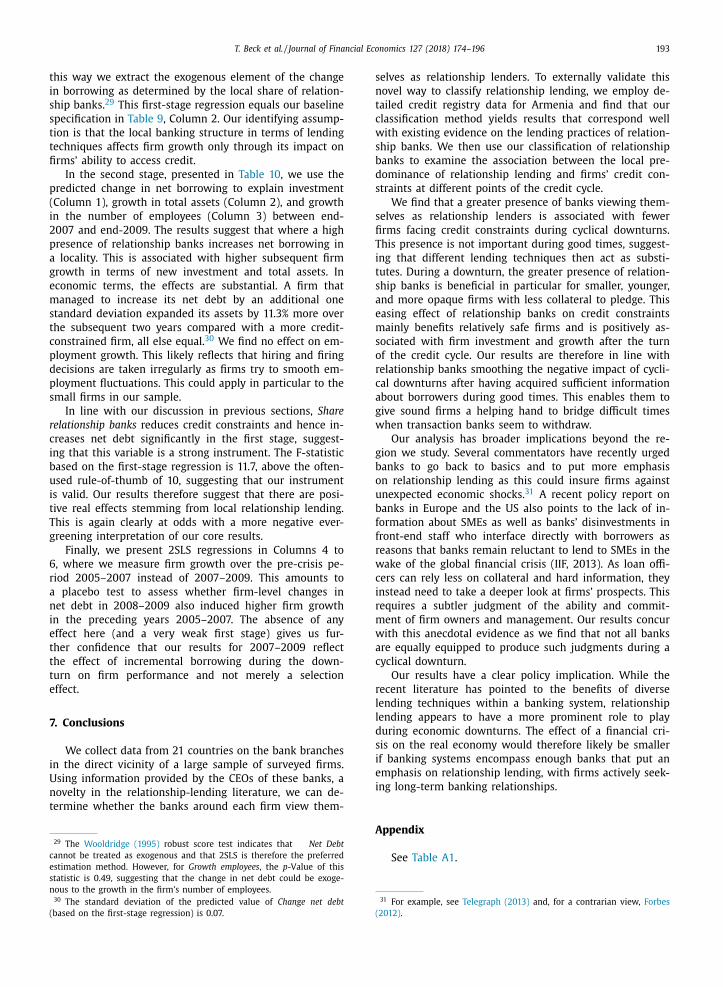
T. Beck et al. / Journal of Financial Economics 127 (2018) 174–196 193

this way we extract the exogenous element of the change

in borrowing as determined by the local share of relation-

ship banks. 29 This first-stage regression equals our baseline

specification in Table 9 , Column 2. Our identifying assump-

tion is that the local banking structure in terms of lending

techniques affects firm growth only through its impact on

firms’ ability to access credit.

In the second stage, presented in Table 10 , we use the

predicted change in net borrowing to explain investment

(Column 1), growth in total assets (Column 2), and growth

in the number of employees (Column 3) between end-

20 07 and end-20 09. The results suggest that where a high

presence of relationship banks increases net borrowing in

a locality. This is associated with higher subsequent firm

growth in terms of new investment and total assets. In

economic terms, the effects are substantial. A firm that

managed to increase its net debt by an additional one

standard deviation expanded its assets by 11.3% more over

the subsequent two years compared with a more credit-

constrained firm, all else equal. 30 We find no effect on em-

ployment growth. This likely reflects that hiring and firing

decisions are taken irregularly as firms try to smooth em-

ployment fluctuations. This could apply in particular to the

small firms in our sample.

In line with our discussion in previous sections, Share

relationship banks reduces credit constraints and hence in-

creases net debt significantly in the first stage, suggest-

ing that this variable is a strong instrument. The F-statistic

based on the first-stage regression is 11.7, above the often-

used rule-of-thumb of 10, suggesting that our instrument

is valid. Our results therefore suggest that there are posi-

tive real effects stemming from local relationship lending.

This is again clearly at odds with a more negative ever-

greening interpretation of our core results.

Finally, we present 2SLS regressions in Columns 4 to

6, where we measure firm growth over the pre-crisis pe-

riod 20 05–20 07 instead of 20 07–20 09. This amounts to

a placebo test to assess whether firm-level changes in

net debt in 20 08–20 09 also induced higher firm growth

in the preceding years 20 05–20 07. The absence of any

effect here (and a very weak first stage) gives us fur-

ther confidence that our results for 20 07–20 09 reflect

the effect of incremental borrowing during the down-

turn on firm performance and not merely a selection

effect.

7. Conclusions

We collect data from 21 countries on the bank branches

in the direct vicinity of a large sample of surveyed firms.

Using information provided by the CEOs of these banks, a

novelty in the relationship-lending literature, we can de-

termine whether the banks around each firm view them-

29 The Wooldridge (1995) robust score test indicates that � Net Debt

cannot be treated as exogenous and that 2SLS is therefore the preferred

estimation method. However, for Growth employees , the p -Value of this

statistic is 0.49, suggesting that the change in net debt could be exoge-

nous to the growth in the firm’s number of employees. 30 The standard deviation of the predicted value of Change net debt

(based on the first-stage regression) is 0.07.

selves as relationship lenders. To externally validate this

novel way to classify relationship lending, we employ de-

tailed credit registry data for Armenia and find that our

classification method yields results that correspond well

with existing evidence on the lending practices of relation-

ship banks. We then use our classification of relationship

banks to examine the association between the local pre-

dominance of relationship lending and firms’ credit con-

straints at different points of the credit cycle.

We find that a greater presence of banks viewing them-

selves as relationship lenders is associated with fewer

firms facing credit constraints during cyclical downturns.

This presence is not important during good times, suggest-

ing that different lending techniques then act as substi-

tutes. During a downturn, the greater presence of relation-

ship banks is beneficial in particular for smaller, younger,

and more opaque firms with less collateral to pledge. This

easing effect of relationship banks on credit constraints

mainly benefits relatively safe firms and is positively as-

sociated with firm investment and growth after the turn

of the credit cycle. Our results are therefore in line with

relationship banks smoothing the negative impact of cycli-

cal downturns after having acquired sufficient information

about borrowers during good times. This enables them to

give sound firms a helping hand to bridge difficult times

when transaction banks seem to withdraw.

Our analysis has broader implications beyond the re-

gion we study. Several commentators have recently urged

banks to go back to basics and to put more emphasis

on relationship lending as this could insure firms against

unexpected economic shocks. 31 A recent policy report on

banks in Europe and the US also points to the lack of in-

formation about SMEs as well as banks’ disinvestments in

front-end staff who interface directly with borrowers as

reasons that banks remain reluctant to lend to SMEs in the

wake of the global financial crisis (IIF, 2013). As loan offi-

cers can rely less on collateral and hard information, they

instead need to take a deeper look at firms’ prospects. This

requires a subtler judgment of the ability and commit-

ment of firm owners and management. Our results concur

with this anecdotal evidence as we find that not all banks

are equally equipped to produce such judgments during a

cyclical downturn.

Our results have a clear policy implication. While the

recent literature has pointed to the benefits of diverse

lending techniques within a banking system, relationship

lending appears to have a more prominent role to play

during economic downturns. The effect of a financial cri-

sis on the real economy would therefore likely be smaller

if banking systems encompass enough banks that put an

emphasis on relationship lending, with firms actively seek-

ing long-term banking relationships.

Appendix

See Table A1 .

31 For example, see Telegraph (2013) and, for a contrarian view, Forbes

(2012) .

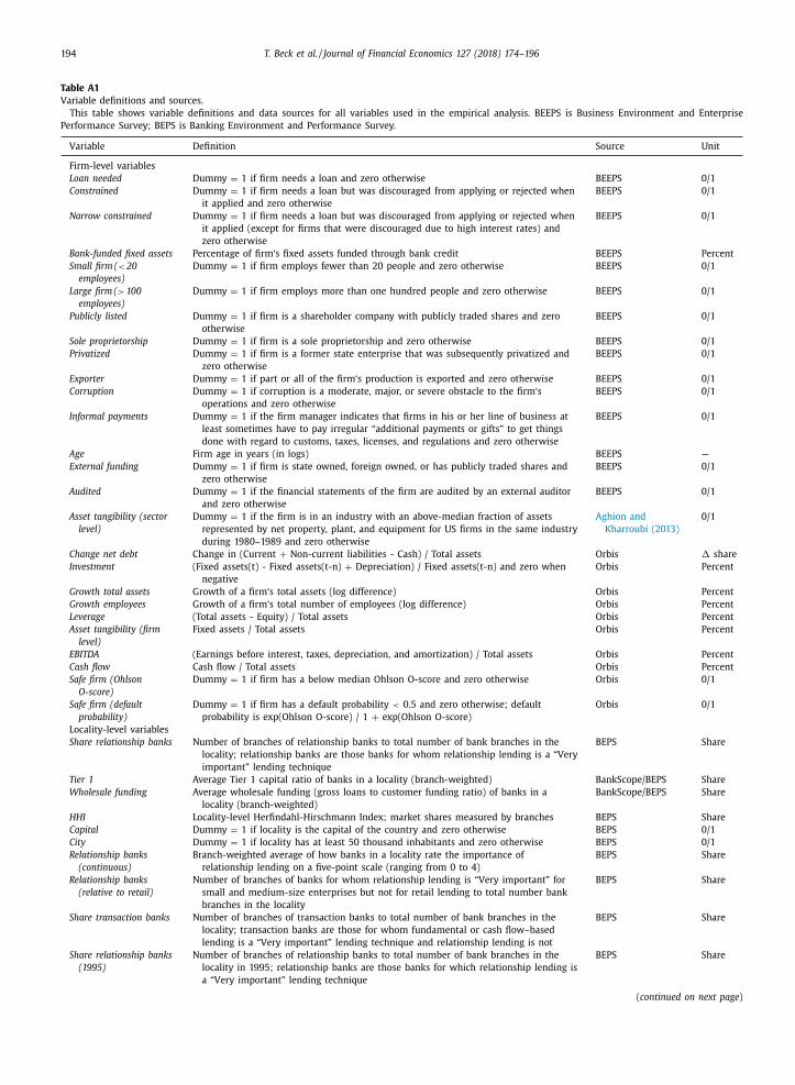
194 T. Beck et al. / Journal of Financial Economics 127 (2018) 174–196

Table A1

Variable definitions and sources.

This table shows variable definitions and data sources for all variables used in the empirical analysis. BEEPS is Business Environment and Enterprise

Performance Survey; BEPS is Banking Environment and Performance Survey.

Variable Definition Source Unit

Firm-level variables

Loan needed Dummy = 1 if firm needs a loan and zero otherwise BEEPS 0/1

Constrained Dummy = 1 if firm needs a loan but was discouraged from applying or rejected when

it applied and zero otherwise

BEEPS 0/1

Narrow constrained Dummy = 1 if firm needs a loan but was discouraged from applying or rejected when

it applied (except for firms that were discouraged due to high interest rates) and

zero otherwise

BEEPS 0/1

Bank-funded fixed assets Percentage of firm‘s fixed assets funded through bank credit BEEPS Percent

Small firm ( < 20

employees)

Dummy = 1 if firm employs fewer than 20 people and zero otherwise BEEPS 0/1

Large firm ( > 100

employees)

Dummy = 1 if firm employs more than one hundred people and zero otherwise BEEPS 0/1

Publicly listed Dummy = 1 if firm is a shareholder company with publicly traded shares and zero

otherwise

BEEPS 0/1

Sole proprietorship Dummy = 1 if firm is a sole proprietorship and zero otherwise BEEPS 0/1

Privatized Dummy = 1 if firm is a former state enterprise that was subsequently privatized and

zero otherwise

BEEPS 0/1

Exporter Dummy = 1 if part or all of the firm‘s production is exported and zero otherwise BEEPS 0/1

Corruption Dummy = 1 if corruption is a moderate, major, or severe obstacle to the firm‘s

operations and zero otherwise

BEEPS 0/1

Informal payments Dummy = 1 if the firm manager indicates that firms in his or her line of business at

least sometimes have to pay irregular “additional payments or gifts” to get things

done with regard to customs, taxes, licenses, and regulations and zero otherwise

BEEPS 0/1

Age Firm age in years (in logs) BEEPS —

External funding Dummy = 1 if firm is state owned, foreign owned, or has publicly traded shares and

zero otherwise

BEEPS 0/1

Audited Dummy = 1 if the financial statements of the firm are audited by an external auditor

and zero otherwise

BEEPS 0/1

Asset tangibility (sector

level)

Dummy = 1 if the firm is in an industry with an above-median fraction of assets

represented by net property, plant, and equipment for US firms in the same industry

during 1980–1989 and zero otherwise

Aghion and

Kharroubi (2013)

0/1

Change net debt Change in (Current + Non-current liabilities - Cash) / Total assets Orbis � share

Investment (Fixed assets(t) - Fixed assets(t-n) + Depreciation) / Fixed assets(t-n) and zero when

negative

Orbis Percent

Growth total assets Growth of a firm‘s total assets (log difference) Orbis Percent

Growth employees Growth of a firm‘s total number of employees (log difference) Orbis Percent

Leverage (Total assets - Equity) / Total assets Orbis Percent

Asset tangibility (firm

level)

Fixed assets / Total assets Orbis Percent

EBITDA (Earnings before interest, taxes, depreciation, and amortization) / Total assets Orbis Percent

Cash flow Cash flow / Total assets Orbis Percent

Safe firm (Ohlson

O-score)

Dummy = 1 if firm has a below median Ohlson O-score and zero otherwise Orbis 0/1

Safe firm (default

probability)

Dummy = 1 if firm has a default probability < 0.5 and zero otherwise; default

probability is exp(Ohlson O-score) / 1 + exp(Ohlson O-score)

Orbis 0/1

Locality-level variables

Share relationship banks Number of branches of relationship banks to total number of bank branches in the

locality; relationship banks are those banks for whom relationship lending is a “Very

important” lending technique

BEPS Share

Tier 1 Average Tier 1 capital ratio of banks in a locality (branch-weighted) BankScope/BEPS Share

Wholesale funding Average wholesale funding (gross loans to customer funding ratio) of banks in a

locality (branch-weighted)

BankScope/BEPS Share

HHI Locality-level Herfindahl-Hirschmann Index; market shares measured by branches BEPS Share

Capital Dummy = 1 if locality is the capital of the country and zero otherwise BEPS 0/1

City Dummy = 1 if locality has at least 50 thousand inhabitants and zero otherwise BEPS 0/1

Relationship banks

(continuous)

Branch-weighted average of how banks in a locality rate the importance of

relationship lending on a five-point scale (ranging from 0 to 4)

BEPS Share

Relationship banks

(relative to retail)

Number of branches of banks for whom relationship lending is “Very important” for

small and medium-size enterprises but not for retail lending to total number bank

branches in the locality

BEPS Share

Share transaction banks Number of branches of transaction banks to total number of bank branches in the

locality; transaction banks are those for whom fundamental or cash flow–based

lending is a “Very important” lending technique and relationship lending is not

BEPS Share

Share relationship banks

(1995)

Number of branches of relationship banks to total number of bank branches in the

locality in 1995; relationship banks are those banks for which relationship lending is

a “Very important” lending technique

BEPS Share

( continued on next page )

T. Beck et al. / Journal of Financial Economics 127 (2018) 174–196 195

Table A1 ( continued )

Variable Definition Source Unit

Share relationship banks

(20 0 0)

Number of branches of relationship banks to total number of bank branches in the

locality in 20 0 0; relationship banks are those banks for which relationship lending is

a “Very important” lending technique

BEPS Share

Lerner index Locality-level Lerner index; branch-weighted average of Lerner index as estimated for

each bank

BankScope/BEPS Share

Share foreign banks Number of branches of foreign-owned banks to total number of bank branches in the

locality

BEPS Share

Share small banks Number of branches of banks with less than 1 billion euros in assets to total number

of bank branches in the locality

BankScope/BEPS Share

Regional GDP growth Real gross domestic product growth in a region National sources Percent

References

Acharya, V.V. , Eisert, T. , Eufinger, C. , Hirsch, C. , 2014. Real Effects of theSovereign Debt Crisis in Europe: Evidence from Syndicated Loans.

Centre for Economic Policy Research, London, UK Discussion paper no.10108 .

Agarwal, S. , Hauswald, R. , 2010. Distance and private information in lend-

ing. Review of Financial Studies 23, 2757–2788 . Aghion, P. , Kharroubi, E. , 2013. Cyclical Macroeconomic Policy, Financial

Regulation, and Economic Growth. Bank for International Settlements,Basel, Switzerland Working paper no. 434 .

Ahlin, C. , Pang, T. , 2008. Are financial development and corruption controlsubstitutes in promoting growth? Journal of Development Economics

86 (2), 414–433 .

Ai, C. , Norton, E.C. , 2003. Interaction terms in logit and probit models.Economics Letters 80, 123–139 .

Altman, E. , 1968. Financial ratios, discriminant analysis and the predictionof corporate bankruptcy. Journal of Finance 23 (43), 589–609 .

Altonji, J.G. , Elder, T.E. , Taber, C.R. , 2005. Selection on observed and unob-served variables: assessing the effectiveness of Catholic schools. Jour-

nal of Political Economy 113 (1), 151–184 . Banerjee, R. , Gambacorta, L. , Sette, E. , 2016. The Real Effects of Relation-

ship Lending. Bank for International Settlements, Basel, Switserland

Unpublished working paper . Barnea, A. , Haugen, R.A. , Senbet, L.W. , 1980. A rationale for debt matu-

rity structure and call provisions in the agency theoretic framework.Journal of Finance 35, 1223–1234 .

Beck, T.H.L. , Demirgüc-Kunt, A. , Maksimovic, V. , 2005. Financial and legalconstraints to firm growth: does firm size matter? Journal of Finance

60, 137–177 .

Beck, T.H.L. , Ioannidou, V. , Schäfer, L. , 2017. Foreigners vs. natives: banklending technologies and loan pricing. Management Science forth-

coming . Bellows, J. , Miguel, E. , 2009. War and local collective action in Sierra

Leone. Journal of Public Economics 93 (11–12), 1144–1157 . Berger, A.N. , Miller, N.H. , Petersen, M.A. , Rajan, R.G. , Stein, J.C. , 2005. Does

function follow organizational form? Evidence from the lending prac-

tices of large and small banks. Journal of Financial Economics 76 (2),237–269 .

Berger, A.N. , Udell, G.F. , 1992. Some evidence on the empirical significanceof credit rationing. Journal of Political Economy 100 (5), 1047–1077 .

Berger, A.N. , Udell, G.F. , 1995. Relationship lending and lines of credit insmall business finance. Journal of Business 68, 351–381 .

Berlin, M. , Mester, L. , 1999. Deposits and relationship lending. Review of

Financial Studies 12 (3), 579–607 . Bharath, S.T. , Sandeep, D. , Saunders, A. , Srinivasan, A. , 2011. Lending rela-

tionships and loan contract terms. Review of Financial Studies 24 (4),1141–1203 .

Bliss, C. , Di Tella, R. , 1997. Does competition kill corruption? Journal ofPolitical Economy 105 (5), 1001–1023 .

Bolton, P. , Freixas, X. , Gambacorta, L. , Mistrulli, P.E. , 2016. Relationship and

transaction lending in a crisis. Review of Financial Studies 29 (10),2643–2676 .

Boot, A .W.A . , 20 0 0. Relationship banking: what do we know? Journal ofFinancial Intermediation 9, 7–25 .

Boot, A .W.A . , Thakor, A .V. , 1994. Moral hazard and secured lending in aninfinitely repeated credit market game. International Economic Re-

view 35, 899–920 .

Caballero, R.J. , Hoshi, T. , Kashyap, A.K. , 2008. Zombie lending and de-pressed restructuring in Japan. American Economic Review 98 (5),

1943–1977 .

Cameron, C.A. , Gelbach, J.B. , Miller, D.L. , 2008. Bootstrap-based improve-ments for inference with clustered errors. Review of Economics and

Statistics 90 (3), 414–427 .

Campello, M. , Graham, J.R. , Harvey, C.R. , 2010. The real effects of finan-cial constraints: evidence from a financial crisis. Journal of Financial

Economics 97 (3), 470–487 . Canales, R. , Nanda, R. , 2012. A darker side to decentralized banks: mar-

ket power and credit rationing in SME lending. Journal of FinancialEconomics 105, 353–366 .

Chemmanur, T.J. , Fulghieri, P. , 1994. Reputation, renegotiation, and thechoice between bank loans and publicly traded debt. Review of Fi-

nancial Studies 7, 475–506 .

Chodorow-Reich, G. , 2014. The employment effects of credit market dis-ruptions: firm-level evidence from the 20 08–20 09 financial crisis.

Quarterly Journal of Economics 129 (1), 1–59 . Claessens, S. , van Horen, N. , 2014. Foreign banks: trends and impact. Jour-

nal of Money, Credit, and Banking 46, 295–326 . Clarke, G.R. , Xu, L.C. , 2004. Privatization, competition and corruption: how

characteristics of bribe takers and payers affect bribes to utilities.

Journal of Public Economics 88 (9–10), 2067–2097 . Cox, D. , Japelli, T. , 1993. The effect of borrowing constraints on consumer

liabilities. Journal of Money, Credit, and Banking 25, 197–213 . Degryse, H. , Kim, M. , Ongena, S. , 2009. Microeconometrics of Banking:

Methods, Applications, and Results. Oxford University Press, Oxford,UK .

Degryse, H. , Ongena, S. , 2005. Distance, lending relationships, and compe-

tition. Journal of Finance 60, 231–266 . Degryse, H. , Van Cayseele, P. , 20 0 0. Relationship lending within a

bank-based system: evidence from European small business data.Journal of Financial Intermediation 9 (1), 90–109 .

De Haas, R.T.A. , Korniyenko, Y. , Pivovarsky, A. , Tsankova, T. , 2015. Tamingthe herd? Foreign banks, the Vienna Initiative and crisis transmission.

Journal of Financial Intermediation 24 (3), 325–355 .

DeYoung, R. , Gron, A. , Torna, G. , Winton, A. , 2015. Risk overhang and loanportfolio decisions: small business loan supply before and during the

financial crisis. Journal of Finance 70 (6), 2451–2488 . Djankov, S. , La Porta, R. , Lopez-De-Silanes, F. , Shleifer, A. , 2002. The regu-

lation of entry. Quarterly Journal of Economics 117 (1), 1–37 . Duca, J. , Rosenthal, S. , 1993. Borrowing constraints, household debt, and

racial discrimination in loan markets. Journal of Financial Intermedia-

tion 3, 77–103 . Duchin, R. , Ozbas, O. , Sensoy, B.A. , 2010. Costly external finance, corpo-

rate investment, and the subprime mortgage credit crisis. Journal ofFinancial Economics 97, 418–435 .

Fahlenbrach, R. , Prilmeier, R. , Stulz, R.M. , 2012. This time is the same: us-ing bank performance in 1998 to explain bank performance during

the recent financial crisis. Journal of Finance 67, 2139–2185 .

Forbes, 2012. Let’s abolish Wall Street and return to local banking!September 13.

Gale, D. , Hellwig, M. , 1985. Incentive-compatible debt contracts: theone-period problem. Review of Economic Studies 52, 647–663 .

Gennaioli, N. , La Porta, R. , Lopez de Silanes, F. , Shleifer, A. , 2014. Growthin regions. Journal of Economic Growth 19, 259–309 .

Gobbi, G. , Sette, E. , 2014. Do firms benefit from concentrating their bor-rowing? Evidence from the Great Recession. Review of Finance 18 (2),

527–560 .

Heckman, J.J. , 1979. Sample selection bias as a specification error. Econo-metrica 47 (1), 153–161 .

Hosmer, D.W. , Lemeshow, S. , 2013. Applied Logistic Regression. Wiley In-stitute of International Finance, New York .

196 T. Beck et al. / Journal of Financial Economics 127 (2018) 174–196

Iyer, R. , Peydró, J.-L. , da-Rocha-Lopes, S. , Schoar, A. , 2014. Interbank liquid- ity crunch and the firm credit crunch: evidence from the 20 07–20 09

crisis. Review of Financial Studies 27 (1), 347–372 . Jiménez, G. , Ongena, S. , Peydró, J.-L. , Saurina, J. , 2012. Credit supply and

monetary policy: identifying the bank balance-sheet channel with loan applications. American Economic Review 102, 2301–2326 .

Johnson, S. , Kaufmann, D. , McMillan, J. , Woodruff, C. , 20 0 0. Why do firms

hide? Bribes and unofficial activity after communism. Journal of Pub- lic Economics 76, 495–520 .

Kysucky, V. , Norden, L. , 2016. The benefits of relationship lending in a cross-country context: a meta-analysis. Management Science 62,

90–110 . McIntosh, C. , Dorfman, J. , 1992. Qualitative forecast evaluation: a compar-

ison of two performance measures. American Journal of Agricultural Economics 74 (1), 209–214 .

Mian, A.R. , 2006. Distance constraints: the limits of foreign lending in

poor economies. Journal of Finance 61, 1465–1505 . OECD, 2015. Financing SMEs and Entrepreneurs: An OECD Scoreboard. Or-

ganization for Economic Co-operation and Development, Paris, France . Ohlson, J.A. , 1980. Financial ratios and the probabilistic prediction of

bankruptcy. Journal of Accounting Research 18 (1), 109–131 . Ongena, S. , Popov, A. , Udell, G.F. , 2013. When the cat’s away the mice will

play: does regulation at home affect bank risk-taking abroad? Journal

of Financial Economics 108 (3), 727–750 . Ongena, S. , Smith, D.C. , 2001. The duration of bank relationships. Journal

of Financial Economics 61 (3), 449–475 . Peek, J. , Rosengren, E.S. , 2005. Unnatural selection: perverse incentives

and the misallocation of credit in Japan. American Economic Review

95 (4), 1144–1166 .

Petersen, M. , 1999. Banks and the role of lending relationships: evidence

from the US experience. Northwestern University, Evanston, Il, Unpub- lished working paper .

Petersen, M. , Rajan, R.G. , 1994. The benefits of lending relationships: evi- dence from small business data. Journal of Finance 49, 1367–1400 .

Petersen, M. , Rajan, R.G. , 2002. Does distance still matter? The informa- tion revolution in small business lending. Journal of Finance 57 (6),

2533–2570 . Popov, A. , Udell, G.F. , 2012. Cross-border banking, credit access, and the

financial crisis. Journal of International Economics 87, 147–161 . Puri, M. , Rocholl, J. , Steffen, S. , 2011. Global retail lending in the aftermath

of the US financial crisis: distinguishing between supply and demand

effects. Journal of Financial Economics 100, 556–578 . Rajan, R.G. , 1992. Insiders and outsiders: the choice between relationship

and arm’s length debt. Journal of Finance 47, 1367–1400 . Santikian, L. , 2014. The ties that bind: bank relationships and small busi-

ness lending. Journal of Financial Intermediation 23 (2), 177–213 . Sch ӓfer, L. , 2016. Forgive but not forget: the behavior of relationship banks

when firms are in distress. Frankfurt School of Finance & Manage- ment, Frankfurt, Germany Unpublished working paper .

Sette, E. , Gobbi, G. , 2015. Relationship lending during a financial crisis.

Journal of the European Economic Association 13 (3), 453–481 . Svensson, J. , 2003. Who must pay bribes and how much? Evidence from

a cross section of firms. Quarterly Journal of Economics 118 (1), 207–230 .

Telegraph, 2013. Local banks for local people. May 28. Thakor, A.V. , Udell, G.F. , 1991. Secured lending and default risk: equi-

librium analysis, policy implications and empirical results. Economic

Journal 101, 458–472 . Uchida, H. , Udell, G.F. , Yamori, N. , 2012. Loan officers and relationship

lending to SMEs. Journal of Financial Intermediation 21, 97–122 . Von Thadden, E.L. , 1995. Long-term contracts, short-term investment, and

monitoring. Review of Economic Studies 62 (4), 557–575 . Wooldridge, J.M. , 1995. Score diagnostics for linear models estimated by

two-stage least squares. In: Maddala, G., Phillips, P., Srinivasan, T.

(Eds.), Advances in Econometrics and Quantitative Economics. Black- well, Oxford, UK, pp. 66–87 .