Journal of Experimental Marine Biology and Ecology 471 (2015) 64–76

Contents lists available at ScienceDirect

Journal of Experimental Marine Biology and Ecology

j ourna l homepage: www.e lsev ie r .com/ locate / jembe

Ecology of the Ocean Sunfish, Mola mola, in the southern CaliforniaCurrent System

Tierney M. Thys a,⁎, John P. Ryan b, Heidi Dewar c, Christopher R. Perle d, Kady Lyons e, John O'Sullivan f,Charles Farwell f, Michael J. Howard f, Kevin C. Weng g, Bertha E. Lavaniegos h, Gilberto Gaxiola-Castro h,Luis Erasmo Miranda Bojorquez h, Elliott L. Hazen i, Steven J. Bograd i

a California Academy of Sciences, San Francisco, CA 94118, USAb Monterey Bay Aquarium Research Institute, Moss Landing, CA 95039, USAc NOAA Fisheries, SWFSC, La Jolla, CA 92037, USAd Florida State College, Jacksonville, FL 32256, USAe University of Calgary, Calgary, AB T2N 1N4, Canadaf Monterey Bay Aquarium, Monterey, CA 93940, USAg Virginia Institute of Marine Science, Gloucester Point, VA 23062-1346, USAh Centro de Investigación Científica y Educación Superior de Ensenada, Departamento de Oceanografía Biológica, Ensenada, Baja California C.P. 22860, Mexicoi Environmental Research Division, Southwest Fisheries Science Center, NOAA Fisheries, Pacific Grove, CA, USA

⁎ Corresponding author. Tel.: +1 831 277 6763.E-mail addresses: tierneythys@gmail.com (T.M. Thys)

Heidi.Dewar@noaa.gov (H. Dewar), chperle@fscj.edu (C.Rkady.lyons@sbcglobal.net (K. Lyons), JOSullivan@mbayaqCFarwell@mbayaq.org (C. Farwell), mhoward@mbayaq.orkevinweng@vims.edu (K.C. Weng), berlav@cicese.mx (B.Eggaxiola@cicese.mx (G. Gaxiola-Castro), lmiranda@ciceseBojorquez), Elliott.Hazen@noaa.gov (E.L. Hazen), Steven.B

http://dx.doi.org/10.1016/j.jembe.2015.05.0050022-0981/© 2015 The Authors. Published by Elsevier B.V

a b s t r a c t

a r t i c l e i n f o

Article history:Received 25 March 2015Received in revised form 4 May 2015Accepted 5 May 2015Available online xxxx

Keywords:California CurrentFrontsGelatinous zooplanktonOcean sunfishRemote sensingSatellite tagging

The common ocean sunfish,Molamola, occupies a unique position in the eastern Pacific Ocean and the CaliforniaCurrent Large Marine Ecosystem (CCLME) as the world's heaviest, most fecund bony fish, and one of the mostabundant gelativores.M. mola frequently occur as bycatch in fisheries worldwide and comprise the greatest por-tion of the bycatch in California's large-mesh drift gillnetfishery. In this first long-term tagging study of any oceansunfish species in the eastern Pacific, 15M.mola (99 cm to 200 cm total length) were tagged in the southern Cal-ifornia Bight (SCB) between 2003 and 2010 using 14 satellite pop-off archival tags (PATs) and one Fastloc Mk10GPS tag. Ten tags provided positional data for a cumulative dataset of 349 tracking days during themonths of JulythroughMarch. Thirteen tags provided temperature and depth data. AllM.mola remainedwithin ~300 kmof thecoast, and nearly all exhibited seasonalmovement between the SCB and adjacent waters off northern and centralBaja California, Mexico. No tagged individuals were tracked north of the SCB. Tag depth data showed diel verticalmigration and occasional deep (N500 m) dives. Data from the Fastloc GPS tag allowed close examination of therelationship between the movements of the largest tagged ocean sunfish (2 m TL) and fine-scale oceanographicfeatures. Near-instantaneous satellite sea surface temperature images showed this individual associatedwith up-welling fronts along itsmigration path, which exceeded 800 kmand ranged from6 to 128 km from the coast. Tagdepth data showed active use of the water column within the frontal zones. Synthetic aperture radar (SAR) im-ages demonstrated that surface slicks, which often indicate convergent circulation, coincided with this type offront. Zooplankton tows in the southern region of tracking off central Baja California,Mexico revealed dense pop-ulations of salps toward the warm side of these fronts. Satellite tag and ecosystem data suggest that bio-physicalinteractions in coastal upwelling fronts create favorable foraging habitat.

© 2015 The Authors. Published by Elsevier B.V. This is an open access article under the CC BY-NC-ND license(http://creativecommons.org/licenses/by-nc-nd/4.0/).

, ryjo@mbari.org (J.P. Ryan),. Perle),.org (J. O'Sullivan),g (M.J. Howard),. Lavaniegos),.edu.mx (L.E. Mirandaograd@noaa.gov (S.J. Bograd).

. This is an open access article under

1. Introduction

Satellite tracking has allowed new insights into the behavioralecology of a range of taxa including many marine megafauna suchas turtles, whales, seals, fish and squid (Block et al., 2011; Costaet al., 2012). Such studies are providing valuable information forfisheries and the management of ecosystems. One species that hasattracted attention, due in part to its diet and unique morphology,isMolamola (Linnaeus, 1758), the common ocean sunfish. Inhabitingall tropical and temperate ocean regions, this species obtains thegreatest adult mass of any teleost fish and has the greatest fecundity

the CC BY-NC-ND license (http://creativecommons.org/licenses/by-nc-nd/4.0/).

Fig. 1. Tagging studies of ocean sunfish. (A) Photograph of satellite-taggedMolamola off SanDiego, California USA. Fish TL=1.1m. (B)MODIS Aqua 2013 average sea surface temperature(SST), representing regions inwhich long-term tagging studies ofM.mola have occurred, including northwestern Pacific (1) and the northwestern, northeastern and southeastern Atlantic(2–4). The present study in the southern California Current Large Marine Ecosystem (CCLME, arrow) is the first long-term tagging study ofM. mola in the eastern Pacific.(A) Photo by Mike Johnson, 2006.

65T.M. Thys et al. / Journal of Experimental Marine Biology and Ecology 471 (2015) 64–76

(Carwardine, 1995; Roach, 2003; Schmidt, 1921). Beyond their phys-iological distinctions and unusual shape (Fig. 1A), ocean sunfish arealso distinguished by their role in the marine food web. Largeocean sunfish (N1 m total length [TL]) primarily consume gelatinouszooplankton and are the most abundant and largest gelativore in theworld ocean (Cardona et al., 2012; Harrod et al., 2013; Nakamura andSato, 2014).

Ocean sunfish comprise a large percentage of bycatch in gillnet andtrawl fisheries worldwide, e.g. 70–95% of total catch in the Mediterra-nean Sea drift gillnet fishery (DGN) which targets swordfish (genusXiphias) (Silvani et al., 1999; Tudela et al., 2005) and 29–76% of totalcatch in the South African mid-water trawl fishery, which targetshorse mackerel (family Carangidae) (Petersen, 2005; Petersen andMcDonell, 2007). In California's DGN fishery, which targets swordfish(Xiphias gladius), M. mola comprise 14–61% of the total catch (NationalOceanic and Atmospheric Administration (NOAA), unpublished data).Observers report that most individuals (N95%) are released alive(www.westcoast.fisheries.noaa.gov) although they also note that somefish (an estimated 40% D. Cartamil, pers comm, Feb 18, 2015) show obvi-ous signs of fishery-induced trauma, including loss of protective mucus,abrasions and bleeding (Cartamil and Lowe, 2004). Post-release survivalrate for M. mola is unknown in all drift gillnet fisheries. Studies ofM.mola ecology and behavior are thusmotivated by thewidespreaddis-tribution of the species in vastly different oceanic habitats, its trophicrole, reproductive potential and prevalence as bycatch.

M. mola is a seasonal inhabitant in the southern California CurrentLarge Marine Ecosystem (CCLME) (Bass et al., 2005; Cartamil andLowe, 2004). In contrast to the western Pacific where at least two sub-species have been suggested to occur, Mola sp. A and Mola sp. B(Sawai et al., 2011; Yoshita et al., 2009), no sub-species of the Molagenus have been reported in genetic studies of M. mola in the CCLME(Bass et al., 2005). Ocean sunfish have long been residents in this region.Molid fossils from the Miocene have been found along the Californiacoast (Hakel and Stewart, 2002) and archeological sites dating back to8500 yrs bp suggest a robust prehistoric ocean sunfish fishery onceexisted along the central and southern California coast (Joslin, 2012;Porcasi and Andrews, 2001). Currently, there are no commercial fisheryoperations targetingM. mola in this region.

The southern CCLME is a comprehensively studied oceanographicregionwith numerous long-termenvironmental datasets that are usefulfor understanding fish movements and behaviors. The longest runningextant datasets include the California Cooperative Oceanic Fisheries In-vestigations (CalCOFI) records of hydrographic and plankton samplingoff the California coast and the Investigaciones Mexicanas de laCorriente de California (IMECOCAL) operations off Baja California,Mexico. Recently the CCLME has been forecast to be impacted signifi-cantly by ocean acidification (Hofmann et al., 2014) and changing

ocean temperatures (NOAA, 2014). This region thus provides an ideallocation to investigate the relationships between M. mola ecology,oceanographic processes and fishery interactions within the context ofbroader human impacts.

Previous studies of M. mola have yielded valuable insights with re-gard to natural history, movements and behaviors (Pope et al., 2010).Cartamil and Lowe (2004) investigated short-term (up to 3 days)move-ments ofM. mola in the SCB using acoustic tags and continuous manualtracking. This study found that individuals moved a mean distance of26.8 ± 5.2 km d−1 and repeatedly dove below the thermocline duringthe day. Individuals remained above the thermocline at night and ex-hibited less overall vertical movement. Long-term (N3 months) pop-up satellite tagging studies of M. mola in the northwestern Pacific(Dewar et al., 2010) and 3 regions of the Atlantic (Sims et al., 2009a,b;Potter and Howell, 2011; Fig. 1B) show no evidence of M. mola move-ments across ocean basins, but rather protracted occupation withinhemispheric oceanmargins. In these studies, latitudinal movement pat-terns correlatedwith seasonal changes in temperature andproductivity,which likely indicate favorable thermal and foraging habitats (Dewaret al., 2010; Potter et al., 2011; Sims et al., 2009a).

This study examines regional and seasonal movement patterns ofM. mola tagged between 2003 and 2010. Fastloc GPS data from onetag were integrated with concurrent observations from satellite remotesensing to examinehabitat use. These datawere coupledwithfine-scaleship sampling to explore forage species distributions in relation to hab-itat. The goal of this study was to provide a greater understanding ofM. mola ecology, its relationships with oceanographic features and itsseasonal movement patterns to help inform fisheries and ecosystemmanagement.

2. Materials and methods

2.1. Tagging and species identification

M. molawere tagged in the SCB from July through October between2003 and 2010 (Table 1). Fish were tagged either opportunistically dur-ing a research longline cruise (n= 4) or during dedicated tagging tripson a small vessel (n = 11). During the dedicated tagging trips, M. molawere located from a boat or from a spotter plane (pilot: D. Mauer,Carlsbad, CA, USA) that relayed fish locations via a hand-held radio tocrew on a 7 m boat. Free-swimming fish were captured using a 1 mdiameter salmon net, and only healthy individuals without obviouswounds or visibly heavy parasite loads were selected for tagging.Individualswere then brought next to the boat,measured to the nearestcm and tagged in thewater. A small incisionwasmade below the dorsalfin and a nylon dart, attached to the tags with 300-pound testmonofilament line and stainless steel crimps (Fig. 1A), was inserted

Table 1Tag deployment summary.

PTTTag type

Tag ID DeployPop-off

Size (cm)Weight (kg)

DeployLat (°N)Lon (°W)

Pop offLat (°N)Lon (°W)

DeploymentDurationTracking days

Distance (km)

41742PAT

03P0266a Sep 6 03Sep 25 03

11682

32.88117.3

33.55118.14

17b –

41749PAT

03P0245a Sep 6 03Sep 25 03

11784

32.97117.5

32.86118.11

14b

849.5

41752PAT

03P0248 Sep 6 03Mar 21 04

143152

32.89117.3

32.89117.91

19871

55.0

41756PAT

03P0216 Sep 6 03Mar 21 04

150175

32.99117.5

26.50114.39

196b –

41767PAT

02P0201 Sep 6 03Mar 22 04

11784

32.91117.4

27.15116.19

19858

600.9

61919PAT

05P0157 Oct 5 06Mar 28 07

131117

32.92117.5

31.01117.59

17434

212.7

61920PAT

05P0158 Oct 1 06Mar 31 07

133123

32.85117.4

31.17116.82

181b 195.1

61922PAT

05P0160 Oct 1 06Mar 30 07

130115

32.86117.4

29.30115.22

18038

445.0

61924PAT

05P0171 Oct 1 06Mar 29 07

131117

32.84117.4

30.61116.91

17940

256.9

63978PAT

05P0245 Jul 6 06c

Mar 04 0792d 32.83

117.828.62115.21

241b 530.1

63980PAT

05P0247 Jul 12 06c

Mar 09 07150175

33.12118.3

32.77120.28

24010

182.8

63983PAT

05P0250 Jul 12 06c

Mar 09 07132120

33.12118.3

31.62117.54

24023

185.5

77160PAT

07A0158 Jul 27 07Jan 23 08

9951

33.19119.2

30.68116.47

18118

392.9

91973MiniPAT

09P0101 Aug 21 09c

Nov 19 09127107

33.40118.2

28.25115.06

90b –

89297Fastloc

10A0564 Aug 28 10Dec 25 10

200412

32.88117.5

25.90112.84

11949

893.9

– insufficient data for track analysis.Size is total length. Weight is estimated from previously published length/weight relationships (Watanabe and Sato, 2008).

a Premature release and presumed mortality.b Insufficient data for tracking or omitted from Fig. 2 for clarity due to shortness of track.c Tags deployed during longline trips.d Pre-caudal length.

66 T.M. Thys et al. / Journal of Experimental Marine Biology and Ecology 471 (2015) 64–76

with a tag applicator. A pectoral fin clip was taken for genetic analysisbefore tagged fish were released: all species were later confirmed asM. mola using mitochondrial DNA analyses (S. Karl and J. Whitney, un-published data). The entire process was completed in approximately2–5 min. To ensure proper tag placement and active movements post-tagging, a snorkeler monitored fish visually for up to 5 min. All animalstagged in this manner exhibited strong, healthy swimming movementafter tagging with no visible interference from the tag.

During the research cruises, M. mola were caught on a longline andpulled into a cradle secured to the boat for tagging. The methods fortag insertion were the same as those used for free-swimming individ-uals. Following tagging, total length was recorded to the nearest centi-meter and a fin clip was taken. The hook was then removed and thefish was released.

Tags deployed included several versions of pop-up satellite tags(PSAT: PAT, mini-PAT, MK10 PAT, MK10-AF PAT [Fastloc GPS], WildlifeComputers, Redmond,WA, U.S.A.) (Fig. 1A; Table 1). The tags were pro-grammed to release after periods ranging from 1 to 9 months. PAT de-vices collected data on ambient temperature, depth and light intensity(measured as irradiance at 550 nm) every 1–2 min. Fastloc GPS tag col-lected and archived data every second. Archived PAT datawere summa-rized on-board, and summaries were transmitted after the tag releasedfrom the animal. The Fastloc GPS tag data were transmitted along thetrack and post release.

2.2. Tag horizontal data and analyses

The first 24 h of each trackwas removed because some degree of be-havior modification is expected after tagging (Hoolihan et al., 2011).

Tags providing fewer than 7 estimated geolocations were excludedfrom the horizontal analyses (Table 1). Transmitted data were decodedwith Wildlife Computers DAP(R) Processor (www.wildlifecomputers.com). The geolocation routines Trackit (Nielsen and Sibert, 2007) andTrackitSST (Lam et al., 2010), executed in R Statistical Software (RDevelopment Core Team, 2013) using default settings, were used to es-timate geolocation. Results from TrackitSSTwere preferred because thisroutine combines sea surface temperature (SST) data with a Kalman-filter state spacemovementmodel to producemore precise geolocationestimates (Lam et al., 2010; Nielsen et al., 2006). If TrackitSST failed toconverge on a resultant track (possibly as a result of unavailable SSTdata), Trackit was used. The geolocation results of estimated latitudesand longitudes and their associated uncertainties were then importedback into DAP Processor.

The Fastloc GPS electronic tag 89297 transmitted both GPS andArgos quality locations along its track whenever the tag was above thewater for a sufficient time interval to turn on. Once data were decoded(as per above), the DAP Processor Fast-GPS solver used Receiver Inde-pendent Exchange Format (RINEX) files to post-process transmitted po-sitions to improve accuracy. On days when GPS solutions were notavailable, Argos positions calculated from N4 uplinks were used toserve as possible along-track substitutes for missing GPS data (n = 2).

2.3. Vertical data

Mortalities were excluded from vertical analysis. Mortalities werepresumed when depth remained constant for 72 h or when depthexceeded 1500 m, both of which trigger release of the tag. Verticaldata were analyzed using transmitted time-at-depth (TAD) and time-

67T.M. Thys et al. / Journal of Experimental Marine Biology and Ecology 471 (2015) 64–76

at-temperature (TAT) histograms and profiles of depth and tempera-ture (PDT) data that consisted of 8 temperature and depth measure-ments over the depth range encountered in a given time interval(Table 2). Data were summarized over programmed time intervals setat 6, 12 and 24 h, depending on the tag. Diel patterns were examinedwhen possible. Tags with bins set at 12 h (n = 3) or 24 h (n = 1)could not exclusively provide day or night intervals, so their data wereexcluded from diel analysis. Tag 77160 was also excluded since it usedan alternate binning scheme. For the 9 tags set at 6 h intervals, the dayintervals spanned from 9 am to 3 pm and night from 9 pm to 3 am.

The maximum and minimum temperatures and depths werecalculated for each day and night separately and these daily valueswere averaged for each individual fish (Table 2). Temperature anddepth histograms contained 11 to 14 bins based on the binning schemeprogrammed into the tag. Over the course of the study, tags were de-ployedwith different binning schemes. Due to this inconsistency, histo-grams were calculated across schemes using methods described inDewar et al. (2011). For example, temperature bins spread across oddnumbers (13–15, 15–17) can be converted to even numbers (12–14,14–16) by dividing the values for each of the odd bins in half. This pro-vides an estimate for bins of 1 °C width. These bins were then summedaccordingly to create common bins. This process assumes that distribu-tion across bins is equal, which may not always be the case, and conse-quently normalizing in this manner may reduce precision. A separatetime series contour plot wasmade for Fastloc tag 89297 since it provid-ed the highest resolution combination of histogram and location data.

2.4. Satellite remote sensing data and analyses for Fastloc GPS tracking

The high temporal resolution and small error of Fastloc GPS positiondata (b0.1 km) compared to the fewer positions and larger error (tensto hundreds of kms depending on location class, www.argos-system.org), allowed examination of relationships between an individual fish(tag 89297) and fine-scale ocean features using satellite remote sensingdata. These analyses were constrained to the period of August 30through October 27, 2010, after which the tag provided only one loca-tion until its pop-off date of December 25, 2010.

Table 2Tag temperature and depth data.

PTT Bin Interval (h) SST (°C) range Min temp ± SD (°C)

Day Night

41752 12a 16(13.8–21.0)

10 ± 1.4(8–14)

11 ± 1.5(8–15)

41756 12a 19(15.8–23.4)

10 ± 1.5(8–15)

12 ± 2.6(9–19)

41767 12a 18(15.0–21.1)

11 ± 1.5(8–16)

12 ± 2.3(9–17)

61919 6 16(14–19)

10 ± 1.5(8–14)

15 ± 1.5(12–17)

61920 6 15(12–18)

10 ± 0.6(9–11)

13 ± 1.3(11–14)

61922 6 17(15–23)

11 ± 2.1(8–16)

15 ± 1.7(12–16)

61924 6 18(14–23)

10 ± 1.7(9–13)

14 ± 2.4(12–17)

63978 6 18(18–23)

12 ± 2.3(16–19)

14 ± 1.3(12–16)

63980 6 21(20–21)

11 ± 2.8(9–13)

12 ± 0.4(12–13)

63983 6 18(7–24)

10 ± 1.0(9–13)

13 ± 2.1(8–16)

77160 6a 19(14–20)

9 ± 0.9(8–11)

14 ± 2.1(11–20)

89297 6 19(16–22)

12 ± 3.2(0–18)

14 ± 2.4(7–19)

91973 24a 21(20–24)

– –

a Not included in Fig. 3 due to bin incompatibility.

2.4.1. Habitat occupation in relation to sea surface temperature (SST)Data for examining fish movements in relation to physical oceanog-

raphy were derived from archived CoastWatch SST (http://coastwatch.pfeg.noaa.gov/erddap/). To increase the potential for matchupsbetween GPS positions and SST images, data from both the AdvancedVery High Resolution Radiometer (AVHRR) and the Moderate Resolu-tion Imaging Spectroradiometer (MODIS) Aqua sensor were obtained.AVHRR data prior to application of cloud removal algorithms were ex-amined to ensure that valid SST data were not lost by inaccurate cloudremoval. When AVHRR and MODIS images were available for nearlythe same time, the image having better coverage of the region occupiedby theM. mola was selected.

2.4.2. Habitat characterization from synthetic aperture radar (SAR)SAR data describes ocean surface roughness and can identify

features such as slicks, internal waves and other physical phenomena(Apel, 2004; Holt, 2004; Lyzenga et al., 2004). Slicks identified by SARimages can indicate convergent frontal zones (Holt, 2004), and this ca-pability has been useful in coastal plankton ecology research (e.g. Ryanet al., 2005, 2008, 2010). Archived SAR images from the European SpaceAgencywere used to examine the nature of oceanic fronts in regions oc-cupied by the Fastloc tagged fish. The SAR image search was conductedusing the EOLI–SA interface (http://earth.esa.int/EOLi/EOLi.html). Theonly sensor that had acquired SAR images in the region and period ofthe fish tracking was ENVISAT ASAR. These images had a spatial resolu-tion of approximately 30m. Although no SAR images could provide cov-erage exactly when and where the fish was located, two SAR imageswerematchedwith SST images to examine fronts detected in the great-er study region during the tag deployment period.

2.5. Fine-scale habitat and forage species characterization

In situ oceanographic data were obtained from IMECOCAL cruiseIM1010 (October 2010) including data from a profiling CTD with a dis-solved oxygen sensor, an underway surface thermosalinograph, andbongo net macrozooplankton collections. Zooplankton displacementvolumewasmeasured from the complete sample and functional groups

Max depth (m) Min depth ± SD (m) Max depth ± SD (m)

Day Night Day Night

336 4 ± 34.1(0–0)

4 ± 13.8(0–88)

177 ± 82(16–300)

80 ± 60.5(0–292)

556 0 ± 4.0(0–0)

9 ± 20.2(0–84)

223 ± 80(0–404)

80 ± 60.5(0–292)

356 2 ± 8.8(0–0)

3 ± 14.9(0–56)

209 ± 75(16–308)

121 ± 87.7(0–248)

316 13 ± 60.1(0–8)

4 ± 7.0(0–8)

182 ± 117(0–316)

30 ± 18.6(0–88)

360 49 ± 116(0–0)

2 ± 2.2(0–4)

203 ± 76(88–268)

42 ± 37.9(0–100)

512 20 ± 51.5(0–0)

2 ± 4.0(0–8)

168 ± 94(0–284)

31 ± 21.0(0–76)

400 15 ± 36.1(0–96)

2 ± 3.1(0–8)

173 ± 119(0–292)

25 ± 14.2(4–48)

312 1 ± 3.6(0–0)

8 ± 20.7(0–68)

96 ± 89(0–296)

66 ± 26.9(24–104)

336 0 ± 0(0–0)

0 ± 0(0–0)

100 ± 141(0–200)

30 ± 8.5(24–36)

396 10 ± 37.1(0–0)

3 ± 6.7(0–0)

208 ± 810–320

36 ± 32.90–144

504 1 ± 6.1(0–0)

1 ± 2.2(0–8)

209 ± 61(72–273)

36 ± 16.2(16–64)

520 23 ± 22.2(0–88)

9 ± 9.2(0–40)

139 ± 84.6(0–520)

73 ± 73(16–520)

312 – – – –

68 T.M. Thys et al. / Journal of Experimental Marine Biology and Ecology 471 (2015) 64–76

were counted from a fraction (1/8) of selected samples. Collectionmethodologies are described in Lavaniegos et al. (2002) with the oneexception being that macrozooplankton for cruise IM1010were collect-ed with a 71 cm instead of a 61 cm diameter bongo net.

3. Results and discussion

3.1. Tag and geolocation performance

Thirteen out of the 15 tags remained attached for their set deploy-ments with durations ranging from 90 to 241 days (Table 1). The twotags that released prematurely, 41742 (17 days) and 41749 (14 days),indicated fish mortality. Tag 41742 was retrieved and its data revealedit remained at 76–80 m for 3 days before releasing. Tag 41749 sank toa depth N980 m, released and initiated transmission at the surfaceafter 3 days. The fact that both these animals diedwithin similar periodsfollowing release suggests that tagging may have been a possible causeof death.With additional tagging and a large enough sample size, it maybe feasible to estimatemortalitywithin this population as has been sug-gested by previous studies on marine turtles (Hays et al., 2003). Tags41756, 61920, 63978 and 91973 did not provide sufficient geolocationdata for track analysis.

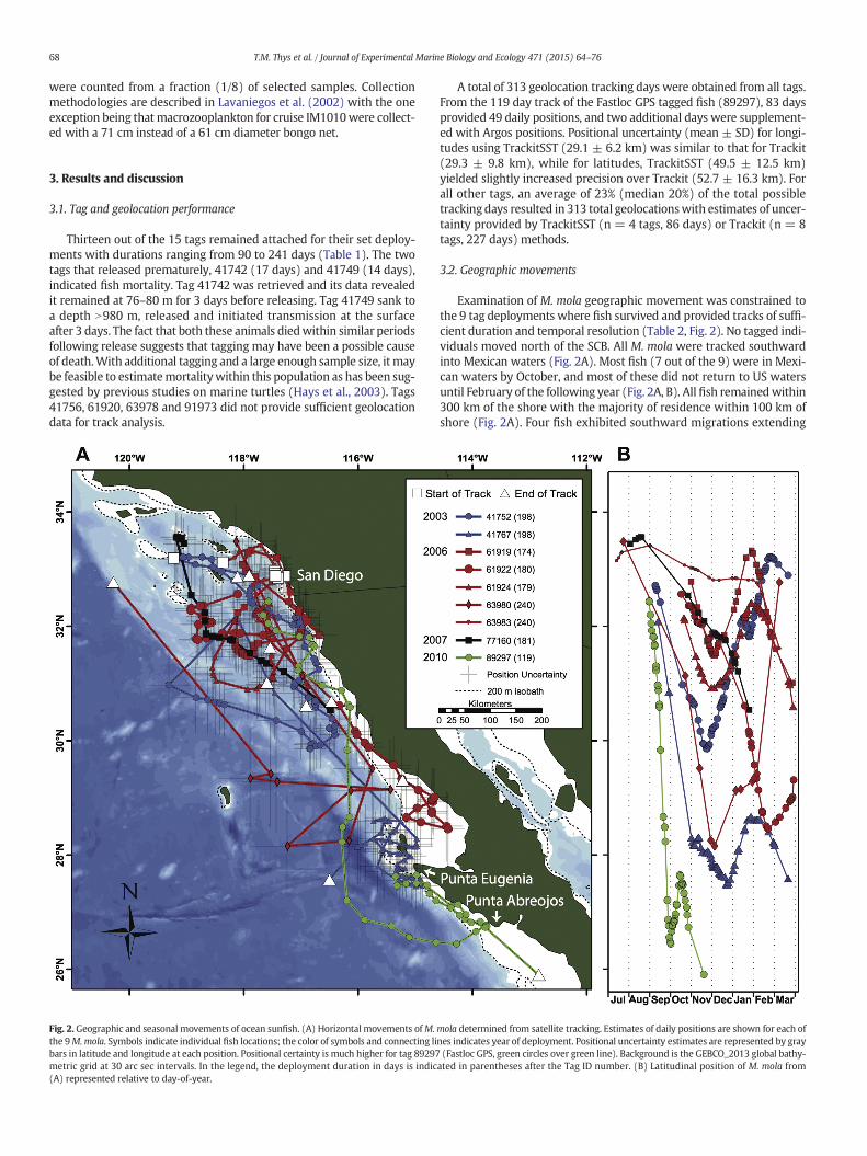
Fig. 2. Geographic and seasonal movements of ocean sunfish. (A) Horizontal movements ofM.the 9M.mola. Symbols indicate individual fish locations; the color of symbols and connecting libars in latitude and longitude at each position. Positional certainty is much higher for tag 89297metric grid at 30 arc sec intervals. In the legend, the deployment duration in days is indic(A) represented relative to day-of-year.

A total of 313 geolocation tracking days were obtained from all tags.From the 119 day track of the Fastloc GPS tagged fish (89297), 83 daysprovided 49 daily positions, and two additional days were supplement-ed with Argos positions. Positional uncertainty (mean ± SD) for longi-tudes using TrackitSST (29.1 ± 6.2 km) was similar to that for Trackit(29.3 ± 9.8 km), while for latitudes, TrackitSST (49.5 ± 12.5 km)yielded slightly increased precision over Trackit (52.7 ± 16.3 km). Forall other tags, an average of 23% (median 20%) of the total possibletracking days resulted in 313 total geolocationswith estimates of uncer-tainty provided by TrackitSST (n = 4 tags, 86 days) or Trackit (n = 8tags, 227 days) methods.

3.2. Geographic movements

Examination of M. mola geographic movement was constrained tothe 9 tag deployments where fish survived and provided tracks of suffi-cient duration and temporal resolution (Table 2, Fig. 2). No tagged indi-viduals moved north of the SCB. All M. mola were tracked southwardinto Mexican waters (Fig. 2A). Most fish (7 out of the 9) were in Mexi-can waters by October, and most of these did not return to US watersuntil February of the following year (Fig. 2A, B). All fish remainedwithin300 km of the shore with the majority of residence within 100 km ofshore (Fig. 2A). Four fish exhibited southward migrations extending

mola determined from satellite tracking. Estimates of daily positions are shown for each ofnes indicates year of deployment. Positional uncertainty estimates are represented by gray(Fastloc GPS, green circles over green line). Background is the GEBCO_2013 global bathy-

ated in parentheses after the Tag ID number. (B) Latitudinal position of M. mola from

40 20 0 20 40

0−55−1010−2525−5050−100100−150150−200200−300300−500

(m)

Percent of time in depth range

40 20 0 20 40

22−2420−2218−2016−1814−1612−1410−128−10< 8

( C)

Percent of time in temperature range

daynight

A B

Fig. 3.Depth and temperature range occupation of ocean sunfish. (A) Depth and (B) temperature histograms for day (white) and night (black) averaged for all fish in Table 2, except thosewith 12 and 24 h binning schemes and tag 77160, which used an alternate binning scheme. Data represent average percent time spent within each binned range.

69T.M. Thys et al. / Journal of Experimental Marine Biology and Ecology 471 (2015) 64–76

further than the others (tags 41767, 61922, 63980 and 89297). The far-thest and most rapid southward migration (~670 km in one month)was by the largest fish (tag 89297, 2 m TL), which was tracked as farsouth as Punta Abreojos, Baja California Sur. The extent and timing ofsouthward and northward movements were variable (Fig. 2B). Howev-er, 6 out of the 8 tagswith records N4months, reversed their southwardmovements to northward during the late fall and winter months of No-vember–December (Fig. 2B).

Horizontal movements were similar to those documented for otherM.mola long-term tagging studies: individuals tagged in coastal regionsdid not cross ocean basins but persistently inhabited the margins oftheir respective ocean basins (Dewar et al., 2010; Hays et al., 2009;Nakamura et al., 2015; Potter et al., 2011; Sims et al., 2009a,b). Paststudies report M. mola alternating between movement toward oraway from the equator, presumably to take advantage of greater pro-ductivity in spring and summer at higher latitudes (Parsons et al.,1984). For example, between spring and fall 2006, an ocean sunfishmi-grated 2619 km northeastward from coastal Japanese waters along thenorthwest Pacificmargin (Dewar et al., 2010).M.molamay alsomigrateto avoid cooler water temperatures. For example, as temperaturescooled between fall and winter 2005, an ocean sunfish migrated2520 km from New England waters southward into much warmer wa-ters around the Bahamas (Potter et al., 2011). A combination of produc-tivity and temperature likely drives these seasonal migrations.

117oW 116oW 115oW 114oW

26oN

27oN

28oN

29oN

117

120

123

127

130

50 km

Dep

th (

m)

0

50

100

150

Salini

33.5 3

BA

Fig. 4.Ocean sunfish depth occupation in relation to oxygendistributions. (A)Map of station loclights Line 127, which approached the coast within close range of theM. molamigration path (acquired between October 15, 10:00 and October 16, 03:00. The most inshore station was on thnorthward migration (October 3, 15:00–October 10, 17:00) and southward migration (Octobe

3.3. Southern CCLME depth and temperature preferences

M.mola occupied different depth and temperature ranges during theday versus night (Table 2, Fig. 3). This pattern is consistentwith diel ver-tical migrations (DVM), examples of which are presented for the FastlocGPS tag in Section 3.4. During the day, individuals frequented deeper,cooler waters with 59% of occupancy below 50 m. During the night,they were in shallower, warmer water with 97% of occupancy in theupper 50 m. Average maximum nighttime depth across all fish was59±9m (SE) compared to 174±8mduring the day. Correspondingly,the average minimum nighttime temperature was 13 ± 0.2 °C (SE)compared to 11 ± 0.2 °C during the day. Occasional deep dives(N500 m) were recorded for 4 M. mola, extending into temperaturesas cold as 6.6 °C (Table 2). Deep dives could be due to a variety of factorsas suggested by Houghton et al. (2008), including predator and shipevasion, thermoregulation and searching for prey. Ship evasion re-sponse could be explored in future studies by comparing deep dive loca-tions with geospatially matched automatic identification system (AIS)data collected by vessel traffic services (VTC) to identify and locate ves-sels. More detailed dive profile data than what was available in thisstudy is needed to explore any additional hypotheses.

Reasons underlying routine vertical movement have been linked toseveral factors. Vertical movement is likely used as a foraging strategyin search of patchily distributed prey as well as targeting the migration

ty

4 34.5

< 2.5

Oxygen (ml/L)

1 2 3 4 5 0 10 20 30

% of timeDC

ations occupied during IMECOCAL cruise IM1010, October 12–17, 2010. The gray line high-solid black circles). (B, C) Line 127 sections of salinity and dissolved oxygen concentration,e shelf (92 m). (D) Depth occupancy of theM. mola near the most inshore station duringr 24, 23:00–October 27, 14:00).

70 T.M. Thys et al. / Journal of Experimental Marine Biology and Ecology 471 (2015) 64–76

of the deep scattering layer (DSL) (Cartamil and Lowe, 2004; Dewaret al., 2010; Potter and Howell, 2011; Sims et al., 2009a,b). The bimodaldepth distribution during the day (Fig. 3) is consistent with repetitivedives between the mixed layer and the DSL. In Japanese waters,Nakamura et al. (2015) show M. mola surface to warm-up followingdives below the thermocline to the colder deep scattering layer.

Cartamil and Lowe (2004) also suggest that individuals in the SCBmay be recovering after frequenting depthswith decreased oxygen con-centrations. Ocean hypoxic zones (oxygen levels b2.5 ml l−1) arethought to induce avoidance responses in many fishes (Brill, 1994;Davis, 1975; Dewar et al., 2011). Over the past 30 years throughoutthe CCLME, the hypoxic boundary appears to be shoaling (Bogradet al., 2008). In this study, a cross-shelf section from the 2010IMECOCAL cruise approached, in space and time, the GPS trackedM. mola and thus allowed examination of potential impacts of dissolved

Fig. 5.Consistent association of a large sunfish (2m total length)with upwelling fronts. (A)Meanwith the period of tracking shown for Fastloc tag 89297. Boxes identify individual synoptic SSTinstantaneous, except for (C), which is a 1-day composite. Images B, C, F and H are from AVHRR;the range of variation within the domain; darker shades represent relatively coldwater associatcircles) are shown for available tracking datawithin±1.5 days of each image acquisition time. Inimage time (open black circle) during a 3-day window centered on the image time.

oxygen concentrations on M. mola vertical movements (Fig. 4A).Due to coastal upwelling, salinity and oxygen isopleths shoaled to-ward the coast (Fig. 4B, C). Low oxygen levels (b2.5 ml l−1) wererecorded b60 m below the surface at the most inshore station(Fig. 4C), and the water column structure suggests that these lowoxygen waters may have been even shallower closer to the coast.When the tagged individual was in the region of the inshore sta-tion, it spent 34% of its time below the shallow limit of the lowoxygen detected during the Line 127 survey (b2.5 ml l−1,Fig. 4D). These findings suggest that M. mola may be able to toler-ate low oxygen levels. Additional investigations into physiologicaltolerances of this species would be interesting, particularly in lightof recent reports of ocean oxygen minima expanding both in theSCB and globally as a result of climate change (McClatchie et al.,2010; Stramma et al., 2010).

sea surface temperature (SST) duringAugust 30 throughOctober 27, 2010, correspondingimage domains. (B–I) SST images from the domains labeled in (A). All images are nearlyimages D, E, G, and I are fromMODIS Aqua. In each image, gray scale shading is adapted toed with coastal upwelling. White scale bars in all images are 20 km.M.mola positions (redthe time reference atop each image, position times (solid red circles) are shown relative to

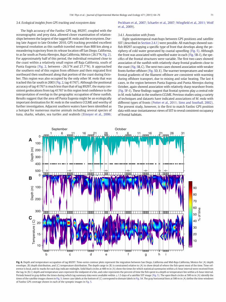
71T.M. Thys et al. / Journal of Experimental Marine Biology and Ecology 471 (2015) 64–76

3.4. Ecological insights from GPS tracking and ecosystem data

The high accuracy of the Fastloc GPS tag, 89297, coupled with theoceanographic and prey data, allowed closer examination of relation-ships between the largest of the taggedM.mola and the ecosystem.Dur-ing late August to late October 2010, GPS tracking provided excellenttemporal resolution as this sunfish traveled more than 800 km along ameandering trajectory from its release location off San Diego, California,to as far south as Punta Abreojos, Baja California,México (26.5°N, Fig. 2).For approximately half of this period, the individual remained close tothe coast within a relatively small region off Baja California, south ofPunta Eugenia (Fig. 2, between ~26.5°N and 27.7°N). It approachedthe southern end of this region from offshore and then migrated firstnorthward then southward along that portion of the coast during Octo-ber. This region was also occupied by the only other M. mola that wastracked this far south in 2003 (Fig. 2, tag 41767). Although thepositionalaccuracy of tag 41767 ismuch less than that of tag 89297, themany con-sistent geolocations from tag 41767 in this region lend confidence to theinterpretation of overlap in the geographic occupation of these sunfish.Results suggest that the area off Punta Eugenia might be an ecologicallyimportant destination forM.mola in the southern CCLME andworthy offurther investigation. Adjacent southern waters have been identified asa hotspot for numerous marine animals including several species oftuna, sharks, whales, sea turtles and seabirds (Etnoyer et al., 2006;

b c d e

0

100

200

300

400

500

Dep

th (

m)

1 6 11 16 21 26 1

Dep

th (

m)

0

100

200

300

Tem

pera

ture

(C

)

10

15

20

Septembe Or

A

B

C

Fig. 6. Depth and temperature occupation of tag 89297. Time-series contour plots represent thenvelope, (B) depth distribution, and (C) temperature distribution. The depth range in (B) is coerence is local, and ticmarks for each day indicatemidnight. Solid black circles at 400m in (A) sthe tag. In (B, C) depth and temperature axes represent themidpoint of a bin, and color represenPeriods boxed in gray define the times duringwhich tag summary datawere availablewithin±times of the satellite images shown in Fig. 5; lower case labels at the bottomof (C) correspond toof Fastloc GPS coverage shown in each of the synoptic images in Fig. 5.

Peckham et al., 2007; Schaefer et al., 2007; Wingfield et al., 2011; Wolfet al., 2009).

3.4.1. Association with frontsEight spatiotemporal matchups between GPS positions and satellite

SST (described in Section 2.4.1) were possible. All matchups showed sun-fish 89297 occupying a specific type of front that develops along the pe-riphery of cold water generated by coastal upwelling (Fig. 5). Althoughthe front was associatedwith upwelledwater in each (Fig. 5B–I), the spe-cifics of the frontal structures were variable. The first two cases showedassociation of the sunfish with relatively sharp frontal gradients close tothe coast (Fig. 5B, C). The next two cases showed associationwithweakerfronts further offshore (Fig. 5D, E). Thewarmer temperatures andweakerfrontal gradients of the filament offshore are consistent with warmingduring offshore transport, due to mixing and solar heating. The last 4cases, in the region between Punta Eugenia and Punta Abreojos duringOctober, again showed association with relatively sharp nearshore fronts(Fig. 5F–I). These findings suggest that frontal systems play a central roleinM.molahabitat in the southern CCLME. Previous studies using a varietyof techniques and datasets have indicated associations of M. mola withdifferent types of fronts (Potter et al., 2011; Sims and Southall, 2002).The present study, however, is the first to match Fastloc GPS positiondatawith near-instantaneous views of SST to reveal consistent occupancyof frontal habitats.

f g h i

6 11 16 21 26 31

% o

f tim

e

10

20

30

40

50

60

70

80

90

ctober

e migration between San Diego, California and Mid-Baja California, Mexico for (A) depthnstrained relative to (A) to show detail of where the fish spent most of the time. Time ref-how the times for which statistical summarieswithin a 6-hour interval were received fromts the percent of time the fish spent in a depth or temperature binwithin a 6-hour interval.1.5 days of a satellite SST image (Fig. 5). The open black circles at 500m in (A) identify thedomain labels in Fig. 5A. The gray horizontal lines at 500m in (A) define the timewindows

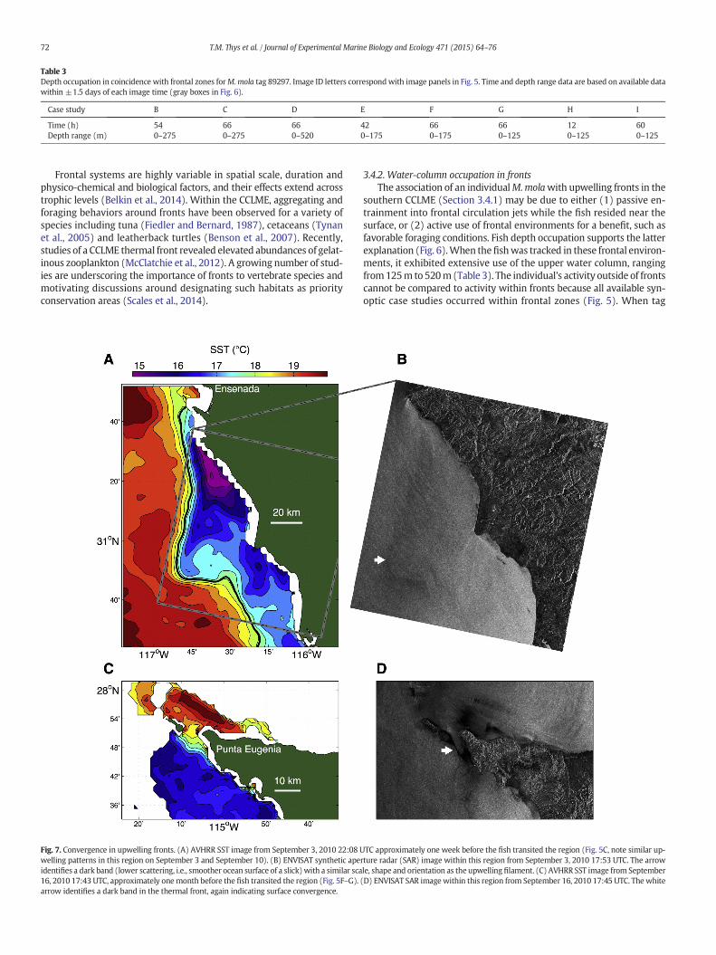
Table 3Depth occupation in coincidence with frontal zones forM.mola tag 89297. Image ID letters correspondwith image panels in Fig. 5. Time and depth range data are based on available datawithin ±1.5 days of each image time (gray boxes in Fig. 6).

Case study B C D E F G H I

Time (h) 54 66 66 42 66 66 12 60Depth range (m) 0–275 0–275 0–520 0–175 0–175 0–125 0–125 0–125

72 T.M. Thys et al. / Journal of Experimental Marine Biology and Ecology 471 (2015) 64–76

Frontal systems are highly variable in spatial scale, duration andphysico-chemical and biological factors, and their effects extend acrosstrophic levels (Belkin et al., 2014). Within the CCLME, aggregating andforaging behaviors around fronts have been observed for a variety ofspecies including tuna (Fiedler and Bernard, 1987), cetaceans (Tynanet al., 2005) and leatherback turtles (Benson et al., 2007). Recently,studies of a CCLME thermal front revealed elevated abundances of gelat-inous zooplankton (McClatchie et al., 2012). A growing number of stud-ies are underscoring the importance of fronts to vertebrate species andmotivating discussions around designating such habitats as priorityconservation areas (Scales et al., 2014).

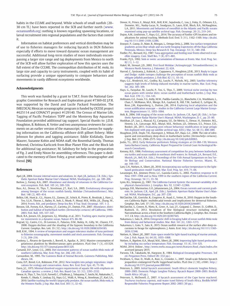
Fig. 7. Convergence in upwelling fronts. (A) AVHRR SST image from September 3, 2010 22:08 Uwelling patterns in this region on September 3 and September 10). (B) ENVISAT synthetic apeidentifies a dark band (lower scattering, i.e., smoother ocean surface of a slick)with a similar sca16, 2010 17:43 UTC, approximately onemonth before the fish transited the region (Fig. 5F–G).arrow identifies a dark band in the thermal front, again indicating surface convergence.

3.4.2. Water-column occupation in frontsThe association of an individualM.molawith upwelling fronts in the

southern CCLME (Section 3.4.1) may be due to either (1) passive en-trainment into frontal circulation jets while the fish resided near thesurface, or (2) active use of frontal environments for a benefit, such asfavorable foraging conditions. Fish depth occupation supports the latterexplanation (Fig. 6).When thefishwas tracked in these frontal environ-ments, it exhibited extensive use of the upper water column, rangingfrom125m to 520m (Table 3). The individual's activity outside of frontscannot be compared to activity within fronts because all available syn-optic case studies occurred within frontal zones (Fig. 5). When tag

TC approximately one week before the fish transited the region (Fig. 5C, note similar up-rture radar (SAR) image within this region from September 3, 2010 17:53 UTC. The arrowle, shape and orientation as the upwelling filament. (C) AVHRR SST image from September(D) ENVISAT SAR image within this region from September 16, 2010 17:45 UTC. The white

73T.M. Thys et al. / Journal of Experimental Marine Biology and Ecology 471 (2015) 64–76

data were of sufficient temporal resolution, diel vertical migration(DVM) was evident. Observations of DVM were clearly evidenced overtwo time periods: (1) between ~10 m (nighttime) and 40m (daytime)during September 1–4 (Fig. 6B), shortly after the fish was first associat-edwith a front (Fig. 5B), and (2) between ~20m (nighttime) and 200m(daytime) during September 20–24 (Fig. 6B, C), during and followingoccupation in a frontal zone furthest offshore (Fig. 5D). Considering allremote sensing case studies, DVMwas evident in depth and/or temper-ature data for cases c, d, g and i (Figs. 5, 6).

3.4.3. Frontal convergence zonesThe observed association of sunfish 89297 with upwelling fronts

(Fig. 5) motivated a more detailed investigation of the nature of thishabitat. Combined SAR and SST coverage during the tag tracking periodpermitted examination of two slicks in frontal zones. The first was fromthenorthern region of thefish track on September 3 (Fig. 7A, B), approx-imately one week before the fish transited the region (Fig. 5C). At thattime, a coastal upwelling plume extended ~50 km from the coast near31°N and was associated with strong thermal gradients (Fig. 7A). ASAR image acquired approximately 4 h before the SST image revealeda dark band having similar location and orientation as the upwellingfront (arrow in Fig. 7B). Dark bands indicate slicks typically associatedwith convergence zones (Holt, 2004; Ryan et al., 2010). Although advec-tion during the hours between the SAR and SST images precluded exactalignment of features in the SST and SAR images, the similarities of thethermal and surface roughness features support the interpretation of aconvergent thermal front. The second slick was from the southern re-gion of the track during mid-September (Fig. 7C, D), approximatelyone month before the fish transited the region (Fig. 5G). Nearly

Fig. 8. Zooplankton abundance in the region occupied for nearly one month by the largest tahydrocast stations; zooplankton was sampled at a subset of stations (pie charts). The pie charabundance. The dashed line is the 200 m isobath, representing the shelf break.

simultaneous SST and SAR images indicated a strong thermal front asso-ciated with coastal upwelling and an intense narrow slick in the frontalzone west of Punta Eugenia, Baja California (Fig. 7C, D).

The convergent circulation indicated by these two slicks has bothphysical and biological implications. When prey species swim upwardagainst the downwelling flow in a convergence, their populations canaccumulate (Franks, 1992). This mechanism can create favorable forag-ing habitats for predators such as M. mola.

3.4.4. Forage species in relation to frontsZooplankton sampling and environmental conditions within the

southern region of the fish's (89297) migration allows further explora-tion of the strong association between M. mola and upwelling fronts.The two highest zooplankton biovolumes were sampled near thecoast (Fig. 8, stations near 26.5°N and 28°N), where the sunfish spenthalf of the total two-month tracking period. Zooplankton biovolume atboth stations was dominated by salps, a known prey item for M. molaparticularly those N1 m (Cardona et al., 2012; Harrod et al., 2013;Nakamura and Sato, 2014; Syvaranta et al., 2012). In contrast, a near-coastal station sampled between these two high-abundance stationsshowed low biovolume (Fig. 8, station near 26.9°N). This difference inzooplankton biovolume was further related to frontal conditions. Atthe two near-coastal stations with high zooplankton biovolume, sam-pling occurred toward the warm side of strong thermal fronts (Fig. 9A,B, D). At the near-coastal stationwith low zooplankton biovolume, sam-pling occurred toward the cold side of a weaker thermal front (Fig. 9A,C). Although the zooplankton and environmental sampling were con-ducted on a prescribed grid, and thus not specifically designed to exam-ine relationships between zooplankton and fronts, the available data

gged M. mola (2 m TL, tag 89297, green line). Plus signs (+) mark the locations of shipt colors in the legend identify the dominant taxa in the two net tows having the greatest

−116 −115 −114

26

27

28

Longitude

Latit

ude

Temperature ( C)

16 17 18 19 20

−115.4−115.227.7

27.8

27.9

1718192021

C

−113.8

−113.6

26.426.526.626.7

17

18

19

20

21

C

−114.4 −114.2 −11426.7526.826.85

17

18

19

20

21

C

A

C

B

D

Fig. 9. Relationships between zooplankton abundance and fronts. (A) Near-surface (2 m) temperature along the ship track indicated by the + symbols in Fig. 8, which progressed fromnorth to south during October 12–17, 2010. (B–D) Temperature gradient plots representing the relationship between fronts and zooplankton biomass at the three nearshore stations (piecharts in Fig. 8); arrows define the location and temperature of the zooplankton sampling station.

74 T.M. Thys et al. / Journal of Experimental Marine Biology and Ecology 471 (2015) 64–76

support the interpretation that zooplankton biovolume was greater onthe warm side of strong thermal fronts. Studies in the northeastern At-lantic report findingM. mola on the warm stratified side of fronts, bothtidal and seasonal (Sims and Southall, 2002). The same may hold truefor M. mola in the southern CCLME.

3.4.5. Swimming speedsThe high accuracy and temporal intervals of the Fastloc GPS tag data

provided the opportunity to examine possible speed bursts of the large(2m TL) Fastloc tagged individual. Two unusually high speeds were de-tected during very short bursts. Each was based on GPS locations de-rived from 6 satellites at one location and 4 satellites at the other.Recent examination of Fastloc GPS accuracy shows that for positions cal-culated using 6 GPS satellites, 50% of locations were within 18 m, and95%werewithin 70m of the true position (Dujon et al., 2014). Accuracybased on 4 GPS satellites was lower, with 50% of locations within 36 m,and 95%were within 724 m of the true position. The speed estimate forthe first burst was 6.6 m s−1 during a 370 s interval with a correspond-ing error of ±0.15 (50% confidence) or ±2.1 (95% confidence). Thespeed estimate for the second burst was 2.2 m s−1 during a 342 s inter-val with a corresponding error of ±0.22 m s−1 (50% confidence) or±3.2 m s−1 (95% confidence). Given this positional uncertainty, we in-terpret the highest speed calculation, 6.6 ± 2.1 m s−1, with 95% confi-dence, as a reliable measure of a speed burst and not an outlier due tosampling or reporting error. Further, even with contribution to speedover ground from a strong flow in the California Current of ~0.5 m s−1

(Lynn and Simpson, 1987), this speed measurement remains anoma-lous. The uncertainty in the secondmeasurement exceeds the speed es-timate at the 95% confidence level and thus cannot be reliablyinterpreted as a speed burst. Nakamura and Sato (2014) report a

maximum burst speed of ~2.1 m s−1 for a smaller individual (1 m TL).Our estimate for maximum speed burst (6.6 m s−1) exceeds this by afactor of 3.

4. Conclusions

M. mola satellite telemetry studies in the southern CCLME between2003 and 2010 show that the species uses coastal ocean margins andengages in seasonal latitudinal movements extending between South-ern California and central Baja California, Mexico. Satellite and shipdata coupled with a high accuracy GPS track suggest that M. mola con-sistently occupy frontal zones where potential prey species such assalps may be concentrated. Further, ship measurements of oxygen pro-files show that aM.mola occupying near-coastal water likely spent timein hypoxic conditions. This observation motivates further physiologicalstudies of the species and tag-based oxygen measurements.

Studying individual M. mola offers valuable insight into the species'natural history and behavior in the eastern Pacific, yet important gapsstill remain in our understanding of the species' population ecology. On-going genetic surveys of the population coupledwith citizen science ob-servations (e.g. oceansunfish.org) and aerial and shipboard surveys thatrecord ocean sunfish sightings opportunistically (e.g. Barlow andForney, 2007; Benson et al., 2007) can help fill gaps. In the western At-lantic, such opportunistic ocean sunfish observations have been used toestimate summer abundances and establish a baseline for populationstatus assessments (Kenney, 1996). Similar work could be used to as-sess population status for the eastern Pacific M. mola population. Gapsalso remain in our understanding of ocean sunfish recruitment. Despitehigh fecundity, with an estimated 300 million eggs reported for a 1.2 mTL individual (Schmidt, 1921), no data exist on M. mola reproductive

75T.M. Thys et al. / Journal of Experimental Marine Biology and Ecology 471 (2015) 64–76

habits in the CCLME and beyond. While schools of small sunfish (20–30 cm TL) have been reported in the SCB and further north (www.oceansunfish.org) nothing is known regarding spawning locations, orlarval recruitment into regional populations and the factors that controlit.

Information on habitat preferences and vertical distribution may beof use to fisheries managers for reducing bycatch in DGN fisheriesespecially if efforts to move toward dynamic ocean management aresuccessful. Additional long-term studies of more individuals encom-passing a larger size range and tag deployments from Mexico to northof the SCB will allow further exploration of how this species uses thefull extent of the CCLME. The cosmopolitan distribution of M. mola, itslarge size and capacity to carry instruments, coupled with its habit ofsurfacing provide a unique opportunity to compare behaviors andmovements in vastly different ecosystems worldwide.

Acknowledgments

This work was funded by a grant to T.M.T. from the National Geo-graphic Committee for Research and Exploration grant #7369-02 J.P.R.was supported by the David and Lucile Packard Foundation. TheIMECOCALMexican oceanographic program is funded by CICESEproject#625114 and CONACYT project #129140. The Census of Marine Life,Tagging of Pacific Predators TOPP and the Monterey Bay AquariumFoundation provided additional tag support. Special thanks to: J.D.R.Houghton, B. Robison, R. Vetter and two anonymous reviewers for com-ments on an earlier version of the manuscript; Dan Lawson for supply-ing information on the California offshore drift gillnet fishery; MikeJohnson for photos and tagging assistance; Eddie Kisfaludy, DarenMaurer, Suzanne Kohin and NOAA staff, the Rosenthal family, ThomasBehrend, Christina Karliczek from Blue Planet Film and the Block labfor additional tag assistance; M. Salisbury for help in the preparationof Fig. 2 and Emily Nixon for assembling references. This paper is dedi-cated to the memory of Dave Foley, a great satellite oceanographer andfriend. [SS]

References

Apel, J.R., 2004. Oceanic internal waves and solutions. In: Apel, J.R., Jackson, C.R. (Eds.), Syn-thetic Aperture Radar Marine User's Manual. NOAA, Washington, D.C., pp. 189–206.

Barlow, J., Forney, K.A., 2007. Abundance and density of cetaceans in the California Cur-rent ecosystem. Fish. Bull. 105 (4), 509–526.

Bass, A.L., Dewar, H., Thys, T., Streelman, J.T., Karl, S.A., 2005. Evolutionary divergenceamong lineages of the ocean sunfish family, Molidae (Tetraodontiformes). Mar.Biol. 148 (2), 405–414.

Belkin, I.M., Hunt Jr., G.L., Hazen, E.L., Zamon, J.E., Schick, R., Prieto, R., Brodziak, J., Hare, J.,Teo, S.L.H., Thorne, L., Bailey, H., Itoh, S., Munk, P., Musyl, M.K., Willis, J.K., Zhang, W.,2014. Fronts, fish, and predators. Deep-Sea Res. II Top. Stud. Oceanogr. 107, 1–2.

Benson, S.R., Forney, K.A., Harvey, J.T., Carretta, J.V., Dutton, P.H., 2007. Abundance, distri-bution and habitat of leatherback turtles (Dermochelys coriacea) off California, 1990–2003. Fish. Bull. 105, 337–347.

Block, B.A., Jonsen, I.D., Jorgensen, S.J., Winship, et al., 2011. Tracking apex marine preda-tor movements in a dynamic ocean. Nature 475, 86–90.

Bograd, S.J., Castro, C.G., Di Lorenzo, E., Palacios, D.M., Bailey, H., Gilly, W., Chavez, F.P.,2008. Oxygen declines and the shoaling of the hypoxic boundary in the CaliforniaCurrent. Geophys. Res. Lett. 35 (12). http://dx.doi.org/10.1029/2008GL034185.

Brill, R.W., 1994. A review of temperature and oxygen tolerance studies of tuna pertinentto fisheries oceanography, movement models and stock assessments. Fish. Oceanogr.3 (3), 204–216.

Cardona, L., Álvarez de Quevedo, I., Borrell, A., Aguilar, A., 2012. Massive consumption ofgelatinous plankton by Mediterranean apex predators. PLoS One 7 (3), e31329.http://dx.doi.org/10.1371/journal.pone.0031329.

Cartamil, D.P., Lowe, C.G., 2004. Diel movement patterns of ocean sunfish Mola mola offsouthern California. Mar. Ecol. Prog. Ser. 266, 245–253.

Carwardine, M., 1995. The Guinness Book of Animal Records. Guinness Publishing, Mid-dlesex, UK.

Costa, D.P., Breed, G.A., Robinson, P.W., 2012. New insights into pelagic migrations: impli-cations for ecology and conservation. Annu. Rev. Ecol. Evol. Syst. 43, 73–96.

Davis, J.C., 1975. Minimal dissolved oxygen requirements of aquatic life with emphasis onCanadian species: a review. J. Fish. Res. Board Can. 32 (12), 2295–2332.

Dewar, H., Thys, T., Teo, S.L.H., Farwell, C., O'Sullivan, J., Tobayama, T., Soichi,M., Nakatsubo, T.,Kondo, Y., Okada, Y., Lindsay, D.J., Hays, G.C., Walli, A., Weng, K., Streelman, J.T., Karl, S.A.,2010. Satellite tracking theworld's largest jelly predator, the ocean sunfish,Molamola, inthe Western Pacific. J. Exp. Mar. Biol. Ecol. 393 (1), 32–42.

Dewar, H., Prince, E., Musyl, M.K., Brill, R.W., Sepulveda, C., Lou, J., Foley, D., Orbesen, E.S.,Domeier, M.L., Nasby-Lucas, N., Snodgrass, D., Laurs, R.M., Block, B.A., McNaughton,L.A., 2011. Movements and behaviors of swordfish in the Atlantic and Pacific oceansexamined using pop-up satellite archival tags. Fish. Oceanogr. 20 (3), 219–241.

Dujon, A.M., Lindstrom, T., Hays, G.C., 2014. The accuracy of Fastloc-GPS locations and im-plications for animal tracking. Methods Ecol. Evol. 5 (11), 1162–1169. http://dx.doi.org/10.1111/2041-210X.12286.

Etnoyer, P., Canny, D., Mate, B., Morgan, L., Ortega-Ortiz, J., 2006. Sea-surface temperaturegradients across blue whale and sea turtle foraging trajectories off the Baja CaliforniaPeninsula, Mexico. Deep-Sea Research II. Top. Oceanogr. 53 (3), 340–358.

Fiedler, P.C., Bernard, H.J., 1987. Tuna aggregation and feeding near fronts observed in sat-ellite imagery. Cont. Shelf Res. 7 (8), 871–881.

Franks, P.J.S., 1992. Sink or swim: accumulation of biomass at fronts. Mar. Ecol. Prog. Ser.82 (1), 1–12.

Hakel, M., Stewart, J.D., 2002. First fossil Molidae (Actinopterygii: Tetraodontiformes) inWestern North America. J. Paleontol. 22, 62A.

Harrod, C., Syväranta, J., Kubicek, L., Cappanera, V., Houghton, J.D.R., 2013. Reply to Loganand Dodge: stable isotopes challenge the perception of ocean sunfish Mola mola asobligate jellyfish predators. J. Fish Biol. 82 (1), 10–16.

Hays, G.C., Broderick, A.C., Godley, B.J., Luschi, P., Nichols, W.J., 2003. Satellite telemetrysuggests high levels of fishing-induced mortality in marine turtles. Mar. Ecol. Prog.Ser. 262, 305–309.

Hays, G., Farquhar, M., Luschi, P., Teo, S., Thys, T., 2009. Vertical niche overlap by twoocean giants with similar diets: ocean sunfish and leatherback turtles. J. Exp. Mar.Biol. Ecol. 370 (1), 134–143.

Hofmann, G.E., Evans, T.G., Kelly, M.W., Padilla-Gamiño, J.L., Blanchette, C.A., Washburn, L.,Chan, F., McManus, M.A., Menge, B.A., Gaylord, B., Hill, T.M., Sanford, E., LaVigne, M.,Rose, J.M., Kapsenberg, L., Dutton, J.M., 2014. Exploring local adaptation and theocean acidification seascape — studies in the California Current Large Marine Ecosys-tem. Biogeosciences 11, 1053–1064.

Holt, B., 2004. SAR imaging of the ocean surface. In: Jackson, C.R., Apel, J.R. (Eds.), in Syn-thetic Aperture Radar Marine User's Manual. NOAA, Washington, D. C., pp. 25–80.

Hoolihan, J.P., Luo, J., Abascal, F.J., Campana, S.E., De Metrio, G., Dewar, H., Domeier, M.L.,Howey, L.A., Lutcavage, M.E., Musyl, M.K., Neilson, J.D., Orbesen, E.S., Prince, E.D.,Rooker, J.R., 2011. Evaluating post-release behaviour modification in large pelagicfish deployed with pop-up satellite archival tags. ICES J. Mar. Sci. 68 (5), 880–889.

Houghton, J.D.R., Doyle, T.K., Davenport, J., Wilson, R.P., Hays, G.C., 2008. The role of infre-quent and extraordinary deep dives in leatherback turtles (Dermochelys coriacea).J. Exp. Biol. 211, 2566–2575. http://dx.doi.org/10.1242/jeb.020065.

Joslin, T.L., 2012. Early Holocene prehistoric fishing strategies at CA-SBA-139, WesternSanta Barbara County, California. Report Prepared for Central Coast Archeological Re-search Consultants.

Kenney, R.D., 1996. Preliminary assessment of competition for prey between leatherbacksea turtles and ocean sunfish in northeast shelf waters. In: Keinath, J.A., Bernard, D.E.,Musick, J.A., Bell, B.A. (Eds.), Proceedings of the 15th Annual Symposium on Sea Tur-tle Biology and Conservation. National Marine Fisheries Service, Miami, FL,pp. 144–147.

Lam, C.H., Nielsen, A., Sibert, J.R., 2010. Incorporating sea-surface temperature to the light-based geolocation model TrackIt. Mar. Ecol. Prog. Ser. 419, 71–84.

Lavaniegos, B.E., Jimenez-Perez, L.C., Gaxiola-Castro, G., 2002. Plankton response to ElNino 1997–1998 and La Nina 1999 in the southern region of the California Current.Prog. Oceanogr. 54 (1), 33–58.

Lynn, R.L., Simpson, J.J., 1987. The California Current System: the seasonal variability of itsphysical characteristics. J. Geophys. Res. 92, 12,947–12,966.

Lyzenga, D.R., Marmorino, G.O., Johannessen, J.A., 2004. Ocean currents and current gradi-ents. In: Jackson, C.R., Apel, J.R. (Eds.), Synthetic Aperture Radar Marine User's Man-ual. NOAA, Washington, D.C., pp. 207–220.

McClatchie, S.R., Goericke, R., Cosgrove, R., Auad, G., Vetter, R., 2010. Oxygen in the South-ern California Bight: multidecadal trends and implications for demersal fisheries.Geophys. Res. Lett. 37 (19). http://dx.doi.org/10.1029/2010GL044497.

McClatchie, S., Cowen, R., Nieto, K., Greer, A., Luo, J.Y., Guigand, C., Demer, D., Griffith, D.,Rudnick, D., 2012. Resolution of fine biological structure including smallNarcomedusae across a front in the Southern California Bight. J. Geophys. Res. Oceans117, C4. http://dx.doi.org/10.1029/2011JC007565.

Nakamura, I., Sato, K., 2014. Ontogenetic shift in foraging habit of ocean sunfishMolamolafrom dietary and behavioral studies. Mar. Biol. 161 (6), 1263–1273.

Nakamura, I., Goto, Y., Sato, K., 2015. Ocean sunfish rewarm at the surface after deep ex-cursions to forage for siphonophores. J. Anim. Ecol. http://dx.doi.org/10.1111/1365-2656.12346.

Nielsen, A., Sibert, J.R., 2007. State-spacemodel for light-based tracking of marine animals.Can. J. Fish. Aquat. Sci. 64 (8), 1055–1068.

Nielsen, A., Bigelow, K.A., Musyl, M.K., Sibert, J.R., 2006. Improving light-based geolocationby including sea surface temperature. Fish. Oceanogr. 15 (4), 314–325.

NOAA, 2014. Online:, http://www.nwfsc.noaa.gov/news/features/food_chain/index.cfmaccessed January 2015.

Parsons, T.R., Takahashi, M., Hargrave, B., 1984. Biological Oceanographic Processes. 3rded. Pergamon Press, Oxford UK (332 pp.).

Peckham, S., Diaz, D., Walli, A., Ruiz, G., Crowder, L., 2007. Small-scale fisheries bycatchjeopardizes endangered Pacific loggerhead turtles. PLoS One 2 (10), e1041. http://dx.doi.org/10.1371/journal.pone.0001041.

Petersen, S., 2005. Initial bycatch assessment: South Africa's domestic longline fishery,2000–2003. Domestic Pelagic Longline Fishery: Bycatch Report 2000–2003. BirdLifeSouth Africa (45 pp.).

Petersen, S., McDonell, Z., 2007. A bycatch assessment of the Cape horse mackerel,Trachurus trachurus capensis, mid-water trawl fishery of South Africa. Birdlife/WWFResponsible Fisheries Programme Report 2002–2003 (30 pp.).

76 T.M. Thys et al. / Journal of Experimental Marine Biology and Ecology 471 (2015) 64–76

Pope, E., Hays, G., Thys, T., Doyle, T., Sims, D., Queiroz, N., Hobson, V., Kubicek, L.,Houghton, J.D.R., 2010. The biology and ecology of the ocean sunfishMola mola: a re-view of current knowledge and future research perspectives. Rev. Fish Biol. Fish. 20(4), 471–487. http://dx.doi.org/10.1007/s11160-009-9155-9.

Porcasi, J.F., Andrews, S.L., 2001. Evidence for a prehistoric Mola mola fishery on theSouthern California coast. J. Calif. Great Basin Anthropol. 23 (1), 51–66.

Potter, I.F., Howell, W.H., 2011. Vertical movements and behavior of the ocean sunfish,Mola mola, in the Northwest Atlantic. J. Exp. Mar. Biol. Ecol. 396 (2), 138–146.

Potter, I.F., Galuardi, B., Howell, W.H., 2011. Horizontal movement of ocean sunfish, Molamola, in the Northwest Atlantic. Mar. Biol. 158 (3), 531–540.

R Development Core Team, 2013. R: A Language and Environment for Statistical Comput-ing. R Foundation for Statistical Computing, Vienna (www.r-project.org/. Retrieved23 July 2013).

Roach, J., 2003. World's Heaviest Bony Fish Discovered? National Geographic (news.nationalgeographic.com/news/2003/05/0513_030513_sunfish.html. accessed 23July 2013)

Ryan, J.P., Fischer, A.M., Kudela, R.M., McManus, M.A., Myers, J.S., Paduan, J.D., Ruhsam, C.M.,Woodson, C.B., Zhang, Y., 2010. Recurrent frontal slicks of a coastal ocean upwellingshadow. J. Geophys. Res. Oceans 115, C12. http://dx.doi.org/10.1029/2010JC006398.

Ryan, J.P., Dierssen, H.M., Kudela, R.M., Scholin, C.A., Johnson, K.S., Sullivan, J.M., Fischer,A.M., Rienecker, E.V., McEnaney, P.R., Chavez, F.P., 2005. Coastal ocean physics andred tides, an example from Monterey Bay, California. Oceanography 18, 246–255.

Ryan, J.P., McManus, M.A., Paduan, J.D., Chavez, F.P., 2008. Phytoplankton thin layers with-in coastal upwelling system fronts. Mar. Ecol. Prog. Ser. 354, 21–34. http://dx.doi.org/10.3354/meps07222.

Sawai, E., Yamanoue, Y., Yoshita, Y., Sakai, Y., Hashimoto, H., 2011. Seasonal occurrencepatterns of Mola sunfishes (Mola spp. A and B; Molidae) in waters off the Sanriku re-gion, eastern Japan. Japn. J. Ichthyol. 58 (2), 181–187.

Scales, K.L., Miller, P.I., Hawkes, L.A., Ingram, S.N., Sims, D.W., Votier, S.C., 2014. On thefront line: frontal zones as priority at-sea conservation areas frommobilemarine ver-tebrates. J. Appl. Ecol. 51 (6), 1575–1583. http://dx.doi.org/10.1111/1365-2664.12330.

Schaefer, K., Fuller, D., Block, B., 2007. Movements, behavior, and habitat utilization ofyellowfin tuna (Thunnus albacares) in the northeastern Pacific Ocean, ascertainedthrough archival tag data. Mar. Biol. 152 (3), 503–525.

Schmidt, J., 1921. New studies of sun-fishes made during the “Dana” Expedition, 1920.Nature 107, 76–79.

Silvani, L., Gazo, M., Aguilar, A., 1999. Spanish driftnet fishing and incidental catches in thewestern Mediterranean. Biol. Conserv. 90 (1), 79–85.

Sims, D.W., Southall, E.J., 2002. Occurrence of ocean sunfish,Mola mola, near fronts in thewestern English Channel. J. Mar. Biol. Assoc. UK 82 (5), 927–928.

Sims, D.W., Queiroz, N., Doyle, T.K., Houghton, J.D.R., Hayes, G., 2009a. Satellite tracking ofthe world's largest bony fish, the ocean sunfish (Mola mola) in the North East Atlan-tic. J. Exp. Mar. Biol. Ecol. 370 (1), 127–133.

Sims, D.W., Queiroz, N., Humphries, N., Lima, F., Hays, G., 2009b. Long-term GPS trackingof ocean sunfish, Mola mola, offers a new direction in fish monitoring. PLoS One 4(10), e7351. http://dx.doi.org/10.1371/ journal.pone.0007351.

Stramma, L., Schmidtko, S., Levin, L., Johnson, G., 2010. Ocean oxygen minima expansionsand their biological impacts. Deep-Sea Res. I Oceanogr. Res. Pap. 57 (4), 587–595.

Syvaranta, J., Harrod, C., Kubicek, L., Cappanera, V., Houghton, J.D.R., 2012. Stable isotopeschallenge the perception of ocean sunfish Mola mola as obligate jellyfish predators.J. Fish Biol. 80 (1), 225–231.

Tudela, S., Kai Kai, A., Maynou, F., El Andalossi, M., Guglielmi, P., 2005. Driftnet fishing andbiodiversity conservation: the case study of the large-scale Moroccan driftnet fleetoperating in the Alboran Sea (SW Mediterranean). Biol. Conserv. 121 (1), 65–78.

Tynan, C.T., Ainley, D.G., Barth, J.A., Cowles, T.J., Pierce, S.D., Spear, L.B., 2005. Cetacean dis-tributions relative to ocean processes in the northern California Current System.Deep-Sea Res. II Top. Stud. Oceanogr. 52 (1), 145–167.

Watanabe, Y., Sato, K., 2008. Functional dorsoventral symmetry in relation to lift-basedswimming in the ocean sunfish Mola mola. PLoS One 3 e3446.

Wingfield, D.K., Peckham, S.H., Foley, D.G., Palacios, D.M., Lavaniegos, B.E., Durazo, R.,Nichols, W.J., Croll, D.A., Bograd, S.J., 2011. The making of a productivity hotspot inthe coastal ocean. PLoS One 6 (11), e27874.

Wolf, S., Sydeman, W., Hipfner, J., Abraham, C., Tershy, B., 2009. Range-wide reproductiveconsequences of ocean climate variability for the seabird, Cassin's Auklet. Ecology 90(3), 742–753.

Yoshita, Y., Yamanoue, Y., Sagara, K., Nishibori, M., Kuniyoshi, H., Umino, T., Sakai, Y.,Hashimoto, H., Gushima, K., 2009. Phylogenetic relationship of two Mola sunfishes(Tetraodontiformes: Molidae) occurring around the coast of Japan, with notes ontheir geographical distribution and morphological characteristics. Ichthyol. Res. 56(3), 232–244. http://dx.doi.org/10.1007/s10228-008-0089-3.

Further Reading

www.argos-system.org/manual/3-location/34_location_classes.html (Retrieved January2, 2015).

www.westcoast.fisheries.noaa.gov/fisheries/wc_oberserver_program_info/data_summ_report_sw_observer_fish.html (Retrieved January 2 2015).