Journal of Economics and Business 71 (2014) 68– 89

Contents lists available at ScienceDirect

Journal of Economics and Business

Portfolio optimization in an upside potentialand downside risk framework�

Denisa Cumovaa, David Nawrockib,∗

a Berenberg Bank, Neuer Jungfernstieg 20, 20354 Hamburg, Germanyb Villanova University, Department of Finance, Villanova School of Business, 800 Lancaster Avenue,Villanova, PA 19085, USA

a r t i c l e i n f o

Article history:Received 12 January 2011Received in revised form 11 July 2013Accepted 12 August 2013

Keywords:Portfolio optimizationVon Neumann and Morganstern utilitytheoryLower partial moment and upper partialmoment optimization formulationFour utility cases

a b s t r a c t

The lower partial moment (LPM) has been the downside risk mea-sure that is most commonly used in portfolio analysis. Its majordisadvantage is that its underlying utility functions are linearabove some target return. As a result, the upper partial moment(UPM)/lower partial moment (LPM) analysis has been suggestedby Holthausen (1981. American Economic Review, v71(1), 182), Kanget al. (1996. Journal of Economics and Business, v48, 47), and Sortinoet al. (1999. Journal of Portfolio Management, v26(1,Fall), 50) as amethod of dealing with investor utility above the target return.Unfortunately, they only provide dominance rules rather than aportfolio selection methodology. This paper proposes a formulationof the UPM/LPM portfolio selection model and presents four utilitycase studies to illustrate its ability to generate a concave efficientfrontier in the appropriate UPM/LPM space. This framework imple-ments the full richness of economic utility theory be it [Friedmanand Savage (1948). Journal of Political Economy, 56, 279; Markowitz,H. (1952). Journal of Political Economy, 60(2), 151; Von Neumann, J.,& Morgenstern, O. (1944). Theory of games and economic behavior.(3rd ed., 1953), Princeton University Press], and the prospect theoryof (Kahneman and Tversky (1979). Econometrica, 47(2), 263).

� The authors would like to thank D. Hillier, S. Brown, J. Estrada, T. Post, P. Van Vliet, F. Viole, anonymous referees and theFinance Seminar Series at Villanova University for their comments on earlier versions of this paper. All errors of course are theresponsibility of the authors.

∗ Corresponding author. Tel.: +1 610 519 4323.E-mail addresses: Denisa.Cumova@berenbergbank.de (D. Cumova), david.nawrocki@villanova.edu (D. Nawrocki).

0148-6195/$ – see front matter © 2013 Elsevier Inc. All rights reserved.http://dx.doi.org/10.1016/j.jeconbus.2013.08.001

D. Cumova, D. Nawrocki / Journal of Economics and Business 71 (2014) 68– 89 69

The methods and techniques proposed in this paper are focused onthe following computational issues with UPM/LPM optimization.

• Lack of positive semi-definite UPM and LPM matrices.• Rank of matrix errors.• Estimation errors.• Endogenous and exogenous UPM and LPM matrices.

© 2013 Elsevier Inc. All rights reserved.

1. Introduction

The mean-lower partial moment (�,LPM) model has been attractive to decision makers becauseit does not require any distributional assumptions and it is a necessary and sufficient condition forinvestors with various classes of Von Neumann and Morgenstern (1944) (hereafter, vNM) utility func-tions which is equivalent to expected utility-maximization under risk aversion.1 Because it does notmake any distributional assumption, it has been particularly useful in the management of derivativeportfolios (Merriken, 1994; Huang, Srivastava, & Raatz, 2001; Pedersen, 2001; and Jarrow & Zhao,2006).

However, LPM has traditionally been challenged by academic researchers because of the com-putational complexity of the asymmetric Co-LPM matrix used in �-LPM portfolio analysis and thepersistent belief that it is an ad-hoc method that is not grounded in capital market equilibrium theoryand in expected utility maximization theory.2

A major challenge to the use of any portfolio theory formulation that does not use mean-varianceanalysis is by Markowitz (2010). His position is even with non-normal security distributions, the mean-variance criterion is still a useful approximation of the expected utility of the investor. In other words,any alternative to mean-variance portfolio theory has to rest on a solid foundation of utility theory.It is not sufficient for the portfolio framework to simply be a nonparametric approach. The UPM/LPMframework is powerful because it is a nonparametric approach and it implements the full richnessof economic utility theory be it Friedman and Savage (1948), Markowitz (1952), Von Neumann andMorgenstern (1944), or the prospect theory of Kahneman and Tversky (1979). Markowitz (2010) doesend up supporting the geometric mean-semivariance portfolio theory model in his paper because of itsutility theory foundation. Semivariance is the only risk measure other than variance that is accordedany support by Markowitz (1959, 2010).

While our focus is not on LPM and capital market theory, the discussion in Hogan and Warren(1974), Bawa and Lindenberg (1977), Harlow and Rao (1989), Leland (1999), and Pedersen and Satchell(2002) makes it pretty clear that LPM is not an ad-hoc model that is ungrounded in capital markettheory. We are interested in solving the computational complexities of the �-LPM and its well-knownutility maximization limitation of assuming a linear utility function above the target return.3 By solvingthe �-LPM computational problem, we are able to introduce the upper partial moment-lower par-tial moment (UPM/LPM) portfolio selection model which extends the expected utility maximizationcapabilities of the LPM model.

The paper continues with a discussion of mean-LPM and UPM/LPM portfolio analysis and theirplace in expected utility theory. Next, we offer a formulation for testing UPM/LPM portfolio opti-mization problems and discuss the historic issue of exogenous and endogenous LPM matrices. Next,four empirical problems are discussed which include: (1) Lack of positive semi-definite UPM and LPMmatrices; (2) Rank of matrix errors; (3) Estimation errors; and (4) Endogenous and Exogenous UPM

1 See Frowein (2000) for the necessary and sufficient conditions.2 See Grootveld and Hallerbach (1999) for a discussion of empirical issues and Pedersen and Satchell (2002) for a discussion

of the theoretical foundation of �-LPM in capital market theory.3 LPM utility functions are interested only in downside or below target return risk. It assumes a risk-neutral investor for

above-target returns. See Fishburn (1977), Fishburn and Kochenberger (1979) and Kaplan and Siegel (1994a, 1994b).

70 D. Cumova, D. Nawrocki / Journal of Economics and Business 71 (2014) 68– 89

and LPM matrices. The paper offers discussions and solutions for each of these problems. Finally, thepaper will present four utility theory case problems to illustrate the ability of the UPM/LPM model togenerate a concave efficient frontier in the appropriate UPM/LPM space.

2. UPM/LPM, stochastic dominance and expected utility maximization

Stochastic dominance is the analysis of the cumulative probability function of two securities andis used to determine investor preference for one asset over the other. Bawa (1975) provided proofsthat in terms of expected utility theory, first degree stochastic dominance (FSD) contains all utilityfunctions, second degree stochastic dominance (SSD) contains all risk averse utility functions and thirddegree stochastic dominance (TSD) includes all utility functions with decreasing absolute risk averseutility functions.4

The foundation of the congruence of LPM with expected utility maximization goes back to Porter(1974) who found that the SSD set contains all mean-semivariance (from a target return) dominantportfolios.

In terms of stochastic dominance, Bawa (1975) shows that the mean-variance is neither anecessary nor a sufficient condition for SSD and that mean-variance is consistent with VonNeumann–Morgenstern utility theory only if the utility function is quadratic.5 By contrast, the TSDadmissible set contains all mean-target semivariance (LPM degree 2) rules. Therefore, Bawa concludesthat mean-semivariance can be used as a suitable approximation to the TSD rule.6

Fishburn extends Bawa’s analysis to his Theorem 3 that states that the LPM is a family of utilityfunctions denoted by the LPM degree a such that:

FSD contains all mean-LPM(a,t) decision rules for all a ≥ 0.SSD contains all mean-LPM(a,t) decision rules for all a ≥ 1.TSD contains all mean-LPM(a,t) decision rules for all a ≥ 2.

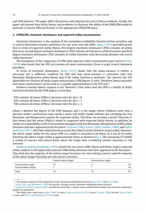
where a denotes the degree of the LPM measure and t is the target return. Fishburn notes that adecision maker’s preferences may satisfy a mean-risk utility model without also satisfying the VonNeumann and Morgenstern axioms for expected utility. Therefore, he provides a proof (Theorem 2)that shows that the mean-LPM(a,t) model is congruent with expected utility theory. In addition, hestudies its compatibility with 24 investment managers with Von Neumann–Morgenstern (vNM) utilityfunctions that have appeared in the literature: Grayson (1960), Green (1963), Swalm (1966), and Halterand Dean (1971). All of the utility functions can be described in terms of below-target utility. However,the above target utility for the mean-LPM (a,t) model is assumed to be linear. In 9 out of 24 utilityfunctions the above-target utility is approximately linear as shown in Fig. 1. The remaining 15 exhibita variety of concave and convex forms above the target with a tendency toward concavity or riskaversion.

Fishburn and Kochenberger (1979) extend the two-piece vNM (above and below target) expectedutility analysis to 28 empirically assessed vNM utility functions that have appeared in the literature.7

They find that the majority of the below-target functions are risk seeking (convex) and the majorityof the above-target functions are risk averse (concave).

Concave above target Convex above target

Convex below target 13 5 18Concave below target 3 7 10

Total 16 12 28

4 The analysis consists of the integration of the cumulative probability function Bawa (1975) and Levy (1998).5 Kroll, Levy, and Markowitz (1984) do provide a strong counter-argument supporting mean-variance.6 Ogryczak and Ruszczynski (2001) provide the proof that n-degree mean-semideviation models and stochastic dominance

models are equivalent.7 The utility cases came from Swalm (1966) 13 cases, Halter and Dean (1971) 2 cases, Grayson (1960) 8 cases, Green (1963)

3 cases, and Barnes and Reinmuth (1976) 2 cases.

D. Cumova, D. Nawrocki / Journal of Economics and Business 71 (2014) 68– 89 71

Fig. 1. Plots of LPM utility functions for five values of a = 0, 1/2, 1, 2, and 4. Note that all utility functions are linear above thetarget return t. Source: Fishburn (1977).

The finding of convex–concave and concave–convex utility functions in more than 70% of the casessupports the Kahneman and Tversky (1979) reflection effect, which suggests that above-target riskaversion is often accompanied by below-target risk seeking and above-target risk seeking is oftenaccompanied by below-target risk aversion.8 In these reported utility cases, (only 3 of 28), the frequentlyinvoked assumption that individuals are everywhere risk averse (concave–concave) does not hold.

Holthausen (1981), looking at Fishburn’s �-LPM(a,t) results, wonders why the criteria should con-tinue to use the expected mean which includes all returns from below the target. This is redundantbecause the downside returns are already included in the LPM(a,t) calculation.9 Another concern isthat the mean-LPM(a,t) model imposes risk neutrality above the target return. Given the results fromFishburn (1977) and Fishburn and Kochenberger (1979) showing linear, convex and concave func-tions above the target, Holthausen proposes the a–ˇ–t model, or upper partial moment/lower partialmoment (UPM/LPM) model where ̌ is the coefficient for the above-target utility (see Fig. 2). Investorscan be classified as risk seeking (a < 1, ̌ > 1), risk neutral (a = 1, ̌ = 1) and risk averse (a > 1, ̌ < 1). Hedemonstrates that this model is congruent with expected utility theory.

Holthausen (1981) provides a proof for the following relationships:

FSD contains all UPM/LPM(a,ˇ,t) rules for all a ≥ 0, ̌ ≥ 0.SSD contains all UPM/LPM(a,ˇ,t) rules for all a ≥ 1, 0 ≤ ̌ ≤ 1.TSD contains all UPM/LPM(a,ˇ,t) rules for all a ≥ 2, 0 ≤ ̌ ≤ 1.

8 We propose that upside risk seeking and upside risk aversion are more appropriately denoted as “potential seeking” and“potential averse”. These terms more accurately describe the upside behavior of investors.

9 We can give you a simple example why UPM/LPM is important. Let’s assume that the target return is 3%. Now, a 2% returnwill enter the LPM calculation as a below-target return. It will also enter into the calculation of the mean return. So whencomputing a mean/LPM ratio, that particular return is being counted twice, both in the numerator and the denominator, andit represents a positive outcome in the mean calculation and a negative outcome in the LPM calculation. UPM/LPM analysisavoids this conflict Musiol and Muhlig (2003).

72 D. Cumova, D. Nawrocki / Journal of Economics and Business 71 (2014) 68– 89

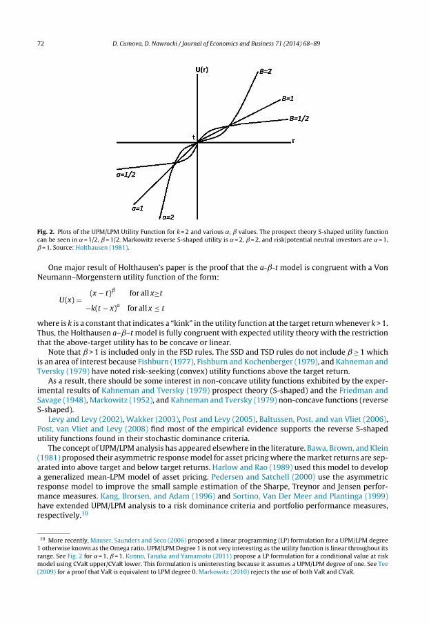
Fig. 2. Plots of the UPM/LPM Utility Function for k = 2 and various ˛, ̌ values. The prospect theory S-shaped utility functioncan be seen in ̨ = 1/2, ̌ = 1/2. Markowitz reverse S-shaped utility is ̨ = 2, ̌ = 2, and risk/potential neutral investors are ̨ = 1,ˇ = 1. Source: Holthausen (1981).

One major result of Holthausen’s paper is the proof that the a-ˇ-t model is congruent with a VonNeumann–Morgenstern utility function of the form:

U(x) =(x − t)ˇ for all x≥t

−k(t − x)a for all x ≤ t

where is k is a constant that indicates a “kink” in the utility function at the target return whenever k > 1.Thus, the Holthausen a–ˇ–t model is fully congruent with expected utility theory with the restrictionthat the above-target utility has to be concave or linear.

Note that ̌ > 1 is included only in the FSD rules. The SSD and TSD rules do not include ̌ ≥ 1 whichis an area of interest because Fishburn (1977), Fishburn and Kochenberger (1979), and Kahneman andTversky (1979) have noted risk-seeking (convex) utility functions above the target return.

As a result, there should be some interest in non-concave utility functions exhibited by the exper-imental results of Kahneman and Tversky (1979) prospect theory (S-shaped) and the Friedman andSavage (1948), Markowitz (1952), and Kahneman and Tversky (1979) non-concave functions (reverseS-shaped).

Levy and Levy (2002), Wakker (2003), Post and Levy (2005), Baltussen, Post, and van Vliet (2006),Post, van Vliet and Levy (2008) find most of the empirical evidence supports the reverse S-shapedutility functions found in their stochastic dominance criteria.

The concept of UPM/LPM analysis has appeared elsewhere in the literature. Bawa, Brown, and Klein(1981) proposed their asymmetric response model for asset pricing where the market returns are sep-arated into above target and below target returns. Harlow and Rao (1989) used this model to developa generalized mean-LPM model of asset pricing. Pedersen and Satchell (2000) use the asymmetricresponse model to improve the small sample estimation of the Sharpe, Treynor and Jensen perfor-mance measures. Kang, Brorsen, and Adam (1996) and Sortino, Van Der Meer and Plantinga (1999)have extended UPM/LPM analysis to a risk dominance criteria and portfolio performance measures,respectively.10

10 More recently, Mauser, Saunders and Seco (2006) proposed a linear programming (LP) formulation for a UPM/LPM degree1 otherwise known as the Omega ratio. UPM/LPM Degree 1 is not very interesting as the utility function is linear throughout itsrange. See Fig. 2 for ̨ = 1, ̌ = 1. Konno, Tanaka and Yamamoto (2011) propose a LP formulation for a conditional value at riskmodel using CVaR upper/CVaR lower. This formulation is uninteresting because it assumes a UPM/LPM degree of one. See Tee(2009) for a proof that VaR is equivalent to LPM degree 0. Markowitz (2010) rejects the use of both VaR and CVaR.

D. Cumova, D. Nawrocki / Journal of Economics and Business 71 (2014) 68– 89 73

However, no matter the shape of investor utility, the traditional everywhere risk averse or oth-erwise, the Holthausen (1981) a–ˇ–t (or UPM/LPM a–c–� in this paper) model provides a veryflexible framework for portfolio analysis. First, it has been shown to be congruent with the VonNeumann–Morgenstern expected utility model and it can handle the reverse S-shaped and S-shapedutility functions of Friedman and Savage (1948), Markowitz (1952) and Kahneman and Tversky (1979).

The next section of the paper addresses the need for a formulation and solution algorithm for theUPM/LPM model in order to provide a useful methodology for future research in this area.

3. The UPM/LPM (a–c–�) algorithm

There are two approaches to the �-LPM portfolio selection problem: endogenous and exogenousLPM matrix formulations. The endogenous matrix approach was introduced by Markowitz (1959) andHogan and Warren (1972, 1974). The exogenous matrix approach is embodied by Francis and Archer(1979), Nawrocki (1991, 1992), Estrada (2008) and Cumova and Nawrocki (2011). The Markowitz(1959) and the Hogan and Warren (1972) papers introduce the asymmetric cosemivariance or Co-LPM (a = 2) matrix and the �-LPM(2,t) portfolio selection formulation. However, it is an endogenousmatrix where the cosemivariance matrix cannot be computed until we know the portfolio allocations.This formulation is not closed form and can only be solved by iterative or Monte Carlo techniques.The second approach is to compute the exogenous cosemivariance matrix directly from the data anduse it in a closed form solution to compute the portfolio allocations. Nawrocki (1991, 1992), Estrada(2008) and Cumova and Nawrocki (2011) have found that this exogenous matrix approach is a veryclose approximation to the endogenous matrix approach. This paper employs the exogenous matrixfor UPM/LPM analysis.

The cosemivariance is analogous to the covariance found in traditional mean-variance analysis.It is presented as a measure of the relationship between stocks in Markowitz (1959), Hogan andWarren (1972, 1974) and Francis and Archer (1979). The cosemivariance between a security and themarket (capital market theory) is developed in Hogan and Warren (1974) and the Co-LPM betweena security and the market appears in Bawa and Lindenberg (1977), Nantell and Price (1979) andHarlow and Rao (1989)11. Markowitz (1959) and Hogan and Warren (1972) demonstrate that mean-semivariance is equivalent to mean-variance analysis under the restrictive assumption of a symmetricdistribution.

As the UPM is the mirror image of the LPM, we assume that all issues pertaining to the LPM modelalso apply to the UPM model.12 Given that assumption, the �-LPM(˛,�) model may be extended tothe “upside potential”-downside risk UPM/LPM(a–c–�) model which may be formulated with Co-LPM(CLPM) and Co-UPM (CUPM) matrices as follows.13

In an endogenous matrix formulation, Markowitz (1959) computes the portfolio semivarianceassuming K portfolio returns,

∑wiRit for t = 1,2,. . .,T periods, below the target return. The portfolio

semivariance is computed using only the below target portfolio returns which in this case is a targetreturn of zero.

rt = ˙wiRit (1)

where rt is the portfolio return for period t and Rit is the return for security i in period t for T periods.The portfolio semivariance, S, is computed using only returns below the target. Assume there are Kportfolio returns below target.

S = 1/T

K∑k=1

r2k (2)

11 Harlow and Rao (1989) define an n-degree co-lower partial moment between two assets as (6).12 We find with the upper partial moment that investor behavior is more accurately described as potential seeking or potential

aversion rather than risk seeking or risk averse on the up-side. Upside potential reflects the potential of greater gains. “Upsiderisk” is not a clear expression of this expectation.

13 Eqs. (1)–(3) for a = 2 are from Markowitz (1959, pp. 195–196).

74 D. Cumova, D. Nawrocki / Journal of Economics and Business 71 (2014) 68– 89

where T is the total number of observations. Once we know the allocations, wi, we can compute theportfolio returns that are below target. Only now we can compute the cosemivariance, s.

sij = 1/T

K∑k=1

RikRjk (3)

The approach in this paper is to compute the UPM and LPM matrices as exogenous matrices directlyfrom the data, such that the problem formulation is:

Maximize

E(UPMp) =n∑

i=1

n∑j=1

wiwjE(CUPMij)

where

E(CUPMij) = 1/K

K∑t=1

[Max{0, (Rit − �)}]c−1(Rjt − �)

Minimize

(4)

E(LPMportf ) =n∑

i=1

n∑j=1

wiwjE(CLPMij) (5)

where

E(CLPMija) = 1/K

K∑t=1

[Max{0, (� − Rit)}]a−1(� − Rjt) (6)

subject to:

n∑i=1

wi = 1 (7)

where K is the total number of observations (not just the returns below target), � is the target return,w is the security weight in the portfolio, a is the degree of the LPM and c is the degree for the UPM.The above multi-objective optimization problem may be alternatively formulated as a minimizationof downside risk (LPM) for a certain target “b” level of upside potential (UPM-upside partial moment).

Minimize

E(LPMportf ) =n∑

i=1

n∑j=1

wiwjE(CLPMij)(8)

subject to:

b = E(UPMp) =n∑

i=1

n∑j=1

wiwjE(CUPMij)

where

E(CUPMij) = 1/K

K∑t=1

[Max{0, (Rit − �)}]c−1(� − Rjt)

(9)

D. Cumova, D. Nawrocki / Journal of Economics and Business 71 (2014) 68– 89 75

n∑i=1

wi = 1 (10)

We consider these formulations to be more useful than the endogenous matrix approach as theyrepresent closed form solutions of the problem and have demonstrated close approximation to theendogenous matrix model. Grootveld and Hallerbach (1999) object to Eqs. (5) and (8) because there isno guarantee that the resulting matrix is positive semi-definite and therefore, potentially not solvablewith current algorithms. This is a major reason that previous mean-semivariance algorithms such asthose suggested by Ang (1975), Markowitz, Todd, Xu and Yamane (1993) and Mausser, Saunder, andSeco (2006) have utilized a weighted semivariance/LPM/UPM formulation that ignores the interrela-tionships between the securities. The portfolio LPM calculation (5) and (8) represents an asymmetricCLPM matrix which may be converted to a symmetric matrix in order to guarantee that the matrixwill be positive semi-definite.14 Let L represent the asymmetric CLPM matrix, it is possible to trans-form it without losing its characteristics by (LT + L)/2. This transformation also has to be done with theCUPM matrix (9). Again, let U represent the asymmetric CUPM matrix, it is possible to transform itwithout losing its characteristics by (UT + U)/2.15 This conversion is not always required as the aug-mented Lagrangian algorithm used in this study can solve matrices that are not positive semi-definite.However, a solution by the Markowitz critical line algorithm (CLA) requires the conversion and proof.In addition, we have used a genetic search algorithm to solve the asymmetric matrix formulation.

In the UPM/LPM portfolio model, the desirable property of mean-downside risk model, i.e. min-imizing deviations only below the target return, remains unchanged. So, we are not minimizing thereturns above the target. With the exponent a < 1 we can express downside risk seeking, a = 1 riskneutrality, and a > 1 risk aversion behavior on the part of the investor. Risk aversion means the furtherreturns fall below the target return, the more we dislike them. On the other hand, risk seeking behav-ior means that the further returns fall below the target return, the more we prefer them. To clarify,whenever a < 1 and security A has greater magnitude of losses than security B, the computed LPM forA will be less than the computed LPM for B. Assuming equal mean returns, the lower the value ofthe risk seeking coefficient, a < 1, the more we will prefer A to B. The exponent c, on the other hand,describes potential gains on the upside. Therefore c can describe potential seeking/potential aversionbehavior on the upside of the distribution (UPM) where c > 1 is potential seeking and c < 1 is potentialaverse.

The major difference from the traditional mean-downside risk model is the replacement of theexpected portfolio return maximization with the maximization of the expected upside return potential(UPM-upside partial moment). The UPM measure captures the upside return deviations from bench-mark. Therefore, the expected upside partial moment E(UPM)1/c of a portfolio can be interpreted as aexpected return potential of portfolio relative to a benchmark.

E(UPM)1/c = c

√√√√ 1K

K∑k=1

max[(Rk − �); 0]

c

(11)

Similar to the downside risk LPM calculation, the UPM could also be expressed as an expectedupside deviation from benchmark multiplied by the related probability:

UPM = 1K

K∑k=1

[(Rk − �)c |Rk > �] · P(Rk > �) (12)

The UPM contains important information about how often and how far investor wishes to exceedthe benchmark, which the mean return ignores.

14 There have been other attempts to convert the asymmetric LPM matrix to symmetric. Huang et al. (2001) used the symmetricLPM matrix suggested by Nawrocki (1991) and demonstrate that it is positive semi-definite and generates concave efficientfrontiers.

15 The general proof is: x′Ax = x′Ax)′ = x′A′x. Thus, x′Ax = x′[(A + A′)/2]x.

76 D. Cumova, D. Nawrocki / Journal of Economics and Business 71 (2014) 68– 89

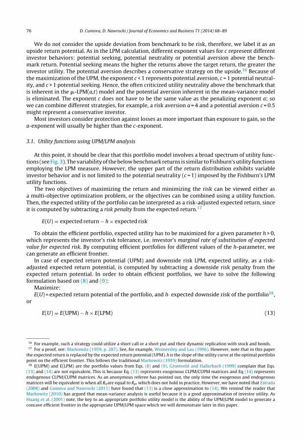
We do not consider the upside deviation from benchmark to be risk, therefore, we label it as anupside return potential. As in the LPM calculation, different exponent values for c represent differentinvestor behaviors: potential seeking, potential neutrality or potential aversion above the bench-mark return. Potential seeking means the higher the returns above the target return, the greater theinvestor utility. The potential aversion describes a conservative strategy on the upside.16 Because ofthe maximization of the UPM, the exponent c < 1 represents potential aversion, c = 1 potential neutral-ity, and c > 1 potential seeking. Hence, the often criticized utility neutrality above the benchmark thatis inherent in the �-LPM(a,t) model and the potential aversion inherent in the mean-variance modelis eliminated. The exponent c does not have to be the same value as the penalizing exponent a; sowe can combine different strategies, for example, a risk aversion a = 4 and a potential aversion c = 0.5might represent a conservative investor.

Most investors consider protection against losses as more important than exposure to gain, so thea-exponent will usually be higher than the c-exponent.

3.1. Utility functions using UPM/LPM analysis

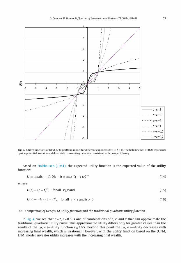
At this point, it should be clear that this portfolio model involves a broad spectrum of utility func-tions (see Fig. 3). The variability of the below benchmark returns is similar to Fishburn’s utility functionsemploying the LPM measure. However, the upper part of the return distribution exhibits variableinvestor behavior and is not limited to the potential neutrality (c = 1) imposed by the Fishburn’s LPMutility functions.

The two objectives of maximizing the return and minimizing the risk can be viewed either asa multi-objective optimization problem, or the objectives can be combined using a utility function.Then, the expected utility of the portfolio can be interpreted as a risk-adjusted expected return, sinceit is computed by subtracting a risk penalty from the expected return.17

E(U) = expected return − h × expected risk

To obtain the efficient portfolio, expected utility has to be maximized for a given parameter h > 0,which represents the investor’s risk tolerance, i.e. investor’s marginal rate of substitution of expectedvalue for expected risk. By computing efficient portfolios for different values of the h-parameter, wecan generate an efficient frontier.

In case of expected return potential (UPM) and downside risk LPM, expected utility, as a risk-adjusted expected return potential, is computed by subtracting a downside risk penalty from theexpected return potential. In order to obtain efficient portfolios, we have to solve the followingformulation based on (8) and (9):

Maximize:E(U) = expected return potential of the portfolio, and h· expected downside risk of the portfolio18,

or

E(U) = E(UPM) − h × E(LPM) (13)

16 For example, such a strategy could utilize a short call or a short put and their dynamic replication with stock and bonds.17 For a proof, see: Markowitz (1959, p. 287). See, for example, Womersley and Lau (1996). However, note that in this paper

the expected return is replaced by the expected return potential (UPM). h is the slope of the utility curve at the optimal portfoliopoint on the efficient frontier. This follows the traditional Markowitz (1959) formulation.

18 E(UPM) and E(LPM) are the portfolio values from Eqs. (8) and (9). Grootveld and Hallerbach (1999) complain that Eqs.(13) and (14) are not equivalent. This is because Eq. (13) represents exogenous CLPM/CUPM matrices and Eq (14) representsendogenous CLPM/CUPM matrices. As an anonymous referee has pointed out, the only time the exogenous and endogenousmatrices will be equivalent is when all Ritare equal to Rpt which does not hold in practice. However, we have noted that Estrada(2008) and Cumova and Nawrocki (2011) have found that (13) is a close approximation to (14). We remind the reader thatMarkowitz (2010) has argued that mean-variance analysis is useful because it is a good approximation of investor utility. AsHuang et al. (2001) note, the key to an appropriate portfolio utility model is the ability of the UPM/LPM model to generate aconcave efficient frontier in the appropriate UPM/LPM space which we will demonstrate later in this paper.

D. Cumova, D. Nawrocki / Journal of Economics and Business 71 (2014) 68– 89 77

Fig. 3. Utility functions of UPM–LPM portfolio model for different exponents (� = 0; h = 1). The bold line (a = c = 0.2) representsupside potential aversion and downside risk-seeking behavior consistent with prospect theory.

Based on Holthausen (1981), the expected utility function is the expected value of the utilityfunction:

U = max[(r − t); 0]c − h × max [(t − r); 0]a (14)

where

U(r) = (r − t)c, for all r≥� and (15)

U(r) = −h × (t − r)a, for all r ≤ � and h > 0 (16)

3.2. Comparison of UPM/LPM utility function and the traditional quadratic utility function

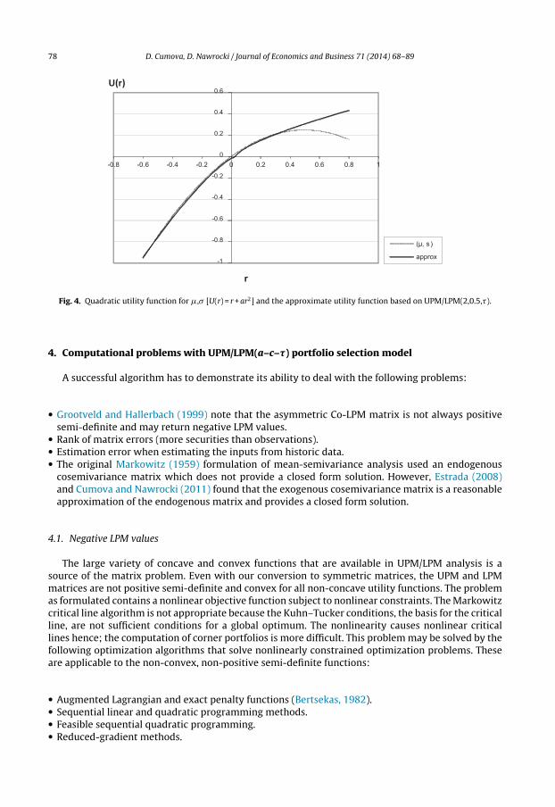
In Fig. 4, we see that a = 2, c = 0.5 is one of combinations of a, c, and � that can approximate thetraditional quadratic utility curve. This approximated utility differs only for greater values than thezenith of the (�, �)—utility function r ≤ 1/2k. Beyond this point the (�, �)—utility decreases withincreasing final wealth, which is irrational. However, with the utility function based on the (UPM,LPM) model, investor utility increases with the increasing final wealth.

78 D. Cumova, D. Nawrocki / Journal of Economics and Business 71 (2014) 68– 89

-1

-0.8

-0.6

-0.4

-0.2

0

0.2

0.4

0.6

-0.8 -0.6 -0.4 -0.2 0 0.2 0.4 0.6 0.8 1

r

(µ, s)

approx

U(r)

Fig. 4. Quadratic utility function for �,� [U(r) = r + ar2] and the approximate utility function based on UPM/LPM(2,0.5,�).

4. Computational problems with UPM/LPM(a–c–�) portfolio selection model

A successful algorithm has to demonstrate its ability to deal with the following problems:

• Grootveld and Hallerbach (1999) note that the asymmetric Co-LPM matrix is not always positivesemi-definite and may return negative LPM values.

• Rank of matrix errors (more securities than observations).• Estimation error when estimating the inputs from historic data.• The original Markowitz (1959) formulation of mean-semivariance analysis used an endogenous

cosemivariance matrix which does not provide a closed form solution. However, Estrada (2008)and Cumova and Nawrocki (2011) found that the exogenous cosemivariance matrix is a reasonableapproximation of the endogenous matrix and provides a closed form solution.

4.1. Negative LPM values

The large variety of concave and convex functions that are available in UPM/LPM analysis is asource of the matrix problem. Even with our conversion to symmetric matrices, the UPM and LPMmatrices are not positive semi-definite and convex for all non-concave utility functions. The problemas formulated contains a nonlinear objective function subject to nonlinear constraints. The Markowitzcritical line algorithm is not appropriate because the Kuhn–Tucker conditions, the basis for the criticalline, are not sufficient conditions for a global optimum. The nonlinearity causes nonlinear criticallines hence; the computation of corner portfolios is more difficult. This problem may be solved by thefollowing optimization algorithms that solve nonlinearly constrained optimization problems. Theseare applicable to the non-convex, non-positive semi-definite functions:

• Augmented Lagrangian and exact penalty functions (Bertsekas, 1982).• Sequential linear and quadratic programming methods.• Feasible sequential quadratic programming.• Reduced-gradient methods.

D. Cumova, D. Nawrocki / Journal of Economics and Business 71 (2014) 68– 89 79

The standard reduced-gradient algorithm19 is implemented in CONOPT, GRG2, LSGRG2 softwareprograms which are available on the NEOS-server for optimization (http://www-neos.mcs.anl.gov).This algorithm works reliably even for large-scale problems. It works by solving a sequence ofsub-problems. Each sub-problem, or major iteration, solves a linearly constrained minimization(maximization) problem. The constraints for this linear sub-problem are the non-linear constraintsconverted to linear using a Taylor expansion series containing first order terms.

A large-scale implementation of the Bertsekas (1982) augmented Lagrangian approach to optimiza-tion can be found in the LANCELOT and MINOS program packages on the NEOS-server. This algorithmalso works reliably for large scale problems.

Negative LPM values noted by Grootveld and Hallerbach (1999) result from three sources: (1) usingan algorithm which requires a matrix that is positive semi-definite, (2) the CLPM Eq. (6) can returna negative value whenever a < 1, and (3) when there is a rank of matrix error (more securities thanobservations).

Note that Eq. (6) applies for a > 1. However, whenever 0 < a < 1, (6) can result in anomalies withnegative portfolio risk. Therefore, we propose the following computational equation which is operativefor all values of a:20

E(CLPMij) = 1/K

K∑t=1

Max[0, (� − rit)]a/2 · |� − rjt |a/2 · sign(� − rjt) (17)

4.2. Rank of matrix error

The rank of matrix error is the source of many anomalies associated with portfolio selection algo-rithms. Essentially, it occurs whenever there are more securities in the analysis than the number ofobservations used to estimate the inputs. Markowitz (1959) notes that this is a “degrees of freedom”problem similar to multiple regression. In addition, Klein and Bawa (1977) identify it as a major sourceof estimation error. Very simply, algorithms that are sensitive to the rank of matrix error will returnnon-optimal solutions or will not reach an optimum solution (singular matrix error). Markowitz (1987)derives the conditions necessary for an algorithm to be robust relative to rank of matrix error and goeson to show that the critical line algorithm is not sensitive to the rank of matrix error. While the criticalline algorithm may not be appropriate for this optimization, the algorithms used in this study havebeen shown to have a low degree of sensitivity to rank of matrix error, however, it is best to minimizethe error by maintaining sufficient positive degrees of freedom. In addition, the rank of matrix errorhas not been shown to be a problem until more than 50 securities are used in the analysis.21 Sincemost portfolio optimization applications do not use more than 50 securities, this problem is minimalbut should be noted whenever large security universes are used.

4.3. Estimation risk

Even with the improved algorithms, estimation error remains a problem. Grootveld and Hallerbach(1999) provide evidence that the estimation error for the optimization inputs is more prevalent forLPM analysis because it uses only part of the distribution. Kaplan and Siegel (1994a, 1994b) also notethe small sample problem when using LPM measures.

There have not been very many studies on estimating LPM from data. Nawrocki (1992) found thatwhen the rank of matrix error is minimized, the LPM measure for different degrees stabilizes around 48monthly observations. The variance and beta needed sample sizes larger than 72 months to stabilize.Josephy and Aczel (1993) derived a sample estimator for the semivariance and showed that it was

19 Lasdon and Warren (1978, pp. 335–362).20 Because the UPM is a mirror image of the LPM, this correction also applies to the CUPM computation whenever 0 < c < 1.

Eqs. (6) and (19) are mathematically equivalent when a ≥ 1. However, (17) will not return negative values whenever a < 1.21 Cumova and Nawrocki (2011).

80 D. Cumova, D. Nawrocki / Journal of Economics and Business 71 (2014) 68– 89

asymptotically unbiased and strongly consistent, thus possessing qualities of a ‘good’ estimator. Theyrecommend the use of the semivariance whenever the underlying distribution is skewed. Bond andSatchell (2002) found that the variance is a more volatile risk measure than semivariance when returndistributions are asymmetric. When return distributions are symmetric, then the variance is the moreefficient measure. As asymmetric distributions are cited as the most common reason for utilizing LPMrisk measures, these results would support the use of LPM measures.

In actual investment practice and in academic empirical studies, bootstrapping techniques suchas Efron and Tibshirani (1993) may be employed. Sortino and Forsey (1996) demonstrate the useof bootstrapping with the LPM measure. Bootstrapping simulation is used in this study to minimizeestimation error. Other methods include James-Stein estimators proposed by Jobson and Korkie (1980)and Michaud’s (1989) re-sampled frontier technique. Elton and Gruber (1973) and Elton, Gruber, andUrich (1978) demonstrate that overall mean models implemented in simple heuristics reduce thedegree of estimation risk. In real-world practice, a UPM/LPM heuristic based on the overall meanmodel of Elton, Gruber, and Padberg (1976) may prove to be the most useful application of UPM/LPManalysis.

4.4. Exogenous and endogenous Co-LPM and Co-UPM matrices

Estrada (2008) provides a good description of exogenous and endogenous cosemivariance (Co-LPM)matrices that will also affect Co-UPM matrices. Essentially, the cosemivariance matrix as formulatedby Markowitz (1959) cannot be computed until we know the portfolio returns which we do not knowuntil we know the portfolio allocations. Therefore, the mean-semivariance problem is not a closed-form solution because the cosemivariance matrix is endogenous. Estrada (2008) finds that a computedexogenous cosemivariance matrix can closely approximate the endogenous matrix. Thus, any closedform UPM/LPM optimization algorithm does rest on this exogenous matrix approximation. On theother hand, the endogenous matrix is not part of our information set when we start the analysis.Currently, the only algorithms we have to estimate UPM/LPM efficient portfolios are mean-variance(covariance) and mean-LPM (Co-LPM) algorithms. Therefore, the empirical test in this paper comparesoptimal UPM/LPM portfolios to optimal mean-variance and mean-LPM portfolios to test the usefulnessof the UPM/LPM exogenous matrix algorithm. In all cases the appropriate covariance, CLPM, and CUPMmatrix is used in a closed form optimization.

5. Four UPM–LPM utility cases

The next section of the paper presents four utility cases with different concave and convex functionsto illustrate the use of the UPM/LPM model.

5.1. Concave efficient frontiers

Hogan and Warren (1972, 1974), Bawa (1975), Bawa and Lindenberg (1977), Harlow and Rao (1989)provide proofs that �-LPM efficient frontier is concave. Pedersen and Satchell (2002) provide theproof for �-semistandard deviation frontiers. Huang et al. (2001) provide empirical support for theexogenous matrix model generating concave frontiers. As an extension of the Hogan and Warren(1972) corollary, we state that the UPM/LPM efficient frontier is concave when the UPM of efficientportfolios in the UPM/LPM space is concave as a function of the LPM. We demonstrate this concaveresult in the next section through an empirical example. The issue is whether the UPM/LPM algorithmscan generate a concave efficient frontier in the UPM/LPM(a,c,�) space as per Hogan and Warren (1972).The only other algorithms that we have to test the UPM/LPM model against are the mean-variance(�-�) and mean-semivariance (�-LPM degree 2) algorithms. In order to compare different algorithmsin the appropriate UPM/LPM space, the efficient frontiers and appropriate statistics are computedusing portfolio returns (equation 1) generated by the algorithms. Therefore, there are no exogenous-endogenous matrix issues with these results.

D. Cumova, D. Nawrocki / Journal of Economics and Business 71 (2014) 68– 89 81

Table 1Generated summary statistics for 12 assets used in the four utility cases: stocks (S), covered calls (CC), and protective puts (PP).

Input parameters for the various securities (S) stocks, (CC) covered calls, and (PP) protective puts in the optimization

Asset Mean Std.Dev SemiDev Skewness

S1 0.185 0.382 0.187 0.166S2 0.079 0.230 0.133 −0.060S3 0.215 0.462 0.210 0.380S4 0.175 0.351 0.160 0.413CC1 0.179 0.195 0.132 −2.937CC2 0.095 0.115 0.081 −2.916CC3 0.179 0.217 0.139 −2.050CC4 0.146 0.160 0.111 −3.074PP1 0.052 0.241 0.128 1.372PP2 0.022 0.147 0.096 0.913PP3 0.065 0.296 0.135 1.294PP4 0.059 0.239 0.109 1.518

Correlation matrix for the 12 assets

S1 S2 S3 S4 CC1 CC2 CC3 CC4 PP1 PP2 PP3 PP4

S1 1.00 0.57 0.73 0.46 0.72* 0.50 0.52 0.32 0.93* 0.49 0.69 0.42S2 0.57 1.00 0.59 0.28 0.51 0.78* 0.50 0.26 0.48 0.93* 0.52 0.22S3 0.73 0.59 1.00 0.51 0.49 0.51 0.71* 0.35 0.70 0.51 0.95* 0.48S4 0.46 0.28 0.51 1.00 0.41 0.27 0.31 0.68* 0.39 0.22 0.51 0.94*CC1 0.72 0.51 0.49 0.41 1.00 0.65 0.61 0.55 0.42* 0.32 0.34 0.26CC2 0.50 0.78 0.51 0.27 0.65 1.00 0.56 0.27 0.32 0.49* 0.39 0.21CC3 0.52 0.50 0.71 0.31 0.61 0.56 1.00 0.31 0.37 0.36 0.45* 0.24CC4 0.32 0.26 0.35 0.68 0.55 0.27 0.31 1.00 0.13 0.20 0.30 0.38*PP1 0.93 0.48 0.70 0.39 0.42 0.32 0.37 0.13 1.00 0.48 0.72 0.42PP2 0.49 0.93 0.51 0.22 0.32 0.49 0.36 0.20 0.48 1.00 0.49 0.19PP3 0.69 0.52 0.95 0.51 0.34 0.39 0.45 0.30 0.72 0.49 1.00 0.50PP4 0.42 0.22 0.48 0.94 0.26 0.21 0.24 0.38 0.42 0.19 0.50 1.00

5.2. Summary of assets used in four UPM–LPM utility cases

To help present these cases with significantly non-normal security distributions, 12 assets wereutilized. The first four assets are stocks. The second four assets are the result of writing covered calloptions on the first four stocks. The last four assets represent the purchase of covered puts on the firstfour stocks.

A Monte Carlo simulation is run to estimate 3000 security returns for the four stocks using a normaldistribution random number generator and the parameters and correlations are presented in Table 1.The returns for the covered call and protective put positions are computed using the methodology pro-posed by Bookstaber and Clarke (1983, 1984).22 Four random numbers (Wiener process) are generatedfor each stock for one iteration and then the Cholesky matrix (factorization) is used to obtain corre-lated returns. With every stock return, the call strategy returns and put strategy returns are computedapplying Black–Scholes formula. From the obtained return series, the additional correlations betweenthe put and call return series are computed.

As can be seen, the assets present a wide spectrum of high and low returns, high and low standarddeviations, and positive and negative skewness in order to demonstrate the properties of the UPM/LPMmodel. The same optimization algorithm (the Augmented Lagrangian by Bertsekas, 1982) was used tocompute mean-variance, mean-LPM, and UPM/LPM efficient frontiers.23

22 This allows the Monte Carlo simulation to start with a Gaussian distribution and then positive and negative skewnessdistributions are added with the put and call positions, respectively. Huang et al. (2001) and Coval and Shumway (2001) alsoprovide methods for computing portfolio returns for optioned portfolios.

23 All non-linear formulations use the basic model described by Eqs. (8)–(10), (13) and (17).

82 D. Cumova, D. Nawrocki / Journal of Economics and Business 71 (2014) 68– 89

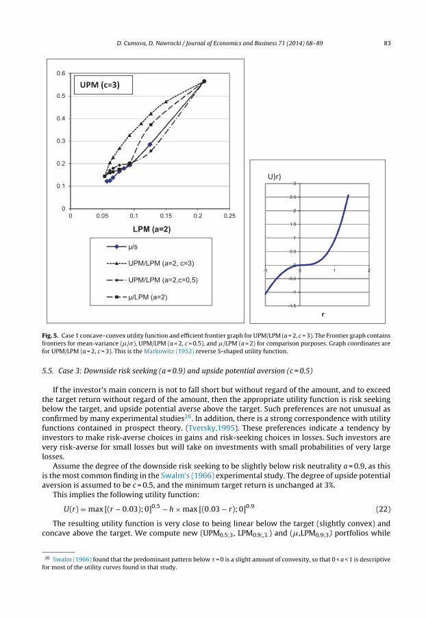
5.3. Case 1: Downside risk aversion (a = 2) and upside potential seeking (c = 3)

This is probably a very common case where investors wish to reduce downside risk while at thesame time preserving as much of the upside returns as economically feasible. This means that theinvestor is risk averse below the target return and upside potential seeking above the target. Theutility function expressing such preferences is the Markowitz (1952) reverse S-shaped function, whichmeans that it is concave below the target return and convex above the target.

In the utility function, where return deviations from some reference point are evaluated by someexponent, risk aversion is represented by an exponent a > 1, and upside seeking is represented by c > 1.In this example, we assume that the degree of risk aversion is identified a = 2, and degree of upsidepotential seeking is c = 3. The minimum target return is set equal to the risk free return of 3%. Theutility function U(r) is defined as:

U(r) = (r − 0.03)3, for all r≥0.03, and (18)

U(r) = −h × (0.03 − r)2, for all r < 0.03 or (19)

U(r) = max [(r − 0.03); 0]3 − h × max [(0.03 − r); 0]2 (20)

The efficient frontier of portfolios with maximal expected utility we obtain by varying the slope –h-parameter – by the maximization of the EU(r) using input data from Table 1.24 The efficient frontiersare computed using the (UPM3,3, LPM2,3), (�,LPM2,3), and (�, �) portfolio models.

Using the (UPM3,3, LPM2,3) coordinate system (Fig. 5), we see that the UPM/LPM(2,3,3) frontierrepresents a successful result where the UPM is a concave function of the LPM. Note that the otherfrontiers are not concave in the UPM/LPM(2,3,3)space.

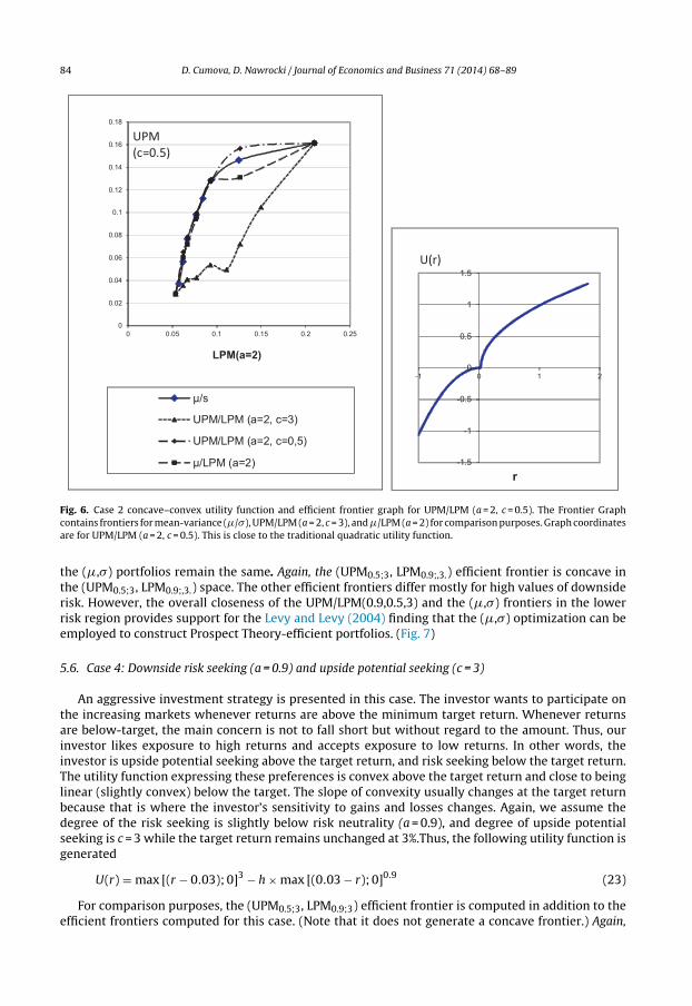
5.4. Case 2: Downside risk aversion (a = 2) and upside potential aversion (c = 0.5)

As investors differ in their preferences, it is possible that many of them are downside risk averseand upside potential averse. Such a preference corresponds with a conservative investment strategywhere the investor is everywhere risk averse. This strategy would try to concentrate returns towardsome target return (t). The implied utility function is concave as assumed in the classical theory ofexpected utility. In the following example, we assume that the degree of upside potential aversion isc = 0.5 and the degree of downside risk aversion is a = 225. The minimum target return (t) is set equalto risk free return of 3%.

Assume the following utility function:

U(r) = max [(r − 0.03); 0]0.5 − h × max [(0.03 − r); 0]2 (21)

The general UPM and LPM measures we define according to the assumed utility function as UPMc;t

and LPMa;t or UPM00.5;3, and LPM2;3. The first part of the equation of the expected utility functioncorresponds with the applied UPM and the second part with the LPM measure.

We obtain the efficient frontier of portfolios with maximal expected utility by varying the slope –h-parameter – in the EU(r) optimization formulation. Again, the UPM/LPM(2,0.5,3) frontier is concave inthe UPM/LPM(2,0.5,3) space. The (UPM0.5;3, LPM2;3.), (�,�), and (�,LPM2;3) portfolios provide roughlythe same efficient frontiers except in the higher risk area where the �,LPM(2,3) frontier is not con-cave. This result makes sense as the utility function for UPM/LPM(2,0.5,3) approximates the quadraticfunction inherent in (�,�) formulation. An alternative strategy, (UPM3;3, LPM2,3), where the investorhas strong emphasis on seeking upside potential generates portfolios with significantly higher riskand a non-concave efficient frontier. (Fig. 6)

24 The efficient frontiers were generated using the Augmented Lagrangian algorithm developed by Bertsekas (1982). TheLANCELOT program package on the NEOS server (http://www-neos.mcs.anl.gov) provides access to this algorithm for largescale optimizations.

25 See the method for estimation of degree of risk aversion and potential seeking in the appendix of this paper.

D. Cumova, D. Nawrocki / Journal of Economics and Business 71 (2014) 68– 89 83

0

0.1

0.2

0.3

0.4

0.5

0.6

0 0.05 0.1 0.15 0.2 0.25

LPM (a=2)

µ/s

UPM/LPM (a=2, c=3)

UPM/LPM (a=2, c=0 ,5)

µ/LPM (a=2)-1.5

-1

-0.5

0

0.5

1

1.5

2

2.5

3

-1 0 1 2

r

U)r)

UPM (c=3)

Fig. 5. Case 1 concave–convex utility function and efficient frontier graph for UPM/LPM (a = 2, c = 3). The Frontier graph containsfrontiers for mean-variance (�/�), UPM/LPM (a = 2, c = 0.5), and �/LPM (a = 2) for comparison purposes. Graph coordinates arefor UPM/LPM (a = 2, c = 3). This is the Markowitz (1952) reverse S-shaped utility function.

5.5. Case 3: Downside risk seeking (a = 0.9) and upside potential aversion (c = 0.5)

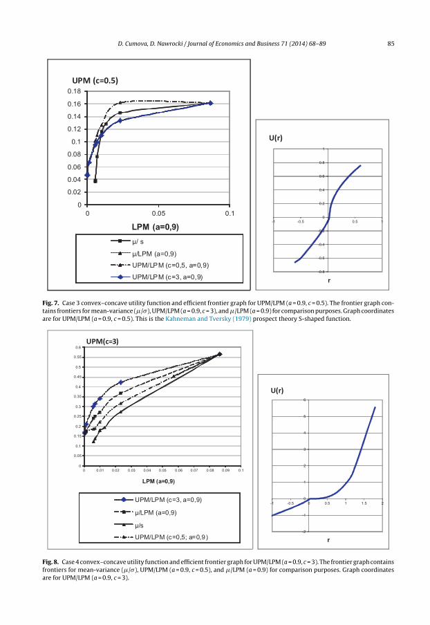
If the investor’s main concern is not to fall short but without regard of the amount, and to exceedthe target return without regard of the amount, then the appropriate utility function is risk seekingbelow the target, and upside potential averse above the target. Such preferences are not unusual asconfirmed by many experimental studies26. In addition, there is a strong correspondence with utilityfunctions contained in prospect theory. (Tversky,1995). These preferences indicate a tendency byinvestors to make risk-averse choices in gains and risk-seeking choices in losses. Such investors arevery risk-averse for small losses but will take on investments with small probabilities of very largelosses.

Assume the degree of the downside risk seeking to be slightly below risk neutrality a = 0.9, as thisis the most common finding in the Swalm’s (1966) experimental study. The degree of upside potentialaversion is assumed to be c = 0.5, and the minimum target return is unchanged at 3%.

This implies the following utility function:

U(r) = max [(r − 0.03); 0]0.5 − h × max [(0.03 − r); 0]0.9 (22)

The resulting utility function is very close to being linear below the target (slightly convex) andconcave above the target. We compute new (UPM0.5;3, LPM0.9;,3.) and (�,LPM0.9;3) portfolios while

26 Swalm (1966) found that the predominant pattern below � = 0 is a slight amount of convexity, so that 0 < a < 1 is descriptivefor most of the utility curves found in that study.

84 D. Cumova, D. Nawrocki / Journal of Economics and Business 71 (2014) 68– 89

0

0.02

0.04

0.06

0.08

0.1

0.12

0.14

0.16

0.18

0 0.05 0.1 0.15 0.2 0.25

LPM(a=2)

µ/s

UPM/LPM (a= 2, c =3)

UPM/LPM (a= 2, c =0,5 )

µ/LPM (a =2)

UPM(c=0.5)

-1.5

-1

-0.5

0

0.5

1

1.5

-1 0 1 2

r

U(r)

Fig. 6. Case 2 concave–convex utility function and efficient frontier graph for UPM/LPM (a = 2, c = 0.5). The Frontier Graphcontains frontiers for mean-variance (�/�), UPM/LPM (a = 2, c = 3), and �/LPM (a = 2) for comparison purposes. Graph coordinatesare for UPM/LPM (a = 2, c = 0.5). This is close to the traditional quadratic utility function.

the (�,�) portfolios remain the same. Again, the (UPM0.5;3, LPM0.9;,3.) efficient frontier is concave inthe (UPM0.5;3, LPM0.9;,3.) space. The other efficient frontiers differ mostly for high values of downsiderisk. However, the overall closeness of the UPM/LPM(0.9,0.5,3) and the (�,�) frontiers in the lowerrisk region provides support for the Levy and Levy (2004) finding that the (�,�) optimization can beemployed to construct Prospect Theory-efficient portfolios. (Fig. 7)

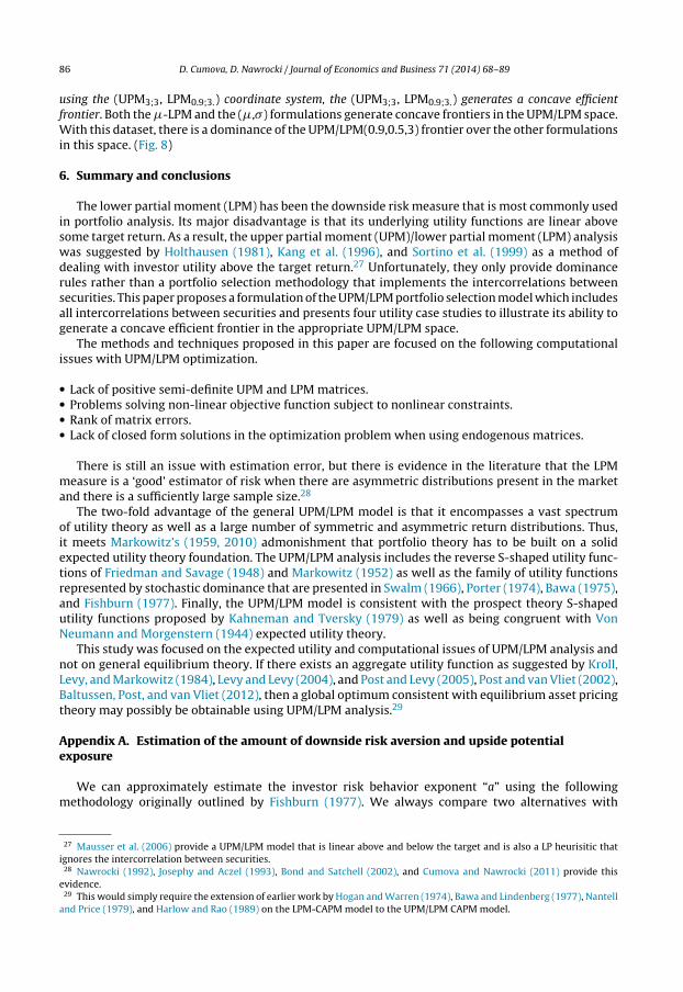
5.6. Case 4: Downside risk seeking (a = 0.9) and upside potential seeking (c = 3)

An aggressive investment strategy is presented in this case. The investor wants to participate onthe increasing markets whenever returns are above the minimum target return. Whenever returnsare below-target, the main concern is not to fall short but without regard to the amount. Thus, ourinvestor likes exposure to high returns and accepts exposure to low returns. In other words, theinvestor is upside potential seeking above the target return, and risk seeking below the target return.The utility function expressing these preferences is convex above the target return and close to beinglinear (slightly convex) below the target. The slope of convexity usually changes at the target returnbecause that is where the investor’s sensitivity to gains and losses changes. Again, we assume thedegree of the risk seeking is slightly below risk neutrality (a = 0.9), and degree of upside potentialseeking is c = 3 while the target return remains unchanged at 3%.Thus, the following utility function isgenerated

U(r) = max [(r − 0.03); 0]3 − h × max [(0.03 − r); 0]0.9 (23)

For comparison purposes, the (UPM0.5;3, LPM0.9;3) efficient frontier is computed in addition to theefficient frontiers computed for this case. (Note that it does not generate a concave frontier.) Again,

D. Cumova, D. Nawrocki / Journal of Economics and Business 71 (2014) 68– 89 85

0

0.02

0.04

0.06

0.08

0.1

0.12

0.14

0.16

0.18

0 0.05 0.1

LPM (a=0,9 )

µ/ s

µ/LPM (a=0,9)

UPM/LPM (c=0,5, a=0,9)

UPM/LPM (c=3, a=0,9)

UPM (c=0.5)

-0.8

-0.6

-0.4

-0.2

0

0.2

0.4

0.6

0.8

1

-1 -0.5 0 0.5 1

r

U(r)

Fig. 7. Case 3 convex–concave utility function and efficient frontier graph for UPM/LPM (a = 0.9, c = 0.5). The frontier graph con-tains frontiers for mean-variance (�/�), UPM/LPM (a = 0.9, c = 3), and �/LPM (a = 0.9) for comparison purposes. Graph coordinatesare for UPM/LPM (a = 0.9, c = 0.5). This is the Kahneman and Tversky (1979) prospect theory S-shaped function.

0

0.05

0.1

0.15

0.2

0.25

0.3

0.35

0.4

0.45

0.5

0.55

0.6

0 0.01 0.02 0.0 3 0.04 0.05 0.06 0.07 0.08 0.09 0.1

LPM (a=0,9 )

UPM /LPM (c=3, a=0, 9)

µ/LPM (a=0,9)

µ/s

UPM/LPM (c=0,5; a=0,9)

UPM (c=3 )

-2

-1

0

1

2

3

4

5

6

-1 -0. 5 0 0. 5 1 1.5 2

r

U(r)

Fig. 8. Case 4 convex–concave utility function and efficient frontier graph for UPM/LPM (a = 0.9, c = 3). The frontier graph containsfrontiers for mean-variance (�/�), UPM/LPM (a = 0.9, c = 0.5), and �/LPM (a = 0.9) for comparison purposes. Graph coordinatesare for UPM/LPM (a = 0.9, c = 3).

86 D. Cumova, D. Nawrocki / Journal of Economics and Business 71 (2014) 68– 89

using the (UPM3;3, LPM0.9;3.) coordinate system, the (UPM3;3, LPM0.9;3.) generates a concave efficientfrontier. Both the �-LPM and the (�,�) formulations generate concave frontiers in the UPM/LPM space.With this dataset, there is a dominance of the UPM/LPM(0.9,0.5,3) frontier over the other formulationsin this space. (Fig. 8)

6. Summary and conclusions

The lower partial moment (LPM) has been the downside risk measure that is most commonly usedin portfolio analysis. Its major disadvantage is that its underlying utility functions are linear abovesome target return. As a result, the upper partial moment (UPM)/lower partial moment (LPM) analysiswas suggested by Holthausen (1981), Kang et al. (1996), and Sortino et al. (1999) as a method ofdealing with investor utility above the target return.27 Unfortunately, they only provide dominancerules rather than a portfolio selection methodology that implements the intercorrelations betweensecurities. This paper proposes a formulation of the UPM/LPM portfolio selection model which includesall intercorrelations between securities and presents four utility case studies to illustrate its ability togenerate a concave efficient frontier in the appropriate UPM/LPM space.

The methods and techniques proposed in this paper are focused on the following computationalissues with UPM/LPM optimization.

• Lack of positive semi-definite UPM and LPM matrices.• Problems solving non-linear objective function subject to nonlinear constraints.• Rank of matrix errors.• Lack of closed form solutions in the optimization problem when using endogenous matrices.

There is still an issue with estimation error, but there is evidence in the literature that the LPMmeasure is a ‘good’ estimator of risk when there are asymmetric distributions present in the marketand there is a sufficiently large sample size.28

The two-fold advantage of the general UPM/LPM model is that it encompasses a vast spectrumof utility theory as well as a large number of symmetric and asymmetric return distributions. Thus,it meets Markowitz’s (1959, 2010) admonishment that portfolio theory has to be built on a solidexpected utility theory foundation. The UPM/LPM analysis includes the reverse S-shaped utility func-tions of Friedman and Savage (1948) and Markowitz (1952) as well as the family of utility functionsrepresented by stochastic dominance that are presented in Swalm (1966), Porter (1974), Bawa (1975),and Fishburn (1977). Finally, the UPM/LPM model is consistent with the prospect theory S-shapedutility functions proposed by Kahneman and Tversky (1979) as well as being congruent with VonNeumann and Morgenstern (1944) expected utility theory.

This study was focused on the expected utility and computational issues of UPM/LPM analysis andnot on general equilibrium theory. If there exists an aggregate utility function as suggested by Kroll,Levy, and Markowitz (1984), Levy and Levy (2004), and Post and Levy (2005), Post and van Vliet (2002),Baltussen, Post, and van Vliet (2012), then a global optimum consistent with equilibrium asset pricingtheory may possibly be obtainable using UPM/LPM analysis.29

Appendix A. Estimation of the amount of downside risk aversion and upside potentialexposure

We can approximately estimate the investor risk behavior exponent “a” using the followingmethodology originally outlined by Fishburn (1977). We always compare two alternatives with

27 Mausser et al. (2006) provide a UPM/LPM model that is linear above and below the target and is also a LP heurisitic thatignores the intercorrelation between securities.

28 Nawrocki (1992), Josephy and Aczel (1993), Bond and Satchell (2002), and Cumova and Nawrocki (2011) provide thisevidence.

29 This would simply require the extension of earlier work by Hogan and Warren (1974), Bawa and Lindenberg (1977), Nantelland Price (1979), and Harlow and Rao (1989) on the LPM-CAPM model to the UPM/LPM CAPM model.

D. Cumova, D. Nawrocki / Journal of Economics and Business 71 (2014) 68– 89 87

the same UPM, but with different LPM values. In the first example, we can lose A—amount withp—probability. In the second example, we can lose B—amount with the same probability p, but fortwo states. Using the exponent a = 1, i.e. risk neutrality, we would be indifferent between these twoalternatives for the B-amount equal to A/2.

p · A1 = p · B1 + p · B1

p · A1 = p ·(

A

2

)1

+ p ·(

A

2

)1 (24)

If we prefer the second alternative, we would have a higher grade of risk aversion because thissecond alternative has a lower total loss for all cases of higher risk aversion, or a > 1. To compute theamount of risk aversion, we will have to compare the same two alternatives with a higher degree ofrisk aversion, for example a = 2.

p · A2 = p · B2 + p · B2

p · A2 = p ·(

A2√2

)2

+ p ·(

A2√2

)2 (25)

If we have the degree of risk aversion a = 2, we would be indifferent between the loss of A—amountwith p—probability and the loss of A/

√2 amount with the same probability p. If we prefer the second

alternative, we have a higher degree of risk aversion than a = 2. So, we have to repeat the comparisonof these two alternatives for higher and higher degrees of a. For example, for the case a = 3, we areindifferent between the alternatives, where the loss of B in the second alternative is equal to A/ 3√2. Ifwe prefer the second alternative, then we have even a higher degree of risk aversion, and we have torepeat the comparison until we find indifferent alternatives.

In case of a risk seeking investor, we would prefer by the first alternative when a = 1. From there, wehave to reduce the degree of risk seeking behavior (a < 1) until we reach indifference. For the degreeof return exposure in the upper part of distribution “c”, we proceed the same way, however, potentialseeking behavior is c > 1 and the conservative strategy on the upside is 0 < c < 1.

Note that Fishburn (1977), Laughhunn, Payne, and Crum (1980), and Holthausen (1981) all concludethat the a coefficient is sensitive to the total wealth of the investor, i.e. how much is at risk relative tototal wealth affects the investor’s a coefficient.

References

Ang, J. S. (1975). A note on the E, SL portfolio selection model. Journal of Financial and Quantitative Analysis, 10(5), 849–857.Baltussen, G., Post, T., & van Vliet, P. (2006). Violations of cumulative prospect theory in mixed gambles with moderate proba-

bilities. Management Science, 52(8), 1288–1290.Baltussen, G., Post, G. T., & Vliet, P. V. (2012). Downside risk aversion, fixed-income exposure, and the value premium puzzle.

Journal of Banking & Finance,Barnes, J. D., & Reinmuth, J. E. (1976). Comparing imputed and actual utility functions in a competitive bidding setting. Decision

Sciences, 7(4), 801–812.Bawa, V. S. (1975). Optimal rules for ordering uncertain prospects. Journal of Financial Economics, 2(1), 95–121.Bawa, V. S., & Lindenberg, E. B. (1977). Capital market equilibrium in a mean-lower partial moment framework. Journal of

Financial Economics, 5(2), 189–200.Bawa, V. S., Brown, S., & Klein, R. (1981). Asymmetric response asset pricing models: Testable alternatives to mean–variance.

Mimeo.Bertsekas, D. P. (1982). Constrained optimization and Lagrangian multiplier methods. New York: Athena Scientific (paperback

edition, 1996).Bond, S. A., & Satchell, S. E. (2002). Statistical properties of the sample semi-variance. Applied Mathematical Finance, 9, 219–239.Bookstaber, R., & Clarke, R. (1983). An algorithm to calculate the return distribution of portfolios with option positions. Man-

agement Science, 29(4), 419–429.Bookstaber, R., & Clarke, R. (1984). Option portfolio strategies: Measurement and evaluation. Journal of Business, 57(4), 469–492.Coval, J. D., & Shumway, T. (2001). Expected option returns. Journal of Finance, 56(3), 983–1009.Cumova, D., & Nawrocki, D. (2011). A symmetric LPM model for mean-semivariance analysis. Journal of Economics and Business,

63(3), 217–236.Efron, B., & Tibshirani, R. (1993). An introduction to the boot strap. London: Chapman and Hall.Elton, E. J., & Gruber, M. J. (1973). Estimating the dependence structure of share prices—Implications for portfolio selection.

Journal of Finance, 28(5), 1203–1232.

88 D. Cumova, D. Nawrocki / Journal of Economics and Business 71 (2014) 68– 89

Elton, E. J., Gruber, M. J., & Padberg, M. W. (1976). Simple criteria for optimal portfolio selection. Journal of Finance, 31(5),1341–1357.

Elton, Edwin J., Gruber, Martin J., & Urich, Thomas J. (1978). Are betas best? Journal of Finance, 33(5), 1375–1384.Estrada, Javier. (2008). Mean-semivariance optimization: A heuristic approach. Journal of Applied Finance, 18(1), 57–72.Fishburn, P. C. (1977). Mean-risk analysis with risk associated with below-target returns. American Economic Review, 67(2),

116–126.Fishburn, P. C., & Kochenberger, G. A. (1979). Two-piece Von Neumann–Morgenstern utility functions. Decision Sciences, 10,

503–518.Francis, J. C., & Archer, S. H. (1979). Portfolio analysis (2nd ed.). Englewood Cliffs, NJ: Prentice Hall, Inc.Friedman, M., & Savage, L. J. (1948). The utility analysis of choices involving risk. Journal of Political Economy, 56, 279–304.Frowein, W. (2000). On the consistency of mean-lower partial moment analysis and expected utility maximisation working paper.

Ludwig–Maximilian-University of Munich, Institute of Capital Market and Research.Grayson, C. J. (1960). Decisions under uncertainty: Drilling decisions by oil and gas operators. Cambridge, MA: Graduate School of

Business, Harvard University.Green, P. E. (1963). Risk attitudes and chemical investment decisions. Chemical Engineering Progress, 59, 35–40.Grootveld, H., & Hallerbach, W. (1999). Variance vs. downside risk: Is there really that much difference. European Journal of

Operational Research, 114, 304–319.Halter, A. N., & Dean, G. W. (1971). Decisions under uncertainty. Cincinnati, OH: Cincinnati.Harlow, W. V., & Rao, R. K. S. (1989). Asset pricing in a generalized mean-lower partial moment framework: Theory and evidence.

Journal of Financial and Quantitative Analysis, 24(3), 285–312.Hogan, W. W., & Warren, J. M. (1972). Computation of the efficient boundary in the E–S portfolio selection model. Journal of

Financial and Quantitative Analysis, 7(4), 1881–1896.Hogan, W. W., & Warren, J. M. (1974). Toward the development of an equilibrium capital-market model based on semivariance.

Journal of Financial and Quantitative Analysis, 9(1), 1–11.Holthausen, D. M. (1981). A risk–return model with risk and return measured as deviations from a target return. American

Economic Review, 71(1), 182–188.Huang, T., Srivastava, V., & Raatz, S. (2001). Portfolio optimisation with options in the foreign exchange market. Derivatives Use,

Trading, and Regulation, 7(1), 55–72.Jarrow, R., & Zhao, F. (2006). Downside risk aversion and portfolio management. Management Science, 52(2, April), 558–566.Jobson, J. D., & Korkie, B. (1980). Estimation for Markowitz efficient portfolios. Journal of the American Statistical Association,

75(371), 544–554.Josephy, N. H., & Aczel, A. D. (1993). A statistically optimal estimator of semivariance. European Journal of Operational Research,

67, 267–271.Kahneman, D., & Tversky, A. (1979). Prospect theory: An analysis of decision under risk. Econometrica, 47(2), 263–292.Kang, T., Brorsen, B. W., & Adam, B. D. (1996). A new efficiency criterion: The mean-separated target deviations risk model.

Journal of Economics and Business, 48, 47–66.Kaplan, P. D., & Siegel, L. B. (1994a). Portfolio theory is alive and well. Journal of Investing, 3(3), 18–23.Kaplan, P. D., & Siegel, L. B. (1994b). Portfolio theory is still alive and well. Journal of Investing, 3(3), 45–46.Klein, R. W., & Bawa, V. S. (1977). The effect of limited information and estimation risk on optimal portfolio diversification.

Journal of Financial Economics, 5(1), 89–111.Konno, H., Tanaka, K., & Yamamoto, R. (2011). Construction of a portfolio with shorter downside tail and longer upside tale.

Computational Optimization and Applications, 48(2), 199–212.Kroll, Y., Levy, H., & Markowitz, H. M. (1984). Mean-variance versus direct utility maximization. Journal of Finance, 39(1), 47–62.Lasdon, L., & Warren, A. D. (1978). Generalized reduced gradient software for linearly and nonlinearly constrained problems.

In J. H. Greenberg (Ed.), Design and implementation of optimization software (pp. 335–362). The Netherlands: Sijthoff andNoordhoff.

Laughhunn, D. J., Payne, J. W., & Crum, R. (1980). Managerial risk preferences for below-target returns. Management Science,25(12), 921–940. December.

Leland, H. E. (1999). Beyond mean-variance: Performance measurement in a nonsymmetrical World. Financial Analyst Journal,55 (Jan/Feb), 27–36.

Levy, H. (1998). Stochastic dominance. Norwell, MA: Kluwer Academic Publishers.Levy, M., & Levy, H. (2002). Prospect theory: Much ado about nothing. Management Science, 48(10), 1334–1349.Levy, H., & Levy, M. (2004). Prospect theory and mean-variance analysis. The Review of Financial Studies, 17(4), 1015–1041.

Winter.Markowitz, H. (1952). The utility of wealth. Journal of Political Economy, 60(2), 151–158.Markowitz, H. (1959). Portfolio selection (1st ed.). New York: John Wiley and Sons.Markowitz, H. (1987). Mean-variance analysis in portfolio choice and capital markets (1st ed.). New York: Basil Blackwell.Markowitz, H., Todd, P., Xu, G., & Yamane, Y. (1993). Computation of mean-semivariance efficient sets by the critical line

algorithm. Annals of Operations Research, 45, 307–317.Markowitz, H. (2010). Porfolio theory: As I still see it. Annual Review of Financial Economics, 2, 1–41.Mausser, H., Saunders, D., & Seco, L. (2006). Optimising omega. Risk, 19(11), 88–92.Merriken, H. E. (1994). Analytical approaches to limit downside risk: Semivariance and the need for liquidity. Journal of Investing,

3(3), 65–72.Michaud, R. O. (1989). The Markowitz optimization Enigma: Is ‘Optimized’ optimal? Financial Analyst Journal, 45(1),

31–42.Musiol, G., & Muhlig, H. (2003). Taschenbuch der Mathematick. http://www.tu-chemnitz.de/service/lirech/DTbron5.1/daten/kap

4/node62.htm (accessed 10.10.2003)Nantell, T. J., & Price, B. (1979). An analytical comparison of variance and semivariance capital market theories. Journal of Financial

and Quantitative Analysis, 14(2), 221–242.Nawrocki, D. N. (1991). Optimal algorithms and lower partial moments: Ex post results. Applied Economics, 23, 465–470.

D. Cumova, D. Nawrocki / Journal of Economics and Business 71 (2014) 68– 89 89

Nawrocki, D. N. (1992). The characteristics of portfolios selected by n-degree lower partial moment. International Review ofFinancial Analysis, 1(3), 195–210.

Ogryczak, W., & Ruszczynski, A. (2001). On consistency of stochastic dominance and mean-semideviation models. MathematicalProgramming, Series B, 89, 217–232.

Pedersen, C. S. (2001). Derivatives and downside risk. Derivatives Use, Trading and Regulation, 7(1).Pedersen, C. S., & Satchell, S. E. (2000). Small sample analysis of performance measures in the asymmetric response model.

Journal of Financial and Quantitative Analysis, 35(3), 425–450.Pedersen, C. S., & Satchell, S. E. (2002). On the foundation of performance measures under asymmetric returns. Quantitative

Finance, 2, 217–223.Porter, R. B. (1974). Semivariance and stochastic dominance: A comparison. American Economic Review, 64(1), 200–204.Post, T., & Levy, H. (2005). Does risk seeking drive asset prices? A stochastic dominance analysis of aggregate investor preferences

and beliefs. The Review of Financial Studies, 18(3), 925–953.Post, T., & van Vliet, P. (2002). Downside risk and upside potential. Erasmus Research Institute of Management (ERIM) Working

Paper.Post, T., van Vliet, P., & Levy, H. (2008). Risk aversion and skewness preference. Journal of Banking & Finance, 32(7), 1178–1187.Sortino, F. A., & Forsey, H. J. (1996). On the use and misuse of downside risk. Journal of Portfolio Management, 22(2, Winter),

35–42.Sortino, F., Van Der Meer, R., & Plantinga, A. (1999). The Dutch triangle. Journal of Portfolio Management, 26(1, Fall), 50–58.Swalm, R. O. (1966). Utility theory—insights into risk taking. Harvard Business Review, 44(6), 123–138.Tee, K. H. (2009). The effect of downside risk reduction on UK equity portfolios included with managed futures funds. Interna-

tional Review of Financial Analysis, 18, 303–310.Tversky, A. (1995). The psychology of decision making. ICFA Continuing Education.Von Neumann, J., & Morgenstern, O. (1944). Theory of games and economic behavior (3rd ed. (1953)). Princeton, NJ: Princeton

University Press.Wakker, P. P. (2003). The data of Levy and Levy (2002) “Prospect Theory: Much Ado About Nothing?” Actually support prospect

theory. Management Science, 49(7), 979–981.Womersley, R. S., & Lau, K. (1996). Portfolio optimization problems. In A. Easton, & R. L. May (Eds.), Computational techniques

and applications CTAC95 (pp. 795–802). Singapore: World Scientific.