JOURNAL. OF ECONOMIC THEORY 4, 19-34 (19713 Control...JOURNAL. OF ECONOMIC THEORY 4, 19-34 (19713 The Optimal Control of Pollution* EMMETT KEELER, MICHAEL SPENCE, AND RICHARD ZECKHAU~ER

JOURNAL. OF ECONOMIC THEORY 4, 19-34 (19713

The Optimal Control of Pollution*

EMMETT KEELER, MICHAEL SPENCE, AND RICHARD ZECKHAU~ER

JFK School of Government, Harvard University, Cambridge, Massachusetts 02138

Received June 19, 1970

Pollution we define to be any stock or flow of physical substances which impairs man’s capacity to enjoy life. So defined, pollution is a pervasive phenomenon. Physical garbage, air and water pollution, soil exhaustion via excessive use, D.D.T., radiation, and the running down of any natural resource faster than it can rejuvenate itself (if it can rejuvenate itself), are all problems of pollution in this extended sense. By operating at such an all-inclusive level we may miss some of the interesting aspects of particular pollutants. We hope to gain in return by illuminating the conceptual similarities among apparently diverse problems.

From the time of Professor Pigou, economists have regarded pollution as a problem of externalities. It is not our purpose to suggest that his view of the problem is in error. On the other hand, it is increasingly evident that the traditional remedies proposed for simple cases of market failure may be inadequate to achieve desirable outcomes where matters of pollution are involved. Efforts to deal with these complex and intractable matters may require some form of centralized coordination and control. An approach beyond the usual externalities analysis seems called for.

The framework of control theory provides us with insights on the use of mechanisms to direct patterns of consumption and production. The optimal control of pollution may require curtailing certain types of consumption, limiting the use of some productive processes and perhaps even restricting the growth of population. There are strong intertemporal aspects of the pollution problem. They reinforce the relevance of the dynamic approach of control theory.

Before proceeding to a formal model, we shall mention three important distinctions that relate to the economic effects of pollutants. The first is whether the pollutant has its major impact on consumption, on production,

* Research support for this project was provided by the Analytic Methods Seminar of the Public Policy Program, John F. Kennedy School of Government, Harvard University.

19 0 1972 by Academic Press, Inc.

20 KEELER, SPENCE, AND ZECKHAUSER

or possibly on both. The pollutant enters directly into the societal utility function with a negative marginal utility. Its presence may have an adverse effect on production as well. However, in many instances, as we shall elaborate later, pollutants will have positive marginal products.

The second distinction is whether the pollutant has its impact as a stock or a flow. Frequently, a pollutant will have an impact as both. D.D.T. as a flow has a positive marginal product in the agricultural production function. As a stock it confers a negative marginal utility. This is a fairly typical pattern for pollutants. The stock is detrimental, either because of its direct effect on consumption or because it impairs production; while the flow is beneficial, either because it has a positive marginal product, or because it is an unfortunate by-product which can only be removed with the expenditure of resources. A pollutant of this sort is the conceptual opposite of a capital stock; the latter has a positive marginal product as a stock, and a negative marginal uility as a flow (because its accumulation reduces present consumption).

The central problem of pollution, that its presence impairs man’s capacity to enjoy life, we believe to be a stock control problem. However, if the pollutant has a very high rate of depreciation or decay, the stock notion loses its significance. With a special case of this sort, the magnitude of the stock becomes proportional to the size of the flow, and the policy problem can be more appropriately thought of as one of controlling a flow. Noise pollution is the limiting example of such a situation, although the air pollution problem can conveniently be regarded as a flow problem as well.

The distinction we have emphasized between stocks and flows relates directly to our third distinction, the traditional one made in control theory between state and control variables. We suggest that the only reasonable definition of a stock is that it could not, in any conceivable world, be regarded as an instrument. It follows that there is no formal distinction between what are traditionally regarded as instruments of policy and variables which are functionally related to them. The important thing about pollution as a social problem is that we frequently are not capable of exercising direct control over the undesired quantity. Planning becomes imperative. By ignoring the problem or by overreacting to it, enormous quantities of resources are wasted.l

1 Other analysts may employ different terminology in making the types of distinctions we draw here. Thomas Schelling suggests that a term like ‘anti-commodity,’ or ‘dis- commodity,’ or ‘bad’ might better reflect the broad meaning we attach to the term pollutant. Then you can say that this category includes things like ‘pollution, ‘noise,’ and may be even ‘negative production.’ ”

Matthew Edel classifies methods of environmental contamination in the categories

THE OPTIMAL CONTROL OF POLLUTION 21

MODELS OF POLLUTION CONTROL

In what follows we discuss optimal equilibria and approach paths for each of the two related models in which it is desirable to control the stock of pollution. The models differ in the structure of their production functions and in the way in which they allow pollution to be controlled. They can be thought of as specific formulations of a less tractable, general model presented in the Appendix.

The objective function for the two models is the same. It is defined from the standpoint of the total society, but it could equally well be defined on an individual basis. To avoid difficulties in assessing the appropriate structure for the objective function, we will assume that the supply of labor is fixed over time.2

The welfare of the society at any point in time is a function of the flow of consumption c and the stock of pollution P. The time invariant utility function can be indicated

The first argument is valued positively, the second negatively. The utility function has continuous first and second derivatives with the signs U, > 0, u,, < 0, up < 0, u,, < 0. It is assumed that for c = 0, ~1, = co. Indifference curves curve the right way. Neither consumption, nor (what is in effect) the reduction of pollution is an inferior good.3

contamination, overdurability, and depletion. The first two relate closely to our flow- stock distinction. “If the continued existence of a capital good which may not be removed (except perhaps at a high cost) causes damage after the capital ceases to be used, this is overdurability, whereas in contamination as defined here, the causing of new damage is dependent on continued use of the capital in production.” The control theory equivalent of his depletion concept is a stock-control problem.

The depletion of natural resources, so that they are not available for later production, takes different forms depending upon whether the resources are renewable if used at less than some critical rate (as are soils, forests, or animal species), or nonrenewable, as are fossil fuels and nonrecuperable minerals. Destruction of renewable resources always may be described in terms of a flow of benefits which is positive at first, but becomes highly negative over time (See [6, pp. 3-91).

* Matters would not be difficult if all arguments of the welfare function were appropriately measured on a per capita basis. The pollution level, unfortunately, is a public good (bad) and is, therefore, not allocable on an individual basis.

3 The appropriate shape for indifference curves is guaranteed if uccupp - cc,; > 0. Noninferiority requires that u,, - I(,~u,/I+ < 0 and uppuO/up - u,p > 0. (This will trivially be the case if uep < 0. If consumption expenditures such as air-conditioning are thought of as ways of reducing the effects of pollution, then this cross-product term may be positive.)


The subjective discount rate Y is applied to the flow of utility. The total welfare W associated with any particular time path for c and P is derived by summing the discounted flow. Total welfare can thus be indicated

w= m

s u(c, P) e-Tt dt. (2)

0

Model I. Pollution Control Through a PO&ion Reduction Process

Model I has labor and a single capital good as the two factors of production. It has the additional special characteristic that output may be devoted not only to capital accumulation and consumption, but also to reduce the stock of pollution. Advantageous pollution reduction expenditures are available to combat a wide variety of pollutants. Many forms of water pollution control, for example, fit the Model I paradigm.

The production function is assumed to exhibit the customary concavity properties. Given the fixed labor supply, this means that output y can be represented as an increasing and concave function of the capital stock K. Thus we have

Y = fm (3)

where f’ > 0 and f” < 0. The capital stock depreciates at the positive rate a.

The pollutant serves no useful or productive purpose in this model. Its flow is assumed to be a fixed proportion byproduct of production; they are joint products. Whey from dairies, offal from meat-packing plants, and the organic residues from paper making are among the many pollutants that fit this characterization.

The joint product relationship of pollution and production enables us to adopt the convenience of measuring pollution in the same units as those with which production is measured. Appropriate adjustments are made, of course, so that the utility function is consistent. Our units of measurement technique is equivalent, for example, to measuring wool in terms of the pounds of accompanying mutton.

Fortunately, as we observe empirically, the stock of pollution deterio- rates naturally. Its depreciation rate b is assumed to be nonnegative. (In situations such as bacterial contamination, b may be negative.) There is another way to reduce pollution, through pollution control expenditures. It is assumed that there are constant returns to depollution efforts. An expenditure of one unit of production will reduce pollution (measured in units of production, its joint product) by d units.

Let (*: and /3 represent the nonnegative fractions of output expended, respectively, on consumption and pollution control, so that, for example,


c = aj(K). The growth rate of the capital stock can be represented

k= (1 -Lx-/3)-f(K)-QaK. (4)

The growth rate of the pollution stock will be

i’ = (1 - /3d) *f(K) - bP. (5)

It is assumed that the stocks of both capital and pollution must be nonnegative.

All output must be allocated to one of three areas: capital accumulation, consumption, or pollution control. The allocations to two areas determine the one to the third. The model is effectively one with two control variables; we will work with 01 and /I. By logic, neither one of them can be negative.

Necessary Conditions ,for an Optimal Path. The formulated problem is one of optimal control. To deal with it, let us represent the shadow price for capital at any point in time as K, and that for pollution as n. The Hamiltonian H can be defined

H = e-rt[u(c, P) + K[I - 01 - P)f-- aK] + ~[(l - /?d)f - bP]]. (6)

Applying Pontryagin’s maximum principle, we know a maximum will be achieved if we maximize H, provided that the shadow prices obey the perfect foresight conditions

k = -H, + KT = --u&tf + K[r + a - (1 - a - P)f’] - ~(1 - fld)f’,

(74 i-= -H,+m= -++(r+b)n, (7b)

and that the initial prices K(O), ~(0) are properly set. The question then becomes what assignment of (y. and /I maximizes H. Taking partial derivatives we get

H, = e-rt(u, - ~)f, (84

and

H, = e-7t(-K - &r)f @b)

Since H is linear in /3, 01 must be chosen so that H, = max(H, , 0) along the optimal path.

There may be a constraint, however, on the proportion of output that can be spent on consumption plus pollution control: 01. + p < M. In this case, there is a nonnegative, time-dependent parameter, A(t), such that

Ha = Ho + %t),

with x(t) . (a - M) E 0, for all t.


Steady State Equilibria. Are there values of K and P, which trace out an optimal path when they are held constant? We shall show that there are at most two such pairs of values. At one of these steady states, no money is spent on pollution control. We shall call such a state the Murky Age Equilibrium. It is characterized by an abundance of capital, a high consumption level, and an extreme pollution level that is controlled solely by natural processes of amelioration (depreciation). A steady state at which expenditures are made on both consumption and pollution control will be called a Golden Age Equilibrium. It will offer lower capital, consumption and pollution levels than the Murky Age.*

At either such equilibrium, K and P must be zero. This implies that

and

f(K)(l - a: - ,B) = aK,

f(K)(l - ,&) = bP.

(94

(9b)

Multiply (9a) by d and subtract from (9b) to get

daj(K) = dc = bP - adK + (d - l)f(K). (10)

Since K is tied, and a is positive, 01 + /3 is constant and less than one. Thus, H, = 0, which means that H, < 0, and that

%(af(K), p> = K. (11)

This last equation implies that K and hence rr is constant. Equation (7a) becomes, on substitution of (1 l),

k = K(T + a - f’) - n-f’ + ,B(?rd - K) f ‘. (12)

Let us now consider the two cases of equilibrium. The Golden Age Equilibrium will be the one for which HB = 0. The Murky Age Equilibrium will be that for which HB < 0.

Case 1: The Golden Age. If H, = 0, rr = ---K/d and we have

I? = 0 = K(I -I- a - (1 - l/d)f’), (13)

which is only satisfied when

r+a f ‘WI = 1 _ I,d. (14)

* Km-z pointed out the possible existence of multiple equilibria in another model in which both a stock (capital) and a flow (consumption) were arguments of the utility function (see Kurz [7]).


Since f” < 0, the K satisfying (14) is unique (if it exists). But + = 0, so

(r + b) up = (r + b) 71 = --UC 7. (15)

By the assumption of noninferiority, the curve in c, P space satisfying (15) is downward sloping, so that (10) and (15) together can have at most one solution.

Case 2: The Murky Age. If HB < 0, /3 = 0 and we can solve (12) to get

r+a f’(K) = 1 + T/K = 1 +

r+a * 24,

(16)

UC@ + 4

This defines P implicitly as a function of K. We can solve for P’(K):

07)

where C, and C, are factors which are always positive. By our assumption of noninferiority P’ < 0. Since (9b) is upward

sloping and (17) is downward sloping, once again there can be at most one solution.

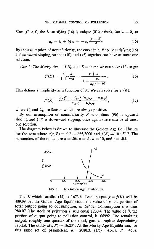
The diagram below is drawn to illustrate the Golden Age Equilibrium for the case where u(c, P) = c1/z - P1.1/5000 and f(K) = 10 * K112. The parameters of the model are a = .06, b = .I, d = 10, and r = .05.

Consumption

FIG. 1. The Golden Age Equilibrium.

The K which satisfies (14) is 1673.6. Total output y = f(K) will be 409.09. At the Golden Age Equilibrium, the value of 01, the portion of total output going to consumption, is .68462. Consumption c is thus 280.07. The stock of pollution P will equal 1230.4. The value of /3, the portion of output going to pollution control, is .06992. The remaining output, roughly one quarter of the total, goes to replace depreciating capital. The utility U(C, P) = 16.234. At the Murky Age Equilibrium, for this same set of parameters, K = 2080.3, f(K) = 456.1, P = 4561,


CY = .7264, /I = 0, and c = 331.3. Here utility u(c, P) = 16.08, is less than it is at the Golden Age. In other situations this ordering could be reversed.

To summarize, there can be no more than two K, P equilibrium pairs that satisfy the necessary conditions for optimality. The no-depollution- expenditure equilibrium will exist if the K value satisfying (9b) and (17) is greater than the K defined in (14), the Golden Age Equilibrium K. The Golden Age Equilibrium will exist if (14) can be satisfied and if the c simultaneously solving (10) and (15) lies between 0 and f(K) -- aK. Further, if capital is fixed at K, the optimal path is going directly from P(0) to the P of the Golden Age Equilibrium. This last result can be generalized. For any choice of fixed K, the optimal path is going directly to the level of P for which up = -u, . ((r + b)/d).

We conjecture, although we have not yet been able to prove, that starting with any initial stocks for K and P the optimal path will in time get arbitrarily close to an equilibrium. The analysis of optimal paths from arbitrary K(O), P(0) is extremely complicated. We have proved our conjecture for a simple example in which the disutility of pollution is linear and separable.”

Model II. Pollution Control Through Choice of Production Process

We now present a model for a pollutant which as a stock enters the welfare function with a negative marginal utility, but as a flow enters the production function with a positive marginal product. The insecticide D.D.T. is a good real-life example of a dual-roled pollutant of this type.

For simplicity, we assume that once the pollutant has been created, it can only be reduced by natural decay. To avoid irrelevant complications, we take labor to be the single scarce productive resource. Thus the policy problem in this model is the choice of production procedures-this choice is exercised by dividing labor between the consumption good sector and the pollutant sector.

The objective function is the same as before. To facilitate exposition, we shall assume that the utility function has a specific form, that it is separable in consumption and pollution, so that

u(c, P) = g(c) - h(P). (18)

We assume that g’(O) = -t co, g’ 3 0, g” < 0, h’(0) = 0, h’ >, 0, and h” > 0.

5 This proof as well as a comparison showing that the optimal path is little superior to a “rule-of-thumb” path using the golden age expenditure proportions throughout is given in Zeckhauser, Keeler, and Spence [Ill.


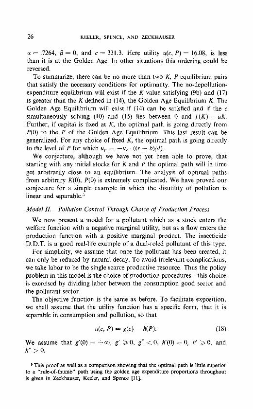
Labor L, the only factor of production, is in tied supply. Some labor L, is allocated to the production of the pollutant through its production function j(L,). We assume that j’(L,) > 0, j”(L,) < 0 and 0 < L < L.

The rest of the labor supply L - & is allocated to the production of the consumption good. The pollutant, serving as an intermediate good, is the other input to the consumption good’s production function. That function is

c = w - L, , j(L)), (19)

where j(L,) gives the primary flow of the produced pollutant. A positive amount of the labor input, but not of the pollutant input, is needed for any production of the good. It is clear that this function can be reduced to c = f(L,), with L an unspecified parameter lurking in the background. The shape off(L,) is shown in Figure 2.‘j

c=f(L,)

c7‘\\

I

r L Ll

FIG. 2. Production as a function of labor allocated to pollutant production.

Beyond the point f: of maximum production, increased labor to pollutant production reduces the output of the consumption good, because the loss from the reduced direct labor input outweights the gain from increased pollutant input.

Necessary conditions for optimality. The modified Hamiltonian expression, with the e-pt dropped, is

H = g(fG)) - W) + +4L,) - W + q(L - Ld + sL, . (20)

Here q and s are time-dependent nonnegative multipliers corresponding to the constraints on L, . It is clearly inefficient to devote more than E to pollutant production, since pollution is valued nonpositively. Hence, L, < L, and q will be identically zero. That the multiplier s may be positive is an important aspect of the problem.

The instantaneous optimal value for L, , given the shadow price rr, can be derived from

HLI = g’f’ + mj’ + s = 0, with s > 0 and sL, = 0. (21)

6 If F12 > 0, then f” < 0 throughout.


Consider first the case where L, > 0 and hence s = 0. If r = 0, clearly L, = Il.

We can differentiate (21) to obtain

dL .I

-=- dr (g”ff2 + j’f” +,j”H) ’ (22)

This will be positive whenever j” is “small” relative to g” and f”. In what follows we assume

Since f(L,) > 0 at L, = 0, g’(f(0)) is finite. Thus, for s = 0, there is a lower bound on 7~ given by

For n < ii, Eq. (21) defines s, which becomes positive. In this region, L, is zero.

Dynanzic Conditions. The perfect foresight condition is

7i = (q + b) 7T + h’. (25)

As before, we adopt the phase-diagram approach to solution. The line 7i = 0 passes through the origin and has the negative slope -(q + b)/h”(P). The line p = 0 is defined by P = j(L.,(n))/b. Since b > 0, and j’ > 0, the slope of P = 0 is positive. Thus the two lines have a unique intersection, and there exists an optimal path through the point of intersection. For a proof of this kind of result, see Arrow [l]. As before, the optimal

Optimal Path \

+=o,

AP

PO F;=o

n no f IT*

FIG. 3. Phase diagram for Model II.

’ This seems reasonable for D.D.T., since the resources devoted to its production are so small relative to total agricultural production resources.


initial level of 7r is the value on the optimal path corresponding to the initial level P,, of the pollutant.

The interesting aspects of this problem may now be examined. Let P be the abscissa of the point of intersection of the optimal path with the line 7~ = ii. If P,, > P, the optimal policy consists of setting L, = 0, and leaving it there until the natural decay of P reduces the level of the pollutant to P. Then it gradually increases L, while maintaining P < 0, until the optimal stationary point (x*, P*) is approached. At the stationary point (which will never quite be reached), L, < L.

The model points out that just as it is not optimal to ignore the pollution problem, neither is it optimal to ban the flow of the pollutant forever. It may not even be optimal to ban its use now; whether it is depends on the current level of the stock of the pollutant. There are at least two policy problems here. One is to determine the critical level P below which production of the pollutant should be allowed. The second is one of implementation-limiting the use of the pollutant to the required amount. In general, simple policies like complete permissiveness and complete abolition are easiest to administer. But the economic losses from opting for a simple policy, when others are feasible, may be large.

The rate of decay b is the crucial factor in determining the level P beyond which the use of the pollutant should be banned. In the case of D.D.T., b is very small, so that banning its use altogether might not be far from the optimal policy. As an experiment, let us allow b to rise.8 On the optimal path in (n-, P) space, the direction of motion is (+, p). The derivative C//C&(+, P) = (.rr, -P). On the upper part of the path, this represents a clockwise twist as b increases. Even if the optimal stationary point (n*, P*) were the same, P would have to rise. But, in addition, the line 7i = 0 is steeper and the line i) = 0 is flattened out. Hence the stationary 7~~ rises which makes the stationary L,* rise. If b is raised far enough, P* must fall, but for small increases in intermediate values of b, the value of P* may rise or fall. To sum up, the higher the rate of decay, the higher is the level at which the pollutant’s use is banned, and the less likely is the policy of banning to be optimal.

Results and Extensions

The two models we discussed produced quite different results. The differences suggest that there are no general rules for dealing with the

*This might be accomplished by the development of bio-degradable pesticides. The research on juvenile hormone pesticides has a different impetus. These are more specific, i.e., only damaging to particular insects, and are effective in smaller quantities. In terms of our model, h(P) is reduced by their first property, and z is reduced by the second, because of the increase in FL .


pollution problem, and that there is no single model that is sufficiently well defined to give results of interest without further specification. Never- theless, we believe that our models can be extended to relate to a variety of pollution problems that maintain the spirit of the assumptions set out below:

Flow of pollution controlled through

Pollution reduction Choice of production process process

As byproduct Pollutant of production Model I -

enters model Produced as

intermediate good - Model II

Consider river pollution. If factories treat their own effluents, they will be adopting a more expensive production process. Pollutant flow reduction is achieved at a cost in productivity; the tools of Model II apply. On the other hand, if the pollutants are dumped but the river is treated, say through aeration, then the logical structure is that of Model I.

The paper-making industry affords a good illustration of the upper right-hand box of the table. That industry offers a choice of productive processes, the less organic residue that is dumped for a particular process, the less effluent it is in terms of cost per unit of paper produced. The tools of Model II can be applied to this, or any, situation in which a choice must be made among productive processes, the ones which are more productive producing as well greater pollutant byproduct.

The models can be applied to problems involving more than pure production processes. With nonreturnable bottles, the “producers” of drinks in the consumers’ refrigerators have higher costs (recognizing convenience as a cost) with the returnable bottle production process, but this process causes less pollution. Although the costs of disposing of nonlittered bottles is low, littered bottles are expensive to remove, in many cases prohibitively so. Thus, applying Model II (to them) may be reasonable. A ban on littered bottles may be appropriate depending on the aesthetic costs.g Another example is traffic congestion; it can be viewed as a by-product of transportation.

Future investigations should relax three assumptions of our models. (1) Capital should be employed in the pollution reduction sector.

0 The marginal disutility of litter may be decreasing, K’(P) < 0, in which case, rather than our marginal approach, zero or total removal strategies may be appropriate.


(2) Technological progress should be considered, particularly in the pollutant-removal sector where progress can and should be anticipated over the short-term future. (3) The labor supply should be treated as an endogenous variable to acknowledge explicitly the relationship between population growth and pollution, and to illustrate the possible need for methods of population control.

CONCLUSION

If strongly expressed social and political concerns reflect nonoptimal situations, our society is currently functioning with a pollution level well in excess of the optimal equilibrium. Too much emphasis, it is believed, has been placed on building the capital stock and on maintaining a high level of consumption. The overwhelming presence of external disecono- mies in an unhindered market situation has led to a nonoptimal outcome. What is needed is some form of centralized coordination to correct a situation which presents inappropriate incentives. Such coordination might be carried out through effluent charges, a market for pollution rights, or perhaps through direct control.

Our models point out that, in general, drastic measures are not called for. In many situations, overreaction is a significant danger. What is called for is a controlled movement toward optimal paths. Unfortunately, political realities may proscribe policies which call for incremental changes in behavior. Banning may be possible in places where reducing would require an infeasible amount of administration. The radical policy, or perhaps no policy at all, may be best among those that can be implemented.

The real-life role of the economist is not only to identify paths of optimality, as we have done, but also to suggest practical ways in which these paths might be approached. It is in this “but also” area where our contributions have been traditionally the weakest.

APPENDIX: OTHER MODELS OF POLLUTION CONTROL

Model III. Generalized Model Presenting Two-State Variable Problems

A general model of pollution control is a full blown two-state variable problem in capital and pollution, in which both the stock and flow of pollution appear in both the production and utility functions, and both capital and current income can be used to reduce the level of flow of the pollutant.


Let K1 represent the part of the capital stock which is devoted to the production of the good, with KS devoted to the reduction of the flow of the pollutant. The fraction of current income devoted to pollution control is /3; its constant productivity is given by d. The problem then is to maximize

.Z

J e-%(c, i’, P) dt, 0

subject to

R=F(K,,P,P)-c---F--K,

Ij = g(K,) - h(K,) - d/3F - bP,

K = Kl -I- Kz , and c > 0, p > 0.

We have had limited success dealing with this general problem at an abstract level. The problem is that with two-state variables P and K the optimal paths are defined by four differential equations in four-dimensional space, and hence, unlike the Ramsey problem, are hard to visualize. (Additional complications arise if the realistic irreversibility conditions &I > -aK, and J& 2 -aK, are imposed.) Progress in analyzing such two-state variable problems would be a significant step forward. The quantities in the model deserve some attention. Situations which fit the general model or any one of its many possible specializations will undoubtedly occur to the reader. We have mentioned several in the paper. In particular, Model I is obtained by setting au/aP = 0, KS = 0, ar;/aP = 0, ayaP = 0.

Model IV. Pollutant Has Utility Impact as a Flow

The objective in this model is to maximize

s

m

u(c, P) ecTt dt, 0

subject to

p = g(K) - W-h), K = IG + K, , and K=f(K,)-c-aK.

Substituting the expression for p in the utility function gives a maximand of

s m u(c, g(K,) - h(K,)) e-rt dt. ”


This problem is equivalent to the one in which the capital stock must be divided between the public and private sectors, the division appearing as well in the utility function. lo This problem, with but one structural difference, has been solved by Professors Arrow and Kurz [2]. The difference is that capital in the public sector K, does not appear in the utility function in their model. It should be said that they were not dealing directly with a pollution problem, but rather with the general problem of the optimal accumulation of capital in the public sector.

Model V. Pollution Model Analogous to the Ramsey Model

The problem is to maximize

.r

m

u(c, P) e-rt dt 0

subject to

L = L, + L, , and P = g(L,) - h(L,).

Here L is the constant labor supply, and L, and L, its allocation between production of the consumption good, and reduction of the pollutant. The problem is of some interest because the formal solution is the exact analog of the simple Ramsey problem, only polluation rather than capital is the one-state variable. The solution of the problem is formally the same as the solution to the Ramsey problem.

Model VI. Exogenous Population Growth

This is a slight variant of Model I, with the population of size L growing at a constant rate n, and utility a function of per capita consumption and total pollution. Let c = C/L, k = K/L.

The maximand is c - u(P) subject to

and

Ji = (1 - 01 - P)f(k) - (a + n) k,

i) = f(K)(l - ,Bd) - bP.

In this case, there is no steady state equilibrium. Because there are decreasing returns to production, as well as positive depreciation, per capita consumption is bounded. Since paths of zero utility are feasible, total pollution must be bounded on any optimal path and hence pollution

lo There may be a problem with the loss of concavity when the substitution is made for P.


cannot increase proportionally with population. Of course, indefinite exponential population growth leads to more serious problems than mathematical intractability.

ACKNOWLEDGMENTS

Professors Henry Jacoby, Thomas Schelling and a referee provided us with helpful comments.

REFERENCES

1. K. J. ARROW, “Applications of Control Theory to Economic Growth,” Reprint No. 95, Institute for Mathematical Studies in the Social Sciences, Stanford Uni- versity, Stanford, Calif. 1968.

2. K. J. ARROW AND M. KURZ, “Public Investment, the Rate of Return, and Optimal Fiscal Policy,” Institute for Mathematical Studies in the Social Sciences, Stanford University, Stanford, Calif. 1968.

3. A. E. BRYSON AND Y. C. Ho, “Applied Optimal Control” (preliminary text), Blaisdell, Waltham, Mass. 1968.

4. R. COURANT, “Differential and Integral Calculus,” Blackie and Son, New York, 1936.

5. A. R. DOBELL AND Y. C. Ho, Optimal Investment Policy: An Example of a Control Problem in Economic Theory, IEEE Trans. Automatic Control, AC-12 (1967), 4-14.

6. M. D. EDEL, “On Silent Springs and Multiple Roots: Cost-Benefit Methods and Environmental Damage,” Working Paper No. 48, Department of Economics, Massachusetts Institute of Technology, Cambridge, Mass., January 1970.

7. M. KURZ, Optimal Economic Growth and Wealth Effects, Infer. Econ. Rev., 9 (1968), 348-357.

8. H. E. RYDER, JR., “Optimal Accumulation in a Two-Sector Economy with Non- shiftable Capital,” (mimeographed),

9. H. E. RYDER, JR., “Optimal Allocation in a Listian Model,” (mimeographed). 10. H. UZAWA, Optimal Growth in a Two-Sector Model of Capital Accumulation,

Reo. Econ. Studies 31 (1964). 11. R. ZECKHAUSER, M. SPENCE AND E. KEELER, “The Optimal Control of Pollution,”

Discussion Paper Number 1, Public Policy Program, Kennedy School of Govern- ment, Harvard University, Cambridge, Mass., June 1970.

Documents

JOURNAL. OF ECONOMIC THEORY 4, 19-34 (19713 Control...JOURNAL. OF ECONOMIC THEORY 4, 19-34 (19713 The Optimal Control of Pollution* EMMETT KEELER, MICHAEL SPENCE, AND RICHARD ZECKHAU~ER