JOURNAL OF COMPUTATIONAL AND APPLIED MATHEMATICS

ELSEVIER Journal of Computational and Applied Mathematics 74 (1996) 71-89

Some large-scale matrix computation problems

Z h a o j u n Bai a' 1, M a r k F a h e y a' 1, G e n e G o l u b b'*' 2

aDepartment of Mathematics, University of Kentucky, Lexington, KY 40506, USA bScientific Computing and Computational Mathematics Program, Computer Science Department, Stanford University,

Stanford, CA 94305, USA

Abstract

There are numerous applications in physics, statistics and electrical circuit simulation where it is required to bound entries and the trace of the inverse and the determinant of a large sparse matrix. All these computational tasks are related to the central mathematical problem studied in this paper, namely, bounding the bilinear form uXf(A)v for a given matrix A and vectors u and v, wheref is a given smooth function and is defined on the spectrum of A. We will study a practical numerical algorithm for bounding the bilinear form, where the matrix A is only referenced through matrix-vector multiplications. A Monte Carlo method is also presented to efficiently estimate the trace of the inverse and the determinant of a large sparse matrix.

Keywords." Bilinear form; Gaussian quadrature; Trace; Determinant; Matrix inverse; Monte Carlo simulation; Probabil- istic bound

AMS classification: 65F 10

1. Introduction

The central problem studied in this paper is to estimate a lower bound L and/or an upper bound U, such that

L <<. u T f ( A ) v <~ U, (1)

where A is a n × n given real matrix, u and v are given n-vectors, and f is a given smooth function and is defined on the spectrum of the matrix A. For example, if A is an n x n nonsingular matrix,

* Corresponding author. a The authors were supported in part by an NSF grant ASC-9313958 and in part by an DOE grant DE-FG03-

94ER25219 via subcontracts from University of California at Berkeley. Fahey is also supported by a fellowship from Center for Computational Sciences, University of Kentucky.

2 The work of this author was in part supported by NSF under grant CCR-9505393.

0377-0427/96/$15.00 © 1996 Elsevier Science B.V. All rights reserved PII S 0 3 7 7 - 0 4 2 7 ( 9 6 ) 0 0 0 1 8 - 0

72 Z. Bai et al./Journal of Computational and Applied Mathematics 74 (1996) 71-89

f(2) = 1/2, and u = v = ei, the ith column of the identity matrix I, then uVf(A)v = (A-')u. The problem (1) is to bound the ith diagonal element of the inverse of the matrix A. If we take the sum of all diagonal elements of the inverse of the matrix A, then a related problem is to estimate bounds on the trace of the inverse of A, tr(A-1). Later, we will see that estimating bounds of the determinant det(A) of A is also a related problem.

When the matrix size n is small, say n ~< 200, we can compute the quantity uTf(A)v explicitly by using dense matrix computation methods [8]. In general, such methods may require (~'(n 2) memory storage and C(n 3) floating point operations. Therefore, when n is large, it is impractical to compute u ~ f(A)~ explicitly. In this paper, we will study numerical methods in which the matrix in question is only referenced in the form of matrix-vector products. Because of this feature, the methods are well-suited for large sparse matrices or large structured dense matrices for which matrix-vector products can be computed cheaply. They will normally take about C(3n + ~:) words of memory and C(jv) floating point operations, where x is the required memory for storing the matrix and/or forming matrix-vector products, v is the cost of matrix-vector product and j is the number of iterations.

Using variational principles, Robinson and Wathen have studied a special case of the problem (1), namely, bounding the entries of the inverse of a matrix [18]. Golub, Meurant and Strakos have studied the problem (1) when the matrix A is symmetric positive definite [6, 7]. They closely examined the application of their approach for bounding the entries of the inverse of a matrix. Quadrature rules, orthogonal polynomial theory and the underlying Lanczos procedure are the tools used in their approach.

In this paper, we will follow the work in [-6, 7] and further develop it in the following aspects. First, we will discuss some practical implementation issues of algorithms. Second, we will show how to use the proposed algorithms for bounding the quantities (A- 1)i j, tr(A- 1) and det(A), where the matrix A is not necessarily symmetric positive definite. Third, we will present a Monte Carlo approach for estimating the quantities tr(A-1) and det(A), which significantly reduces the com- putational cost and obtain a truly practical method for dealing with large-scale matrices.

A number of applications of problem (1) have been discussed in [-7], such as estimating the accuracy of the CG method for solving large linear systems of equations and solving constraint quadratic optimization. New sources of applications are in the fields of fractals [19, 12, 22] and lattice Quantum Chromodynamics (QCD) [-10, 20, 2]. In fact, the QCD applications are the main motivation of our current studies. It is said that a large fraction of the world's supercomputer time is being consumed by physicists in lattice QCD to meet their stringent numerical computation demands. Some of their computational kernels are focused on solving large scale matrix computa- tion problems, such as computing the trace of the inverse and the determinant of matrices of order millions. Numerical analysts have been advised for years that these quantities are too numerically sensitive to compute. Computational physicists, with little or no help from numerical analysts, have developed numerical techniques to compute these quantities. In this paper, we aim to develop practical numerical techniques to tackle these difficult matrix computation problems that have eluded us for years. We believe that our approaches are more efficient than those currently being used by practitioners.

The rest of this paper is organized as follows: In Section 2, we review the basic idea of algorithms presented in [-6, 7], and discuss a number of practical implementation issues of algorithms. Section 3 discusses the applications of the approaches for estimating the bounds of the entries and

Z Bai et al./Journal of Computational and Applied Mathematics 74 (1996) 71-89 73

trace of the inverse of a matrix and the determinant . A Monte Carlo approach and the related confidence bounds are studied in Section 4. Section 5 collects some numerical results. This paper is concluded with open problems and future work.

2. Basic algorithm

In this section, we first review the approach presented in [-6, 7] for estimating the quant i ty uTf(A)v and then discuss some implementa t ion issues. We will assume that the matrix A is symmetric positive definite. In the next section, we will show how to use these algori thms to bound the entries of the inverse of a matrix A, tr(A-1) and det(A), where A is not necessarily symmetric positive definite.

2.1. Main idea

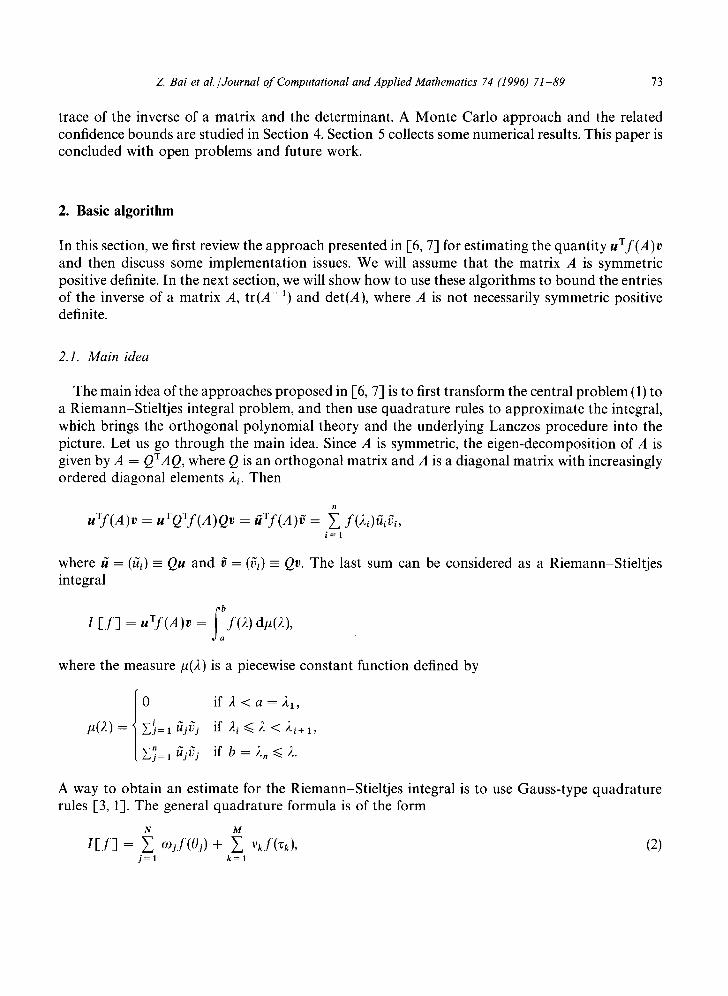
The main idea of the approaches proposed in [-6, 7] is to first t ransform the central problem (1) to a Riemann-Stiel t jes integral problem, and then use quadrature rules to approximate the integral, which brings the or thogonal polynomial theory and the underlying Lanczos procedure into the picture. Let us go th rough the main idea. Since A is symmetric, the eigen-decomposi t ion of A is given by A = QTAQ, where Q is an or thogonal matrix and A is a diagonal matrix with increasingly ordered diagonal elements 2i. Then

uTf(A)v = uTQTf(A)Qv = t~Tf(A)t~ = ~ f(2,)(t,~, i = 1

where t~ = (ui) - Qu and f = 07i) - Qv. The last sum can be considered as a Riemann-Stiel t jes integral

I I f ] = uXf(A)v = f l f ( 2 ) dp(2),

where the measure p(2) is a piecewise constant function defined by

= t 0

Z ! = 1 ~tjVj

L Y j= 1 ajv)

if 2 < a = 2 1 ,

if 2 i ~< 2 < ,~i+1,

if b = 2, ~< 2.

A way to obtain an estimate for the Riemann-Stiel t jes integral is to use Gauss-type quadrature rules [-3, 1]. The general quadra ture formula is of the form

N M I [ f ] = ~ (ojf(Oj) + ~" Vkf(Zk), (2)

j = l k = l

74 Z. Bai et al. /Journal of Computational and Applied Mathematics 74 (I 996) 71-89

where the weights {Oj> and { vk) and the nodes { Qj} are unknown and to be determined. The nodes {Q) are prescribed. The integration error (remainder) is

WI = s b.f@) d/G) - Kfl. a

If A4 = 0, then it is the well-known Gauss rule. If A4 = 1 and z1 = a or z1 = b, it is the Gauss-Radau rule. If A4 = 2 and 21 = a and z2 = b, it is the Gauss-Lobatto rule. The sign of R [f] determines whether the quadrature formula I [f] is a lower bound (if R [f] > 0) or an upper lower bound (if R[f] < 0) of the quantity uTf(A)u.

We will focus on the case u = u in the following discussion. In this case, the measure p(A) is a positive increasing piecewise constant function. We note that the case u # u can be reduced to the case u = u by the polarization expression

UTf(& = $(YTf(4Y - z’f(A)z), (3)

wherey=rc+uandz=u-u.

2.2. Basic algorithm

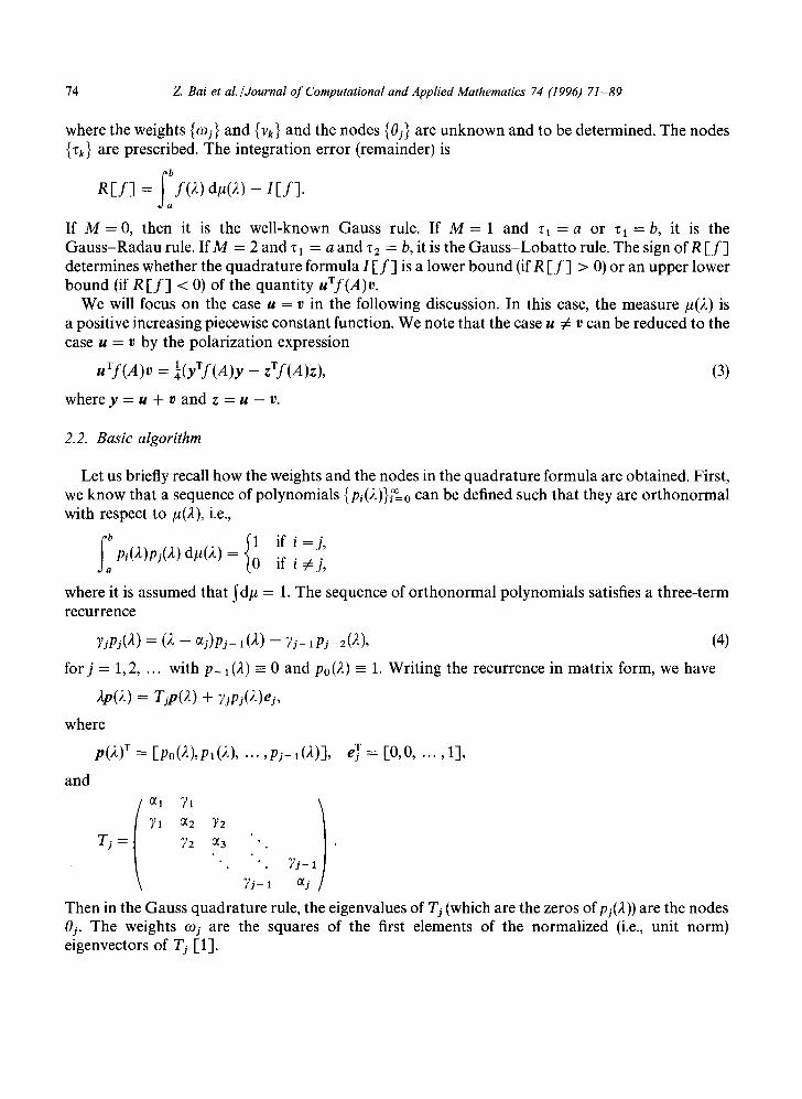
Let us briefly recall how the weights and the nodes in the quadrature formula are obtained. First, we know that a sequence of polynomials {pi(A)}g, can be defined such that they are orthonormal with respect to p(A), i.e.,

s b

pi(A dp(A) = ’ if ’ =” a 0 if i #j,

where it is assumed that Jdp = 1. The sequence of orthonormal polynomials satisfies a three-term recurrence

YjPjtA) =(A - aj)Pj-l(a) -Yj-lPj-2(Ah (4)

forj = 1,2, . . . with p-i(A) z 0 and p,(A) = 1. Writing the recurrence in matrix form, we have

and

Tj =

a1 Yl

Yl a2 Y2

Y2 a3 *..

*.* .*

. Yj-1

"t-1 aj

Then in the Gauss quadrature rule, the eigenvalues of Tj (which are the zeros Of pi(A)) are the nodes 8j. The weights Oj are the squares of the first elements of the normalized (i.e., unit norm) eigenvectors of Tj [l].

Z. Bai et al./Journal of Computational and Applied Mathematics 74 (1996) 71-89 75

In the G a u s s - R a d a u and G a u s s - L o b a t t o rules, the nodes {02}, {Zk} and weights {coj}, {v j} come from eigenvalues and the squares of the first elements of the normalized eigenvectors of an adjusted tr idiagonal matr ix of Tj,, which has the prescribed eigenvalues a and/or b, i.e., a and/or b are roots of the polynomial pj+ ~ (2) [6].

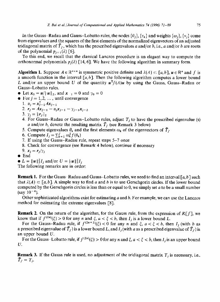
To this end, we recall that the classical Lanczos procedure is an elegant way to compute the o r thonormal polynomials p2(2) [14, 6]. We have the following algori thm in summary form.

Algorithm 1. Suppose A e ~"×" is symmetric positive definite and 2(A) ~ [a ,b] , u ~ ~ " and f is a smooth function in the interval [a, b]. Then the following algori thm computes a lower bound L and /or an upper bound U of the quant i ty u T f ( A ) u by using the Gauss, G a u s s - R a d a u or G a u s s - L o b a t t o rules. • Let x0 = u~ II u II 2, and x_ 1 = 0 and 70 = 0 • For j = 1, 2, . . . , until convergence

1. O~j = x T - 1 A x j - 1

2. rj = A x j _ ~ - o~jxj_~ - y j - ~ x j - 2

3. ~j = [Irjll2 4. For G a u s s - R a d a u or G a u s s - L o b a t t o rules, adjust Tj to have the prescribed eigenvalue (s)

a and/or b, denote the resulting matrix 2~j, (see Remark 3 below) 5. C ompu te eigenvalues Ok and the first elements Ok of the eigenvectors of Tj, 6. C ompu te Ij = E~'= 1 o2f(Ok) 7. If using the G a u s s - R a d a u rule, repeat steps 5-7 once 8. Check for convergence (see Remark 4 below), cont inue if necessary 9. x~ = rj /Tj

• End • L = Ilu1122I~ and/or U = IlullzzI~ The following remarks are in order:

Remark 1. For the G a u s s - R a d a u and G a u s s - L o b a t t o rules, we need to find an interval [a, b] such that 2(A) c I-a, b]. A simple way to find a and b is to use Gerschgorin circles. If the lower bound computed by the Gerschgorin circles is less than or equal to 0, we simply set a to be a small number (say 10-4).

Other sophisticated algori thms exist for estimating a and b. For example, we can use the Lanczos me thod for est imating the extreme eigenvalues [8].

Remark 2. On the return of the algori thm, for the Gauss rule, from the expression of R [ f ] , we know that if f~2,)(¢) > 0 for any n and 4, a < ~ < b, then Ij is a lower bound L.

For the G a u s s - R a d a u rule, if f~2,+1)(~) < 0 for any n and 4, a < ~ < b, then Ij (with b as a prescribed eigenvalue of Tj,) is a lower bound L, and Ij (with a as a prescribed eigenvalue of T~,) is an upper bound U.

For the G a u s s - L o b a t t o rule, if f~2,j(~) > 0 for any n and 4, a < ~ < b, then Ij is an upper bound U.

Remark 3. If the Gauss rule is used, no adjus tment of the tr idiagonal matrix Tj is necessary, i.e., •, = Tj.

76 Z. Bai et aL /Journal of Computational and Applied Mathematics 74 (1996) 71-89

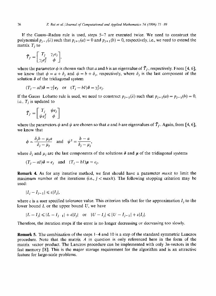
If the Gauss -Radau rule is used, steps 5-7 are executed twice. We need to construct the polynomial pj+ 1(2) such that pj+l(a) = 0 and pj+ 1 (b) = 0, respectively, i.e., we need to extend the matrix Tj to

~j e~

where the parameter t k is chosen such that a and b is an eigenvalue of Tj,, respectively. F rom [4, 6], we know that ~ = a + 6j and ~ = b + 6j, respectively, where 6j is the last component of the solution 5 of the tridiagonal system

(Tj a I )6 2 (Tj b I )5 7~ej. - - = 7j ej o r - - -~

If the Gauss -Loba t to rule is used, we need to construct pj+ 1(2) such that pj+ l(a) = pj+ l(b) = 0, i.e., Tj is updated to

1 where the parameters ~b and ~ are chosen so that a and b are eigenvalues of Tj,. Again, from [4, 6], we know that

(9 - 6jb - p ja and 11/2 __ b - a 6j - pj 6j - ~j '

where 6j and pj are the last components of the solutions 5 and p of the tridiagonal systems

(Tj - a I )~ = ej and (Tj - bI)la = ej.

Remark 4. As for any iterative method, we first should have a parameter maxi t to limit the maximum number of the iterations (i.e., j < maxit) . The following stopping criterion may be used:

IIj - I j -a [ ~ e[Ij[,

where e is a user specified tolerance value. This criterion tells that for the approximation I j to the lower bound L or the upper bound U, we have

I Z - - I j l < < . l L - I j - l l + e l l j l or I U - I j I ~ < I U - I j - I I + e I I j [ .

Therefore, the iteration stops if the error is no longer decreasing or decreasing too slowly.

Remark 5. The combination of the steps 1-4 and 10 is a step of the standard symmetric Lanczos procedure. Note that the matrix A in question is only referenced here in the form of the matr ix-vector product. The Lanczos procedure can be implemented with only 3n-vectors in the fast memory [8]. This is the major storage requirement for the algorithm and is an attractive feature for large-scale problems.

Z Bai et al./Journal of Computational and Applied Mathematics 74 (1996) 71-89 77

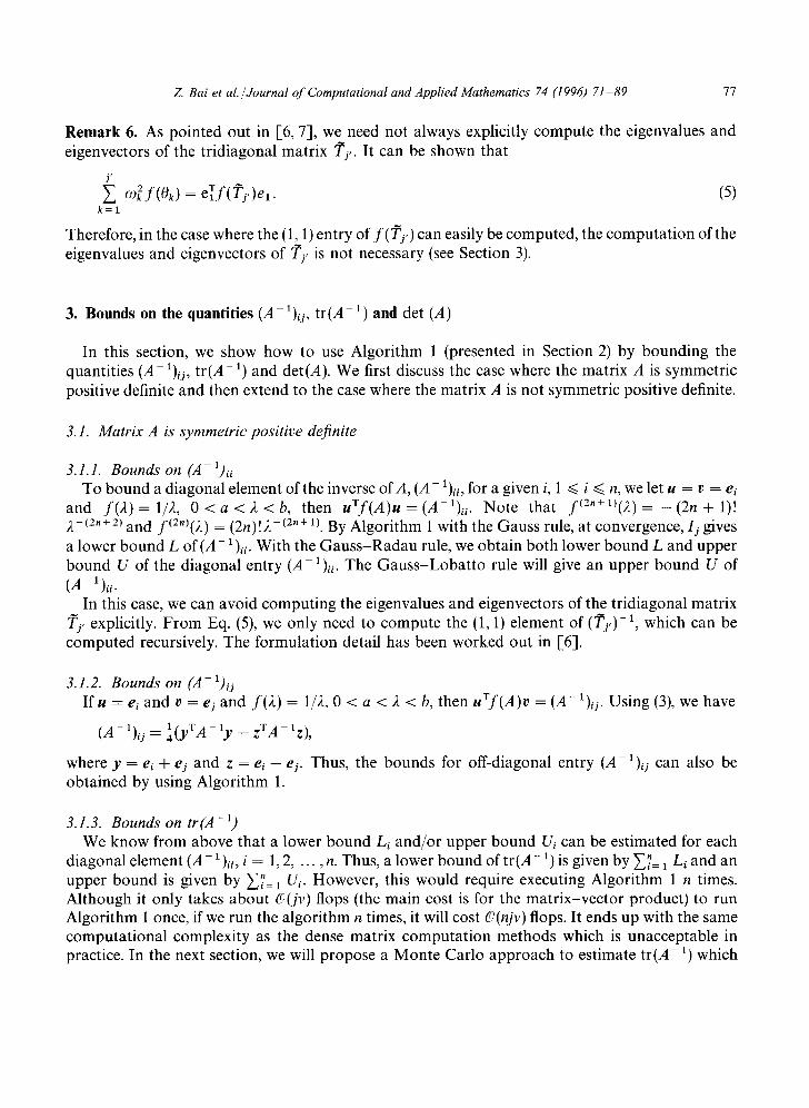
Remark 6. As pointed out in [6, 7], we need not always explicitly compute the eigenvalues and eigenvectors of the tr idiagonal matrix Tj,. It can be shown that

j '

a~2 f (Ok) = e l f ( T j , ) e l . (5) k = l

Therefore, in the case where the (1, 1) entry of f (Tj , ) can easily be computed, the computa t ion of the eigenvalues and eigenvectors of Tj, is not necessary (see Section 3).

3. Bounds on the quantities (A-1)ij, tr(A-1) and det (A)

In this section, we show how to use Algori thm 1 (presented in Section 2) by bounding the quantit ies (A- 1)~j, t r (A- 1) and det(A). We first discuss the case where the matrix A is symmetric positive definite and then extend to the case where the matrix A is not symmetric positive definite.

3.1. Matr ix A is symmetr ic pos i t ive definite

3.1.1. Bounds on ( A - 1 ) u To bound a diagonal element of the inverse of A, (A- 1)u, for a given i, 1 ~< i ~< n, we let u = v = e~

and f (2 ) = 1/2, 0 < a < 2 < b, then u T f ( A ) u = (A-X)i i . Note that f~2"+1)(2) = - (2n + 1)! 2-(2, + 2) and f~2")(2) = (2n)!2-12, + 1). By Algori thm 1 with the Gauss rule, at convergence, Ij gives a lower bound L of (A- 1),. With the G a u s s - R a d a u rule, we obtain both lower bound L and upper bound U of the diagonal entry (A- 1)u. The G a u s s - L o b a t t o rule will give an upper bound U of ( a - 1 ) i i .

In this case, we can avoid comput ing the eigenvalues and eigenvectors of the tr idiagonal matrix Tj, explicitly. F r o m Eq. (5), we only need to compute the (1, 1) element of (Tj,)- 1, which can be computed recursively. The formulat ion detail has been worked out in [-6].

3.1.2. B o u n d s on (A-1) i i I f u = ei and r = ej and f (2 ) = 1/2, 0 < a < 2 < b, then u V f ( A ) v = (A -1 ) i j . Using (3), we have

(A - 1)i.j = a(yT A - Xy __ zTA - lZ) '

where y = ei + ej and z = e ~ - ej. Thus, the bounds for off-diagonal entry (A-1)~ can also be obtained by using Algori thm 1.

3.1.3. Bounds on tr(A -1 ) We know from above that a lower bound Li and/or upper bound Ui can be est imated for each

diagonal element ( A - 1)u, i = 1, 2, . . . , n. Thus, a lower bound of t r (A- 1) is given by ~ ' = 1 Li and an upper bound is given by y'~'= 1 U/. However, this would require executing Algori thm 1 n times. Al though it only takes about (9(jr) flops (the main cost is for the mat r ix-vec tor product) to run Algori thm 1 once, if we run the a lgori thm n times, it will cost (9(njv) flops. It ends up with the same computa t iona l complexity as the dense matrix computa t ion methods which is unacceptable in practice. In the next section, we will propose a Monte Carlo approach to estimate t r(A-1) which

78 Z. Bai et aL /Journal of Computational and Applied Mathematics 74 (1996) 71-89

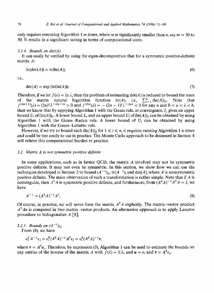
only requires executing Algori thm 1 m times, where m is significantly smaller than n, say m = 30 to 50. It results in a significant saving in terms of computa t ional costs.

3.1.4. Bounds on det(A) It can easily be verified by using the eigen-decomposi t ion that for a symmetric positive-definite

matrix A:

ln(det(A)) = tr(ln(A)), (6)

i . e . ,

det(A) = exp (tr(ln(A))). (7)

Therefore, if we let f (2 ) = In 2, then the problem of estimating det (A) is reduced to bound the trace of the matrix natural logar i thm function ln(A), i.e., ~ ' = l ( l n ( A ) ) , . Note that f ( 2 n + 1)(/~) = (2n)!)~-(zn+ 1) > 0 and f ( 2 n ) ( ) ~ ) = _ (2n - 1)!• -(2n) < 0 for any n and 0 < a < 2 < b, then we know that by applying Algori thm 1 with the Gauss rule, at convergence, Ij gives an upper bound Ui of(ln(A))ii. A lower bound Li and an upper bound Ui of(ln(A))u can be obtained by using Algori thm 1 with the G a u s s - R a d a u rule. A lower bound of Ui can be obtained by using Algori thm 1 with the G a u s s - L o b a t t o rule.

However, if we try to bound each (ln(A))u for 1 ~< i ~< n, it requires running Algori thm 1 n times and could be too costly to use in practice. The Monte Carlo approach to be discussed in Section 4 will relieve this computa t ional burden in practice.

3.2. Matrix A is not symmetric positive definite

In some applications, such as in lattice QCD, the matrix A involved may not be symmetric positive definite. It may not even be symmetric. In this section, we show how we can use the techniques developed in Section 2 to bound (A- 1)ij, tr(A - 1), and det(A), where A is nonsymmetr ic positive definite. The main observat ion of such a t ransformat ion is rather simple. Note that if A is nonsingular, then ArA is symmetric positive definite, and furthermore, from (ATA) - 1ATA = I, we have

A - 1 = (ATA) - XAT" (8)

Of course, in practice, we will never form the matrix ATA explicitly. The mat r ix-vec tor product ATAx is computed in two mat r ix-vec tor products. An alternative approach is to apply Lanczos procedure to bidiagonalize A [8].

3.2.1. Bounds on (A-1)ij F r o m (8), we have

eTA- lei = e~(ATA)- 1ATei = eT(ATA) - IV,

where v = ATej. Therefore, by expression (3), Algori thm 1 can be used to estimate the bounds on any entries of the inverse of the matrix A with f (2 ) = 1/2, and u = ei and v = ATej.

Z Bai et al./Journal of Computational and Applied Mathematics 74 (1996) 71-89

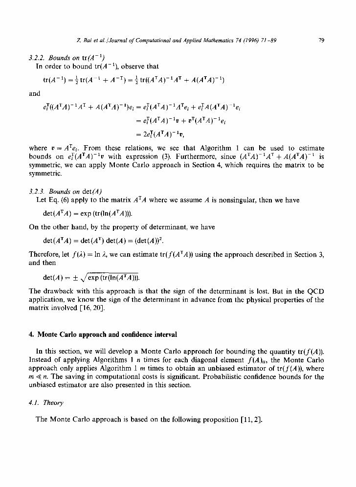
3.2.2. Bounds on t r ( A - 1) In order to bound tr(A-1), observe that

1 tr(A- ~ + A-T) _ 1 tr((AVA)-1AT + A ( A T A ) - 1 ) tr(A- 1) = ~

and

79

e~((ATA) - 1AT + A(ATA) - 1)e i = eT(ATA)-1AXel + eTA(ATA) - le i

= eT(ATA) - iV + vT(ATA) - le i

= 2eT(ATA) - iV,

where r = ATei . From these relations, we see that Algorithm 1 can be used to estimate bounds on e T ( A T A ) - l r with expression (3). Furthermore, since ( A T A ) - I A T + A(ATA) -1 is symmetric, we can apply Monte Carlo approach in Section 4, which requires the matrix to be symmetric.

3.2.3. Bounds on det (A) Let Eq. (6) apply to the matrix ATA where we assume A is nonsingular, then we have

det(ATA) = exp (tr(ln(ATA))).

On the other hand, by the property of determinant, we have

det(ATA) = det (A T) det(A) = (det (A))2.

Therefore, let f(2) = In 2, we can estimate t r ( f (ATA) ) using the approach described in Section 3, and then

det(A) = _+ x/exp (tr(ln(ATA))).

The drawback with this approach is that the sign of the determinant is lost. But in the QCD application, we know the sign of the determinant in advance from the physical properties of the matrix involved [-16, 20-1.

4. Monte Carlo approach and confidence interval

In this section, we will develop a Monte Carlo approach for bounding the quantity tr(f(A)). Instead of applying Algorithms 1 n times for each diagonal element f(A)~i, the Monte Carlo approach only applies Algorithm 1 m times to obtain an unbiased estimator of tr(f(A)), where m ,~ n. The saving in computational costs is significant. Probabilistic confidence bounds for the unbiased estimator are also presented in this section.

4.1. Theory

The Monte Carlo approach is based on the following proposition [11, 2].

80 Z. Bai et al./Journal of Computational and Applied Mathematics 74 (1996) 71-89

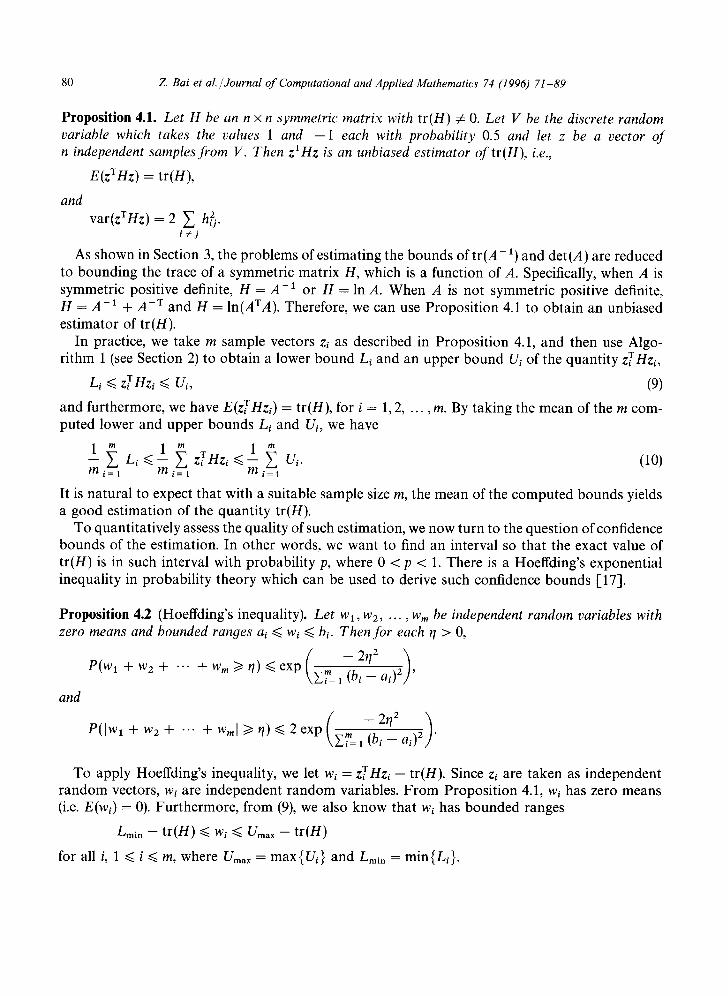
Proposition 4.1. Let H be an n x n symmetric matrix with t r(H) # 0. Let V be the discrete random variable which takes the values 1 and - 1 each with probability 0.5 and let z be a vector oJ n independent samples from V. Then zXHz is an unbiased estimator of tr(H), i.e.,

E(z~Hz) = tr(H),

and var(zXHz) = 2 ~ h 2.

i~ j

As shown in Section 3, the problems of estimating the bounds of t r (A- 1) and det(A) are reduced to bounding the trace of a symmetric matrix H, which is a function of A. Specifically, when A is symmetric positive definite, H = A-1 or H = In A. When A is not symmetric positive definite, H = A-1 + A-T and H = ln(AaA). Therefore, we can use Proposi t ion 4.1 to obtain an unbiased estimator of tr(H).

In practice, we take m sample vectors zi as described in Proposi t ion 4.1, and then use Algo- rithm 1 (see Section 2) to obtain a lower bound L~ and an upper bound Ui of the quanti ty zTHz,

Li <~ z~ H;gi <~ Ui, (9)

and furthermore, we have E(z~Hzg) = tr(H), for i = 1, 2 . . . . . m. By taking the mean of the m com- puted lower and upper bounds Li and Ui, we have

1 ~ Li< 1 ~z.~Hzi<I ~, Ui. (10) mi= 1 mi= 1 mi= 1

It is natural to expect that with a suitable sample size m, the mean of the computed bounds yields a good estimation of the quanti ty tr(H).

To quantitatively assess the quality of such estimation, we now turn to the question of confidence bounds of the estimation. In other words, we want to find an interval so that the exact value of tr(H) is in such interval with probabil i ty p, where 0 < p < 1. There is a Hoeffding's exponential inequality in probabili ty theory which can be used to derive such confidence bounds [17].

Proposition 4.2 (Hoeffding's inequality). Let wl, w2, . . . , Wm be independent random variables with zero means and bounded ranges ai <~ wi <<. hi. Then for each q > O,

P ( w x + w 2 + "" +Wm>~rl)<.exp(,~m ---2q2 ) \ 2 . . , i : 1 (bT---a,) 2 '

and

(wm ~ 2r/2 ) P(Iwx + W2 "+- "'" "}- Wml ) q) ~ 2 exp \2.,i= 1 ( b 7 7 a l ) 2 .

To apply Hoeffding's inequality, we let wl = zTHzi -- tr(H). Since z~ are taken as independent random vectors, wi are independent random variables. F rom Proposi t ion 4.1, w~ has zero means (i.e. E(wi) = 0). Furthermore, from (9), we also know that w~ has bounded ranges

Lmi n -- t r (H) ~< wi <<. Umax -- t r(H)

for all i, 1 ~< i ~< m, where Umax = max{Ui} and Lmin = min{L~}.

Z. Bai et al./Journal of Computational and Applied Mathematics 74 (1996) 71-89 81

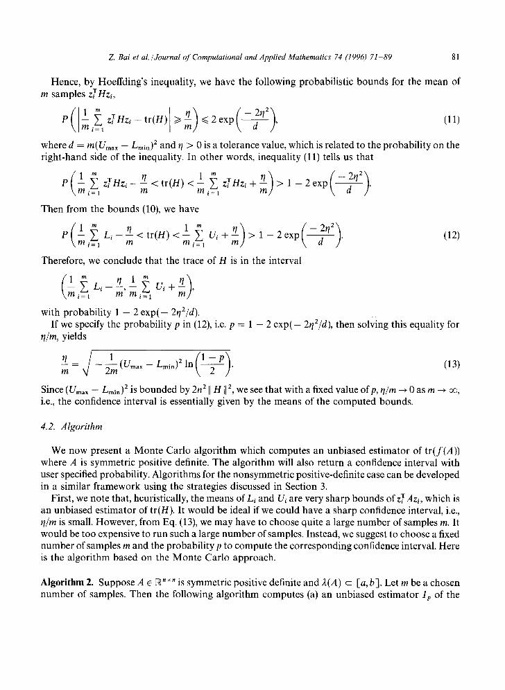
Hence, by Hoeffding's inequality, we have the following probabilistic bounds for the mean of m samples z~Hzi,

P ( I 1 "m~=lz~Hz~- t r (H) / > ~ ) ~ < 2 e x p ( - ~ ) , (11)

where d = m ( U m a x - - L m i n ) 2 and q > 0 is a tolerance value, which is related to the probabili ty on the r ight-hand side of the inequality. In other words, inequality (11) tells us that

P zTHz i _ r/ < tr(H) < - - 7.THzi + > 1 -- 2 exp - - . i = l m m i = 1

Then from the bounds (10), we have

P Li - q-- < tr(H) < Ui + > 1 -- 2 exp . (12) i=l m -~ i=

Therefore, we conclude that the trace of H is in the interval

i = 1 m m i = 1

with probabili ty 1 - 2 e x p ( - 2q2/d). If we specify the probabili ty p in (12), i.e. p = 1 - 2 e x p ( - 2qE/d), then solving this equality for

rl/m, yields

~--- = ~/-- ~m (Umax - Lrnin)2 In ( ~ - ~ ) " m (13)

Since (Umax - L m i n ) 2 is bounded by 2n 2 II H [I 2, we see that with a fixed value of p, film ~ 0 as m ~ ~ , i.e., the confidence interval is essentially given by the means of the computed bounds.

4.2. Algorithm

We now present a Monte Carlo a lgori thm which computes an unbiased est imator of t r ( f (A)) where A is symmetric positive definite. The algori thm will also return a confidence interval with user specified probability. Algori thms for the nonsymmetr ic positive-definite case can be developed in a similar f ramework using the strategies discussed in Section 3.

First, we note that, heuristically, the means of Li and Ui are very sharp bounds of z~Azi, which is an unbiased est imator of tr(H). It would be ideal if we could have a sharp confidence interval, i.e., rl/m is small. However, from Eq. (13), we may have to choose quite a large number of samples m. It would be too expensive to run such a large number of samples. Instead, we suggest to choose a fixed number of samples m and the probabili ty p to compute the corresponding confidence interval. Here is the a lgori thm based on the Monte Carlo approach.

Algorithm 2. Suppose A ~ ~" ×" is symmetric positive definite and 2(A) c [a, b]. Let m be a chosen number of samples. Then the following algori thm computes (a) an unbiased est imator Ip of the

82 Z. Bai et al./Journal o f Computational and Applied Mathematics 74 (1996) 71-89

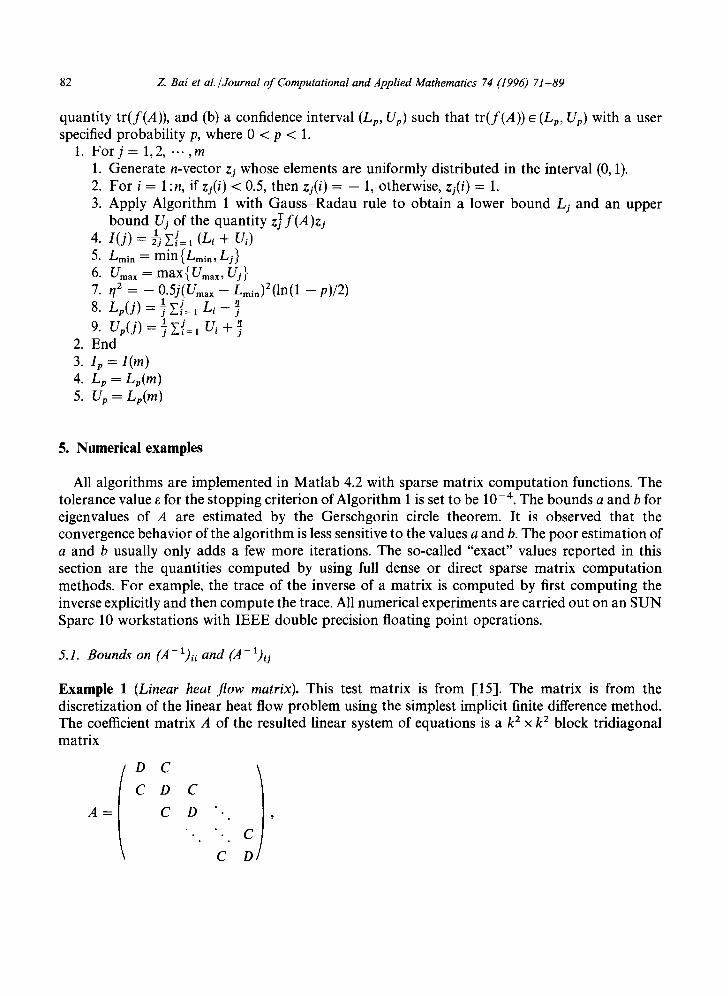
quantity tr(f(A)), and (b) a confidence interval (Lp, Up) such that t r ( f (A)) ~ (Lp, Up) with a user specified probability p, where 0 < p < 1.

1. F o r j = 1,2, ... ,m 1. Generate n-vector zj whose elements are uniformly distributed in the interval (0, 1). 2. For i = l :n, if zj(i) < 0.5, then zj(i) = - 1, otherwise, zj(i) = 1. 3. Apply Algorithm 1 with Gauss -Radau rule to obtain a lower bound Lj and an upper

bound Uj of the quantity z T f ( A ) z j 1 j (Li + Ui) 4. I ( j ) = 73 Y~i = 1

5. Lmi~ = min{Lmln, Lj} 6. Urea, -- max{Urea,, Uj} 7. r/z = - 0.5j(Um~x - Lmin)2(ln(1 -- p)/2)

1 j Li ~1 8. Lp(j) = 7 Ei= l - j 1 j

9. Up(j) =Ty . ,= 1 U i + j 2. End 3. lp = I(m) 4. Lp = Lp(m) 5. Up = Lp(m)

5. Numerical examples

All algorithms are implemented in Matlab 4.2 with sparse matrix computat ion functions• The tolerance value e for the stopping criterion of Algorithm 1 is set to be 10 -4. The bounds a and b for eigenvalues of A are estimated by the Gerschgorin circle theorem. It is observed that the convergence behavior of the algorithm is less sensitive to the values a and b. The poor estimation of a and b usually only adds a few more iterations. The so-called "exact" values reported in this section are the quantities computed by using full dense or direct sparse matrix computat ion methods. For example, the trace of the inverse of a matrix is computed by first computing the inverse explicitly and then compute the trace. All numerical experiments are carried out on an SUN Sparc 10 workstations with IEEE double precision floating point operations•

5.1. Bounds on (A - 1)ii and (A - 1)ij

Example 1 (Linear heat f low matrix). This test matrix is from [15]. The matrix is from the discretization of the linear heat flow problem using the simplest implicit finite difference method. The coefficient matrix A of the resulted linear system of equations is a k 2 × k 2 block tridiagonal matrix

A =

D C

C D C

C D ° ° .

• • ° C

C D

Z. Bai et al./Journal of Computational and Applied Mathematics 74 (1996) 71-89

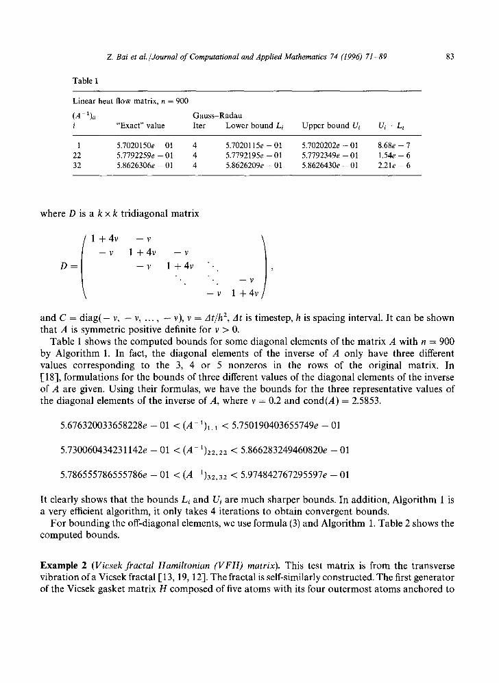
Table 1

83

Linear heat flow matrix, n = 900

(A- 1). i "Exact" value

G a u s s - R a d a u I ter Lower b o u n d Li U p p e r b o u n d Ui U~ - Li

1 5 .7020150e- -01 4 22 5 .7792259e- -01 4 32 5 .8626306e- -01 4

5.7020115e -- 01 5.7020202e -- 01 8.68e -- 7 5 .7792195e- -01 5 .7792349e- -01 1 .54e - -6 5 .8626209e- -01 5 .8626430e- -01 2 . 2 1 e - - 6

where D is a k x k tridiagonal matrix

D =

1 + 4 v - - v

- - v 1 + 4 v v ) 1 + 4 v ".

• . " . - - V

- - v 1 + 4 v

and C = d i a g ( - v, - v, . . . , - v), v = At/h 2, At is timestep, h is spacing interval• It can be shown that A is symmetric positive definite for v > 0.

Table 1 shows the computed bounds for some diagonal elements of the matrix A with n = 900 by Algorithm 1. In fact, the diagonal elements of the inverse of A only have three different values corresponding to the 3, 4 or 5 nonzeros in the rows of the original matrix. In [18-1, formulations for the bounds of three different values of the diagonal elements of the inverse of A are given. Using their formulas, we have the bounds for the three representative values of the diagonal elements of the inverse of A, where v = 0.2 and cond(A) = 2.5853•

5.676320033658228e - 01 < (A-1)l,1 < 5.750190403655749e - 01

5.730060434231142e - 01 < (A-1)22,22 < 5.866283249460820e - 01

5 .786555786555786e-01 < ( A - 1 ) 3 2 , 3 2 < 5.974842767295597e-01

It clearly shows that the bounds Li and Ui are much sharper bounds. In addition, Algorithm 1 is a very efficient algorithm, it only takes 4 iterations to obtain convergent bounds.

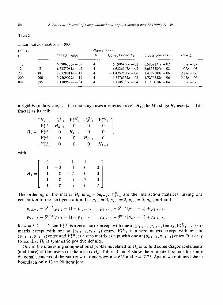
For bounding the off-diagonal elements, we use formula (3) and Algorithm 1. Table 2 shows the computed bounds.

Example 2 (Vicsek fractal Hamiltonian (VFH) matrix). This test matrix is from the transverse vibration o f a Vicsek fractal [13, 19, 12]. The fractal is self-similarly constructed• The first generator of the Vicsek gasket matrix H composed of five atoms with its four outermost atoms anchored to

84

Table 2

Z. Bai et al./Journal of Computational and Applied Mathematics 74 (1996) 71-89

Linear heat flow matrix, n = 900

(A - 1)ij G a u s s - R a d a u i j "Exact" value I ter Lower b o u n d Li Upper bound Ui U i - L i

2 1 6.5906786e - 02 4 6 . 5 9 0 6 4 3 6 e - 0 2 6 . 5 9 0 7 1 7 1 e - 0 2 7.35e - 07 20 21 6 . 6 8 3 7 0 6 1 e - 0 2 4 6 . 6 8 3 6 5 0 7 e - 0 2 6 . 6 8 3 7 5 8 4 e - 0 2 1 . 0 7 e - 0 6

200 181 1 . 6 3 2 8 0 1 1 e - 1 7 4 - 1 . 4 3 5 9 5 0 0 e - 0 6 1 . 4 3 5 9 5 0 0 e - 0 6 2 . 8 7 e - 0 6 200 700 3 . 9 5 0 9 0 2 9 e - 1 9 4 - 1 . 7 2 7 6 3 3 2 e - 0 6 1 . 7 2 7 6 3 3 2 e - 0 6 3 . 4 5 e - 0 6 899 895 1 . 1 1 8 9 5 7 2 e - 0 4 4 1 . 1 1 0 6 3 3 5 e - 0 4 1 . 1 2 7 3 0 1 0 e - 0 4 1 . 6 6 e - 0 6

a rigid b o u n d a r y site, i.e., the first stage uses a toms as its cell Hx, the kth stage H k u s e s (k - 1)th fractal as its cell:

- H k _ l Vk(1)l V(2)r I[(3)T V(4)1 1 - k - 1 V k - ~ -

V(k 1-) 1 Hk - 1 0 0 0

Hk -= Vtk 2-) 1 0 S k - 1 0 0 ,

V(k 3-) 1 0 0 Hk - 1 0

- V(k 4-) 1 0 0 0 Hk - 1

with

- 4 1 1 1 1 ]

1 - 2 0 0 0

H1 = 1 0 - 2 0 0 .

1 0 0 - 2 0

1 0 0 0 - 2

The order n k of the matr ix Hk is n k = 5n k_ 1- Vk q-) 1 are the interact ion matr ices linking one genera t ion to the next generat ion. Let Pl, 1 = 3, P2,1 = 2, P3,1 ~-" 5 , P4, 1 = 4 and

P l , k - 1 = 5 k - 2 ( p l , 1 - - 1) + P l , k - 2 , P2,k-1 = 5 k - 2 ( p 2 , 1 - - 1) + P2,k -2 ,

P3,k-1 = 5 k - 2 ( p 3 , 1 - - 1) + P 3 , k - 2 , P4, k -1 = 5 k - 2 ( p 4 , 1 - - 1) + P4,k -2 ,

for k = 3, 4, . . . . Then Vk~k) l is a zero matr ix except with one at (p 1, k- 1, P2, k- 1 ) entry, Vk~2_ ) 1 is a zero matr ix except with one at (P2.k-l ,Pl,k-1) entry, Vkta2a is a zero matr ix except with one at (P3,k- 1 , P 4 . k - 1) entry and Vk(4-) 1 is a zero matr ix except with one at (Pg.k- 1 ,P3,k- 1) entry. It is easy to see that H k is symmetr ic posi t ive definite.

One of the interesting compu ta t iona l p rob lems related to Hk is to find some diagonal elements (and trace) of the inverse of the matr ix H k. Tables 3 and 4 show the es t imated b o u n d s for some diagonal elements of the matr ix with d imens ion n -- 625 and n = 3125. Again, we ob ta ined sharp b o u n d s in only 13 to 20 i terations.

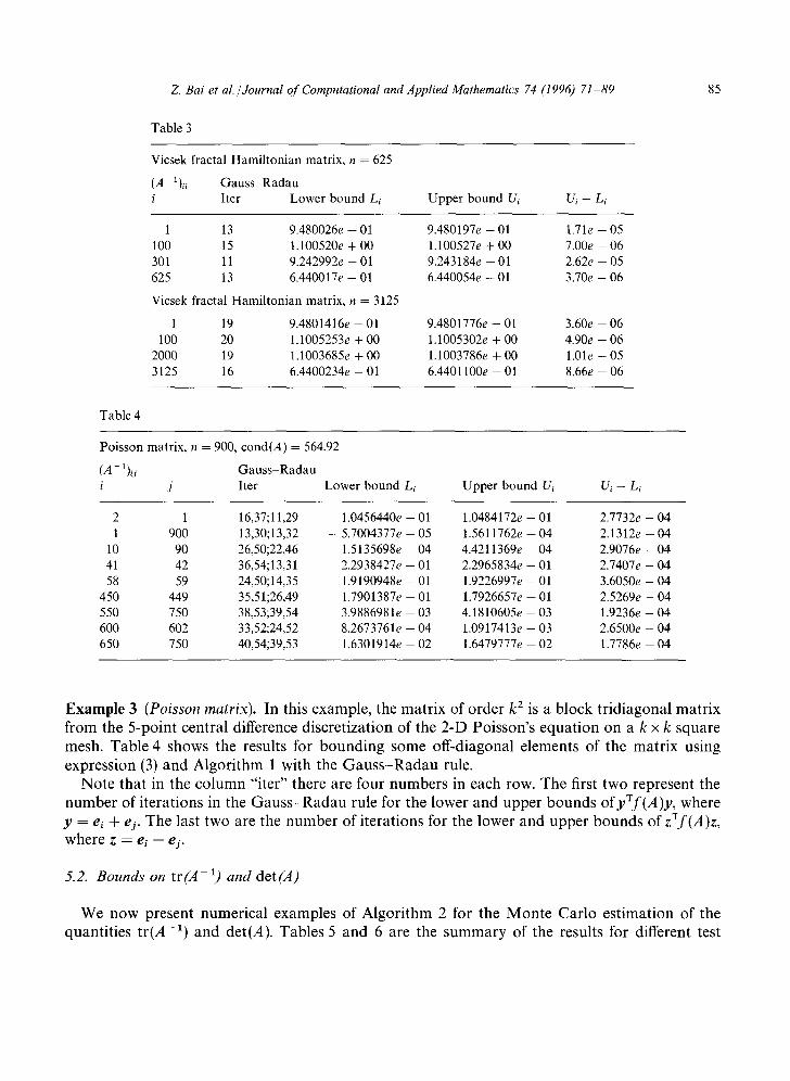
Z. Bai et al./Journal o f Computational and Applied Mathematics 74 (1996) 71-89 85

Table 3

Vicsek fractal Hamiltonian matrix, n = 625

(A 1)i~ Gauss Radau i Iter Lower bound L~ Upper bound Ui Ui - Li

1 13 9 . 4 8 0 0 2 6 e - 0 1

100 15 1.100520e + 00

301 11 9 .242992e - 01

625 13 6 .440017e - 01

Vicsek ffactalHamiltonianmatrix, n = 3125

1 19 9 .4801416e - 01

100 20 1.1005253e + 00

2000 19 1.1003685e + 00

3125 16 6 .4400234e - 01

9 .480197e - 01 1 . 7 1 e - 0 5

1.100527e + 00 7.00e - 06

9 . 2 4 3 1 8 4 e - 0 1 2 . 6 2 e - 0 5

6 . 4 4 0 0 5 4 e - 0 1 3.70e - 06

9 . 4 8 0 1 7 7 6 e - 0 1 3 . 6 0 e - 0 6

1.1005302e + 00 4.90e - 06

1 . 1 0 0 3 7 8 6 e + 0 0 1 . 0 1 e - 0 5

6 . 4 4 0 1 1 0 0 e - 0 1 8 . 6 6 e - 0 6

Table 4

Poisson matrix, n = 900, c o n d ( A ) = 564.92

( A - 1)i. Gauss-Radau J

i j Iter Lower bound Li Upper bound Ui Ui - Li

2 1 16,37;11,29 1 . 0 4 5 6 4 4 0 e - 0 1 1 . 0 4 8 4 1 7 2 e - 0 1 2 . 7 7 3 2 e - 0 4

1 900 13,30;13,32 - 5 .7004377e - 05 1.5611762e -- 04 2.1312e -- 04

10 90 26,50;22,46 1 . 5 1 3 5 6 9 8 e - 0 4 4 . 4 2 1 1 3 6 9 e - 0 4 2 . 9 0 7 6 e - - 0 4

41 42 36,54;13,31 2 . 2 9 3 8 4 2 7 e - - 0 1 2 .2965834e - 01 2.7407e - 04

58 59 24,50;14,35 1 . 9 1 9 0 9 4 8 e - 0 1 1 . 9 2 2 6 9 9 7 e - 0 1 3 . 6 0 5 0 e - 0 4

450 449 35,51;26,49 1 . 7 9 0 1 3 8 7 e - 0 1 1 . 7 9 2 6 6 5 7 e - - 0 1 2 . 5 2 6 9 e - - 0 4

550 750 38,53;39,54 3 . 9 8 8 6 9 8 1 e - 0 3 4 . 1 8 1 0 6 0 5 e - - 0 3 1 . 9 2 3 6 e - - 0 4

600 602 33,52;24,52 8 . 2 6 7 3 7 6 1 e - - 0 4 1 . 0 9 1 7 4 1 3 e - 0 3 2 . 6 5 0 0 e - 0 4

650 750 40,54;39,53 1 . 6 3 0 1 9 1 4 e - 0 2 1 . 6 4 7 9 7 7 7 e - - 0 2 1 . 7 7 8 6 e - - 0 4

Example 3 (Poisson matrix). In this example, the matrix of order k 2 is a block tridiagonal matrix from the 5-point central difference discretization of the 2-D Poisson's equation on a k x k square mesh. Table 4 shows the results for bounding some off-diagonal elements of the matrix using expression (3) and Algorithm 1 with the Gauss-Radau rule.

Note that in the column "iter" there are four numbers in each row. The first two represent the number of iterations in the Gauss-Radau rule for the lower and upper bounds o f y T f ( A ) y , where y = ei + ej. The last two are the number of iterations for the lower and upper bounds of zTf(A)z, where z = ei - ej.

5.2. Bounds on t r (A- 1) and det(A)

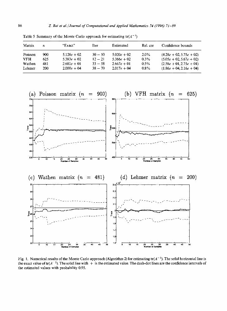
We now present numerical examples of Algorithm 2 for the Monte Carlo estimation of the quantities tr(A-1) and det(A). Tables 5 and 6 are the summary of the results for different test

86 Z Bai et al./Journal of Computational and Applied Mathematics 74 (1996) 71-89

Table 5 Summary of the Monte Carlo approach for estimating t r (A- ~)

Matrix n "Exact" Iter Estimated Rel. err Confidence bounds

Poisson 900 5.126e + 02 30 - 50 5.020e + 02 2.0% VFH 625 5.383e + 02 12 - 21 5.366e + 02 0.3% Wathen 481 2.681e + 01 33 - 58 2.667e + 01 0.5% Lehmer 200 2.000e + 04 38 - 70 2.017e + 04 0.8%

(4.28e + 02, 5.75e + 02) (5.05e + 02, 5.67e + 02) (2.58e + 01, 2.75e + 01) (1.86e + 04,2.16e + 04)

(a) Poisson matrix (n = 900 7 5 0

600 t ' - ' ~ - ~ _ , _ ~

¢~550 i

45O

I r " ' ~ - -

3 5 0

I I

Numbm of Samples

~ 5 0 1

(b) VFH matrix (n = 625)

°I , , , ~ ' , , , ,

4501 5 10 15 25 30 35 40 45 50 Nuenlo~r of Samples

(c) 30

29

28

27

2 5

24

2 3

2 2

Wathen matrix (n = 481)

10 1'5 20 2'5 30 35 40 4'5 50 NurnbQrofSam~es

(d) Lehmer matrix (n - 200) x 10 4

2.4 . . . . . .

2,2 i ~ i - . - .

2.1 I "

j ' * ~ j ~ . .~_~-~,..+..~, ~ , . ~

f 1.8

1.7

1 .6

Number of Sampl~

Fig. 1. Numerical results of the Monte Carlo approach (Algorithm 2) for estimating tr(A- z). The solid horizontal line is the exact value oftr(A- z). The solid line with + is the estimated value. The dash-dot lines are the confidence intervals of the estimated values with probability 0.95.

Z. Bai et al./Journal of Computational and Applied Mathematics 74 (1996) 71-89

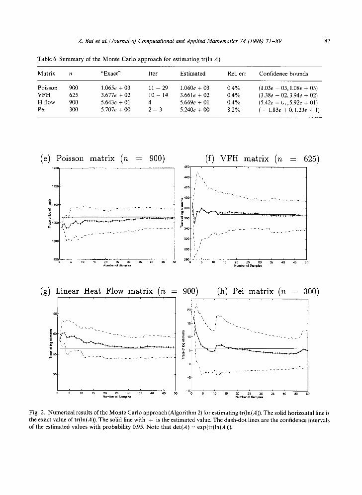
Table 6 Summary of the Monte Carlo approach for estimating tr(ln A)

87

Matrix n "Exact" Iter Estimated Re1. err Confidence bounds

Poisson 900 1.065e + 03 11 - 29 1.060e + 03 0.4% V F H 625 3.677e + 02 10 - 14 3.661e + 02 0.4% H flow 900 5.643e + 01 4 5.669e + 01 0.4% Pei 300 5.707e + 00 2 - 3 5.240e + 00 8.2%

(1.03e + 03, 1.08e + 03) (3.38e + 02, 3.94e + 02) (5.42e + t,., 5.92e + 01) ( -- 1.83e + 0, 1.23e + 1)

(e) Poisson matrix (n = 900) 1200

11oo

~ 1050

1000

950

s ~r

5 10 15 20 25 30 35 40 45 50 Number ol Samples

(f) VFH matrix (n = 625) 460,

h 440 t

/

420 J ~.

340 i ¢ _ - ...... - - - - "~ - _ _ .

320 i , . i

! / 300 }~

t i i i r 280; 5 10 15 210 25 310 35 4; 415 50

Number o1 Samples

(g) Linear Heat Flow matrix (n = 900'

.=*

6o "6

55

5 0

- - - - s . . . . . - , -

1/

5 10 15 20 25 30 35 40 45 50 Number ol Samples

(h) Pei matrix (n = 300)

0

-5

- IG

1 A 201 ~,

+ \ Z .......

Number of Samples

I I [

35 40 45 50

Fig. 2. Numerical results of the Monte Carlo approach (Algorithm 2) for estimating tr(ln(A)). The solid horizontal line is the exact value of tr(ln(A)). The solid line with + is the estimated value. The dash-dot lines are the confidence intervals of the estimated values with probability 0.95. Note that det(A) = exp(tr(ln(A))).

88 Z. Bai et aL /Journal o f Computational and Applied Mathematics 74 (1996) 71-89

matrices. Figs. 1 and 2 show the history of the Monte Carlo approach where the number of sample vectors zf is m = 50. Linear heat fl0w, VFH and Poisson test matrices have been described above. The additional three test matrices are from the Higham's test matrix collection [9]:

Wathen matrix: It is a consistent mass matrix for a regular nx x ny grid of 8-node (serendipity) elements in 2 space dimensions. The order of the matrix is n = 3nxny + 2nx + 2ny + 1. In our numerical run, we let nx = ny = 12, then n = 481 and cond(A) = 829.19.

Lehmer matrix: It is an n x n symmetric positive-definite matrix with entries afj = i/j for j /> i. The inverse of A is tridiagonal, and explicit formulas are known for its entries, n ~< cond(A) ~< 4n 2. We tested the matrix with n = 200 and cond(A) = 4.8401e + 04.

Pei matrix: A = ~I + 11 a, where 1 is an n-vector with all ones. The matrix is singular for ~ = 0, - n. We tested the matrix with n = 300, ~ = 1 and cond(A) = 301.

6. Conclusions and future work

An elegant approach for estimating the bounds of the quantity uTf(A)v has been laid out earlier in [6, 7]. The theory of matrix moments, quadrature rules, orthogonal polynomials and the underlying Lanczos procedure are beautifully connected and turned into an efficient algorithm. In this paper, we have further developed the approach in a number of practical aspects. Something old, something new, and something borrowed. Preliminary numerical results for different matrices demonstrate the high-performance of the new approach.

Our near future work includes studying the ill-conditioning problems and preconditioning techniques, improving the confidence bounds, and investigating orthogonal polynomials with variable sign [21, 5] and related quadrature rules to solve the estimation problem with u ~ v directly. The ultimate goal of this study is to develop truly efficient algorithms to solve such types of matrix computat ion problems where the matrices involved may be complex, non-Hermit ian and of order millions. These matrix computat ion problems are arising in modern lattice QCD and other scientific computing fields.

Acknowledgements

The authors would like to thank Keh-Fei Liu and Shao-Jian Dong for bringing to our attention the applications of problem (1) in the lattice QCD, and thank Shao-Jian Dong for providing the VFH test matrix. ZB and MF would also like to thank Mai Zhou for introducing them to Hoeffding's inequality used in Section 4, and to Arnold Neumaier, who reminded us of the polarization expression (3).

References

[-1] P. Davis and P. Rabinowitz, Methods of Numerical Integration (Academic Press, New York, 1984). [2] S. Dong and K. Liu, Stochastic estimation with z 2 noise, Phys. Lett. B 328 (1994) 130-136. [3] W. Gautschi, A survey of Gauss-Christoffel quadrature formulae, in: P.L. Bultzer and F. Feher, Eds., E.B.

Christoffel - the Influence of His Work on Mathematics and the Physical Sciences (Birkhauser, Boston, 1981) 73-157.

Z Bai et al./Journal of Computational and Applied Mathematics 74 (1996) 71-89 89

[4] G. Golub, Some modified matrix eigenvalue problems, SIAM Rev. 15 (1973) 318-334. [5] G. Golub and M. Gutknecht, Modified moments for indefinite weight functions, Numer. Math. 57 (1989) 607-624. [6] G. Golub and G. Meurant, Matrics, moments and quadrature, Report SCCM-93-07, Computer Science Depart-

ment, Stanford University, September 1993. [7] G. Golub and Z. Strakos, Estimates in quadratic formulas, Report SCCM-93-08, Computer Science Department,

Stanford University, September 1993. [8] G. Golub and C. Van Loan, Matrix Computations (Johns Hopkins University Press, Baltimore, MD, 2nd edn.,

1989). [9] N.J. Higham, The test matrix toolbox for Matlab, Numerical Analysis Report No. 237, University of Manchester,

England, Dec. 1993. [10] G.M. Hockney, Comparison of inversion algorithms for Wilson fermions, Nuclear Phys. B (Proc. Suppl.) 17 (1990)

301-304. [11] M. Hutchinson, A stochastic estimator of the trace of the influence matrix for laplacian smoothing splines, Commun.

Statist. Simula. 18 (1989) 1059-1076. [12] C.S. Jayanthi, S.Y. Wu and J. Cocks, The nature of vibrational modes of a self-similar fractal, Technical report,

Department of Physics, University of Louisville, KY, 1994. [13] C. Kittel, Introduction to Solid State Physics (Wiley, New York, 1972). [14] C. Lanczos, An iteration method for the solution of the eigenvalue problem of linear differential and integral

operators, J. Res. Natl. Bur. Stand. 45 (1950) 225-280. [15] A.R. Mitchell and D.F. Griffiths, The Finite Difference Method in Partial Differential Equations (Wiley, New York,

1980). [16] I. Montvay and G. Miinster, Quantum Fields on a Lattice (Cambridge Univ. Press, Cambridge 1994). [17] D. Pollard, Convergence of Stochastic Processes (Springer, New York, 1984). [18] P. Robinson and J. Wathen, Variational bounds on the entries of the inverse of a matrix, I M A J. Numer. Anal. 12

(1992) 463-486. [19] B. Sapoval, Th. Gobron and A. Margolina, Vibrations of fractal drums, Phy. Rev. Lett. 67 (1991) 2974-2977. [20] J.C. Sexton and D.H. Weingarten, The numerical estimation of the error induced by the valence approximation,

Nuclear Phys. B (Proc. Suppl.) 42 (1995) 361-363. [21] G. Struble, Orthogonal polynomials: variable-signed weight functions, Numer. Math. 5 (1963) 88-94. [22] S.Y. Wu, J.A. Cocks and C.S. Jayanthi, An accelerated inversion algorithm using the resolvent matrix method,

Comput. Phys. Commun. 71 (1992) 125-133.