Journal of Applied Geophysics 108 (2014) 69–77

Contents lists available at ScienceDirect

Journal of Applied Geophysics

j ourna l homepage: www.e lsev ie r .com/ locate / j appgeo

A concept for calculating accumulated clay thickness from boreholelithological logs and resistivity models for nitratevulnerability assessment

Anders Vest Christiansen, Nikolaj Foged ⁎, Esben AukenHydroGeophysics Group, Department of Geoscience, Aarhus University, Denmark

⁎ Corresponding author. Tel.: + 45 87162378.E-mail address: nikolaj.foged@geo.au.dk (N. Foged).

http://dx.doi.org/10.1016/j.jappgeo.2014.06.0100926-9851/© 2014 Elsevier B.V. All rights reserved.

a b s t r a c t

a r t i c l e i n f o

Article history:Received 6 September 2013Accepted 24 June 2014Available online 30 June 2014

Keywords:Nitrate vulnerabilityClay thicknessBorehole lithological logsResistivity models

We present a concept that combines lithological information from boreholes with resistivity informationfrom geophysical data to produce an accumulated clay thickness (ACT) estimate as a proxy for assessing thevulnerability of the groundwater to contamination from nitrate. The groundwater's vulnerability to nitrate isstrongly dependent on the hydraulic conductivity and the thickness of the protective layers. Low permeableclays in the overburden offer good protection to underlying aquifers by increasing the transit time. This meansthat the accumulated clay thickness is a good indicator for aquifer vulnerability to nitrate. In geophysicallyderived resistivity models clays are characterized by low electrical resistivity, but non-unique clay–sandresistivity transition prevents direct mapping of resistivity models to clay thickness. Within the ACT concept, atranslator model linking the resistivity to the accumulated clay thickness is calibrated by borehole information,ensuring consistency between the resistivity and the borehole data. An accumulated clay thickness map of theaquifer overburden (e.g., top 30m) is then calculated, based on the calibrated translatormodel and geophysicallyderived resistivity models. We demonstrate the concept on a large-scale nitrate vulnerability assessment surveyin Denmark. The concept successfully delineates the clay-dominated areas that play a key role in the assessmentof the aquifer's vulnerability to nitrate pollution.

© 2014 Elsevier B.V. All rights reserved.

1. Introduction

The vulnerability of aquifers in relation to contaminations from landuse is a key parameter in areal management (Foster, 1987) in majorparts of the world where the supply of drinking water is dependenton groundwater. This is the case in e.g. Europe where approximately70% of the water supply is based on groundwater (Navarrete et al.,2008) while e.g. in India the percentage is 85%. Contamination oftenoriginates from pesticides, fertilizers, or industry. Nitrate is mentionedspecifically in the EU Nitrate directive in which member states arerequired to take appropriate measures to ensure that agriculturalnitrate is reduced in the environment and particularly in areas identifiedas nitrate vulnerable. The vulnerability of an aquifer can be defined as itssensitivity to contamination by surface, or near-surface pollutants(Casas et al., 2008). This definition recognizes that the vulnerabilitydepends on the characteristics of the site; therefore, different soil andhydrogeological settings will result in different amounts of exposureto the aquifer.

A commonly used model to assess groundwater vulnerability tocontaminants is the DRASTIC groundwater index (Aller et al., 1987),

which has been customized and applied in a number of differentgroundwater vulnerability scenarios (Assaf and Saadeh, 2009;Baalousha, 2010; Babiker et al., 2005; Leone et al., 2009). The DRASTICindex includes hydrogeological parameters of (D) depth to watertable, (R) recharge, (A) aquifer media, (S) soil media, (T) topography,(I) impact of vadose zone and (C) conductivity (hydraulic). Each catego-ry has a rating from 0 to 10 and is assigned differentweights resemblingits relative importance in the calculation. Boreholes offer many of thekey input parameters, but often the spatial density is low and thereforethey cannot provide sufficient information to calculate large-scalevulnerability maps with the necessary detail and quality. A higherdensity can be obtained from geophysical measurements of the resis-tivity of the subsurface. Especially airborne EM methods are suitableas theymap large areas in a short time and by choosing the right systemthey also have sufficient resolution in the near surface (upper 30 m)needed for the delineation of the geological layers. Dabas et al. (2012)showed how to integrate geophysical results in an indirect way toreach an improved DRASTIC-based vulnerability map. In this case thegeophysical results were used to produce a soil map and to confirmand update the geological map of the area. This led to better and moredetailed information about the R, S, A, and C parameters in the index.

Kirsch et al. (2003) also use geophysical data, but in a purelygeophysically based vulnerability index. Their index is based on a

Fig. 1. Flow chart of ACT concept. The translator model (2) is updated until thegeophysically-derived clay thickness is consistent with the borehole clay thickness. Thisoptimum translator model (6) is then applied to the resistivity models to achieve thefinal optimum clay thickness map (7).

70 A.V. Christiansen et al. / Journal of Applied Geophysics 108 (2014) 69–77

summationwith depth of the electrical conductance (product of electri-cal conductivity and layer thickness) of the resistivity models. In thiscase the resistivity information originated from a helicopter EM survey.Casas et al. (2008) used resistivity information from ground based DCcross sections in an electrical conductance vulnerability index.

Generally, the conductivity (or resistivity) to lithology relationship isquite complex because the formation conductivity is affected by, amongother things, porosity, saturation, pore water conductivity, clay content,and clay mineral type with varying Cation Exchange Capacity (CEC).Fundamental empirical models for interpreting resistivity measure-ments in rocks are Archie's law (Archie, 1942) and the shaly-sandsmodel including the CEC by Waxman and Smits (1968). Site-specificresistivity to lithology relations can be established either based onlaboratory measurements or by correlation of the survey resistivitiesto lithological borehole logs (see Beamish, 2013; Bishop et al., 2001;Mele et al., 2014 for examples).

The geochemical properties of the soil e.g. CEC, pH, and redox condi-tions are the key parameters in general vulnerability assessment. Manygeochemical processes are strongly dependent on the hydrogeologicalconditions, since the sorption and degradation processes take place dur-ing transport from the surface to the aquifers. For nitrate in particular,the parameters that affect the vulnerability are mainly the hydraulicconductivity and the thickness of the overlying geological layers,which define the transport time. For unconsolidated sediments, the hy-draulic conductivity is strongly related to the clay content (Kalinskiet al., 1993), which to some degree can be deduced from geophysicalmethods that map the resistivity of the subsurface e.g. direct current(DC) resistivity and electromagnetic (EM) techniques. Though, innear-surface clay layers part of the transport also takes place inmacropores of higher hydraulic conductivity extending from the rootzone and sometimes down to 10 m depth or more (Jorgensen andFredericia, 1992).

In Denmark, borehole and resistivity models from DC and time-domain electromagnetic (TEM) data are the primary sources of infor-mation for the geological and hydrological models, and thereby alsofor aquifer vulnerability estimation. Here, we use the accumulatedclay thickness in the upper part of the subsurface as an indicator of ni-trate vulnerability. The clay content of a formation is strongly correlatedwith its resistivity, but borehole information is needed to establish thelocal link between resistivity and lithology, since the resistivity–litholo-gy translation is dependent on the geological environment, and there-fore varies laterally. The accumulated clay thickness (ACT) conceptpresented here combines the two major sources of information,geophysically-derived resistivity models and lithological borehole logs,in an optimization approach (in geophysics termed inversion, in hydrol-ogy termed calibration). The resistivity input for the ACT-concept needsto be spatially dense and needs to have a good near-surface resolution.For example this could be resistivity models from airborne frequencydomain systems or airborne time domain systems with a high nearsurface resolution such as the SkyTEM101 system (Schamper et al.,2014). In the field case we used resistivity models from the groundbased Pulled Array Continuous Electrical Sounding system (PACES)(Sørensen, 1996) contributing detailed information about the top 20–25 m.

The resulting spatially distributed accumulated clay thickness mapsare tailored for vulnerability assessment by combining the locallydetailed borehole information with information on the spatial hetero-geneity from the geophysics.

2. Methodology

The ACT concept estimates the accumulated clay thickness in adepth interval based on geophysical resistivity models and lithologicalinformation from boreholes. It is based on an inversion algorithm,which seeks to minimize the difference between clay thickness ob-served in boreholes and clay thickness translated from geophysics.

The inversion procedure iteratively updates the model parameters in apetrophysical model (the translator model), which converts the geo-physical resistivities to meters of clay, seeking the smallest differencebetween boreholes and geophysics.

The inversion algorithm in its basic form consists of a nonlinearforward mapping of the model to the data space:

∂Tobs ¼ G∂mtrue þ ebor ð1Þ

where δTobs denotes the difference between the observedACT (Tbor) andthe non-linear mapping of the model to the data space (Tfor). δmtrue

represents the difference between the true translator model and anarbitrary referencemodel. ebor is the observational error, and G denotesthe Jacobianmatrix that contains the partial derivatives of themapping.The general solution to the non-linear inversion problem of Eq. (1) isdescribed in Appendix A, which is based on Auken and Christiansen(2004) and Auken et al. (2005). In the following we will introducethe ACT-concept starting with an over-view followed by a detaileddescription of each component.

The flowchart in Fig. 1 gives an overview of the ACT-concept, with adetailed description following this overview. Starting from the top inthe flowchart: The resistivity models, typically from TEM and/or DCmeasurements, and the translator model form the forward response,Tfor (boxes 1, 2 and 3, Fig. 1). The observed clay thicknesses (Tbor) anduncertainties (ebor) are extracted from the lithological log of the bore-holes (boxes 4 and 5, Fig. 1). The parameters of the translator modelare updated during the inversion to obtain consistency between theTfor and the Tbor values. The output is an optimum resistivity-to-claythickness translatormodel (box 6, Fig. 1).When applying this translatormodel to the resistivity models, we then obtain the clay thickness mapfor the survey area (box 7, Fig. 1).

2.1. The translator model

In a sedimentary depositional environment it can be assumed ingeneral that low resistivities correspond to clay or clay rich sedimentsand high resistivities correspond to non-clay sediments, silt, sand,

Fig. 2. The translator model and interpolation by point kriging. a) shows the translatormodel defined by the two resistivity threshold values (mlow and mup). b) shows thetranslatormodel applied to nodepoints in a grid covering the survey area, enablinguniquedefinition of the translator model anywhere through simple interpolation. c) illustratestheuse of point kriging to interpolate the geophysical clay thickness values to the boreholelocations.

71A.V. Christiansen et al. / Journal of Applied Geophysics 108 (2014) 69–77

gravel, chalk etc. Fig. 2a shows the translator model returning a weight,W, between 0 and 1 for a given resistivity value, ρ. The translator modelis based on a scaled complementary error function (erfc) defined by alower resistivity value, mlow, and an upper resistivity value; mup. mlow

and mup represent the clay and sand cutoff values respectably so forresistivity values below mlow the layer is counted as clay (W ≈ 1) andfor resistivity values above mup the layer is counted as sand (W ≈ 0).The translator model (W(ρ)) is mathematically defined as:

W ρð Þ ¼ 0:5 � erfcK � 2ρ−mup−mlow

� �mup−mlow

� �0@

1A;

K ¼ erfc−1 0:0025 � 2ð Þð2Þ

where K scales the complementary error function so that weights of0.975 and 0.025 are returned for ρ equal to mup and mlow, respectively.Using the translatormodel in Fig. 2a, a 10m thick layer with a resistivityof e.g. 45Ωmgets aweight of 0.5 corresponding to clay thickness of 5mclay for this layer. For a layered resistivity model the clay thickness isthen calculated for theN layers and summarized to get the accumulatedclay thickness (Tfor):

Tfor ¼XN

iW ρið Þ � ti; ð3Þ

where W(ρi) is the clay weight for the resistivity in layer i and ti is thethickness of the resistivity layer included in the depth interval for theTfor calculation. Of course the geophysical resistivity model needs tohave a reasonable resolution of the subsurface resistivities in the Tfordepth interval.

To allow spatial variations in the translator model, a regular modelgrid is defined for the survey area, each node holding the two para-meters of the translator mode (Fig. 2b). A simple bilinear interpolationis used to calculate the parameters of the translator model at the posi-tions of the resistivity models shown with the white dots in Fig. 2b.

2.2. The forward response

As described in the previous section, the first step in calculating Tfor,is to apply the translator model to the resistivity models. The secondstep is to interpolate the Tfor values from the resistivity model positionsto the borehole positions (T*for) for evaluation. The interpolation isperformed by point kriging (Fig. 2c), which involves setting a search ra-dius from the estimation points (the borehole positions), and a semi-variogram function. The experimental semi-variogram is calculatedbased on all the Tfor values assuming stationarity. Normally the experi-mental semi-variogram can be approximated well with an exponentialfunction. The search radius depends on the density of the resistivitymodels and the boreholes and the model grid setup. Typically, a searchradius of up to 500 m balances the need for accurate estimations and afast calculation time of the kriging algorithm. We use the open sourcegeostatistical modeling code Gstat (Pebesma and Wesseling, 1998) forkriging, variogram calculation, and variogram fitting.

The benefits of using kriging for interpolation are that it takesthe spatial variance of the Tfor into account, and as importantly, it alsoprovides uncertainty estimates of T*for which include the original un-certainty of Tfor and the interpolation uncertainty. These uncertaintyestimates are needed for a meaningful evaluation of the data misfit atthe borehole positions.

The variance of Tfor, var(Tfor), from Eq. (3) is

var T for

� �¼ var ∑N

i¼1W ρið Þ � ti� �

: ð4Þ

This involves calculating the variance of a sum, a product and thecomplementary error-function as a function ρ. For a resistivity model,the resistivity and thickness of a layer are often correlated and theyare also correlated to the resistivities and thicknesses of the neighboringlayers in the model. To make an exact calculation of the Tfor variancefrom Eq. (4), we therefore need to know the full covariance matrix ofthe geophysical model. In some cases we have variance estimates ofresistivities and thickness, but the covariances are rarely given by thegeophysical inversion routines.

To estimate the Tfor variance we therefore make the followingassumptions:

• The Tfor variances for resistivities in layers are independent.Presumably, the resistivity variances layer to layer are negativelycorrelated (increasing the resistivity of one layer can becounterbalanced by a decrease in the next layer to produce thesame response) indicating that this assumption results in a con-servative variance estimate.

• For a given resistivity layer we neglect the variance of the thick-ness. Neglecting the variance of the thickness for a few-layeredmodel is a consequence of the first assumption, since an increasein layer thickness of one layer will subsequently lead to a decreaseof the thickness for another layer. For a multilayer resistivitymodel with fixed layer boundaries there is no variance on thethicknesses.

With the assumptions above we can make the error propagation forindependent variables (Ku, 1966) and rewrite Eq. (4) as:

var Tfor

� �¼XNi¼1

ti �∂W ρð Þ∂ρ j

ρ¼ρi

!2

var ρið Þ: ð5Þ

The derivative of the complementary error function is defined as,

∂∂z erfc zð Þ ¼ − 2ffiffiffi

πp e−z2 ð6Þ

Fig. 3. The black square marks the location of the Hadsten study area.

Fig. 4. TheHadsten area. Boreholes aremarkedwith color-coded circles specifying the claythickness in the upper 30m. Blue lines mark the positions of the PACES resistivity models.The green dots show the translator model grid.

72 A.V. Christiansen et al. / Journal of Applied Geophysics 108 (2014) 69–77

and then the weight function differentiated with respect to ρ becomes:

∂W ρð Þ∂ρ ¼ −2 � Kffiffiffi

πp

mup−mlow

� � e− K� 2ρi−mup−mlowð Þmup−mlowð Þ

� �2

: ð7Þ

Combining Eqs. (2), (5) and (7) we can then calculate approximatevariances for Tfor.

var Tfor

� �¼XNi¼1

−2 � K � tiffiffiffiπ

pmup−mlow

� � e− K � 2ρi−mup−mlowð Þmup−mlowð Þ

� �224

352

� var ρið Þ: ð8Þ

To the complete variance description of T*for we add the varianceoriginating from the kriging interpolation itself (Pebesma andWesseling, 1998).

For a typical setup of boreholes and geophysical models the variancefrom the kriging will be the dominating part of the total variance of theT*for values. Hence, the assumptions made above concerning the inde-pendency of variables are not crucial for the final inversion results aswe will also get reasonable results even if the variances of the geo-physical models are unknown.

2.3. Borehole data and uncertainties

The data part in the ACT concept is the accumulated clay thicknessobserved in the boreholes in a depth interval (Tbor) and an uncertaintyestimate of Tbor. The depth interval corresponds to the Tfor interval.The Tbor data and uncertainty estimates are relatively subjective inputsby the user based on an evaluation of the lithological description fromthe borehole and the credibility of the sample description. At a firstglance, this should be a simple task, but it has proven to be the mosttime consuming and least objective part of the concept. The lithologiesthat contribute to the Tbor need to be defined. These lithologies arethen used to get the most likely Tbor value and the uncertainty for bore-holes for the depth interval. The uncertainty involves several subjectiveassessments when evaluating the confidence in the lithological descrip-tions and borehole meta-data.

For the Danish glacial geology we often have sand, gravel and claysoverlying Tertiary deposits of clay or chalk. The clay tills in glacialsequences and the older Tertiary clays are flagged as “protective”. Sub-jective assessment based on geological knowledge is needed whendescriptions such as ‘sandy clay till’ or ‘sand with some thin clay layers’are encountered and no general rule for handling these cases can begiven. For example, for a 10 m thick unit with the description ‘sandy-clay with some thin sand layers’ one would set the Tbor value to ~7 mand reflect the inconclusive description in the uncertainty estimate.

3. The Hadsten field case

3.1. The Hadsten area

The Hadsten area is located in the in the central part of Jutland,Denmark (Fig. 3). The geological setting of the area is a typical glaciallandscape formed during the last ice age. The area is intersected by anumber of buried valley structures at different levels (some deeperthan 100m) (Jørgensen et al., 2003a,b). The valleys are cut into the un-derlying sedimentsmainly heavy paleogene clay and chalk. The in-fill ofthe valleys consists mainly of quaternary sand and gravel, which formthe aquifers. The Hadsten area is important for the groundwater supply,and consistsmainly of farmland,withHadsten as the largest town in thearea (population 8,000). The main concern for the groundwater is ni-trate leaching from farmland, but also sulfate, chloride and pesticideshave been observed close to, and, in some cases, exceeding the maxi-mum levels allowed for drinking water (Rasmussen et al., 2011). Thearea holds 23 well fields controlled by 19 waterworks, and action

plans to ensure that the sustainability of the ground water supply isunder preparation. A key parameter in the nitrate vulnerability assess-ment for the area is the ACT map. In the next sections we present dataand results from the ACT concept for the case area located south-westof the town of Hadsten (Fig. 4).

3.2. Data and model setup

In this case the subsurface resistivities aremeasured using the PulledArray Continuous Electrical Sounding system (PACES) (Sørensen,1996). The PACES system records eight different 4-pole configurationscontinuously while pulling the electrodes on the ground surface. ThePACES data were processed and inverted with 1D-models with three

Fig. 5. The colored dots show data residual (data-fit) normalizedwith the data STD. A dataresidual of one corresponds to a fit equal to the data STD.

73A.V. Christiansen et al. / Journal of Applied Geophysics 108 (2014) 69–77

layers in a laterally constrained inversion setup (Auken et al., 2005). Athree-layer model holding five adjustable model parameters (threeresistivities and two thicknesses) is the maximum number of degreesof freedom that the PACES data can support in an inversion process.The PACES system provides detailed resistivity information of theupper 20–30 m, and a good spatial resolution is achieved with a linedensity of approximately 300 m and a model spacing of 10 m alongthe lines. The PACES lines of the area are shown in blue in Fig. 4, witha coverage of approximately 600 line kilometers, equal to about60,000 resistivity models.

In Denmark all borehole information is stored in the nationaldatabase — Jupiter (Møller et al., 2009), dating back to 1926. Today,the database holds information on more than 240,000 boreholes. Eachborehole sample in the database is assigned a lithology code from theDanish standard lithology code list. In addition to the lithology code afree-text sample description is available. Using the lithology code, anestimate of the thickness of clay layers can be queried using simpleSQL-scripts. Unfortunately, no direct quality parameters or uncertaintynumbers exist for the boreholes, the lithology descriptions and the qual-ity of the samples. To identify and exclude the poorest boreholes wehave evaluated the meta-data of the boreholes, primarily examiningthe drilling method and drilling purpose. The color-coded dots inFig. 4 mark boreholes deeper than 25 m that entered the inversionscheme. The color-coding corresponds to the accumulated clay thick-ness Tbor described in the upper 30 m of the borehole. The input bore-hole data was prepared in the following way:

• Boreholes with a depth of less than 25 m were excluded.• Old seismic shotholes and geotechnical boreholes in connectionwith freeway construction were excluded due to very poorlithological descriptions. The protective clay lithologies wereidentified and their thicknesses were summarized in the depthinterval 0–30 m to obtain Tbor.

• The uncertainty of Tbor was set +/−2 m, for the boreholescovering the full 30 m depth interval. For boreholes with a drilldepth between 25 and 30 m, the uncertainty was increased withthe difference between the 30 m and the drill depth.

Some clustering and inconsistent borehole information is observedin Fig. 4, but in general, the spatial distribution of the boreholes is rela-tively uniform. The maximum interpolation distance of the Tfor values,for evaluation against the Tbor was set to 500 m. Hence, boreholesmore than 500m away from any PACES data do not influence the inver-sion results and are in reality excluded.

The translator model grid is depicted as green dots in Fig. 4. The fullmodel grid holds 31 times 33 (1023) translator models, with a nodespacing of 500 m. The regularization constraint between neighboringnodes is set to a factor of 1.7 meaning that the mup and mlow modelparameters can vary roughly 70% from one node to the next. A uniformstarting model was used with mup = 50 Ω m and mlow = 70 Ω m res-pectively. The effective number of translator models within the areacovered by PACES measurements is 660 corresponding to 1320 modelparameters. The output of the translator models outside the PACESarea is purely driven by the model constraints and the stating model,and is therefore not to be considered in the evaluation of the results.

3.3. Results and evaluation

Fig. 5 shows the data residual normalized with the data STD, whilethe mlow and mup parameters defining the optimum resistivity to claythickness translation are plotted in Fig. 6a and b respectively. Theresulting clay thickness map is shown in Fig. 7a. The major part (67%)of the boreholes is fitted within the assumed data error (green dots inFig. 5), meaning that we obtain a good consistency between the bore-hole information and the calculated clay thickness from the PACESdata. The poorly fitted boreholes, shown with red and purple dots in

Fig. 5, aremainly placedwhere theboreholes are clustered and inconsis-tent borehole information occurs.

Spatial variations of the model parameters are shown in Fig. 6. mlow

has the lowest values to the north where it ranges from 20 to 30 Ω mand higher values in the range 60–70 Ω m to the east and to the southin the area. The spatial variation of mup is larger than for mlow, withvalues ranging from 30 to 160 Ω m. Especially south-west of Hadsten,we observe highmup parameters, meaning that relatively high resistiv-ities are translated into clay tofit the Tbor. This north-south spatial differ-ence in the translator model agrees well with the geological setting. Weknow that the ice direction was primarily from the north towards thesouth and that the Paleogene clays are closer to the surface towardsthe north. The south-moving ice would bring thick clays that wouldgradually be mixed with other sediments as the ice progressed south-wards. This process will produce clays of a lower resistivity to thenorth than to the south.

The final ACTmap in Fig. 7b shows the detailed clay thickness distri-bution, ranging fromareaswith no clay in theupper 30m(yellow color)to areas with thick clay cover (dark brown color). For comparison anACT map based only on the input borehole data is shown in Fig. 7a. Bycomparing the ACT maps of Fig. 7a and b, it is clear that the resistivitydata provide crucial information to obtain a map with a high level ofdetails. An ACT map based on a fixed translation of only resistivitydata (ACT-fixed) has been compiled for comparison and to demonstratethe benefits of the spatially varying translation. The ACT-fixed map wascreated with a single and fixed threshold value of 60Ωm. Hence, resis-tivity values below 60 Ω m are translated into clay for the entire studyarea. The difference between the ACT-fixed map and the ACT-map ofour concept (Fig. 7b) is shown in Fig. 7c. Differences in clay thicknessesin Fig. 7c are observed for large areas with an up to 20 m difference inthe clay thickness value,whichhas a significant impact in a vulnerabilityestimate. It is worth noting that the 60 Ω m limit chosen for the fixedtranslation is a qualified threshold value for the Hadsten area, resulting

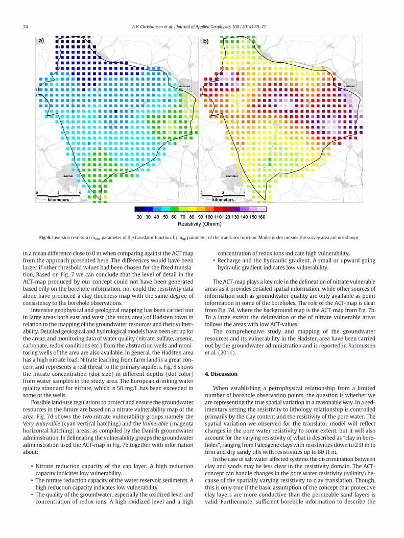
Fig. 6. Inversion results. a) mlow parameter of the translator function. b) mup parameter of the translator function. Model nodes outside the survey area are not shown.

74 A.V. Christiansen et al. / Journal of Applied Geophysics 108 (2014) 69–77

in a mean difference close to 0mwhen comparing against the ACTmapfrom the approach presented here. The differences would have beenlarger if other threshold values had been chosen for the fixed transla-tion. Based on Fig. 7 we can conclude that the level of detail in theACT-map produced by our concept could not have been generatedbased only on the borehole information, nor could the resistivity dataalone have produced a clay thickness map with the same degree ofconsistency to the borehole observations.

Intensive geophysical and geological mapping has been carried outin large areas both east and west (the study area) of Hadsten town inrelation to the mapping of the groundwater resources and their vulner-ability. Detailed geological and hydrologicalmodels have been set up forthe areas, andmonitoring data of water quality (nitrate, sulfate, arsenic,carbonate, redox conditions etc.) from the abstraction wells and moni-toring wells of the area are also available. In general, the Hadsten areahas a high nitrate load. Nitrate leaching from farm land is a great con-cern and represents a real threat to the primary aquifers. Fig. 8 showsthe nitrate concentration (dot size) in different depths (dot color)from water samples in the study area. The European drinking waterquality standard for nitrate, which is 50 mg/l, has been exceeded insome of the wells.

Possible land-use regulations to protect and ensure the groundwaterresources in the future are based on a nitrate vulnerability map of thearea. Fig. 7d shows the two nitrate vulnerability groups namely theVery vulnerable (cyan vertical hatching) and the Vulnerable (magentahorizontal hatching) areas, as compiled by the Danish groundwateradministration. In delineating the vulnerability groups the groundwateradministration used the ACT-map in Fig. 7b together with informationabout:

• Nitrate reduction capacity of the cap layer. A high reductioncapacity indicates low vulnerability.

• The nitrate reduction capacity of the water reservoir sediments. Ahigh reduction capacity indicates low vulnerability.

• The quality of the groundwater, especially the oxidized level andconcentration of redox ions. A high oxidized level and a high

concentration of redox ions indicate high vulnerability.• Recharge and the hydraulic gradient. A small or upward goinghydraulic gradient indicates low vulnerability.

The ACT-map plays a key role in the delineation of nitrate vulnerableareas as it provides detailed spatial information, while other sources ofinformation such as groundwater quality are only available as pointinformation in some of the boreholes. The role of the ACT-map is clearfrom Fig. 7d, where the background map is the ACT-map from Fig. 7b.To a large extent the delineation of the of nitrate vulnerable areasfollows the areas with low ACT-values.

The comprehensive study and mapping of the groundwaterresources and its vulnerability in the Hadsten area have been carriedout by the groundwater administration and is reported in Rasmussenet al. (2011).

4. Discussion

When establishing a petrophysical relationship from a limitednumber of borehole observation points, the question is whether weare representing the true spatial variation in a reasonable way. In a sed-imentary setting the resistivity to lithology relationship is controlledprimarily by the clay content and the resistivity of the pore water. Thespatial variation we observed for the translator model will reflectchanges in the pore water resistivity to some extent, but it will alsoaccount for the varying resistivity of what is described as “clay in bore-holes”, ranging from Paleogene clayswith resistivities down to 2Ωm tofirm and dry sandy tills with resistivities up to 80 Ω m.

In the case of salt water affected systems the discrimination betweenclay and sands may be less clear in the resistivity domain. The ACT-concept can handle changes in the pore water resistivity (salinity) be-cause of the spatially varying resistivity to clay translation. Though,this is only true if the basic assumption of the concept that protectiveclay layers are more conductive than the permeable sand layers isvalid. Furthermore, sufficient borehole information to describe the

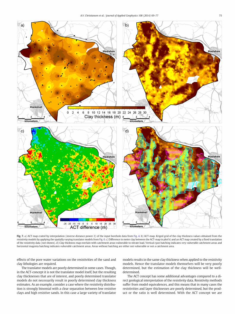
Fig. 7. a) ACT map crated by interpolation (inverse distance power 2) of the input borehole data from Fig. 4. b) ACT-map. Kriged grid of the clay thickness values obtained from theresistivitymodels by applying the spatially varying translatormodels from Fig. 6. c) Difference inmeter clay between theACT-map in plot b) and anACTmap created by a fixed translationof the resistivity data (not shown). d) Clay thickness map overlain with catchment areas vulnerable to nitrate load. Vertical cyan hatching indicates very vulnerable catchment areas andhorizontal magenta hatching indicates vulnerable catchment areas. Areas without hatching are either not vulnerable or not a catchment area.

75A.V. Christiansen et al. / Journal of Applied Geophysics 108 (2014) 69–77

effects of the pore water variations on the resistivities of the sand andclay lithologies are required.

The translator models are poorly determined in some cases. Though,in the ACT-concept it is not the translator model itself, but the resultingclay thicknesses that are of interest, and poorly determined translatormodels do not necessarily result in poorly determined clay thicknessestimates. As an example, consider a casewhere the resistivity distribu-tion is strongly binomial with a clear separation between low resistiveclays and high resistive sands. In this case a large variety of translator

models results in the same clay thicknesswhen applied to the resistivitymodels. Hence the translator models themselves will be very poorlydetermined, but the estimation of the clay thickness will be well-determined.

The ACT concept has some additional advantages compared to a di-rect geological interpretation of the resistivity data. Resistivity methodssuffer from model equivalences, and this means that in many cases theresistivities and layer thicknesses are poorly determined, but the prod-uct or the ratio is well determined. With the ACT concept we are

Fig. 8. Nitrate concentration (NO3) in different depths for the Hadsten area. The dot size indicates the concentration and the dot color specifies the depth of the observation.

76 A.V. Christiansen et al. / Journal of Applied Geophysics 108 (2014) 69–77

workingwith the product of resistivity and layer thickness (Eq. (3)) andtherefore we reduce the model equivalences in the clay thicknessoutput.

The ACT concept is strongly dependent on the quality and density ofthe boreholes and geophysical data and that an acceptable consistencybetween the borehole data and the geophysical information is possible.Large misfits might be due to a strongly heterogenetic geology or to sa-line pore water that violates the basic assumptions. Though in mostcases, poorly fitted borehole data are an indication of a low boreholequality.

A more detailed quality ranking of the borehole data could probablyprovide better uncertainty estimates for the input borehole data. Thequality ranking could include parameters like drilling method, drillingpurpose, and sample density.

Of course the lateral resolution of our final clay thickness map isstrongly dependent on the density and vertical resolution of the geo-physical results. For the clay thickness map we can only obtain thesame degree of resolution as in the resistivity dataset. In our field casewe used PACES resistivity data, but resistivity results from AirborneEM surveys with good near surface resolution e.g. the SkyTEM101

system (Schamper et al., 2014) or a frequency domain system willwork as well.

5. Conclusions

We have presented a concept that combines lithological boreholeinformation with geophysical resistivity data to achieve an objectiveaccumulated clay thickness estimate in the subsurface for nitrate vul-nerability assessment. The integration of the lithological data and theresistivity models is carried out through inversion, which determinesthe optimum translator model that describes a simple petrophysical re-lationship between resistivity and clay thickness. The basic assumptionis that low resistivities correspond to protective clays or clayey sedi-ments, and high resistivities correspond to highly permeable non-claysediments. The inversion concept allows lateral variation in the trans-lation, with smoothness constraints as regularization, and handles

uncertainties on both input and output data. The most time consumingand less objective part of the concept is the description of the clay thick-ness for the boreholes and the associated uncertainty estimates.

The ACT concept was applied to the Hadsten area for a nitratevulnerability assessment. Here the clay thickness was estimated in theupper 30 m, which provided a detailed spatial information regardingthe aquifers' vulnerability that cannot be obtained with a limited num-ber of boreholes in the area. The final clay thickness map played a keyrole in the designation of nitrate vulnerable areas. In general theHadsten area has a high nitrate load, and as a consequence to this,approximately 60% of the area was declared vulnerable to nitrate.

Acknowledgments

The research for this paper has been carried outwithin the STAIR3D-project (funded by Geo-Center Denmark) and the HyGEM-project(funded by the Danish Council for Strategic Research, DSF 11-116763).We also wish to thank the DanishMinistry of the Environment, The Na-ture Agency for granting access to data for the field case, and Assoc. Pro-fessor Emeritus Niels B. Christensen for inspiring discussion and input,Senior Researcher Verner Søndergaard, now at the Geological Surveyof Denmark and Greenland (GEUS), for inspiring us to develop the algo-rithm in the first place, senior researcher Flemming Jørgensen at GEUSfor numerous discussions on borehole descriptions and how to evaluatethe results from the ACT algorithm and head of department at GEUS,Flemming Larsen for providing us with valuable insight into nitratereduction processes in tills and clay formations.

Appendix A

The inversion scheme for the ACT-concept is almost identical to thescheme of the inversion code AarhusInv (Auken et al., accepted forpublication) and described in detail in Auken et al. (2005). To solvethe inversion problem we minimize the misfit between observed datadobs having associated errors given by eobs, and the forward responsefunction g(m).

77A.V. Christiansen et al. / Journal of Applied Geophysics 108 (2014) 69–77

In order to solve this problemwe use a first order approximation forthe non-linear function, g, mapping from model space vectors, m, intodata space:

dobs þ eobs≅G mtrue−mref

� �þ g mref

� �: ð9Þ

Here, mref is some reference model vector holding the model para-meters of the resistivity to clay translator function, mtrue is the truemodel vector, and G is the Jacobian matrix. The equation can be furtherrewritten in terms of successive iterative model updates δmtrue:

Gδmtrue ¼ δdobs þ eobs ð10Þ

where δdobs = dobs − g(mref).

The full inversion scheme also includes the regularizing constraintsbetween the model parameters in the model grid and support for apriori information. This is included adding two more sets of equations.The full system of equations can then be stated as:

GRI

24

35 ¼ δmtrue ¼

δdobsδr

δmprior

24

35þ

eobsereprior

24

35 ð11Þ

where er is the error on the constraints, with 0 as expected value. δr=−Rmref claims identity between the parameters tied by constraints inthe roughening matrix R. I is the identity matrix, δmprior is a vectoridentifying the prior model.

These equations are solved in a least squares sense by minimizingthe L2 misfit using an iterative Gauss–Newton minimization schemewith a Marquardt modification. With this approach we obtain a systemof linear equations to solve for iterative model updates:

GTC−1obsGþ RTC−1

c R þ C−1prior þ λI

� �� δm

¼ GTC−1obs dobs−g mnð Þð Þ þ RTC−1

c −Rmnð Þ þ C−1prior mprior−mn

� �: ð12Þ

Here, mn is the model vector for the n'th iterative step, and δm themodel update for the next iteration. Cobs, Cprior and Cc are diagonalcovariance matrices holding the uncertainty on the observed data,prior model and constraints, respectively. λ is a Marquart dampingparameter (Marquart, 1963). During each iteration of the inversion aline search is performed, solving the system for different values of λuntil a model update of suitable magnitude is found.

Estimation of the uncertainty for the model parameters can beobtained by the linearized covariance matrix Cest, calculated from thefollowing expression (Tarantola and Valette, 1982):

Cest ¼ GTC−1obsGþ RTC−1

c R þ C−1prior

� �−1: ð13Þ

In our case the inversion is performed in logarithmical model spaceto prevent negative model parameters.

References

Aller, L., Bennett, T., Lehr, J.H., Petty, R.J., Hackett, G., 1987. DRASTIC: a Standardized Sys-tem for Evaluating Ground Water Pollution Potential Using Hydrogeologic Settings:US EPA, 600/2-87-035.

Archie, G.E., 1942. The electrical resistivity log as an aid in determining some reservoircharacteristics. Trans. AIME 146, 54–62.

Assaf, H., Saadeh, M., 2009. Geostatistical assessment of groundwater nitrate contamina-tion with reflection on DRASTIC vulnerability assessment: the case of the upper litanibasin, Lebanon. Water Resour. Manag. 23, 775–796.

Auken, E., Christiansen, A.V., 2004. Layered and laterally constrained 2D inversion of resis-tivity data. Geophysics 69, 752–761.

Auken, E., Christiansen, A.V., Jacobsen, B.H., Foged, N., Sørensen, K.I., 2005. Piecewise 1Dlaterally constrained inversion of resistivity data. Geophys. Prospect. 53, 497–506.

Auken, E., Christiansen, A.V., Kirkegaard, C., Fiandaca, G., Schamper, C., Behroozmand, A.A.,Binley, A., Nielsen, E., Effersø, F., Christensen, N.B., Sørensen, K.I., Foged, N., Vignoli, G.,2014. An overview of a highly versatile forward and stable inverse algorithm for air-borne, ground-based and borehole electromagnetic and electric data. Explor.Geophys. (accepted for publication).

Baalousha, H., 2010. Assessment of a groundwater quality monitoring network using vul-nerability mapping and geostatistics: a case study from Heretaunga Plains, NewZealand. Agric. Water Manag. 97, 240–246.

Babiker, I.S., Mohamed, M.A.A., Hiyama, T., Kato, K., 2005. A GIS-based DRASTIC model forassessing aquifer vulnerability in Kakamigahara Heights, Gifu Prefecture, centralJapan. Sci. Total Environ. 345, 127–140.

Beamish, D., 2013. Petrophysics from the air to improve understanding of rock propertiesin the UK. First Break 31, 63–71.

Bishop, J., Sattel, J., Munday, T., 2001. Electrical structure of the regolith in the Lawlers Dis-trict, Western Australia. Explor. Geophys. 32, 20–28. http://dx.doi.org/10.1071/EG01020.

Casas, A., Himi, M., Diaz, Y., Pinto, V., Font, X., Tapias, J.C., 2008. Assessing aquifer vulner-ability to pollutants by electrical resistivity tomography (ERT) at a nitrate vulnerablezone in NE Spain. Environ. Geol. 54, 515–520.

Dabas, M., Jubeau, T., Rouiller, D., Larcher, J.M., Charriere, S., Constant, T., 2012. Using high-resolution electrical resistivity maps in a watershed vulnerability study. First Break30, 51–56.

Foster, S.S.D., 1987. Fundamental concepts in aquifer vulnerability, pollution risk and pro-tection strategy. In: van Duijvenbooden, W., van Waegeningh, H.G. (Eds.), TNO Com-mittee on Hydrological Research: the Hague, Vulnerability of Soil and Groundwaterto Pollutants. Proc Inf, 38, pp. 69–86.

Jorgensen, P.R., Fredericia, J., 1992. Migration of nutrients, pesticides and heavy metals infractured clayey till. Geotechnique 42, 67–77.

Jørgensen, F., Lykke-Andersen, H., Sandersen, P., Auken, E., Nørmark, E., 2003a. Geophys-ical investigations of buried Quaternary valleys in Denmark: an integrated applica-tion of transient electromagnetic soundings, reflection seismic surveys andexploratory drillings. J. Appl. Geophys. 53, 215–228.

Jørgensen, F., Sandersen, P., Auken, E., 2003b. Imaging buried Quaternary valleys using thetransient electromagnetic method. J. Appl. Geophys. 53, 199–213.

Kalinski, R.J., Kelly, W.E., Pesti, G., Pesti, B., 1993. Electrical resistivity measurements to es-timate travel times through unsaturated ground water protective layers. J. Appl.Geophys. 30, 161–173.

Kirsch, R., Sengpiel, K.P., Voss, W., 2003. The use of electrical conductivity mapping in thedefinition of an aquifer vulnerability index. Near Surf. Geophys. 1, 13–19.

Ku, H.H., 1966. Notes on the use of propagation of error formulas. J. Res. Natl. Bur. Stand.70C.

Leone, A., Ripa, M.N., Uricchio, V., Deák, J., Vargay, Z., 2009. Vulnerability and risk evalua-tion of agricultural nitrogen pollution for Hungary's main aquifer using DRASTIC andGLEAMS models. J. Environ. Manag. 90, 2969–2978.

Marquart, D., 1963. An algorithm for least squares estimation of nonlinear parameters.SIAM J. Appl. Math. 11, 431–441.

Mele, M., Inzoll, S., Giudici, M., Bersezio, R., 2014. Relating electrical conduction of alluvialsediments to textural properties and pore-fluid conductivity. Geophys. Prospect 62,631–645. http://dx.doi.org/10.1111/1365-2478.12102.

Møller, I., Verner, H., Søndergaard, V.H., Flemming, J., Auken, E., Christiansen, A.V., 2009.Integrated management and utilization of hydrogeophysical data on a nationalscale. Near Surf. Geophys. 7, 647–659.

Navarrete, C.M., Olmedo, J.G., Valsero, J.J.D., Gómez, J.D.G., Espinar, J.A.L., Gómez, J.A.D.L.O.,2008. Groundwater protection in Mediterranean countries after the European waterframework directive. Environ. Geol. 54, 537–549.

Pebesma, E.J., Wesseling, C.G., 1998. Gstat: a program for geostatistical Modelling, predic-tion and simulation. Comput. Geosci. 24, 17–31.

Rasmussen, S., Nyholm, T., and Nielsen, E., 2011, Afgiftsfinansieret grundvandskortlægning -Redegørelse for Hadsten-området Abbott, S., Ed., Danish Ministry of the Environment,ISBN: 978-87-92227-23-2, Danish Ministry of the Environment, ISBN: 978-87-92227-23-2.

Schamper, C., Auken, E., Sørensen, K.I., 2014. Coil response inversion for very early timemodelling of helicopter-borne time-domain electromagnetic data and mapping ofnear-surface geological layers. Geophys. Prospect. http://dx.doi.org/10.1111/1365-2478.12104.

Sørensen, K.I., 1996. Pulled array continuous electrical profiling. First Break 14, 85–90.Tarantola, A., Valette, B., 1982. Generalized nonlinear inverse problems solved using a

least squares criterion. Rev. Geophys. Space Phys. 20, 219–232.Waxman,M.H., Smits, L.J.M., 1968. Electrical conductivities in oil-bearing shaly sands. Soc.

Pet. Eng. J. 8, 107–122.