Embed Size (px)
Citation preview

SEMCOM Page 1 of 31CHARUTAR VIDYA MANDAL’S
SEMCOMVALLABH VIDYANAGER
Faculty Name: Dr. Kamlesh VaishnavClass: T.Y.B.C.A.Subject: Operation ResearchTopic: Study Material Date: 22-06-2015
UNIT – 41. Project Scheduling in PERT/CPM
2. Sequencing Problems 3. Dynamic Programming
1. Project Scheduling in PERT-CPM
Introduction
A project defines a combination of interrelated activities which must be executed in a certain order before the entire task can be completed. The activities are interrelated in a logical sequence in such a way that some activities cannot start until some others are completed. An activity in a project is usually viewed as job requiring time and resources for its completion.
Until recently, planning was seldom used in the design phase. As the technological development took place at a very rapid speed and the designs become more complex with more inter-departmental dependence and interaction, the need for planning in the development phase become inevitable.
Until five decades ago, the best known ‘planning tool’ was the so called Gantt Bar Chart (GBC) which specifies the start and finish times for each activity on a horizontal time-scale. The disadvantage of Gantt Chart (GBC) is that the interdependency between different activities (that mainly controls the progress of the project) cannot be determined from the bar chart (GBC). Growing complexities of modern projects have demanded more systematic and effective planning techniques with the objective of optimizing the efficiency of executing the project. Efficiency implies effecting the utmost reduction in the time required to complete the project while accounting for economic feasibility of using available resources. Project Management has evolved as a new field with the development of two ‘analytic’ techniques for planning, scheduling and controlling of projects. These are the Critical Path Method (CPM) and the Project Evaluation and Review Technique (PERT).

SEMCOM Page 2 of 31Historical Development of CPM / PERT Techniques
In 1956-58, above two techniques were developed by two different groups almost simultaneously. CPM was developed by Walker from E. L. du pont de Nemours Company to solve project scheduling problems and was later extended to a more advanced status by Mauchly Associates. During the same time, PERT was developed by the team of engineers working on the Polar’s Missile Programme of US Navy. This was a large project involving many departments and there were many activities about which they had a very little information about the duration of the project. Under such conditions, the project was to be completed within a specified time. To coordinate activities of various departments, this group used PERT and devised the technique independent of CPM.
The methods are essentially network-oriented techniques using the same principle. PERT and CPM are basically time-oriented methods in the sense that they both lead to the determination of a time schedule for the project. The significant difference between two approaches is that the time estimates for the different activities in CPM were assumed to be deterministic while in PERT these were described probabilistically. Now-a-days, PERT and CPM actually comprise one technique and the differences, if any are only historical. Therefore, these techniques are referred to as ‘project scheduling’ techniques, and together called PERT/CPM.
Applications of PERT / CPM Techniques
These methods have been applied to a wide variety of problems in industries and have found acceptance even in government organizations.
These include:(i) Construction of a dam or canal system in a region,(ii) Construction of a building or highway,(iii) Maintenance or overhaul of airplanes or oil refinery,(iv) Space flight,(v) Cost control of a project using PERT / COST,(vi) Designing a prototype of a machine,(vii) Development of supersonic planes.
Network Diagram Representation
In point project scheduling; the first step is to sketch an arrow diagram which shows inter-dependencies and the precedence relationship among activities (as defined

SEMCOM Page 3 of 31below) of the project. Certain basic definitions used in a network representation of a project are given below.
1. ActivityAny individual operation, which utilizes resources and has an end and a beginning, is called activity. An arrow () is commonly used to represent an activity with its head indicating the direction of progress in the project (See Figure-4). These (activities) are usually classified into following four categories:
(i) Predecessor activityActivities that must be completed immediately prior to the start of another activity are called predecessor activities.
(ii) Successor activityActivities that cannot be started until one of more of other activities are completed, but immediately succeed them are called successor activities.
(iii) Concurrent activityActivities which can be accomplished concurrently are known as concurrent activities. It may be noted that an activity can be a predecessor or successor to an event or it may be concurrent with one or more of the other activities.
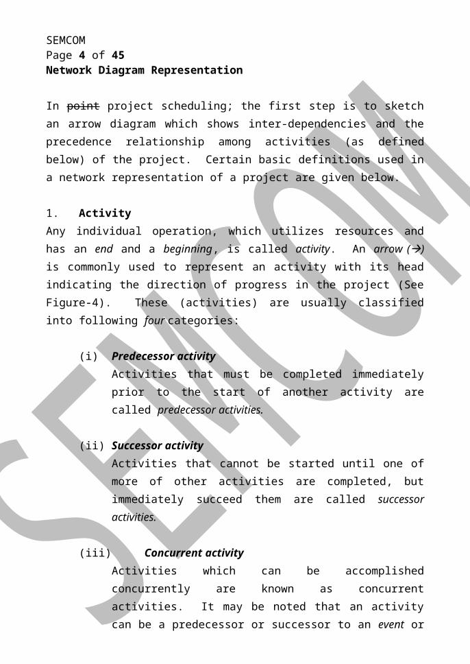
(iv) Dummy activityAn activity which does not consume any kind of resource but merely depicts the technological dependence is called a dummy activity.
It may be noted that the dummy activity is inserted in the network to clarify the activity pattern in the following two situations:
(i) to make activities with common starting and finishing points distinguishable, and
(ii) to identify and maintain the proper precedence relationship between activities that are not connected by events.
For example, consider a situation where A and B are concurrent activities, C is dependent on A, and D is dependent on A and B both. Such a situation can be handled by using a dummy activity as follows (Figure – 1).
SEMCOM Page 4 of 31
Figure – 1
In another situation, consider the following diagram where job B and C have the same job reference and they can be started independently on completion of A. But, D could be started only after completion of B and C. This relationship is shown by the dotted line (Figure – 2).
Figure – 2
2. EventAn event represents a point in time signifying the completion of some activities and the beginning of new ones. This is usually represented by a circle ‘O’ in a network which is also called a node or connector.
The events can be further classified into following three categories (as shown below in the Figure – 3).
(i) Merge eventWhen more than one activity comes and joins an event, such event is known as merge event.
(ii) Burst event
SEMCOM Page 5 of 31When more than one activity leaves an event, such event is known as a burst event.
(iii) Merge and burst eventAn activity may be a merge and burst event at the same time as with respect to some activities it can be a merge event and with respect to some other activities it may be a burst event.
Figure – 3
Figure – 4
Remarks:
1. An event is that particular instant of time at which some specific part of a project has been or is to be achieved. An activity is actual performance of a task. An activity requires time and resources for its completion.
Examples of events: design completed, pipe line laid, etc.Examples of activities: assembly of parts, mixing of concrete, preparing budget, etc.
2. Events are described by such words as: completed, started, issued, approved, tested, etc. While the words like: design, procure, test, develop, prepare etc. shows that work is being accomplished and thus represent activities.

SEMCOM Page 6 of 313. While drawing networks, it is assumed that (i) time flows from left to right,
and (ii) head events always have number higher than that of tail event. Thus activity (i – j) always means that the job which begins at event ‘i’ is completed at event ’j’. Because i is the head event and j is the tail even in the activity (ij).
4. Network representation is based on the following two axioms:(i) An event is not said to be complete until all the activities flowing into
it are completed.(ii) No subsequent activity can begin until its tail event is reached or
completed.
Rules for Drawing Network Diagram
Rules for drawing network diagrams are summarized as follows:
Rule 1 Each activity is represented by one and only one arrow in the network
This implies that no single activity can be represented twice in the network. This is to be distinguished from the case where one activity is broken into segments. In such a case, each segment may be represented by a separate arrow. For example, in laying down a pipe, this may be done in sections rather than as one job.
(a) (b)
Figure – 5

SEMCOM Page 7 of 31Rule 2 No two activities can be identified by the same end events
For example, activities a and b (Figure – 5(a)) have the same end events. The procedure is to introduce a dummy activity either between a and one of end events or between b and one of the end events. Modified representations after introducing the dummy d are shown in Figure – 5(b). As a result of using the dummy d, activities a and b can now be identified by unique end events. It must be noted that a dummy activity does not consume any time or resources.
Dummy activities are also useful in establishing logic relationship in the arrow diagram which otherwise cannot be represented correctly. Suppose jobs a and b in a certain project must precede the job c. On the other hand, the job e is preceded by the job b only. Figure – 6 (a) shows, the incorrect way since, though the relationship between a, b and c are correct, the diagram implies that the job e must be preceded by both the jobs a and b. The correct representation using the dummy activity d is shown in Figure-6 (b) that shows/justifies the indicated precedence relationships clearly.
Figure – 6
Rule 3 In order to ensure the correct precedence relationship in the arrow diagram, following questions must be checked whenever any activity is added to the network.
(i) What activity must be completed immediately before this activity can start?

SEMCOM Page 8 of 31(ii) What activities must follow this activity?(iii) What activities must occur simultaneously with this activity?
A few important suggestions for drawing good networks are given below:
Suggestions:If two or more individuals draw the same network for a given project, it seldom happens that some of them will look alike. As a matter of fact, no two of them may even look similar. The reason is that there are many ways to draw the same network. However, there will be same network representation drawn from above set of rules which are much easier to follow than the other. In the case of a large network, it is essential that certain ‘good habits’ be practiced to draw an ‘easy to follow’ network.
(1) Try to avoid arrows which cross each other.(2) Use straight arrows.(3) Do not attempt to represent duration of activity by its arrow length.(4) Use arrows from left to right (or right to left). Avoid mixing two directions.
Vertical (standing) arrows may be used if necessary.(5) Use dummies freely in rough draft but final network should not have any
redundant dummies.(6) The network has only one entry point – called the start event and one point of
emergence (coming out) – called the end event.
In many situations, all these may not be compatible with each activity and some of them are violated. The idea of having a simple network is to facilitate easy reading for all those who are involved in the project.
Common Errors in Drawing Networks
Three types of errors are most commonly observed in drawing network diagrams.
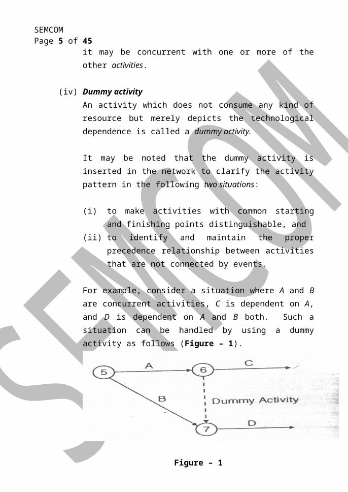
(1) DanglingTo disconnect an activity before the completion of all activities in a network diagram is known as dangling. As shown in the Figure – 7, activities (5-10) and (6-7) are not the last activities in the network. So the diagram is wrong and indicates the error of dangling.

SEMCOM Page 9 of 31
Figure – 7: Dangling Error Diagram
(2) Looping (or Cycling)Looping error is also known as cycling error in a network diagram. Drawing an endless loop in a network is known as an error of looping as shown in the following figure (Figure – 8).
Figure – 8: Looping (or Cycling) Error Diagram
(3) RedundancyUnnecessarily inserting the dummy activity in a network logic is known as the error of redundancy as shown in the following diagram (Figure – 9).

SEMCOM Page 10 of 31Figure – 9 : Redundancy Error
LABELLING: FULKERSONS’S ‘I-J’ RULE
For the network representations, it is necessary that various nodes be properly labeled. For convenience, labeling is done on the network diagram. A standard procedure, called the ‘I-J’ rule developed by D.R. Fulkerson, is most commonly used for this purpose. Main steps of this procedure are:
(a) A start event is the one which has arrows emerging from it but none entering it. Find the start event and number it as unity (1).
(b) Delete all arrows emerging from all numbered events. This will create at least one new start event out of preceding events.
(c) Number all new start events ‘2’, ‘3’, and so on (no definite rule is necessary, but numbering from ‘top to bottom’ may facilitate other users in reading the network when there are more than one new start events.
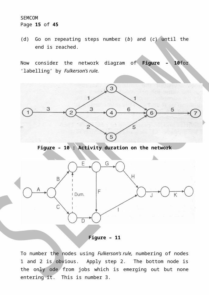
(d) Go on repeating steps number (b) and (c) until the end is reached.
Now consider the network diagram of Figure – 10for ‘labelling’ by Fulkerson’s rule.
Figure – 10 : Activity duration on the network

SEMCOM Page 11 of 31
Figure – 11
To number the nodes using Fulkerson’s rule, numbering of nodes 1 and 2 is obvious. Apply step 2. The bottom node is the only ode from jobs which is emerging out but none entering it. This is number 3.
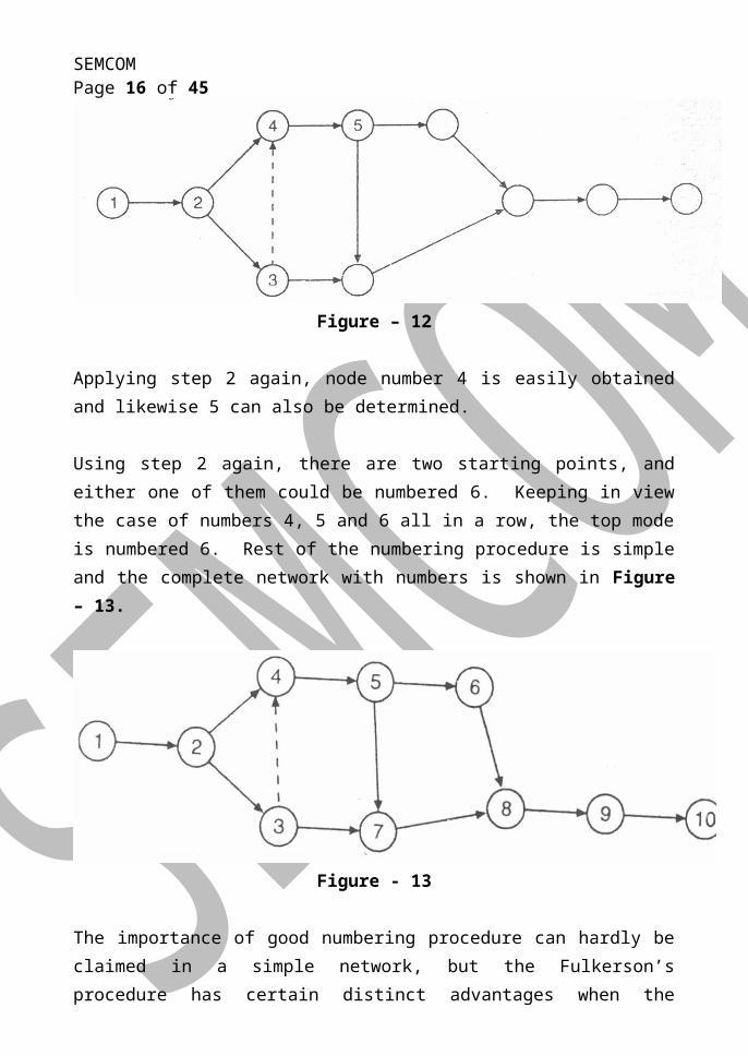
Figure – 12
Applying step 2 again, node number 4 is easily obtained and likewise 5 can also be determined.
Using step 2 again, there are two starting points, and either one of them could be numbered 6. Keeping in view the case of numbers 4, 5 and 6 all in a row, the top mode is numbered 6. Rest of the numbering procedure is simple and the complete network with numbers is shown in Figure – 13.

SEMCOM Page 12 of 31
Figure - 13
The importance of good numbering procedure can hardly be claimed in a simple network, but the Fulkerson’s procedure has certain distinct advantages when the network is large. First, the Fulkerson’s procedure will always detect a close loop in the network if there is any. In network methods, a close loop represents an impossible event. Second, numbers are smaller toward the start side and become larger on the end. A third advantage will become apparent when a matrix representation of the network is brought for computerization.
Forward Pass Computations (For Earliest Event Time)
Before starting computations, the occurrence time of initial network event is fixed. Then, the forward pass computation yields the earliest start and earliest finish time for each activity (i, j), and indirectly the earliest expected occurrence time for each event. This is mainly done in three steps.
Step 1 The computations begin from the ‘start’ node and move towards the ‘end’ node. For easiness, the forward pass computations start by assuming the earliest occurrence time of zero for the initial project event.
Step 2 (i) Earliest starting time of activity (i, j,) is the earliest event time of the tail end event i.e., (Es)ij = Ei.
(ii) Earliest finish time of activity (i, j) is the earliest starting time + the activity time i.e., (Ef)ij = (Es)ij + Dijor (Ef)ij = Ei+ Dij.
(iii) Earliest event time for event j is the maximum of the earliest finish times of all activities ending into that event. That is, Ej =
SEMCOM Page 13 of 31max
i [(Ef)ijfor all immediate predecessor of (i, j)] or Ej = max
i
[Ei + Dij]
The computed ‘E’ values are put over the respective circles representing each event.
Backward Pass Computations (For Latest Event Time)
The latest event times (L) indicates the time by which all activities entering into that event must be completed without delaying the completion of the project. These can be computed by reversing the method of calculation used for earliest event times. This is done in the following steps:
Step 1 For ending event assume E = L. Remember that all E’s have been computed by forward pass computations.
Step 2 Latest finish time for activity (i, j) is equal to the latest event time of event j, i.e., (Lf)ij = Lj.
Step 3 Latest starting time of activity (i, j) = the latest completion time of (i, j) – the activity time.
Step 4 Latest event time for event i is the minimum of the latest start time of
all activities originating from that event, i.e., Li = min
j [(Ls)ij for all
immediate successors of (i, j)] = min
j [(Lf)ij – Dij] = min
l [Lj – Dij]
The computed ‘L’ values are put over the respective circles representing each event.
Determination of Floats and Slack Times
When the network diagram is completely drawn, properly labelled, and earliest (E) and latest (L) event times are computed as discussed so far, the next object is to determine the floats and slack times defined as follows:
There are mainly following kinds of floats:
(1) Total float

SEMCOM Page 14 of 31The amount of time by which the completion of an activity could be delayed beyond the earliest expected completion time without affecting the overall project duration time.
Mathematically, the total float of an activity (i – j) is the difference between the latest start time and earliest start time of that activity. Hence the total float for an activity (i – j), denoted by (Tf)ij, can be calculated by the formula: (Tf)ij
= (Latest start – Earliest start) for activity (i – j) or (Tf)ij= (Ls)ij – (Es)ijor (Tf)ij
= (Lj – Dij) - Ei.
This is the most important type of float because of concerning with the overall project duration.
(2) Free float
The time by which the completion of an activity can be delayed beyond the earliest finish time without affecting the earliest start of a subsequent (succeeding) activity.
Mathematically, the free float for activity (i, j), denoted by (Ff)ij, can be calculated by the formula: (Ff)ij = (Ej – Ei) - Dij.
In other words, Free float for (i – j) = (Earliest time for event j – Earliest time for event i) – Activity time for (i, j).
This float is concerned with the commencement of subsequent activity.
(3) Independent Float (Short Question: What is independent float?)
The amount of time by which the start of an activity can be delayed without effecting the earliest start time of any immediately following activities, assuming that the preceding activity has finished at its latest finish time.
Mathematically, independent float of an activity (i, j) denoted by (If)ij can be calculated by the formula:
(If)ij = (Ej – Li) – Dij
The negative independent float is always taken Zero. This float is concerned with prior and subsequent activities.
It can be observed that: Independent float <= Free Float <= Total Float
SEMCOM Page 15 of 31Remarks:Floats are used to represent under-utilized resources and flexibility of the schedule.Note that whenever a float in a particular activity is utilized, the float of other activities would also change.
Remarks
1. We know that (Tf)ij = (Lj – Ei) – Dij. But, Lj>Ej as latest event time is always greater than or equal to the earliest event time. Therefore, (Tf)ij> (Ej – Ei) – Dij or (Tf)ij> (Ff)ij. Hence for all activities, free float can take values from zero up to total float, but it cannot exceed total float.
2. Free float is very useful for rescheduling the activities with minimum disruption of earlier plans.
Determination of Critical Path
Before defining critical path, let us first discuss about the meaning of critical event and critical activity.
Critical Event
Since the slack of an event is the difference between the latest and earliest event times, i.e., slack(i) = Li – Ei, the events with zero slack times are called critical events.
In other words, the event (i) is said to be critical if Ei = Li.
Critical activity
Since the difference between the latest start time and earliest start time of an activity is usually called as total float, the activities with zero total float are known as critical activities.
In other words, an activity is said to be critical if a delay in its start will cause a further delay in the completion date of the entire project.
SEMCOM Page 16 of 31Obviously, a non – critical activity is such that the time between its earliest start and its latest completion dates (as allowed by the project) is longer than its actual duration. In this case, non-critical activity is said to have a slack or float time.
Critical Path
The sequence of critical activities in a network is called the critical path.
The critical path is the longest path in the network from the starting event to ending event and defines the minimum time required to complete the project.
By the term ‘path’ we mean a sequence of activities such that it begins at the starting event and end at the final event. The length of a path is the sum of the individual times of the activities lying on the path.
If the activities on critical path are delayed by a day, the project would also be delayed by a day unless the times of the future critical activities are reduced by a day by different means. The critical path is denoted by double or darker lines to make distinction from the other non-critical paths.
Main features of critical path
The critical path has two main features:
(i) If the project has to be shortened, then some of the activities on that path must also be shortened. The application of additional resources on other activities will not give the desired result unless that critical path is shortened first.
(ii) The variation in actual performance from the expected activity duration time will be completely reflected in one-to-one fashion in the anticipated completion of the whole project.
The critical path identifies all critical activities of the project. The method of determining such a path is explained by the following numerical example.
Example 1.Consider the following network where nodes have been numbered according to the Fulkerson’s rule. Numbers along various activities represent the normal time (Dij) required to finish that activity, e.g. activity (3) – (6) will take 5 days (months, weeks, hours depending on the time units). For this project, we are

SEMCOM Page 17 of 31interested to find out the time it will take to complete this project. What jobs are critical to the completion of the project in time, etc?
Figure - 14
Solution. For this, it is necessary to find out the earliest and the latest completion time for each activity in the network. The earliest and the latest times are re-calculated by using ‘forward pass’ and ‘backward pass’ computations, respectively.
To understand the procedure, we define:
Ei= the earliest expected occurrence time of event i,Lj= the latest allowable event occurrence time for event j. This is the latest time by
which the event j must be started without increasing the project duration.Dij= the expected duration to complete the activity i–j.
The solution now starts by the forward pass computation.
Step 1 Determination of Earliest Time (Ej): Forward Pass ComputationThe purpose of the forward pass computation is to find out earliest start times for all the activities. For this, it is necessary to assign some initial value to the starting node 1. Usually this value is taken to be zero so that the subsequent earliest time could be interpreted as the project duration up to that point in question.
Rules for the computation are as follows:
Rule 1 Initial event is supposed to occur at time equal to zero, that is, E1= 0.

SEMCOM Page 18 of 31
Rule 2 Any activity can start immediately when all preceding activities are
completed. The earliest time Ej for node j is given by Ej= max
i [Ei + Dij], where i is the collection of nodes which precede node j.
Rule 3 Repeat step 2for the next eligible activity until the end node is reached.
Numerical Calculation:
Consider the network (Figure - 14) by assumption E1 = 0 and E2 = max
i [Ei + Di2].
For node 2, node 1 is the only predecessor and hence i = 1 contains only one element. Therefore, E2 = E1 + D12 = 0 + 2 = 2.
Likewise, values of E3, E4, E5, and E6can be computed as:E3 = E1 + D13 = 0 + 2 = 2, E4 = E1 + D14 = 0 + 2 = 2, E5 = E2 + D25 = 2 + 4 = 6, E6 = E3
+ D36 = 2 + 5 = 7.
Consider node 7, where there are three emerging entering activities, i.e., E7 = max
i (Ei
+ Di7),
The collection i consists of nodes 3, 4 and 6 that are preceding node 7. Therefore,
E7 = max [E3 + D37 = 2 + 8 = 10, E4 + D47 = 2 + 4 = 6,E6 + D67 = 7 + 0 = 7] = 10E8 = max [E5 + D58 = 6 + 2 = 8, E6 + D68 = 7 + 4 = 11] = 11E9 = max [E8 + D89 = 11 + 3 = 14, E7 + D79 = 10 + 5 = 15*] = 15 and E10 = E9 + D9,10 = 15 + 4 = 19.
From this computation, it can be inferred that this job will take 19 days to finish as this is the longest path of the network. Activities along this longest path are: 1 – 3, 3 – 7, 7 – 9 and 9 – 10. This longest path is called the critical path. In any network, it is not possible that there can be only one critical path. For example, if in the above network let D36 = 6 days, then two critical paths exist having the same duration for completion of project.
Step 2 Determination of Latest Time (Li): Backward Pass ComputationIn forward pass computation, the earliest time when a particular activity will be completed is known. It is also seen that some activities

SEMCOM Page 19 of 31are not critical to the completion of the job. The question, a manager would like to ask is: Can their starting time be delayed so that the total completion time is still the same? Such a question may arise while scheduling the resources such as: manpower, equipment, finance and so on. If delay is allowable, then what can be the maximum delay? For, this is the latest time for various activities which is desired. The backward pass computation procedure is used to calculate the latest time the latest time for various activities. In the forward pass computation, assignment E1 = 0 was arbitrary, likewise for the backward pass computation, it is possible to assign the project terminal event date on which the project should be over. If no such date is prescribed, then the convention is of setting latest allowable time determined in forward pass computation.
Rule 1 Set Li = Ei or Ts where Ts is the scheduled date for completion and Ei is the earliest terminal time.
Rule 2 Li = min
j {Lj – Dij}, i.e. the latest time for activities is the minimum of the latest time of all succeeding activities reducing their activity time.
Rule 3 Repeat rule 2until staring activity is reached.
Latest times for activities of the network are calculated below:
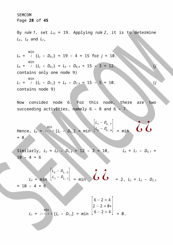
By rule 1, set L10 = 19. Applying rule 2, it is to determine L9, L8 and L7,
L9 = min
j {Lj – D9, j} = 19 – 4 = 15 for j = 10.
L8 = min
j {Lj – D8, j} = L9 – D8, 9 = 15 – 3 = 12. (j contains only one node 9)
L7 = min
j {Lj – D7, j} = L9 – D7, 9 = 15 – 5 = 10. (j contains node 9)
Now consider node 6. For this node, there are two succeeding activities, namely 6 – 8 and 6 – 7.
Hence, L6 = min
j = (7 , 8 )[Lj – D6, j] = min [L7 − D6 , 7
L8 − D6, 8 ] = min ¿¿ = 8.
SEMCOM Page 20 of 31Similarly, L5 = L8 – D5, 8 = 12 – 2 = 10, L4 = L7 – D4, 7 = 10 – 4 = 6
L3 = min [L6 − D3 , 6
L7 − D3 , 7 ] = min ¿¿ = 2, L2 = L5 – D2, 5 = 10 – 4 = 6
L1 = min
j = (2 , 3 , 4 )[Lj – D1, j] = min [ 6 − 2 = 42 − 2 = 0∗6 − 2 = 4 ]
= 0.
Figure - 15
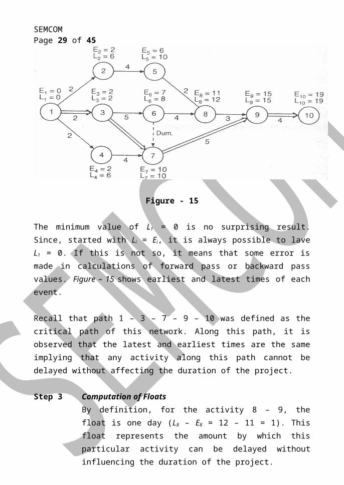
The minimum value of L1 = 0 is no surprising result. Since, started with Li = Ei, it is always possible to lave L1 = 0. If this is not so, it means that some error is made in calculations of forward pass or backward pass values. Figure – 15 shows earliest and latest times of each event.
Recall that path 1 – 3 – 7 – 9 – 10 was defined as the critical path of this network. Along this path, it is observed that the latest and earliest times are the same implying that any activity along this path cannot be delayed without affecting the duration of the project.
Step 3 Computation of FloatsBy definition, for the activity 8 – 9, the float is one day (L8 – E8 = 12 – 11 = 1). This float represents the amount by which this particular activity can be delayed without influencing the duration of the project.

SEMCOM Page 21 of 31
Also, by definition, free float, if any, will exist only on the activities merge points. To illustrate the concept of free float, consider path 1 – 2 – 5 – 8 – 9, total float on activity 8 – 9 is one day and since this is the last activity prior to merging two activities, this float is free float also. Similarly, consider the activity 5 – 8 which has a total float of 4 days but has only 3 days of free float because 1 day of free float is due to the activity 8 – 9. If the activity 5 – 8 s delayed up to three days, the early start time of no activity in the network will be affected. Therefore, the concept of free float clearly states that the use of free float time will not influence any succeeding activity float time.
If free float of any activity comes out to be negative, it is taken zero. For example, independent float of (1, 2) = free float of (1, 2) – (L1 – E1) = 0 – (0 – 0) = 0.
Step 4 To identify Critical PathThe earlier calculation shows that the path or paths which have zero float are called the critical ones. If this logic is extended little further, it would provide a guide rule to determine the next most critical path, and so on. Such an information will be useful for managers in the control of projects. In this example, path 1 – 3 – 8 – 9 – 10 happens to be next to critical path; because it has float of one day on many of its activities.
Activity(i– j)
Duration(Dij)
Earliest Latest FloatStart Finish Start Finish
Total Free
(1) (2) (3)(4)= (3) + (2)
(5)=(6)- (2)
(6)
1 – 21 – 31 – 42 – 53 – 63 – 74 – 75 – 8
22245842
00022226
222671068
404632610
626108101012
40441044
00000043
SEMCOM Page 22 of 316 – 87 – 98 – 99 – 10
4534
7101115
11151419
8101215
12151519
1010
0010
Activity(i – j)
Duration(Dij)
Start Finish Float
EarliestEi LatestLiEarliest
EjLatestLj Total Free
(1) (2) (3) (4)(5)
= (3) + (2)
(6)= (4) + (2)
(7)= (4) –
(3)
(8) = Ej –
Ei of
successive
activity
1 – 21 – 31 – 42 – 53 – 63 – 74 – 75 – 86 – 87 – 98 – 99 – 10
222458424534
000222267101115
4046326108101215
22267106811151419
62610810101212151519
404410441010
000000430010
The method discussed earlier is easily adoptable on computers. In the case of small networks, we can perform most of the calculations right on the diagram. In an event that a person would like to use tableau format to find floats, etc, such methods are also available. Table above summarizes float times and other information.

SEMCOM Page 23 of 312. JOB SEQUENCING
Definition of Job Sequencing
Suppose there are n jobs (1, 2, . . ., n), each of which has to be processed one at a time at each of m machines A, B, C , . . . The order of processing each job through machines is given. The time that each job must require on each machine is known. The problem is to find a sequence among (n !¿¿m number of all possible sequences for processing the jobs so that the total elapsed time for all jobs will be minimum.
Mathematically, letAi = time for job i on machine A,Bi = time for job i on machine B,T = time from start of first job to completion of the last job.
Then, the problem is to determine for each machine a sequence of jobsi1 , i2 ,i3 ,. . . ,in ,where (i1 ,i2 ,i3 , .. . ,in) the permutation of the integers which will minimize T.
PROCESSING n JOBS THROUGH TWO MACHINES
The problem can be described as: (i) only two machines A and B are involved (ii) each job is processed in the order AB, and (iii) the exact or expected processing time A1 , A2 , A3 , . .. , An , ;B1 , B2,B3 , . . . , Bnare known.
Processing times Job (i)1 2 3 .. .. n
Ai A1 A2 A3 .. .. An
Bi B1 B2 B3 .. .. Bn
Problem is to sequence (order) the jobs so as to minimize the total elapsed time T.The solution procedure adopted by Johnson (1954) is given below.
JOHNSON’S ALGORITHM FOR nJOBS 2 MACHINES
Then Johnson’s iterative procedure for the determining the optimal sequence for an n-job 2-machine sequencing problem can be outlined as follows.
Step1. Examine the Ai ' s and Bi ' s for i=1 , 2 ,. . . ,n¿ and find out mini
[ Ai ,B i].Step2. (i) If this minimum be Ak for somei=k, do (process) the k th job first of
all. (as the given order is AB)(ii) If this minimum be Br for somei=r , do (process) the rth job last of
all. (as the given order is AB)
Step3. (i) If there is a tie for minimum Ak=B r, process the k th job first of all and r th job in the last.

SEMCOM Page 24 of 31(ii) If the tie for minimum occurs among the Ai ' s, select the job
corresponding to the minimum of Bi ' s and process it first of all.(iii) If the tie for minimum occurs among theBi ' s, select the job
corresponding to the minimum of Ai ' s and process it in the last. Go to next step.
Step4. Cross out the jobs already assigned and repeat steps 1 to 3 arranging the jobs next to first of next to last, until all the jobs have been assigned.
The resulting ordering will minimize the elapsed time T.
Example
Consider the five jobs 1, 2, 3, 4, and 5 needs to be processed on two machines A and B in the order AB. The time for processing each job on both the machines are give below.
Processing Time (in Hours)Job 1 2 3 4 5Time for A 5 1 9 3 10Time for B 2 6 7 8 4
Determine a sequence for five jobs that will minimize the elapsed time T. Calculate the total idle time for the machines in this period.
Solution
Step-1: Mini [Ai, Bi] = 1 for A2. So, place A2 job first:
2
Step-4: Remaining Jobs are:1 3 4 55 9 3 102 7 8 4
Step-1: Mini [Ai, Bi] = 2 for B1. So, place B2 job last:
2 1
Step-4: Remaining Jobs are:3 4 59 3 107 8 4
Step-1: Mini [Ai, Bi] = 3 for A4. So, place A4 job at first empty position that is after A2:
2 4 1

SEMCOM Page 25 of 31Step-4: Remaining Jobs are:
3 59 107 4
Step-1: Mini [Ai, Bi] = 4 for B5. So, place B5 job previous to last:2 4 5 1
Thus the final sequence of jobs are2 4 3 5 1
Minimum elapsed time corresponding to the optimal sequencing 2-4-3-5-1
Machine – A Machine – BJob Sequence Time In Time Out Time In Time Out
2 0 1 1 74 1 4 7 153 4 13 15 225 13 23 23 271 23 28 28 30
The idle time for machine – A: 28-30 (2 Hours)The idle time for machine – B: 0-1, 22-23, 27-28 (3 Hours).Hence, the Total elapsed time is 5 Hours.
Examples
In a machine shop 8 different products are being manufactured each requiring time on two different machines A and B are given in the table below:
Product 1 2 3 4 5 6 7 8Machine-A 30 45 15 20 80 120 65 10Machine-B 20 30 50 35 35 40 50 20
Find an optimal sequence of processing of different product in order to minimize the total manufactured time for all product. Find total ideal time for two machines and elapsed time.
In a machine shop 6 different products are being manufactured each requiring time on two different machines A and B are given in the table below:
Product 1 2 3 4 5 6Machine-A 30 120 50 20 90 110Machine-B 80 100 90 60 30 80
Find an optimal sequence of processing of different product in order to minimize the total manufactured time for all product. Find total ideal time for two machines and elapsed time.
In a printing shop 7 different books are printed and bounded on two different machines A and B. Time required on two machines are given in the table below:
Product 1 2 3 4 5 6 7Printing 3 4 8 3 6 7 5

SEMCOM Page 26 of 31Binding 8 6 3 7 2 8 4
Find an optimal sequence of processing of different product in order to minimize the total manufactured time for all product. Find total ideal time for two machines and elapsed time.
Assumptions in Sequencing ProblemShort Question: Write down any two assumptions used for solving sequencing problem.
Answer (Write down any two)1. No machine can process more than one operation at a time.2. Each operation, once started, must be performed till completion.3. A job is an entity, i.e. even though the job represents a lot of individual parts,
no lot may be processed by more than one machine at a time.4. Each operation must be completed before any other operation, which it much
precede, can begin.5. Time intervals for processing are independent of the order in which operations
are performed.6. These is only one of each type of machine.7. A job is processed as soon as possible subject to ordering requirements.8. All jobs are known and are ready to start processing before the period under
consideration begins.9. The time required to transfer jobs between machines is negligible.

SEMCOM Page 27 of 313. DYNAMIC PROGRAMMING
Introduction
Dynamic programming is a mathematical technique dealing with the optimization of multistage decision process. The word ‘programming’ has been used in the mathematical sense of selecting an optimum allocation of resources, and it is ‘dynamic’ as it is particularly useful for problems where decisions are taken at several distinct stages, such as every day or every week.
Richard Bellman developed this technique in early 1950 and invented its name. Dynamic programming can be given a more significant name as recursive optimization.
In dynamic programming, a large problem is split into small sub-problems each of them involving only a few variables. This technique converts one problem of n variables into n sub-problems (stages), each in one variable.
The optimum solution is obtained in an orderly manner starting from one stage to the next, and is completed till the final stage is reached.
To convert a verbal problem into a multistage structure is not always simple, and sometimes it becomes very difficult and even looks easy to apply. Recursion equations are of standard nature and its computer program runs in a standard routine.
An important point is that – the problem of successive stages be treated separately even though by the very nature of the problem these stages are dependent? The answer of this question is based on ‘Bellman’s Principle of Optimality’ which is stated in the following section.
Discrete and continuous, deterministic as well as probabilistic models can be solved by this method. Thus dynamic programming method is very useful for solving various problems, such as inventory, replacement, allocation, linear programming, etc. A single constraint problem is relatively simple, but in the problem of more than two constraints more complexities appear.
(i) While solving the problem we use the concepts of stage and state. Moreover, the problem is solved stage by stage and to ensure that suboptimal solution does not result, we cumulated the objective function value in a particular way. Working backwards, for every stage, we found the decisions in that
SEMCOM Page 28 of 31stage that will allow us to reach the final destination optimally, starting from each of the states of the stage. These decisions could be taken optimally, without the knowledge of how we actually reach the different states. This has been stated as the “principle of optimality in dynamic programming literature.”
(ii) State: The variable that links up two stages is called a state variable. At any stage, the status of the problem can be described by the values the state variable can take. These values are referred to as states.
(iii) Stage: The points at which decisions called for are referred to as stages. Each stage can be thought of having a beginning and an end. The different stages come in a sequence, with the ending of a stage marking the beginning of the immediately succeeding stage.
BELLMAN’S PRINCIPLE OF OPTIMALITY
Ideally, if an optimal solution is obtained for a system, any portion of it must be optimal. This is called the “Bellman’s Principle of Optimality” on which the concept of dynamic programming is based.
Short Question: State the “Bellman’s Principle of Optimality”
Answer: An optimal policy (set of decisions) has the property that whatever the initial state and decisions are, the remaining decisions must constitute an optimal policy with regard to the state resulting from the first decision.
Explanation: "...suppose that the fastest route from Los Angeles to Boston passes through Chicago. The principle of optimality translates to the obvious fact that the Chicago to Boston portion of the route is also the fastest route for a trip that starts from Chicago and ends in Boston."
In my humble formulation: If you have found an optimal policy that takes you from A to C by visiting B, you cannot find a policy for going from B to C that is better than the B to C portion of your original A-B-C policy.
The problem which does not satisfy the principle of optimality cannot be solved by the dynamic programming method.
Question: Shortest route problem
SEMCOM Page 29 of 31Answer: Given a road network and a starting node S, we want to determine the shortest path to all the other nodes in the network (or to a specified destination node). See Figure below.
This is a variation of Shortest Path Problem in Graph Theory.
In graph theory, the shortest path problem is the problem of finding a path between two vertices (or nodes) in a graph such that the sum of the weights of its constituent edges is minimized. Note that the graph can be directed. The weights on the links/arcs are costs.
Figure: Shortest path (A, C, E, D, F) between vertices A and F in the weighted directed graph
The problem is also sometimes called the single-pair shortest path problem, to distinguish it from the following variations:
The single-source shortest path problem, in which we have to find shortest paths from a source vertex v to all other vertices in the graph.
The single-destination shortest path problem, in which we have to find shortest paths from all vertices in the directed graph to a single destination vertex v. This can be reduced to the single-source shortest path problem by reversing the arcs in the directed graph.
The all-pairs shortest path problem, in which we have to find shortest paths between every pair of vertices v, v' in the graph.
These generalizations have significantly more efficient algorithms than the simplistic approach of running a single-pair shortest path algorithm on all relevant pairs of vertices.

SEMCOM Page 30 of 31Some of the most important algorithms for solving this problem are:
Dijkstra's algorithm solves the single-source shortest path problem.
Bellman–Ford algorithm solves the single-source problem if edge weights may be negative.
A* search algorithm solves for single pair shortest path using heuristics to try to speed up the search.
Floyd–Warshall algorithm solves all pairs shortest paths.
Johnson's algorithm solves all pairs shortest paths, and may be faster than Floyd–Warshall on sparse graphs.
Viterbi algorithm solves the shortest stochastic path problem with an additional probabilistic weight on each node.
Q: Introduction to Traveling Salesman Problem
A: The Travelling Salesman Problem (TSP) is an NP-hard (Non-deterministic Polynomial-time hard) problem in combinatorial optimization studied in operations research and theoretical computer science.
Given a list of cities and their pairwise distances, the task is to find the shortest possible route that visits each city exactly once and returns to the origin city.
The problem can simply be stated as: if a traveling salesman wishes to visit exactly once each of a list of m cities (where the cost of traveling from city i to city j is cij ) and then return to the home city, what is the least costly route the traveling salesman can take?
The problem was first formulated as a mathematical problem in 1930 and is one of the most intensively studied problems in optimization. It is used as a benchmark for many optimization methods.
In the traveling salesman problem we wish to find a tour of all nodes in a weighted graph so that the total weight is minimized. The traveling salesman problem is NP-hard but has many real world applications so a good solution would be useful.
The idea of the traveling salesman problem (TSP) is to find a tour of a given number of cities, visiting each city exactly once and returning to the starting city where the length of this tour is minimized.
The standard or symmetric traveling salesman problem can be stated mathematically as follows: Given a weighted graph G = (V, E) where the weight cij on the edge between nodes i and j is a non-negative value, find the tour of all nodes that has the minimum total cost. Currently the only known method guaranteed to optimally solve the traveling salesman problem of any size, is by enumerating each possible tour and

SEMCOM Page 31 of 31searching for the tour with smallest cost. Each possible tour is a permutation of 123 . . . n, where n is the number of cities, so therefore the number of tours is n!. When n gets large, it becomes impossible to find the cost of every tour in polynomial time. Many different methods of optimization have been used to try to solve the TSP.
Applications of the TSP Scheduling Jobs on Machines Controlling satellites, telescopes, microscopes, lasers...(Vehicle Routing) Computing DNA Sequences Designing Telecommunications Networks Designing and testing VLSI circuits (Computer Wiring) X-Ray Crystallography Clustering Data Arrays
The Influence of the TSP Operational Research Discrete Mathematics Theoretical Computer Science Artificial Intelligence
DisclaimerThe study material is prepared by subject teacher 2015-2016. The basic objective of this material is to supplement teaching and discussion in the classroom in the subject. Students are required to go for extra reading in the subject through library work.