Embed Size (px)
Citation preview

Josifovic, Aleksandar and Corney, Jonathan (2017) Development of
industrial process characterisation through data analysis. In: 2016 IEEE
Symposium Series on Computational Intelligence, SSCI 2016. IEEE,
Piscataway, N.J.. ISBN 978-1-5090-4241-8 ,
http://dx.doi.org/10.1109/SSCI.2016.7849990
This version is available at https://strathprints.strath.ac.uk/61597/
Strathprints is designed to allow users to access the research output of the University of
Strathclyde. Unless otherwise explicitly stated on the manuscript, Copyright © and Moral Rights
for the papers on this site are retained by the individual authors and/or other copyright owners.
Please check the manuscript for details of any other licences that may have been applied. You
may not engage in further distribution of the material for any profitmaking activities or any
commercial gain. You may freely distribute both the url (https://strathprints.strath.ac.uk/) and the
content of this paper for research or private study, educational, or not-for-profit purposes without
prior permission or charge.
Any correspondence concerning this service should be sent to the Strathprints administrator:
The Strathprints institutional repository (https://strathprints.strath.ac.uk) is a digital archive of University of Strathclyde research
outputs. It has been developed to disseminate open access research outputs, expose data about those outputs, and enable the
management and persistent access to Strathclyde's intellectual output.
Development of industrial process characterisation
through data analysis
Aleksandar Josifovic
Design, Manufacture and
Engineering Management
University of Strathclyde
75 Montrose street, Glasgow, G1 1XJ
Email: [email protected]
Jonathan Corney
Design, Manufacture and
Engineering Management
University of Strathclyde
75 Montrose street, Glasgow, G1 1XJ
Email: [email protected]
Abstract—Recently the world has seen an explosion of availabledata, gathered from sensors, experiments and direct measure-ments. The engineering world is shifting from model-centredsimulations to the exploitation of large datasets for insights intomachine behaviour. In the case of optimisation, where usually asimulation model is provided for the exploration of the parameterspace, the new data-driven approach translates into the use ofdata for quantifying problems and delivering an optimal solution.
This paper presents a methodology developed for interpreta-tion of condition monitoring data in the design process and sitecharacterisation of hydraulic fracturing. Field data samples wereprocessed to construct a nominal operating regime in a processpumping system.
After describing the generic process a case study implementa-tion of field data from a North American hydraulic fracturingsite is presented for illustration. The paper summarises sensorinstallation, data acquisition and cloud-based pre-processing.Consequent analysis demonstrates expected operational outputin normal operating conditions for a specified geological terrain.The paper concludes with a base-case scenario for PD pump’sprocess output.
I. INTRODUCTION
In recent years modern engineering systems have witnessed
the start of a shift in the process of product development from
in-depth physical modelling to increasing exploitation of real-
time monitoring of on-site operation. Machine learning, de-
veloped from Artificial Intelligence, aims to provide solutions
for problems based on developed algorithms and analysis of
historical data.
The concept of machine learning has been previously used
in many different industries and scientific studies such as
agriculture [1], mineral extraction [2], optical recognition
[3], robotics [4] and others. In industrial environment, two
approaches prevail; data collection on site and processing in
cloud or, both data collection and processing is done directly
on site.
Hydraulic fracturing process was established in 1950s [5]
and involves using large number of positive displacement (PD)
pumps to pressurise and deliver slurry-water mix into a well
[6]. This method for stimulation and increase of hydrocarbon
recovery has had global economic impact in energy sector, as
demonstrated in North America [7], [8], [9].
In this well stimulation techniques all the central processes
are controlled manually with limited amount of feedback
information related to equipment life and failure prediction.
Data processing of site metrics is currently being recorded
on site and evaluated at central locations. Initial assessment
stage needs to consider present on-site practices to develop
benchmark criteria for future exploration wells. Proposed ini-
tiative considers using characterized process metrics to develop
performance envelops for satisfactory equipment operation.
With the expansion of gathered data potential for predictive
maintenance will be feasible. This paper evaluates mechanisms
for extending equipment’s operational availability by introduc-
ing a methodology for a PD pump monitoring system.
Aim of this work is to establish methodology for develop-
ment of data processing system for hydraulic fracturing.
Systematic approach for implementing machine learning
system involves using previously recorded field metrics to char-
acterise, evaluate amplitudes and assign operational envelopes
with specific phases of the process. Specific milestones in this
work include following:
• Sensor identification and installation on equipment at
process location
• Data acquisition using specialised industrial hardware
• Upload to cloud-based system and access through be-
spoke data software
• Data evaluation using MatLab for identified process
phases
• Establishing performance envelops based on previously
examined data
II. METHODOLOGY
In Figure 1 knowledge discovery diagram is presented.
Source data - For data processing and analysis of hydraulic
fracturing processes a case study was required. Selected data
was recorded in Texas, U.S. in 2015, the upcoming sections
will present additional well properties.
Target data - Pumping stages in hydraulic fracturing typ-
ically last between 60 and 180 minutes. In addition to time
constraint two other determinants that define individual loca-
tion are required flow rates and treating pressures [10]. Case
study identifies a single pumping stage.
Data mining
Data evaluation/interpretation
Source data
Target data
Pre-processed data
Transformed data
Data patterns
Knowledge
Figure 1. Data mining and knowledge discovery diagram
Pre-processed data - Processing site information requires
selection of relevant operational metrics to be recorded for
analysis. In this case, PD pump’s inlet/outlet pressure, speed
and vibration are measured.
Transformed data - Acquired pump metrics are transformed
for display into SI units, pressure in MPa, speed in RPM and
vibration in g.
Data patterns - Physical measurements are aligned and
displayed in the same phases of pumping process. Data char-
acterisation in form of mean, extreme and frequency values
are presented for all sensor measurements.
Knowledge - Cumulative sensor output provides necessary
knowledge for site characterisation in hydraulic fracturing by
defining surface pump pressure and associated vibration for a
given pump speed.
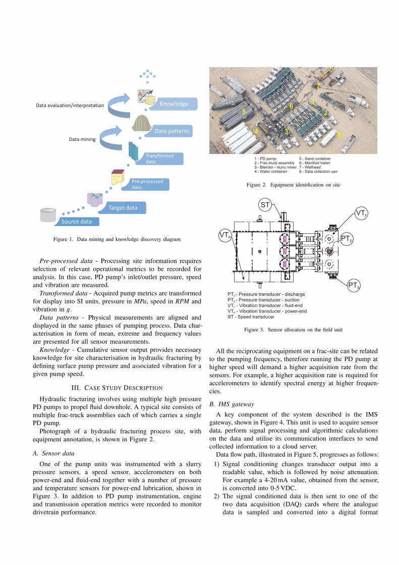
III. CASE STUDY DESCRIPTION
Hydraulic fracturing involves using multiple high pressure
PD pumps to propel fluid downhole. A typical site consists of
multiple frac-truck assemblies each of which carries a single
PD pump.
Photograph of a hydraulic fracturing process site, with
equipment annotation, is shown in Figure 2.
A. Sensor data
One of the pump units was instrumented with a slurry
pressure sensors, a speed sensor, accelerometers on both
power-end and fluid-end together with a number of pressure
and temperature sensors for power-end lubrication, shown in
Figure 3. In addition to PD pump instrumentation, engine
and transmission operation metrics were recorded to monitor
drivetrain performance.
2
1
3
5
4
6
7
1 - PD pump2 - Frac-truck assembly3 - Blender - slurry mixer4 - Water container
5 - Sand container6 - Manifold trailer7 - Wellhead8 - Data collection van
8
Figure 2. Equipment identification on site
PTD
VTF
ST
VTP
PTS
PT - Pressure transducer - discharge
PT - Pressure transducer - suction
VT - Vibration transducer - fluid-end
VT - Vibration transducer - power-end
ST - Speed transducer
D
S
F
P
Figure 3. Sensor allocation on the field unit
All the reciprocating equipment on a frac-site can be related
to the pumping frequency, therefore running the PD pump at
higher speed will demand a higher acquisition rate from the
sensors. For example, a higher acquisition rate is required for
accelerometers to identify spectral energy at higher frequen-
cies.
B. IMS gateway
A key component of the system described is the IMS
gateway, shown in Figure 4. This unit is used to acquire sensor
data, perform signal processing and algorithmic calculations
on the data and utilise its communication interfaces to send
collected information to a cloud server.
Data flow path, illustrated in Figure 5, progresses as follows:
1) Signal conditioning changes transducer output into a
readable value, which is followed by noise attenuation.
For example a 4-20mA value, obtained from the sensor,
is converted into 0-5VDC.
2) The signal conditioned data is then sent to one of the
two data acquisition (DAQ) cards where the analogue
data is sampled and converted into a digital format
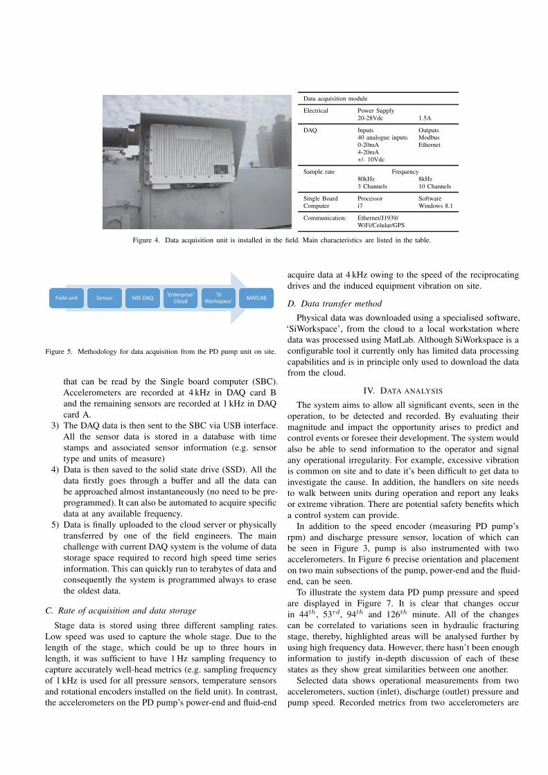
Data acquisition module
Electrical Power Supply
20-28Vdc 1.5A
DAQ Inputs Outputs
40 analogue inputs Modbus
0-20mA Ethernet
4-20mA
+/- 10Vdc
Sample rate Frequency
80kHz 8kHz
3 Channels 10 Channels
Single Board Processor Software
Computer i7 Windows 8.1
Communication: Ethernet/J1939/
WiFi/Celular/GPS
Figure 4. Data acquisition unit is installed in the field. Main characteristics are listed in the table.
Field unit Sensor IMS DAQ'Enterprise'
Cloud'SI
Workspace'MATLAB
Figure 5. Methodology for data acquisition from the PD pump unit on site.
that can be read by the Single board computer (SBC).
Accelerometers are recorded at 4 kHz in DAQ card B
and the remaining sensors are recorded at 1 kHz in DAQ
card A.
3) The DAQ data is then sent to the SBC via USB interface.
All the sensor data is stored in a database with time
stamps and associated sensor information (e.g. sensor
type and units of measure)
4) Data is then saved to the solid state drive (SSD). All the
data firstly goes through a buffer and all the data can
be approached almost instantaneously (no need to be pre-
programmed). It can also be automated to acquire specific
data at any available frequency.
5) Data is finally uploaded to the cloud server or physically
transferred by one of the field engineers. The main
challenge with current DAQ system is the volume of data
storage space required to record high speed time series
information. This can quickly run to terabytes of data and
consequently the system is programmed always to erase
the oldest data.
C. Rate of acquisition and data storage
Stage data is stored using three different sampling rates.
Low speed was used to capture the whole stage. Due to the
length of the stage, which could be up to three hours in
length, it was sufficient to have 1Hz sampling frequency to
capture accurately well-head metrics (e.g. sampling frequency
of 1 kHz is used for all pressure sensors, temperature sensors
and rotational encoders installed on the field unit). In contrast,
the accelerometers on the PD pump’s power-end and fluid-end
acquire data at 4 kHz owing to the speed of the reciprocating
drives and the induced equipment vibration on site.
D. Data transfer method
Physical data was downloaded using a specialised software,
‘SiWorkspace’, from the cloud to a local workstation where
data was processed using MatLab. Although SiWorkspace is a
configurable tool it currently only has limited data processing
capabilities and is in principle only used to download the data
from the cloud.
IV. DATA ANALYSIS
The system aims to allow all significant events, seen in the
operation, to be detected and recorded. By evaluating their
magnitude and impact the opportunity arises to predict and
control events or foresee their development. The system would
also be able to send information to the operator and signal
any operational irregularity. For example, excessive vibration
is common on site and to date it’s been difficult to get data to
investigate the cause. In addition, the handlers on site needs
to walk between units during operation and report any leaks
or extreme vibration. There are potential safety benefits which
a control system can provide.
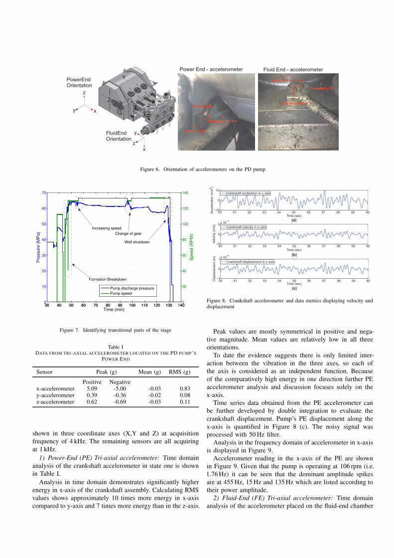
In addition to the speed encoder (measuring PD pump’s
rpm) and discharge pressure sensor, location of which can
be seen in Figure 3, pump is also instrumented with two
accelerometers. In Figure 6 precise orientation and placement
on two main subsections of the pump, power-end and the fluid-
end, can be seen.
To illustrate the system data PD pump pressure and speed
are displayed in Figure 7. It is clear that changes occur
in 44th, 53rd, 94th and 126th minute. All of the changes
can be correlated to variations seen in hydraulic fracturing
stage, thereby, highlighted areas will be analysed further by
using high frequency data. However, there hasn’t been enough
information to justify in-depth discussion of each of these
states as they show great similarities between one another.
Selected data shows operational measurements from two
accelerometers, suction (inlet), discharge (outlet) pressure and
pump speed. Recorded metrics from two accelerometers are
xy
z
PowerEndOrientation
FluidEndOrientation
x
y
z
Fluid End - accelerometerPower End - accelerometer
Figure 6. Orientation of accelerometers on the PD pump
30 40 50 60 70 80 90 100 110 120 130 1400
10
20
30
40
50
60
70
Pre
ssure
(M
Pa)
30 40 50 60 70 80 90 100 110 120 130 1400
20
40
60
80
100
120
140
Time (min)
Speed (
RP
M)
Pump discharge pressure
Pump speed
Formation Breakdown
Increasing speed
Change of gear
Well shutdown
Figure 7. Identifying transitional parts of the stage
Table IDATA FROM TRI-AXIAL ACCELEROMETER LOCATED ON THE PD PUMP’S
POWER END
Sensor Peak (g) Mean (g) RMS (g)
Positive Negativex-accelerometer 5.09 -5.00 -0.03 0.83y-accelerometer 0.39 -0.36 -0.02 0.08z-accelerometer 0.62 -0.69 -0.03 0.11
shown in three coordinate axes (X,Y and Z) at acquisition
frequency of 4 kHz. The remaining sensors are all acquiring
at 1 kHz.
1) Power-End (PE) Tri-axial accelerometer: Time domain
analysis of the crankshaft accelerometer in state one is shown
in Table I.
Analysis in time domain demonstrates significantly higher
energy in x-axis of the crankshaft assembly. Calculating RMS
values shows approximately 10 times more energy in x-axis
compared to y-axis and 7 times more energy than in the z-axis.
50 51 52 53 54 55 56 57 58 59 60−10
0
10
Time (sec)
Acce
lera
tio
n (
m/s
2
50 51 52 53 54 55 56 57 58 59 60−5
0
5x 10
−3
Time (sec)
Ve
locity (
m/s
)
50 51 52 53 54 55 56 57 58 59 60−1
0
1x 10
−6
Time (sec)
Dis
pla
ce
me
nt
(m)
Crankshaft accleration in x−axis
Crankshaft velocity in x−axis
Crankshaft displacement in x−axis
(a)
(b)
(c)
Figure 8. Crankshaft accelerometer and data metrics displaying velocity anddisplacement
Peak values are mostly symmetrical in positive and nega-
tive magnitude. Mean values are relatively low in all three
orientations.
To date the evidence suggests there is only limited inter-
action between the vibration in the three axes, so each of
the axis is considered as an independent function. Because
of the comparatively high energy in one direction further PE
accelerometer analysis and discussion focuses solely on the
x-axis.
Time series data obtained from the PE accelerometer can
be further developed by double integration to evaluate the
crankshaft displacement. Pump’s PE displacement along the
x-axis is quantified in Figure 8 (c). The noisy signal was
processed with 50Hz filter.
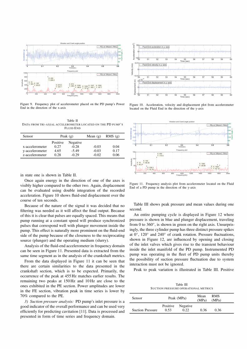
Analysis in the frequency domain of accelerometer in x-axis
is displayed in Figure 9.
Accelerometer reading in the x-axis of the PE are shown
in Figure 9. Given that the pump is operating at 106 rpm (i.e.
1.76Hz) it can be seen that the dominant amplitude spikes
are at 455Hz, 15Hz and 135Hz which are listed according to
their power amplitude.
2) Fluid-End (FE) Tri-axial accelerometer: Time domain
analysis of the accelerometer placed on the fluid-end chamber
0 0.1 0.2 0.3 0.4 0.5 0.6−4
−2
0
2
4
Time(sec)
Acceleration (g)
Vibration and Crank angle position
0 0.1 0.2 0.3 0.4 0.5 0.60
60
120
180
240
300
360
Crank Angle (
°)
PEx at 106rpm(1.76Hz)
0 200 400 600 800 1000 1200 1400 1600 1800 20000
200
400
600
800
1000
X: 15Y: 364.2
Frequency plot
Frequency(Hz)
X: 135Y: 303.5
X: 455Y: 806.4
X: 618.3Y: 224.1
Amplitude
X: 910Y: 266.7X: 1038
Y: 196.9X: 1200Y: 157.4
X: 1337Y: 195.7
X: 1500Y: 197.7
PEx at 106rpm(1.76Hz)
Figure 9. Frequency plot of accelerometer placed on the PD pump’s PowerEnd in the direction of the x-axis
Table IIDATA FROM TRI-AXIAL ACCELEROMETER LOCATED ON THE PD PUMP’S
FLUID END
Sensor Peak (g) Mean (g) RMS (g)
Positive Negativex-accelerometer 0.27 -0.28 -0.03 0.04y-accelerometer 4.65 -5.49 -0.03 0.17z-accelerometer 0.28 -0.29 -0.02 0.06
in state one is shown in Table II.
Once again energy in the direction of one of the axes is
visibly higher compared to the other two. Again, displacement
can be evaluated using double integration of the recorded
acceleration. Figure 10 shows fluid-end displacement over the
course of ten seconds.
Because of the nature of the signal it was decided that no
filtering was needed as it will affect the final output. Because
of this it is clear that pulses are equally spaced. This means that
pump running at a constant speed will produce synchronized
pulses that correspond well with plunger movement inside the
pump. This effect is naturally more prominent on the fluid-end
side of the pump because of the closeness to the reciprocating
source (plunger) and the operating medium (slurry).
Analysis of the fluid-end accelerometer in frequency domain
can be seen in Figure 11. Presented data is extracted from the
same time segment as in the analysis of the crankshaft metrics.
From the data displayed in Figure 11 it can be seen that
there are certain similarities to the data presented in the
crankshaft section, which is to be expected. Primarily, the
occurrence of the peak at 455Hz matches earlier results. The
remaining two peaks at 150Hz and 10Hz are close to the
ones exhibited in the PE section. Power amplitudes are lower
in the FE section, vibration peak in time series is lower by
70% compared to the PE.
3) Suction pressure analysis: PD pump’s inlet pressure is a
good indicator of the overall performance and can be used very
efficiently for predicting cavitation [11]. Data is processed and
presented in form of time series and frequency domain.
50 51 52 53 54 55 56 57 58 59 60−50
0
50
Time (sec)
Acceleration (m/s2)
Fluid End accleration in y−axis
50 51 52 53 54 55 56 57 58 59 60−0.01
0
0.01
Time (sec)
Velocity (m/s)
Fluid End velocity in y−axis
50 51 52 53 54 55 56 57 58 59 60−2
0
2x 10
−6
Time (sec)
Displacement (m)
Fluid End displacement in y−axis
Figure 10. Acceleration, velocity and displacement plot from accelerometerlocated on the Fluid End in the direction of the y-axis
0 0.1 0.2 0.3 0.4 0.5 0.6−1.8
−1.2
−0.6
0
0.6
1.2
1.8
Time(sec)
Acceleration (g)
Vibration and Crank angle position
0 0.1 0.2 0.3 0.4 0.5 0.60
60
120
180
240
300
360
Crank Angle (
°)
FEy at 106rpm(1.76Hz)
0 200 400 600 800 1000 1200 1400 1600 1800 20000
50
100
150
X: 10Y: 45.2
Frequency plot
Frequency(Hz)
Amplitude
X: 150Y: 58.35
X: 455Y: 110.5
X: 238.3Y: 45.76
X: 1772Y: 55.12
X: 1820Y: 52.12
X: 1363Y: 36.89
FEy at 106rpm(1.76Hz)
Figure 11. Frequency analysis plot from accelerometer located on the FluidEnd of a PD pump in the direction of the y-axis
Table III shows peak pressure and mean values during one
second.
An entire pumping cycle is displayed in Figure 12 where
pressure is shown in blue and plunger displacement, traveling
from 0 to 360◦, is shown in green on the right axis. Unsurpris-
ingly, the three cylinder pump has three distinct pressure spikes
at 0◦, 120◦ and 240◦ of crank rotation. Pressure fluctuations,
shown in Figure 12, are influenced by opening and closing
of the inlet valves which gives rise to the transient behaviour
inside the inlet manifold of the PD pump. Instrumented PD
pump was operating in the fleet of PD pump units thereby
the possibility of suction pressure fluctuation due to system
interaction must not be ignored.
Peak to peak variation is illustrated in Table III. Positive
Table IIISUCTION PRESSURE OPERATIONAL METRICS
Sensor Peak (MPa)Mean(MPa)
RMS(MPa)
Positive NegativeSuction Pressure 0.53 0.22 0.36 0.36
40 40.1 40.2 40.3 40.4 40.5 40.6 40.7 40.8 40.9 410.25
0.3
0.35
0.4
0.45
0.5
0.55
X: 40.6Y: 0.4045
Inlet Pressure
Pre
ssu
re (
MP
a)
X: 40.54Y: 0.3241
X: 40.28Y: 0.3854
X: 40.33Y: 0.3309
X: 40.1Y: 0.369
X: 40.41Y: 0.4086
X: 40.22Y: 0.4222X: 40.03
Y: 0.4113
40 40.1 40.2 40.3 40.4 40.5 40.6 40.7 40.8 40.9 410
60
120
180
240
300
360
Cra
nk A
ng
le (
°)
Cylinder no.1 Cylinder no.3
Cylinder no.2
Figure 12. Suction pressure on the inlet side of the pump during one pumpingstroke
0 0.1 0.2 0.3 0.4 0.5 0.6−0.2
0
0.2
X: 0.3554Y: −0.02484
Time(sec)
Pressure−mean(Pressure)
Inlet pressure and Crank angle position
X: 0.09983Y: −0.0003123
X: 0.2216Y: 0.06372
0 0.1 0.2 0.3 0.4 0.5 0.60
60
120
180
240
300
360
Crank Angle (
°)
Inlet pressure at 106rpm(1.76Hz)
0 10 20 30 40 50 60 70 80 90 1000
5
10
15
X: 16.67Y: 4.516
Frequency plot
Frequency(Hz)
Amplitude
X: 10Y: 6.576
X: 5Y: 13.27
Inlet frequency at 106rpm(1.76Hz)
Figure 13. Frequency spectrum of the suction pressure on the inlet side ofthe pump during one pumping stroke
pressure peak is approximately 46% higher than the mean
value. Pressure variation in the negative pressure peak is 60%.
It can be seen that peaks accurately align with the crank
angle position and the annotations in Figure 12 indicate precise
timing of the individual cylinders during one pumping cycle.
In Figure 13 a single pumping cycle is analysed in frequency
domain. The regular pressure pattern is visible in the frequency
plot. Results show regular energy spikes at 5Hz, 10Hz and
16.7Hz.
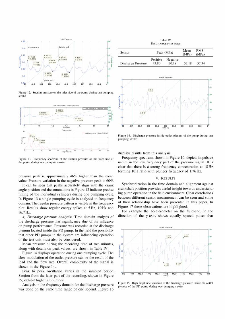
4) Discharge pressure analysis: Time domain analysis of
the discharge pressure has significance due of its influence
on pump performance. Pressure was recorded at the discharge
plenum located inside the PD pump. In the field the possibility
that other PD pumps in the system are influencing operation
of the test unit must also be considered.
Mean pressure during the recording time of two minutes,
along with details on peak values, are shown in Table IV.
Figure 14 displays operation during one pumping cycle. The
slow modulation of the outlet pressure can be the result of the
load and the flow rate. Overall complexity of the signal is
shown in the Figure 14.
Peak to peak oscillation varies in the sampled period.
Section from the later part of the recording, shown in Figure
15, exhibit higher amplitudes.
Analysis in the frequency domain for the discharge pressure
was done on the same time range of one second. Figure 16
Table IVDISCHARGE PRESSURE
Sensor Peak (MPa)Mean(MPa)
RMS(MPa)
Positive NegativeDischarge Pressure 43.80 70.18 57.18 57.34
80 80.1 80.2 80.3 80.4 80.5 80.6 80.7 80.8 80.9 8145
50
55
60
65
70
75
X: 80.26Y: 54.11
Outlet Pressure
Pre
ssure
(M
Pa)
Time (s)
X: 80.29Y: 66.53
80 80.1 80.2 80.3 80.4 80.5 80.6 80.7 80.8 80.9 810
60
120
180
240
300
360
Figure 14. Discharge pressure inside outlet plenum of the pump during onepumping stroke
displays results from this analysis.
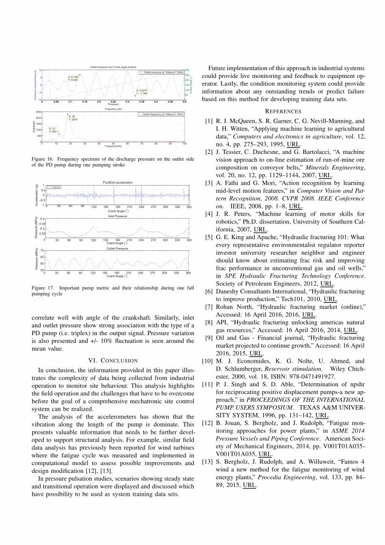
Frequency spectrum, shown in Figure 16, depicts impulsive
nature in the low frequency part of the pressure signal. It is
clear that there is a strong frequency concentration at 18Hz
forming 10:1 ratio with plunger frequency of 1.76Hz.
V. RESULTS
Synchronization in the time domain and alignment against
crankshaft position provides useful insight towards understand-
ing pump operation in the field environment. Clear correlations
between different sensor measurement can be seen and some
of their relationship have been presented in this paper. In
Figure 17 these observations are highlighted.
For example the accelerometer on the fluid-end, in the
direction of the y-axis, shows equally spaced pulses that
110 110.1 110.2 110.3 110.4 110.5 110.6 110.7 110.8 110.9 11145
50
55
60
65
70
75
X: 110.5Y: 51.82
Outlet Pressure
Pre
ssure
(M
Pa)
Time (s)
X: 110.5Y: 68.66
X: 110.7Y: 52.2
X: 110.7Y: 69.31
110 110.1 110.2 110.3 110.4 110.5 110.6 110.7 110.8 110.9 1110
60
120
180
240
300
360
Figure 15. High amplitude variation of the discharge pressure inside the outletplenum of the PD pump during one pumping stroke
0 0.05 0.1 0.15 0.2 0.25 0.3 0.35 0.4 0.45 0.5−10
−5
0
5
10
X: 0.1327Y: 6.934
Time(sec)
Pressure−mean(Pressure)
Outlet pressure and Crank angle position
X: 0.3273Y: −7.344
0 0.05 0.1 0.15 0.2 0.25 0.3 0.35 0.4 0.45 0.50
60
120
180
240
300
360
Crank Angle (
°)
Outlet pressure at 106rpm(1.76Hz)
0 10 20 30 40 50 60 70 80 90 1000
500
1000
1500
2000
2500
X: 18Y: 2310
Frequency plot
Frequency(Hz)
Amplitude
X: 12Y: 642.1
Outlet frequency at 106rpm(1.76Hz)
Figure 16. Frequency spectrum of the discharge pressure on the outlet sideof the PD pump during one pumping stroke
0 30 60 90 120 150 180 210 240 270 300 330 360-1
-0.5
0
0.5
1FluidEnd acceleration
Crank Angle (°)
Y-direction
0 30 60 90 120 150 180 210 240 270 300 330 360
0.35
0.4
0.45
0.5Inlet Pressure
Pre
ssu
re (
MP
a)
0 30 60 90 120 150 180 210 240 270 300 330 36055
60
65
70Outlet Pressure
Pre
ssu
re (
MP
a)
Crank Angle (°)
Crank Angle (°)
Acce
lera
tio
n (
g)
Figure 17. Important pump metric and their relationship during one fullpumping cycle
correlate well with angle of the crankshaft. Similarly, inlet
and outlet pressure show strong association with the type of a
PD pump (i.e. triplex) in the output signal. Pressure variation
is also presented and +/- 10% fluctuation is seen around the
mean value.
VI. CONCLUSION
In conclusion, the information provided in this paper illus-
trates the complexity of data being collected from industrial
operation to monitor site behaviour. This analysis highlights
the field operation and the challenges that have to be overcome
before the goal of a comprehensive mechatronic site control
system can be realized.
The analysis of the accelerometers has shown that the
vibration along the length of the pump is dominate. This
presents valuable information that needs to be further devel-
oped to support structural analysis. For example, similar field
data analysis has previously been reported for wind turbines
where the fatigue cycle was measured and implemented in
computational model to assess possible improvements and
design modification [12], [13].
In pressure pulsation studies, scenarios showing steady state
and transitional operation were displayed and discussed which
have possibility to be used as system training data sets.
Future implementation of this approach in industrial systems
could provide live monitoring and feedback to equipment op-
erator. Lastly, the condition monitoring system could provide
information about any outstanding trends or predict failure
based on this method for developing training data sets.
REFERENCES
[1] R. J. McQueen, S. R. Garner, C. G. Nevill-Manning, and
I. H. Witten, “Applying machine learning to agricultural
data,” Computers and electronics in agriculture, vol. 12,
no. 4, pp. 275–293, 1995, URL.
[2] J. Tessier, C. Duchesne, and G. Bartolacci, “A machine
vision approach to on-line estimation of run-of-mine ore
composition on conveyor belts,” Minerals Engineering,
vol. 20, no. 12, pp. 1129–1144, 2007, URL.
[3] A. Fathi and G. Mori, “Action recognition by learning
mid-level motion features,” in Computer Vision and Pat-
tern Recognition, 2008. CVPR 2008. IEEE Conference
on. IEEE, 2008, pp. 1–8, URL.
[4] J. R. Peters, “Machine learning of motor skills for
robotics,” Ph.D. dissertation, University of Southern Cal-
ifornia, 2007, URL.
[5] G. E. King and Apache, “Hydraulic fracturing 101: What
every representative environmentalist regulator reporter
investor university researcher neighbor and engineer
should know about estimating frac risk and improving
frac performance in unconventional gas and oil wells,”
in SPE Hydraulic Fracturing Technology Conference.
Society of Petroleum Engineers, 2012, URL.
[6] Daneshy Consultants International, “Hydraulic fracturing
to improve production,” Tech101, 2010, URL.
[7] Rohan North, “Hydraulic fracturing market (online),”
Accessed: 16 April 2016, 2016, URL.
[8] API, “Hydraulic fracturing unlocking americas natural
gas resources,” Accessed: 16 April 2016, 2014, URL.
[9] Oil and Gas - Financial journal, “Hydraulic fracturing
market projected to continue growth,” Accessed: 16 April
2016, 2015, URL.
[10] M. J. Economides, K. G. Nolte, U. Ahmed, and
D. Schlumberger, Reservoir stimulation. Wiley Chich-
ester, 2000, vol. 18, ISBN: 978-0471491927.
[11] P. J. Singh and S. D. Able, “Determination of npshr
for reciprocating positive displacement pumps-a new ap-
proach,” in PROCEEDINGS OF THE INTERNATIONAL
PUMP USERS SYMPOSIUM. TEXAS A&M UNIVER-
SITY SYSTEM, 1996, pp. 131–142, URL.
[12] B. Jouan, S. Bergholz, and J. Rudolph, “Fatigue mon-
itoring approaches for power plants,” in ASME 2014
Pressure Vessels and Piping Conference. American Soci-
ety of Mechanical Engineers, 2014, pp. V001T01A035–
V001T01A035, URL.
[13] S. Bergholz, J. Rudolph, and A. Willuweit, “Famos 4
wind a new method for the fatigue monitoring of wind
energy plants,” Procedia Engineering, vol. 133, pp. 84–
89, 2015, URL.