0/22

Lottery Equilibrium

Joshua Mollner E. Glen WeylKellogg School of Management Microsoft Research

Columbia Market Design Conference

April 13, 2018

1/22

Introduction

I Indivisibilities and non-convex preferences often presentproblems:

I general equilibrium theoryI market design

I Goal: develop a unified and simple approach to theseproblems

2/22

IntroductionGeneral equilibrium theory

I With indivisibilities and/or non-convex preferences:I competitive equilibria may fail to existI competitive equilibria may be inefficient (in a sense)

I Simple solution:I allow traders to engage in (binary) lotteriesI “lottery equilibrium”

3/22

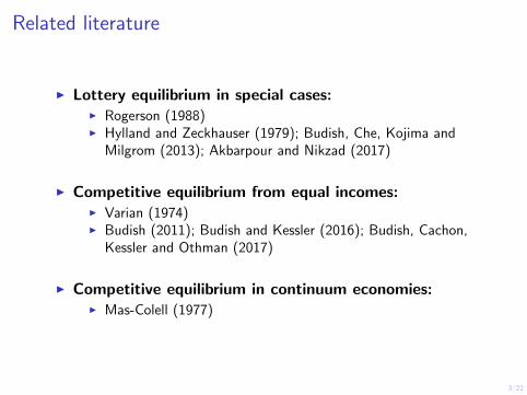
Related literature

I Lottery equilibrium in special cases:I Rogerson (1988)I Hylland and Zeckhauser (1979); Budish, Che, Kojima and

Milgrom (2013); Akbarpour and Nikzad (2017)

I Competitive equilibrium from equal incomes:I Varian (1974)I Budish (2011); Budish and Kessler (2016); Budish, Cachon,

Kessler and Othman (2017)

I Competitive equilibrium in continuum economies:I Mas-Colell (1977)

4/22

Outline

Example

Model (Continuum Economy)

ResultsExistenceFirst Welfare TheoremSecond Welfare Theorem

Next StepsFinite EconomyMarket Design Applications

5/22

ExampleEnvironment

I Consumption set: Ω = Z≥0 × [0,∞)× [0,∞)I one indivisible good “houses”I one divisible good “corn”I one divisible “artificial currency”

I Binary lotteries: ∆(Ω)

I Agents: t ∈ T = [0, 1]I utility function ut(at) = 3(1 + t)1(a1

t ≥ 1) + a2t

I endowment ωt ∈ Ω∫ωt︸ ︷︷ ︸

“inside”endowment

+

∫ψt︸ ︷︷ ︸

“outside”endowment

=

(1

2, 1, 1

)

6/22

ExampleCompetitive equilibrium vs. lottery equilibrium

Endowments (for now):

I no outside endowments:∫ψt = (0, 0, 0)

I inside endowments: ωt ∈ (1, 0, 1), (0, 2, 1)

Competitive equilibrium allocation:

I agents consume their endowments

I Pareto dominated (by a lottery allocation)

6/22

ExampleCompetitive equilibrium vs. lottery equilibrium

Endowments (for now):

I no outside endowments:∫ψt = (0, 0, 0)

I inside endowments: ωt ∈ (1, 0, 1), (0, 2, 1)

Lottery equilibrium allocation:

I t ≤ 1

3: at =

(0, 4, 1) if ωt = (1, 0, 1)

(0, 2, 1) if ωt = (0, 2, 1)

I t >1

3: at =

(1, 0, 1) if ωt = (1, 0, 1)12 · (1, 0, 1) + 0 · (0, 0, 1) if ωt = (0, 2, 1)

I Pareto efficient

7/22

Binary lotteries sufficet = 1, p = ( 4

5, 1

5, 0)

w

vt(p,w)

p · ωt = 25

7/22

Binary lotteries sufficet = 1, p = ( 4

5, 1

5, 0)

w

vt(p,w)

p · ωt = 25

7/22

Binary lotteries sufficet = 1, p = ( 4

5, 1

5, 0), ωt = (0, 2, 1)

w

vt(p,w)

p · ωt = 25

7/22

Binary lotteries sufficet = 1, p = ( 4

5, 1

5, 0), ωt = (0, 2, 1)

w

vt(p,w)

p · ωt = 25

8/22

ExampleEnvy-freeness

An (ex ante) envy-free allocation:

I ∀t : at =1

2· (1, 1, 0) +

1

2· (0, 1, 0)

The efficient and envy-free allocation:

I t ≤ 1

3: a∗t = (0, 3, 0)

I t >1

3: a∗t =

3

4· (1, 0, 0) +

1

4· (0, 0, 0)

8/22

ExampleEnvy-freeness

An (ex ante) envy-free allocation:

I ∀t : at =1

2· (1, 1, 0) +

1

2· (0, 1, 0)

The efficient and envy-free allocation:

I t ≤ 1

3: a∗t = (0, 3, 0)

I t >1

3: a∗t =

3

4· (1, 0, 0) +

1

4· (0, 0, 0)

9/22

ExampleSecond Welfare Theorem

Failure of 2WT:

I suppose outside endowments are∫ψt = (0, 0, 1)

and inside endowments satisfy∫ωt = ( 1

2 , 1, 0)

I for all inside endowments ω : T → Ω and all price vectors p,(p, a∗) is not a lottery equilibrium

Success of 2WT:

I suppose outside endowments are∫ψt = ( 1

2 , 1, 0)and inside endowments are ω : t 7→ (0, 0, 1)

I(( 1

2 ,18 ,

38 ), a∗

)is a lottery equilibrium

I (in contrast, competitive equilibrium fails to exist)

9/22

ExampleSecond Welfare Theorem

Failure of 2WT:

I suppose outside endowments are∫ψt = (0, 0, 1)

and inside endowments satisfy∫ωt = ( 1

2 , 1, 0)

I for all inside endowments ω : T → Ω and all price vectors p,(p, a∗) is not a lottery equilibrium

Success of 2WT:

I suppose outside endowments are∫ψt = ( 1

2 , 1, 0)and inside endowments are ω : t 7→ (0, 0, 1)

I(( 1

2 ,18 ,

38 ), a∗

)is a lottery equilibrium

I (in contrast, competitive equilibrium fails to exist)

10/22

Continuum modelEnvironment

I Consumption set: Ω = Zm≥0 × [0,∞)n × [0,∞)

I m indivisible goodsI n divisible goodsI one divisible “artificial currency”

I Binary lotteries: ∆(Ω)

I Agents: t ∈ T = [0, 1]

I Economy: e : T → U × Ω× ΩI ut : agent’s utility function (continuous, weakly increasing,

constant in last component)I ωt : agent’s inside endowmentI∫ψt : aggregate outside endowment

11/22

Continuum modelLottery allocations

Lottery allocation: a : T → ∆(Ω) such that∫E[at ] ≤

∫ωt +

∫ψt

I with equality in the first m + n components

(Ex ante) Pareto efficiency: there is no other lottery allocationa′ such that

I ut(a′t) ≥ ut(at) for all t ∈ T

I ut(a′t) > ut(at) for all t ∈ T ′ ⊂ T , λ(T ′) > 0

(Ex ante) envy-freeness: ut(at) ≥ ut(as) for all (s, t) ∈ T × T

11/22

Continuum modelLottery allocations

Lottery allocation: a : T → ∆(Ω) such that∫E[at ] ≤

∫ωt +

∫ψt

I with equality in the first m + n components

(Ex ante) Pareto efficiency: there is no other lottery allocationa′ such that

I ut(a′t) ≥ ut(at) for all t ∈ T

I ut(a′t) > ut(at) for all t ∈ T ′ ⊂ T , λ(T ′) > 0

(Ex ante) envy-freeness: ut(at) ≥ ut(as) for all (s, t) ∈ T × T

12/22

Continuum modelLottery equilibrium

Lottery equilibrium: (p, a) where p ∈ ∆ and a is a lotteryallocation such that for all t ∈ T :

at ∈ Bt(p) := a ∈ ∆(Ω) : p · E[a] ≤ p · ωtat ∈ Ct(p) := arg max

a∈∆(Ω)∩Bt(p)ut(a)

at ∈ Dt(p) := arg mina∈∆(Ω)∩Ct(p)

p · E[a]

13/22

Existence

TheoremIf an economy e satisfies either Condition (A) or Condition (B),then there exists a lottery equilibrium (p, a) for e.

Condition (A)I each ut is strictly monotonic in the first m + n componentsI each ut is bounded above by a strictly concave function

Condition (B)I each ut is satiated by some a ∈ ΩI each ωm+n+1

t > 0

14/22

First Welfare Theorem

TheoremIf (p, a) is a lottery equilibrium for e, then a is Pareto efficient.

15/22

Second Welfare Theorem

TheoremIf

I e = (u, ω, ψ) is an economy satisfying Condition (A)I a∗ is a Pareto efficient lottery allocation with a∗,m+n+1

t = 0for all t

Then there exists an economy e = (u, ω, ψ) such thatI u = u and

∫ωt +

∫ψt =

∫ωt +

∫ψt

I (p, a∗) is a lottery equilibrium for e for some prices p ∈ ∆

16/22

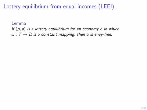
Lottery equilibrium from equal incomes (LEEI)

LemmaIf (p, a) is a lottery equilibrium for an economy e in whichω : T → Ω is a constant mapping, then a is envy-free.

TheoremIf an economy e satisfies either Condition (A) or Condition (B),then there exists a lottery allocation for e that is both envy-freeand Pareto efficient.

Proof.I Reallocate the artificial currency equally across agentsI Reallocate all other goods to the outside endowmentI Compute a lottery equilibrium

16/22

Lottery equilibrium from equal incomes (LEEI)

LemmaIf (p, a) is a lottery equilibrium for an economy e in whichω : T → Ω is a constant mapping, then a is envy-free.

TheoremIf an economy e satisfies either Condition (A) or Condition (B),then there exists a lottery allocation for e that is both envy-freeand Pareto efficient.

Proof.I Reallocate the artificial currency equally across agentsI Reallocate all other goods to the outside endowmentI Compute a lottery equilibrium

17/22

Combinatorial allocationA-LEEI

Setting: a set of goods (e.g. courses) to allocate among a set ofagents (e.g. students) who demand bundles (e.g. schedules)

A-LEEI mechanism:

1. Ask agents to report their utility functions2. Consider a continuum replication of the setting3. Compute a lottery equilibrium from equal incomes, which

determines a lottery for each original agent4. Resolve lotteries and assign agents their bundles

I “Approximate” because there will be some market clearingerror conjectured convergence rates

17/22

Combinatorial allocationA-LEEI

Setting: a set of goods (e.g. courses) to allocate among a set ofagents (e.g. students) who demand bundles (e.g. schedules)

A-LEEI mechanism:

1. Ask agents to report their utility functions2. Consider a continuum replication of the setting3. Compute a lottery equilibrium from equal incomes, which

determines a lottery for each original agent4. Resolve lotteries and assign agents their bundles

I “Approximate” because there will be some market clearingerror conjectured convergence rates

18/22

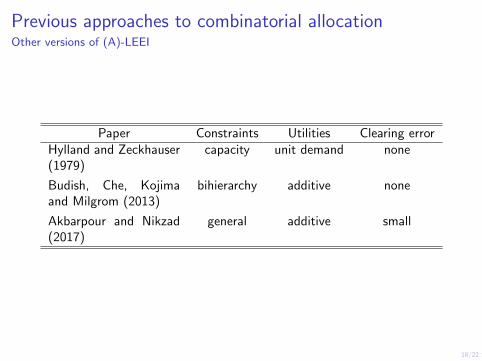
Previous approaches to combinatorial allocationOther versions of (A)-LEEI

Paper Constraints Utilities Clearing errorHylland and Zeckhauser(1979)

capacity unit demand none

Budish, Che, Kojimaand Milgrom (2013)

bihierarchy additive none

Akbarpour and Nikzad(2017)

general additive small

19/22

Previous approaches to combinatorial allocationA-CEEI

I A-CEEI: approximate competitive equilibrium from equalincomes

I Budish (2011)I Budish and Kessler (2016); Budish, Cachon, Kessler and

Othman (2017)

I “Approximate” becauseI there will be some market clearing errorI incomes cannot be perfectly equal

20/22

Social lotteries

I In economies with non-convexities, lotteries concavify indirectutility functions

I efficiency gains (Friedman and Savage, 1948)I strengthens the benefits of social insurance

I Suggests that governments should offer menus of actuariallyfair “social lotteries”

I binary lotteries would sufficeI certain safeguards might be appropriate

21/22

Summary

I With indivisibilities and/or non-convex preferences, it can becostly to prohibit trades of probability shares of bundles

I existenceI first welfare theoremI second welfare theorem

22/22

Next steps

Investigate properties of A-LEEI:

I Bound the rate at which clearing error diminishes in finiteeconomies as the market grows

I Empirical comparison to A-CEEI (Budish and Kessler, 2016)

Explore other applications:

I Dynamic allocation

I Two-sided matching

23/22

Back-Up Slides

24/22

Convergence rates conjecturesback

I Apply the A-LEEI mechanism to the K -fold replication of afixed finite economy

I Clearing error (as a fraction of the total supply) should be

I O(

1√K

)for each good, except with probability that is O(e−K )

I O(

1√K

)for all goods uniformly, except with probability that

is O(e−K

m+n )

25/22

References I

Akbarpour, Mohammad and Afshin Nikzad, “Approximate RandomAllocation Mechanisms,” 2017. https://ssrn.com/abstract=2422777.

Budish, Eric, “The Combinatorial Assignment Problem: ApproximateCompetitive Equilibrium from Equal Incomes,” Journal of Political Economy,2011, 119 (6), 1061–1103.

and Judd Kessler, “Bringing Real Market Participants’ Real Preferencesinto the Lab: An Ex-periment that Changed the Course Allocation Mechanism at Wharton,” 2016.http://faculty.chicagobooth.edu/eric.budish/research/BudishKessler July2016.pdf.

, Gerard Cachon, Judd Kessler, and Abe Othman, “Course Match: ALarge-Scale Implementation of Approximate Competitive Equilibrium fromEqual Incomes for Combinatorial Allocation,” Operations Research, 2017, 65(2), 314–336.

, Yeon-Koo Che, Fuhito Kojima, and Paul Milgrom, “Designing RandomAllocation Mechanisms: Theory and Applications,” The American EconomicReview, 2013, 103 (2), 585–623.

Friedman, Milton and L. J. Savage, “The Utility Analysis of ChoicesInvolving Risk,” Journal of Political Economy, 1948, 56 (4), 279–304.

26/22

References II

Hylland, Aanund and Richard Zeckhauser, “The Efficient Allocation ofIndividuals to Positions,” The Journal of Political Economy, 1979, 87 (2),293–314.

Mas-Colell, Andreu, “Indivisible Commodities and General EquilibriumTheory,” Journal of Economic Theory, 1977, 16 (2), 443–456.

Rogerson, Richard, “Indivisible Labor, Lotteries and Equilibrium,” Journal ofMonetary Economics, 1988, 21 (1), 3–16.

Varian, Hal R, “Equity, Envy and Efficiency,” Journal of Economic Theory,1974, 9 (1), 63–91.