Using Spectral Graph Theory to MapQubits ontoConnectivity-Limited Devices

JOSEPH X. LIN, ERIC R. ANSCHUETZ, and ARAMW. HARROW,Massachusetts Institute of

Technology

We propose an efficient heuristic for mapping the logical qubits of quantum algorithms to the physical qubits

of connectivity-limited devices, adding a minimal number of connectivity-compliant SWAP gates. In particular,

given a quantum circuit, we construct an undirected graph with edge weights a function of the two-qubit

gates of the quantum circuit. Taking inspiration from spectral graph drawing, we use an eigenvector of the

graph Laplacian to place logical qubits at coordinate locations. These placements are then mapped to physical

qubits for a given connectivity. We primarily focus on one-dimensional connectivities, and sketch how the

general principles of our heuristic can be extended for use in more general connectivities.

CCS Concepts: • Hardware→ Quantum computation.

Additional Key Words and Phrases: compilation, spectral graph theory

1 INTRODUCTIONThe field of quantum computation has shown immense promise for solving certain problems more

efficiently than classical computers including prime factorization [21], unstructured search [7],

optimization [5], and chemical simulation [16]. However, while advantageous quantum algorithms

have been thoroughly developed in theory, the technological implementations of quantum devices

is still very much in its infancy. The challenges and resource constraints of current and near-term

devices present roadblocks for the feasibility of practial quantum information processing.

Because quantum entangling operations are crucial to setting quantum computing apart from

classical computing, it is important in many practical algorithms for operations to be applied

between multiple qubits. However, on many present day quantum architectures, the application of

multiqubit gates is not always possible among every subset of qubits. This particular challenge

has to do with the connectivity limitation of physical devices, which constrains the set of allowable

operations. Therefore, there is a compilation step needed to convert a theoretical quantum algorithm,

which often assumes full connectivity between qubits, to an equivalent connectivity compliantcircuit that can be run on a physical device. In this work, we focus on this challenge and develop a

novel approach using spectral graph theory.

In Sec. 2, we provide the background and motivation for our problem. This includes formally

describing the problem of converting quantum circuits to be compliant with the connectivity

constraints of a device, surveying prior solutions to the problem, and reviewing relevant results

from spectral graph theory. Next, we explain our algorithm in Sec. 3, discussing design principles

that motivate our decisions, specific details for practical implementation, and overall runtime. In

Sec. 4 we discuss the use of known benchmarks and a comparable open source algorithm to evaluate

our own algorithm, and show the results in Sec. 5. Finally, we conclude in Sec. 6 and provide future

directions for improvement.

2 BACKGROUNDIn this section, we provide the necessary background for our algorithm. We first formalize the

problem of making a quantum circuit connectivity-compliant for a given device. Then, we survey

Authors’ address: Joseph X. Lin, joelin@mit.edu; Eric R. Anschuetz, eans@mit.edu; Aram W. Harrow, aram@mit.edu,

Massachusetts Institute of Technology, 77 Massachusetts Avenue, Cambridge, Massachusetts, 02139.

arX

iv:1

910.

1148

9v1

[qu

ant-

ph]

25

Oct

201

9

2 Lin, Anschuetz, and Harrow

related work on the problem, and close with a description of spectral graph theory and token

swapping, two key components to our algorithm.

2.1 Problem DescriptionAs mentioned in Sec. 1, our objective is to start with a circuit containing only single qubit and

CNOT gates, with no connectivity constraints, and transform the circuit into one adhering to the

connectivity constraints of the device. To differentiate the two domains, we call the untransformed

circuit the logical circuit and the transformed circuit the physical circuit. We say that the logical

circuit operates on logical qubits with logical gates, and similarly for the physical circuit.

For this transformation to be meaningful, the circuits must be equivalent in the sense that their

unitary descriptions are equal. There are certain operations that can be performed that lead to

equivalent circuits in all cases. These include:

(1) the commutation of disjoint gates. When two gates operate on disjoint subsets of qubits, the

order in which they are applied does not matter.

(2) the logical reordering of qubits. Circuits are equivalent under the relabling of qubits.

(3) the physical reordering of qubits. When a SWAP gate is inserted for qubits i and j , and gates

and measurements are changed to take the SWAP into account, the circuit is equivalent.

See [15] for a longer and more thorough list of circuit equivalences. We assume that the first two

operations can be done with no cost, but that the addition of SWAP gates should be minimized to

save resources and to minimize the effects of noise in physical implementations of the circuit.

We are now ready to formalize the connectivity-compliance problem. As previously discussed,

only multi-qubit gates of the circuit are affected by connectivity; therefore, without loss of generality

we consider only the CNOT gates of a circuit. Let Q be the set of logical qubits of the circuit, with

M ≡ |Q |. Similarly, let the set C be the CNOTs of a logical circuit, with N ≡ |C |. We can represent

C as an ordered list of pairs

[ (lc1, l t1

), . . . ,

(lcN , l

tN

) ], where lci ∈ Q and l ti ∈ Q are the logical control

and target qubits, respectively, of the i-th CNOT.

Next, we represent the connectivity characteristics of an architecture by a graph G = (V ,E),where the vertices are the physical qubits and the edges represent pairs of qubits which support

two qubit operations. We assume |V | = M . We also assume that the graph is unweighted and

undirected, meaning each edge can support a CNOT in either direction and can do so with equal

“ability” (e.g. fidelity, time, etc.) as any other edge.

Now, let C ′be the ordered list of two-qubit gates of another circuit, where N ′ = |C ′ |. It also

can be represented as an ordered list of tuples

[ (p11,p2

1, type

1

), . . . ,

(p1N ′,p2N ′, typeN ′

) ], where typei

represents the type of gate that gate i is (i.e. either CNOT or SWAP), and p1i ,p2

i ∈ V represent the

two physical qubits on which the gate is applied.

If we can transform circuit C to C ′using the three equivalency rules established above, then the

circuits are equivalent. Furthermore, if the physical qubits on each gate of C ′are connected, i.e.(

p1i ,p2

i)∈ E for all i , then the transformed circuit is connectivity compliant according toG . We will

deem a transformation valid if an only if both criteria are satisfied: the transformed circuit must be

both equivalent to the original circuit and also compliant to the connectivity rules.

Finally, our objective is to find a valid C ′that minimizes N ′

; as C and C ′must have the same

number of CNOTs assuming C ′was constructed using the aforementioned circuit transformation

rules then, by construction, this optimization minimizes the total number of added SWAP gates.

A couple notes should be made about theC ′we consider. First, no transformed circuit should have

a SWAP gate that can be commuted to the front of the circuit. This is because another equivalent

and still valid circuit can be made by replacing that SWAP with a logical relabeling (that is, using

transformation rule 2 instead of 3). Similarly, no SWAP gates should be able to be commuted to the

Using Spectral Graph Theory to MapQubits onto Connectivity-Limited Devices 3

end of the circuit. This is because these SWAP gates can be removed and any single qubit gate or

measurements happening at the end of the circuit can be logically reassigned.

To finish our problem description, we discuss two different ways to view the transformation

problem. The first is SWAP based, and is essentially how we described this problem: add SWAP

gates toC (and adjust any affected gates that follow) until the resultingC ′is connectivity-compliant.

Implicit in this was also deciding on an initial one-to-one logical relabeling π0 : Q → V , which is

the mapping at the beginning of C ′.

The second interpretation is layer and permutation based. Note thatC ′can be viewed as layers of

CNOT gates which can be applied using variousQ → V permutations, with the intermediate SWAP

gates acting as a bridge between permutation. This can be seen as follows. Suppose we tookC ′, and

commuted the gates so that as many CNOTs were at the front as possible before a SWAP gate must

be applied. Then, those CNOTs are the CNOTs from C ′that can be made connectivity compliant

through the initial mapping π0. Then, suppose that we remove those CNOTs from the circuit (as

they have been now applied already), and perform a similar commutation to bring as many SWAPs

to the front as possible. These SWAPs form a physical permutation σ1 : V → V . If we then remove

the SWAPs and again bring as many CNOTs to the front as we can, we have another layer of CNOTs

that can be applied from the logical circuit, under the permutation π1 = σ1π0 : Q → V . This can be

continued until all gates of C ′are exhausted.

Using this second interpretation, we can describe an equivalent way of transforming C into a

valid C ′:

(1) Beginning with C , allow commutation of CNOTs that are nonoverlapping.

(2) Partition the CNOTs into layers such that the CNOTs of each layer can be made compliant

using some mapping πi : Q → V .

(3) Using only compliant SWAP gates, create a physical permutation σi+1V → V that transfers

one logical permutation to the next one, via πi+1 = σi+1πi .

The optimization problem is still the same, find the C ′with the fewest number of added SWAPs,

but the optimizaiton is now over layers and permutations, rather than individual SWAPs. As we

will see, this interpretation can allow for the overall optimization problem to be subdivided into

smaller problems with well-known solvers.

2.2 Prior WorkIn the literature, results and algorithms related to this issue of connectivity-compliance have gone

by many names, including circuit layout, circuit transformation, qubit allocation, qubit mapping,

and qubit routing [1, 3, 6, 11, 14, 18, 20, 22, 24, 25]. We provide a survey of these results, and go

more in-depth with a few of particular interest.

First, we establish the various choices that each algorithm designer has had to make:

(1) Metric to optimize. Examples include circuit size (i.e. number of gates in the final circuit;

often equivalent to number of added SWAP gates); circuit depth (number of layers in the

circuit, where each qubit is acted on by only one gate per layer); and error rate.(2) Exact vs. Approximate. Designers must make the choice between a brute force approach

versus using a heuristic or relaxation.(3) Connectivity Constraint. Examples include LNN, 2D grid nearest neighbor, connectivities of

actual NISQ devices; ring; and arbitrary connectivity

(4) Problem Interpretation. As described above, two common interpretations are SWAP-basedand layer- and permutation-based.

4 Lin, Anschuetz, and Harrow

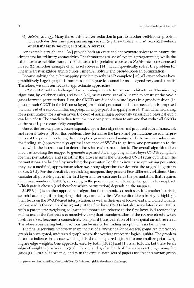
(5) Solving strategy. Many times, this involves reduction in part to another well-known problem.

This includes dynamic programming; search (e.g. breadth-first and A* search); Booleanor satisfiability solvers; andMinLA solvers.

For example, Siraichi et al. [22] provide both an exact and approximate solver to minimize the

circuit size for arbitrary connectivity. The former makes use of dynamic programming, while the

latter uses a search-like procedure. Both use an interpretation close to the SWAP-based one discussed

in Sec. 2.1. Another example of an exact solver is [24], which specifically solves the problem for

linear nearest-neighbor architectures using SAT solvers and pseudo-Boolean optimization.

Because solving the qubit mapping problem exactly is NP-complete [12], all exact solvers have

prohibitively large asymptotic runtimes, and in practice cannot be used beyond very small circuits.

Therefore, we shift our focus to approximate approaches.

In 2018, IBM held a challenge1for compiling circuits to various architectures. The winning

algorithm, by Zulehner, Paler, and Wille [25], makes novel use of A* search to construct the SWAP

gates between permutations. First, the CNOTs are divided up into layers in a greedy fashion (i.e.

putting each CNOT in the left-most layer). An initial permutation is then needed; it is proposed

that, instead of a random initial mapping, an empty partial mapping is used. Then when searching

for a permutation for a given layer, the cost of assigning a previously unassigned physical qubit

can be made 0. The search is then from the previous permutation to any one that makes all CNOTs

of the next layer connectivity compliant.

One of the second place winners expanded upon their algorithm, and proposed both a framework

and several solvers [3] for this problem. They formalize the layer- and permutation-based interpre-

tation of the problem, defining the concepts of permuters and mappers. The former is a subroutine

for finding an (approximately) optimal sequence of SWAPs to go from one permutation to the

next, while the latter is used to determine what each permutation is. The overall algorithm then

involves invoking the mapper to generate a permutation, applying all first-layer CNOTs compliant

for that permutation, and repeating the process until the unapplied CNOTs run out. Then, the

permutations are bridged by invoking the permuter. For their circuit size optimizing permuter,

they use a modified, approximate token swapping algorithm (we describe the original algorithm

in Sec. 2.3.2). For the circuit size optimizing mappers, they present four different variations. Most

consider all possible gates in the first layer and for each one finds the permutation that requires

the fewest number of SWAPs, according to the permuter, while allowing that gate to be compliant.

Which gate is chosen (and therefore which permutation) depends on the mapper.

SABRE [11] is another approximate algorithm that minimizes circuit size. It is another heuristic,

search-based algorithm targeting arbitrary connectivities. We mention them briefly to highlight

their focus on the SWAP-based interpretation, as well as their use of look-ahead and bidirectionality.

Look-ahead is the notion of using not just the first layer CNOTs but also some later layer CNOTs,

with a parametric weighting to lower its importance relative to the first layer. Bidirectionality

makes use of the fact that a connectivity compliant transformation of the reverse circuit, when

itself reversed, becomes a connectivity compliant transformation of the original circuit reversed.

Therefore, considering both directions can be useful for finding an optimal transformation.

The final algorithms we review share the use of a interaction (or adjacency) graph. An interaction

graph is a weighted, undirected graph where the vertices represent logical qubits. The graph is

meant to indicate, in a sense, which qubits should be placed adjacent to one another, prioritizing

higher edge weights. One approach, used by both [18, 20] and [1], is as follows. Let there be an

edge of weightwi j between logical qubits qi and qj if and only if there are exactlywi j two-qubit

gates (i.e. CNOTs) between qi and qj in the circuit. Both sets of papers use this interaction graph

1https://www.ibm.com/blogs/research/2018/08/winners-qiskit-developer-challenge/

Using Spectral Graph Theory to MapQubits onto Connectivity-Limited Devices 5

to map the logical qubits onto an LNN architecture. While the former set of two papers use the

interaction graph and solves a Minimum Linear Arrangement (MinLA) problem, the latter paper

performs a graph partitioning algorithm on the interaction graph.

In future Sections, we will refer back to this survey to compare and contrast the design, imple-

mentation, and performance of our own algorithm.

2.3 Theory BackgroundTo close this Section, we will describe the necessary theoretical background on which we will

base our own algorithm. We describe the use of spectral graph theory for assigning points of a

graph to coordinate locations, as well as the token swapping problem for transitioning between

permutations via swapping. These have the significance of providing ways to generate the logical

permutations πi : Q → V and physical permutations σi : V → V , respectively, that were described

in Sec. 2.1.

2.3.1 Spectral Graph Theory and Drawing. Here, we discuss a method for mapping the vertices of

a weighted graph to Cartesian coordinate locations, given that the edge weights are some sort of

priority for how close the vertices should be. We develop this method and make the description

more precise below.

Let G =(V , E

)be a weighted, undirected graph with vertices vi for i = 1, . . . ,n. Next, suppose

that a nonnegative weightwi j = w ji is associated between each pair of vertices vi and vj , where

i , j. If(vi , vj

)∈ E is an edge, then wi j > 0; otherwise, wi j = 0. The Laplacian of G can then be

defined as follows:

Definition 2.1. (GraphLaplacian) The Laplacian of a graph G =(V , E

)is defined by a symmetric,

n × n matrix L such that:

Li j =

∑k,i

wik , if i = j

−wi j , if i , j(1)

Note that L can also be written as D −A, where D and A are the degree and adjacency matrices,

respectively, of G.Citing [10], there are several properties of the Laplacian that make it appealing for our purposes.

In particular, its eigenvectors help provide a drawing for the graph that places the vertices at spatial

locations while optimizing over a quantity related to the edge weights. First, consider the following

result:

Lemma 2.2. Let x ∈ Rn . Then

xTLx =∑i<j

wi j(xi − x j

)2

. (2)

Since this is a standard fact, we postpone the proof to Appendix A.

Next, it can be directly observed that L is a real, symmetric matrix. It can further be easily shown

that L is positive semidefinite. This allows us to conclude that L has nonnegative, real eigenvalues

and real, orthogonal eigenvectors. The lowest eigenvalue is always 0, regardless of the graph.

Lemma 2.3. Let 1n = (1, . . . , 1)T ∈ Rn be the all ones vector. Then:

L1n = 0, (3)

i.e. 1n is an eigenvector with eigenvalue 0.

6 Lin, Anschuetz, and Harrow

Again the proof of this well-known property is in Appendix A.

Finally, we are ready to motivate an optimization problem relating L to drawing a graph. Suppose

the edge weight wi j is a measure of “how important” it is for vertices vi and vj to be near one

another, with a larger weight correlating with greater importance. Next, suppose we seek to layout

the vertices in 1D according to a vector x ∈ Rn , with vi at location xi . A reasonable minimization

problem would then be:

min

x

∑i<j

wi j (xi − x j )2 (4)

s.t. Var(x) =1

n. (5)

Note that the constraint is simply chosen to normalize the scale of the drawing; the choice of 1/n is

completely arbitrary but helps simplify the calculations in the following steps. Next, notice that we

can use Lemma 2.2 to rewrite the problem as:

min

xxTLx (6)

s.t. Var(x) = 1/n. (7)

We then invoke Lemma 2.3 to note that both the objective and variance do not change under a

translational shift; that is, both x and x + α1n for any α have the same variance and same objective

value. Therefore, without loss of generality we choose for x t 1n = 0, i.e. that the average position is

0. This is, again, an arbitrary choice made out of convenience, as it allows us to write:

Var(x) = xTx/n. (8)

Combining all of these results, we can write our desired optimization problem as:

min

xxTLx (9)

s.t. xTx = 1 (10)

xT 1n = 0. (11)

Define the eigenvalues of L to be 0 = λ1 ≤ λ2 ≤ · · · ≤ λn with corresponding normalized

eigenvectors 1n/√n = y(1),y(2), . . . ,y(n). As our optimization problem is to minimize the Rayleigh

quotient R (L,x) = xTLx , subject to x being normalized and over the subspace orthogonal to the

eigenvector y(1), we can invoke the Courant–Fischer principle and immediately write down that

y(2) is an optimal solution with optimal objective value λ2. This special vector is known as the

Fiedler vector of G.To conclude this section, we note a couple extensions of this result. First, suppose we only

allowed for the vertices to be placed at discrete locations, e.g. integer locations. Formally, suppose

we required a one-to-one mapping π : V → {1, 2, . . . ,n}. A natural way to get an approximate

solution is to take the components of y(2) and use the order they impose:

π (vi ) > π(vj)only if y(2)i ≥ y(2)j .

We cite [8, 9, 19] for this result, which show that this mappings gives a good approximation to

the related Minimum Linear Arrangement (MinLA) problem. Note that in the MinLA problem, the(xi − x j

)2

terms are replaced by

��φ (vi ) − φ(vj) ��terms. We cite this result, not because we wish to

solve the MinLA problem, but because, as we previously mentioned, MinLA solvers have been used

in part for approximate solvers. Therefore, we are motivated to use a solver as an alternative but

related heuristic.

Using Spectral Graph Theory to MapQubits onto Connectivity-Limited Devices 7

Finally, although we will mostly focus on using the 1D result, we note that this spectral drawing

method can be expanded to two (or even more) dimensions. To do this, we again cite [10], which

motivates the use of y(3) for the second dimension. This vector solves the same optimization

problem, but with the added constraint that x is orthogonal to y(2) as well. This provides a drawingin which the two dimensions are uncorrelated, which allows for the added dimension to provide

as much new information as possible. While this is useful for drawing purposes, the use of this

method to map to discrete grid locations in two dimensions is less trivial than the one-dimensional

case.

2.3.2 Token Swapping. We now discuss the subroutine that will be used to transfer logical qubits

from one permutation to another using only connectivity compliant SWAP gates. Our problem is

exactly equivalent to the Token Swapping Problem, which can be described as follows.

Suppose we have a graphG = (V ,E) of n vertices. Further suppose that we have tokens t1, . . . , tnthat are to be placed on the vertices so that each vertex has exactly one token. Given an initial and

desired final mapping of tokens to graph vertices, the problem is then to transform the former to

the latter only by swapping the tokens on a pair of vertices connected by an edge.

This is exactly analogous to the connectivity compliance problem for quantum circuits: the

verticesV represent physical qubits, the edges E are between physical qubits which allow two-qubit

operations, and the tokens are the logical qubits to be mapped on the physical devices. Swapping

adjacent tokens then amounts to applying SWAP gates between adjacent qubits.

This problem is NP-hard, and the best known exact algorithm requires an exponential runtime.

Therefore, we use an approximate algorithm described in [13] that gets a sequence of swaps of

length within 4 times the optimal length for general graphs, and within 2 times the optimal length

for trees. For completeness, we review the algorithm in Appendix B.

3 THE SPECTRAL MAPPING ALGORITHM3.1 Design Principles and MotivationsThe related work and subroutines outlined in Sec. 2 motivate the design our algorithm. We start by

specifying the five general categories we previously listed as choices for algorithm designers.

First, we will be focusing on an approximate solution. As previously discussed, an exact solution

takes exponentially long to solve for (and often requires exponential space as well); this is not

feasible for circuits consisting of more than just a few qubits and CNOTs. Next, we adhere to the

permutation-based interpretation of the problem, specifically the mapper-permuter model from [3].

This provides the problem with added structure and modularity, which in turn allows us to design

and evaluate smaller subproblems independently. Like [3], we will use the approximate token

swapping algorithm as our permuter, which we described in Sec. 2.3.2.

Next, we consider the choice of mapper. Note that here we only describe the high-level design,

omitting details that will be presented in later sections. We are motivated by [1, 18, 20] in the

creation of a weighted interaction graph. However, where previous uses of interaction graphs

do not account for how “far” in the future a CNOT occurrence happens, we incorporate a time

component in our interaction graph construction. For example, a CNOT within the earliest layer of

the circuit that acts on the same qubit(s) as many later CNOTs (i.e. a CNOT that is “blocking” many

other gates and acting as a bottleneck) should be given higher priority in qubit placement than a

CNOT near the end of the circuit. In fact, CNOTs many layers back should not be considered at all,

as they are “shielded” from affecting the current permutation we wish to generate by earlier CNOTs.

Therefore, while we do look-ahead past the first layer, we limit how far we look and down-weight

less important CNOTs. We mention at this point that limiting the look-ahead also has the added

benefit of improving runtime; we further discuss this in Sec. 3.5. Finally, we must also consider

8 Lin, Anschuetz, and Harrow

the previous permutation we chose. Therefore, adjacency of the previously chosen permutation is

incorporated into the interaction graph as well.

After the creation of the interaction graph, we make use of spectral graph theory, as described in

Sec. 2.3.1. Note that this gives a mapping of each logical qubit onto a coordinate location according

to the graph Laplacian eigenvectors, which can then in turn be used to place the qubits at discrete

integer locations. As we have already seen other algorithms make use of the MinLA problem [18, 20]

and graph partitioning [1], we believe the related spectral graph drawing method provides another

good solving strategy to the qubit mapping problem.

Like with the other algorithms that have used an interaction graph, our use of spectral graph

theory leads us to focus on the linear nearest neighbor architecture. We do not see this as a

prohibitive restriction on the problem; as described in Sec. 1, many experimental devices do in fact

adhere to LNN connectivity. Furthermore, because LNN connectivity is among themost restrictive of

architectures, finding an efficient translation to an LNN compliant circuit implies the original circuit

can be run efficiently on many other practical, and often less restrictive, architectures [2]. Lastly,

since many analyses have been done on LNN architectures and most qubit mapping algorithms

can run with LNN connectivity constraints, comparison of our results to others can be used to

specifically evaluate our solving strategy choices (i.e. using a weighted interaction graph and

a spectral graph drawing mapper). These reasons all justify and motivate our focus on LNN

architectures.

3.2 Spectral MapperIn this section, we formally detail our spectral mapper.

3.2.1 CNOT Dependency and Layering. Let C be the CNOTs of a logical circuit. The CNOTs of Chave a dependency in that, for i < j , CNOT j must be applied strictly later than CNOT i if there is aqubit both CNOTs act on. In other words, CNOT j cannot be commutated ahead of CNOT i . We say

that CNOT i is a direct blocker of CNOT j if:

(1) i < j,(2) they both act on qubit qk , and(3) no CNOT between i and j acts on qk .

Let b (j) be the set of direct blockers of CNOT j. In general, b (j) can have 0, 1 or 2 elements.

Next, we define tfj , the forward layer of CNOT j. It is a quantity that represents the minimum

number of CNOT layers that must be applied before CNOT j is eligible to be applied. It acts as aproxy for how “soon” the CNOT can be applied. Formally, we have:

tfj =

0, if |b (j)| = 0

1 + max

i ∈b(j)tfi , otherwise

. (12)

If we think about assigning each CNOT a layer, where each layer contains CNOTs that can be

simultaneously applied, tfj represents the layer of CNOT j in a greedy layering that tries to place

each CNOT as early as possible. If we consider all the CNOTs j for which tfj = 0, one of them will

be the next CNOT to be applied. We will call this set of CNOTs the front layer.Consider now the reverse list of C , given by

[ (lcN , l

tN

), . . . ,

(lc1, l t1

) ]. We similarly define trj , the

reverse layer of CNOT j, as the forward layer of CNOT j in this reversed list. Let T = maxi tfi be

the maximum forward layer. Then, the quantity T − t tj represents the layer of CNOT j in a lazy

layering of C that tries to place each CNOT as late as possible.

Using Spectral Graph Theory to MapQubits onto Connectivity-Limited Devices 9

We interpret these results as follows. A small forward layer means the CNOT is soon to be eligible

for application, and has the potential to be related to the next mapping of logical to physical qubits.

A simultaneously small reverse layer, however, means that the CNOT could in fact be applied much

later, and have little to do with the next mapping. These concepts are used when calculating our

weighted interaction graph.

3.2.2 Weighted Interaction Graph. A weighted interaction graph is some weighted, undirected

graph G =(Q, E

)whose vertices are logical qubits, and whose edge weights wi j represent the

priority of placing those qubits close to one another. There are two categories of contributions

to edge weights: the previous logical to physical mapping, and the CNOTs yet to be applied. We

consider each one.

First, suppose the previous permutation is given by π : Q → V . For simplicity, we will let

V = {1, 2, . . . ,M}, and order the vertices so that the LNN connectivity constraint places consecutive

numbers adjacent to each other. That is, for i, j ∈ V ,

(i, j) ∈ E if and only if |i − j | = 1. (13)

Then, for every qi ,qj ∈ Q for which

(π (qi ) ,π

(qj) )

∈ E, i.e. for each pair of logical qubits that

were previously adjacent, we incrementwi j by the prior mapping weight β ∈ [0, 1]. The motivation

is that, to minimize the number of SWAPs, the next permutation we generate should be as close to

the previous as possible. The parameter then acts as a sort of memory for the algorithm. It adds a

β-weighted component of the previous logical adjacency to G.Next, we consider the unapplied CNOTs, which we will represent as C . Each CNOT can only be

applied if the qubits they act on are adjacent. Furthermore, at least one CNOT should be applied in

the next generated permutation, and at least one must come from the front layer. As reasoned in

Secs. 3.1 and 3.2.1, we can consider CNOTs with a small forward layer to potentially be applied in

the next mapping, while discounting those same CNOTs with large backward layers due to the

flexibility in their layer choice. We define an integer τ ∈ [0,T ] to be the cutoff layer and real number

α ∈ [0, 1] to be the layering discount. Then, if CNOT i acts on qubits qj and qk and has forward

layer tfi ≤ τ , we incrementw jk by αT−t

ri .

In closed form, we define the edge weight between qj and qk as:

w jk =∑

i :{lci ,l ti }={qj ,qk }t fi ≤τ

αT−tri +

{β if

(π(qj),π (qk )

)∈ E

0 otherwise

. (14)

We intend to use this interaction graph G as an input to the spectral drawing method outlined in

Section 2.3.1. A mapping π : Q → V is generated, placing the logical qubits at physical locations.

While we have chosen the edge weights of G to try to place the qubit pairs in front layer CNOTs

close together, there is actually no guarantee that any front layer CNOTs are actually compliant on

the generated mapping. This leads to a breakdown that needs to be resolved via some fallback. A

naive fallback would be to arbitrarily pick a front layer CNOT and SWAP the two qubits together,

or to apply another established algorithms. In the following section, we propose a third strategy,

which we ultimately use.

3.2.3 Forced Coupling. For our fallback strategy, we would like to make use of our weighted

interaction graph and spectral drawing framework. However, we wish to guarantee that the

generated permutation allows for at least one front layer CNOT to be compliant. To this end, we

propose a forced coupling step. First, we consider the front layer CNOTs with the largest reverse

10 Lin, Anschuetz, and Harrow

layers, signifying the highest priority of application within our previous description. We use this

limited subset of the front layer, rather than the whole front layer, to minimize the impact of the

fallback and only apply this forceful coupling to priority pairs of qubits.

More specifically, we are seeking every CNOT i for which tri = T . Then, if that CNOT i is

applied on qubits qj and qk , we combine the corresponding vertices in G together. This combination

involves:

(1) replacing qj and qk with a single node fused node f representing the two qubits, and

(2) for every third node p (which may be a single qubit or a newly created fused node), drawing

an edge between f and p with edge weight equal to the sum of the previous edge weights

between qj and p, and between qk and p.

After this process is performed for every CNOT i with tri = T , we are left with a new interaction

graph Gf orced =(Q f orced , Ef orced

).

Note that because no front layer CNOTs act on the same qubit, each new vertex in Q f orced

represents either one or two of the original qubits from Q . We then again use the spectral drawing

method, but with Gf orcedas the input.

This method will first provide us with a real number coordinate position for each vertex in

Q f orced. For each coordinate, we first add a small perturbation, randomly generated for each vertex,

so as to break ties; we do this to guarantee the forced pairs will be adjacent to each other. Then, we

assign each of the original qubits from Q to the coordinate of their corresponding forced vertex in

Q f orced; note that forced pairs are thus given the same location. Finally, if yi is the coordinate for

qi , we generate the permutation π : Q → V adhering to

π(qj)> π (qk ) =⇒ yj ≥ yk . (15)

Note that the ties between the forced pairs is broken at random, as any such ordering of the pairs

will satisfy Eq. 15.

By virtue of the forced pairs selection, at least one of the front layer CNOTs is connectivity

compliant on π , and therefore the overall algorithm can progress.

One interesting consideration is whether this forced pairing algorithm can be used independently,

as a standalone mapper, rather than as a fallback. This is an option we consider and allow for our

overall algorithm.

3.2.4 Applying the Spectral Drawing Algorithm. We conclude our description of our spectral mapper

by discussing some details regarding the use of the spectral drawing method from Sec. 2.3.1. As

mentioned, the coordinates generated may sometimes lead to vertices assigned to the same location.

In that case, ties are typically broken at random, either implicitly when moving the vertices to

discrete integer locations, or explicitly through the addition of small, random perturbations to each

coordinate.

Another consideration we make is in regards to the symmetries of our architecture. In particular,

a given mapping to an LNN architecture affords the same connectivity constraints when rotated

180◦(or reflected about its center). As a result, we must consider both possibilities; this is equivalent

to considering the mapping induced by both the Fiedler vector y(2) calculated by the eigensolver,

and its negative −y(2). The mapping we ultimately choose is the one which requires the fewest

SWAPs to get from the previous permutation; as a proxy, we use as a metric the sum of the distances

each logical qubit must travel from previous to potential mapping, and pick the potential mapping

with the smaller sum as the generated mapping.

Using Spectral Graph Theory to MapQubits onto Connectivity-Limited Devices 11

3.3 BidirectionalityMany of the algorithms we have considered start from the beginning of the circuit, as it is provided,

and then sequentially work to the end in the forward direction. When considering the connectivity

compliance problem on a circuit of CNOTs, however, the same problem can be solved on the reversed

circuit to provide a valid transformation. Indeed, there is no inherent preference between the two

directions. Thus, we explore the option of a bidirectional mapper. At each iteration, the mapping

strategy is applied as described in Sec. 3.2 to generate a mapping π that allows for some front layer

CNOTs to be applied. Our bidirectional proposal adds for the same iteration the generation of a

mapping on the reversed circuit as well, so that some front layer CNOTs on the reversed circuit

can be applied. In terms of the notation for generating the weighted dependency graph, the reverse

mapper simply interchanges tfi and tri . The mappings are then generated for each end of the circuit

every iteration, working towards the middle of the circuit.

3.4 Overall Connectivity-Compliance Transformation AlgorithmIn this section, we summarize the full algorithm for transforming a logical circuit into one that is

LNN compliant. First, we list the configuration options we have available for our algorithm. These

include whether to use the forced-coupling mapper as a standalone or fallback strategy; whether to

include bidirectionality; and what choices of α , β , and τ to choose. A summary of the options is

given in Table 1.

Parameter Description Values

Forced-coupling Whether the mappings are exclusively based on

the forced-coupling weighted interaction graph,

or if the forced-coupling case is only used as a fall-

back for the regular weighted interaction graph.

{Standalone, Fallback}

Direction Which direction(s) the iterations traverse through

the circuit.

{Forward, Bidirec-

tional}

α The layering discount factor used in calculating

the weighted interaction graph. It is meant to di-

minish the impact of CNOTs that can be pushed

back to much later layers.

Any real in [0, 1]

β The prior mapping weight used in calculating the

weighted interaction graph. It is meant to weight

the relative importance of remaining close to the

previous mapping.

Any real in [0, 1]

τ The cutoff layer used in calculating the weighted

interaction graph. It is meant to limit the layers of

look-ahead.

Any positive integer

Table 1. A summary of all possible configuration options for our overall circuit transformation algorithm.

We begin with a logical circuit C , consisting of N CNOT gates andM qubits. Until we run out

of unapplied CNOTs, we perform the following iteration. First, we run our spectral mapper, as

described in Sec. 3.2, using our specified configurations. This involves the creation of a weighted

interaction graph, the use of spectral graph theory to label each logical qubit to a coordinate, and

the ordering of logical qubits into discrete locations on an LNN architecture. Note that for the

first iteration, no previous mapping is used for the interaction graph. By design, some front layer

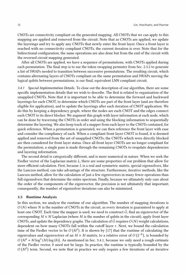
12 Lin, Anschuetz, and Harrow

CNOTs are connectivity compliant on the generated mapping. All CNOTs that we can apply to this

mapping are applied and removed from the circuit. Note that as CNOTs are applied, we update

the layerings and try to apply any CNOTs that newly enter the front layer. Once a front layer is

reached with no connectivity compliant CNOTs, the current iteration is over. Note that for the

bidirectional configuration, the same operations are also done but from the end of the circuit with

the reversed circuit mapping generated.

After all CNOTs are applied, we have a sequence of permutations, with CNOTs applied during

each permutation. The final step is to use the token swapping permuter from Sec. 2.3.2 to generate

a list of SWAPs needed to transition between successive permutations. The resulting circuit, which

contains alternating layers of CNOTs compliant on the same permutation and SWAPs moving the

logical qubits between permutations, is our final, equivalent LNN compliant circuit.

3.4.1 Special Implementation Details. To close out the description of our algorithm, there are some

specific implementation details that we wish to describe. The first is related to organization of the

unapplied CNOTs. Note that it is important to be able to determine the forward and backward

layerings for each CNOT, to determine which CNOTs are part of the front layer (and are therefore

eligible for application), and to update the layerings after each iteration of CNOT application. We

do this by keeping a dependency graph, where the nodes are each CNOT and the edges connect

each CNOT to its direct blocker. We augment this graph with layer information at each node, which

can be done by traversing the CNOTs in order and using the blocking information to sequentially

determine the layering. We also keep track of a mapper from each layer to the CNOTs contained, for

quick reference. When a permutation is generated, we can then reference the front layer with ease

and consider the compliancy of each. When a compliant front layer CNOT is found, it is deemed

applied and removed from the set of unapplied CNOTs; the CNOTs which were directly blocked

are then considered for front layer status. Once all front layer CNOTs are no longer compliant for

the permutation, a single pass is made through the remaining CNOTs to reupdate dependencies

and layering information.

The second detail is categorically different, and is more numerical in nature. When we seek the

Fiedler vector of the Laplacian matrix L, there are some properties of our problem that allow for

more efficient calculation. First, because L is a real and symmetric matrix, special eigensolvers, like

the Lanczos method, can take advantage of the structure. Furthermore, iterative methods, like the

Lanczos method, allow for the calculation of just a few eigenvectors in many fewer operations than

full eigensolvers that determine the entire spectrum. Finally, because we ultimately only care about

the order of the components of the eigenvector, the precision is not ultimately that important;

consequently, the number of eigensolver iterations can also be minimized.

3.5 Runtime AnalysisIn this section, we analyze the runtime of our algorithm. The number of mapping iterations is

O (N ) where N is the number of CNOTs in the circuit, as every iteration is guaranteed to apply at

least one CNOT. Each time the mapper is used, we need to construct G, find an eigenvector of the

correspondingM ×M Laplacian (whereM is the number of qubits in the circuit), apply front layer

CNOTs, and update the dependency graphs. The calculation of G requiresO (N )weight calculations,dependent on how many CNOTs fall within the cutoff layer τ . Next, we bound the calculation

time of the Fiedler vector to be O(M3

). It is shown by [17] that the runtime of calculating the

eigenvalues and eigenvectors of an M × M matrix, to a relative error of O(2−b )

, is bounded by

O(M3 +M log

2 (M) log (b)). As mentioned in Sec. 3.4.1, because we only need a rough estimate

of the Fiedler vector, b need not be large. In practice, the runtime is typically bounded by the

O(M3

)term. Second, we note that in practice we only require a few iterations of an iterative

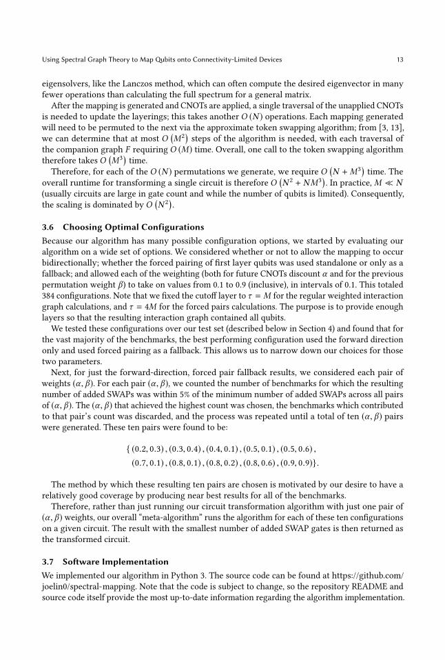
Using Spectral Graph Theory to MapQubits onto Connectivity-Limited Devices 13

eigensolvers, like the Lanczos method, which can often compute the desired eigenvector in many

fewer operations than calculating the full spectrum for a general matrix.

After the mapping is generated and CNOTs are applied, a single traversal of the unapplied CNOTs

is needed to update the layerings; this takes another O (N ) operations. Each mapping generated

will need to be permuted to the next via the approximate token swapping algorithm; from [3, 13],

we can determine that at most O(M2

)steps of the algorithm is needed, with each traversal of

the companion graph F requiring O (M) time. Overall, one call to the token swapping algorithm

therefore takes O(M3

)time.

Therefore, for each of the O (N ) permutations we generate, we require O(N +M3

)time. The

overall runtime for transforming a single circuit is therefore O(N 2 + NM3

). In practice,M ≪ N

(usually circuits are large in gate count and while the number of qubits is limited). Consequently,

the scaling is dominated by O(N 2

).

3.6 Choosing Optimal ConfigurationsBecause our algorithm has many possible configuration options, we started by evaluating our

algorithm on a wide set of options. We considered whether or not to allow the mapping to occur

bidirectionally; whether the forced pairing of first layer qubits was used standalone or only as a

fallback; and allowed each of the weighting (both for future CNOTs discount α and for the previous

permutation weight β) to take on values from 0.1 to 0.9 (inclusive), in intervals of 0.1. This totaled

384 configurations. Note that we fixed the cutoff layer to τ = M for the regular weighted interaction

graph calculations, and τ = 4M for the forced pairs calculations. The purpose is to provide enough

layers so that the resulting interaction graph contained all qubits.

We tested these configurations over our test set (described below in Section 4) and found that for

the vast majority of the benchmarks, the best performing configuration used the forward direction

only and used forced pairing as a fallback. This allows us to narrow down our choices for those

two parameters.

Next, for just the forward-direction, forced pair fallback results, we considered each pair of

weights (α , β). For each pair (α , β), we counted the number of benchmarks for which the resulting

number of added SWAPs was within 5% of the minimum number of added SWAPs across all pairs

of (α , β). The (α , β) that achieved the highest count was chosen, the benchmarks which contributed

to that pair’s count was discarded, and the process was repeated until a total of ten (α , β) pairswere generated. These ten pairs were found to be:

{ (0.2, 0.3) , (0.3, 0.4) , (0.4, 0.1) , (0.5, 0.1) , (0.5, 0.6) ,(0.7, 0.1) , (0.8, 0.1) , (0.8, 0.2) , (0.8, 0.6) , (0.9, 0.9)}.

The method by which these resulting ten pairs are chosen is motivated by our desire to have a

relatively good coverage by producing near best results for all of the benchmarks.

Therefore, rather than just running our circuit transformation algorithm with just one pair of

(α , β) weights, our overall “meta-algorithm” runs the algorithm for each of these ten configurations

on a given circuit. The result with the smallest number of added SWAP gates is then returned as

the transformed circuit.

3.7 Software ImplementationWe implemented our algorithm in Python 3. The source code can be found at https://github.com/

joelin0/spectral-mapping. Note that the code is subject to change, so the repository README and

source code itself provide the most up-to-date information regarding the algorithm implementation.

14 Lin, Anschuetz, and Harrow

4 PERFORMANCE TESTING METHODOLOGY4.1 BenchmarksTo test our algorithm’s performance, we use benchmarks that resemble realistic circuits that may be

seen in practice. The set of benchmarks we primarily focused on are publicly available OpenQASM

benchmarks used by Zulehner et al. [25] to evaluate their own algorithm; these files can be found

at https://github.com/iic-jku/ibm_qx_mapping/tree/master/examples. Most of these circuits come

from RevLib [23], a database of reversible and quantum circuit benchmarks. Note that others who

have also approached the problem of circuit connectivity-compliance, like Cowtan et al. [4], have

used the same exact benchmark files to evaluate their algorithm. Other still, like [24] and [20], have

used RevLib circuits (although one should be cautious in comparing their results with those using

these OpenQASM files, as the circuit decomposition used from RevLib circuit to quantum gates is

not specified and may differ).

The benchmarks we used have between 3 and 16 qubits and up to 10,000 CNOTs in their original

circuit. Note that due to computational resource and time constraints, we were unable to evaluate

larger benchmarks across all of the algorithms.

We also supplemented our testing with benchmarks used by [15]. In particular, we use some of

the smaller, post-optimization Arithmetic and Toffoli benchmarks, which can be found at https://

github.com/njross/optimizer/tree/master/Arithmetic_and_Toffoli. These benchmarks have between

5 to 19 qubits and up to 130 CNOTs.

4.2 Comparisons with Alternate AlgorithmsAfter running our algorithm, we compare its output with the algorithms of Childs, Schoute, and

Unsal [3], and Zulehner, Paler, and Wille [25]. For conciseness, we shall refer to these algorithms

as CSU19 and ZPW18, respectively. We choose these two implementations, as they are among

the most recently developed methods, were submissions for an IBM competition on this specific

problem (albeit on IBM’s architecture), can all operate on LNN architectures, and, most importantly,

have open source code available. As of the writing of this thesis, the CSU19 source code can be

found at https://gitlab.umiacs.umd.edu/amchilds/arct/tree/master and the ZPW18 source code can

be found at https://github.com/iic-jku/ibm_qx_mapping.

Each tested code has a command line interface that allows for OpenQASM files to be passed in

and for an equivalent LNN compliant circuit to be written out. Each code is modified to measure

the total amount of CPU time needed to run the entire process. Note that the code from CSU19

was modified to accept arbitrary QASM files, and also to remove writes of files beside the final

output QASM. Note further that the CSU19 algorithm also has four different choices of mappers to

minimize added SWAP count (called greedy size, simple size, extension size, and qiskit size); we

ran each one separately on the suite of benchmarks.

Each benchmark test was run on a device with 2 vCPUs and 4 GB of RAM; with a few exceptions,

these constrained computational resources did not affect the benchmark testing.

5 BENCHMARKING RESULTS AND DISCUSSIONNow, we present the results of the benchmark testing described in Sec. 4, and compare the per-

formance of each algorithm. We refer to our algorithm as the Spectral algorithm; the four size-

optimizing configurations of [3] as CSU19 greedy size, simple size, extend (extension) size, and

qiskit-based; and the algorithm from [25] as ZPW18.

The raw data for the experiments is given in Table 2 of Appendix C. There, we present each

benchmark circuit’s name, number of qubits (M), and number of CNOTs (N ). For each algorithm,

we provide the number of SWAP gates in the generated connectivity compliant circuit of that

Using Spectral Graph Theory to MapQubits onto Connectivity-Limited Devices 15

benchmark, as well as the CPU time taken. Note that we first list the selected benchmarks used

by [25], and below them the selected benchmarks from [15].

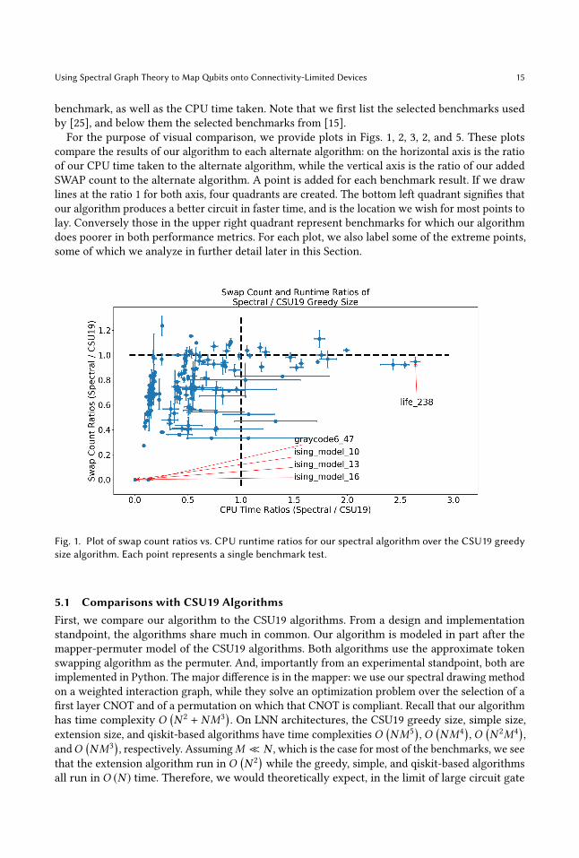
For the purpose of visual comparison, we provide plots in Figs. 1, 2, 3, 2, and 5. These plots

compare the results of our algorithm to each alternate algorithm: on the horizontal axis is the ratio

of our CPU time taken to the alternate algorithm, while the vertical axis is the ratio of our added

SWAP count to the alternate algorithm. A point is added for each benchmark result. If we draw

lines at the ratio 1 for both axis, four quadrants are created. The bottom left quadrant signifies that

our algorithm produces a better circuit in faster time, and is the location we wish for most points to

lay. Conversely those in the upper right quadrant represent benchmarks for which our algorithm

does poorer in both performance metrics. For each plot, we also label some of the extreme points,

some of which we analyze in further detail later in this Section.

Fig. 1. Plot of swap count ratios vs. CPU runtime ratios for our spectral algorithm over the CSU19 greedysize algorithm. Each point represents a single benchmark test.

5.1 Comparisons with CSU19 AlgorithmsFirst, we compare our algorithm to the CSU19 algorithms. From a design and implementation

standpoint, the algorithms share much in common. Our algorithm is modeled in part after the

mapper-permuter model of the CSU19 algorithms. Both algorithms use the approximate token

swapping algorithm as the permuter. And, importantly from an experimental standpoint, both are

implemented in Python. The major difference is in the mapper: we use our spectral drawing method

on a weighted interaction graph, while they solve an optimization problem over the selection of a

first layer CNOT and of a permutation on which that CNOT is compliant. Recall that our algorithm

has time complexity O(N 2 + NM3

). On LNN architectures, the CSU19 greedy size, simple size,

extension size, and qiskit-based algorithms have time complexities O(NM5

), O

(NM4

), O

(N 2M4

),

andO(NM3

), respectively. AssumingM ≪ N , which is the case for most of the benchmarks, we see

that the extension algorithm run in O(N 2

)while the greedy, simple, and qiskit-based algorithms

all run in O (N ) time. Therefore, we would theoretically expect, in the limit of large circuit gate

16 Lin, Anschuetz, and Harrow

Fig. 2. Plot of swap count ratios vs. CPU runtime ratios for our spectral algorithm over the CSU19 simplesize algorithm. Each point represents a single benchmark test.

Fig. 3. Plot of swap count ratios vs. CPU runtime ratios for our spectral algorithm over the CSU19 extensionsize algorithm. Each point represents a single benchmark test.

counts N , to have comparable runtimes with the extension algorithm while having slower runtimes

compared to the other three.

Looking at the results, we see that our algorithm performs better on both metrics for the

vast majority of benchmarks. Against the extension algorithm, our algorithm ran faster on all

benchmarks. Furthermore, our algorithm generated a smaller SWAP count graph in almost all

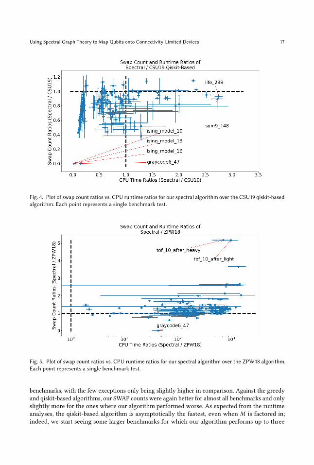
Using Spectral Graph Theory to MapQubits onto Connectivity-Limited Devices 17

Fig. 4. Plot of swap count ratios vs. CPU runtime ratios for our spectral algorithm over the CSU19 qiskit-basedalgorithm. Each point represents a single benchmark test.

Fig. 5. Plot of swap count ratios vs. CPU runtime ratios for our spectral algorithm over the ZPW18 algorithm.Each point represents a single benchmark test.

benchmarks, with the few exceptions only being slightly higher in comparison. Against the greedy

and qiskit-based algorithms, our SWAP counts were again better for almost all benchmarks and only

slightly more for the ones where our algorithm performed worse. As expected from the runtime

analyses, the qiskit-based algorithm is asymptotically the fastest, even when M is factored in;

indeed, we start seeing some larger benchmarks for which our algorithm performs up to three

18 Lin, Anschuetz, and Harrow

times as slowly. The greedy algorithm also has a better runtime N dependence compared to ours,

thus explaining the right trail of higher time ratios. Finally, our algorithm had the most mixed

performance against the simple size algorithm. While the majority of points still lay in the lower

left quadrant, our algorithm provided a circuit with more SWAPs in many more benchmarks.

Furthermore, our worst benchmarks resulted in SWAP counts over 1.6 times that of the simple size

algorithm.

Our overall conclusion is that our algorithm is quite competitive with the CSU19 algorithms. In

most cases, our algorithm finds circuits with significantly fewer SWAPs. This may be expected at

least in part due to our algorithm being more tailored towards LNN architectures through the use

of spectral drawing, while their algorithms target arbitrary connectivities. In terms of runtime, our

algorithm can be quite a bit faster for some smaller circuits, but in general is on the same order of

magnitude in terms of runtime. Theoretically, we do expect our algorithm to get slower for much

larger circuits; however, that limit is clearly not yet reached for circuits with up to 10,000 CNOTs.

Even above those counts, our algorithm still has polynomial asymptotic runtime.

5.2 Comparisons with ZPW18 AlgorithmNext, we compare our algorithm to the ZPW18 algorithm. Recall that the ZPW18 algorithm involves

an A* search across a state space involving all possible mappings. As there areM! possible mappings,

both worst-case runtime and storage complexities are O (M!). However, with A* search, the actual

runtime may be a lot less depending on the choice of heuristic; as a result, it is more difficult

to translate these theoretical runtime characteristics into experiments. Another difficulty in the

runtime comparisons has to do with implementation: the implementation of the ZPW18 algorithm

we compare against was written in C++. That means their code was compiled first before run on

the benchmarks, an advantage not afforded to either the CSU19 algorithm or ours.

When considering the results presented in Fig. 5, we immediately see their runtimes are many

orders of magnitude faster than ours. We believe that much of this is due to the difference in

implementation language (C++ vs. Python); however, without testing, this is merely speculation.

Our algorithm also only performs better on the SWAP count metric on aminority of the benchmarks;

additionally, with only one exception, the SWAP count decrease is only modest. In most cases, our

algorithm performs worse, hovering up to (and a few times beyond) 50% more SWAPs.

Because this algorithm is relatively exhaustive in nature and is also regarded as one of the best

performing algorithms for this problem, we find it encouraging that our algorithm does still find

smaller SWAP count circuits in a nontrivial number of benchmarks. Additionally, we believe that our

algorithm will scale better to larger circuits. In the benchmarks we tested, the qubit countM only

went as high as 16; therefore, the runtime limitations of the algorithm did not yet show. However,

asM increases, we do expect the O (M!) runtime to lead to the ZPW18 algorithm being infeasible.

One scalability issue that already did arise was with memory. In four of the benchmarks, their

algorithm ran out of memory. Again, with an O (M!) worst case scaling for the space complexity,

we would expect the memory needed to quickly rise to exorbitant levels. Indeed, this concern for

scalability was also raised by the authors of the SABRE algorithm [11].

5.3 Commentary on Specific BenchmarksWe close this Section with commentary on some of the outlier benchmarks marked in the fig-

ures. We start with the ising_model_10, ising_model_13, ising_model_16, and graycode6_47benchmarks. Each benchmark has the property that the circuit can be made LNN compliant with-

out any additional SWAPs. In fact, the circuits are already written in an LNN fashion. Therefore,

only a single mapping needs to be generated with no additional SWAPs. It can be seen that our

algorithm indeed detects the structure in all of these circuits and reports an optimal, zero SWAP

Using Spectral Graph Theory to MapQubits onto Connectivity-Limited Devices 19

compliant circuit. This is not necessarily the case for any of the alternate algorithms, especially for

graycode6_47.Many benchmarks on the far right of the figures, like life_238, sym9_148, and rd84_253 are

among the largest circuits we consider in terms of gate count. As expected, the larger the N , the

slower our algorithm becomes relative to those alternate algorithms.

One of our worst performing benchmark is 4mod5-bdd_287. The circuit itself is not that large(only 7 qubits and 31 CNOTs). However, the circuit properties do raise a weakness of our algorithm

in its current form. After the first two gates are applied, two of the seven qubits are never operated

on again. Rather than limiting ourselves to a five qubit subset of the LNN architecture, however, our

mapper continues trying to map all seven qubits. This likely leads to the two unused qubits being

disruptively placed in the middle of the circuit and moved around between mappings, rather than

staying fixed on the end. Additionally, the CNOTs are all such that no CNOTs can be commutated

past each other. This means the front layer is only a single CNOT. The fact that only one CNOT is

eligible at a time could mean the number of iterations is quite high and could also mean increased

reliance on the forced pairs fallback. All of these factors could explain why our algorithm takes an

unusually long time on this benchmark yet still produces a relatively high SWAP count circuit.

Finally, tof_10_after_heavy and tof_10_after_light are two benchmarks with which the

ZPW18 algorithm seems to vastly outperform the other algorithms. While the specific cause still

requires more investigation, it can likely be attributed to the ZPW18 algorithm’s ability to detect

the “staircase” pattern of CNOTs in the two benchmarks.

6 CONCLUSIONS6.1 Summary and SignificanceWe explored the use of spectral graph theory and drawing to map logical qubits to physical qubits

in connectivity-constrained devices. Concerned with the problem of transforming logical circuits

into connectivity-compliant ones, we first characterized the properties and strengths of many other

modern algorithms and decided to follow a mapper-permuter model. We focused our exploration

on linear nearest neighbor connectivities, and in particular explored how spectral drawing could

be used as part of the mapper. We contributed a novel way of generating a more sophisticated

weighted interaction graph based on the previously generated mapping and on layering properties

of the unapplied CNOTs. Having presented a class of algorithms with several configuration options,

we selected a set of ten options found to provide the best coverage across realistic benchmarks.

The overall meta-algorithm then generated ten circuits using these different options and returning

the best one. Finally, we compared our implementation to two recent, high-performing algorithms.

We find our implementation to be quite promising, constructing circuits with smaller SWAP counts

on many benchmarks while still having scalable space and runtime characteristics.

6.2 Future DirectionsThere are many future directions for this work. Some categories include:

(1) optimizing the current LNN algorithm,

(2) adapting the algorithm for other architectures and objective functions,

(3) making use of the spectral mapper in conjunction with other algorithms, and

(4) making use of other approximation or relaxation methods.

There are many minor optimizations that can be made on the current algorithm to improve

performance. As mentioned in Sec. 5.3, our algorithm does not properly detect when qubits go

unused part way through iterations. One solution is to detect when this occurs and fix the unused

qubits at the ends; then, continue the algorithm on just a subset of the physical qubits. More generally,

20 Lin, Anschuetz, and Harrow

further exploration of some common circuit patterns can help illuminate issues in our solver and

allow us to optimize for them. Another improvement is to further optimize the interaction graph

generation. To start off, a more exhaustive and systematic search over the parameters, (including

some that were fixed, like τ ), may find more optimal parameters and also might elucidate why

some parameters perform better than others.

We can also consider exploring variations of the connectivity-compliance problem. One obvious

modification is to consider more general connectivities. Because our algorithm relies on spectral

drawing, which involves mapping to coordinate locations and then to discrete locations, adapting to

general connectivities would be quite challenging. However, a two-dimensional, nearest neighbors

grid connectivity could be within the realm of possibility. Then, our algorithm would use not only

the Fiedler vector, but also the eigenvector with the next smallest eigenvalue. These vectors then

provide a coordinate location in 2D for each qubit. The question of mapping the coordinates to

discrete grid locations is not as straightforward, as there is not a strict ordering of 2D coordinates.

Even supposing a similar assignment strategy as in the 1D case were use, issues still arise related

to a fallback strategy. It is nontrivial to decide how to place forced pairs: which orientation they

are in, or which qubits to “shift aside” to make space. Additionally, when the number of physical

qubits exceeds that of the logical qubits, it is nontrivial to decide which physical qubits go unused.

All-in-all, the adaptation from LNN to a 2D grid still has many open questions. A more feasible

modification to consider is a change in the objective. So far, we have focused on circuit size, via

minimizing added SWAPs. However, another metric we can explore is minimizing circuit depth.

This would require no change to the current algorithm initially and would involve measuring the

circuit depth for the generated connectivity-complaint benchmark circuits.

Third, we propose that ideas from our spectral mapper may be used in conjunction with other

developed algorithms. Most straightforward is the inclusion of our spectral mapper as a mapper

option in the CSU19 mapper-permuter algorithm framework, albeit only for LNN connectivities.

There is also an opportunity to use our spectral mapper to provide an initial mapping. Many

search-style algorithms, like the ZPW18 A* algorithm [25] and SABRE [11], need to be seeded with

a good initial permutation; we suggest that our spectral mapper could be used for that purpose.

Finally, another direction we wish to explore is the search for different solving strategies. In

this work, we proposed the use of spectral graph theory, a framework that was not previously

explored for this problem. The motivation was that the spectral optimization problem provides a

relaxation of the original problem, which is to determine a list of the best mappings. While the

original problem cannot be exactly solved efficiently, the relaxed problem can. Right now, however,

the relaxation is done mapping-by-mapping: though it has lookahead properties and considers the

previous mapping, the optimization is still very much a local one. We leave as an open problem

the search for another optimization problem or framework that is efficient to exactly solve and

provides a global relaxation. The desire would be to frame the problem in such a way that a singleproblem can be solved, for all layers of CNOTs, and then the resulting relaxed solution can be

translated (e.g. rounded, assigned to discrete locations) to provide a strong approximate solution to

the original problem.

ACKNOWLEDGMENTSJXL was funded in part by NSF grant CCF-1729369. ERA was partially supported by a Lester Wolfe

Fellowship and the Henry W. Kendall Fellowship Fund from M.I.T. AWH was funded by NSF grants

CCF-1452616, CCF-1729369, PHY-1818914, ARO contract W911NF-17-1-0433 and the MIT-IBM

Watson AI Lab under the project Machine Learning in Hilbert space.

Using Spectral Graph Theory to MapQubits onto Connectivity-Limited Devices 21

REFERENCES[1] A. Chakrabarti, S. Sur-Kolay, and A. Chaudhury. Linear nearest neighbor synthesis of reversible circuits by graph

partitioning, 2011, arXiv:1112.0564.[2] D. Cheung, D. Maslov, and S. Severini. Translation techniques between quantum circuit architectures. In Workshop on

Quantum Information Processing, 2007.[3] A. M. Childs, E. Schoute, and C. M. Unsal. Circuit transformations for quantum architectures, 2019, arXiv:1902.09102.[4] A. Cowtan, S. Dilkes, R. Duncan, A. Krajenbrink, W. Simmons, and S. Sivarajah. On the qubit routing problem, 2019,

arXiv:1902.08091.[5] E. Farhi, J. Goldstone, and S. Gutmann. A quantum approximate optimization algorithm, 2014, arXiv:1411.4028.[6] W. Finigan, M. Cubeddu, T. Lively, J. Flick, and P. Narang. Qubit allocation for noisy intermediate-scale quantum

computers, 2018, arXiv:1810.08291.[7] L. K. Grover. Quantum mechanics helps in searching for a needle in a haystack. Physical review letters, 79(2):325, 1997.[8] J. P. i Silvestre and J. G. Salgado. Approximation heuristics and benchmarkings for the minla problem. In Alex,

volume 98. Citeseer, 1998.

[9] M. Juvan and B. Mohar. Optimal linear labelings and eigenvalues of graphs. Discrete Applied Mathematics, 36(2):153–168,1992.

[10] Y. Koren. On spectral graph drawing. In International Computing and Combinatorics Conference, pages 496–508.Springer, 2003.

[11] G. Li, Y. Ding, and Y. Xie. Tackling the qubit mapping problem for NISQ-era quantum devices. In Proceedings of theTwenty-Fourth International Conference on Architectural Support for Programming Languages and Operating Systems,pages 1001–1014. ACM, 2019.

[12] D. Maslov, S. M. Falconer, and M. Mosca. Quantum circuit placement. IEEE Transactions on Computer-Aided Design ofIntegrated Circuits and Systems, 27(4):752–763, 2008.

[13] T. Miltzow, L. Narins, Y. Okamoto, G. Rote, A. Thomas, and T. Uno. Approximation and hardness for token swapping,

2016, arXiv:1602.05150.[14] P. Murali, J. M. Baker, A. J. Abhari, F. T. Chong, and M. Martonosi. Noise-adaptive compiler mappings for noisy

intermediate-scale quantum computers, 2019, arXiv:1901.11054.[15] Y. Nam, N. J. Ross, Y. Su, A. M. Childs, and D. Maslov. Automated optimization of large quantum circuits with

continuous parameters. npj Quantum Information, 4(1):23, 2018, arXiv:1710.07345.[16] J. Olson, Y. Cao, J. Romero, P. Johnson, P.-L. Dallaire-Demers, N. Sawaya, P. Narang, I. Kivlichan, M. Wasielewski, and

A. Aspuru-Guzik. Quantum information and computation for chemistry, 2017, arXiv:1706.05413.[17] V. Y. Pan and Z. Q. Chen. The complexity of the matrix eigenproblem. In Proceedings of the thirty-first annual ACM

symposium on Theory of computing, pages 507–516. ACM, 1999.

[18] M. Pedram and A. Shafaei. Layout optimization for quantum circuits with linear nearest neighbor architectures. IEEECircuits and Systems Magazine, 16(2):62–74, 2016.

[19] J. Petit. Experiments on the minimum linear arrangement problem. Journal of Experimental Algorithmics (JEA), 8:2–3,2003.

[20] A. Shafaei, M. Saeedi, and M. Pedram. Optimization of quantum circuits for interaction distance in linear nearest

neighbor architectures. In Proceedings of the 50th Annual Design Automation Conference, page 41. ACM, 2013.

[21] P. W. Shor. Polynomial-time algorithms for prime factorization and discrete logarithms on a quantum computer. SIAMreview, 41(2):303–332, 1999.

[22] M. Y. Siraichi, V. F. d. Santos, S. Collange, and F. M. Q. Pereira. Qubit allocation. In Proceedings of the 2018 InternationalSymposium on Code Generation and Optimization, pages 113–125. ACM, 2018.

[23] R. Wille, D. Große, L. Teuber, G. W. Dueck, and R. Drechsler. RevLib: An online resource for reversible functions and

reversible circuits. In Int’l Symp. onMulti-Valued Logic, pages 220–225, 2008. RevLib is available at http://www.revlib.org.

[24] R. Wille, A. Lye, and R. Drechsler. Optimal swap gate insertion for nearest neighbor quantum circuits. In 2014 19thAsia and South Pacific Design Automation Conference (ASP-DAC), pages 489–494. IEEE, 2014.

[25] A. Zulehner, A. Paler, and R. Wille. An efficient methodology for mapping quantum circuits to the IBMQX architectures.

IEEE Transactions on Computer-Aided Design of Integrated Circuits and Systems, 2018.

22 Lin, Anschuetz, and Harrow

A SPECTRAL GRAPH THEORY PROOFSIn this section we include proofs of the claims made in Section 2.3.1. They are not original to our

paper (see e.g. [10]) but are included here for convenience.

Proof of Lemma 2.2. With use of the fact thatwi j = w ji and Li j = Lji , we see that:

xTLx =n∑i=1

n∑j=1

xix jLi j (16)

=

n∑i=1

x2i Lii + 2∑i<j

xix jLi j (17)

=

n∑i=1

∑k,i

x2iwik − 2

∑i<j

xix jwi j (18)

=∑i<k

x2iwik +∑k<i

x2iwik − 2

∑i<j

xix jwi j (19)

=∑i<j

x2iwi j +∑i<j

x2jw ji −∑i<j

2xix jwi j (20)

=∑i<j

wi j

(x2i − 2xix j + x

2

j

)(21)

=∑i<j

wi j(xi − x j

)2

(22)

as desired. □

Proof of lemma 2.3.

(L1n)i =n∑j=1

Li j (23)

=∑i,j

Li j + Lii (24)

=∑i,j

−wi j +∑k,i

wik (25)

= 0. (26)

□

B APPROXIMATE TOKEN SWAPPING ALGORITHMIn this section, we outline an approximate token swapping algorithm as proposed in [13]. First, we

define two operations. An unhappy swap occurs when we perform a swap for which one token was

already on its desired vertex and the other token is swapped closer to its desired vertex. A happyswap chain occurs when, given a path of l + 1 distinct vertices vi1 , . . . ,vil+1 , we perform in order

the l swaps(vi1 ,vi2

),(vi2 ,vi3

), . . . ,

(vil ,vil+1

)and every swapped token along the path is moved

strictly closer to its target vertex.

It turns out that as long as some token is not at its desired vertex, one of the above operations

exists. The approximate algorithm, then, involves finding either an unhappy swap or a happy swapchain and performing that operation. Furthermore, it was shown by [13] that this algorithm is

guaranteed to converge.

To efficiently detect one of the two valid operations, a companion graph F is created at each step.

First, F is given the same set of vertices V . For an edge between vertices v andw of the original

graph G, consider a swap along that edge. If this causes the token currently on vertex v to move

closer to its desired vertex, then a directed edge is added from v tow in F . A vertex with out-degree

0 represents a token at its desired location, and therefore any edge going into that vertex represents

an unhappy swap. Additionally, any directed cycle represents a happy swap chain. Therefore, if we

start at any vertex whose token is misplaced and travel along a directed path, we will eventually

end at a vertex with no outward vertices (thus detecting an unhappy swap) or return to a vertex

already in the path (thus detecting an unhappy swap chain). This algorithm ultimately runs in time

polynomial in the size of G, i.e. polynomial in |V | and |E |.

C RAW DATAIn this section, we present the full results of our benchmarking experiments, described in Sec. 5.

They appear in Table 2, across the next several pages.

Table 2. Results of benchmarking experiments on LNN architectures. Each row is a single benchmark, whereits name is the filename of the test circuit. Each benchmark is characterized in part by the number of qubitsand number of CNOTs in the original circuit. The algorithms we compare are our spectral mapper, the foursize mappers from CSU19 [3], and ZPW18 algorithm [25]. We run each algorithm, and characterize theperformance both by the number of added SWAPs in the connectivity-compliant circuit, and the amount ofCPU time taken. Note the benchmarks are ordered by the number of CNOTs in their circuit.

Original Circuit Spectral CSU19 (Greedy) CSU19 (Simple) CSU19 (Extend) CSU19 (Qiskit) ZPW18 (A*)

Benchmark Circuit Qubits CNOTs SWAP

Count

CPU Time

(sec)

SWAP

Count

CPU Time

(sec)

SWAP

Count

CPU Time

(sec)

SWAP

Count

CPU Time

(sec)

SWAP

Count

CPU Time

(sec)

SWAP

Count

CPU Time

(sec)

ex1_226 6 5 5 0.3 5 0.9 7 1.6 6 1.5 6.4 0.9 3 0.002

graycode6_47 6 5 0 0.09 4 0.7 6 1 5 0.9 4.2 0.6 1 0.002

xor5_254 6 5 5 0.3 5 0.8 7 1.6 6 1.6 6 0.8 3 0.003

ex-1_166 3 9 3 0.1 7 1.5 7 2.2 6 2 6.4 1.2 3 0.004

4gt11_84 5 9 3 0.2 11 1.8 8 2.1 6 2 6.4 1.2 5 0.002

4mod5-v0_20 5 10 5.4 0.3 8.4 1.3 8.6 2.1 8.4 1.9 9.2 1.3 4 0.005

ham3_102 3 11 3 0.1 7 1.4 6 2.2 5 2 7 1.4 4 0.005

4mod5-v1_22 5 11 6.2 0.3 9 1.4 8.2 2.3 8.8 2.3 10 1.5 5 0.002

mod5d1_63 5 13 8 0.3 8.2 1.5 11.6 2.9 11 2.3 10 1.5 8 0.003

4gt11_83 5 14 6 0.2 8 1.4 9 2.8 10 2.6 10 1.6 6 0.005

rd32-v0_66 4 16 8 0.3 11 2.1 8 3.1 8 3.1 10.8 2 7 0.004

rd32-v1_68 4 16 8 0.3 11 2.1 8 3.1 8 3.2 9.8 1.8 7 0.003

4mod5-v0_19 5 16 13.6 0.6 11 2.2 12 3.8 11 3.7 12.6 2.2 8 0.005

4mod5-v1_24 5 16 11 0.5 16 2.5 13 4 11 3.6 13.6 2.3 7 0.004

mod5mils_65 5 16 11.6 0.6 12 2.2 14 4.1 12 3.7 15.8 2.5 7 0.004

3_17_13 3 17 6 0.2 9 2.2 11 4 11 3.9 10 2 6 0.003

alu-v0_27 5 17 11 0.4 15.8 2.4 18 4.7 15 12.5 14.8 2.3 11 0.003

alu-v1_29 5 17 11 0.4 16.6 2.5 16.8 4.4 14.4 12.2 12.8 2 11 0.004

alu-v2_33 5 17 12.6 0.5 16 2.5 16 4.3 13 11.9 11.8 1.9 7 0.006

4gt11_82 5 18 7 0.3 13 1.9 10 3.1 14 3.3 14.4 2.1 8 0.004

alu-v1_28 5 18 13 0.4 17 2.6 18 4.7 14.8 12.3 13.6 2.2 11 0.005

alu-v3_35 5 18 11 0.4 16.6 2.5 15.6 4.2 15 12.4 15.6 2.4 11 0.004

alu-v4_37 5 18 11 0.4 16.6 2.5 18 4.7 15 12.6 14.2 2.2 11 0.006

decod24-v2_43 4 22 11 0.4 15 3 16 5.8 13 4.8 15.8 3 12 0.005

miller_11 3 23 9 0.4 17 3.5 15 5.1 14 4.7 14.2 2.6 9 0.004

decod24-v0_38 4 23 10 0.4 21 3.5 14 5 15 4.7 14.4 2.8 9 0.004

alu-v3_34 5 24 15 0.5 18 3.7 17.2 5.7 18 17.6 19.6 3.3 13 0.003

mod5d2_64 5 25 19.8 0.7 20 3.8 20 5.4 21 5.6 22.2 3.5 17 0.005

4gt13-v1_93 5 30 16 0.6 30.6 4.4 26 6.5 26.4 14.5 24.2 3.7 16 0.004

4gt13_92 5 30 17 0.6 31.4 4.3 27 6.7 27.4 21.4 27.8 4.1 19 0.007

4mod5-v0_18 5 31 19 0.8 22 4 24 7.3 20 6.4 24.6 4.1 15 0.005

4mod5-bdd_287 7 31 22 2.7 27 4.1 28 7.4 28 7.3 32.2 4.7 15 0.006

4mod5-v1_23 5 32 22.6 0.9 27 5.1 25 8.2 22 14.8 25.2 4.4 18 0.005

one-two-three-v2_100 5 32 16 0.6 26.6 4.2 30.6 7.5 31.2 13.8 28.2 4.2 18 0.004

one-two-three-v3_101 5 32 16 0.7 28.8 4.5 26.8 7.8 28.2 14 26.4 4 20 0.005

decod24-bdd_294 6 32 18 2 25 4.8 22 6.5 17 5.3 23.6 4 16 0.005

rd32_270 5 36 21 0.9 34 5.4 22 7.5 28.6 16.8 29.4 4.8 19 0.006

4gt5_75 5 38 23 0.7 32 5.1 27.6 8.7 25.4 28.8 29 4.6 22 0.005

alu-v0_26 5 38 22 0.7 29 5.4 38 9.6 30 7.8 37 5.4 25 0.004

decod24-v1_41 5 38 25.6 1 38.2 5.5 30 8.1 26.8 14.3 29.6 4.7 23 0.005

alu-bdd_288 7 38 31 2.9 42.8 5.3 34.6 8 43.2 14.5 39 5.4 25 0.005

4gt5_76 5 46 25 0.7 46 6.1 38 10.7 37 18.1 43.4 6 25 0.006

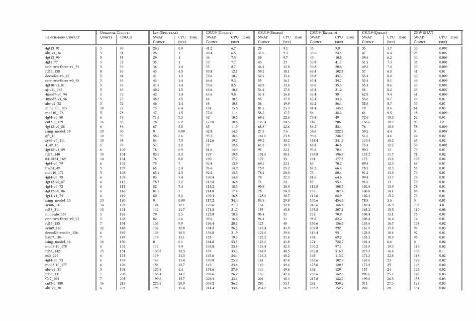
Original Circuit Lin (Spectral) CSU19 (Greedy) CSU19 (Simple) CSU19 (Extend) CSU19 (Qiskit) ZPW18 (A*)

Benchmark Circuit Qubits CNOTs SWAP

Count

CPU Time

(sec)

SWAP

Count

CPU Time

(sec)

SWAP

Count

CPU Time

(sec)

SWAP

Count

CPU Time

(sec)

SWAP

Count

CPU Time

(sec)

SWAP

Count

CPU Time

(sec)

4gt13_91 5 49 26.8 0.9 41.2 6.7 28 9.1 36 9.8 35 5.7 30 0.007

alu-v4_36 5 51 28 1 40.4 6.5 31.6 9.3 33.6 24.5 41 6.4 25 0.007

4gt13_90 5 53 29 1 46 7.3 30 9.7 40 10.5 39.6 6.2 34 0.006

4gt5_77 5 58 35 1 50 7.7 43 13 50.8 41.7 51.2 7.3 36 0.008

one-two-three-v1_99 5 59 36 1.4 55 8.7 46.4 12.8 50.8 20.6 49.2 7.4 35 0.009

rd53_138 8 60 43 4.5 80.8 12.1 59.2 18.1 66.4 102.8 57 6.5 41 0.01

decod24-v3_45 5 64 41 1.3 78.6 10.7 52.2 15.6 56.8 43.3 55.4 8.2 40 0.009

one-two-three-v0_98 5 65 43 1.4 66.6 9.3 55 16.1 60.4 34.7 53.4 8.1 44 0.009

4gt10-v1_81 5 66 41.8 1.4 53.6 8.5 42.8 13.6 43.6 35.3 55.4 8.6 40 0.007

aj-e11_165 5 69 40.2 1.5 63.6 10.6 54.4 17.3 43.8 21.2 54 8.2 33 0.007

4mod7-v0_94 5 72 42 1.4 67.6 9.8 51.4 16.8 52.4 38 62.8 9.4 41 0.006

4mod7-v1_96 5 72 48.6 1.5 64 10.5 55 17.9 62.4 34.2 53.6 8.7 44 0.01

alu-v2_32 5 72 46 1.4 68 10.8 56 19.9 64.2 56.4 55.6 8.7 50 0.01

mini_alu_305 10 77 75 6.4 101 15.6 81.2 25.3 81.4 145.6 79 8.6 61 0.03

mod10_176 5 78 47 1.5 77.6 11.4 58.2 17.7 56 38.2 64 9.5 48 0.009

4gt4-v0_80 6 79 71.6 5.5 62 10.5 69.4 22.6 79.8 49 72.6 10.3 52 0.01

cnt3-5_179 16 85 78 6.2 172.8 18.6 125.4 24.5 147 206 156.6 10.2 93 1.2

4gt12-v0_88 6 86 67 5.8 65 11.3 68.8 22.6 86.2 55.4 76 10.6 58 0.009

ising_model_10 10 90 0 0.08 42.8 14.8 27.8 7.6 54.6 222.7 50.2 4.4 0 0.009

qft_10 10 90 58.2 2.6 93.2 18.4 161.6 23.8 93.6 246.5 51.6 4.6 44 0.02

sys6-v0_111 10 98 84 7.3 112.6 19.2 99.2 30.2 158.4 241.9 110.4 10.2 65 0.02

4_49_16 5 99 57 2.2 78 12.6 61.8 19.5 68.8 46.6 75.4 12.2 59 0.008

4gt12-v1_89 6 100 78 6.9 81.6 14.3 95 22.1 90.6 70.4 90.2 13 70 0.01

rd73_140 10 104 83.6 8.3 129 19.8 101.6 30.1 149.8 196.8 118.2 11.7 71 0.02

0410184_169 14 104 76 8.8 190 17.7 179 33 161 177.8 173 13.6 105 0.04

4gt4-v0_79 6 105 75 7 92.4 13.9 69.2 22.1 83 70.2 89.4 12.5 68 0.01

hwb4_49 5 107 65 2.4 96.6 14.9 75.8 25.2 87.2 66.4 78.2 12.3 56 0.01

mod10_171 5 108 65.4 2.3 92.2 15.5 78.2 28.3 75 60.4 91.2 13.3 70 0.01

4gt4-v0_78 6 109 83 7.4 100.4 14.8 78 22.3 81.6 64.6 99.4 13.7 74 0.01

4gt12-v0_87 6 112 78.8 7.2 112.8 16.8 74 24 89 95.4 94.6 13 79 0.01

4gt4-v0_72 6 113 82 7.4 113.2 18.5 90.8 28.9 112.8 108.5 102.8 13.9 78 0.01

4gt12-v0_86 6 116 81.8 7 114.8 17.4 78 24.9 102 107.4 106.8 14.1 86 0.01

4gt4-v1_74 6 119 80 8.2 109.4 16.8 128.6 30.7 112.6 68.9 102.4 15.2 76 0.01

ising_model_13 13 120 0 0.09 117.2 34.4 84.8 29.8 105.6 454.6 78.8 5.6 0 0.01

sym6_316 14 123 124 12.1 170.6 21.3 154 32.8 216.6 166.8 182.4 16.9 138 4.8

rd53_311 13 124 112 11.7 171.8 21.7 155 45.8 193.8 207.1 165.2 15.5 119 0.08

mini-alu_167 5 126 79 2.5 123.8 18.8 96.4 31 102 70.9 104.4 15.1 76 0.01

one-two-three-v0_97 5 128 82 2.6 99.6 16.6 94.4 31 98.6 82.2 108.4 16.4 74 0.01

rd53_135 7 134 136 9.9 136.4 20.1 125 40 150.6 156.7 133.6 16.7 108 0.02

sym9_146 12 148 132 12.8 194.2 26.5 143.4 41.9 239.8 292 167.8 15.8 99 0.03

decod24-enable_126 6 149 134 10.5 136.8 21.9 121.6 39.4 116.4 95 128.8 18.6 97 0.01

ham7_104 7 149 119 11.1 133 19.3 123.2 31.6 144 69.2 135.2 18.9 96 0.01

ising_model_16 16 150 0 0.1 164.8 53.5 123.6 41.8 174 722.7 101.4 6.6 0 0.02

mod8-10_178 6 152 117 9.9 138.8 23.6 118.4 42.5 150.2 97.1 131.8 19.3 113 0.02

rd84_142 15 154 130.8 13.3 197 33.3 161.8 48.5 262.8 516.8 215.2 16.4 109 0.1

ex3_229 6 175 119 11.3 147.6 24.4 116.2 40.2 143 113.2 171.2 22.8 118 0.02

4gt4-v0_73 6 179 145 11.4 170.8 25.9 141 47.4 168.6 102.9 162.6 23 129 0.02

mod8-10_177 6 196 156 13.7 142 23.6 149 49.4 175.6 120.3 172.8 25 146 0.02

alu-v2_31 5 198 127.8 4.4 174.6 27.9 144 49.6 144 129 157 24 125 0.02

rd53_131 7 200 156.4 14.7 209.6 26.2 155 42.6 230.6 162.3 205.6 25.7 146 0.03

C17_204 7 205 199.6 15.7 226.4 33.1 201 48.4 217.6 182.2 199.6 26.3 153 0.03

cnt3-5_180 16 215 225.8 20.9 309.2 36.7 280 55.1 292 359.2 311 27.5 127 0.03

alu-v2_30 6 223 195 15.4 214.4 33.4 234.2 56.9 193.2 152.7 202 28 154 0.02

Original Circuit Lin (Spectral) CSU19 (Greedy) CSU19 (Simple) CSU19 (Extend) CSU19 (Qiskit) ZPW18 (A*)

Benchmark Circuit Qubits CNOTs SWAP

Count

CPU Time

(sec)

SWAP

Count

CPU Time

(sec)

SWAP

Count

CPU Time

(sec)

SWAP

Count

CPU Time

(sec)

SWAP

Count

CPU Time

(sec)

SWAP

Count

CPU Time

(sec)

mod5adder_127 6 239 214.8 16.7 220.8 35.7 196.8 64.8 228.6 160.8 220.6 30.2 169 0.03

qft_16 16 240 153 7.5 333.6 77.7 845.8 86 307 1056.4 142.2 9.9 119 0.9

rd53_133 7 256 171.4 18.9 303.4 35.2 267.6 48.8 265.2 216.1 263.6 32.9 180 0.03

majority_239 7 267 220.2 20.9 249.6 37.1 251.6 68.4 308.2 222.2 261.2 33.9 197 0.04

ex2_227 7 275 228.8 22.2 274.6 40.1 197 56 288.8 212.4 272.2 35 193 0.03

cm82a_208 8 283 253 24.7 265.6 40.8 198.8 59.7 285.8 230.8 294.4 36.1 202 0.03

sf_274 6 336 277 26.3 275.4 45.6 243.8 81.3 310.2 145.6 284 42.2 239 0.04

sf_276 6 336 293 25.1 289.2 47 273 77.6 272.8 200.9 299.8 42.9 250 0.03

con1_216 9 415 452.4 39.1 478.6 60.7 463.2 105.7 442.6 355.9 463.2 54.3 365 0.05

wim_266 11 427 430.6 43.5 402.2 58.2 421.4 95.2 563.2 377.5 467 53.7 336 0.05

rd53_130 7 448 405.2 37.4 455.2 68.2 382.4 109.8 492.8 372.4 459.2 57.6 338 0.06

f2_232 8 525 454 48.7 559.6 72.3 444.4 108.4 551.6 392.2 545.8 68.7 398 0.09

cm152a_212 12 532 421 57.2 570.2 74.3 377.2 119.6 672.6 399.6 567.4 70.3 417 0.07

rd53_251 8 564 542 54.4 563 78.8 470.8 122.7 604 398.3 541.4 69.5 429 0.07

hwb5_53 6 598 513 50 518.8 81.6 520.4 157.8 528.4 407.9 543 76 417 0.06

cm42a_207 14 771 731 92.1 658.4 102 606.8 155.4 895.6 597.3 866.8 100.5 608 0.1

pm1_249 14 771 731 91.8 664 101.8 628 161.9 917.8 595.5 844.8 98.9 608 0.1

dc1_220 11 833 830.4 92.7 803.2 107.4 711.4 187.2 1096 629.9 904.8 107.3 678 0.1

squar5_261 13 869 987.2 103.3 1088 120.7 1088.4 206.6 1173.8 776.1 1090.2 115 763 0.2

sqrt8_260 12 1314 1886.6 172.6 1745.6 194.2 1519.2 321.1 1925.6 1190.5 1735 181.4 1223 1.2

z4_268 11 1343 1503 168.5 1594.6 199.8 1226.4 301.7 1839.6 1401.4 1587.4 176.2 1153 0.9

radd_250 13 1405 1552 190.1 1767.8 202.1 1203.4 308.1 1941.2 1155.6 1715.6 190.2 1185 9.1

adr4_197 13 1498 1775 205.5 1791.4 209.5 1647.2 397 2050 1370.9 1875.8 197.7 1370 0.3

sym6_145 7 1701 1483.4 198.1 1618.2 238.9 1729.6 462.7 1803.8 1263.7 1668.8 220.7 1215 0.2

misex1_241 15 2100 2235.4 325.3 2182.6 264.2 2289.8 427.2 2658.6 1293.4 2508.6 282.7 1749 0.3

rd73_252 10 2319 2812 348.9 2706.4 329.9 1958.4 497.6 3101.6 2049.3 2793.2 309.1 1995 14.4

cycle10_2_110 12 2648 3155.4 440.7 3479.6 369.1 2834 608.7 3552.6 1998.3 3342.4 356.1 2414 1.6

hwb6_56 7 2952 2850.8 455.2 2862.4 420.5 2665.6 773.5 3036.6 2290.7 2910.6 366.9 2140 0.4

square_root_7 15 3089 4826.6 580.8 4543 492.8 4478 1129.6 4936.4 3788.3 4228.6 417.8 3267 11.3

ham15_107 15 3858 4136.6 814.4 4597.6 534.8 4254 1015.5 4933.4 3138.1 4572.4 511.9 3308 2.4

dc2_222 15 4131 5193.6 914.1 5558 583.4 4942.4 955.6 5640.8 3183.9 5485.4 563.8 3906 8.6

sqn_258 10 4459 5055.8 944 5139 643.8 4313.4 1043.2 5710.2 4252.4 5149.2 590.6 out of memory

inc_237 16 4636 5119.6 1101.5 5285.6 606.4 5723 1041.2 5746.6 3348.9 5678 617 out of memory

cm85a_209 14 4986 6066.6 1215.5 6411.8 706.1 6444.6 1247.8 6583.8 3630.7 6667.8 693 4658 14.3

rd84_253 12 5960 7825.2 1585.4 7813.8 902 5125.2 1323.5 8655.6 6197.3 7746.2 796.6 out of memory

root_255 13 7493 10226.8 2310.7 9827.4 1158.7 7694.2 1815.3 10710.4 8786.3 9988.6 993.2 out of memory

co14_215 15 7840 13259.4 2332.3 11722 1342.5 11691.8 2723.2 12480 14008.2 11559.4 1026.3 7704 78.9

mlp4_245 16 8232 10745.2 2863 11617 1178 10712.4 2070.9 11598.2 7132.3 11311.8 1136.6 out of memory

sym9_148 10 9408 8822 3328 9563.2 1308.2 9318.4 2715 11375.8 8304.2 9891.6 1219.7 out of memory

life_238 11 9800 11817.8 3741.9 12467.6 1416.4 12296.2 2607.2 13974.6 8893.9 12715.6 1359.1 out of memory

tof_3_after_heavy 5 14 8 0.2 21 0.9 10 0.7 12 0.8 9.2 0.5 4 0.001

tof_3_after_light 5 14 8 0.2 21 0.9 10 0.7 12 0.8 9.8 0.5 4 0.002

barenco_tof_3_after_heavy 5 18 11 0.3 14 0.8 10 0.7 12 0.9 13 0.7 8 0.002

barenco_tof_3_after_light 5 20 12 0.4 14 0.9 10 0.7 12 0.9 13 0.7 8 0.001

tof_4_after_heavy 7 22 11 1.7 33 1.5 22 1.3 25 1.6 28.8 1.3 6 0.004

tof_4_after_light 7 22 11 1.1 33 1.6 22 1.3 25 1.6 23.6 1.2 6 0.002

mod5_4_after_heavy 5 28 15.2 0.6 26 1.2 18 1.1 22 1.3 21.4 1 12 0.001

mod5_4_after_light 5 28 14.8 0.6 26 1.2 18 1.1 22 1.3 17.8 0.9 12 0.004

tof_5_after_heavy 9 30 20.8 2 51 2.6 37 2.1 39 3.8 43.8 2.1 8 0.003

tof_5_after_light 9 30 20.6 2 51 2.6 37 2.1 39 3.8 36.6 1.8 8 0.003

barenco_tof_4_after_heavy 7 34 34 2.7 41 1.9 24 1.6 26 1.9 33.8 1.6 16 0.004

barenco_tof_4_after_light 7 40 22 3 46.8 2.3 24 1.6 26 1.9 26.8 1.5 16 0.004

mod_mult_55_after_heavy 9 40 44 2.4 59.8 3.7 48.2 5.5 62.8 16.1 49.6 2.2 30 0.008

Original Circuit Lin (Spectral) CSU19 (Greedy) CSU19 (Simple) CSU19 (Extend) CSU19 (Qiskit) ZPW18 (A*)

Benchmark Circuit Qubits CNOTs SWAP

Count

CPU Time

(sec)

SWAP

Count

CPU Time

(sec)

SWAP

Count

CPU Time

(sec)

SWAP

Count

CPU Time

(sec)

SWAP

Count

CPU Time

(sec)

SWAP

Count

CPU Time

(sec)

mod_mult_55_after_light 9 40 44 3.5 60.6 3.7 46.6 5.3 66.4 15.8 61.2 2.5 30 0.007

barenco_tof_5_after_heavy 9 50 60.8 3.4 85 3.9 53 3.7 59 5.3 71 3.2 23 0.004

vbe_adder_3_after_heavy 10 50 30 3.6 55.4 4.7 60 5.6 76.4 24 58 2.8 33 0.02

vbe_adder_3_after_light 10 50 43 5 53.8 4.8 58.4 5.5 84.8 23.8 54 2.6 33 0.02

barenco_tof_5_after_light 9 60 46.6 4.7 89 4.4 55 3.8 64 6.7 63.4 3.1 23 0.003

csla_mux_3_after_heavy 15 70 86.4 5.2 180.2 15.9 158 19.6 142.2 205.5 125 5.9 108 0.2

tof_10_after_heavy 19 70 93.2 7.9 258 19 192 13.7 275 112.8 173 10.9 18 0.01

tof_10_after_light 19 70 93 8.1 258 19.1 192 13.7 275 111.1 169.2 10.6 18 0.008

rc_adder_6_after_heavy 14 71 75 7.3 173 14.4 156.6 24.9 139.4 139 145.4 6.3 83 0.05

rc_adder_6_after_light 14 73 75 6.6 183 15 156.8 24 158.4 127.8 160.2 6.7 83 0.05

csla_mux_3_after_light 15 76 95.8 5 168.6 14.8 147.8 21.7 146.4 194.8 136 6.3 out of memory

mod_red_21_after_heavy 11 77 106 5.3 114.2 7.1 128.6 9.2 129 30.8 105.6 5 59 0.008

mod_red_21_after_light 11 81 78 6.1 116 7.4 134 9.4 127.2 28.1 102.2 5.2 59 0.01

gf2ˆE4_mult_after_heavy 12 99 124.4 6.3 171.6 11.7 173 16.1 158.2 85.4 153.8 6.6 109 0.03

gf2ˆE4_mult_after_light 12 99 125 6 168.8 11.4 173.8 16.1 158 85.1 150.6 6.6 128 0.05

barenco_tof_10_after_heavy 19 130 212.2 17.1 382.2 27.6 333 33.1 350.8 93.4 334.6 19.4 58 0.01