Embed Size (px)
Citation preview

José RepondArgonne National Laboratory
Review of the Status of the RPC-DHCAL
SiD WorkshopSLAC, Stanford, California
October 14 – 16, 2013

2
This talk will
Review the status of the RPC-DHCAL
→ Emphasis on what we have learned → Emphasis on open questions
Outline
DHCAL: Quick recap Operational problems Simulation of response Calibration of RPC response Response/resolution Further R&D

J.Repond DHCAL
3
DHCAL Construction Fall 2008 – Spring 2011
Resistive Plate Chamber
Sprayed 700 glass sheets Over 200 RPCs assembled → Implemented gas and HV connections
Electronic Readout System
10,000 ASICs produced (FNAL) 350 Front-end boards produced
→ glued to pad-boards 35 Data Collectors built
6 Timing and Trigger Modules built
Assembly of Cassettes
54 cassettes assembledEach with 3 RPCs
and 9,216 readout channels
350,208 channel system in first test beam Event displays 10 minutes after closing enclosure
Extensive testing at every step

J.Repond DHCAL
4
Testing in BeamsFermilab MT6
October 2010 – November 2011 1 – 120 GeV Steel absorber (CALICE structure)
CERN PS
May 2012 1 – 10 GeV/c Tungsten absorber (structure provided by CERN)
CERN SPS
June, November 2012 10 – 300 GeV/c Tungsten absorber
Test Beam Muon events Secondary beam
Fermilab 9.4 M 14.3 M
CERN 4.9 M 22.1 M
TOTAL 14.3 M 36.4 M
A unique data sample
RPCs flown to GenevaAll survived transportation

5
Operational/design problems
Loss of efficiency on edges of RPCs
Due to slight increase in gap size Channels not perfectly molded Simple solution for future RPCs
Loss of HV contact
Glass sprayed with resistive ‘artist’ paint Surface resistivity 1 – 10 MΩ∕□ As time passed, order 20/150 RPCs lost HV In part compensated by raising HV (6100 → 6800 V) In future will use carbon film (was not available in 2008 – 10)

6
Simulation of the Muon Response
RPC_sim_ Spread functions Comment
3 R e-ar + (1-R) e-br To help the tail
4 e-ar Based on measurement by STAR
5 R e-(r/σ1)^2+ (1-R) e-(r/σ2)^2 Commonly used
6 1/(a + r2)3/2 Recently came across
Simulation procedure
Take location of each energy deposit in gas gap from GEANT4 Eliminate close-by avalanches within dcut
Generate charge according to measured distribution, adjust using Q0
Spread charge on anode pads using various spread functions Apply threshold T

7
Tuning of parameters
Choose ‘clean’ regions away from problems dcut parameter to be tuned later with electrons Difficult to tune simultaneously core and tail of distribution RPC_sim_5 my personal favorite But RPC_sim_3 only released for public consumption
RPC_sim_3 (2 exponentials)

8
Response in entire plane
Fishing lines simulated by GEANT4 Loss of efficiency at edges simulated with decrease of Q
RPC_sim_3 (2 exponentials)

9
Simulation of electrons
In principle only dcut parameter left to tune Different RPC_sim programs result in widely different
Response Shower shapes Hit density distributions
→ The simulation of the tail in the muon spectra is important
Simulation of pions
No additional parameters ‘Absolute’ prediction Uncertainties in muon simulation packed into systematic error
Back to simulating muons
Attempt to take ionization of particles (βγ) into account Attempt to take location of ionization in gas gap into account

J. Repond - The DHCAL
10
Calibration of the DHCAL
RPC performance
Efficiency to detect MIP ε ~ 95% Average pad multiplicity μ~ 1.5 Calibration factors C = εμ Equalize response to MIPS (muons)
Calibration for secondary beam
If more than 1 particle contributes to signal of a given pad → Pad will fire, even if efficiency is low → Full calibration will overcorrect
i
RPC
RPCi iicalibrated HH
n
0
00
Full calibration
Simulation
Correction for differences in efficiency/multiplicities between RPCs

J. Repond - The DHCAL
11
Density weighted calibration
Derived entirely based on Monte Carlo
Assumes correlation between
Density of hits ↔ Number of particles contributing to signal of a pad
Mimics different operating conditions with
Different thresholds
Utilizes fact that hits generated with the
Same GEANT4 file, but different operating conditions can be correlated
Defines density bin for each hit
Bin 0 – 0 neighbors, bin 1 – 1 neighbor …. Bin 8 – 8 neighbors
Weights each hit
To restore desired density distribution of hits
Warning:This is rather
COMPLICATED

J. Repond - The DHCAL
12
Example: 10 GeV pions: Correction from T=400→ T=800

J. Repond - The DHCAL
13
Expanding technique to large range of operating conditions
GEANT4 files
Positrons: 2, 4, 10, 16, 20, 25, 40, 80 GeV Pions: 2, 4, 8, 9.9 19.9 25, 39.9 79.9 GeV
Digitization with RPC_sim
Thresholds 0f 0.2, 0.4, 0.6, 0.8, 1.0
Calculate calibration factors
Use one sample as ‘data’ Correct to another sample used as ‘target’ Use all combinations of ‘data’ and ‘target’
Plot
For each density bin, plot C as function of R = (εTμT)/(εDμD) → Some scattering of the points
π: Density bin 3
R = (εTμT)/(εDμD)
25 GeV

π: Density bin 3
R = (εTμT)/(εDμD)
J. Repond - The DHCAL
14
Empirical function of εT, μT, εD, μD
Positrons
Pions
Different energies
Similar results → Assume CF energy independent
0.23.0
0.23.0
DD
TTeR
5.13.0
5.13.0
DD
TTR
R = (εTμT)0.3/(εDμD)1.5
π: Density bin 3
Calib
ratio
n fa
ctor
sCa
libra
tion
fact
ors
25 GeV

J. Repond - The DHCAL
15
Fits of CFs as function of R
pRC Power law
Pion fits
Positron fits
similar

J. Repond - The DHCAL
16
Calibrating different runs at same energy
Uncalibrated responseFull calibrationDensity – weighted calibrationHybrid calibration (density bins 0 and 1 receive full calibration)
4 GeV π+ 8 GeV e+

J. Repond - The DHCAL
17
Comparison of different calibration schemes χ2 of distribution of means for different runs at same energy
→ All three schemes improve the spread

J. Repond - The DHCAL
18
Linearity of pion response: fit to aEm
Uncalibrated response
4% saturation
Full calibration
Perfectly linear up to 60 GeV (in contradiction to MC predictions)
Density- weighted calibration/Hybrid calibration
1 – 2% saturation (in agreement with predictions)

J. Repond - The DHCAL
19
Resolution for pions
Calibration
Improves result somewhat
Monte Carlo prediction
Around 58%/√E with negligible constant term
Saturation at higher energies
→ Leveling off of resolution

20
Software compensation
Typical calorimeter
Unequal response to electrons and hadrons Hadronic showers contain varying fraction of photons → Degraded resolution for hadrons
Hardware compensation
Equalization of the electron and hadron response Careful tuning of scintillator and absorber thicknesses ZEUS calorimeter best example
Software compensation
Identification of electromagnetic subshowers Different weighting of em and hadronic shower deposits Significant improvement of hadronic resolution
Fe-AHCAL

21
Over- Compensation
Compensating the DHCAL
Response of the DHCAL
Em response is highly non-linear (saturating) Hadronic response is close to linear Response compensating around 8 GeV
Definition of hit density
Defined for each hit Hit density = number of close-neighbor hits in the same plane
Assumption
Hit density is related to local particle density
Linearize the em response
By weighting hits in each hit density bins
Check the hadronic response and resolution
Studies limited to simulation

22
Linearizing the EM Response – Fe-DHCAL
High weights for isolated hits
Low weights for medium density: mostly due to hit multiplicity ~ 1.6
Very high weight forhigh density bins:correction for saturation
Simulation of positron showers
Set 1: 2, 6, 10, 16, 25 GeV Set 2: 2, 6, 16 , 32, 60 GeV
Target response
14.74 hits/GeV (arbitrary) Weights calculated such that linearity is optimized

23
Positron Response after Weighting – Fe-DHCAL
(no weights)
(set 1 weights)
(set 2 weights)
Fits to power law
β=1 means linear
E
Results as expected
Linearity significantly improved Set 2 weights provide better results

24
Positron Resolution after Weighting – Fe-DHCAL
Results
Corrected for non-linearity effects (important!) Resolution calculated from full-range Gaussian fits (not good at low energy) Not much difference between set 1 and 2 Overall modest improvement (as expected)

25
Pion Response after Weighting – Fe-DHCAL
(no weights)
(set 1 weights)
(set 2 weights)
Fits to power law
β=1 means linear
E
Results
Un-weighted linearity much worse than in data → Due to differences in real and simulated avalanches in RPCs Leakage cut applied: no more than 10 hits in tail catcher

26
Pion Resolution after Weighting – Fe-DHCAL
Results
Pion linearity and resolution significantly improved At high energies, distributions become more symmetric → Example: 60 GeV pions

27
Software Compensation in Data – Fe-DHCAL
Results
Similar to simulation, but not quite as good (e/h closer to unity in data) A few issues to be sorted out, such as contamination in data sample Not yet approved for public consumption

28
Software Compensation in Simulation – W-DHCAL
Comparison with the Fe-DHCAL
e/h much smaller than for Fe-DHCAL → Expect larger improvement
Pion results
Linearity improved, but e/h still far from unity Resolution improved by 25 – 50% Distributions improved, but tail remains

29
Further R&D

30
1-glass RPCs
Offers many advantages
Pad multiplicity close to one → easier to calibrate Better position resolution → if smaller pads are desired Thinner → safes on cost Higher rate capability → roughly a factor of 2
Status
Built several large chambers Tests with cosmic rays very successful → chambers ran for months without problems Both efficiency and pad multiplicity look good
Efficiency Pad multiplicity
J. Repond - The DHCAL
31
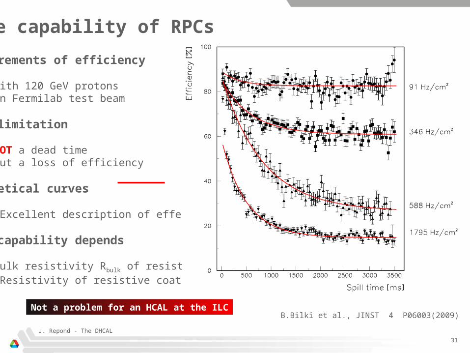
Rate capability of RPCs
Measurements of efficiency
With 120 GeV protons In Fermilab test beam
Rate limitation
NOT a dead time But a loss of efficiency
Theoretical curves
Excellent description of effect
Rate capability depends
Bulk resistivity Rbulk of resistive plates (Resistivity of resistive coat)
Not a problem for an HCAL at the ILCB.Bilki et al., JINST 4 P06003(2009)

J.Repond: DHCAL
32
High-rate Bakelite RPCsBakelite does not break like glass, is laminated but changes Rbulk with depending on humidity but needs to be coated with linseed oil
Gas inlet Gas outlet
Gas flowdirection
Fishing line
Sleeve aroundfishing line
Additional spacer
Use of low Rbulk Bakelite with Rbulk ~ 108 - 1010 and/or Bakelite with resistive layer close to gas gap
Several chambers built at ANL
Gas
Resistive layer for HV

J.Repond: DHCAL
33
High-rate Bakelite RPCsBakelite does not break like glass, is laminated but changes Rbulk with depending on humidity but needs to be coated with linseed oil
Gas inlet Gas outlet
Gas flowdirection
Fishing line
Sleeve aroundfishing line
Additional spacer
Use of low Rbulk Bakelite with Rbulk ~ 108 - 1010 and/or Bakelite with resistive layer close to gas gap
Several chambers built at ANL
Gas
Resistive layer for HV

Noise measurement: B01
1st run at 6.4 kV Last run, also 6.4kV, RPC rotated 900
Readout area
Fishing lines
(incorporated resistive layers)

J.Repond: DHCAL
35
Noise measurementsApplied additional insulationRate 1 – 10 Hz/cm2 (acceptable)Fishing lines clearly visibleSome hot channels (probably on readout board)No hot regions
Cosmic ray testsStack including DHCAL chambers for trackingEfficiency, multiplicity measured as function of HVHigh multiplicity due to Bakelite thickness (2 mm)

J.Repond: DHCAL
36Tests carried out by University of Michigan, USTC, Academia Sinica
GIF Setup at CERN

J.Repond: DHCAL
37
First results from GIF
Source on
Source off
Background rate
Absolute efficiency not yet determined
Clear drop seen with source on
Background rates not corrected for efficiency drop
Irradiation levels still to be determined (calculated)

J.Repond: DHCAL
38
Development of semi-conductive glass
Co-operation with COE college (Iowa) and University of Iowa
World leaders in glass studies and development
Development of Vanadium based glass (resistivity tunable)
First samples produced with very low resistivity Rbulk ~ 108 Ωcm
New glass plates with Rbulk ~ 1010 Ωcm in production
Glass to be manufactured industrially (not expensive)

39
High Voltage Distribution System
Generally
Any large scale imaging calorimeter will need to distribute power in a safe and cost-effective way
HV needs
RPCs need of the order of 6 – 7 kV
Specification of distribution system
Turn on/off individual channels Tune HV value within restricted range (few 100 V) Monitor voltage and current of each channel
Status
Iowa started development First test with RPCs encouraging Work stopped due to lack of funding Size of noise file
(trigger-less acquisition)

40
Gas Recycling SystemDHCAL’s preferred gas
Development of ‘Zero Pressure Containment’ System
Work done by University of Iowa/ANL
Status
First parts assembled…
Gas Fraction [%] Global warming potential (100 years, CO2 = 1)
Fraction * GWP
Freon R134a 94.5 1430 1351
Isobutan 5.0 3 0.15
SF6 0.5 22,800 114
Recycling mandatory for larger RPC systems

41
SummaryThe DHCAL
was successfully designed and built (2008 – 2010) was successfully tested at FNAL with Fe-absorber plates (2010 – 2011) was successfully tested at CERN with W- absorber plates (2012)
had few design/operational issues (HV contact, gas gap thickness)
taught us a lot about digital calorimetry (simulation, calibration, software compensation)
Open issues
optimization (chamber design, pad size ← requires tuning of PFAs) mechanical integration power distribution (common to all technologies) gas recirculation high-rate capability (ILC forward region)
The RPC-DHCAL is a viable technologyfor imaging hadron calorimetry at the ILC