Embed Size (px)
Citation preview

JOINT SOURCE-CHANNEL-NETWORK CODING IN WIRELESS MESH
NETWORKS WITH TEMPORAL REUSE
by
Francois Pierre Sarel Luus
Submitted in partial fulfilment of the requirements for the degree
Master of Engineering (Electronic Engineering)
in the
Faculty of Engineering, Built Environment and Information Technology
Department of Electrical, Electronic and Computer Engineering
UNIVERSITY OF PRETORIA
May 2011
©© UUnniivveerrssiittyy ooff PPrreettoorriiaa

SUMMARY
JOINT SOURCE-CHANNEL-NETWORK CODING IN WIRELESS MESH
NETWORKS WITH TEMPORAL REUSE
by
Francois Pierre Sarel Luus
Promoter: Dr. B.T.J. Maharaj
Department: Electrical, Electronic and Computer Engineering
University: University of Pretoria
Degree: Master of Engineering (Electronic Engineering)
Keywords: Temporal reuse, packet depletion, network coding, joint coding, fountain
code
Technological innovation that empowers tiny low-cost transceivers to operate with a high degree
of utilisation efficiency in multihop wireless mesh networks is contributed in this dissertation.
Transmission scheduling and joint source-channel-network coding are two of the main aspects
that are addressed. This work focuses on integrating recent enhancements such as wireless
network coding and temporal reuse into a cross-layer optimisation framework, and to design a
joint coding scheme that allows for space-optimal transceiver implementations. Link-assigned
transmission schedules with timeslot reuse by multiple links in both the space and time domains
are investigated for quasi-stationary multihop wireless mesh networks with both rate and power
adaptivity. Specifically, predefined cross-layer optimised schedules with proportionally fair
end-to-end flow rates and network coding capability are constructed for networks operating
under the physical interference model with single-path minimum hop routing. Extending
transmission rights in a link-assigned schedule allows for network coding and temporal reuse,
which increases timeslot usage efficiency when a scheduled link experiences packet depletion.
The schedules that suffer from packet depletion are characterised and a generic temporal
reuse-aware achievable rate region is derived. Extensive computational experiments show

improved schedule capacity, quality of service, power efficiency and benefit from opportunistic
bidirectional network coding accrued with schedules optimised in the proposed temporal
reuse-aware convex capacity region. The application of joint source-channel coding, based
on fountain codes, in the broadcast timeslot of wireless two-way network coding is also
investigated. A computationally efficient subroutine is contributed to the implementation of
the fountain compressor, and an error analysis is done. Motivated to develop a true joint
source-channel-network code that compresses, adds robustness against channel noise and
network codes two packets on a single bipartite graph and iteratively decodes the intended
packet on the same Tanner graph, an adaptation of the fountain compressor is presented. The
proposed code is shown to outperform a separated joint source-channel and network code in
high source entropy and high channel noise regions, in anticipated support of dense networks
that employ intelligent signalling.

OPSOMMING
GESAMENTLIKE BRON-KANAAL-NETWERK KODERING IN DRAADLOSE
ROOSTER NETWERKE MET TEMPORERE HERWINNING
deur
Francois Pierre Sarel Luus
Promotor: Dr. B.T.J. Maharaj
Departement: Elektriese, Elektroniese en Rekenaaringenieurswese
Universiteit: Universiteit van Pretoria
Graad: Magister in Ingenieurswese (Elektroniese Ingenieurswese)
Sleutelwoorde: Temporere herwinning, pakkie-uitputting, netwerk kodering, gesament-
like kodering, fontein kode
Tegnologiese innovasie wat klein lae-koste kommunikasie toestelle bemagtig om met ’n
hoe mate van benuttings doeltreffendheid te werk word bygedra in hierdie proefskrif.
Transmissie-skedulering en gesamentlike bron-kanaal-netwerk kodering is twee van die
belangrike aspekte wat aangespreek word. Hierdie werk fokus op die integrasie van
onlangse verbeteringe soos draadlose netwerk kodering en temporere herwinning in ’n
tussen-laag optimaliserings raamwerk, en om ’n gesamentlike kodering skema te ontwerp wat
voorsiening maak vir spasie-optimale toestel implementerings. Skakel-toegekende transmissie
skedules met tydgleuf herwinning deur veelvuldige skakels in beide die ruimte en tyd
domeine word ondersoek vir kwasi-stilstaande, veelvuldige-sprong draadlose rooster netwerke
met beide transmissie-spoed en krag aanpassings. Om spesifiek te wees, word vooraf
bepaalde tussen-laag geoptimiseerde skedules met verhoudings-regverdige punt-tot-punt vloei
tempo’s en netwerk kodering vermoe saamgestel vir netwerke wat bedryf word onder die
fisiese inmengings-model met enkel-pad minimale sprong roetering. Die uitbreiding van
transmissie-regte in ’n skakel-toegekende skedule maak voorsiening vir netwerk kodering
en temporere herwinning, wat tydgleuf gebruiks-doeltreffendheid verhoog wanneer ’n

geskeduleerde skakel pakkie-uitputting ervaar. Die skedules wat ly aan pakkie-uitputting
word gekenmerk en ’n generiese temporere herwinnings-bewuste haalbare transmissie-spoed
gebied word afgelei. Omvattende berekenings-eksperimente toon verbeterde skedulerings
kapasiteit, diensgehalte, krag doeltreffendheid asook verbeterde voordeel wat getrek word
uit opportunistiese tweerigting netwerk kodering met die skedules wat geoptimiseer word
in die temporere herwinnings-bewuste konvekse transmissie-spoed gebied. Die toepassing
van gesamentlike bron-kanaal kodering, gebaseer op fontein kodes, in die uitsaai-tydgleuf
van draadlose tweerigting netwerk kodering word ook ondersoek. ’n Berekenings-effektiewe
subroetine word bygedra in die implementering van die fontein kompressor, en ’n foutanalise
word gedoen. Gemotiveer om ’n ware gesamentlike bron-kanaal-netwerk kode te ontwikkel,
wat robuustheid byvoeg teen kanaal geraas en twee pakkies netwerk kodeer op ’n enkele
bipartiete grafiek en die beoogde pakkie iteratief dekodeer op dieselfde Tanner grafiek, word ’n
aanpassing van die fontein kompressor aangebied. Dit word getoon dat die voorgestelde kode ’n
geskeide gesamentlike bron-kanaal en netwerk kode in hoe bron-entropie en hoe kanaal-geraas
gebiede oortref in verwagte ondersteuning van digte netwerke wat van intelligente sein-metodes
gebruik maak.

I dedicate this work to my grandmother, who taught me the true meaning of selflessness.

ACKNOWLEDGEMENTS
I would like to thank the following people and institutions.
• My Creator, for every breath.
• My parents and brothers, for their continuous support and encouragement.
• My study leader Dr. B.T.J. Maharaj, for his sage advice and support throughout the course
of my studies.
• My fellow students at the Sentech Chair in Broadband Wireless Communication
(BWMC) at the University of Pretoria.
• Mr. Hans Grobler, for his diligent administration of the Advance Computing Cluster at
the University of Pretoria.
• Credit goes to the University of Pretoria (UP) and the Sentech Chair in Broadband
Wireless Communication (BWMC) for the financial sponsorship of my Masters degree.
CONTENTS
CHAPTER 1 INTRODUCTION . . . . . . . . . . . . . . . . . . . . . . 1
1.1 BACKGROUND . . . . . . . . . . . . . . . . . . . . . . . . . . . . . . . . . 3
1.1.1 Wireless mesh networking and network coding . . . . . . . . . . . . . 3
1.1.2 Predetermined transmission scheduling . . . . . . . . . . . . . . . . . 4
1.1.3 Link-assignment and temporal reuse . . . . . . . . . . . . . . . . . . . 5
1.1.4 High-noise region channel coding . . . . . . . . . . . . . . . . . . . . 5
1.1.5 High-entropy source coding . . . . . . . . . . . . . . . . . . . . . . . 7
1.1.6 True joint source-channel-network coding . . . . . . . . . . . . . . . . 8
1.2 MOTIVATION AND OBJECTIVE OF DISSERTATION . . . . . . . . . . . . 8
1.3 AUTHOR’S CONTRIBUTION . . . . . . . . . . . . . . . . . . . . . . . . . 10
1.3.1 Temporal reuse . . . . . . . . . . . . . . . . . . . . . . . . . . . . . . 10
1.3.2 Temporal reuse-aware rate region . . . . . . . . . . . . . . . . . . . . 11
1.3.3 Cross-layer optimised scheduling . . . . . . . . . . . . . . . . . . . . 11
1.3.4 Joint source-channel-network coding . . . . . . . . . . . . . . . . . . 11
1.4 PUBLICATIONS . . . . . . . . . . . . . . . . . . . . . . . . . . . . . . . . . 12
1.4.1 Conference proceedings . . . . . . . . . . . . . . . . . . . . . . . . . 12
1.4.2 Journal publications . . . . . . . . . . . . . . . . . . . . . . . . . . . 12
1.4.3 Other publications . . . . . . . . . . . . . . . . . . . . . . . . . . . . 13
1.5 OUTLINE OF DISSERTATION . . . . . . . . . . . . . . . . . . . . . . . . . 13
CHAPTER 2 WIRELESS MESH NETWORKING . . . . . . . . . . . . 15
2.1 NETWORK TOPOLOGY . . . . . . . . . . . . . . . . . . . . . . . . . . . . 16
2.1.1 Node positioning . . . . . . . . . . . . . . . . . . . . . . . . . . . . . 17
2.1.2 Link formation . . . . . . . . . . . . . . . . . . . . . . . . . . . . . . 17
2.2 ROUTING . . . . . . . . . . . . . . . . . . . . . . . . . . . . . . . . . . . . 19
2.2.1 Shortest path routing . . . . . . . . . . . . . . . . . . . . . . . . . . . 19
Department of Electrical, Electronic and Computer Engineering iUniversity of Pretoria

Contents
2.2.2 Dijkstra’s algorithm . . . . . . . . . . . . . . . . . . . . . . . . . . . 19
2.3 TRAFFIC MODEL . . . . . . . . . . . . . . . . . . . . . . . . . . . . . . . . 20
CHAPTER 3 NETWORK CODING . . . . . . . . . . . . . . . . . . . . 23
3.1 WIRED NETWORK CODING . . . . . . . . . . . . . . . . . . . . . . . . . . 24
3.1.1 The butterfly example . . . . . . . . . . . . . . . . . . . . . . . . . . 24
3.1.2 Max-flow min-cut theorem . . . . . . . . . . . . . . . . . . . . . . . . 26
3.1.3 Linear network coding . . . . . . . . . . . . . . . . . . . . . . . . . . 27
3.2 WIRELESS NETWORK CODING . . . . . . . . . . . . . . . . . . . . . . . 28
3.2.1 COPE . . . . . . . . . . . . . . . . . . . . . . . . . . . . . . . . . . . 29
3.2.2 Opportunistic coding . . . . . . . . . . . . . . . . . . . . . . . . . . . 30
3.2.3 Opportunistic listening . . . . . . . . . . . . . . . . . . . . . . . . . . 30
3.2.4 Reception reporting . . . . . . . . . . . . . . . . . . . . . . . . . . . . 31
3.2.5 Learning neighbour state . . . . . . . . . . . . . . . . . . . . . . . . . 31
3.2.6 Coding gain . . . . . . . . . . . . . . . . . . . . . . . . . . . . . . . . 32
3.2.7 Coding+MAC gain . . . . . . . . . . . . . . . . . . . . . . . . . . . . 33
3.2.8 Opportunistic bidirectional wireless network coding . . . . . . . . . . 35
3.3 THE RELATIONSHIP OF NC TO THE OSI NETWORK MODEL . . . . . . 36
3.3.1 Application layer network coding . . . . . . . . . . . . . . . . . . . . 38
3.3.2 Network layer . . . . . . . . . . . . . . . . . . . . . . . . . . . . . . . 39
3.3.3 Data link layer . . . . . . . . . . . . . . . . . . . . . . . . . . . . . . 39
3.3.4 Physical layer network coding . . . . . . . . . . . . . . . . . . . . . . 39
CHAPTER 4 SCHEDULE ASSIGNMENT . . . . . . . . . . . . . . . . 41
4.1 MEDIUM ACCESS CONTROL . . . . . . . . . . . . . . . . . . . . . . . . . 42
4.1.1 Dynamic medium access control difficulties . . . . . . . . . . . . . . . 43
4.1.2 Time division multiple access . . . . . . . . . . . . . . . . . . . . . . 45
4.1.3 Space-time division multiple access . . . . . . . . . . . . . . . . . . . 46
4.1.4 Scheduling and the OSI model . . . . . . . . . . . . . . . . . . . . . . 46
4.2 SCHEDULE ASSIGNMENT METHODS . . . . . . . . . . . . . . . . . . . . 47
4.2.1 Link assignment . . . . . . . . . . . . . . . . . . . . . . . . . . . . . 48
4.2.2 Node assignment . . . . . . . . . . . . . . . . . . . . . . . . . . . . . 50
4.2.3 Initial scheduling . . . . . . . . . . . . . . . . . . . . . . . . . . . . . 53
4.3 TEMPORAL REUSE . . . . . . . . . . . . . . . . . . . . . . . . . . . . . . . 55
Department of Electrical, Electronic and Computer Engineering iiUniversity of Pretoria

Contents
4.3.1 Motivation . . . . . . . . . . . . . . . . . . . . . . . . . . . . . . . . 56
4.3.2 Schedule utilisation efficiency . . . . . . . . . . . . . . . . . . . . . . 57
4.3.3 Link-assigned TDMA with temporal reuse . . . . . . . . . . . . . . . 59
4.3.4 Link-assigned STDMA with temporal reuse . . . . . . . . . . . . . . . 59
CHAPTER 5 SCHEDULE CAPACITY . . . . . . . . . . . . . . . . . . 61
5.1 LINK-ASSIGNED STDMA CAPACITY . . . . . . . . . . . . . . . . . . . . 62
5.2 CAPACITY WITH TEMPORAL REUSE . . . . . . . . . . . . . . . . . . . . 63
5.2.1 Temporal reuse-aware rate region . . . . . . . . . . . . . . . . . . . . 63
5.2.2 Rate region estimation . . . . . . . . . . . . . . . . . . . . . . . . . . 64
5.2.3 Ordering policy . . . . . . . . . . . . . . . . . . . . . . . . . . . . . . 66
CHAPTER 6 SCHEDULE OPTIMISATION . . . . . . . . . . . . . . . 68
6.1 LINK-ASSIGNED STDMA OPTIMISATION . . . . . . . . . . . . . . . . . . 69
6.2 COLUMN GENERATION APPROACH . . . . . . . . . . . . . . . . . . . . . 70
6.2.1 Main algorithm . . . . . . . . . . . . . . . . . . . . . . . . . . . . . . 71
6.2.2 Scheduling subproblem . . . . . . . . . . . . . . . . . . . . . . . . . . 72
CHAPTER 7 SCHEDULE PERFORMANCE . . . . . . . . . . . . . . . 75
7.1 SIMULATION MODEL . . . . . . . . . . . . . . . . . . . . . . . . . . . . . 76
7.2 IMPROVEMENTS WITH TEMPORAL REUSE . . . . . . . . . . . . . . . . 77
7.3 ESTIMATION OF USAGE EFFICIENCY . . . . . . . . . . . . . . . . . . . . 79
7.4 CONVERGENCE OF THE MASTER PROBLEM . . . . . . . . . . . . . . . 80
7.5 SCHEDULE PERFORMANCE COMPARISON . . . . . . . . . . . . . . . . 80
7.5.1 Schedule capacity . . . . . . . . . . . . . . . . . . . . . . . . . . . . . 81
7.5.2 Flow rate fairness . . . . . . . . . . . . . . . . . . . . . . . . . . . . . 84
7.5.3 Transmit power efficiency . . . . . . . . . . . . . . . . . . . . . . . . 85
7.6 SPATIAL AND TEMPORAL REUSE . . . . . . . . . . . . . . . . . . . . . . 86
7.7 RESULTS SUMMARY . . . . . . . . . . . . . . . . . . . . . . . . . . . . . . 86
CHAPTER 8 FOUNTAIN CODES . . . . . . . . . . . . . . . . . . . . . 88
8.1 CHANNEL MODELLING . . . . . . . . . . . . . . . . . . . . . . . . . . . . 89
8.1.1 Binary erasure channel . . . . . . . . . . . . . . . . . . . . . . . . . . 90
8.1.2 Binary symmetric channel . . . . . . . . . . . . . . . . . . . . . . . . 90
Department of Electrical, Electronic and Computer Engineering iiiUniversity of Pretoria

Contents
8.2 SPARSE GRAPH CODES . . . . . . . . . . . . . . . . . . . . . . . . . . . . 90
8.2.1 Random codes . . . . . . . . . . . . . . . . . . . . . . . . . . . . . . 91
8.2.2 Low-density parity-check codes . . . . . . . . . . . . . . . . . . . . . 92
8.2.3 Fountain codes . . . . . . . . . . . . . . . . . . . . . . . . . . . . . . 94
8.2.4 Comparison between LDPC and fountain codes . . . . . . . . . . . . . 95
8.3 BELIEF PROPAGATION DECODING . . . . . . . . . . . . . . . . . . . . . 97
8.3.1 Message node update . . . . . . . . . . . . . . . . . . . . . . . . . . . 98
8.3.2 Check node update . . . . . . . . . . . . . . . . . . . . . . . . . . . . 99
8.3.3 Message-passing algorithm . . . . . . . . . . . . . . . . . . . . . . . . 100
8.4 DENSITY EVOLUTION . . . . . . . . . . . . . . . . . . . . . . . . . . . . . 102
8.4.1 Message node updates . . . . . . . . . . . . . . . . . . . . . . . . . . 102
8.4.2 Check node updates . . . . . . . . . . . . . . . . . . . . . . . . . . . 103
8.4.3 Degree distribution optimisation . . . . . . . . . . . . . . . . . . . . . 104
CHAPTER 9 JOINT SOURCE -CHANNEL CODING . . . . . . . . . . 107
9.1 COMPRESSION WITH ERROR-CORRECTION CODES . . . . . . . . . . . 108
9.2 SOURCE COMPRESSION WITH FOUNTAIN CODES . . . . . . . . . . . . 109
9.2.1 LT-code compressor with decremental redundancy . . . . . . . . . . . 110
9.2.2 LT-code compressor with incremental redundancy . . . . . . . . . . . 112
9.2.3 Performance comparison of compression methods . . . . . . . . . . . 113
9.3 JOINT SOURCE-CHANNEL CODING WITH FOUNTAIN CODES . . . . . 114
CHAPTER 10 JOINT SOURCE -CHANNEL -NETWORK CODING . 117
10.1 SYSTEM MODEL . . . . . . . . . . . . . . . . . . . . . . . . . . . . . . . . 118
10.2 FOUNTAIN CODE COMPRESSOR . . . . . . . . . . . . . . . . . . . . . . . 120
10.3 JOINT SOURCE-CHANNEL-NETWORK CODING . . . . . . . . . . . . . . 122
10.4 NUMERICAL ANALYSIS . . . . . . . . . . . . . . . . . . . . . . . . . . . . 123
CHAPTER 11 CONCLUSIONS AND FUTURE RESEARCH . . . . . . 126
11.1 CONCLUSION . . . . . . . . . . . . . . . . . . . . . . . . . . . . . . . . . . 126
11.1.1 Cross-layer optimisation of wireless networks with temporal reuse . . . 126
11.1.2 Joint source-channel-network coding . . . . . . . . . . . . . . . . . . 127
11.2 FUTURE RESEARCH . . . . . . . . . . . . . . . . . . . . . . . . . . . . . . 128
11.2.1 Cross-layer optimisation of wireless networks with temporal reuse . . . 128
Department of Electrical, Electronic and Computer Engineering ivUniversity of Pretoria

Contents
11.2.2 Joint source-channel-network coding . . . . . . . . . . . . . . . . . . 129
Department of Electrical, Electronic and Computer Engineering vUniversity of Pretoria

LIST OF FIGURES
1.1 Cross-layer optimised scheduling, and separated source, channel and network
coding components in the OSI model. . . . . . . . . . . . . . . . . . . . . . . 9
1.2 Joint source-channel-network coding and separated joint source-channel and
network coding in relation to the OSI model. . . . . . . . . . . . . . . . . . . . 10
1.3 An outline of the topics that are addressed in this dissertation. . . . . . . . . . . 14
2.1 An outline of the topics addressed in this chapter. . . . . . . . . . . . . . . . . 16
2.2 A linked multihop wireless mesh network with N = 100 nodes, a maximum
transmit power of Pmax = 0.1 W, a thermal noise of σ = 3.34 × 10⁻¹², a
normalisation constant of K = 0.0001 and a path loss exponent of χ = 3. A
sample flow with shortest path route is shown in bold. . . . . . . . . . . . . . . 18
2.3 Flow load distribution in a 100-node wireless mesh network with equal flow
meshing, clearly indicating the central tendency of higher loaded pathways,
ideal for network coding without opportunistic listening. . . . . . . . . . . . . 20
2.4 The traffic model and flow pattern as it relates to the OSI model. . . . . . . . . 21
3.1 Chapter outline for the topics addressed regarding network coding. . . . . . . . 24
3.2 A butterfly network with traditional routing used to relay packet AF in the three
timeslots a) b) and c). . . . . . . . . . . . . . . . . . . . . . . . . . . . . . . . 25
3.3 A butterfly network with network coded routing used to relay packets AF and
BE in the three timeslots a) b) and c). . . . . . . . . . . . . . . . . . . . . . . 26
3.4 All the possible group splittings for a butterfly network. . . . . . . . . . . . . . 27
3.5 The flow cuts for a butterfly network. . . . . . . . . . . . . . . . . . . . . . . . 28
Department of Electrical, Electronic and Computer Engineering viUniversity of Pretoria

Contents
3.6 Opportunistic two-way wireless network coding, where relay B transmits
AC+CA and both receivers A and C can recover their respective intended
packets. Opportunistic listening and reception reports are not necessary in this
instance. Another possibility is for node E to send the AC+CA packet if node
B has other, higher priority packets to transmit. . . . . . . . . . . . . . . . . . 29
3.7 Two-way NC requiring opportunistic listening and accurate reception reports to
sink two partial flows in one timeslot. This can be accomplished if the relay
node B transmits AD+CA, since both receivers A and D will be able to extract
their intended packets from the NC sum. . . . . . . . . . . . . . . . . . . . . . 30
3.8 Forwarding three dual-hop flows in one timeslot, using n = 3-way NC at
relay B. The packet BC cannot be supported in the network coding operation,
although the other packets can when node B transmits CA+ED+FC. Receivers
A, C and D can then recover their respective intended packets. . . . . . . . . . 31
3.9 Cross topology with inadequate information at nodes A (needs packet DE) and
D (needs packet AC). A two-way NC packet AC+DE must first be broadcast by
node F, then relay B can broadcast AC+CA+DE+ED and all receivers will then
be able to recover their respective packets. . . . . . . . . . . . . . . . . . . . . 32
3.10 Conventional routing without network coding, using an unequal schedule that
gives twice the transmission opportunities to the relay B. Timeslots 1-4 are
given in subfigures a) to d) respectively. . . . . . . . . . . . . . . . . . . . . . 33
3.11 Only three timeslots are required to relay two packets over two dual-hop paths
with network coding. Timeslots 1-4 are given in subfigures a) to d) respectively. 34
3.12 Flow load distribution in a 100-node wireless mesh network with equal flow
meshing, clearly indicating the central tendency of higher loaded pathways,
ideal for network coding without opportunistic listening. . . . . . . . . . . . . 36
3.13 Various network coding opportunities in relation to the supporting OSI layers. . 38
4.1 The chapter outline of schedule assignment topics discussed. . . . . . . . . . . 42
4.2 The hidden terminal effect. Sender A is busy transmitting to receiver R, but
because sender C is too far from A it falsely believes it has a transmission
opportunity. . . . . . . . . . . . . . . . . . . . . . . . . . . . . . . . . . . . . 43
4.3 Multiple access collision avoidance for wireless (MACAW) where candidate
senders contend for a data transmission opportunity using RTS/CTS handshaking. 44
Department of Electrical, Electronic and Computer Engineering viiUniversity of Pretoria

Contents
4.4 Receiver initialised MAC, where receiver R grants a data transmission
opportunity to sender C and receiver P to sender B. Since receiver R is out
of range of sender P, and receiver P out of range of sender C, sender B can
transmit to P whilst C is communicating with R. . . . . . . . . . . . . . . . . . 45
4.5 Transmission scheduling in relation to the OSI layers. . . . . . . . . . . . . . . 47
4.6 The first eight timeslots in a simplex TDMA scheduling frame of length 14, for
a sample multihop mesh network. . . . . . . . . . . . . . . . . . . . . . . . . 49
4.7 Non-optimal link-assigned STDMA seven-slot frame satisfying critical
capacity demand. . . . . . . . . . . . . . . . . . . . . . . . . . . . . . . . . . 50
4.8 A node-assigned TDMA equivalent of the example in Figure 4.6. . . . . . . . . 51
4.9 A more compact node-assigned STDMA schedule with spatial reuse. . . . . . . 53
4.10 Link-assignment with extended transmission rights, or link-assigned TDMA
with temporal reuse. . . . . . . . . . . . . . . . . . . . . . . . . . . . . . . . . 59
4.11 Link-assigned STDMA with prioritised extended transmission rights, higher
utilisation efficiency and network coding support. . . . . . . . . . . . . . . . . 60
4.12 Compacted link-assigned STDMA with LET, catering for the critical link-set. . 60
5.1 An outline of the topics discussed in this chapter. . . . . . . . . . . . . . . . . 62
6.1 The schedule optimisation topics covered in this chapter. . . . . . . . . . . . . 69
7.1 Chapter outline for the schedule performance study. . . . . . . . . . . . . . . . 76
7.2 Schedule capacity (a) with extended transmission rights and corresponding
mean end-to-end packet delays (b). . . . . . . . . . . . . . . . . . . . . . . . . 78
7.3 Convergence of the column generation approach to schedule optimisation. . . . 81
7.4 Schedule capacity (a) and corresponding end-to-end packet delay (b) comparisons. 82
7.5 Schedule capacity comparison with (b) and without (a) NC. . . . . . . . . . . . 83
7.6 Mean flow rate (a) and fairness (b) comparison. . . . . . . . . . . . . . . . . . 83
7.7 Mean flow rate (a) and fairness (b) comparison with variable rate and power
control. . . . . . . . . . . . . . . . . . . . . . . . . . . . . . . . . . . . . . . 84
7.8 Mean transmit power comparison with (b) and without (a) NC. . . . . . . . . . 85
7.9 Spatial reuse (a) and temporal reuse capacity (b) comparison. . . . . . . . . . . 86
8.1 The fountain code outline covered in this chapter. . . . . . . . . . . . . . . . . 89
8.2 The (a) BEC(ε) and (b) BSC(p) models indicating the transition probabilities. . 91
Department of Electrical, Electronic and Computer Engineering viiiUniversity of Pretoria

Contents
8.3 A bipartite graph representation of a linear code with parity-check equations. . 92
8.4 Belief propagation message (a) and check node (b) updates. . . . . . . . . . . . 98
9.1 An outline of the chapter content and topics on joint coding. . . . . . . . . . . 108
9.2 Universal compression with fountain codes. . . . . . . . . . . . . . . . . . . . 110
9.3 Comparative memoryless source compression performance comparison. . . . . 114
9.4 A noise robustness comparison on the BSC. . . . . . . . . . . . . . . . . . . . 115
9.5 Noise robustness comparison on a flat fading BI-AWGN channel. . . . . . . . . 116
10.1 The chapter outline showing the topics that are covered. . . . . . . . . . . . . . 118
10.2 Two-way wireless network coding, and separate and joint source-channel and
network coding. . . . . . . . . . . . . . . . . . . . . . . . . . . . . . . . . . . 119
10.3 Two-stage approach to joint source-channel coding with an LT-code. . . . . . . 120
10.4 System error rate upper bound comparison. . . . . . . . . . . . . . . . . . . . 121
10.5 Joint source-channel-network coding with a two-stage LT-code. . . . . . . . . . 122
10.6 System error rates δ vs. source entropy p for different channel noises ε. . . . . 124
10.7 System error rates δ vs. channel noise ε for different source entropies p. . . . . 124
Department of Electrical, Electronic and Computer Engineering ixUniversity of Pretoria

LIST OF TABLES
3.1 The coding+MAC gain for a two-component relay chain, with and without
network coding for equal and unequal scheduling. The equal schedule, in the
subgraph at least, allows the same resources for nodes B, E and F, which for
uncoded routing consumes six timeslots to relay two packets. . . . . . . . . . . 35
7.1 Prioritised usage probabilities for power-rate adaptive networks. . . . . . . . . 79
8.1 A comparison of key characteristics between LDPC and fountain codes. . . . . 96
Department of Electrical, Electronic and Computer Engineering xUniversity of Pretoria

LIST OF ABBREVIATIONS
ACK Acknowledge
AWGN Additive White Gaussian Noise
BCH Bose Chaudhuri Hocquenghem
BEC Binary Erasure Channel
BER Bit Error Rate
BI-AWGN Binary Additive White Gaussian Noise
BP Belief Propagation
BPSK Binary Phase Shift Keying
BSC Binary Symmetric Channel
BWT Burrows-Wheeler Transform
CLID Closed-Loop Iterative Doping
COPE Coding Opportunistically
CSMA Carrier Sense Multiple Access
CTS Clear to Send
EOI Entropy Ordered Indices
FAMA Floor Acquisition Multiple Access
FDMA Frequency Division Multiple Access
FFT Fast Fourier Transform
FIFO First-In-First-Out
ID Identification
IDP Incremental Degree Puncturing
IGW Internet Gateway Router
IS-IS Intermediate System to Intermediate System
ISM Industrial, Scientific and Medical
JSCNC Joint Source-Channel-Network Code
LAN Local Area Network
LDPC Low-Density Parity-Check
Department of Electrical, Electronic and Computer Engineering xiUniversity of Pretoria

List of abbreviations
LET Link-assignment with Extended Transmission rights
LLR Log-Likelihood Ratio
LT Luby Transform
MAC Medium Access Control
MACA Multiple Access Collision Avoidance
MACA-BI Multiple Access Collision Avoidance by Invitation
MACAW Multiple Access Collision Avoidance for Wireless
MANET Mobile Ad Hoc Network
MTF Move-to-Front
NC Network Coding
NP Nondeterministic Polynomial
NTR No-Transmission-Request
OFDM Orthogonal Frequency Division Multiplexing
OSI Open Systems Interconnect
OSPF Open Shortest Path First
PDF Probability Density Function
RIMA-DP Receiver Initialised Multiple Access - Dual Polling
RTS Request to Send
SINR Signal-to-Interference-and-Noise Ratio
SNR Signal-to-Noise Ratio
SSCNC Separate Source-Channel and Network Code
STDMA Space-Time Division Multiple Access
TCP Transmission Control Protocol
TDMA Time Division Multiple Access
WAN Wide Area Network
WMN Wireless Mesh Network
XOR Exclusive Or
Department of Electrical, Electronic and Computer Engineering xiiUniversity of Pretoria

NOTATION
⋆ Convolution
⊙ The Hadamard (Schur) product
(.)′ The first derivative
(.)T The transpose operation
|.| The determinant of a matrix, or cardinality of a set, or the magnitude of
an element
⌈x⌉ The smallest integer larger than x
⌊x⌋ The largest integer smaller than x
IN The N × N identity matrix
Ra×b A two-dimensional a-by-b space with real valued entries
Fn2
An n-dimensional vector space in GF(2)
log(.) The natural logarithm
log2(.) The binary logarithm
H2(.) The binary entropy function
conv(.) The convex hull
O(.) Bachmann-Landau notation for growth complexity
sup(.) The supremum
min(.) The minimum
max(.) The maximum
Department of Electrical, Electronic and Computer Engineering xiiiUniversity of Pretoria

COMMONLY USED SYMBOLS
W The system bandwidth of a given channel
∅ An empty set
N The set of wireless network nodes
L The set of wireless network links
YD The uniform probability distribution
Pn The transmission power of a certain node n
Pmax The maximum instantaneous transmit power
γ(r)tgt The target SINR for transmission at a discrete r-multiple of the base
rate
γl The SINR experienced by link l
c(r)tgt The maximum link capacity for transmission at a discrete r-multiple of
the base rate
cl The capacity or rate of a link l
tr(l) The transmitter node associated with a link l
re(l) The receiver node associated with a link l
σn The thermal noise variance experienced at receiver node n
Qnm The effective large-scale power gain between transmitter n and receiver
m
Q The effective large-scale power gain matrix
dnm The Euclidean distance between network nodes n and m
χ A constant path loss exponent
F The set of network transport flows
R The link-flow incidence matrix for a given wireless mesh network
C The temporal reuse-unaware network link rate region
Ji j The received power at node j when only node i transmits at Pmax
J The network interference matrix
T A schedule frame length
Department of Electrical, Electronic and Computer Engineering xivUniversity of Pretoria

Commonly used symbols
πl The maximum global flow load that can be routed by link l per timeslot
Tl The average number of timeslots between the start of successive
scheduled timeslots for link l with continual repetitions of the
scheduling frame
cl The link rate for link l
c The vector of link rates for all network links
π The maximum global packet load per timeslot
V The set of all possible link rate vectors
K The set of link vector indices [1,K]
vk A link vector with index k
αk The scheduling time fraction for link vector with index k
Ce The temporal reuse-aware network link rate region
Ce The estimated temporal reuse-aware network link rate region
s f The transmission rate for flow f
s The the vector of transmission rates for all network flows
ξ A Lagrangian multiplier
H A linear code adjacency or parity-check matrix
G A linear code generator matrix
λi The fraction of graph edges that are connected to bipartite graph
message nodes that have degree i
ρi The fraction of graph edges that are connected to bipartite graph check
nodes that have degree i
Ωi The fraction of fountain code bipartite graph output nodes that have
degree i
Ψi The fraction of fountain code bipartite graph input nodes that have
degree i
ωi The fraction of graph edges that are connected to fountain code bipartite
graph output nodes that have degree i
ψi The fraction of graph edges that are connected to fountain code bipartite
graph input nodes that have degree i
Γ An intermediate transform matrix for the two-stage fountain joint code
approach
Department of Electrical, Electronic and Computer Engineering xvUniversity of Pretoria

CHAPTER 1
INTRODUCTION
Our built environment is evolving into a seemingly sentient organism, sensing and reacting to
changes in temperature, humidity, wind, weather, earth-crust activity, incident solar luminosity,
socio-political patterns and other events that shift the optimal point of operation. The future is
outsourcing the administration and governance of the processes responsible for maintaining an
acceptable standard of human living to technological forces that employ automated intelligence
gathering. The globally evident socio-economic disparity necessitates the transition to a
resource-based economy, where transparent and judicious distribution of goods can alleviate
perceived scarcities. Human nature, however, compels first a high level of automation to dispel
the need for monetary incentive. A key aspect of the mechanisation of our world is effective
communication between the sense-actuators that drive the global automaton.
Swiftly our technological endeavours are projecting our future toward the awesome
technological singularity, and progressively our ability to follow the global optimum
with information of matching entropy, limited by the Bekenstein bound1, is improving.
Meaning that every hour entered into the great unknown we become even more subject to a
chaos theory2 of our own making, due to the burden of sensitised utility. A butterfly flaps its
wings over Tokyo and the result is a tidal wave on the other side of the world. This begs the
question: Do we have a sensor in place to detect the flight of the butterfly, and an actuator to
prevent the resulting tidal wave or stock market crash in Manhattan? Like an intricate shock
absorber, the world wide automaton will react as a unified entity to safely bear the human race
1 The Bekenstein bound is an upper limit on the information that can be contained within a given finite regionof space which has a finite amount of energy.2 Chaos theory studies the behaviour of dynamical systems that are highly sensitive to initial conditions.
Department of Electrical, Electronic and Computer Engineering 1University of Pretoria

Chapter 1 Introduction
within its green bosom.
Dubai, the glistening sketchpad for ideas and habitats of the future, already boasts a skyscraper
that morphs and rotates its floors independently to suit the living preferences of its inhabitants.
Likewise, the buildings of the future will take on a life of their own, sensing and changing
continuously to uphold the global optimum. Critical to all this, is inter-node communication
on a global scale. Three hundred and forty undecillion appliances, transport vehicles, clothing
and even paint particles will plug into the global web, each having a unique IPv6 address. An
organism with a life of its own, indeed, having more nodes than the total number of cells in
three septillion human bodies. The desire for small and inexpensive communication solutions
for home- and body area networks is apparent, as are the operational strategies that can extract
maximum benefit from the available hardware, spectrum and communication resources.
Today social interaction platforms, such as Twitter, are being harnessed to attempt economic
prediction by measuring public opinion and supported trends. Tomorrow wetware will plug
human brains into the grid, where with a thought an election vote can be cast or information
downloaded directly for instantaneous consumption. DARPA (Defense Advanced Research
Projects Agency) issued a new, daring challenge for our age, namely the mastering of the
cognitive cloud. Using wetware, difficult problems that elude answers can be rapidly posed to
billions of minds. The diversity advantage will produce a result that bears greater utility than
that of any expert in the relevant field. Non-invasive and pseudo-invisible (read minuscule)
wetware modules will integrate the peak of technology into the fabric of society.
This dissertation outlines technological innovation that empowers tiny low-cost transceivers
to connect to the world wide automaton, in a fashion that ensures a high degree of utilisation
efficiency. Recent enhancements such as opportunistic bidirectional network coding are
incorporated into predefined cross-layer optimised transmission schedules for multihop
wireless mesh networks. Combining important knowledge and advances in this field, an
optimal solution independent of OSI layer segregation is found.
Link-assigned scheduling is employed for greater spatial reuse and finer optimisation
granularity, and newly defined temporal reuse allows for network coding support and improved
utilisation under this assignment strategy. An accurate network link rate region is derived to
Department of Electrical, Electronic and Computer Engineering 2University of Pretoria

Chapter 1 Introduction
determine the achievable capacity for networks with temporal reuse, and a computationally
feasible suboptimal estimation is used in a convex optimisation problem, with a utility that
supports proportionally fair end-to-end flow rates.
A true joint source-channel-network code is created that allows for both encoding and
decoding on a singular bipartite graph, to allow for space-optimal transceiver implementations
in silicon. The property of asymptotical code perfection is harnessed to ensure adequate
performance in a high noise-entropy coding region, in anticipated support of dense networks
with intelligent signalling.
1.1 BACKGROUND
The interconnection of dimensionally constrained and low power transceivers is feasible
with wireless mesh networking, and the increased routing load can be offset, in part, via
network coding. Predetermined transmission scheduling shifts the computational processing
requirement from worker nodes to more powerful centralised gateway nodes, and reduces
network load attributed to scheduling control. Link-assigned transmission scheduling is well
suited for fine optimisation control and results in good spatial reuse, and with added temporal
reuse the inefficiencies relating to predetermined scheduling can be addressed and support can
be given for network coding. By tolerating greater interference and background noise, more
channels can be made available to less expensive transceivers, therefore the high noise channel
coding region is of concern. Additionally, intelligent change-based sensing and relaying of
the state of the automaton points toward operation in the high entropy source coding region.
The small size advantage can be obtained with a true joint source-channel-network code that
operates on a single graph, which is bespoke for the high entropy-noise coding region.
Detailed discussions on these concepts and design choices, as they relate to the aim of
this work, follows.
1.1.1 Wireless mesh networking and network coding
Divide-and-conquer is essential in arriving at a workable infrastructure of the magnitude of
the world wide automaton. Hierarchical segmentation, synonymous with the deployment of
the internet, remains a fitting means of dealing with an engineering challenge of this scale.
Department of Electrical, Electronic and Computer Engineering 3University of Pretoria

Chapter 1 Introduction
Nodes must be grouped together locally, with data flows both between nodes in the same local
segment and between nodes belonging to any part of the global network. This cancels the need
for every node to have a direct connection to a global backbone interface. A special gateway
node could assume this functionality and provide it to nodes that form part of its localised
subnet. Significant reduction in cost and size could be affected when the majority of nodes
only require local communication capabilities. The rewards of wireless installation and rollout
of nodes in complex environments and situations impels the use of wireless communications,
and so wireless mesh networking becomes a natural choice for at least the local interconnect.
Allowing routing through a multihop wireless mesh network, relaxes the requirements
for transmit power and receive sensitivity, which reduces node size and prolongs battery
life. A weak transmitter causes less interference in the mesh, which provides opportunity for
spatial reuse, albeit at the cost of a higher routing load for the network. Network coding can
alleviate this issue with highly effective routing decisions that forwards multiple packets in
one timeslot. By reducing transmitter power the area segmentations can also be kept separate
so that transmission schedules can be calculated and run independently across different mesh
networks.
1.1.2 Predetermined transmission scheduling
Centralised optimisation of a transmission schedule, with knowledge of the mesh network
topology of quasi-stationary nodes, holds several advantages over distributed scheduling
calculation. Delegating the schedule optimisation to a powerful processing node, such as
the local gateway, relieves the need for extensive processing capacity in the small, low-cost
worker nodes. Much of the automaton will consist of structures and environments containing
fully or almost stationary motes. The design choice of predetermined schedules, centrally
calculated at deployment time and communicated to the network nodes, will relinquish the
need for extensive control packet loads. A dynamic schedule will require either increased
node processing capability, or a constant communication of the latest schedule as determined
by the centralised organiser node. These difficulties can be avoided by opting for schedule
predeterminism.
Department of Electrical, Electronic and Computer Engineering 4University of Pretoria

Chapter 1 Introduction
1.1.3 Link-assignment and temporal reuse
Assigning a node to a transmission timeslot, where it can transmit on any of its links, implies
adequate SINR (signal-to-interference-and-noise ratio) at all of its neighbours. Scheduling
a single link, however, opens up more possibilities for spatial reuse, owing to a lesser SINR
requirement on the network. An enlarged possibility space equates to enhanced optimisation
opportunity. Link-assignment is and will remain a popular scheduling choice as it affords finer
granularity for optimisation control than node-assignment. Spatial reuse improves under the
finesse of link-assignment, but effective network coding cannot be performed at a node where
only one of its links is scheduled at a time. Good spatial reuse and network coding support
is possible with link-assignment, when its conditions are broadened to allow for extended
transmission rights.
Temporal reuse, the time-domain analogue of spatial reuse, is proposed (based on the
principle of extended transmission rights [1]) to enable network coding under link-assignment
and to combat the usage inefficiencies of predetermined transmission schedules. Transmission
on an alternative link, when the relevant node has no packets for the primary scheduled
link, avoids wasted timeslots. By extending transmission rights in this manner, packet
depletion is addressed in predetermined link-assigned schedules with the reuse of a timeslot
in the time-domain. In addition to this temporal reuse, the high spatial reuse provided
by link-assignment is maintained. Node-assignment has natural support for the multi-link
activations needed for network coding, but link-assignment minds only a unitary receiver’s
sufficient SINR per timeslot. Extended rights with temporal reuse finds other receivers that also
have clear channels and so widens transmission opportunities for network coding.
1.1.4 High-noise region channel coding
Sharing bandwidth between a large number of nodes in the same area has been the obsession
of wireless communications research, due to the limited resource of spectrum and the
ever-growing user-base. As in all engineering disciplines trade-offs are required, and more
user-channels can be bundled into the same spectrum at the cost of increased noise and
interference. Cognitive radio promises the more effective use of spectrum, and biological
nanonetworks foregoes the need for the electromagnetic resource all together. Science is now
dabbling in the possibility of biological means of connectivity, but it seems to be an unreliable
Department of Electrical, Electronic and Computer Engineering 5University of Pretoria

Chapter 1 Introduction
method at best, especially at distances greater than one hundred meters, due to the physical
dispersion requirements and diffusion latency. These measures will unfortunately only help up
to the point where mass amounts of sense-actuators are deployed, and engineers would again
have to resort to the more users - more noise compromise.
In orthogonal frequency multiplexing this compromise would be the equivalent of contracting
the guard bandwidth or even allowing channel overlap. In wireless mesh networks that use
time division multiplexing, this trade-off can be achieved by adding more links to a spatial
reuse group. Certain receivers in the reuse group will suffer increased interference noise, but
more packets can be routed in the same time and more nodes serviced. Profuse numbers of
transceivers permeating every quoin of our environment will contribute greatly to the ambient
electromagnetic noise level, and with smaller and weaker receivers a strong science must rescue
the signal-to-interference-and-noise ratio from background energy and surfeited reuse groups.
Enter channel error-correction coding, the fascination of information theorists in the
telecoms field the world over. Tolerating transmission errors occurring in unknown symbol
places, channel coding has saved wireless communications from the flaming embers of stray
electromagnetic waves and unwanted energy. The support of vast wireless node quantities
asks for a channel code that performs well in the high noise regions, to combat the high usage
interference and ambient noise. A powerful channel code can recover the intended information
stream amidst the high levels of rogue energy, and so support the ambitious attempts at packing
more users into the same bandwidth.
More so than perhaps any other code, sparse parity-check block codes such as low-density
parity-check codes have proven their asymptotic reach of the Shannon (channel) capacity,
and their affinity for high quality error-correction. Fountain codes, closely related to
LDPC (low-density parity-check) codes, are a natural choice for use in systems of varying
noise and entropy, due to their rateless property. Belief propagation decoding of these
codes on bipartite graphs are mainly the reason for their eager adoption into the newest
wireless telecommunications standards and usage in space technologies, since it provides a
computationally feasible means of decoding these potentially huge codes. Pearl’s contribution
of the belief propagation algorithm has been seminal and is one of the great success stories
of artificial intelligence in the telecommunications arena. For these reasons fountain codes
Department of Electrical, Electronic and Computer Engineering 6University of Pretoria

Chapter 1 Introduction
with belief propagation decoding are considered in this dissertation for the purposes of joint
source-channel-network coding.
1.1.5 High-entropy source coding
Every reduction in inefficient bandwidth usage must be employed in networks of massive
scale, including source compression to minimise network load absolutely. Particularly, the
focus should be on information sent from sense-actuator nodes that form the sense-organ of the
mechanical cloud. Allowing sensors to send the same unchanged environmental measurement
value every timeslot is highly cumbersome. Instead, change-based sensing and update
information minimises the information sent periodically from sensor nodes to their gateway,
and is effective in keeping packet volume low. Still the change information communicated to
the rest of the automaton might be slightly compressible, although mostly the information will
be of high entropy. Source compression in the high entropy region is another key component
that should be addressed for wireless mesh networks of the future.
Both types of linear codes, namely LDPC and fountain codes, have been successfully
re-appropriated for source compression, amongst a few other, and consequently joint
source-channel coding, through a lateral reconsideration of the essence of sub-unity entropic
information. For an error pattern of weight less than the minimum distance of the code,
a unique mapping to its corresponding syndrome can be made, if the original codeword is
known. Thus assume that the zero-codeword was sent, and transmit only the syndrome, which
is calculated from the input information to be compressed, by modulating that onto the error
pattern. By recovering the error pattern, the input data is decompressed from only the received
syndrome. Varying the syndrome length can provide added redundancy to combat channel
errors, in the case of a joint source-channel code. For this reason the rateless fountain codes are
a fitting choice of code, since one has full control over the output length without compromising
the performance guarantees.
Department of Electrical, Electronic and Computer Engineering 7University of Pretoria

Chapter 1 Introduction
1.1.6 True joint source-channel-network coding
Nielsen’s law3 projects slower growth of bandwidth than Moore’s law4 for processing,
although semiconductor science will soon reach the limits posed by the atomic threshold.
Semiconductor real estate becomes increasingly valuable in a world that requires devices and
motes of ever-decreasing proportions. There is a strong argument for subsuming modular
design into monolithic uniformity, if it can decrease die-size and provide the same functionality.
Operating at the limits dictated by physics, Wirth’s law5 must be counteracted by removing
every immaterial transistor.
The joint source-channel coding capability of fountain codes has been established and
this allows for a significant size reduction, where a source compression module and a
channel coding module can be replaced with a singular one. Using one bipartite graph, joint
decompression and channel decoding can be done, which is a necessity between nodes of the
same local mesh network. Both for reasons of a decode-recode forwarding implementation
and to allow nodes concerned with the same part of the automaton to affect action independent
of decision-making nodes higher up in the network hierarchy. Furthermore the incorporation
of network coding itself into the bipartite graph, which for fountain codes, is used both for
encoding and decoding, is desired. Such a true three-way joint source-channel-network code
will mean a notable reduction in silicon usage, and will provide an important step toward the
making of the pseudo-invisible but capable transceivers of the future. Also, by addressing the
high noise-entropy coding region in the design of the joint code, the size advantage would be
complemented by support for dense networks.
1.2 MOTIVATION AND OBJECTIVE OF DISSERTATION
Recent enhancements such as network coding must be incorporated into the wireless mesh
networks of the future, and the network operation must be specifically optimised to intelligently
support these additions. By unifying the optimisation over all active network layers (as in Figure
1.1), the solution efficacy is not hampered by layer segregation. Link-assigned scheduling
provides the best granularity for high-control optimisation and a great degree of spatial reuse.
3 Nielsen’s law states that network connection speeds for high-end home users double every 21 months.4 Moore’s law originally described a long-term trend where the number of transistors that can be placedinexpensively on an integrated circuit doubles approximately every 18 months.5 Wirth’s law is a computing adage stating that software is getting slower more rapidly than hardware becomesfaster.
Department of Electrical, Electronic and Computer Engineering 8University of Pretoria

Chapter 1 Introduction
Therefore this assignment strategy must be opted for in the cross-layer optimisation of the
network ensemble. Amendments must be investigated to allow for network coding support
under link-assignment, and the schedule inefficiencies relating to predeterminism should be
inspected.
The achievable network capacity with temporal reuse has to be calculated, and the new
link rate region has to be used in the optimisation problem. The schedules have to provide
proportionally fair end-to-end flow rates, to ensure an agreeable service quality. In evaluating
the goodness of the various schedules, the schedule capacity, packet delay, flow-rate fairness
and power efficiency must to be considered. A thorough comparison of these measures has
to be done with extensive computational experiments, to highlight the improvements with the
unique contributions in this study.
Physical layer
Data link layer
Network layer
Transport layer
Session layer
Presentation layer
Application layer
Flow rate control
Routing control
Medium access control
Rate and power control
Network
coding
Cross-layer optimisation
Channel coding
Source coding
Figure 1.1: Cross-layer optimised scheduling, and separated source, channel and network
coding components in the OSI model.
As a continuation of the cross-layer focus on optimal network behaviour, a joint
source-channel-network code must be designed. The joint code must allow for encoding
and decoding on one low-density bipartite graph, with the aim to realise the small size
advantage required by future hardware. Data compression, channel error-correction coding
and network coding should be performed by the code, in both directions of encoding and
decoding. Specifically, the joint source-channel-network code should outperform a separated
Department of Electrical, Electronic and Computer Engineering 9University of Pretoria

Chapter 1 Introduction
source-channel and network code in the high noise-entropy region of the system channel. This
bespoke coding region defines the conditions of dense wireless mesh networks (high noise)
that employ change-based signalling (high entropy). The graph-based code should be based on
degree distributions that perform well in the intended coding region. The manner in which the
separate codes are combined in the OSI model is displayed in Figure 1.2.
Physical layer
Data link layer
Network layer
Transport layer
Session layer
Presentation layer
Network
coding Channel
coding
Source coding
Joint source-
channel coding
Joint source-
channel-
network coding
Figure 1.2: Joint source-channel-network coding and separated joint source-channel and
network coding in relation to the OSI model.
1.3 AUTHOR’S CONTRIBUTION
A unique investigation of temporal reuse is done in this dissertation and novel advancements,
such as network coding, are incorporated into a new cross-layer optimisation of wireless
mesh networks. All aspects of the implementation of temporal reuse-aware cross-layer
optimisation are considered and concrete contributions are made in this area. A truly joint
source-channel-network code, designed for the high entropy-noise coding region, is another
of the important research outputs achieved in this study. More specific details on these
contributions are elaborated on in this section.
1.3.1 Temporal reuse
Link-assignment with extended transmission rights is redefined in terms of a new term that
is coined in this dissertation, namely temporal reuse, which is recognised as the time-domain
analogue of spatial reuse. This scheduling enhancement is used to good effect, by addressing
Department of Electrical, Electronic and Computer Engineering 10University of Pretoria

Chapter 1 Introduction
the usage inefficiencies that arise from scheduling predeterminism. Packet depletion is a
phenomenon newly introduced in this work, and the reason it causes usage sub-optimalities in
networks operating under predetermined link-assigned schedules is discussed. The conditions
of these inefficiencies are investigated and the networks that suffer from packet depletion, and
consequently the networks that benefit from temporal reuse, are characterised. In addition to
improved bandwidth usage and the maintenance of high spatial reuse, the utility of temporal
reuse, to allow for network coding, is demonstrated.
1.3.2 Temporal reuse-aware rate region
The achievable wireless mesh network capacity is formulated for scheduling with reuse in both
the space and time domains, which gives the first accurate link rate region for networks with
temporal reuse. A computationally feasible calculation of the temporal reuse-aware rate region
is derived, and its assumptions are challenged and the suboptimum is shown to provide a
good approximation of the optimal capacity. The generalness of the rate region derivation is
established, which states that the actual achievable capacity can be determined without having
to observe or simulate the network in question.
1.3.3 Cross-layer optimised scheduling
Link-assigned schedules with proportionally fair end-to-end flow rates are cross-layer optimised
using the new temporal reuse-aware rate region, and extensive simulation confirms greater
schedule capacity, better flow-rate fairness and higher power efficiency than with the temporal
reuse-unaware rate region. The enhanced convex optimisation algorithm is explained and
several complexity reductions are provided, as these are warranted by the enlarged search
space owing to fully variable power and rate control assumed for all nodes. In addition to
various implementations of cross-layer optimised schedules that were implemented, several
more modified schedulers, based on popular methods, are contributed that newly incorporates
temporal reuse.
1.3.4 Joint source-channel-network coding
The first truly joint source-channel-network code, that performs three-way encoding
and decoding on one Tanner graph, is proposed. The system capacity of the joint
Department of Electrical, Electronic and Computer Engineering 11University of Pretoria

Chapter 1 Introduction
source-channel-network code is formulated for use in the code design. The improvised
re-appropriated two-stage bipartite graph structure on which the joint code is based is
revisited, and the modifications that allow for the added network coding is explained. A
low-complexity construction component is contributed for the design of the two-stage Tanner
graph, and the system error rate is derived and verified. The intelligent design of the joint
code is demonstrated to rely on the asymptotic reach of the Shannon bound by good linear
error-correction codes. A numerical analysis is done to validate the performance increases of
the joint source-channel-network code, due to its design, over a separated source-channel and
network coding scheme.
A structural comparison between LDPC and fountain codes is made, and the knowledge
is used in the proposition of density evolution for joint source-channel-network coding. The
use of density evolution to optimise the degree distributions for the unique joint code is
discussed.
1.4 PUBLICATIONS
The advances made in cross-layer optimised link-assigned scheduling with temporal reuse,
and joint source-channel-network coding were published in the following peer reviewed and
accredited conference proceedings and journals.
1.4.1 Conference proceedings
Part of the contributions made during the undertaking of this degree, were published in the
following peer reviewed and accredited conference proceedings:
1. F.P.S. Luus and B.T. Maharaj, “Cross-layer optimization of wireless networks with
extended transmission rights,” IEEE GlobeCom 2010, Miami, USA, Dec. 2010.
2. F.P.S. Luus and B.T. Maharaj, “Joint source-channel-network coding for bidirectional
wireless relays,” IEEE ICASSP 2011, Prague, May 2011.
1.4.2 Journal publications
The following article submission was made to a peer reviewed and accredited journal, as part
of the research activities for this degree:
Department of Electrical, Electronic and Computer Engineering 12University of Pretoria

Chapter 1 Introduction
1. F.P.S. Luus and B.T. Maharaj, “Transmission scheduling for wireless mesh networks
with temporal reuse,” EURASIP Journal on Wireless Communications and Networking,
accepted for publication.
1.4.3 Other publications
The research as reflected in this dissertation was partially based on the following conference
paper and journal article, previously published by the author.
1. F.P.S. Luus and B.T. Maharaj, “Decremental redundancy compression with fountain
codes,” IEEE International Conference on Wireless and Mobile Computing (WiMob
2008), pp. 328-332, 12-14 Oct. 2008.
2. F.P.S. Luus, A. McDonald, and B.T. Maharaj, “Universal decremental redundancy
compression with fountain codes,” SAIEE Africa Research Journal, Vol. 101(2), pp.
68-77, June 2010.
1.5 OUTLINE OF DISSERTATION
Realistic simulation of a complete wireless mesh network is one of the key contributions in
this dissertation, and a numerical analysis is used to verify that the various design goals have
been met. An outline of the dissertation is shown in Figure 1.3. The dissertation explains
exactly how the networks are constructed and how they operate to form the network simulation
environment. In Chapter 2 the network layout and topology formation are defined, and in
Chapter 3 it is shown how network coding is performed in the wireless mesh networks.
Transmission scheduling is examined in Chapter 4, and the concepts of temporal reuse
and schedule assignment are investigated. The network capacity with certain scheduling
algorithms is derived in Chapter 5, especially the rate region of link-assigned scheduling with
extended transmission rights. This newly derived rate region is used in Chapter 6 to perform
a more accurate cross-layer optimisation, which is shown in Chapter 7 to outperform the
temporal reuse-unaware approach by measuring various performance metrics through extensive
simulation.
In the first part of the study schedules that support network coding were optimised, and
it then becomes the focus of the remainder of the document to analyse the benefits of
Department of Electrical, Electronic and Computer Engineering 13University of Pretoria

Chapter 1 Introduction
Dissertation
outline
Networking
Wireless mesh
networking
Network
codingScheduling
Schedule
assignment
Schedule
capacity
Schedule
optimisation
Joint coding
Fountain
coding
Joint source-
channel
coding
Joint source-
channel-
network coding
Figure 1.3: An outline of the topics that are addressed in this dissertation.
the integration of channel and network coding. Sparse graph codes and their decoding
are introduced in Chapter 8, and details are given regarding the encoding, decoding and
optimisation of fountain codes. In Chapter 9 it is shown how fountain codes can be harnessed
to compress data in a noise-robust manner, and specific implementation details are reviewed.
The preceding demonstration of joint source-channel coding serves as an introduction to the
use of fountain codes in a truly three-way joint source-channel-network code. The specifics
of the joint coding scheme are discussed in Chapter 10, and performance results display the
effectiveness of truly joint coding. Finally, the dissertation is concluded with a summary of
the research questions and the associated contributions. Recommendations are also given for
future research in the areas addressed in this study.
Department of Electrical, Electronic and Computer Engineering 14University of Pretoria

CHAPTER 2
WIRELESS MESHNETWORKING
Three decades ago mobile ad hoc networks (MANET [2]) originated from a need for wireless
networking on the battlefield. This DARPA initiative had questionable security, low throughput,
and advancements were driven by military-specific requirements. Thus MANETs were deemed
unfit for civilian uses such as broadband internet connectivity and WAN (wide area network)
access, so WMNs (wireless mesh networks) recently emerged to address the weak points, but
maintain the self-organisation, self-configuration, self-discovery and self-healing properties
of MANETs. Specifically WMNs have a hierarchical structure with both mesh clients and
a stable mesh backbone, which is not present with MANETs. The mesh backbone consists
of wireless routers (forming a wireless network of their own), with either wired or wireless
direct internet access, which interconnect different groups of wireless mesh clients. A subset
of the backbone routers with direct internet access become the internet gateway routers
(IGW) for the network. This provides cost-effective access to internet and WAN services by
reducing the dependence on a local loop infrastructure, through the use of multihop networking.
Focusing on buildings, structures, habitats and environments that need to react as single
entities to environmental or other changes, a very specific WMN is envisioned. One where
mesh clients need to communicate with other clients in the mesh network, in addition to
IGW access, to allow for a dynamic coherence of the entity in question. In this scenario, the
mesh clients are sense-actuators that communicate measurements, and receive instructions
for action to and from all or a select subset of other mesh clients. Thus, in this dissertation,
transport-layer data flows between every mesh client pair contribute to the network load,
Department of Electrical, Electronic and Computer Engineering 15University of Pretoria

Chapter 2 Wireless mesh networking
which is also called client meshing. The schedule optimisation utility is formulated to support
any network flow pattern, including that of a normal WMN, but the focus in this study is on
inter-client connectivity. A definition of the traffic flow patterns used for this work is one of the
topics covered in this chapter, as shown in the outline of Figure 2.1.
Wireless
mesh
networking
Node
positioning
Link
formation
Topology Routing
Shortest path
routing
Dijkstra’s
algorithm
Traffic flow
Figure 2.1: An outline of the topics addressed in this chapter.
For example, when a residential skyscraper is threatened during an earthquake, then the
advanced central columns throughout the building can shorten or lengthen to absorb the
resulting shock. A large number of accelerometers distributed in and around the building, and
at the central columns, can provide the information needed by the central column actuators to
counteract the earth’s movement. In particular, for the study of centrally calculated scheduling,
low-mobility is assumed, where a mesh network can successfully operate on a schedule for a
reasonable amount of time. A potentially significant control overhead is experienced when a
new schedule has to be sent to all the wireless mesh clients, which necessitates the condition
of quasi-stationarity. Under these conditions, the goal of this exercise is to predetermine the
optimal transmission schedule for a utility that supports proportionally fair end-to-end flow
rates.
2.1 NETWORK TOPOLOGY
Relative node positioning and the conditions for link formation are defined in this section, for
the class of networks considered in this work. Nodes are randomly distributed, with isotropic
antennas, and unidirectional links are formed when a link has a sufficient SINR value. The
Department of Electrical, Electronic and Computer Engineering 16University of Pretoria

Chapter 2 Wireless mesh networking
physical interference model is used, and only networks with a path between every node pair are
considered. The specifics of the network topology model follows.
2.1.1 Node positioning
Multihop wireless mesh networks with N nodes n ∈ N , and L links l ∈ L are investigated, where
L depends partly on the node density of the network. A quasi-stationary condition requires
the alteration of scheduling to maintain optimal performance. Thus, for the duration of the
predetermined schedule usage, the nodes are assumed to have fixed locations. The network
nodes are randomly distributed on a two-dimensional plane, according to a uniform distribution
YD. Each dimension value forms a uniform distribution, so independent Mersenne twisters [3]
x(n), y(n) ∈ YD are employed to generate separately the x- and y-axis values of a newly added
transceiver n.
2.1.2 Link formation
Every node has one isotropic (omni-directional) antenna, with mutually exclusive transmit and
receive functionality. The transmission power of a certain node n is set as Pn, and the maximum
instantaneous transmit power is limited to 0 ≥ Pn ≥ Pmax, n ∈ N . The receive sensitivity is
only defined in terms of an SINR threshold requirement γ(1)tgt , as it pertains to a specific link
on which a node receives signalling. A link SINR value of γl(P) is a function of the global
power assignment (possibly multiple transmitters due to spatial reuse), which is denoted by
P = (Pn : n ∈ N). The target SINR for transmission at a discrete r-multiple of the base rate is
given by γ(r)tgt , where r = 1 refers to the base transmission rate and r = 0 a zero transmission
rate. In practice the transmission rate of link l is limited to cl = c(r)tgt = rW log(1 + γ
(1)tgt ) when
γ(r)tgt ≤ γl(P) < γ
(r+1)tgt , where W is the system bandwidth in the Shannon capacity formulation.
The wireless physical interference model [4] is adhered to, for accurate accumulative
SINR accounting, as opposed to protocol interference model which does not consider
cumulative interference. With the protocol interference model, communication between nodes
u and v are successful if no other node within a certain interference range of from v (the
receiver) is simultaneously transmitting. The physical interference model is more practical,
since it takes into account all interference experienced by a node. A wireless communication
link l is directed from transmitter tr(l) to receiver re(l), and is formed when the link SINR
Department of Electrical, Electronic and Computer Engineering 17University of Pretoria

Chapter 2 Wireless mesh networking
γl(P) ≥ γ(1)tgt at least equals the threshold SINR, according to the physical interference model.
The link formation requirement is given as in Equation 2.1.
Qtr(l)re(l)Ptr(l)
σre(l) +∑
n,tr(l) Qnre(l)Pn
= γl(P) ≥ γ(1)tgt . (2.1)
The unidirectional wireless link is modeled as a single-user Gaussian channel, with a thermal
noise of σm at a receiver m. The effective power gain between transmitter n and receiver m is
given by Qnm. This gain is calculated according to a deterministic fading model Qnm = Knmd−χ
nm ,
where Knm is a normalisation constant, dnm is the Euclidean distance between n and m, and
χ is a constant path loss exponent. Thus, when a receiver has sufficient SINR greater than
the threshold SINR required for base rate transmission, then a link is formed. Only network
instances with a path between every node pair are considered, and the SINR requirements are
correctly re-evaluated for higher rate links. An example of a conforming network instance is
shown in Figure 2.2, with a sample shortest path route between two nodes in bold.
Figure 2.2: A linked multihop wireless mesh network with N = 100 nodes, a maximum transmit
power of Pmax = 0.1 W, a thermal noise of σ = 3.34 × 10⁻¹², a normalisation constant of
K = 0.0001 and a path loss exponent of χ = 3. A sample flow with shortest path route is shown
in bold.
Department of Electrical, Electronic and Computer Engineering 18University of Pretoria

Chapter 2 Wireless mesh networking
2.2 ROUTING
The network layer of the OSI is concerned with data transmission on a network, and in particular
it defines how packets are routed in a network. In multihop wireless mesh networks, nodes
have the responsibility to forward data for specific flows. The forwarding duties are dictated
by the network routing, which specifies the paths that packets must traverse in delivering the
data flows. Recalling that a data flow is a connection between a specific sender and a different
receiver, the flow packets can follow only a single path or multiple paths, dynamically. The key
focus of this dissertation is to investigate the network performance gains with temporal reuse in
a cross-layer optimised predefined schedule, so single-path routing is used instead of dynamic
multipath routing. This allows for predetermination of the schedule and better focus on the
performance aspects of cross-layer optimisation with temporal reuse.
2.2.1 Shortest path routing
Routing algorithms rely on metrics, which gives relative path utility that assists in choosing
the best route for a flow. The minimum-hop routing metric prefers, of all possible paths
between a sender and receiver, the single-path route with the least number of hops. Also termed
shortest-path routing, Dijkstra’s algorithm [5] can be used to find the shortest-path tree for every
node, which gives the shortest path to every other node. This shortest path algorithm is widely
used in network routing protocols such as IS-IS (intermediate system to intermediate system)
and OSPF (open shortest path first).
2.2.2 Dijkstra’s algorithm
Dijkstra’s algorithm operates on a graph with non-negative edge (link) costs, and functions
according to Bellman’s famous principle of optimality [6]. This principle states that if a node o
is on the shortest path from node m to n, then it can be implied that the path-segment between
m and o is also the shortest path between m and o. For this reason the collection of shortest
paths from a node origin form a tree, as depicted in Figure 2.3. The worst case complexity
for this algorithm is O(|L| + |N| log |N|), where L is the number of network links and N is the
number of nodes. Construction of the shortest path tree progresses hop-by-hop from an initial
root node, specifically the sender. Setting the current node as the root node, the path cost to
each unvisited neighbour is calculated. The hop metric adds one hop to the distance of a path
Department of Electrical, Electronic and Computer Engineering 19University of Pretoria

Chapter 2 Wireless mesh networking
Figure 2.3: Flow load distribution in a 100-node wireless mesh network with equal flow
meshing, clearly indicating the central tendency of higher loaded pathways, ideal for network
coding without opportunistic listening.
extended to a neighbouring node. The minimum value of this tentative cost or distance indicates
which neighbour gives the shortest path option, and this visited neighbouring node is then set
as the current node. The procedure is repeated until all nodes have been visited, and then the
resulting shortest path tree defines in part the routing duties of the network nodes. Calculating
the trees for every node in the network will give the full routing tables for every mesh client, as
shown in Algorithm 1.
2.3 TRAFFIC MODEL
Scheduling will be investigated for the traffic pattern arising from wireless meshing, where
nodes communicate with each other in the same network. When a sender (source) node
communicates with a receiver (sink) node, the data transmission is referred to as a transport
flow. The flow pattern largely determines the node loads in the network, owing to multihop
routing, and affects how optimal scheduling should be done. The transport layer of the OSI
model is tasked with ensuring the reliable delivery of a flow segment, although the network
layer has to send the packets of the segment from source to sink, as shown in Figure 2.4.
Department of Electrical, Electronic and Computer Engineering 20University of Pretoria
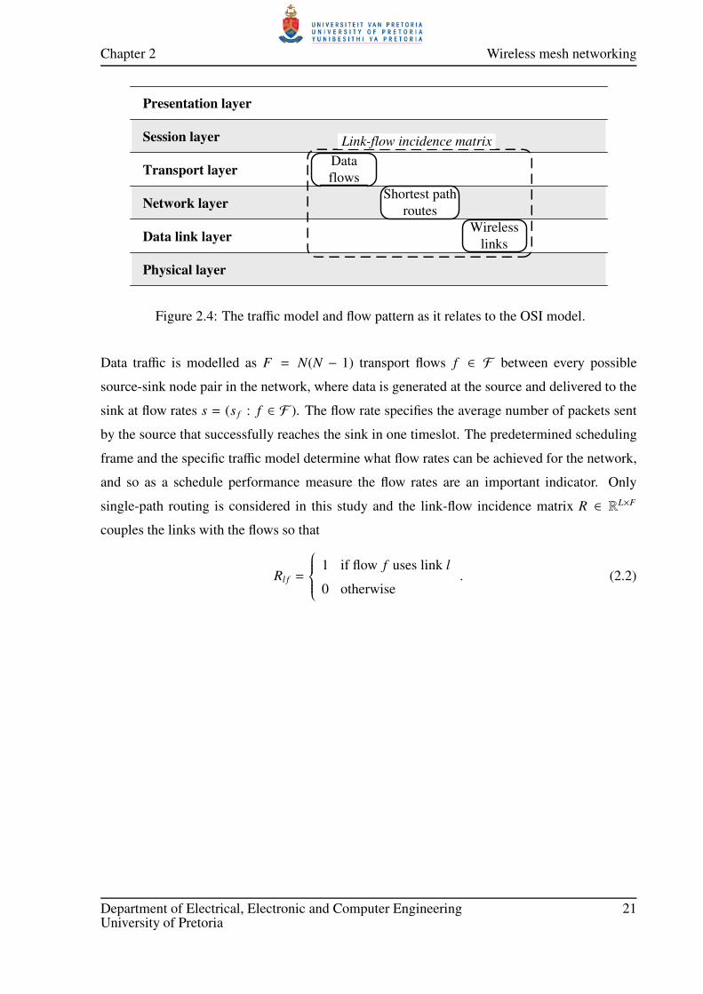
Chapter 2 Wireless mesh networking
Physical layer
Data link layer
Network layer
Transport layer
Session layer
Presentation layer
Data
flows
Wireless
links
Shortest path
routes
Link-flow incidence matrix
Figure 2.4: The traffic model and flow pattern as it relates to the OSI model.
Data traffic is modelled as F = N(N − 1) transport flows f ∈ F between every possible
source-sink node pair in the network, where data is generated at the source and delivered to the
sink at flow rates s = (s f : f ∈ F ). The flow rate specifies the average number of packets sent
by the source that successfully reaches the sink in one timeslot. The predetermined scheduling
frame and the specific traffic model determine what flow rates can be achieved for the network,
and so as a schedule performance measure the flow rates are an important indicator. Only
single-path routing is considered in this study and the link-flow incidence matrix R ∈ RL×F
couples the links with the flows so that
Rl f =
1 if flow f uses link l
0 otherwise. (2.2)
Department of Electrical, Electronic and Computer Engineering 21University of Pretoria

Chapter 2 Wireless mesh networking
Algorithm 1 Dijkstra’s algorithm with the minimum-hop metric.
1: procedure Dijkstra(N)
2: N = Network ⊲ Set of nodes in the network
3: trees=∅ ⊲ To store shortest path trees
4: for i ∈ N do ⊲ For all nodes
5: prev= 0 ⊲ Shortest path tree stores previous hop for each node
6: cost= ∞ ⊲ Tentative cost to node in tree
7: cost(i) = 0 ⊲ Start at root
8: current= i ⊲ Set root as current
9: unvisited= N ⊲ Tree yet to be created
10: while unvisited, ∅ do ⊲ Tree not complete
11: for j ∈ neighbours(current) do ⊲ For all neighbours of current
12: if j ∈ unvisited then
13: cost( j) =cost(current)+1 ⊲ Add one hop
14: prev( j) =current ⊲ Link node to tree
15: end if
16: end for
17: unvisited.remove(current) ⊲ Current becomes visited
18: current=minimumcost neighbour(i) ⊲ Advance current to nearest neighbour
19: end while
20: trees=[trees,prev] ⊲ Add tree map to trees
21: end for
22: end procedure
Department of Electrical, Electronic and Computer Engineering 22University of Pretoria

CHAPTER 3
NETWORK CODING
By regarding information flow on a network as ‘fluid’, nodes are limited to only routing and
forwarding operations. However, when permitting nodes to intelligently code packets together
before a multicast, significant gains in capacity can be achieved [7]. Network coding was
initially studied as it applied to wired networks, and the key concepts were adapted later for
use in wireless networks [8]. A wired network can activate all of its links simultaneously
in a full-duplex manner, which provides complex network coding opportunities. In general,
network coding in wireless networks is simpler to analyse, owing to shared medium access. It
is, however, also the shared medium that provides the network coding opportunities in wireless
networks, which rely on the broadcasting of an NC packet, and opportunistic coding and
listening.
The use of network coding in wired networks is explained in this chapter, and it is shown how
network usage efficiency can be increased with network coding. The throughput bounds that
limit the flow in networks are discussed, as well as the role of network coding in reaching those
bounds. Network coding for wireless networks is looked at, specifically opportunistic coding
or COPE. The implementation aspects of wireless network coding is considered, and a coding
scheme is chosen for use in the wireless mesh networks further considered in this dissertation.
The expected gains with network coding in wireless networks are analysed, and the results are
employed in deciding on the coding scheme. Finally, the operations of network coding are
classified according to their involvement in the OSI network model. An outline of the chapter
content is given in Figure 3.1, indicating the subjects that are covered.
Department of Electrical, Electronic and Computer Engineering 23University of Pretoria

Chapter 3 Network coding
Network
coding
Wired Wireless
Butterfly
network
Max-flow min-cut
theorem
Linear network
coding
Opportunistic
coding
Coding
gain
Coding+MAC
gain
OSI model
analysis
Figure 3.1: Chapter outline for the topics addressed regarding network coding.
3.1 WIRED NETWORK CODING
Networks have always been implemented such that the information flowing through the network
is separated from the coding and transmission mechanisms. This is a restriction which
is removed through the use of network coding. Network coding increases the throughput
of a network by coding on the network level at intermediate nodes. Traditional network
operation involves routing where intermediate nodes only forward received packets and do no
combinations or coding, in contrast to network coded operation.
3.1.1 The butterfly example
A node in a wired network could have one or more separate directed (half-duplex) wired links
to other nodes, and is able to transmit simultaneously and independently on each link. A
directed wireless link can only transmit data in the particular direction of the link, unless the
link is indicated as bidirectional. For the purposes of demonstrating network coding, a packet
transmission is assumed to take one timeslot to be sent and stored in the receiving node buffer.
Copy-based forwarding is employed to route a packet between two nodes that are not directly
connected, unless network coding is specifically done. Network nodes can only transmit or
forward a packet once the packet is fully available in its buffer.
The wired and directed network in Figure 3.2 consists of six nodes (A to F) and seven
directed links, and in the portrayed scenario the objective is to transmit two packets AF (from
Department of Electrical, Electronic and Computer Engineering 24University of Pretoria

Chapter 3 Network coding
A to F) and BE (from B to E). The network topology resembles the image of a butterfly, and is
normally used to explain the concept of wired network coding [9]. Three timeslots are depicted
in the subfigures a) b) and c) of Figure 3.2, where only one forwarding objective is met, namely
the forwarding of packet AF from node A to F. The packet buffer of each node is shown in
a box near the node, and the packets available to the buffer is indicated. If a link is actively
engaged in a timeslot, then the link is emphasised in black and the packet transmitted is noted
on the link. Similarly, if the buffer of a node is accessed in a timeslot, then it is also emphasised
in black.
a)
AF
AF BE
AF BE
A
C
B
D
E F
BE
AF|BE
AF BE
b)
AF
AF
A
C
B
D
E F
BE
AF|BE
AF
AF BE
c)
AF
AFAF
A
C
B
D
E F
BE
AF|BE
AF
AF BE|AF
Figure 3.2: A butterfly network with traditional routing used to relay packet AF in the three
timeslots a) b) and c).
The directed nature of the network in Figure 3.2 makes A-C-D-F the only available path for
the packet AF to be delivered from node A to node F. In the same manner the path B-C-D-E is
the only available path for the forwarding of packet BE. The two nodes C and D along paths
A-C-D-F and B-C-D-E are shared, which causes a congestion, since only one path can use
the contested nodes C and D at any one time. In the first timeslot in Figure 3.2 a) the node C
can receive packets AF and BE at the same time on its two directed links. During the second
timeslot in Figure 3.2 b) the node D receives the packet AF from node C, and in the third
timeslot in Figure 3.2 c) the node F receives its intended packet AF from node D. Thus, with
traditional routing, only one packet can be delivered in three timeslots.
There is congestion at nodes C and D, due to both the paths A-C-D-F and B-C-D-E
required for meeting the delivery objective. A routing mechanism is required to allow the
simultaneous usage of nodes C and D by both routes, in order for both packets AF and BE to
Department of Electrical, Electronic and Computer Engineering 25University of Pretoria

Chapter 3 Network coding
be delivered in three timeslots. Network coding is such a routing mechanism, and it can be
employed when certain conditions are met. Consider the same network and objectives in Figure
3.3, but this time with network coding being used to deliver packet BE as well as packet AF.
a)
AF
AF BE
AF BE
A
C
B
D
E F
BE
AF|BE
AF BE
b)
AF
AF+BE
A
C
B
D
E F
BE
AF|BE
AF+BE
AF BE
c)
AF
AF+BEAF+BE
A
C
B
D
E F
BE
AF|BE
AF+BE
AF|BE BE|AF
Figure 3.3: A butterfly network with network coded routing used to relay packets AF and BE
in the three timeslots a) b) and c).
The important observation is that nodes E and F each has one of the packets received by node C,
and if these sink nodes E and F receive the sum AF+BE then they can recover the packet they
don’t have. For example, if node E has packet AF and receives AF+BE then it can perform
the operation AF+(AF+BE)=BE to recover BE. This operation is true when the packet is
processed as a symbol string in GF(2), where a sum and minus produces the same answer so that
AF+AF=AF-AF=0 and thus (AF+BE)-AF=(AF+BE)+AF=BE. The opportunity is available
at node F, where the node can recover its intended packet AF by performing the operation
BE+(AF+BE)=AF at the end of timeslot three in Figure 3.3 c). In this manner network coding
is used to deliver both packets AF and BE in three timeslots, as opposed to the normal four
timeslots required by traditional routing means.
3.1.2 Max-flow min-cut theorem
Wired networks in particular can be analysed to determine the maximum flow that can be
maintained between a source and sink node. The max-flow min-cut theorem, first proposed
in [10], states that the maximum network throughput between a source and destination node is
bounded by the least throughput en route to the destination. In the butterfly network example
of Figures 3.2 and 3.3 the minimum cut between nodes A and F is one. All the different cut
Department of Electrical, Electronic and Computer Engineering 26University of Pretoria

Chapter 3 Network coding
groupings for the butterfly network are shown in Figure 3.4.
2
A
C
B
D
E F
1
A
C
B
D
E F
2
A
C
B
D
E F
1
A
C
B
D
E F
2
A
C
B
D
E F
a) b) c) d)
e) 2
A C B
D
E
F
f) 3
A
C
B
D
E
F
g) 2
A
C
B
D
E
F
h)
Figure 3.4: All the possible group splittings for a butterfly network.
By splitting the network into two groups, such that the source and sink nodes always belong
to different groups, the cut can be determined as the number of links directed from the source
group to the sink group. The maximum cut in the butterfly network in Figure 3.5 is three, but
this does not mean that a throughput of three packets from node A to node F can be sustained.
The sustainable throughput is limited by the minimum cut, which is one, represented by the
link between node D and node F.
This analysis gives the maximum possible flow between two nodes, but it is the task of
network coding to attempt to achieve that flow. Since traditional routing can only ensure a
throughput of a half, as in the case of Figure 3.2, network coding must be employed to achieve
the full maximum flow. This done by sharing the minimum cut link between the packets AF
and BE. This analysis pertains only to wired networks, where a node can use all of its links
simultaneously.
3.1.3 Linear network coding
In the butterfly network scenario a linear combination of packets forms the network coded
packet, which is effective in relaying the necessary information. It has been constructively
proven in [11] and [12] that linear coding can achieve the max-flow bound between any source
and sink in a directed wired network. Thus the most popular network coding techniques
produce packets which are linear combinations of received packets, since the linearity eases
Department of Electrical, Electronic and Computer Engineering 27University of Pretoria

Chapter 3 Network coding
a)
A
C
B
D
E F
2
1 2
1
2
b)
A
C
B
D
E F
2
32
Figure 3.5: The flow cuts for a butterfly network.
practical implementations [13].
If a node has received n packets M1, . . . , Mn, which might be linear combinations done
at a previous node, then linear network coding combines the packets such that the transmitted
packet or information vector is given by∑n
i=1 giMi. The coefficients g1, . . . , gn, called the
encoding coefficients, are randomly chosen over the same field Fk2
as the packets Mi, where
each packet contains k bits. This allows for distributed operation of network coding. An
efficient distributed randomised approach was proposed in [13] that asymptotically achieves
the multicast capacity given by the max-flow min-cut bound. Random linear network coding
can be used in general multi-source multicast networks with possible correlated sources [14].
3.2 WIRELESS NETWORK CODING
As an introductory example of basic network coding in wireless networks, consider the mesh
subnetwork in Figure 3.6. In this particular instance, a centralised relay node has to forward
two packets in support of the two opposing flows-indicated between nodes A and C. Since A
and C are out of range, the multihop facilities of mesh networks must be employed for their
interconnect. Typically a node in range of both A and C, namely B in this case (alternatively
node E), will serve as a relay that forwards packets between A and C. Therefore A will transmit
a packet (AC), as part of a flow intended for C, which relay B will receive. The packet AC is
received by the neighbours of A, as indicated in the node buffers. In the same way B receives
packet (CA) from sender C, so that the relay is now tasked with the forwarding of both packets
Department of Electrical, Electronic and Computer Engineering 28University of Pretoria

Chapter 3 Network coding
AC and CA. Normal routing dictates that two separate transmissions, and thus two separate
timeslots are needed to fulfil the relaying duty. However, with network coding, the two packets
can be combined and transmitted in one timeslot, with the intended receivers A and C still able
to resolve their respective intended packets CA and AC.
B
F
A D
E C
AC|CA
AC|CA
AC
AC CA
CA
Figure 3.6: Opportunistic two-way wireless network coding, where relay B transmits AC+CA
and both receivers A and C can recover their respective intended packets. Opportunistic
listening and reception reports are not necessary in this instance. Another possibility is for
node E to send the AC+CA packet if node B has other, higher priority packets to transmit.
3.2.1 COPE
COPE (coding opportunistically) is one of the primary examples of network coding in wireless
networks, which relies on opportunistic listening, coding and neighbour state updates to
identify and exploit network coding opportunities [8]. As a wireless forwarding architecture,
COPE operates on a coding layer between the network and data link layers of the OSI
model. It assumes that network nodes forward packets according to an underlying routing
protocol. Opportunistic listening places nodes in promiscuous mode which fills their buffers
with overheard packets, so that the number of network coding opportunities are maximised.
Reception reports and estimation of neighbour buffer content helps a relay in determining
which packets it can potentially code together for a network coded broadcast, as the successful
decoding of the transmission relies on the packets each neighbour has available.
Department of Electrical, Electronic and Computer Engineering 29University of Pretoria

Chapter 3 Network coding
3.2.2 Opportunistic coding
The first condition for a coding opportunity is that a relay should have n > 1 packets that have
to be forwarded to n specific neighbours. Secondly, through reception reports and/or routing
intelligence, the relay must be relatively certain that all n participating neighbours already have
at least n−1 of the n packets. This is a necessary condition; otherwise some receivers might not
be able to decode their packets. To avoid network coding becoming disruptive, a packet must
never be delayed for the sake of network coding it later. This is especially true for prioritised
buffers, where the reshuffling of packets is interpreted by TCP as a congestion signal.
3.2.3 Opportunistic listening
The broadcast nature of wireless networks is advantageous, since it allows for opportunistic
listening. The result is a network with more information at hand, which provides more network
coding opportunities. When the neighbours of a relay possess more overheard packets, then
there are more coding possibilities. While packet snooping creates higher-order network
coding opportunities, it complicates the architecture in an attempt to validate the feasibility
of the opportunities. Integrating reception reporting into a working network, to enable network
coding with opportunistic listening, adds bandwidth and processing overhead as well. For these
reasons, opportunistic listening is not used for the network coding done in this dissertation.
B
F
A D
E C
AD|CA
AD|CA
AD
AD CA
CA
Figure 3.7: Two-way NC requiring opportunistic listening and accurate reception reports to
sink two partial flows in one timeslot. This can be accomplished if the relay node B transmits
AD+CA, since both receivers A and D will be able to extract their intended packets from the
NC sum.
Department of Electrical, Electronic and Computer Engineering 30University of Pretoria
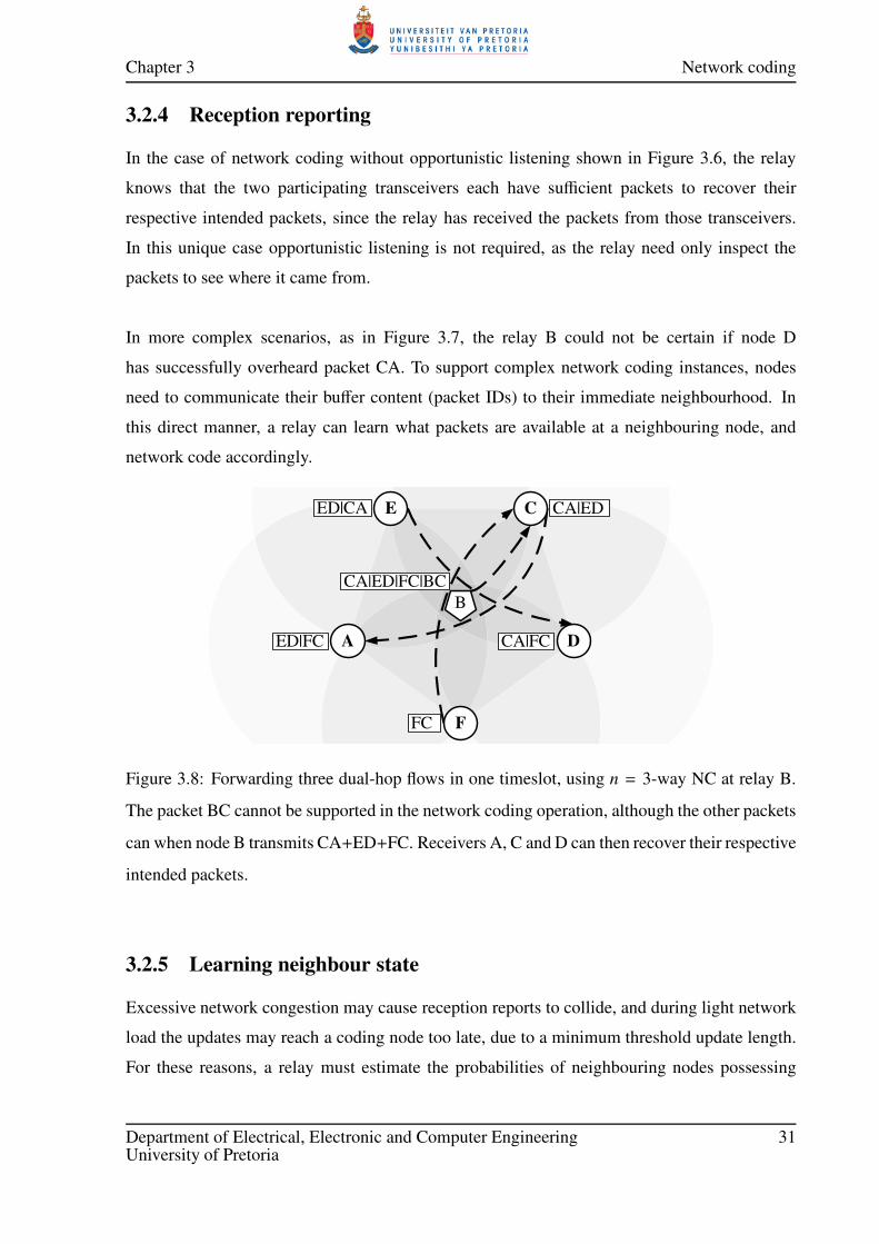
Chapter 3 Network coding
3.2.4 Reception reporting
In the case of network coding without opportunistic listening shown in Figure 3.6, the relay
knows that the two participating transceivers each have sufficient packets to recover their
respective intended packets, since the relay has received the packets from those transceivers.
In this unique case opportunistic listening is not required, as the relay need only inspect the
packets to see where it came from.
In more complex scenarios, as in Figure 3.7, the relay B could not be certain if node D
has successfully overheard packet CA. To support complex network coding instances, nodes
need to communicate their buffer content (packet IDs) to their immediate neighbourhood. In
this direct manner, a relay can learn what packets are available at a neighbouring node, and
network code accordingly.
B
F
A D
E C
CA|ED|FC|BC
ED|CA
FC
ED|FC CA|FC
CA|ED
Figure 3.8: Forwarding three dual-hop flows in one timeslot, using n = 3-way NC at relay B.
The packet BC cannot be supported in the network coding operation, although the other packets
can when node B transmits CA+ED+FC. Receivers A, C and D can then recover their respective
intended packets.
3.2.5 Learning neighbour state
Excessive network congestion may cause reception reports to collide, and during light network
load the updates may reach a coding node too late, due to a minimum threshold update length.
For these reasons, a relay must estimate the probabilities of neighbouring nodes possessing
Department of Electrical, Electronic and Computer Engineering 31University of Pretoria

Chapter 3 Network coding
certain packets, in addition to the perusal of reception reports. Network routing information
allows a relay to estimate the probability that a neighbouring node overheard a packet that
was transmitted to the relay. By performing this investigative analysis, the relay can learn
the buffer content of its neighbours. In the case of an incorrect assumption of neighbour packet
availability, the relay can just retransmit a newly coded packet to the neighbour with insufficient
information. The decision-making process at the relay is illustrated in Figure 3.8.
3.2.6 Coding gain
Network coding gain is defined as the ratio of the number of transmissions required without
network coding, to the number of transmissions needed with network coding to deliver the
same set of involved packets. In the examples of Figures 3.6 and 3.7, the last network coded
transmission consumes one timeslot, instead of the uncoded two. Then, for a total of four
transmissions in the uncoded case, a coding gain of four out of three is achieved. When
opportunistic listening is omitted in Figure 3.7, then no coding gain will be possible.
B
F
A D
E CED|AC|CA
AC|DE
AC|ED DE|CA
CA|ED|DE
AC|CA|DE|ED
Figure 3.9: Cross topology with inadequate information at nodes A (needs packet DE) and D
(needs packet AC). A two-way NC packet AC+DE must first be broadcast by node F, then relay
B can broadcast AC+CA+DE+ED and all receivers will then be able to recover their respective
packets.
One of the key topologies for analysing the coding gain of COPE, is the cross topology [8].
A modified cross topology is shown in Figure 3.9. Normally, if nodes A and D were in direct
contact, a coding gain of eight out of five could be achieved. Uncoded, two transmissions
would be required for each of the four opposing flows, and with network coding the last four
Department of Electrical, Electronic and Computer Engineering 32University of Pretoria

Chapter 3 Network coding
packets forwarded by relay B can be done in one timeslot, to give eight out of five. However,
since A and D are out of range, an extra network coded packet must be broadcast by node F to
give A and D sufficient information to decode the network coded packet to be sent by relay B.
In this case, a smaller coding gain of eight out of six can be achieved.
The assumption is made that all the involved flows have infinite load, and the gain is
determined without regard for the potential coding overhead, loss of coding opportunities, or
packet loss due to medium difficulties. Wireless network coding increases the information
rate above the bit rate, and is able to sustain the capacity increase even during full medium
utilisation. This contrasts with opportunistic routing [15], which only improves utilisation
efficiency when there is little congestion, but does not increase the network capacity.
FE
a)
FE
B
F
A
E
FE
EF EF
B
F
A
E
FE
FE
FEEF
B
F
A
E
FE|EF
FE
FE|EF
FE
B
F
A
E
FE|EF
FE
b) c) d)
EF EF EF
FE|EF
Figure 3.10: Conventional routing without network coding, using an unequal schedule that
gives twice the transmission opportunities to the relay B. Timeslots 1-4 are given in subfigures
a) to d) respectively.
3.2.7 Coding+MAC gain
In the previous analysis of coding gain, the relay node was afforded all the consecutive timeslots
needed to relay its load, as shown in Figure 3.10. In an equal transmission schedule, where
each node receives the same number of timeslots per frame, the relay would quickly become
backlogged as it is unable to forward the same number of packets it receives per frame. This is
where network coding excels in increasing the capacity of the network, since it allows the relay
to sink its acquired load in one timeslot, as shown in Figure 3.11. The network coded packet
Department of Electrical, Electronic and Computer Engineering 33University of Pretoria

Chapter 3 Network coding
multicast in the third timeslot in Figure 3.11 c) contains both of the two packets that required
two separate timeslots to be transmitted without network coding (Figure 3.10). When these two
packets are sent in one timeslot, the limitations of the equal opportunity schedule does not affect
the relay any more. Network coding is then effectively able to double the number of packets
a relay can forward in a scheduling frame, which in turn doubles the capacity, in the case of
Figures 3.6 and 3.7. This gain is termed the coding+MAC (medium access control) gain, which
reflects the actual improvement that is experienced by the network.
FE
a)
FE
B
F
A
E
FE
EF EF
B
F
A
E
FE
FE
FEEF+FE
B
F
A
E
FE|EF
FE
FE|EF
B
F
A
E
FE|EF
FE|EF
b) c) d)
EF EF EF|FE
FE|EF
EF+FE
Figure 3.11: Only three timeslots are required to relay two packets over two dual-hop paths
with network coding. Timeslots 1-4 are given in subfigures a) to d) respectively.
The Coding+MAC gain is the ratio of the number of transmissions needed without network
coding, to the number of transmissions required with network coding, to sink the same set
of involved packets, in a network that gives equal scheduled transmission time to every
participating node. As a continuation of the example shown in Figures 3.10 and 3.11, the
transmissions for the equal schedule without network coding is listed in Table 3.1. Since relay
B can only transmit for one timeslot in the scheduling frame, it is unable to unload the two
packets it acquires each frame. Six timeslots are needed then, as opposed to the case with
network coding, where the relay can unload the two packets it gained in one timeslot.
For proportionally fair schedules, that tend to give greater apparent bandwidth to the more
centralised nodes, the coding+MAC gain is reduced. Relays have more transmission
opportunities, and are able to sink more of the acquired load, reducing the number of
transmissions required. Without opportunistic listening, the maximum possible coding+MAC
gain is two, as evidenced in an analysis of the chain topology discussed in [8]. This gain is also
Department of Electrical, Electronic and Computer Engineering 34University of Pretoria

Chapter 3 Network coding
Table 3.1: The coding+MAC gain for a two-component relay chain, with and without network
coding for equal and unequal scheduling. The equal schedule, in the subgraph at least, allows
the same resources for nodes B, E and F, which for uncoded routing consumes six timeslots to
relay two packets.
Timeslot NC Uncoded Uncoded-equal
1 F-(FE)→B F-(FE)→B F-(FE)→B
2 E-(EF)→B E-(EF)→B E-(EF)→B
3 B-(EF+FE)→F B-(EF)→F B-(EF)→F
4 B-(FE)→E F→B
5 E→B
6 B-(FE)→E
Coding+ 6/3 = 2 6/4 = 1.5 6/6 = 1
MAC gain
achievable, as shown in Table 3.1.
3.2.8 Opportunistic bidirectional wireless network coding
Network coding that can be integrated into wireless mesh network functionality can increase
capacity in the absence of opportunistic listening or reporting overhead, without the need for
control messaging additions. This eases the upgrade of existing networks, and simplifies the
operation of new networks, which is beneficial. For these reasons, network coding without
opportunistic listening, reception reports or learning of the neighbour states will be employed
in this dissertation.
Wireless mesh networks with opposing data flows provide frequent network coding
opportunities, where opportunistic listening is not needed for network coding to visibly
improve network throughput. In this respect, the term bidirectional is used in terms of data
flows and not as a statement of the directionality of a single wireless link. Two flows that
traverse the same three nodes, but in opposite directions, present a network coding opportunity
where opportunistic listening is not necessary. These network coding opportunities occur
especially in the more central parts of the mesh network, where there is a higher density of
opposing flows as indicated in Figure 3.12.
Department of Electrical, Electronic and Computer Engineering 35University of Pretoria

Chapter 3 Network coding
Figure 3.12: Flow load distribution in a 100-node wireless mesh network with equal flow
meshing, clearly indicating the central tendency of higher loaded pathways, ideal for network
coding without opportunistic listening.
Since the specific scenario depicted in Figure 3.11 achieves the maximum possible
coding+MAC gain of two (no opportunistic listening), network coding will be limited to
opportunities of only this instance. In the case of wireless meshing, the multihop network
moves most of its traffic on centralised ‘arteries’, much like highways in a metropolitan street
system. For equal flow load, this traffic pattern creates ample cross-flow coding opportunities,
which will significantly increase throughput if the network coding of Figure 3.11 is harnessed.
The specific algorithm for opportunistic bidirectional wireless network coding is given in
Algorithm 2.
3.3 THE RELATIONSHIP OF NC TO THE OSI NETWORK MODEL
Cross-layer optimisation is a central theme in this dissertation, and therefore the focus
on network coding, which is a very specific coding policy involving multiple OSI layers.
Essentially, network coding has only been introduced in the last decade, and it requires an
unorthodox integration of decisions on different network layers. There are different types of
network coding that involve different OSI layers, as depicted in Figure 3.13. The relationship of
network coding to the OSI network model is discussed in this section, where reference is made
Department of Electrical, Electronic and Computer Engineering 36University of Pretoria

Chapter 3 Network coding
Algorithm 2 Opportunistic bidirectional wireless network coding algorithm.
1: procedure NetworkCoding(T , L)
2: T = Transmitter ⊲ A node part of active spatial reuse set
3: L = Available links ⊲ Temporal reuse set for T , links on which T may transmit
4: B = TransmitBuffer(T ) ⊲ Buffer of packets to be transmitted by T
5: Fa = ∅ ⊲ To store the first packet that can be forwarded
6: repeat(l ∈ L) ⊲ For every usable link in temporal reuse set
7: R = Receiver(l) ⊲ Receiver node of link l
8: a = FirstPacket(B) ⊲ First packet in transmit buffer
9: while NextHop(a), R do ⊲ Compare the next hop of packet a with receiver
10: Advance(a) ⊲ Use next packet, until entire buffer is checked
11: end while
12: if NextHop(a)= R then ⊲ Suitable packet has been found
13: Fa = a ⊲ Store for future use
14: end if
15: until Fa , ∅16: if PrevHop(Fa)∈ L then ⊲ Temporal reuse set allows for NC
17: Fb = FirstPacket(B) ⊲ First packet in transmit buffer
18: while NextHop(Fb),PrevHop(Fa) or NextHop(Fa),PrevHop(Fb) do
19: Advance(Fb) ⊲ Use next packet, until entire buffer is checked
20: end while
21: if NextHop(Fb)=PrevHop(Fa) and NextHop(Fa)=PrevHop(Fb) then
22: FNC = Fa + Fb ⊲ Network coded packet
23: end if
24: end if
25: end procedure
Department of Electrical, Electronic and Computer Engineering 37University of Pretoria

Chapter 3 Network coding
to specific kinds of coding approaches and how the network layers are involved.
Physical layer
Data link layer
Network layer
Transport layer
Session layer
Presentation layer
Application layer
Network
coding Physical layer
Network coding
Application layer Network coding
Figure 3.13: Various network coding opportunities in relation to the supporting OSI layers.
3.3.1 Application layer network coding
Random linear network coding is used in Avalanche [16], a peer-to-peer content distribution
application by Microsoft. Operating only on the application layer, this type of network coding
transmits random linear combinations of packets, together with the encoding vector values,
from the server and between the peers. A distribution server divides a file into blocks and
network codes blocks together in this manner, so that when a peer has enough randomly
coded blocks, the peer can reconstruct the original file. Diversity is afforded through the linear
combinations, which make the solution robust against servers leaving early or peers connecting
only for the download duration.
As another example of network coding for peer-to-peer content distribution, R-squared
was implemented in [17]. Suitable for live peer-to-peer streaming, this protocol takes full
advantage of random network coding. A randomised push algorithm is used to relieve peers
from having to explicitly request segments. Random network coding is used for each segment,
so that multiple peers can serve a client without incurring a messaging overhead. The decoding
complexity is reduced with dense linear codes, and priority to segments close to the playback
point is given, so that new peers enjoy short buffering delays. These examples serve only to
illustrate network coding as it relates to the application layer, and will not be considered further
in this dissertation.
Department of Electrical, Electronic and Computer Engineering 38University of Pretoria

Chapter 3 Network coding
3.3.2 Network layer
At the network layer, a relay node has to evaluate its packet buffer in the context of its routing
table to recognise network coding opportunities. When opportunistic listening is involved, it
even has to take into consideration the buffers of neighbouring nodes. Also, in the absence of
opportunistic listening, a relay node can inspect a set of packets to infer the buffer content of
the original senders of that packet. When taking into account the intended receivers of those
packets, a relay can decide whether neighbours have sufficient information to process a network
coded packet.
3.3.3 Data link layer
The data link layer is concerned with transmission over a direct link, and since a relay activates
two direct virtual links (multicast), the network coding operation have aspects in this layer as
well. Indeed, we show in this work, that channel forward error-correction coding and network
coding can become one coding operation. Still, routing decision and intelligence at the network
layer is involved for successful network coding, as shown in Figure 3.13.
3.3.4 Physical layer network coding
Even more efficient than conventional wireless network coding is physical layer NC [18],
although from a signal processing perspective it is more complex. Understanding that the relay
typically does not need the individual packets itself, from which the NC packet is formed, one
can go one step further and subsume the communication of the two packets into one timeslot
instead of two. So in the example of Figure 3.6, physical network coding allows nodes A and
C to transmit their packets AC and CA to relay B at exactly the same time. Here receiver B
records the superposition of packets AC and CA, which is in fact a physical layer NC packet.
Relay B does not need to separate the two packets; instead it only needs to transmit their sum.
Since receivers A and C know the waveform they originally transmitted to B, they can just
subtract it from the sum broadcast by relay B to recover their intended packets.
The complication of physical layer network coding is due to wide scope of optimisation
spread over three OSI layers. Intricate scheduling decisions now have to be made by not
just the relay, but all nodes involved in the network coding operation. This requires network
layer and data link layer knowledge about routing and medium access control. Fitting
Department of Electrical, Electronic and Computer Engineering 39University of Pretoria

Chapter 3 Network coding
forward error-correction coding has to be chosen that complements the unique superpositions
experienced on the physical layer. For the best performance, the implementation of physical
network coding requires a cross-layer optimised design, across the base OSI layers. This type
of network coding will, however, not be used in this work.
Department of Electrical, Electronic and Computer Engineering 40University of Pretoria

CHAPTER 4
SCHEDULE ASSIGNMENT
The methodology of sharing the capacity of one medium between a network of nodes is
considered in this chapter. Regulating access to the wireless communication medium is one of
the key aspects of wireless scheduling, and the different means of access control are discussed.
The problems of dynamic medium access and scheduling are explained, and the use of
predetermined scheduling is further motivated. Definitions and examples are used to illustrate
time and space-time division multiple access, which are used in particular for this study. The
relation of scheduling to the OSI model is explained and used to indicate the importance of
scheduling in the operation of wireless mesh networks. An algorithm for initial wireless mesh
network scheduling is proposed, which is crucial for schedule optimisation and the relaying of
new improved schedules in ad hoc networks.
The different manners in which a scheduling frame is populated are explored in this
chapter, in particular link and node-assignment. The best situations for and the benefits of each
schedule assignment method are discussed, and the results are used to explain the superiority of
link-assignment with extended transmission rights. The different schedule assignment methods
are analysed in terms of the two concepts of packet depletion and temporal reuse, which are
newly defined in this work. It is shown that link-assignment with extended transmission rights
can achieve higher schedule usage efficiency and allow for network coding, owing to the added
measure of temporal reuse. Figure 4.1 shows the main topics that are covered in this chapter.
Department of Electrical, Electronic and Computer Engineering 41University of Pretoria

Chapter 4 Schedule assignment
Schedule
assignment
Medium
access control
Dynamic
MACTDMA STDMA OSI model
analysis
Assignment
methods
Link-
assignment
TDMA STDMA
Node-
assignment
TDMA STDMA
Initial
scheduling
Temporal
reuse
Utilisation
efficiency TDMA STDMA
Figure 4.1: The chapter outline of schedule assignment topics discussed.
4.1 MEDIUM ACCESS CONTROL
The network topology defines the usable wireless links in a mesh network, but transmission
over those channels has to be coordinated for successful network operation. Local mesh clients
have access to the same medium, which has to be shared to provide a transmission opportunity
for all links. The communication resource of limited bandwidth has to be rationed in a manner
that maintains the threshold SINR of activated links.
Two of the primary methods of bandwidth sharing is frequency division multiple access
(FDMA) and time division multiple access (TDMA), where either the frequency band or a time
period is divided into segments which are assigned to certain links. Frequency or time segments
can be made equal, or unequal, but equality is preferable since it is more amenable to the use of
synchronisation. For improved bandwidth management even both multiplexing methods can be
employed together, where, for example, an FDMA bandwidth segment is utilised by multiple
links through TDMA division of the sub-band. This study will focus on scheduling under the
TDMA regime with equal-length timeslots, since time division multiplexing is instrumental in
the cross-layer optimisation undertaken in this dissertation.
A distinction is made between predetermined and dynamic scheduling, for either fixed
or variable-length timeslots under TDMA. Network nodes that transmit according to the same
deterministic network scheduling algorithm, or preset pattern, are not plagued by dynamic
MAC issues such as the hidden terminal problem. Predetermined schedules have an affinity for
Department of Electrical, Electronic and Computer Engineering 42University of Pretoria

Chapter 4 Schedule assignment
centralised optimisation, whereas dynamic scheduling involves primarily ad hoc decentralised
node operation which is difficult to incorporate in a global optimum. Dynamic scheduling
requires more complicated control signalling to manage medium contention, which is not
required with predetermined scheduling under synchronisation. The difficulties of dynamic
scheduling are explained in greater detail in the following subsection.
4.1.1 Dynamic medium access control difficulties
Medium access control in wireless mesh networks is a difficult problem due to the hidden
terminal effect, and for dynamic schedules only non-perfect solutions can be achieved. Two
potential transmitters want to communicate with a specific receiver, but if the transmitters are
out of sensing range of each other then the second transmitter will interrupt a transmission from
the first. Multiple access collision avoidance (MACA [19]) RTS/CTS (request to send/clear to
send) handshaking improves the chances for successful data transmission, where the receiver
transmits a CTS message to only one of possibly several senders who transmitted contending
RTS messages to the receiver. When a sender requires a transmission opportunity it transmits an
Node A
Node B
Node C
Node R
Data
transmission
Collision
Figure 4.2: The hidden terminal effect. Sender A is busy transmitting to receiver R, but because
sender C is too far from A it falsely believes it has a transmission opportunity.
RTS message declaring its need for access to the receiver, as shown in Figure 4.2. The receiver
then processes all the RTS messages and with fair access in mind, broadcasts a CTS message
stating which sender has the right for data transmission. The RTS/CTS messages contain the
sender and receiver addresses, the required length of transmission time et cetera in order for the
mesh neighbourhood is aware of the planned medium usage.
Department of Electrical, Electronic and Computer Engineering 43University of Pretoria

Chapter 4 Schedule assignment
A
R
C
B
RTS
RTS
RTS
CTS
DATAACK
Figure 4.3: Multiple access collision avoidance for wireless (MACAW) where candidate
senders contend for a data transmission opportunity using RTS/CTS handshaking.
By acknowledging the correct receipt of the sender’s data, the receiver can improve reliability.
This is done in multiple access collision avoidance wireless (MACAW [20]), which operates
according to the handshake RTS-CTS-DATA-ACK indicated in Figure 4.3. The difficulty
of MAC persists since collisions can occur during the RTS message contention phase.
Floor acquisition multiple access (FAMA [21]) addresses this issue in part, by requiring
that candidate senders sense the channel before broadcasting the RTS, in other words
CSMA-RTS-CTS-DATA-ACK. The separation of the control messaging and data transmission
is effective in alleviating the hidden terminal problem, although it cannot completely ensure
RTS-phase non-collision. Another approach is to have receiver initialised MAC, where
transmission authorisation is given to a potential sender by the receiver via a ready-to-receive
RTR message. In this manner the receiver polls all of its neighbours to give them a
transmission opportunity, as shown in Figure 4.4, and to inform non-intended senders that
the sanctioned sender will communicate with the receiver. The RTR-DATA-ACK handshake
is employed in multiple access collision avoidance by invitation (MACA-BI [22]) for its
ability to avoid collisions during the DATA phase. Control collisions, particularly RTR
clashes, can still occur due to the hidden terminal effect. When an RTR collision occurs, a
no-transmission-request (NTR) is broadcast to forbid the data transmission. Receiver initialised
multiple access - dual polling (RIMA-DP [23]) improves on MACA-BI by allowing a reverse
data transmission from the receiver to the sender, in an attempt to minimise control messaging.
An RTR-DATA-DATA-ACK handshake is used by RIMA-DP for this purpose.
Department of Electrical, Electronic and Computer Engineering 44University of Pretoria
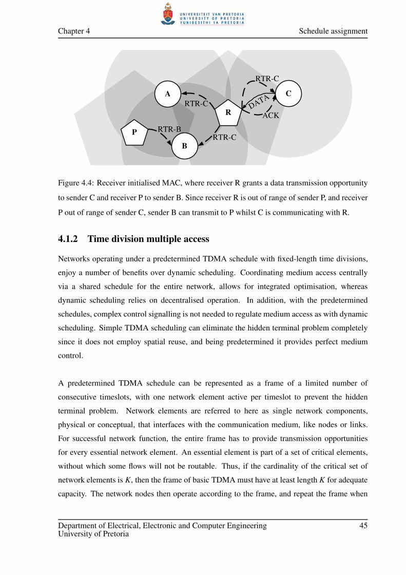
Chapter 4 Schedule assignment
R
C
RTR-C
P
DATA
ACK
A
B
RTR-C
RTR-CRTR-B
Figure 4.4: Receiver initialised MAC, where receiver R grants a data transmission opportunity
to sender C and receiver P to sender B. Since receiver R is out of range of sender P, and receiver
P out of range of sender C, sender B can transmit to P whilst C is communicating with R.
4.1.2 Time division multiple access
Networks operating under a predetermined TDMA schedule with fixed-length time divisions,
enjoy a number of benefits over dynamic scheduling. Coordinating medium access centrally
via a shared schedule for the entire network, allows for integrated optimisation, whereas
dynamic scheduling relies on decentralised operation. In addition, with the predetermined
schedules, complex control signalling is not needed to regulate medium access as with dynamic
scheduling. Simple TDMA scheduling can eliminate the hidden terminal problem completely
since it does not employ spatial reuse, and being predetermined it provides perfect medium
control.
A predetermined TDMA schedule can be represented as a frame of a limited number of
consecutive timeslots, with one network element active per timeslot to prevent the hidden
terminal problem. Network elements are referred to here as single network components,
physical or conceptual, that interfaces with the communication medium, like nodes or links.
For successful network function, the entire frame has to provide transmission opportunities
for every essential network element. An essential element is part of a set of critical elements,
without which some flows will not be routable. Thus, if the cardinality of the critical set of
network elements is K, then the frame of basic TDMA must have at least length K for adequate
capacity. The network nodes then operate according to the frame, and repeat the frame when
Department of Electrical, Electronic and Computer Engineering 45University of Pretoria

Chapter 4 Schedule assignment
its end is reached to give continued transmission capacity for the wireless mesh network.
4.1.3 Space-time division multiple access
Nodes in wireless multihop mesh networks generally have a significant transmit radius smaller
than the mesh radius, such that multiple hops are required to deliver the longest flows (in terms
of hops). This creates a scenario where possibly multiple transmissions can be active in the
same timeslot, without the particular receivers experiencing interruption. The opportunity for
multiple active links at the same time is termed spatial reuse, since there is a significant spatial
distance between the activated links. The necessary condition for a valid spatial reuse set, is
for each receiver in the link-set to have sufficient SINR, given the set of activated transmitters.
Space-time division multiple access (STDMA) and TDMA are equivalent when all spatial
reuse groups in STDMA have only one transmitter. Otherwise, STDMA provides a more
efficient schedule, packing more network elements into each timeslot than TDMA.
When the mesh network has a larger average flow hop-count, then the links are more
removed in space, and the spatial reuse potential is higher. As the spatial reuse set grows
larger, the interference increases from the larger number of transmitters. For denser networks,
the threshold SINR may be reduced in order to increase spatial reuse, so that the network
can service greater numbers of mesh clients. This is the trade-off that makes the high-noise
channel coding region relevant to STDMA networks, since lower SINR means stronger coding
is required to combat the high interference. Later in this dissertation, this coding region will be
addressed to allow for dense mesh deployments of the future.
4.1.4 Scheduling and the OSI model
Transmission scheduling, whether fixed or dynamic, defines most operational and functional
aspects of the wireless mesh network. The timing of a link transmission, the power used,
the listening receivers and the achievable flow rates, are all subject to the active schedule.
The power limits and transmission rates of each scheduled link is part of the physical layer
definition, which sets the power and modulation scheme a link should use when transmitting in
a particular timeslot. Regulating access to the communication medium is one of the schedule’s
most important tasks, to permit transmission rights to all links in spite of the limited bandwidth.
This functionality resides in the MAC sub-layer of the data-link OSI layer, and it ensures that
Department of Electrical, Electronic and Computer Engineering 46University of Pretoria

Chapter 4 Schedule assignment
each intended receiver has a sufficient SINR.
The links defined in the data-link layer are related to the network flows, defined in the
network layer, via the link-flow incidence matrix R given in Chapter 3. The schedule should
use the link-flow incidence matrix as an optimisation tool, since R gives the relative routing
loads of the links, which are important utility measures. In the transport layer the flow rates are
regulated, and here the design of a schedule affects the achievable rates. The higher OSI layers
are thus concerned with flow fairness and rates, and the transmission scheduling can be set up
so that certain flow objectives can be realised. The relation of transmission scheduling to the
OSI model is indicated in Figure 4.5.
Physical layer
Data link layer
Network layer
Transport layer
Session layer
Presentation layer
Data
flows
Wireless
links
Shortest path
routes
Link-flow incidence matrix
Transmitter Power
and Modulation
Medium access
control
Flow rate
control
Routing
control
Figure 4.5: Transmission scheduling in relation to the OSI layers.
4.2 SCHEDULE ASSIGNMENT METHODS
Given the user multiplexing method of TDMA, with or without spatial reuse, a schedule
assignment strategy has to be formulated to actually assign capacity for the network. If only
a transmitter or receiver is scheduled, then the bandwidth sharing becomes dynamic and the
hidden terminal problem becomes an issue. Thus, the smallest network element that can be
scheduled is a single directed link. A transmitter node can also be scheduled, or at least the set
of outgoing links pertaining to a certain node, to clearly control medium access.
The two predominant transmission schedule assignment methods are thus node- and
link-assignment, and while node-assigned schedules [24, 25] can perform NC and have better
Department of Electrical, Electronic and Computer Engineering 47University of Pretoria

Chapter 4 Schedule assignment
usage efficiency, they lack the higher spatial reuse and finer granularity for optimisation
achieved by link-assigned schedules [26–28]. Preference is given to link-assignment since it is
more amenable to cross-layer optimisation and it can achieve greater capacity owing to better
spatial reuse. In this subsection illustrations of the workings of these two assignment methods
are given, both with and without spatial reuse, and their properties are discussed.
Initial schedule assignment is discussed in this section, to address how a newly formed
or changed mesh network communicates topology information for centrally optimising a
schedule. This first schedule assignment is crucial to obtain an optimised schedule, and to
update mesh clients with new schedules. The schedule, as a form of medium access control, is
required for the control signalling and information gathering that can allow for more refined
schedules to be calculated and advertised.
4.2.1 Link assignment
The most basic network element that can be scheduled in a timeslot is a directed wireless link
from one transmitter node to another single receiving node. A complete and valid TDMA
scheduling frame must provide capacity for the critical link set, so that all network flows can
be routed. Whether for simplex TDMA or when the spatial domain is reused, the active spatial
reuse set must allow for adequate receiver SINR as formulated in Equation 2.1.
Since links are not grouped together as in node-assigned scheduling, greater assignment
variation is possible with spatial reuse, which gives better optimisation results. Another benefit
owing to the finer granularity is improved spatial reuse, although the resultant temporal reuse is
non-existent. Network coding is not possible with a link-assigned schedule, unless transmission
rights are extended. Typically, link-assigned schedules have longer frames, but no node-based
scheduling algorithm is required as with node-assigned scheduling. A link-assigned schedule
contains a complete MAC definition, as opposed to node-assigned scheduling where each node
needs to manage the transmissions on its various links.
4.2.1.1 Link-assigned TDMA
An example of link-assigned TDMA network operation is shown in Figure 4.6. The arrays of
short vertical lines represent the links in the network and indicate in bold lining the currently
Department of Electrical, Electronic and Computer Engineering 48University of Pretoria

Chapter 4 Schedule assignment
activated link for the particular timeslot. Only one link is permitted to transmit in any timeslot
for link-assigned TDMA, and this is the case for the specific schedule in Figure 4.6. For L links,
it is then clear that the most basic TDMA schedule will require also L timeslots to satisfy the
critical link demand. Since no spatial reuse is utilised, the original link definitions still hold, so
all links are assumed to have sufficient SINR by design.
Timeslot 1 Timeslot 2 Timeslot 3 Timeslot 4
Timeslot 5 Timeslot 6 Timeslot 7 Timeslot 8
Figure 4.6: The first eight timeslots in a simplex TDMA scheduling frame of length 14, for a
sample multihop mesh network.
4.2.1.2 Link-assigned STDMA
When a set of links are sufficiently removed in space, such that their receivers do not receive
significant interference, then that set can be scheduled in one timeslot. The SINR requirement
formulated in Equation 2.1 will be met by a valid spatial reuse group. In Figure 4.7 an example
of link-assigned STDMA is shown, where in some timeslots multiple links are scheduled
simultaneously. In the first timeslot the two indicated links may transmit at the same time
for the duration of the timeslot, since each receiver has sufficient SINR. The schedule is
set up so that each network link has at least one timeslot available for transmission, but the
specific schedule will not necessarily give the best performance. This is the case since the
single link in timeslot seven allows for other links to transmit simultaneously, but the example
serves only to illustrate the concept of link-assigned STDMA. The result is a schedule that has
half the size of a plain TDMA schedule, due to an average spatial reuse of two links per timeslot.
The link-assigned STDMA schedule employed in the simulations of this dissertation,
Department of Electrical, Electronic and Computer Engineering 49University of Pretoria

Chapter 4 Schedule assignment
uses a packing heuristic [29], which packs as many links as have not yet transmitted into a
timeslot. The scheduling program is shown in Algorithm 3, where spatial reuse groups are
formed with maximum link inclusion, first satisfying links with positive demand. An urgency
value assigned to each link gives preference to links which were included a longer time ago.
When the unsatisfied links have been checked for possible inclusion, the satisfied links are
checked as well to maximise spatial reuse. The procedure SimultaneousLinkValid()
checks if the threshold SINR values are met for all receivers in the expanded spatial reuse
clique, if a link addition is made. Since some links carry more traversing flows, like the more
centrally located ones, a traffic-adaptive version of this algorithm can also be used as in [30].
The traffic-adaptive version will give higher demands for links routing more flows, to create a
fairer schedule.
Timeslot 1 Timeslot 2 Timeslot 3 Timeslot 4
Timeslot 5 Timeslot 6 Timeslot 7
Figure 4.7: Non-optimal link-assigned STDMA seven-slot frame satisfying critical capacity
demand.
4.2.2 Node assignment
Instead of scheduling single links, single nodes can be assigned to timeslots in a TDMA
schedule. The nodes that are assigned serve the role of transmitter, but successful medium
access is guaranteed, unlike with dynamic MAC such as MACAW where collisions can still
occur during the RTS message contention phase. This is achieved by ensuring adequate SINR
for the receivers of each outgoing link of the scheduled node, especially when spatial reuse is
considered. However, since a collection of links pertaining to a certain node has to contend
for the same timeslot, each scheduled node has to execute a scheduling algorithm of its own to
Department of Electrical, Electronic and Computer Engineering 50University of Pretoria

Chapter 4 Schedule assignment
share a timeslot between multiple links. So, while node-assigned schedule frames tend to be
shorter than link-assigned frames, extra control and definition is required at the nodes, which
reduces optimality. Since all the outgoing links of a node is scheduled in one timeslot, such
a schedule enjoys full temporal reuse. Node-assigned schedules do, however, not in general
achieve the spatial reuse of link-assigned schedules. The simultaneous grouping of the links of
a node also gives less optimisation control.
4.2.2.1 Node-assigned TDMA
Assigning one transmitter node to a timeslot is a very basic way to create a TDMA schedule, as
displayed in Figure 4.8. The default link SINR values are maintained, since only one transmitter
is active, and so no SINR adequacy checking is required. Seeing that all outgoing links of a node
is scheduled in the same timeslot, the resulting schedule frame is shorter than with link-assigned
TDMA. It should be noted that the set of scheduled links do not simultaneously transmit in one
timeslot, but the timeslot is rather reused over successive frame repetitions to serve all the
links. Due to this extra node-based scheduling requirement, a node-assigned schedule is not
necessarily more efficient (in terms of throughput) than a link-assigned one.
Timeslot 1 Timeslot 2 Timeslot 3 Timeslot 4
Timeslot 5 Timeslot 6 Timeslot 7
Figure 4.8: A node-assigned TDMA equivalent of the example in Figure 4.6.
4.2.2.2 Node-assigned STDMA
Multiple nodes can also be scheduled simultaneously, although the spatial reuse tends to be less
than with link-assigned scheduling. This is due to the fact that more links at each node should
have sufficient SINR, which increases the areas of influence in the network. The reduced
Department of Electrical, Electronic and Computer Engineering 51University of Pretoria

Chapter 4 Schedule assignment
Algorithm 3 Link-assigned STDMA schedule assignment algorithm.
1: procedure LinkSTDMA(L)
2: D= (D(l) = 1, l ∀L) ⊲ Demand: Link once or the number of flows using the link
3: U= (U(l) = 1, l ∀L) ⊲ Urgency: When last was a link included?
4: A= L; B= ∅; S= ∅ ⊲ Unsatisfied links; Satisfied links; Empty schedule
5: repeat ⊲ Until all links satisfied
6: Atemp=A; Btemp=B; L= ∅ ⊲ Temporary arrays; Empty spatial reuse linkset
7: repeat ⊲ Until all unsatisfied links checked
8: l = argm∈Atempmax (D(m) · U(m)) ⊲ Link with maximum demand×urgency
9: if SimultaneousLinkValid(L, l) then ⊲ Can add link to set
10: L.add(l); D(l)=D(l)-1; U(l)=0 ⊲ Extend linkset; Reduce demand, urgency
11: if D(l)= 0 then ⊲ Satisfied
12: B.add(l); A.remove(l) ⊲ Not unsatisfied
13: end if
14: end if
15: Atemp.remove(l) ⊲ Link already checked
16: until Atemp= ∅ ⊲ Check all unsatisfied links
17: repeat ⊲ Until all satisfied links checked
18: l = argm∈Btempmax (D(m) · U(m)) ⊲ Link with maximum demand×urgency
19: if SimultaneousLinkValid(L, l) then ⊲ Can add link to set
20: L.add(l); U(l)=0 ⊲ Extend linkset, null urgency
21: end if
22: Btemp.remove(l) ⊲ Link already checked
23: until Btemp= ∅ ⊲ Check all satisfied links
24: S=[S, L] ⊲ Add spatial reuse linkset to schedule
25: until (B= L) ⊲ Is there an unsatisfied link?
26: end procedure
Department of Electrical, Electronic and Computer Engineering 52University of Pretoria

Chapter 4 Schedule assignment
spatial reuse can be seen in Figure 4.9, where an average spatial reuse of 7/4 < 2 is achieved,
which is less than with link-assigned STDMA. Temporal reuse is increased with node-assigned
STDMA however, and a temporal reuse of 8/4 = 2 is achieved here. This schedule frame is
even shorter than link-assigned STDMA, owing to the high temporal reuse and spatial reuse,
but its efficiency is not necessarily greater.
Similar to the link-assigned STDMA scheduling Algorithm 3, node packing is done to
maximise spatial reuse in node-assigned STDMA scheduling shown in Algorithm 4.
Unsatisfied nodes are first checked if they can be successfully included into a spatial reuse
node group, then satisfied links are checked, with the goal of spatial reuse maximisation.
The function SimultaneousNodeValid() establishes whether the inclusion of a new node
will cause the involved link SINR values to decrease below the threshold. When a node
can be added such that all the links of all the included nodes have sufficient SINR values,
then the clique is extended. The traffic-adaptive version assigns node demands according
to the collective flow load experienced by the links of a certain node, to deliver a more fair
transmission schedule.
Timeslot 1 Timeslot 2 Timeslot 3 Timeslot 4
Figure 4.9: A more compact node-assigned STDMA schedule with spatial reuse.
4.2.3 Initial scheduling
During mesh network deployment, each node n gets a unique timeslot assignment tn ∈ [1, T ], in
a TDMA frame of length T . Node clocks are also synchronised, so that each node will transmit
during the correct timeslot. A global or local synchronisation pilot signal can be established
Department of Electrical, Electronic and Computer Engineering 53University of Pretoria

Chapter 4 Schedule assignment
Algorithm 4 Node-assigned STDMA schedule assignment algorithm.
1: procedure NodeSTDMA(N)
2: D= (D(n) = 1, n ∀N) ⊲ Demand: Node once or the number of flows using the node
3: U= (U(n) = 1, n ∀N) ⊲ Urgency: When last was a node included?
4: A= N ; B= ∅; S= ∅ ⊲ Unsatisfied nodes; Satisfied nodes; Empty schedule
5: repeat ⊲ Until all nodes satisfied
6: Atemp=A; Btemp=B; N= ∅ ⊲ Temporary arrays; Empty spatial reuse nodeset
7: repeat ⊲ Until all unsatisfied nodes checked
8: n = argm∈Atempmax (D(m) · U(m)) ⊲ Node with maximum demand×urgency
9: if SimultaneousNodeValid(N, n) then ⊲ Can add node to set
10: N.add(n);D(n)=D(n)-1;U(n)=0 ⊲ Extend nodeset; Reduce demand, urgency
11: if D(n)= 0 then ⊲ Satisfied
12: B.add(n); A.remove(n) ⊲ Not unsatisfied
13: end if
14: end if
15: Atemp.remove(n) ⊲ Node already checked
16: until Atemp= ∅ ⊲ Check all unsatisfied nodes
17: repeat ⊲ Until all satisfied nodes checked
18: n = argm∈Btempmax (D(m) · U(m)) ⊲ Node with maximum demand×urgency
19: if SimultaneousNodeValid(N, n) then ⊲ Can add node to set
20: N.add(n); U(n)=0 ⊲ Extend nodeset, null urgency
21: end if
22: Btemp.remove(n) ⊲ Node already checked
23: until Btemp= ∅ ⊲ Check all satisfied nodes
24: S=[S, N] ⊲ Add spatial reuse nodeset to schedule
25: until (B= N) ⊲ Is there an unsatisfied node?
26: end procedure
Department of Electrical, Electronic and Computer Engineering 54University of Pretoria

Chapter 4 Schedule assignment
to guide the timings of all nodes. Now, with the simple predetermined TDMA schedule, each
node transmits at maximum power Pmax during their timeslot. Each node records the power
received for each timeslot in the frame, with the purpose of forming a topology image from the
resulting interference matrix J. Node j will record received interference power Ji j during the
timeslot of node i, and from this the gain Qi j = Ji jP−1max can be calculated.
Once an entire frame has been cast, a second frame commences wherein each node i
broadcasts its interference vector J∗i. Each neighbouring node with sufficient SNR stores the
overheard vector, and forward broadcasts it together with its own interference vector and other
overheard vectors. This topology broadcast continues until all nodes have forwarded all their
own and overheard interference vectors. In this manner, an IGW or other powerful processing
node can obtain the interference matrix J and consequently the gain matrix Q. Having these
measures, the simple link-assigned TDMA schedule can be replaced throughout the network
with a schedule optimised at a central node.
4.3 TEMPORAL REUSE
Spatial reuse is the reuse of a timeslot by simultaneously activated links, with sufficient SINR,
in the spatial domain. Likewise, temporal reuse is defined here as the reuse of a timeslot by a
group of links in the time domain. A temporal reuse group is the set of outgoing links from
a particular node that may transmit in a certain timeslot. Since a transmission schedule is
composed of a T -length frame that is repeated in time, every timeslot in the frame is repeated
at frequency 1/T . This means that the links in a temporal reuse group will share the capacity
of a timeslot over all the repetitions of the timeslot in which the temporal reuse group appears.
The reuse of a timeslot in the time domain thus refers to a timeslot, at a particular location in
the scheduling frame, that is reused by a group of links as the specific timeslot reoccurs with
the repetition of the frame in time.
Node-assigned schedules enjoy full temporal reuse, at the expense of secondary schedule
requirements at transmitting nodes. A measure of temporal reuse can be given to link-assigned
schedules, without the need for additional scheduling policies, by assigning priorities to links
in the temporal reuse sets. This prioritised temporal reuse for link-assigned scheduling was
Department of Electrical, Electronic and Computer Engineering 55University of Pretoria

Chapter 4 Schedule assignment
first proposed in [1] as link-assignment with extended transmission rights (LET), although the
relationship to temporal reuse was not brought to light. This section extends the work in [1] by
characterising the networks that can benefit from temporal reuse, in terms of the concepts of
packet depletion and temporal reuse that are newly defined in this work.
Packet depletion is defined here (and in [31]) as the condition where a scheduled link
does not have packets to transmit, resulting in a wasted timeslot with link-assigned scheduling.
When a transmitting node does not have a packet ready for a scheduled link, then the timeslot
can be used to transmit on another link instead. In this manner, a timeslot is reused by multiple
links over the continuous repetition of the limited-length scheduling frame. Temporal reuse is
important in transmission scheduling, as it is a means to share capacity and improve schedule
usage efficiency. This term is explained further in this section, and the networks that can have
improved efficiency with temporal reuse are also characterised.
4.3.1 Motivation
Node-assigned schedules [24] have to employ a form of temporal reuse to provide capacity for
every outgoing link associated with a scheduled node. Here secondary scheduling is involved,
where every node has to decide how to divide its available capacity between its outgoing links.
Having multiple link options per node results in higher capacity usage efficiency, at the expense
of reduced spatial reuse. Due to packet depletion, node-assigned schedules can achieve higher
usage efficiency than normal link-assigned schedules. The downside is reduced spatial reuse,
since the scheduling of all the links of a node extends the interference.
Alternatively, link-assigned schedules with extended transmission rights can achieve
some measure of the same improved efficiency of node-assigned scheduling with better
spatial reuse, which results in a higher schedule capacity. A spatial reuse group is first
established, as with normal link-assigned STDMA, and then transmission rights are extended
to all alternate links, of scheduled nodes, with sufficient SINR. The links in the extended
temporal reuse set are prioritised primarily so that secondary scheduling is not required, which
would complicate global optimisation. The link prioritisation sets LET apart from temporal
reuse in regular node-assigned scheduling, and prioritisation also serves to allow for a more
concise network capacity estimation under temporal reuse. The initial spatial reuse group
Department of Electrical, Electronic and Computer Engineering 56University of Pretoria

Chapter 4 Schedule assignment
forms the highest priority linkset, and the additional links are further given lower priorities
on a node-centric basis. This means that the reserve links of a node are assigned different
priorities, and that links from other nodes are not involved in that particular priority assignment.
In addition, by extending a link assignment to a prioritised group of links, the schedule
allows for the implementation of opportunistic network coding, which further improves
performance, as in the case of node-assigned scheduling. Normal link-assigned scheduling
does not employ temporal reuse, and the fact that only one link per node is sanctioned for
transmission, makes network coding impossible, since it requires a multicast on at least two
outgoing links of the same node. Node-assignment achieves the highest temporal reuse,
and thus has more network coding opportunities given the right secondary scheduling.
Link-assignment with temporal reuse can only normally achieve a sub-unity fraction of the
temporal reuse and network coding opportunities of node-assigned scheduling. However, with
the increased spatial reuse and global optimisation, link-assigned scheduling with temporal
reuse can outperform node-assigned scheduling.
4.3.2 Schedule utilisation efficiency
A link must have a packet to transmit every timeslot that it is scheduled, otherwise a usage
inefficiency occurs due to packet depletion. The networks that can experience packet depletion
and the associate usage inefficiencies are characterised in this subsection. Predefined schedule
frames with a limited number of timeslots provide capacity πl for each link l, where πl packets
per timeslot can be added to a data flow randomly chosen according to a uniform distribution,
such that the schedule will be able to handle the resultant load on l.
Let pl be the probability that a packet added to a random flow will have to be routed on
a link l, and let Tl ≈ c−1l
be the average number of timeslots between the start of successive
scheduled timeslots for link l with continual repetitions of the scheduling frame. The link
scheduling period Tl is approximately the inverse of the link rate cl, if the schedule is composed
in a cyclical manner so that multiple schedulings of a link rate vector are as far removed in the
scheduling frame as possible. Then the average number of packets that have to be sent in a
Department of Electrical, Electronic and Computer Engineering 57University of Pretoria
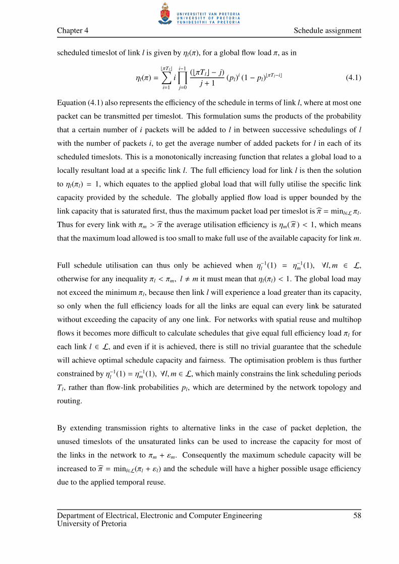
Chapter 4 Schedule assignment
scheduled timeslot of link l is given by ηl(π), for a global flow load π, as in
ηl(π) =
⌊πTl⌋∑
i=1
i
i−1∏
j=0
(⌊πTl⌋ − j)
j + 1(pl)
i (1 − pl)⌊πTl−i⌋ (4.1)
Equation (4.1) also represents the efficiency of the schedule in terms of link l, where at most one
packet can be transmitted per timeslot. This formulation sums the products of the probability
that a certain number of i packets will be added to l in between successive schedulings of l
with the number of packets i, to get the average number of added packets for l in each of its
scheduled timeslots. This is a monotonically increasing function that relates a global load to a
locally resultant load at a specific link l. The full efficiency load for link l is then the solution
to ηl(πl) = 1, which equates to the applied global load that will fully utilise the specific link
capacity provided by the schedule. The globally applied flow load is upper bounded by the
link capacity that is saturated first, thus the maximum packet load per timeslot is π = minl∈L πl.
Thus for every link with πm > π the average utilisation efficiency is ηm( π ) < 1, which means
that the maximum load allowed is too small to make full use of the available capacity for link m.
Full schedule utilisation can thus only be achieved when η−1l
(1) = η−1m (1), ∀l,m ∈ L,
otherwise for any inequality πl < πm, l , m it must mean that ηl(πl) < 1. The global load may
not exceed the minimum πl, because then link l will experience a load greater than its capacity,
so only when the full efficiency loads for all the links are equal can every link be saturated
without exceeding the capacity of any one link. For networks with spatial reuse and multihop
flows it becomes more difficult to calculate schedules that give equal full efficiency load πl for
each link l ∈ L, and even if it is achieved, there is still no trivial guarantee that the schedule
will achieve optimal schedule capacity and fairness. The optimisation problem is thus further
constrained by η−1l
(1) = η−1m (1), ∀l,m ∈ L, which mainly constrains the link scheduling periods
Tl, rather than flow-link probabilities pl, which are determined by the network topology and
routing.
By extending transmission rights to alternative links in the case of packet depletion, the
unused timeslots of the unsaturated links can be used to increase the capacity for most of
the links in the network to πm + εm. Consequently the maximum schedule capacity will be
increased to π = minl∈L(πl + εl) and the schedule will have a higher possible usage efficiency
due to the applied temporal reuse.
Department of Electrical, Electronic and Computer Engineering 58University of Pretoria

Chapter 4 Schedule assignment
4.3.3 Link-assigned TDMA with temporal reuse
The simple link-assigned TDMA schedule in Figure 4.6 can be extended with LET, which
would increase the usage efficiency and enable network coding, as shown in Figure 4.10. The
same number of timeslots is used, but now when the primary link does not have packets the
reserve links may be used. This will reduce wasted timeslots, and in addition, network coded
packets can be multicast under certain circumstances when there are additional links with
transmission rights at a node.
Timeslot 1 Timeslot 2 Timeslot 3 Timeslot 4
Timeslot 5 Timeslot 6 Timeslot 7 Timeslot 8
Figure 4.10: Link-assignment with extended transmission rights, or link-assigned TDMA with
temporal reuse.
4.3.4 Link-assigned STDMA with temporal reuse
For link-assigned STDMA shown in the example of Figure 4.7, the transmission rights of
scheduled nodes can also be extended, but because of the spatial reuse the temporal reuse will
be less than with node-assigned scheduling. The schedule with the extended transmission rights
is thus depicted in Figure 4.11, where the same number of timeslots are used as in link-assigned
STDMA.
An equivalent scenario of critical link-set fulfilment, as with node-assigned STDMA, can be
created as indicated in Figure 4.12. Comparing this compacted schedule to node-assigned
STDMA in Figure 4.9, it can be seen that the same frame-size is achieved. The spatial reuse
for node-assigned STDMA is 7/4 and the temporal reuse is 14/7 = 2, while the spatial reuse
for link-assigned STDMA with LET is 9/4 > 7/4 and the temporal reuse here is 15/9 < 2.
As expected, the spatial reuse is greater and the temporal reuse less with LET, but the same
Department of Electrical, Electronic and Computer Engineering 59University of Pretoria

Chapter 4 Schedule assignment
Timeslot 1 Timeslot 2 Timeslot 3 Timeslot 4
Timeslot 5 Timeslot 6 Timeslot 7
Figure 4.11: Link-assigned STDMA with prioritised extended transmission rights, higher
utilisation efficiency and network coding support.
number of timeslots are required.
Additional benefits may be gained with LET however, since it integrates more easily
into an optimisation framework. The integrated secondary scheduling with LET also makes
capacity estimation easier than with node-assigned scheduling, which makes LET more
appropriate for use in optimisation. In practice, the LET schedule frame in Figure 4.12 will not
be as short, but a separate timeslot will be dedicated to each link to have first priority. Such a
schedule may, or may not perform as well as a node-assigned schedule.
Timeslot 1 Timeslot 2 Timeslot 3 Timeslot 4
Figure 4.12: Compacted link-assigned STDMA with LET, catering for the critical link-set.
Department of Electrical, Electronic and Computer Engineering 60University of Pretoria

CHAPTER 5
SCHEDULE CAPACITY
One of the most important measures of network performance is schedule capacity, which is
calculated in this chapter. Having formed the network topology and the links of the wireless
mesh network, and having defined the particulars of medium access control, the transmission
scheduling needs to be optimised. The primary utility of schedule performance is the capacity
that a network can achieve under the control of the schedule. This utility serves as a metric
of comparison to evaluate the goodness of a schedule, and to facilitate in the planning of the
wireless network and its usage. Specifically, the capacity is measured as the optimal set of link
transmission rates that can be achieved, which is referred to as the link transmission capacity
or rate region of the network.
From the viewpoint of optimisation, the link rate region defines the multivariate space
that restricts the transmission rates that can be achieved by the wireless links. Since the links
of a network share the same communication medium, the achievable transmission rate of a
link depends on the transmission rates of the rest of the links, and thus forms a rate possibility
space. The rate region is then used to restrict the link transmission rates when optimising the
schedule, in terms of its spatial and temporal reuse groups and their duration in the transmission
schedule.
The link transmission rate region of link-assigned STDMA is reviewed from [32] in this
chapter, and those principles are used to formulate the temporal reuse-aware rate region
applicable to link-assigned STDMA with extended transmission rights (LET). The capacity
region formulation is then simplified and a feasible sub-optimum is obtained by relying on link
Department of Electrical, Electronic and Computer Engineering 61University of Pretoria

Chapter 5 Schedule capacity
prioritisation. This inherent secondary scheduling in LET makes capacity estimation possible,
as opposed to node-assigned scheduling where a separate definition of secondary scheduling is
required. The issues and calculations that are covered in this chapter is shown in Figure 5.1.
Schedule
capacity
Link-assigned
STDMA capacity
Capacity with
temporal reuse
Rate
region
Temporal reuse-
aware rate region
Rate region
estimation
Ordering
policy
Link rate
vectors
Figure 5.1: An outline of the topics discussed in this chapter.
5.1 LINK-ASSIGNED STDMA CAPACITY
The purpose of a transmission schedule is to control link transmission powers and rates,
regulate medium access and provide adequate capacity for all network traffic. Transmission
schedules are predetermined for a limited number of timeslots, with the frame being repeated
in time. The capacity provided during a specific timeslot is defined by the associated link rate
vector, which gives the transmission rate for each active link in the spatial reuse group, or
clique. The link rate region for link-assigned STDMA in [32] is partly reviewed in this section,
since it forms the basis of the capacity determination for link-assigned STDMA with temporal
reuse.
The target SINR for transmission at a discrete r-multiple of the base rate is given by
γ(r)tgt, where r = 1 refers to the base transmission rate and r = 0 a zero transmission rate.
In practice the transmission rate of link l is limited to cl = c(r)tgt = rW log(1 + γ
(1)tgt ) when
γ(r)tgt ≤ γl(P) < γ
(r+1)tgt , where W is the system bandwidth in the Shannon capacity formulation.
Each link can be assigned a total of rl,max + 1 different rates according to the link rate allocation
policy Cl =c
(rl)tgt : rl ∈ [0, rl,max]
, where rl = 0 means an inactive link and rl = rl,max the
maximum possible multiple of the base rate for the link l. All possible link rate vectors are
Department of Electrical, Electronic and Computer Engineering 62University of Pretoria

Chapter 5 Schedule capacity
given by
V = vk = (cl ∈ Cl : l ∈ L) , k ∈ [1,K] . (5.1)
There can be at most K = |V| ≤∏l∈L
(rl,max + 1
)unique link rate vectors, but in actuality much
less, owing to interference limiting the spatial reuse clique sizes. A schedule allocates a certain
number of timeslots to each link rate vector so that the long-term achievable link rate region can
be defined as
C = conv (V) =
c =
∑
k∈[1,K]vk∈V
αkvk
∣∣∣∣∣∣
αk ≥ 0,∑
k αk = 1,
k ∈ [1,K]
. (5.2)
This is similar to the capacity region for wireless ad hoc networks defined in [33]. The convex
hull conv() of the setV includes all achievable average link capacities owing to time-sharing of
all the link rate vectors. This convex combination of link rate vectors allocates a time fraction
of αk to every link vector vk to form the polyhedral rate region.
5.2 CAPACITY WITH TEMPORAL REUSE
Given a scheduled link rate vector vk ∈ V that experiences packet depletion for one of the
associated links L(vk) = l ∈ L : vk(l) > 0, the scheduler can resort to transmission on an
alternative link through temporal reuse. In such a timeslot where an alternate link is used,
another link rate vector vm , vk describes the capacity used for the temporal reuse instance. All
possible link rate vectors that can describe temporal reuse for the primary vector vk are defined
by the extended setV(vk) = vm ∈ V : P(vk) P(vm).
An extended set of link rate vectors can be associated with any one specific link rate
vector, such that spatial reuse is maintained but with increased temporal reuse. The node
transmission powers for a link rate vector vk are given by P(vk), and the power assignment
should not be exceeded by any alternate link rate vector.
5.2.1 Temporal reuse-aware rate region
The average link capacities used for a scheduled extended set depend on its ordering policy,
the network topology, radio propagation model and traffic load, as these factors influence the
prevalence of packet depletion. For all repetitions of a timeslot where an extended set of vk
is scheduled, a certain fraction ϕkm of repetitions will be represented by every link rate vector
Department of Electrical, Electronic and Computer Engineering 63University of Pretoria

Chapter 5 Schedule capacity
vm ∈ V(vk) in the extended set. These fractions can only be determined by simulating the
network, although the values Φ(V) = ϕkm :∑ϕkm ≤ 1, vm ∈ V(vk) : vk ∈ V will change
when a schedule is used that is optimised using those values in the temporal reuse-aware rate
region
Ce =
∑
k∈Kvk∈V
αk
∑
vm∈V(vk)
ϕkmvm
∣∣∣∣∣∣
αk ≥ 0,∑
k αk = 1,
k ∈ K
. (5.3)
The aware rate region Ce gives the achievable link capacities with the extended temporal
reuse sets when taking the inefficiencies due to packet depletion into account. Optimising a
schedule with more accurate representations of the link rate vectors leads to improved network
performance.
5.2.2 Rate region estimation
A schedule optimisation algorithm should be independent of a specific network topology and
radio propagation model, so several assumptions and simplifications are applied to create a
generic optimiser:
(i) Each alternative link in the temporal reuse set must operate at the maximum possible
transmission rate, within the power constraints.
(ii) The usage probabilities of links in a temporal reuse set are determined only on the basis
of the order in which the links are queried for packets in the case of packet depletion,
regardless of network topology or radio propagation model.
Since some links in a temporal reuse set could have sufficient SINR to transmit at different rates,
only the highest rate (primary criterion) is chosen to maximise the capacity of each extended
set. For schedules that use link rate vectors with variable power control, a minimum power
criterion (secondary with a small ǫ > 0) could also be used to differentiate between multiple
link rate vectors with a maximum rate for a specific link. The temporal reuse set for a clique
node n ∈ T (vk) = n ∈ N : L(vk) ∩ O(n) , ∅, where O(n) are the outgoing links of node n, is
thus calculated as Ln(vk) = l ∈ L : cl > 0, cl ∈ Cn(vk) where
Cn(vk) =
argvm(l) max
vm∈V(vk)
(vm(l) − ǫP(vm, n)
): l ∈ O(n)
. (5.4)
To calculate the rate region Ce a very large set of |Φ(V)| = ∑vk∈V |V(vk)| values particular
to V is needed. A network-agnostic rate region can be rendered by focusing on the usage
Department of Electrical, Electronic and Computer Engineering 64University of Pretoria

Chapter 5 Schedule capacity
probabilities of alternative links in Ln(vk), instead of alternative link rate vectors as in the case
of Φ(V). With temporal reuse, when a primary scheduled link experiences packet depletion the
alternative links are queried in a certain order for available packets, according to the ordering
policy, until a usable link is found.
Each link l in a temporal reuse set Ln(vk) is assigned an ordering value Θn(vk, l) ∈[0, |Ln(vk)| − 1], where a smaller value means a higher priority, to establish an ordering
policy, so a link l ∈ Ln(vk) with a higher priority Θn(vk, l) < Θn(vk,m) than m ∈ Ln(vk) will
have a higher usage probability Un(vk, l) > Un(vk,m). The number of usage probabilities
are reduced with the assumption that the utilisation probabilities Un(vk, l) ≈ Uo(v j,m) are
approximately equal when the usage priorities Θn(vk, l) = Θo(v j,m) are the same, regardless
of differences in networks, the extended sets, the particular node temporal reuse sets or links
in question. This simplification is made on the basis that it is the order in which links in the
temporal reuse set are checked that determines the link usage probabilities. Let U be the
simplified priority-based link usage probabilities, where the usage probability for a link with
priority θ is Uθ, then
U =
Uθ ∈ [0, 1] :∑
θ
Uθ ≤ 1, Uθ−i > Uθ, 0 ≤ i ≤ θ, ∀θ ≥ 0
. (5.5)
The primary outgoing link for a node, in other words the active link that is originally implicated
in vk, has priority θ = 0, and lower priority reserve links have higher θ values. The simplified
usage probabilities of outgoing links in the temporal reuse set for a specific node n active in vk
are given by
Un(vk) = βl : l ∈ O(n) ⊆ U. (5.6)
Although this form does not define a specific ordering policy, one based on relative traffic flow
magnitudes is presented in the following subsection. Let IL be the identity matrix in RL×L, where
IL(l) is the jth column in IL so that j is the index of link l in L. Temporal reuse link sets are
mutually exclusive, thus for any vk ∈ V the relationship ∩n∈T (vk)Ln(vk) = ∅ holds, so the usage
probability vector for a vk with temporal reuse is given by
U(vk) =∑
n∈T (vk)
∑
l∈O(n)
Un(vk, l)IL(l). (5.7)
The full link rate template for vk with temporal reuse given by C(vk) represents the
non-achievable capacity before taking the actual usage limits specified by U(vk) into account,
Department of Electrical, Electronic and Computer Engineering 65University of Pretoria

Chapter 5 Schedule capacity
as shown in
C(vk) =∑
n∈T (vk)
∑
l∈O(n)
Cn(vk, l)IL(l). (5.8)
The Hadamard (Schur) product of the usage probability estimates U(vk) and the rate template
C(vk) gives the resultant achievable capacity for vk with full temporal reuse, and so the
simplification of Ce gives the estimated achievable rate region Ce for networks with spatial
and temporal reuse, as shown in
Ce =
∑
k∈Kvk∈V
αk
(U(vk) ⊙ C(vk)
) ∣∣∣∣∣∣
αk ≥ 0,∑
k αk = 1,
k ∈ K
. (5.9)
Apart from the time-sharing coefficients αk : k ∈ K and the link rate vector power assignments
P(vk) : vk ∈ V, each schedule has to include the prioritised temporal reuse link rate sets
Θ(vk),U(vk),C(vk) : vk ∈ V associated with every active transmitter node n in the spatial
reuse node set (clique) T (vk) for every vk ∈ V. The schedule frame length is set at a minimum
of δ(L + 1) since the optimal solution involves at most L + 1 link rate vectors according to
Caratheodory’s theorem [34] (see [35]). The schedule is composed by cycling between the
involved link rate vectors until there are ⌈αkδ(L + 1)⌉ occurrences of each vector vk. A value of
δ = 3 has experimentally shown to give good results for various network sizes.
U is independent of a particular network topology or radio propagation model, and can
be determined once with the averaged values of simulations of many different networks and
used to optimise any network afterward, as done in the numerical analysis of the schedule
performance chapter. The number of utilisation probability values needed to calculate Ce is
|U | = maxn∈T (vk)
vk∈V
|Ln(vk)| ≪ |Φ(V)| . (5.10)
This estimate Ce is thus greatly simplified while maintaining the effect of temporal reuse on the
usage efficiency and achievable capacity of link-assigned schedules.
5.2.3 Ordering policy
The discriminator that is used to assign prioritiesUn(vk, l) to the alternative links in a temporal
reuse set vk is taken as the number of data flows∑
f Rl f that traverse a link l. The more flows
that have to be routed by a link, the greater the need for capacity, thus preference is given to
Department of Electrical, Electronic and Computer Engineering 66University of Pretoria

Chapter 5 Schedule capacity
links that relay more flows. This traffic flow-based ordering policy assigns higher priority to the
higher traffic link as formulated by
sgn(Un(vk, l) −Un(vk,m)
)=
+1 when∑
f Rl f >∑
f Rm f ,
0 never,
−1 when∑
f Rl f ≤∑
f Rm f
for l , m, ∀l,m ∈ O(n), ∀n ∈ T (vk). (5.11)
This policy check is performed for every pair combination of the outgoing links of a scheduled
node n in a temporal reuse set vk.
Department of Electrical, Electronic and Computer Engineering 67University of Pretoria

CHAPTER 6
SCHEDULE OPTIMISATION
Quality of service and the efficient use of communication resources necessitate engineered
optimisation of the control processes of the wireless mesh network. The fairness between
the flow rates is an important measure of service quality, and a good schedule should give
preference to flow rate fairness over total network throughput. Specifically, a global utility of
proportional fairness is used in this work to evaluate the fitness of a candidate transmission
schedule, with the flow rates limited by the link capacities. In Chapter 5 the capacity of all
possible spatial and temporal reuse groups were determined, and those capacities will be used
here to help construct an optimal schedule.
The fractional duration of each reuse group is modified to bring about a change in the
link rate region of the network, guided by the proportionally fair objective function. Since the
fractional durations of all the reuse groups should sum to 1, the rate region is called convex
and it limits the total flow loads that can traverse the links. The resulting problem is thus
termed convex optimisation, where a linear objective function is subject to a convex constraint.
Solving the convex optimisation problem produces the optimal flow rates and perceived link
demands, which indicate capacity shortages in some links. The duration of a reuse group
that can fulfil the largest sum of demands is then increased, until the maximum utility is reached.
Convex optimisation for link-assigned STDMA is first reviewed, and the computational
aspects of the solution are discussed. The optimisation problem is then extended to address
link-assigned STDMA with extended transmission rights, by using the modified temporal
reuse-aware capacity region calculated in Chapter 5. Complexity reductions are introduced
Department of Electrical, Electronic and Computer Engineering 68University of Pretoria

Chapter 6 Schedule optimisation
to make the temporal reuse-aware solution computationally feasible, and the solver is further
explained. This chapter then endeavours to derive the complete optimised transmission
schedule for networks running LET. An outline of the topics that are discussed in this chapter
is given in Figure 6.1.
Schedule
optimisation
Link-assigned
STDMA
optimisation
Column
generation
approach
Main
algorithm
Scheduling
subproblem
Networking
subproblem
Figure 6.1: The schedule optimisation topics covered in this chapter.
6.1 LINK-ASSIGNED STDMA OPTIMISATION
Link capacities are represented by the transmission schedule, which can be optimised to
maximise a global utility function. The level of satisfaction with a flow rate s f is given by
a utility function u(s f ), which is concave and strictly increasing. Maximising the weighted
network throughput∑
f∈F w f s f leads to grossly unfair flow rates [36], so a proportionally fair
flow utility is decided on where u → −∞ when s f → 0+. The flow rates s are proportionally
fair if, and only if, u(s f ) = log(s f ) (see [37]), and this leads to a higher total network throughput
than with maximisation of a uniform flow rate.
Network throughput depends on the available link capacities, which are consumed with
relaying potentially multiple flows. The aggregate traffic load on the links is given by the
vector Rs, which is due to the point-to-point data flows and the multihop nature of the mesh
network. The achievable link rates are given by the capacity vector c ∈ C, so that the flow rates
are limited by the primary constraint Rs c, where denotes a component-wise inequality.
The purpose of the optimisation problem is to find the time-sharing coefficients αk : k ∈ K
Department of Electrical, Electronic and Computer Engineering 69University of Pretoria

Chapter 6 Schedule optimisation
(let K = [1,K]) for a capacity vector c that maximises the global utility according to
maximise∑
f u(s f
)
subject to Rs c
c ∈ C, s 0.
(6.1)
The concave global utility proposed in [32] is subject to convex constraints so it can be solved
as a convex optimisation problem that produces a cross-layer optimised solution. The resultant
schedule consists of link rate vectors vk : k ∈ K and the associated time-sharing coefficients
αk : k ∈ K, which define transmission power and rate control in the physical layer and
medium access control in the data link layer, respectively. The delivery route of each data flow
is established in the network layer as represented by R, and the flow rates s are regulated in the
transport layer.
The optimal solution involves at most L + 1 link rate vectors according to Caratheodory’s
theorem [34] (see [35]), therefore there are at most L + 1 non-zero αk values in the optimal
schedule. The exact number of utilised link rate vectors depends on the specific optimal
solution for a particular network. The greater the number of links, the more numerous the
possible spatial reuse groups, which increases the number of used link rate vectors. For a
proper TDMA (time-division multiple access) schedule, it can be seen that L link rate vectors
would be needed for a feasible solution. When spatial reuse comes into play, less link rate
vectors can describe the same capacity of TDMA, so the limit of the number of involved link
rate vectors is not exceeded.
6.2 COLUMN GENERATION APPROACH
The global utility maximisation problem in Equation (6.1) determines the time-sharing
coefficients for each link rate vector in V. The number of link rate vectors is exponential in
the number of network links, so calculating and storing them in order to solve Equation (6.1)
becomes a hurdle as the network grows. The solution also tends to be more inaccurate with
computer solvers when more link rate vectors are involved.
For these reasons the mathematical programming technique of column generation [38] is
employed, where modifications specific to temporal reuse are made to the algorithm discussed
in [32] and [39], which is reconsidered in this section. Optimisation can then be started with
Department of Electrical, Electronic and Computer Engineering 70University of Pretoria

Chapter 6 Schedule optimisation
only a small number of link rate vectors, and more vectors that contribute most to increasing
the global utility are added through column generation. The process of optimising a schedule
with column generation, for networks that employ both spatial and temporal reuse, is explained
in this section.
6.2.1 Main algorithm
The utility maximisation problem guides the column generation by providing information
pertaining to capacity demands, therefore it is referred to as the master problem. The full
master problem in Equation (6.1) contains all K link rate vectors, but it is restricted to a subset
J ⊆ K of vectors in the restricted master problem (6.2) used for column generation. The full
master problem is described by
maximize∑
f u(s f
)
subject to Rs c, s 0
c =∑
k∈J⊆Kvk∈V
αk
(U(vk) ⊙ C(vk)
)
∑k αk = 1, αk ≥ 0, k ∈ J ⊆ K .
(6.2)
The link-flow incidence matrix is given by R and the flow rate vector is given by s, so that Rs
gives the link flow load vector that needs to be less than the available link capacity vector c.
The available capacity is calculated according to the temporal reuse-aware link rate region.
When solving the restricted master problem the capacity demand ξl for each link l can be
determined, which indicates the relative utility improvement for a unit increase in link capacity.
For u(·) = log(·) each link demand also equals the inverse flow rate of the flow that only uses
the corresponding link [40]. These capacity demands are given by the Lagrangian duality for
(6.2), which is as follows:
L(s, c, ξ) =∑
f u(s f
)− ξT (c − Rs) . (6.3)
The optimal Lagrangian multipliers ξ∗ are used to updateJ by maximising the upper bound on
the optimum (weak duality, see [32]) according to
uu = sups0
∑f u
(s f
)− ξ∗T Rs
+ sup
c∈Ce
ξ∗T c
. (6.4)
The lower bound (6.5) involves only the columns generated thus far, as indicated by J , to find
the best supply vector. The lower bound is given by
ul = sups0
∑f u
(s f
)− ξ∗T Rs
+ sup
c∈CJe
ξ∗T c
. (6.5)
Department of Electrical, Electronic and Computer Engineering 71University of Pretoria

Chapter 6 Schedule optimisation
Finding a new link rate vector from the K-element rate region Ce that maximises capacity for
the given demand solves the scheduling subproblem supc∈Ce
ξ∗T c
. An extreme point in Ce will
maximise capacity [32] rather than a combination of link rate vectors. This generated column
does not require that all K elements have to be known, but the new vector can be obtained by
solving a mixed integer linear programming formulation discussed in the proceeding subsection.
Optimality is reached when the new link rate vector cannot supply a greater capacity
than an existing vector. The process of solving the restricted master problem and expanding
J is continued until the difference between the optimal upper bound uu and lower bound ul
becomes smaller than a certain threshold ε, as shown by
uu − ul = supc∈Ce
ξ∗T c
− sup
c∈CJe
ξ∗T c
< ε. (6.6)
The main column generation algorithm that is used to optimise a schedule, by forming J to
maximize the global utility, is as follows:
1. Initialise the index set J with the link rate vectors that correspond to a simple TDMA
link-assigned schedule operating at base rates only, with no spatial reuse.
2. Solve the restricted master problem to optimality with a primal-dual interior-point method
[41] to obtain the optimal Lagrangian multipliers or capacity demands ξ∗.
3. Add the new link rate vector, that solves the scheduling subproblem, to J .
4. Repeat the process until uu − ul < ε, or when the generated column is already present in
J .
6.2.2 Scheduling subproblem
The optimal Lagrangian multipliers ξ∗l
give the sensitivity of the lower optimum bound ul at the
optimal point c∗. By satisfying the links with the greatest demand for capacity as indicated by
ξ∗l, the lower bound can be improved most. By finding an extreme vertex in c ∈ Ce to maximise
ξ∗Tl
c a new scheduling element is added to increase the network utility. This is termed the
scheduling subproblem and for networks with temporal reuse it is formulated as finding
maxvk∈V
(ξ∗Tl
∑
n∈T (vk)
∑
l∈O(n)
Un(vk, l)Cn(vk, l)IL(l)). (6.7)
Department of Electrical, Electronic and Computer Engineering 72University of Pretoria

Chapter 6 Schedule optimisation
A mixed integer linear program is used to determine which spatial reuse clique with extended
transmission rights solves the scheduling subproblem. Let the binary variable x(r)
lindicate
whether link l is operating at r times the base rate, then the relevant constraint for all the network
links L is given by
x(r)
l∈ 0, 1, ∀l ∈ L,∀r. (6.8)
The binary variable yn specifies whether node n is transmitting or not, so the following definition
is included for all the network nodesN :
yn ∈ 0, 1, ∀n ∈ N . (6.9)
Whenever a link is transmitting at a non-zero rate the associated node also has to be activated,
so this relationship is formulated as
∑r x
(r)
l= ytr(l), ∀l ∈ L. (6.10)
In the program the instantaneous maximum transmission power of a node n is given by Pn which
is limited to a maximum as shown in
0 ≤ Pn ≤ Pmax, ∀n ∈ N . (6.11)
To ensure that all transmitting links have a sufficiently large SINR, the following linear
constraint is imposed:
M(r)
l
(1 − x
(r)
l
)+ Qtr(l)re(l)Ptr(l)x
(r)
l≥ γ(r)
tgt
(σre(l) +
∑n,tr(l)Qnre(l)Pnyn
), ∀l ∈ L,∀r. (6.12)
When a link l is transmitting then the term(1 − x
(r)
l
)becomes zero, and when the link is not
transmitting then the coefficient M(r)
lsimply ensures that the constraint is met for the linear
program to function correctly. By choosing a sufficiently large M(r)
lthe above constraint will be
met when the link is not transmitting, so the following value will suffice:
M(r)
l= Qtr(l)re(l)Ptr(l) + γ
(r)tgt
(σre(l) +
∑n,tr(l)Qnre(l)Pn
), ∀l ∈ L,∀r. (6.13)
For scheduling with fixed power the node transmit powers are fixed at Pn = Pmax, ∀n ∈ N , and
for non-adaptive rate scheduling the rate is limited to r ∈ 0, 1. The variable rate and power
mixed integer linear program considers all the possible temporal reuse priority policies, and
given the optimal Lagrangian multipliers the program is formulated as
maximise∑
n∈N∑
l∈O(n) ξlβl
∑r c
(r)tgt x
(r)
l
subject to βl : l ∈ O(n) ⊆ U, ∀n ∈ N(6.8), (6.9), (6.10), (6.11), (6.12), (6.13).
Department of Electrical, Electronic and Computer Engineering 73University of Pretoria

Chapter 6 Schedule optimisation
By ensuring that the links with greater traffic flow∑
f Rl f loads are assigned higher rates r in
a temporal reuse link set, the complexity can be reduced. The complexity of the scheduling
subproblem, however, still remains NP-hard. The following constraint can be added to the
linear program to achieve the complexity reduction:
sgn(∑rmax
r=a x(r)
l−∑rmax
r=a x(r)m
)=
+1 when∑
f Rl f ≥∑
f Rm f ,
0 when∑
f Rl f =∑
f Rm f ,
−1 when∑
f Rl f ≤∑
f Rm f
for l , m, ∀l,m ∈ O(n), ∀n ∈ T (vk), a ∈ [1, rmax]. (6.14)
This constraint guides the selection of link rates such that higher traffic links will have an equal
or higher rate than a lower traffic link in the same temporal reuse set. A lower traffic link will
thus never have a higher rate than a link with a greater flow load in the same temporal reuse set.
Department of Electrical, Electronic and Computer Engineering 74University of Pretoria

CHAPTER 7
SCHEDULEPERFORMANCE
The performance of link-assigned STDMA with extended transmission rights is measured in
this chapter, and the benefits of the temporal reuse-aware rate region are clarified. The purpose
of extending transmission rights in link-assigned scheduling is two-fold. Firstly, the increased
temporal reuse improves predefined schedule usage efficiency, and secondly, it permits network
coding that would otherwise not be possible. Having determined the added capacity with
temporal reuse, and having optimised a transmission schedule using the temporal reuse-aware
capacity, the performance of the resulting schedule needs to confirm the design goals. The
schedule performance is a function of the schedule capacity, fairness and power efficiency, and
is compared for a multitude of relevant schedules to indicate the various niche performance
areas of each schedule.
The schedule capacity is simply the maximum uniform network load while keeping the
maximum end-to-end packet delay bounded. Schedule fairness is gauged as the variance in
flow loads at the maximum schedule capacity, while the power efficiency measurements pertain
to the average transmitter powers used by a network over several runs of a scheduling frame.
These measures track key performance metrics that summarise the goodness of each scheduling
algorithm through realistic simulation, and they are thus used to present the main results of
this dissertation. Since full wireless mesh network simulations are used, the aptitude of each
scheduling algorithm can be accurately monitored in the presence of network coding additions
and the occurrence of packet depletion.
Extensive simulation was conducted to evaluate the performance of Ce-schedules optimised
Department of Electrical, Electronic and Computer Engineering 75University of Pretoria

Chapter 7 Schedule performance
Schedule
performance
Schedule
capacity
Flow rate
fairness
Transmit power
efficiency
Improvements
with temporal
reuse
Simulation
model
Estimation
of usage
efficiency
Convergence
of the master
problem
Schedule
performance
comparison
Spatial and
temporal reuse
Figure 7.1: Chapter outline for the schedule performance study.
in the temporal reuse-aware rate region as compared to C-schedules optimised in the default
non-aware rate region. The simulation model is expounded on and results are included that show
the improvements that are gained with the addition of temporal reuse. The usage probability
vector U is estimated through simulation and the process is explained and values given for
networks with differing rate/power adaptivity. Schedule performance is gauged according to
schedule capacity, fairness and power efficiency, and in this section the benefits of the temporal
reuse-aware rate region is made clear. Finally, the relationship between spatial and temporal
reuse for the various schedules is investigated. An outline of this chapter is depicted in Figure
7.1.
7.1 SIMULATION MODEL
A radio link model is used where nodes transmit omnidirectionally at a maximum
possible instantaneous power of 0.1 W and experience background receiver noise power
of σ = 3.34 × 10⁻¹² W, where an absolute circuitry temperature of 290 K and a noise figure
of 10 are assumed. The deterministic fading model Qnm = 10−4d−3nm is used with a path loss
exponent of χ = 3, transmitter and receiver gains of 1 and a 1 m reference path loss ratio of
Knm = 10−4. The threshold SINR for base rate transmission is set at γ(1)tgt = 10 dB and a shared
bandwidth of W = 83.5 MHz is used. This model corresponds broadly to that of an indoor
wireless LAN (local area network) using the entire 2.4-2.4835 GHz ISM (industrial, scientific
and medical) band.
Department of Electrical, Electronic and Computer Engineering 76University of Pretoria

Chapter 7 Schedule performance
Multihop wireless mesh networks of 10 to 30 nodes are randomly generated in two dimensions
where the maximum length of each dimension for 10, 15, 20, 25 and 30 node networks are
set at 140 m, 160 m, 180 m, 200 m and 220 m respectively. The various square dimensions
have been experimentally chosen to produce fully connected networks with a good average
spatial reuse potential that increases as the number of nodes increases. Single-path minimum
hop routing is used according to Dijkstra’s algorithm and only networks with paths between
every node pair are considered. For each data point in the results the averaged outcomes of 120
random networks are taken and each network size is analysed separately.
Schedules are determined centrally and shared with all nodes, and with the assumption
of perfect synchronisation each node can operate according to the same schedule. Each
data flow is communicated with packets where each packet can be relayed over one hop in
one timeslot when transmitting at the base rate. The schedule capacity is determined as the
maximum number of packets π that can be added per timeslot to a flow randomly chosen
according to a uniform distribution, such that the mean end-to-end packet delays are bounded.
The numerical analysis determines the mean end-to-end packet delays, the mean flow rates
and their standard deviation, and the mean transmission power per packet for the networks
operating at maximum schedule capacity.
The analyses with NC use opportunistic two-way network coding [8] where a relay node
XORs two packets intended for exchange between two neighbouring nodes. Neighbouring
nodes do not need to communicate which packets each received, neither is opportunistic
listening required with two-way coding, and the throughput gain with n-way coding is
maximised when n = 2. First-in-first-out (FIFO) transmit buffers are employed and with NC
the buffer is checked in a FIFO manner to obtain the first two packets that can be coded and
transmitted over the scheduled temporal reuse set.
7.2 IMPROVEMENTS WITH TEMPORAL REUSE
The effect of temporal reuse on schedule capacity is determined for schedules optimised in the
unaware rate region C with transmission rights extended afterwards. This C-optimisation does
not consider the capacity changes that extended transmission rights cause and is thus temporal
reuse-unaware. Every link rate vector vk that is activated in a C-schedule has transmission rights
Department of Electrical, Electronic and Computer Engineering 77University of Pretoria

Chapter 7 Schedule performance
extended to |Ln(vk)| − 1 = q − 1 alternative links for q > 0 to see what improvements in the
schedule capacity results.
2 4 6 8 10 12
0.3
0.35
0.4
0.45
0.5
(a) Temporal reuse [nodes]
Schedule
capacity [packets
/tim
eslo
t] (Pmax
=100 mW, K=1−4
, α=3, σ=3.34−12
)
2 4 6 8 10 12
100
150
200
250
300
350
400
450
(b) Temporal reuse [nodes]Schedule
packet dela
y [tim
eslo
ts/p
acket]
CVXOPT−LET [10 nodes]
CVXOPT−LET [15 nodes]
CVXOPT−LET [20 nodes]
CVXOPT−LET [25 nodes]
CVXOPT−LET [30 nodes]
Figure 7.2: Schedule capacity (a) with extended transmission rights and corresponding mean
end-to-end packet delays (b).
As the number of alternative links are increased, the schedule capacity π also increases,
as shown in Figure 7.2(a). So as transmission rights are extended, the added capacity
minl∈L εl(q + n) > minl∈L εl(q) expands for n > 0, where εl is a function of q, with greater
improvements seen for smaller network sizes owing to smaller spatial reuse and thus better
temporal reuse. The data population sizes for the large-extreme end of the x-axis are much
smaller, since not all networks can achieve such large temporal reuse. This data population size
inequality and the trade-off between the schedule capacity and end-to-end packet delays cause
the reverse trend in the packet delay values at a large temporal reuse.
The schedule optimised in the convex rate region C is named CVXOPT-LET in Figure
7.2, where LET refers to link-assignment with extended transmission rights (full temporal
reuse). The mean end-to-end packet delays for the schedule operating at capacity are given in
Figure 7.2(b) and are reduced for most of the rights extension. Thus both the schedule capacity
and the average end-to-end packet delays can be improved with temporal reuse.
Department of Electrical, Electronic and Computer Engineering 78University of Pretoria
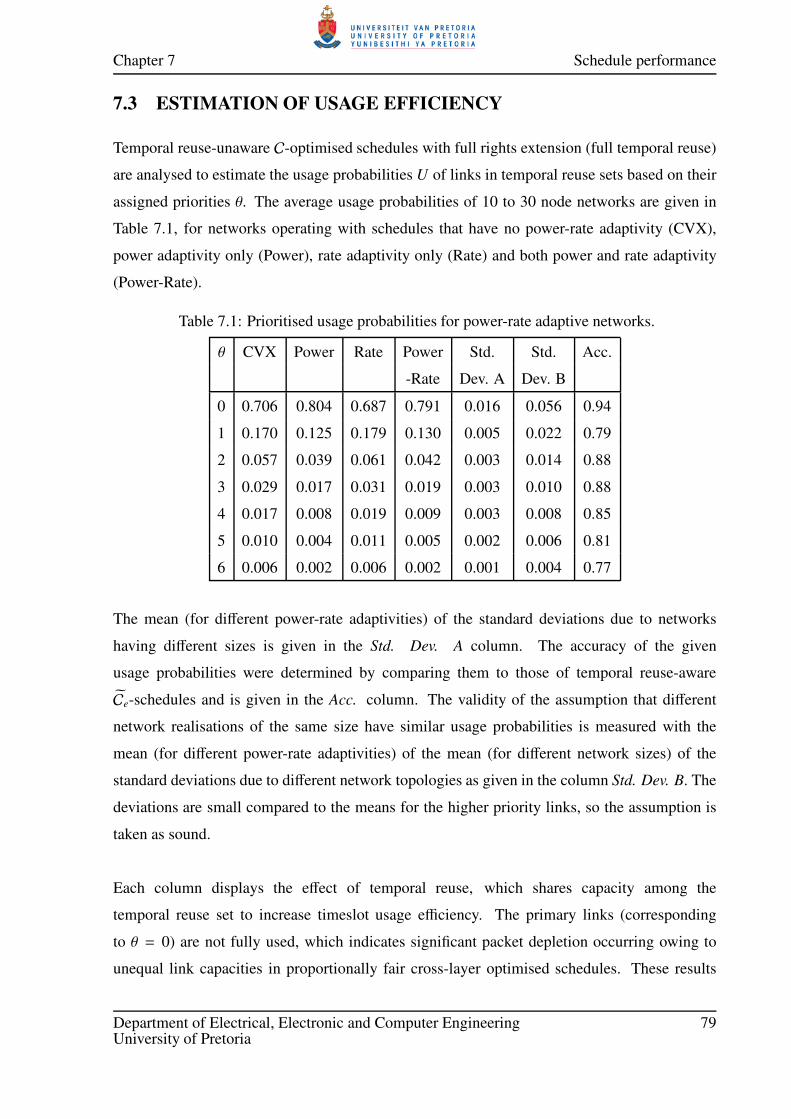
Chapter 7 Schedule performance
7.3 ESTIMATION OF USAGE EFFICIENCY
Temporal reuse-unaware C-optimised schedules with full rights extension (full temporal reuse)
are analysed to estimate the usage probabilities U of links in temporal reuse sets based on their
assigned priorities θ. The average usage probabilities of 10 to 30 node networks are given in
Table 7.1, for networks operating with schedules that have no power-rate adaptivity (CVX),
power adaptivity only (Power), rate adaptivity only (Rate) and both power and rate adaptivity
(Power-Rate).
Table 7.1: Prioritised usage probabilities for power-rate adaptive networks.
θ CVX Power Rate Power Std. Std. Acc.
-Rate Dev. A Dev. B
0 0.706 0.804 0.687 0.791 0.016 0.056 0.94
1 0.170 0.125 0.179 0.130 0.005 0.022 0.79
2 0.057 0.039 0.061 0.042 0.003 0.014 0.88
3 0.029 0.017 0.031 0.019 0.003 0.010 0.88
4 0.017 0.008 0.019 0.009 0.003 0.008 0.85
5 0.010 0.004 0.011 0.005 0.002 0.006 0.81
6 0.006 0.002 0.006 0.002 0.001 0.004 0.77
The mean (for different power-rate adaptivities) of the standard deviations due to networks
having different sizes is given in the Std. Dev. A column. The accuracy of the given
usage probabilities were determined by comparing them to those of temporal reuse-aware
Ce-schedules and is given in the Acc. column. The validity of the assumption that different
network realisations of the same size have similar usage probabilities is measured with the
mean (for different power-rate adaptivities) of the mean (for different network sizes) of the
standard deviations due to different network topologies as given in the column Std. Dev. B. The
deviations are small compared to the means for the higher priority links, so the assumption is
taken as sound.
Each column displays the effect of temporal reuse, which shares capacity among the
temporal reuse set to increase timeslot usage efficiency. The primary links (corresponding
to θ = 0) are not fully used, which indicates significant packet depletion occurring owing to
unequal link capacities in proportionally fair cross-layer optimised schedules. These results
Department of Electrical, Electronic and Computer Engineering 79University of Pretoria

Chapter 7 Schedule performance
therefore show the important benefits that can be derived from temporal reuse.
7.4 CONVERGENCE OF THE MASTER PROBLEM
The number of spatial reuse groups is limited for size-constrained fixed-topology networks,
and the resulting link rate vectors are all determined. The accurate temporal reuse-aware
link rate vectors are also determinable and the number of vectors remains the same. The
column generation must therefore end, since the number of link rate vectors is limited. Due
to Caratheodory’s theorem there is a high probability that the master problem will converge
before all the link rate vectors have been generated. The moment no new link rate vector can
increase the capacity supply, the column generation converges.
Slater’s condition is met for fully connected networks, since there is a strictly feasible
solution for the master problem. One such solution is given by a simple link-assigned TDMA
schedule that supplies a non-zero positive capacity cl for each link l in the network. The
network is fully connected therefore a non-zero positive flow rate sp can be achieved by every
flow p in the network, and if a flow rate of minl
cl/
∑p rlp
is assigned to each flow, then the
convex constraint Rs c is met. Since Slater’s condition is met strong duality holds, and there
is thus no duality gap. This means that the column generation must converge.
The convergence of the column generation for the temporal reuse-aware Ce-schedule
with extended transmission rights is depicted in Figure 7.3. The reduction in the difference
between the lower and upper bounds of the master problem is shown for different network
sizes. The mean convergence rate was measured for 120 random network realisations, for
each network size. Since larger networks have more spatial reuse groups and data flows, the
convergence rates are higher and the difference between the bounds is greater. The absence of
the duality gap is confirmed, since all of the solutions converge with zero difference between
the lower and upper bounds.
7.5 SCHEDULE PERFORMANCE COMPARISON
The practical superiority of schedule optimisation in the temporal reuse-aware rate region
is proven through measurements of schedule capacity, flow rate fairness and transmit power
Department of Electrical, Electronic and Computer Engineering 80University of Pretoria

Chapter 7 Schedule performance
0 20 40 60 80 100 120 140 160 180 2000
1000
2000
3000
4000
5000
Iterations ENIPS EHT NI SI DOG − ADNANAGOY
uu−
ul
10 nodes15 nodes20 nodes25 nodes30 nodes
Figure 7.3: Convergence of the column generation approach to schedule optimisation.
efficiency.
7.5.1 Schedule capacity
Schedule capacity is taken as the primary schedule performance measure and it is the
maximum number of packets per timeslot that can be added to a random flow so that the
schedule maintains a limited mean end-to-end packet delay. The C-schedule (CVX) capacity
is increased with extended transmission rights (CVX-LET) and when network coding is used
(CVX-LET-NC) the capacity is increased even further, as shown in Figure 7.4(a). The temporal
reuse-aware Ce-schedule with extended transmission rights (CVXAware) has greater capacity
than with CVX-LET, and the capacity improvement with NC (CVXAware-NC) is also notably
larger than with CVX-LET-NC. The temporal reuse-aware rate region gives greater capacity
to link rate vectors with good temporal reuse, which provides more NC opportunities for the
Ce-schedule.
Reference graphs include those of TDMA, STDMA, traffic-adaptive STDMA with temporal
reuse and NC (STDMA-Adaptive-LET-NC), and traffic-adaptive node-assigned schedules with
NC (Node-Assigned-NC). The STDMA schedule uses a packing heuristic [29], which packs
as many links as have not yet transmitted into a timeslot, and the traffic-adaptive STDMA
schedule is generated according to [30]. The node-assigned schedule lets a node choose a link
with probability proportional to the number of flows that traverse the link, to achieve traffic
adaptivity.
Department of Electrical, Electronic and Computer Engineering 81University of Pretoria

Chapter 7 Schedule performance
The mean end-to-end packet delays for the different schedules operating at their respective
maximum capacities are given in Figure 7.4(b). Node-assigned schedules have the lowest
delay, although they do not have the capacity of the cross-layer optimised link-assigned
schedules. The C-schedule (CVX) achieves lower delays when temporal reuse (CVX-LET) is
enabled, even though the delays for CVX are taken at a smaller load. The timeslot duration
is a function of the packet length, which affects the quality of service if the packet delays
grow large. Although, apart from the proportional fairness, the end-to-end packet delays are
allowed to grow as large as possible while remaining bounded. This is warranted to obtain the
maximum schedule capacity, which is a more important metric in this study than a secondary
quality of service concern.
10 15 20 25 300.1
0.2
0.3
0.4
0.5
(a) Network size [number of nodes]
Thro
ughput [p
ackets
/tim
eslo
t]
10 15 20 25 300
100
200
300
400
500
(b) Network size [number of nodes]
Dela
y [tim
eslo
ts/p
acket]
CVXCVX−LETCVX−LET−NCCVXAwareCVXAware−NC
TDMASTDMASTDMA−Adaptive−LET−NCNode−Assigned−NC
Figure 7.4: Schedule capacity (a) and corresponding end-to-end packet delay (b) comparisons.
The effect of rate and power adaptivity on the capacity of the cross-layer optimised
schedules is shown in Figure 7.5. Schedules with power adaptivity (CVX-Power-LET,
CVX-RatePower-LET, CVXAware-Power, CVXAware-RatePower) perform better because of
more diverse spatial reuse considerations during optimisation. When NC is enabled for the
temporal reuse-aware schedules (CVXAware), greater capacity increases are seen than with the
C-schedules, as shown in Figure 7.5(b).
Department of Electrical, Electronic and Computer Engineering 82University of Pretoria

Chapter 7 Schedule performance
10 15 20 25
0.35
0.4
0.45
0.5
(a) Network size [number of nodes]
Schedule
capacity [packets
/tim
eslo
t]
10 15 20 25
0.35
0.4
0.45
0.5
(b) Network size [number of nodes]
Schedule
capacity [packets
/tim
eslo
t]
CVX−LETCVX−Power−LETCVX−Rate−LETCVX−RatePower−LETCVXAwareCVXAware−PowerCVXAware−RateCVXAware−RatePower
CVX−LET−NCCVX−Power−LET−NCCVX−Rate−LET−NCCVX−RatePower−LET−NCCVXAware−NCCVXAware−Power−NCCVXAware−Rate−NCCVXAware−RatePower−NC
Figure 7.5: Schedule capacity comparison with (b) and without (a) NC.
10 15 20 25 300
0.01
0.02
0.03
0.04
0.05
0.06
0.07
(a) Network size [number of nodes]
Mean flo
w r
ate
[packets
/tim
eslo
t]
TDMASTDMASTDMA−Adaptive−LET−NCNode−Assigned−NC
10 15 20 25 300
0.01
0.02
0.03
0.04
0.05
0.06
(b) Network size [number of nodes]
Flo
w r
ate
Std
. D
ev. [p
ackets
/tim
eslo
t]
CVXCVX−LETCVX−LET−NCCVXAwareCVXAware−NC
Figure 7.6: Mean flow rate (a) and fairness (b) comparison.
Department of Electrical, Electronic and Computer Engineering 83University of Pretoria

Chapter 7 Schedule performance
7.5.2 Flow rate fairness
The second important schedule performance measure is flow rate fairness, which indicates
the quality of service level that can be expected with a schedule. For the schedules operating
at maximum capacity the associated mean flow rates are compared in Figure 7.6(a), where
node-assigned schedules have the highest rate and CVX the lowest. Node-assigned schedules
achieve the highest mean flow rate at the expense of rate fairness, and the best fairness is
achieved by CVX as measured by the flow rate standard deviations in Figure 7.6(b). The sum
of the logarithms of the achieved flow rates during network simulation can also be used to
assess proportional fairness, but the standard deviation of the achieved flow rates is calculated
instead to accompany the mean achieved flow rate. The temporal reuse-aware schedule
(CVXAware) achieves a better fairness than the unaware (CVX-LET) schedule, and fairness is
not compromised with the use of NC for the CVXAware schedule.
For the rate-power adaptive schedules, significantly lower flow rate deviation occurs with the
temporal reuse-aware schedules than with the unaware schedules, since the proportionally
fair global utility is more accurately determined when taking the benefits of temporal reuse
into account. The improved fairness with the Ce-schedules is especially apparent with the
power-adaptive schedules as shown in Figure 7.7(b).
10 15 20 25
0.01
0.02
0.03
(a) Network size [number of nodes]
Mean flo
w r
ate
[packets
/tim
eslo
t]
10 15 20 25
0.01
0.02
0.03
0.04
0.05
(b) Network size [number of nodes]
Flo
w r
ate
Std
. D
ev. [p
ackets
/tim
eslo
t]
CVXAwareCVXAware−PowerCVXAware−RateCVXAware−RatePower
CVX−LETCVX−Power−LETCVX−Rate−LETCVX−RatePower−LET
Figure 7.7: Mean flow rate (a) and fairness (b) comparison with variable rate and power control.
Department of Electrical, Electronic and Computer Engineering 84University of Pretoria

Chapter 7 Schedule performance
A network routes most of its data flows through the center of the network, so by giving a
centralised link more capacity there can be more flows enjoying a higher transmission rate.
This may increase the mean flow rate at the expense of reduced fairness, due to the reduced
capacity experienced by flows routed across links on the edges of the network. A proportional
fairness utility can balance the schedule capacity and fairness objectives explicitly, as opposed
to the disregard of fairness by schedules such as node-assignment.
7.5.3 Transmit power efficiency
Power efficiency is used as the third schedule performance indicator and is related to the mean
transmit power per packet. Adaptive power assignments, multi-rate transmissions and network
coding can reduce the mean transmit power per packet of the full power case (CVX-LET) shown
in Figure 7.8. By performing network coding (CVX-LET-NC) one transmission can relay two
packets, so only half the energy is used in that case, which improves the power efficiency.
Significantly less power is used with the power-adaptive schedules, and when network coding
is used the temporal reuse-aware schedules achieve greater added efficiency than the non-aware
schedules.
10 15 20 25
0.06
0.07
0.08
0.09
0.1
(a) Network size [number of nodes]
Mean tra
nsm
it p
ow
er
[Watts/p
acket]
10 15 20 25
0.06
0.07
0.08
0.09
0.1
(b) Network size [number of nodes]
Mean tra
nsm
it p
ow
er
[Watts/p
acket]
CVX−LETCVX−Power−LETCVX−Rate−LETCVX−RatePower−LETCVXAware−PowerCVXAware−RateCVXAware−RatePower
CVX−LET−NCCVX−Power−LET−NCCVX−Rate−LET−NCCVX−RatePower−LET−NCCVXAware−Power−NCCVXAware−Rate−NCCVXAware−RatePower−NC
Figure 7.8: Mean transmit power comparison with (b) and without (a) NC.
Department of Electrical, Electronic and Computer Engineering 85University of Pretoria

Chapter 7 Schedule performance
7.6 SPATIAL AND TEMPORAL REUSE
There is a relationship between spatial and temporal reuse, since greater spatial reuse implies
greater interference and consequently smaller temporal reuse. These results are evident in
Figure 7.9, where the power-adaptive schedules have the greatest spatial reuse (a) but the
smallest temporal reuse (b). Node-assigned schedules in turn achieve the highest temporal
reuse, which reduces the spatial reuse possibilities so that these also achieve the smallest
spatial reuse. The power-adaptive Ce-schedules give greater preference to temporal reuse when
compared to the C-schedules, which have higher spatial reuse. Thus, with temporal reuse-aware
optimisation a more beneficial balance is found between spatial and temporal reuse, which
results in favourable network performance.
10 15 20 25
0.6
0.8
1
1.2
1.4
(a) Network size [number of nodes]
Ratio o
f spatial re
use to a
vera
ge h
op c
ount
10 15 20 25
3
4
5
6
7
(b) Network size [number of nodes]
Mean tem
pora
l re
use c
apacity [nodes]
STDMA−Adaptive−LETNode−AssignedCVX−LETCVX−Power−LETCVX−Rate−LET
CVX−RatePower−LETCVXAwareCVXAware−PowerCVXAware−RateCVXAware−RatePower
Figure 7.9: Spatial reuse (a) and temporal reuse capacity (b) comparison.
7.7 RESULTS SUMMARY
A generic transmission scheduling algorithm has been developed that produces predefined
link-assigned schedules that maximise schedule capacity with proportionally fair end-to-end
flow rates for stationary wireless multihop mesh networks with single-path minimum hop
routing, rate and power adaptivity, both spatial and temporal reuse and network coded
Department of Electrical, Electronic and Computer Engineering 86University of Pretoria

Chapter 7 Schedule performance
forwarding. The concept of temporal reuse is newly defined in this work, and is used to
re-evaluate the hybrid node-link assignment strategy of [1]. The schedules that can induce
packet depletion are characterised, and it is shown how such schedules can benefit from
temporal reuse.
The mesh network link rate region is refined to incorporate and account for the benefits
of temporal reuse, and this temporal reuse-aware rate region is used in an updated cross-layer
optimisation scheduling algorithm based on the work in [32]. It was experimentally shown that
the temporal reuse-aware schedules have increased schedule capacity, better flow rate fairness,
and for schedules with rate and power adaptivity, greater power efficiency than schedules
optimised in the non-aware rate region of [32]. The temporal reuse-aware schedules also
achieved a better balance between spatial and temporal reuse.
Department of Electrical, Electronic and Computer Engineering 87University of Pretoria

CHAPTER 8
FOUNTAIN CODES
The transmission scheduling has been optimised in the previous part of the document, and it
has been shown to provide improved performance. The link-assigned schedules with extended
transmission rights allow for network coding, and it is this aspect of the wireless mesh network
operation that is focussed on for the remainder of this study. The research goal is to determine
whether the integration of network coding into link channel coding and source coding can
improve the network performance. Sparse graph error-correction codes are some of the most
efficient and highest performance codes, so a subclass called fountain codes is employed
specifically due to its rateless output property.
The purpose of the error-correcting channel code is to counteract the signal distortions
caused by channel noise. Different types of channels are firstly analysed in this chapter,
to determine the effects their noise have on transmission. General sparse graph codes are
then introduced and specific subclasses such as low-density parity-check and fountain codes
are explained. The sparse graph decoding mechanism is then formulated, as it is the key
component that determines the effectivity of the channel code. This mechanism is termed
belief propagation, and its behaviour is analysed with the use of density evolution. It is shown
that density evolution is an important tool in specifically improving the structure of fountain
codes for better error-correcting performance. An outline of the chapter is given in Figure 8.1,
indicating the topics addressed regarding fountain codes.
Department of Electrical, Electronic and Computer Engineering 88University of Pretoria

Chapter 8 Fountain codes
Fountain
codes
BEC BSC Random
codesLDPC Fountain
codes
Message
node update
Check node
update
Message
passing
algorithm
Channel
modelling
Sparse graph
codes
Belief
propagation
decoding
Density
evolution
Figure 8.1: The fountain code outline covered in this chapter.
8.1 CHANNEL MODELLING
Signalling via electromagnetic waves has many benefits, such as the allowance of
communication between two points that would have difficulty connecting with wires.
These benefits of wireless connectivity are offset by the signal degradation caused by
environmental electromagnetic disturbances, receiver circuitry noise and reduced power due to
distance attenuation. When a series of signals are received and converted to binary digits, then
the noise will cause some of those bits to be in error. The randomness of the noise makes it
difficult to know which bits are incorrectly received, so a means of ensuring faultless reception
is not immediately apparent. Claude E. Shannon [42] showed that there is maximum bound
of information that can be transferred over an unreliable communication channel, termed the
channel capacity. The seminal work of Shannon ushered in the age of information theory and
it was finally clear that reliable data transmission is possible for rates arbitrarily close to the
channel capacity.
Understanding the nature of a communication channel is instrumental in modelling the
way in which it introduces errors into the received data. The error model can be used to good
effect when designing a signalling strategy that can ensure reliable transmission. Two of the
most important models are the binary erasure channel (BEC) and the binary symmetric channel
(BSC), which serve to describe a number of real world communication channels.
Department of Electrical, Electronic and Computer Engineering 89University of Pretoria

Chapter 8 Fountain codes
8.1.1 Binary erasure channel
In some packet-based networks the checksums of the received packets are verified, and if the
calculated checksum does not match the received checksum then the packet is erroneous. A
faulty packet needs to be retransmitted in that case, rather than attempting to correct it. Figure
8.2(a) is an example of a binary erasure channel with parameter ε, where a symbol is received
correctly with probability 1−ε and unknown or erased with probability ε. The value of an erased
packet or symbol is simply not known, even though the exact position of the erased symbol is.
Since there is a fraction of 1 − ε of all the received symbols that are correct, the BEC capacity
is BEC(ε) = 1 − ε if the channel parameter is ε. The BEC can be decoded in polynomial time
seeing that the decoding problem can be reduced to solving a system of equations [43].
8.1.2 Binary symmetric channel
An additive white Gaussian noise (AWGN) channel distorts the transmitted signal x at the
receiver by adding random noise e, which can change the symbol decision made on the
observed value y = x + e. For binary phase-shift keying (BPSK) enough added noise in
the right direction can flip a transmitted bit to its alternate, and given the symmetry of the
Gaussian noise the probability p of a misread symbol is equal for either a 0 or 1. The
resulting binary symmetric channel (BSC) shown in Figure 8.2(b) is more complicated than
the BEC, because the receiver does not know exactly which symbol positions were received
incorrectly. With the BEC the receiver knows which symbols are erased which simplifies the
task of error correction, whereas with the BSC the maximum likelihood decoding complexity
is NP-complete [44]. The BSC with channel parameter p receives a symbol correctly with
probability 1 − p and the channel capacity is given in Equation 8.1 in terms of the binary
entropy H2(p) = −p log2 p − (1 − p) log2(1 − p).
BSC(p) = 1 − H2(p)
= 1 + p log2 p + (1 − p) log2(1 − p)(8.1)
8.2 SPARSE GRAPH CODES
Reliable communication requires the implementation of a transmission strategy that can allow
for the determination or the correction of received symbols in the case of the BEC or BSC
respectively. A simple strategy is where transmitted data is repeated several times, so that the
Department of Electrical, Electronic and Computer Engineering 90University of Pretoria
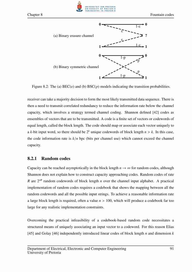
Chapter 8 Fountain codes
0
0
1
0
1
1-p
1-p
p
p
(b) Binary symmetric channel
0
1
0
1
(a) Binary erasure channel
1-0
1-0
0
?
Figure 8.2: The (a) BEC(ε) and (b) BSC(p) models indicating the transition probabilities.
receiver can take a majority decision to form the most likely transmitted data sequence. There is
then a need to transmit correlated redundancy to reduce the information rate below the channel
capacity, which involves a strategy termed channel coding. Shannon defined [42] codes as
ensembles of vectors that are to be transmitted. A code is a finite set of vectors or codewords of
equal length, called the block length. The code should map or associate each vector uniquely to
a k-bit input word, so there should be 2k unique codewords of block length n > k. In this case,
the code information rate is k/n bpc (bits per channel use) which cannot exceed the channel
capacity.
8.2.1 Random codes
Capacity can be reached asymptotically in the block length n→ ∞ for random codes, although
Shannon does not explain how to construct capacity approaching codes. Random codes of rate
R are 2nR random codewords of block length n over the channel input alphabet. A practical
implementation of random codes requires a codebook that shows the mapping between all the
random codewords and all the possible input strings. To achieve a reasonable information rate
a large block length is required, often a value n > 100, which will produce a codebook far too
large for any realistic implementation constraints.
Overcoming the practical infeasibility of a codebook-based random code necessitates a
structured means of uniquely associating an input vector to a codeword. For this reason Elias
[45] and Golay [46] independently introduced linear codes of block length n and dimension k
Department of Electrical, Electronic and Computer Engineering 91University of Pretoria

Chapter 8 Fountain codes
defined as subspaces of vector space Fn2. A linear code thus involves a basis set of k vectors of
length n to give a code rate of k/n bpc (this unit is implied for the remainder of the document).
Encoding is simplified from exponential to polynomial time with linear codes, where an input
vector (x1, . . . , xk) is uniquely mapped to a codeword by taking linear combinations of the basis
vectors identified by the coefficients x1, . . . , xk. This way an explicit codebook enumeration is
not required, as with random codes. Shannon showed [42] that there are sequences of linear
codes with rates arbitrarily close to channel capacity, so that the maximum likelihood decoding
error approaches 0 as the block length goes to infinity. Random linear codes specifically are
known to achieve capacity.
8.2.2 Low-density parity-check codes
It is clear that efficient encoding is possible with linear codes, but a practical implementation
also requires efficient decoding and a relatively good information rate. There is a need then
for capacity achieving subclasses of linear codes for which maximum likelihood decoding can
be done in polynomial time. For this reason low-density parity-check (LDPC) codes were
invented in the early 1960’s by Robert Gallager in his Ph.D dissertation [47]. LDPC codes have
fast probabilistic encoding and decoding algorithms and a wealth of analytic and combinatorial
design tools makes the codes practically and theoretically attractive.
Message
nodes
1x
2x
3x
4x
5x
6x
7x
8x
9x
10x
1 2 3 4 8 100x x x x x x
1 3 4 7 8 9 10 0x x x x x x x
2 4 6 8 0x x x x
1 5 7 8 9 100x x x x x x
3 4 5 7 90x x x x x
Check
nodes
Parity check equations
Figure 8.3: A bipartite graph representation of a linear code with parity-check equations.
LDPC codes are obtained from and decoded with bipartite graphs with n left message nodes
and r right check nodes, as shown in Figure 8.3. The code block length is n and the input
words are of length k = n − r at least. The n coordinates of the codeword vectors are associated
Department of Electrical, Electronic and Computer Engineering 92University of Pretoria

Chapter 8 Fountain codes
with the message nodes, and the codewords are chosen such that for each check node the
sum of the neighbouring message nodes are zero. The adjacency matrix of the graph is
H ∈ Fr×n2
where the entry (i, j) = 1 if the ith check node is connected to the jth message node.
Validating the parity values of a received codeword x = (x1, . . . , xn) can be done according
to HxT = 0, which will be zero if the received vector is a valid codeword. In the case of a
distorted codeword y = x + e received over an additive noise channel, the non-zero syndrome
HyT = H(x + e)T = HxT +HeT = 0+HeT = HeT = S can be computed. The decoder is tasked
with finding the most likely transmitted codeword given the observation, and the bipartite graph
is used in the process.
Any linear code has an associated representation as a bipartite graph, although the graph
is not uniquely defined by the code. The key property of LDPC codes is the sparsity of the
adjacency matrix H, which allows for algorithmic decoding efficiency. A sequence of m × n
matrices is c-sparse if mn → ∞ and the number of non-zero elements is less than c max(m, n).
For LDPC codes each adjacency matrix H has an associated generator matrix G ∈ Fk×n2
which
is used to efficiently map an input word s = (s1, . . . , sk) uniquely to a codeword x = (x1, . . . , xn)
via sG = x. The relationship between the parity-check matrix and the generator matrix is given
by HGT = 0, which produces a dense G for a sparse H. The burden of the dense generator
matrix may be offset by exploiting cyclic construction methods or other structural design
strategies to reduce the encoding complexity to an acceptable level.
The structure of LDPC bipartite graphs are often described in terms of two degree distributions
λ(x) and ρ(x), one for the message nodes and the other for the check nodes respectively. The
degree i of a message node is the number of parity-check equations in which the node features,
and a check node degree j is the number of message nodes in the associated parity-check
equation. A graph can be connected randomly and if it adheres to certain proportions of
degrees, as specified by the degree distributions, then it can form a valid decoding graph. The
fraction of graph edges that are connected to message nodes that have degree i is denoted by λi,
and the fraction of edges connected to check nodes of degree j is given by ρ j. The dual degree
Department of Electrical, Electronic and Computer Engineering 93University of Pretoria

Chapter 8 Fountain codes
distributions are thus given as in Equations (8.2) and (8.3), both from an edge perspective.
Message degree distribution: λ(x) =∑
i
λixi−1 (8.2)
Check degree distribution: ρ(x) =∑
j
ρ jxj−1 (8.3)
These degree distributions can assist in predicting the behaviour of belief propagation decoding,
as they dictate how the messages sent during decoding change after each iteration. LDPC codes
can thus be designed with optimised degree distributions so that certain performance guarantees
can be made.
8.2.3 Fountain codes
The fixed rate of LDPC codes allows for a specific code construction that fulfils certain
encoding and decoding requirements. The downside is that a different code is needed every
time the channel conditions change. For this reason, fountain codes, a rateless class of
sparse-graph codes, were designed [48, 49] for channels of which the noise level is not known
a-priori. A fountain code produces a potentially limitless stream of output symbols for a
finite given input, so that the transmitter can adaptively change the code rate if need be [50].
The key design property that makes fountain codes rateless is that every output symbol is
generated independently as the sum of a certain number of randomly chosen input symbols.
A synchronised pseudo-random number generator may be used at both the transmitter and
receiver to allow for coherent decoding of a set of received output symbols.
One of the first classes of efficient fountain codes, called LT-codes (Luby transform-codes),
was discovered by Michael Luby [48], specifically for the erasure channel. The focus in the
work on joint coding is on binary fountain codes that are truncated, since the block length can
be potentially infinite. An LT-code output symbol is also the sum of i independently chosen
input symbols, where the probability of an output node with degree i is given by Ωi. The output
degree distribution generator polynomial is Ω(x) =∑
iΩixi, which is a useful polynomial
construct that assists in calculating for example the mean output degree Ω′(1) =∑
i iΩi. An
LT-code can then be described as a fountain code with parameters (k,Ω(x)). The decoding
graph or Tanner graph for an LT-code is also a bipartite graph with k left input nodes and n
right output nodes, and the graph also serves as the direct encoding graph. In this respect the
adjacency matrix H is used differently than in an LDPC code, since a different generator matrix
Department of Electrical, Electronic and Computer Engineering 94University of Pretoria

Chapter 8 Fountain codes
is employed by an LDPC code.
LT-codes are meant to be used especially in erasure environments, such as the BEC, and
is designed to be hard-decoded without belief propagation. An output degree distribution has
been optimised for this LT-code scenario, and it is termed the robust soliton distribution [49].
This distribution is composited from two degree distributions w(d) and t(d), which are each a
function of the probabilities for a given degree d. The ideal soliton distribution is defined in
Equation (8.4), where k is the number of input nodes or source symbols.
Ideal solition distribution: w(d) =
1/k for d = 1
1/ (d(d − 1)) for 1 < d ≤ k(8.4)
The second component function is given in Equation (8.5), where S = c√
k log(k/δ), with c < 1
an arbitrary positive constant and (1−δ) the probability that all k input symbols can be recovered
when only kZ output symbols are available. The robust soliton distribution Ω(x) =∑
i µ(i)xi is
then a function of the combination of the two distributions as shown in Equation (8.6), where
Z =∑k
d=1(w(d) + t(d)).
Modifying distribution: t(d) =
S/(dk) for d = 1, 2, . . . , k/S − 1
S log(S/δ)/k for d = k/S
0 for d > k/S
(8.5)
Robust soliton distribution: µ(d) =w(d) + t(d)
Z(8.6)
The ideal soliton distribution is designed to theoretically minimise the expected overhead,
although fluctuation around the mean and lack of packet diversity can cause a deficiency
of symbols of degree one. These symbols are required for hard-decoding, so the robust
soliton distribution is modified to produce more symbols of degree one to ensure successful
decoding. The input node degree distribution Ψ(x) describes the fractions of input nodes that
have certain degrees, and since input nodes are randomly connected with an average degree of
ζ = nΩ′(1)/k it can be shown through a Taylor expansion that the input node degree distribution
is Ψ(x) = eζ(x−1).
8.2.4 Comparison between LDPC and fountain codes
Fountain codes were originally designed for efficient broadcasting of common content to many
users connected via binary erasure channels. Even when users have different symbols erased,
Department of Electrical, Electronic and Computer Engineering 95University of Pretoria

Chapter 8 Fountain codes
the extra symbols made available by the fountain code can be used by all users to get sufficient
data for lossless recovery with hard-decoding. Since fountain codes can be soft-decoded with
the means of belief propagation, it has been adapted to serve on other channels such as the BSC
or AWGN channels like LDPC codes.
Fountain codes have been designed so that it can produce a potentially endless amount
of output symbols, and is thus fully rateless. LDPC codes, on the other hand, normally have
fixed input-to-codeword rates. The performance guarantees of the LDPC code depends on the
specific rate for which its degree distributions have been optimised. For fountain codes only
the output degree distribution needs to be optimised, so that the code can still assume any rate
with the Poisson distributed input degree distribution.
LDPC codes have a separate generator matrix with which an input is transformed into a
codeword, whereas fountain codes use the parity-check matrix directly as the generator matrix
for transforming an input into an output. This means that the LDPC syndrome becomes the
fountain code output word, and the LDPC codeword corresponds with the fountain code
input word during belief propagation decoding. The LPDC message or variable nodes is thus
also the fountain code input nodes, and the LDPC check nodes is the fountain code output nodes.
The LDPC parity-check equations are calculated according to all-zero parity, while the
effective fountain code syndrome/output is not all-zero. This eases the design of fountain
codes, since there is no separate generator matrix that has to conform with the all-zero syndrome
requirement HGT = 0. Regardless of the actual syndrome value S , belief propagation remains
equally effective in solving the key equation HyT = S . Table 8.1 lists a number of important
distinctions between LDPC codes and fountain codes.
Table 8.1: A comparison of key characteristics between LDPC and fountain codes.
LDPC Fountain code
Rate Fixed Rateless
Encoding sG = x HsT = x
Decoding HxT = 0 HxT = S
Message degree distribution λ(x) ψ(x)
Check degree distribution ρ(x) ω(x)
Department of Electrical, Electronic and Computer Engineering 96University of Pretoria

Chapter 8 Fountain codes
8.3 BELIEF PROPAGATION DECODING
The decoder at the receiver-side is tasked with finding the most likely codeword that was
sent, given the information of the observed codeword. By listing all the codewords and
calculating the conditional probability for each of the codewords, given the observed values,
the codeword with the maximum probability can be found. Shannon proved [42] that the
maximum likelihood decoding error goes to zero exponentially fast with increases in the code
block length. This maximum likelihood decoding is the best the receiver can do, since it
uses all the available information to the best of its ability. Unfortunately, explicit codeword
enumeration and conditional probability calculation is prohibitively complex for practical
block lengths, so maximum likelihood decoding is not computationally feasible for most codes.
Basing a code on a graph, such as a bipartite graph for sparse graph codes, provides the
potential for elegant and efficient encoding and especially decoding algorithms. One such
decoding algorithm is belief propagation, which is a subclass of iterative message-passing
algorithms. Belief propagation is also used in artificial intelligence [51]. Belief propagation
sends sets of messages back and forth between the message and check nodes in the bipartite
graph, where the messages are beliefs or probabilities of what each node value should be. The
message sent from a message node to a directly connected check node is computed using the
observed value for the message node from the channel reception and the values received from
all the other directly connected check nodes. Note that the message computation does not take
into account the value received from the check node for which it is calculated. This condition
of not including a value from a node in a message to that node also applies for messages sent
from check to message nodes.
A bipartite coding graph establishes a relationship between the message nodes involved
in a parity-check equation, which is useful in helping to determine the value of a message
node if for example its value is erased. Furthermore, through the coordination of value
beliefs these parity-check equations can help to resolve low reliability values. It is the
structure of the sparse graph code that allows for efficient message-passing that can improve
value reliabilities. Working from the parity-check equation each check node c can inform a
message node v of the value it believes the message node should have, without consulting the
observed received value mv associated with the message node. In Figure 8.4(b) the check node
Department of Electrical, Electronic and Computer Engineering 97University of Pretoria

Chapter 8 Fountain codes
y3 = x2 + x4 + x6 + x8 calculates the perceived value my3x4of message node x4, by solving
y3 + x4 − y3 = x2 + x4 + x6 + x8 + x4 − y3. The parity-check equation is a summation in the
binary Galois field, where a subtraction is effectively an addition, so that x4 = x2 + x6 + x8 + y3.
In this manner a message node value can be calculated at an involved check node, without
requiring information from the message node in question. This is the key mechanism that
belief propagation exploits to perform error-correction.
4y
2 3x ym
6 3x ym
8 3x ym
3 4y xm
(b) Check node update
1x
2x
3x
4x
5x
6x
7x
8x
9x
10x
5y
3 2 4 6 8y x x x x
2y
1y
4xm
1 4y xm
2 4y xm
5 4y xm4 3x ym
(a) Message node update
4x 1y
2y
3y
5y
1x
2x
3x
5x
6x
7x
8x
9x
10x
4y
Figure 8.4: Belief propagation message (a) and check node (b) updates.
8.3.1 Message node update
To formulate the exact belief propagation update equations, a mechanism is firstly required to
accurately combine the channel and check node beliefs for a message node into an averaged
group belief. In the case of Figure 8.4(a) the beliefs mx4,my1x4
,my2x4,my5x4
must be aggregated
into one belief. For this purpose each belief can be expressed as a log-likelihood, and then
simply summed together to obtain the average belief. This belief (mx4y3) is then sent to the
non-participating check node to inform it of the value of the specific message node, which
can then be used in the message node update of the following iteration. The information,
previously sent from the check node to which the message node now responds, is not factored
into the update to avoid intrinsic information transfer. This is an important condition, because
if a check node receives its own information back then it fortifies its own beliefs, which is
unwarranted. This intrinsic information cycling will happen eventually, unless the bipartite
graph has no cycles and forms a tree. A cycle occurs when two or more message nodes share
two or more check nodes, which causes a vice versa situation wherein a check node’s belief is
Department of Electrical, Electronic and Computer Engineering 98University of Pretoria
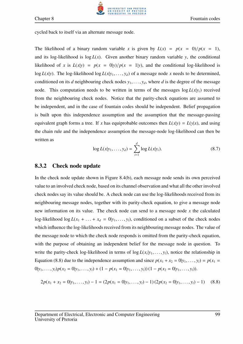
Chapter 8 Fountain codes
cycled back to itself via an alternate message node.
The likelihood of a binary random variable x is given by L(x) = p(x = 0)/p(x = 1),
and its log-likelihood is log L(x). Given another binary random variable y, the conditional
likelihood of x is L(x|y) = p(x = 0|y)/p(x = 1|y), and the conditional log-likelihood is
log L(x|y). The log-likelihood log L(x|y1, . . . , yd) of a message node x needs to be determined,
conditioned on its d neighbouring check nodes y1, . . . , yd, where d is the degree of the message
node. This computation needs to be written in terms of the messages log L(x|yi) received
from the neighbouring check nodes. Notice that the parity-check equations are assumed to
be independent, and in the case of fountain codes should be independent. Belief propagation
is built upon this independence assumption and the assumption that the message-passing
equivalent graph forms a tree. If x has equiprobable outcomes then L(x|y) = L(y|x), and using
the chain rule and the independence assumption the message-node log-likelihood can then be
written as
log L(x|y1, . . . , yd) =
d∑
i=1
log L(x|yi). (8.7)
8.3.2 Check node update
In the check node update shown in Figure 8.4(b), each message node sends its own perceived
value to an involved check node, based on its channel observation and what all the other involved
check nodes say its value should be. A check node can use the log-likelihoods received from its
neighbouring message nodes, together with its parity-check equation, to give a message node
new information on its value. The check node can send to a message node x the calculated
log-likelihood log L(x1 + . . . + xd = 0|y1, . . . , yl), conditioned on a subset of the check nodes
which influence the log-likelihoods received from its neighbouring message nodes. The value of
the message node to which the check node responds is omitted from the parity-check equation,
with the purpose of obtaining an independent belief for the message node in question. To
write the parity-check log-likelihood in terms of log L(xi |y1, . . . , yl), notice the relationship in
Equation (8.8) due to the independence assumption and since p(x1 + x2 = 0|y1, . . . , yl) = p(x1 =
0|y1, . . . , yl)p(x2 = 0|y1, . . . , yl) + (1 − p(x1 = 0|y1, . . . , yl)) (1 − p(x2 = 0|y1, . . . , yl)).
2p(x1 + x2 = 0|y1, . . . , yl) − 1 = (2p(x1 = 0|y1, . . . , yl) − 1) (2p(x2 = 0|y1, . . . , yl) − 1) (8.8)
Department of Electrical, Electronic and Computer Engineering 99University of Pretoria

Chapter 8 Fountain codes
Forming a chain rule from Equation (8.8), it can be shown that the entire parity-check
formulation can be included as follows:
2p(x1 + ... + xd = 0|y1, ..., yl) − 1 =
d∏
i=1
(2p(xi = 0|y1, . . . , yl) − 1) (8.9)
The log-likelihood based on the parity-check equation can then be written in terms of previously
received log-likelihood values log L(xi|y1, . . . , yl). First note that the definition L(x) =p(x=0)
p(x=1)of
likelihood is used to integrate Equation (8.9) into the proof so that
log L(x1 + . . . + xd = 0|y1, . . . , yl) = log
(p(x1 + ... + xd = 0|y1, ..., yl)
1 − p(x1 + ... + xd = 0|y1, ..., yl)
)
= log
(1 + (2p(x1 + ... + xd = 0|y1, ..., yl) − 1)
1 − (2p(x1 + ... + xd = 0|y1, ..., yl) − 1)
)
= log
(1 +
∏di=1 (2p(xi = 0|y1, . . . , yl) − 1)
1 −∏ℓi=1 (2p(xi = 0|y1, . . . , yl) − 1)
).
(8.10)
By using the identity 2 tanh−1 z = log(
1+z1−z
)it can then be shown that Equation (8.10) is
log
(1 +
∏di=1 (2p(xi = 0|y1, . . . , yl) − 1)
1 −∏ℓi=1 (2p(xi = 0|y1, . . . , yl) − 1)
)=2 tanh−1
d∏
i=1
(2p(xi = 0|y1, . . . , yl) − 1)
. (8.11)
Using the likelihood equality p(xi = 0|y1, . . . , yl) =L(xi=0|y1 ,...,yl)
1+L(xi=0|y1 ,...,yl)it can then be shown that
Equation (8.11) is
2 tanh−1
d∏
i=1
(2p(xi = 0|y1, . . . , yl) − 1)
=2 tanh−1
d∏
i=1
L(xi = 0|y1, . . . , yl) − 1
L(xi = 0|y1, . . . , yl) + 1
. (8.12)
Finally, the identity tanh z = e2z−1e2z+1
can be used to prove that the parity-check log-likelihood
log L(x1 + . . . + xd = 0|y1, . . . , yl) can be written in terms of the received log-likelihood values
log L(xi = 0|y1, . . . , yl) as
log L(x1 + . . . + xd = 0|y1, . . . , yl) =2 tanh−1
d∏
i=1
L(xi = 0|y1, . . . , yl) − 1
L(xi = 0|y1, . . . , yl) + 1
=2 tanh−1
d∏
i=1
tanh(0.5 log L(xi = 0|y1, . . . , yl))
.(8.13)
8.3.3 Message-passing algorithm
In round 0 of belief propagation each message node v sends its log-likelihood ratio m(0)vc
to neighbouring check nodes c based on the channel observations, which for a BSC(p)
Department of Electrical, Electronic and Computer Engineering 100University of Pretoria

Chapter 8 Fountain codes
channel would be log ((1 − p)/p). During further rounds each message node v will send its
log-likelihood ratio m(ℓ)vc conditioned on its channel observations and the beliefs of neighbouring
check nodes, without cycling back intrinsic information directly. Each check node c will send
a value m(ℓ)cv to each of its message nodes v so that their parity-check equations are fulfilled.
The belief update equations are thus given in Equations (8.14) and (8.15), and are executed
iteratively for a maximum number of iterations, or until the least reliable likelihoods exceed a
threshold.
m(ℓ)vc =
mv, if ℓ = 0,
mv +∑
c′∈Cv\cm(ℓ−1)
c′v , if ℓ ≥ 1.(8.14)
m(ℓ)cv = 2 tanh−1
∏
v′∈Vc\vtanh(
1
2m
(ℓ)
v′c)
(8.15)
With LDPC codes the received codeword is mapped to the message nodes via mv, but this differs
from a fountain code since its codeword is mapped to the check nodes instead. Where an LDPC
code uses a separate generator matrix to produce a codeword from an input source, the fountain
code uses the parity-check matrix to encode and decode. For this reason the check update
equation needs to include the received log-likelihood mc of every codeword symbol as mapped
to a check node. The message node log-likelihoods mv will in most cases then revert to zero,
unless the receiver has information of an input bias ps ,12. The message-passing algorithm
update equations for fountain codes, or LDPC codes that are used for compression, are given in
Equations (8.16) and (8.17).
m(ℓ)vc =
mv, if ℓ = 0,
mv +∑
c′∈Cv\cm(ℓ−1)
c′v , if ℓ ≥ 1.(8.16)
m(ℓ)cv = 2 tanh−1
tanh(1
2mc)
∏
v′∈Vc\vtanh(
1
2m
(ℓ)
v′c)
(8.17)
In the Equations of (8.14) and (8.15) the set of check nodes incident to message node v is Cv,
and the set of message nodes incident to check node c is given by Vc. In belief propagation each
graph edge is traversed a constant number of times for a constant number of belief propagation
iterations, which makes the number of operations linear in the number of message nodes for
a sparse graph. The algorithm is independent of the channel and the specific messages passed
is dependent on the channel. The benefit of belief propagation is mainly its efficiency, since
maximum likelihood decoding can be more optimal as in the case of biregular bipartite graphs
of a large common message node degree.
Department of Electrical, Electronic and Computer Engineering 101University of Pretoria

Chapter 8 Fountain codes
8.4 DENSITY EVOLUTION
The messages sent along the Tanner graph edges during belief propagation are considered to
be random variables, and under the independence assumption the messages are statistically
independent during every round. This assumption is however only correct for the first ℓ rounds if
the message neighbourhood of each message node forms a tree. With Martingale arguments and
under the tree assumption it can be shown that the behaviour of the message-passing algorithm
can be analysed with asymptotical correctness [52–54]. This is the task of density evolution,
which groups the log-likelihood messages sent from all the message nodes into a common
log-likelihood probability density, and the same for messages sent from check nodes. Tracking
the change due to the update equations in only one common density neatly summarises the
behaviour of the message-passing algorithm, without having to work with individual messages.
8.4.1 Message node updates
To illustrate that all the outgoing messages from one side of the graph can be described by
one common log-likelihood ratio probability density, consider the first channel-conditioned
messages mv sent from the message nodes to the check nodes at the start of the algorithm. The
noise experienced for each received codeword symbol was sampled randomly from the channel
noise probability density, and so mv can be described by the channel noise density if the added
assumption is made that the all-zero codeword was sent. The all-zero codeword assumption
maintains the accuracy of density evolution for symmetric channels, since the additive noise
is independent of the exact symbols being sent. Since the message-passing algorithm works
directly with log-likelihoods, density evolution also requires an L-density, which is a probability
density a wherein the probability of a message with a certain log-likelihood ratio is specified.
The channel L-densities for the BEC and BSC are given in Equations (8.18) and (8.19)
respectively, where ∆z is the Dirac delta functional at point z.
aBEC(ε)(y) = ε∆0(y) + (1 − ε)∆+∞(y) (8.18)
aBSC(p)(y) = p∆− log1−p
p(y) + (1 − p)∆
log1−p
p(y) (8.19)
The messages that can be received at a node during a specific round is described by the L-density
of the incoming message. The incident node would then perform an update calculation to form
a new message to be sent to neighbouring nodes. In the case of message nodes during the later
rounds ℓ ≥ 1, the incoming messages are added together according to m(ℓ)vc = mv+
∑c′∈Cv\cm
(ℓ−1)
c′v
Department of Electrical, Electronic and Computer Engineering 102University of Pretoria

Chapter 8 Fountain codes
featuring in Equation (8.14). If the channel-conditioned messages mv are described by density
a0 and the received messages by common density a, then the density-equivalent calculation
would be a0 ⋆ a⋆(d−1) for a message node of degree d. The (d − 1)-fold convolution a⋆(d−1) of
the real density a gives the density of the summation of (d − 1) random variables of density a.
The multi-fold convolution can be divided logarithmically into pairwise convolutions (shown
in Equation (8.20)) to efficiently compute the new density. A convolution in the time domain
is equivalent to a multiplication in the Fourier domain, so by converting the densities to and
remaining in the Fourier domain the convolutions can be performed faster.
a⋆2 = a ⋆ a, a
⋆3 = a ⋆ a⋆2, a⋆5 = a⋆2 ⋆ a⋆3, a
⋆6 = a⋆3 ⋆ a⋆3 (8.20)
The message nodes typically have different degrees, as determined by the message node degree
distribution, so to determine the common density of the messages sent from the message nodes
to the check nodes the degree distribution has to be taken into account. For LDPC codes the
fraction of edges relaying a message from a degree i message node is given by λi, and so that
fraction of the new computed density a⋆(i−1) at degree i message nodes will feature in the final
common message density given in Equation (8.21).
a0 ⋆ λ(a) = a0 ⋆
∑
i
λia⋆(i−1)
(8.21)
8.4.2 Check node updates
Similarly, the check nodes will receive messages from the message nodes during each round
according to a common density. Each check node will calculate a belief of a message node
log-likelihood according to the update mcv = 2 tanh−1(∏
v′∈Vc\v tanh(0.5 log mv′c))
featuring in
Equation (8.15). This computation can also be segmented into pairwise calculations given by
Equation (8.22) due to the implication of Equation (8.23) in a chain rule.
2 tanh−1(tanh(1
2i) tanh(
1
2j)) (8.22)
2 tanh−1
(tanh(
1
2i) tanh(
1
2j) tanh(
1
2k)
)=
2 tanh−1
(tanh
(1
2· 2 tanh−1(tanh(
1
2i) tanh(
1
2j))
)tanh(
1
2k)
)(8.23)
Using the table method in [55], every combination of two messages i and j that gives the
result of Equation (8.22) is determined and the probability of the combination is added to the
Department of Electrical, Electronic and Computer Engineering 103University of Pretoria

Chapter 8 Fountain codes
probability density for that point. With messages i and j sampled from a log-likelihood density
a, let the new density calculated according to Equation (8.22) be denoted by a∗2 = a∗a. A check
node of degree i will thus calculate the message a∗(i−1) if the most recent messages received from
the neighbouring message nodes had L-density a. As with the message nodes, the edge degree
distribution defines how messages of different degrees contribute to the final common message
density. The fraction of edges that relay a message of degree i is given by ρi, and the complete
L-density of the messages sent from the check nodes to the variable nodes are given in Equation
(8.24).
ρ(a) =∑
i
ρia∗(i−1) (8.24)
8.4.3 Degree distribution optimisation
The log-likelihood density of the messages sent by the message nodes are tracked for each round
of belief propagation, according to Equation (8.25). The first density a0 is determined solely
by the channel noise density, which then evolves as the message-passing algorithm resolves the
information. Assuming that the all-zero codeword was sent, then it will mean that the larger
part of a0 will be in the positive domain for a reasonable BSC noise level. This is the case since
log(
1−p
p
)would be positive for a zero symbol, where the probability of the symbol being one is
a small p. With this antipodal mapping the negative part of the message density aℓ is associated
with an incorrect symbol decoding decision, since a negative log-likelihood would mean the
symbol is a one. This decoding error∫
x<0aℓ(x)dx should decrease round after round with belief
propagation, until the error becomes negligible.
aℓ = a0 ⋆ λ(ρ(aℓ−1)) (8.25)
The role of density evolution is then to analyse the error of a code, and to provide a fitness
measure specifically for the degree distributions which define the code. By having a tool
to easily measure the utility of a code, the degree distributions can be readily optimised.
Notice that under the independence and tree assumption the behaviour of a code is completely
determined by the message and check degree distributions. By changing the degree
distributions, the rate of error decrease and the error floor values are also changed. In practice
small changes are made to one of the degree distributions, and a fitness measure then guides
the degree distribution changes in the right direction.
In order to write Equation (8.25) of density evolution in terms of fountain code degree
Department of Electrical, Electronic and Computer Engineering 104University of Pretoria

Chapter 8 Fountain codes
distributions, first note that the calculation is made in terms of edge degree distributions and
not node degree distributions. The message node degree distributionΨ(x) = Ψixi and the check
node degree distribution Ω(x) = Ωixi for fountain codes then need to be used in edge degree
distribution formulations, which are given by ψ(x) = ψixi−1 and ω(x) = ωix
i−1 in Equations
(8.26) and (8.27). The fraction ωi of edges are connected to output nodes of degree i, and the
probability that a randomly chosen edge is connected to an input node of degree i is given by
ψi. The output degree distributions do not depend on the number of output nodes, while the
input degree distributions do.
ψ(x) = ψixi−1 =
Ψ′(x)
Ψ′(1)(8.26)
ω(x) = ωixi−1 =
Ω′(x)
Ω′(1)(8.27)
The edge degree distributions for fountain codes can be used to characterise the belief
propagation algorithm, as shown in the fountain code density evolution Equation (8.28). Since
LDPC codes and fountain codes use the exact same message-passing algorithm and bipartite
graph type, density evolution can be performed for both where λ(x) and ψ(x), as well as ρ(x)
and ω(x) are describing the same edge degree distributions. Density evolution then predicts the
behaviour of belief propagation for soft-decoded fountain codes.
aℓ = a0 ⋆ ψ(ω(aℓ−1)) (8.28)
The density evolution formula in Equation (8.28) correspond with the LDPC decoding update
Equations (8.14) and (8.15). However, with fountain codes the codeword is received at the check
nodes, so the formula has to reflect the starting log-likelihoods am and ac of both the input or
message nodes and the output or check nodes, respectively. Normally the message node starting
log-likelihoods will be zero (am = ∆0), and the check node starting log-likelihoods will reflect
the density of the channel over which the codeword was received. The updated density evolution
formula is thus given in Equation (8.29), which correspond to the update Equations (8.16) and
(8.17).
aℓ = am ⋆ ψ(ac ∗ ω(aℓ−1)) (8.29)
Considering the important influence of the degree distributions on the performance of decoding
on a Tanner graph, an optimised distribution should be used. For fountain codes the equivalent
node degree distribution in (8.30) has been designed for the BEC, but it has been shown to
produce good performance for binary symmetric channels [56–58]. The message node degree
Department of Electrical, Electronic and Computer Engineering 105University of Pretoria

Chapter 8 Fountain codes
distribution Ψ(x) still remains a Poisson distribution, as the input nodes are sampled randomly
for connection to the check or output nodes. The optimised output degree distribution used for
fountain codes is given by
Ω(x) = 0.008x + 0.494x2 + 0.166x3 + 0.073x4 + 0.083x5+
0.056x8 + 0.037x9 + 0.056x19 + 0.025x65 + 0.003x66 (8.30)
Department of Electrical, Electronic and Computer Engineering 106University of Pretoria

CHAPTER 9
JOINT SOURCE -CHANNELCODING
Traditional data compression methods are mostly not suitable for use over noisy channels, so it
is made evident in this chapter that error-correction codes such as sparse graph fountain codes
are more appropriate for such scenarios. The earliest attempts at compression with channel
codes are discussed and an outline of the history of compression with error-correction codes
is given. The use of sparse graph codes in source compression is revealed and it is indicated
how fountain codes can compress data in a natural manner. It is shown in this chapter how
the efficiency of belief propagation decoding can be harnessed to allow for source coding with
channel codes. The basic approaches to source compression with fountain codes specifically
are discussed, including decremental and incremental redundancy schemes that ensure lossless
compression at the best rates possible.
The main benefit of a channel code based compressor is that it has much higher resilience
to the typical catastrophic error propagation experienced with conventional compressors. By
subsuming the source coder and the channel coder into one operation, greater noise-robustness
can be achieved. In this chapter an overview is given of how a fountain code compressor can
be used as a true joint source-channel code. Experimental results are reviewed to display the
robustness of the compression scheme against the noise of binary symmetric channels such
as the BSC and AWGN channel. The goal of this chapter is to introduce the concept of joint
coding, where after the schemes will be expanded to include network coding in chapter ten.
The factors that are included in this chapter on joint coding are given in the outline of Figure
9.1.
Department of Electrical, Electronic and Computer Engineering 107University of Pretoria

Chapter 9 Joint source -channel coding
Joint source-
channel coding
Compression
with ECC
Compression
with fountain
codes
Decremental
redundancy
Incremental
redundancy
Joint source-channel
coding with fountain
codes
Figure 9.1: An outline of the chapter content and topics on joint coding.
9.1 COMPRESSION WITH ERROR-CORRECTION CODES
Conventional data compression algorithms, such as Huffman, Lempel-Ziv, Run-length, Tunstall
and arithmetic coding, describe compressed data in terms of variable-length symbols. This
makes traditional compressors especially vulnerable to catastrophic error propagation when
their compressed data is transmitted over wireless communication channels with residual
channel errors and noise [59]. Catastrophic error propagation can be minimised by limiting the
compression block length, but this results in poorer compression performance.
Channel error-correction codes that are bespoke for symmetric channels such as the
BSC, can correct a certain fraction of symbol errors wherever they might occur. The graph
structure used in belief propagation decoding alludes to the lack of the propagation of errors,
since the graph connections remain essentially the same regardless of the order of the nodes
or errors. For this reason the use of error-correction codes as data compressors have been
considered ever since Weiss [60] used a c-correcting (n, k)-binary linear channel code for
compression. Here the channel code uses n-length codewords, inputs of k symbols and
syndromes of length n − k. The idea is that if you know the base codeword x and the syndrome
S = H(x + e)T = HxT + HeT = HeT calculated when an error pattern e is imposed on x, then
the error pattern e can be determined. This scheme can then compress an n-length error pattern,
of Hamming weight less or equal to c, into an n − k length syndrome by assuming the zero
codeword was sent.
Department of Electrical, Electronic and Computer Engineering 108University of Pretoria

Chapter 9 Joint source -channel coding
The compression approach of Weiss was then extended [61, 62] to a variable-to-fixed
length scheme, where 0-symbols are appended to shorter input sequences to extend it to the
required codeword n-length. Ancheta [63] implemented a fixed-to-fixed length linear source
coder using BCH (Bose Chaudhuri Hocquenghem) codes. These initial linear lossless codes
(including [64]) were non-universal, limited to memoryless sources and were not competitive
with the traditional compressors of the day. Punctured Turbo codes were employed [65] much
later, where knowledge of the source bias was used to improve compression. At about the same
time LDPC codes were harnessed [66–68] to achieve universal lossless data compression with
linear encoding and decoding complexity. This approach exploited source memory and was
shown to have performance that can compete with traditional compression algorithms.
Fountain codes are decoded on the same principles as LDPC codes, but since fountain
codes are rateless they are more amenable to universal compression. The issue with an LDPC
compressor implementation is that a different code is needed for every different compression
ratio, seeing that the code rate is fixed. Fountain codes replaced LDPC codes in [69] for use in
compression due to the natural support of variable compression rates. The use of sparse graph
block codes is necessary since syndrome forming has quadratic complexity and maximum
likelihood has exponential complexity in the block length for general linear codes. Linear
fixed-length coding achieves the minimum achievable compression rate asymptotically in the
block length, for memoryless and arbitrary sources [70]. Specifically the Shannon-MacMillan
theorem [42, 71] states that there are fixed-length n-to-m compression codes of rate m/n > C+δ
with vanishing block error probability as the block length goes to infinity. A standard random
coding argument [72] can be used to show that asymptotical optimality for memoryless sources
is not lost by making a fixed-length source code linear.
9.2 SOURCE COMPRESSION WITH FOUNTAIN CODES
During the decoding of fountain codes no syndrome is calculated, unlike LDPC codes where
a syndrome S = HyT is calculated from a received codeword y. With fountain codes the
codeword itself is the syndrome as it is defined for LDPC codes. This shows that fountain codes
are even more suitable for use in compression, where the syndrome forms the compressed data.
A very simple compression implementation would involve the calculation of m > nH2(ps)
output symbols, for a binary input source s with Bernoulli source constant of ps. An important
Department of Electrical, Electronic and Computer Engineering 109University of Pretoria

Chapter 9 Joint source -channel coding
aspect of this implementation is the possibility of decompressing at the compressor, so that
lossless compression can be ensured.
When the fountain code output symbols have been generated, and the compressor finds
that the compression was not lossless, then information can be added. If the compressor finds
that lossless decompression is possible, then it can remove data to improve the compression
ratio. Some of these information addition and removal strategies are explained in this section,
and the compression algorithms are formulated.
9.2.1 LT-code compressor with decremental redundancy
The basic algorithm setup for source compression with an LT-code is reviewed [69, 73, 74]
in this subsection, and a simple random puncturing approach is applied to improve the
compression rate. It is also shown how the puncturing scheme can be changed to be low-degree
biased for improved compression performance [73]. The code elements and operation blocks
required are the robust soliton output degree distribution, the bipartite encoding/decoding graph
and the belief propagation message passing algorithm. The compression scheme is functionally
illustrated in Figure 9.2.
Block sorting
transform
(SLE+BWT)
Entropy
reduction
(EOI+MTF)
Segmentation Precoding
Fountain
encoder
Redundancy-
varying
algorithm
Inverse
redundancy-
varying algorithm
Belief propagation
fountain decoding
Inverse
precoding
Inverse
MTF+EOIInverse BWT
Compression
Decompression
Figure 9.2: Universal compression with fountain codes.
9.2.1.1 Input preprocessing
A binary fountain code can only remove binary redundancy when applied to the task of
compression, so it must be ensured that the input source has the lowest binary entropy possible.
Department of Electrical, Electronic and Computer Engineering 110University of Pretoria

Chapter 9 Joint source -channel coding
Most real world data sources have redundancy in terms of higher level symbols, like eight
bits or 24 bits, so these sources will have to be preprocessed to move that memory into its
binary form. The Burrows-Wheeler transform (BWT) [75] can accomplish this, as it outputs
an asymptotically piecewise i.i.d. (independent and identically distributed) form (for stationary
ergodic tree sources) that can be processed by a MTF (move-to-front) transform and an EOI
(entropy ordered indices) transformation to render a binary compressible source. The BWT is
a one-to-one transform, where all cyclic shifts of the input string are sorted lexicographically.
The last column of the resulting matrix forms the BWT output, and the original string can be
recovered with the BWT output and the index of the original sequence in the lexicographically
sorted matrix.
9.2.1.2 Output encoding
For a decremental redundancy approach enough output symbols need to be generated, so that
some can be removed or punctured to improve the compression ratio. A compression rate
of mn> 1.1 should ensure that the original input (of length n) can be recovered from the m
available output symbols. Each output symbol S k can be generated by sampling an output
degree i randomly from the robust soliton degree distribution, and then summing i randomly
chosen input symbols in GF(2), according to Equation (9.1) where f (·) refers to the random
index sampling.
S k =
i∑
j=1
x f ( j) (9.1)
As each output symbol is added, the associated bipartite graph also gets a new check node. This
new check node has connections to the subset of message or input nodes which feature in its
sum as given in Equation (9.1). The bipartite graph can then be used as a Tanner graph for belief
propagation decoding during decompression.
9.2.1.3 Decremental redundancy
The goal of the compressor is to minimise the compression ratio, and to ensure lossless
decoding. The compressor can test for lossless decompression by attempting to decode the
original input from the available output symbols and the log-likelihood value of the input. For a
binary input source with a Bernoulli constant or 1-bias of ps, a compression rate of H2(ps) can
be achieved. For such an input the message node starting log-likelihood ratios mv = log1−ps
ps
will be set to the associated bias log-likelihood. This is a key piece of information which
Department of Electrical, Electronic and Computer Engineering 111University of Pretoria

Chapter 9 Joint source -channel coding
helps the entropy coder to achieve a good compression ratio. The decompressor will also have
available the syndrome or output symbols S k, where the starting log-likelihood mc = ±∞ of
each associated check node will be set either to +∞ for S k = 0 or −∞ for S k = 1. The decoder
now has all the required values to start belief propagation on the Tanner graph created during
output encoding.
By using synchronised pseudo-random number generators at the compressor and decompressor,
the same bipartite graph can be generated when the decompressor knows the generator seed
and graph length. This method is also used to inform the decompressor of the sequence of
symbol locations that are randomly punctured, as in the case of decremental redundancy. When
the compressor attempts decompression and finds it was lossless, then it can remove random
output symbols to reduce the compression ratio. The compressor will keep testing until it
cannot remove any more symbols while the decompression remains lossless. In practice the
number of punctured symbols is adjusted with adaptive successive rate refinement [76], which
is a binary search algorithm moving between two extreme compression rates mn= 0.9 and
mn= 2.0 in order to find the smallest lossless rate.
The simplest decremental redundancy scheme involves random puncturing of output symbols,
such that the effective output degree distribution remains the same. As was established
in Chapter 8, the code degree distribution largely determines the code performance. This
observation led to a modified puncturing scheme called LT-IDP (LT-code with incremental
degree puncturing) [73], where the lowest degree unpunctured output symbols are chosen to be
punctured. This effectively shifts the output degree distribution into a higher average degree.
It was shown that such a puncturing approach can improve compression over the entire binary
entropy range, when compared to basic random puncturing.
9.2.2 LT-code compressor with incremental redundancy
The compressor tests whether lossless decompression is possible with a certain number
of output symbols, and when it finds that the recovered input has errors it increases the
compression ratio. The compressor can either add extra output symbols, according to adaptive
successive rate refinement, or it can exploit specific information available during belief
propagation decoding of the inadequate compressed data. In an attempt to minimise the
Department of Electrical, Electronic and Computer Engineering 112University of Pretoria

Chapter 9 Joint source -channel coding
compression ratio, the compressor seeks to include the most information with the fewest number
of symbols. During belief propagation specific log-likelihood ratio values are kept for each
message or input node, and they are calculated according to Equation (9.2) where psv is the
probability that the symbol has value 1.
log1 − p
(ℓ)sv
p(ℓ)sv
= mv +∑
c∈Cv
m(ℓ−1)cv (9.2)
The message node with the least reliability needs the most information to be recovered
losslessly, so with the strategy called CLID (closed-loop iterative doping) [69] the original value
associated with the message node that has the smallest log-likelihood ratio minv∈V
∣∣∣∣log1−p
(ℓ)sv
p(ℓ)sv
∣∣∣∣ is
appended to the compressed data. This single symbol then adds the most information possible,
and the reliability of the associated message node can then be made infinite for improved belief
propagation decoding. These high-information symbols appended to the compressed data
makes the scheme more vulnerable to noise, since the possible symmetric flip of the symbol
value can degrade the belief propagation decoding.
The compressor can start to generate output symbols in the same fashion as described for
decremental redundancy, from a robust soliton or other optimised output degree distribution.
The focus with incremental redundancy is to start with a lossy compressed dataset and add
information according to CLID. As the compressor runs the decoding algorithm, it may decide
to start appending CLID symbols after a certain number of initial iterations. The compressor
can decide at what frequency to add symbols, and the belief propagation algorithm is informed
as the symbols are added to ensure a duplicate process at the decompressor.
9.2.3 Performance comparison of compression methods
The binary compression performance of the random puncturing, LT-IDP and LT-CLID
compressors are reviewed [73] in this subsection, to illustrate the capability of fountain codes
to compress data. The performance comparison considers the useful binary entropy range for
Bernoulli constants up to 0.3. Input blocks of n = 10000 are used throughout, and the robust
soliton parameters are c = 0.05 and δ = 0.4. The starting compression rate of mn= 1.1 is used
for decremental redundancy, and the maximum log-likelihood ratio is set at 25.0. The belief
propagation algorithm uses a maximum of 40 iterations and 300 iterations for the decremental
and incremental redundancy approaches, respectively. The LT-CLID algorithm starts doping
Department of Electrical, Electronic and Computer Engineering 113University of Pretoria
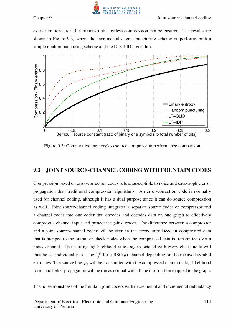
Chapter 9 Joint source -channel coding
every iteration after 10 iterations until lossless compression can be ensured. The results are
shown in Figure 9.3, where the incremental degree puncturing scheme outperforms both a
simple random puncturing scheme and the LT-CLID algorithm.
0 0.05 0.1 0.15 0.2 0.25 0.30
0.2
0.4
0.6
0.8
1
Bernoulli source constant (ratio of binary one symbols to total number of bits)
Com
pre
ssio
n / B
inary
entr
opy
Binary entropy
Random puncturing
LT−CLID
LT−IDP
Figure 9.3: Comparative memoryless source compression performance comparison.
9.3 JOINT SOURCE-CHANNEL CODING WITH FOUNTAIN CODES
Compression based on error-correction codes is less susceptible to noise and catastrophic error
propagation than traditional compression algorithms. An error-correction code is normally
used for channel coding, although it has a dual purpose since it can do source compression
as well. Joint source-channel coding integrates a separate source coder or compressor and
a channel coder into one coder that encodes and decodes data on one graph to effectively
compress a channel input and protect it against errors. The difference between a compressor
and a joint source-channel coder will be seen in the errors introduced in compressed data
that is mapped to the output or check nodes when the compressed data is transmitted over a
noisy channel. The starting log-likelihood ratios mc associated with every check node will
thus be set individually to ± log1−p
pfor a BSC(p) channel depending on the received symbol
estimates. The source bias ps will be transmitted with the compressed data in its log-likelihood
form, and belief propagation will be run as normal with all the information mapped to the graph.
The noise robustness of the fountain joint coders with decremental and incremental redundancy
Department of Electrical, Electronic and Computer Engineering 114University of Pretoria

Chapter 9 Joint source -channel coding
is shown [73] in this section. An input source with segments over the useful binary entropy
range was compressed by both the LT-IDP and LT-CLID compressors, before being transmitted
over a BSC and binary AWGN channel, where after the payload was decompressed. The
header was not corrupted, as it is not protected against noise. The decompressed output was
compared to the original input, and the bit error rate was measured for different channel noise
intensities. The results are shown for the BSC and the AWGN channel in Figures 9.4 and 9.5
respectively. It is shown that the CLID approach makes the payload more prone to errors after
decompression.
0 0.001 0.002 0.003 0.004 0.005 0.006 0.007 0.008 0.009 0.0110
−5
10−4
10−3
10−2
10−1
BSC p parameter [ratio]
Bit e
rro
r ra
te
LT−IDP (Decremental redundancy)
BSC p parameter
LT−CLID (Incremental redundancy)
LT−CLID Average
LT−IDP Average
Figure 9.4: A noise robustness comparison on the BSC.
Department of Electrical, Electronic and Computer Engineering 115University of Pretoria

Chapter 9 Joint source -channel coding
2 3 4 5 6 7 8 9 10 11
10−5
10−4
10−3
10−2
10−1
Eb/N
0
Bit e
rro
r ra
te
LT−IDP (Decremental redundancy)
LT−CLID (Incremental redundancy)
Bit error probability
LT−CLID Average
LT−IDP Average
Figure 9.5: Noise robustness comparison on a flat fading BI-AWGN channel.
Department of Electrical, Electronic and Computer Engineering 116University of Pretoria

CHAPTER 10
JOINT SOURCE -CHANNEL-NETWORK CODING
The main ‘arteries’ of wireless mesh networks are replete with two-way network coding
opportunities, where a centrally located relay can combine two packets intended for exchange
between two of its neighbouring nodes into one transmission. Additionally no opportunistic
listening or buffer content synchronisation is required, and compared to extended n-way
network coding throughput gain is maximised with two-way network coding. Deploying
this type of network coding can contribute significantly to network throughput without
requiring drastic changes in network operation or a large additional overhead. Most joint
channel-network coding techniques improve throughput and in [77] the linear property of the
channel code is used to reduce the computational complexity during network decoding. A joint
channel-network parity-check matrix is constructed in [78] where random network coding is
done. In [79] the relay forwards the XORed combination of the parity-check bits of the source
messages, and joint channel-network turbo decoding is done at the destination node. A joint
channel-network message passing decoding algorithm is given [80] for the destination node.
Motivated to develop a true joint source-channel-network code that compresses, adds
robustness against channel noise and network codes two input packets on a single bipartite
graph and iteratively decodes the intended packet on the same Tanner graph, an adaptation of the
fountain code of [81] is presented in this chapter. The proposed code (JSCNC) is shown through
extensive experimental analysis to outperform a separated joint source-channel and network
code (SSCNC), which is used in the traditional two-way network coding sense, in high source
entropy and high channel noise regions. The system model is firstly introduced, where the
Department of Electrical, Electronic and Computer Engineering 117University of Pretoria

Chapter 10 Joint source -channel -network coding
capacity of the joint source-channel-network coding scenario is given. The two-stage fountain
code implementation [81] of a joint source-channel code is revisited, where a computationally
efficient subroutine is contributed, as well as an analysis of how the intermediate error rate
translates to the system error rate. The joint source-channel-network code adaptation is also
discussed, and the separate and joint codes are experimentally compared. An outline of the
chapter is depicted in Figure 10.1.
Joint source-
channel-network
coding
System
model
Fountain code
compressor
Joint source-channel-
network coding
Numerical
analysis
Two-stage
method
Adapted two-stage
method
Figure 10.1: The chapter outline showing the topics that are covered.
10.1 SYSTEM MODEL
The bidirectional wireless relays that are considered, broadcast the sum of two packets received
from nodes A and B, so that A (respectively B) can discern the packet sent from B (resp. A) by
subtracting its own packet from the broadcast sum [8]. As seen in Figure 10.2, by transmitting
combined information the relay can exchange information between sources A and B in one
timeslot, instead of a separate timeslot for each of the two packets to be forwarded. No direct
communication link is assumed between nodes A and B.
The decode-recode-forward strategy employed by the relay must take into account the symbol
1-biased source entropies pA and pB of both packets A and B, the transmission channel noise ε
and the network coding required to combine both packets into one. For the network operating
in GF(2) and the relay-source channel being BSC(ε), the joint source-channel-network coding
Department of Electrical, Electronic and Computer Engineering 118University of Pretoria

Chapter 10 Joint source -channel -network coding
capacity C for the system is given in Equation (10.1).
C = 1 − H2(ε)
max (H2(pA),H2(pB))=
1 − H2(ε)
H2(p)(10.1)
SSCNC
A B
A BA
A BA
Joint source-channel code
Joint source-channel code
A
B
JSCNC
Joint source-channel-
network code
A
B
Figure 10.2: Two-way wireless network coding, and separate and joint source-channel and
network coding.
The binary entropy function is given by H2(·) and there is assumed to be no correlation between
the information in the two packets, or between the packets and the channel. In fact, the packets
and channel are independently generated as Bernoulli processes with the respective parameters.
The packet entropies are made equal in this study to simplify the analysis, in other words
pA = pB = p. Coding performance is gauged in terms of the mean of the bit error rates
experienced at nodes A and B after they have decoded their intended packets. Both packets A
and B consist of K bits, and the relay transmits N = υK/C coded bits to nodes A and B, where
υ > 1 is the coding overhead. After decoding packet B (resp. A) at node A (resp. B), the BER
(bit error rate) is measured as δA = K′B/K (resp. δB = K′
A/K) where K′
B(resp. K′
A) is the number
of errors in the recovered packet when compared to the correct one. The system BER δ is then
taken as the mean δ = (δA + δB)/2.
A joint source-channel code, with a XOR-based network code, and a joint
source-channel-network code (Figure 10.2) are evaluated in terms of the system BER.
The following section expounds on the implementation of the joint codes, which are based on
fountain codes.
Department of Electrical, Electronic and Computer Engineering 119University of Pretoria

Chapter 10 Joint source -channel -network coding
10.2 FOUNTAIN CODE COMPRESSOR
The two-stage fountain code compressor of [81] displayed in Figure 10.3, which utilises an
LT-code [48], is reviewed in this section. Fountain codes can produce an output stream of
varying length, which makes it more suitable for employment as a joint source-channel code
than LDPC or turbo codes.
Source input
Intermediate symbols
Output symbols
+-transform LT-code
Figure 10.3: Two-stage approach to joint source-channel coding with an LT-code.
In the two-stage compressor, a source input of K symbols (x1, . . . , xK) is mapped to K
intermediate symbols (y1, . . . , yK)T = Γ−1(x1, . . . , xK)T via a linearly invertible K × K matrix
Γ. This ensures that every input symbol participates in the resulting bipartite graph, unlike
the direct approach [73] where the probability of an unconnected input symbol is relatively
high. For the LT-code output degree distribution Ω(x) =∑K
d=1Ωd xd, the average input degree is
ζ = υΩ′(1)/C. Then with the input degree distribution Ψ(x) = (ζx/N + 1 − ζ/N)N , the fraction
of unrepresented input symbols with the direct approach is strongly dependent on the source
entropy and channel noise as shown by:
Ψ(0) =
(1 − ζ
N
)N
=
(1 − Ω
′(1)
K
)υK/C
(10.2)
The Hamming weights of the rows of Γ are sampled according to Ω(x), so that with the
additional N output symbols (xK+1, . . . , xK+N) the final Tanner graph can be interpreted
as a (K,Ω(x)) LT-code with input (y1, . . . , yK) and output (x1, . . . , xK+N). Through Belief
Propagation (BP) decoding (y1, . . . , yK) can be recovered, and consequently the original source
(x1, . . . , xK)T = Γ(y1, . . . , yK)T as well. The a-priori entropies for the intermediate symbols are
set to 0.5, for the input source symbols it is set to H2(p) and the reliabilities of the received
output symbols are set to be dependent on H2(ε).
A computationally efficient method of rendering a singular Γ invertible in GF(2), is to
Department of Electrical, Electronic and Computer Engineering 120University of Pretoria

Chapter 10 Joint source -channel -network coding
firstly calculate the row echelon form of [Γ I]. Here the last K − Rank(Γ) rows will point to
the constituent rows of Γ that contribute to the corresponding zero sum. Separately, for each
zero-sum row in the row echelon form, one of its constituent rows of Γ must be changed so that
the zero-sum row now sums to one of the K − Rank(Γ) absent variables in the echelon form.
The row echelon form must be re-evaluated until Rank(Γ) = K. In this manner the initial matrix
is reconditioned to achieve a fully sufficient row echelon form and thus be linearly invertible.
If an error rate of δy is experienced in the decoded intermediate symbols (y1, . . . , yK)
after BP decoding, then the resulting error rate δ of (x1, . . . , xK) can be approximated as in
(10.3). In practice this error rate translation has proven to be a surprisingly accurate upper
bound as shown in Figure 10.4.
δ(δy,Ω
)=
K∑
d=1
Ωd
⌊ d+12⌋∑
j=1
(d
2 j − 1
)δ2 j−1
y (1 − δy)d−2 j+1 (10.3)
0 0.05 0.1 0.15 0.2 0.25 0.3 0.35 0.4 0.45 0.50
0.1
0.2
0.3
0.4
0.5
Intermediate error rate [ δy ]
Syste
m e
rro
r ra
te [
δ ]
Observed upper bound
Theoretical upper bound
Figure 10.4: System error rate upper bound comparison.
The output symbols (xK+1, . . . , xK+N) are transmitted, in conjunction with the input source
entropy H2(p), and BP decoding is run on the reconstructed graph at the receiver side. When
used in the network coding scenario, the two sets of output symbols (xAK+1, . . . , xA
K+N) and
(xBK+1
, . . . , xBK+N
) generated by the joint source-channel coder for packets A and B are summed
together to (xAK+1 + xB
K+1, . . . , xAK+N + xB
K+N). Node A (resp. B) generates the same output
symbols (xAK+1
, . . . , xAK+N
) (resp. (xBK+1
, . . . , xBK+N
)) with packet A (resp. B) and subtracts it
from the received symbols A+B, the resulting packet is then decoded to recover the unknown
Department of Electrical, Electronic and Computer Engineering 121University of Pretoria

Chapter 10 Joint source -channel -network coding
packet (xBK+1
, . . . , xBK+N
) (resp. (xAK+1
, . . . , xAK+N
)). The implementation of an alternative joint
source-channel-network coder follows.
10.3 JOINT SOURCE-CHANNEL-NETWORK CODING
The network coding summation can be integrated into the joint code by inputting the
concatenation of packets A and B (Figure 10.5), which requires a new 2K × 2K matrix Γ to
map 2K input symbols (x1, . . . , xK , xK+1, . . . , x2K) to 2K intermediate symbols (y1, . . . , y2K).
The motivation of this approach is to evaluate the potential benefit that is gained by operating
on a Tanner graph of twice the size. The trade-off is higher complexity in BP decoding and
determining Γ−1 (in principle quadratic in K).
With the JSCNC (joint source-channel-network code) the same amount υK/C of output
symbols are generated as with the SSCNC (separate source-channel and network code), but
from twice the amount of intermediate symbols. In practice the output symbols are augmented
with the values of the intermediate symbols with the lowest reliability according to the
performed BP decoding (CLID [81]). The relay will perform this augmentation in a lossless
coding scenario with its estimate of the channel noise, and in the case of this enlarged code
two checks will be performed. The relay will append CLID symbols until it is reasonably
certain that both nodes A and B will be able to recover their respective packets. The number of
required CLID symbols can be estimated by δy.
Packet A
Intermediate symbols
Output symbols
+-transform LT-code
Packet B
Figure 10.5: Joint source-channel-network coding with a two-stage LT-code.
Node A (resp. B) will map the fully reliable symbols (x1, . . . , xK) (resp. (xK+1, . . . , x2K))
of packet A (resp. B) to the Tanner graph for BP decoding, and also the likelihood ratio
ln ((1 − pB)/pB) (resp. ln ((1 − pA)/pA)) of packet B (resp. A) to the appropriate input
nodes (xK+1, . . . , x2K) (resp. (x1, . . . , xK)) and the received channel output estimate LLRs
Department of Electrical, Electronic and Computer Engineering 122University of Pretoria

Chapter 10 Joint source -channel -network coding
(log-likelihood ratios) ln (ε/(1 − ε)) · (zA1, . . . , zA
N) (resp. ln (ε/(1 − ε)) · (zB
1, . . . , zB
N)) to the
output nodes (x2K+1, . . . , x2K+N). Here the relay hard output bits received by node A and B
are given by (zA1, . . . , zA
N) and (zB
1, . . . , zB
N) respectively. The CLID symbols can be used during
the BP decoding to ensure lossless decoding with high probability. The experimental results are
analysed in the next section.
10.4 NUMERICAL ANALYSIS
The system error rates δ of the separate and joint codes (SSCNC and JSCNC) for all
combinations of source entropies p and channel noise ε are compared in this section.
Independent Mersenne twisters were used to produce 100 different code, source and channel
realisations for every (p, ε) pair coded by both codes, so that high quality error rate estimations
could be obtained through averaging. The receivers were assumed to have perfect knowledge
of the channel noise level ε.
A good joint source-channel code has to perform well simultaneously on the BEC (binary
erasure channel) and BSC channels, so that it can compress and protect data sufficiently.
Therefore an LT-code output degree distribution of Ω(x) = 0.008x + 0.494x2 + 0.166x3 +
0.073x4 + 0.083x5 + 0.056x8 + 0.037x9 + 0.056x19 + 0.025x65 + 0.003x66 is chosen, which was
shown to perform satisfactory on the aforementioned channels (see [81]).
The source length was set as K = 5000 and a coding overhead of υ = 1.2 was chosen
throughout for every (p, ε) and both joint codes, which means that the codes are operating at
83.3% of system capacity. BP decoding was limited to 100 iterations and a maximum LLR
of 25 was adopted. CLID was not performed for any of the joint codes, so that the code
performance could be directly determined.
The mean bit error rates of the decoded packets are compared for the two joint codes
for different source entropies and channel noises in Figures 10.6 and 10.7. In the high
source and channel entropy regions, the joint code (JSCNC) outperforms the separated joint
source-channel and network code (SSCNC), at the expense of notably poor performance for
ε ≤ 0.1 and p ≤ 0.05. The separated coding performs well under the entire range of (p, ε), but
is outperformed in the high entropy and noise regions by the joint code.
The proposed joint source-channel-network code effectively doubles the code block length
Department of Electrical, Electronic and Computer Engineering 123University of Pretoria

Chapter 10 Joint source -channel -network coding
0.1 0.2 0.30
0.1
0.2
0.3
0.4
Source bias [ p ]
Bit e
rro
r ra
te [
ra
tio
]
0.1 0.2 0.30
0.02
0.04
0.06
0.08
0.1
Source bias [ p ]
Bit e
rro
r ra
te [
ra
tio
]
0.1 0.2 0.30
0.01
0.02
0.03
0.04
0.05
Source bias [ p ]
Bit e
rro
r ra
te [
ra
tio
]
0.1 0.2 0.30
0.01
0.02
0.03
0.04
0.05
Source bias [ p ]
Bit e
rro
r ra
te [
ra
tio
]
SSCNCJSCNC
SSCNCJSCNC
SSCNCJSCNC
SSCNCJSCNC
ε=0.1 ε=0.2
ε=0.3 ε=0.4
Figure 10.6: System error rates δ vs. source entropy p for different channel noises ε.
0.1 0.2 0.30
0.1
0.2
0.3
0.4
BSC error parameter [ ε ]
Bit e
rro
r ra
te [
ra
tio
]
0.1 0.2 0.30
0.01
0.02
0.03
0.04
BSC error parameter [ ε ]
Bit e
rro
r ra
te [
ra
tio
]
0.1 0.2 0.30
0.005
0.01
0.015
BSC error parameter [ ε ]
Bit e
rro
r ra
te [
ra
tio
]
0.1 0.2 0.30
0.005
0.01
0.015
BSC error parameter [ ε ]
Bit e
rro
r ra
te [
ra
tio
]
SSCNCJSCNC
SSCNCJSCNC
SSCNCJSCNC
SSCNCJSCNC
p=0.05 p=0.15
p=0.25 p=0.35
Figure 10.7: System error rates δ vs. channel noise ε for different source entropies p.
Department of Electrical, Electronic and Computer Engineering 124University of Pretoria

Chapter 10 Joint source -channel -network coding
which benefits performance for high source entropies and channel noise realisations, when
compared to the separated code. The astute reader would have recognised the opportunity
to artificially increase the Tanner graph length with predetermined data at both the relay and
source nodes, to harness a bigger code for improving performance in the high entropy-noise
regions, similar to what is achieved by the joint source-channel-network code presented in this
chapter. Furthermore, the joint source-channel code itself can be artificially lengthened for
high entropy-noise performance, although at the expense of an increased error rate in the low
entropy-noise region.
Department of Electrical, Electronic and Computer Engineering 125University of Pretoria

CHAPTER 11
CONCLUSIONS ANDFUTURE RESEARCH
11.1 CONCLUSION
A temporal reuse-aware cross-layer optimisation framework for multihop wireless mesh
networks was designed in this dissertation, as well as a truly joint three-way
source-channel-network code. The research questions that guided the investigations are
reviewed and the contributions and conclusions are discussed for each of the two featured topics.
11.1.1 Cross-layer optimisation of wireless networks with temporal reuse
The first research question that has been addressed in this study is as follows: What generic
transmission scheduling algorithm can produce predefined link-assigned schedules that
maximise schedule capacity with proportionally fair end-to-end flow rates for quasi-stationary
multihop mesh networks with single-path minimum hop routing, rate and power adaptivity,
both spatial and temporal reuse and network coding?
The following contributions were made in answering this question:
1. The hybrid node-link assignment strategy of [1] was re-evaluated in terms of a new
concept that is defined here, namely temporal reuse, which is recognised as the
time-domain analogue of spatial reuse.
2. A specific characterisation of the schedules that could induce packet depletion was given,
and it was then shown that optimal schedules can potentially benefit from higher usage
Department of Electrical, Electronic and Computer Engineering 126University of Pretoria

Chapter 11 Conclusions and future research
efficiency afforded by temporal reuse.
3. A new achievable rate region was formulated that provides better estimates of the
increased link capacities due to temporal reuse. The rate region was derived to be generic,
meaning that only information on the network topology and data flows are needed to
calculate its capacity without having to simulate the network in question.
4. A cross-layer optimisation scheduling algorithm was given that uses the newly proposed
rate region and solves the scheduling subproblem with temporal reuse in mind.
Firstly, it was experimentally shown that by optimising schedules with temporal reuse in
the temporal reuse-aware rate region the schedule capacity is increased when compared to
optimisation in the non-aware rate region of [32]. In addition, flow rate fairness is also
improved with the proposed scheduler and the benefit derived from network coding is also
greater. For schedules with rate and power adaptivity it was shown that the proposed scheduler
achieves better power efficiency.
The relationship between spatial and temporal reuse was analysed and the temporal reuse-aware
scheduler managed a more effective balance for the different rate and power adaptivities. The
trade-off between schedule capacity and fairness was affirmed and it was shown that the
proposed class of optimised link-assigned schedules outperforms node-assigned schedules in
that respect.
11.1.2 Joint source-channel-network coding
The second research question was: Can a truly joint three-way source-channel-network coding
algorithm, based on fountain codes outperform a separated joint source-channel and network
code (joint source-channel code and separate network code) in a high noise and high entropy
coding region?
A number of contributions were made in answering this research question, some of which are
as follows:
1. A structural comparison was made between sparse graph LDPC codes and fountain codes,
where the relationship between the degree distributions of the codes were made evident.
Department of Electrical, Electronic and Computer Engineering 127University of Pretoria

Chapter 11 Conclusions and future research
2. It was shown how density evolution could be used to optimise the degree distributions
of fountain codes, for its uses in channel coding, joint source-channel coding and joint
source-channel-network coding.
3. An efficient algorithm for rendering singular matrices in GF(2) invertible was explained
to facilitate the design of a two-stage joint coding approach with fountain codes.
4. An error-translation analysis was done for the two-stage joint source-channel coding
algorithm based on fountain codes.
5. A scheme was explained for a truly joint source-channel-network code based on the
two-stage joint source-channel coding approach with fountain codes.
The novel adaptation of the two-stage fountain code compressor [81] for use in a
joint source-channel-network code effectively doubles the code block length, and it was
experimentally shown that this approach outperforms a separated source-channel and network
code in the high noise and high entropy coding regions.
11.2 FUTURE RESEARCH
The possible avenues of extended or additional research in the topics addressed in this study
are listed and discussed in this section. The future research that deserves attention is handled
separately for cross-layer optimisation of wireless mesh networks with temporal reuse and joint
source-channel-network coding.
11.2.1 Cross-layer optimisation of wireless networks with temporal reuse
Possible extensions of the network methods to which the study is limited include multipath
routing, cooperative coding and more complex n-way (n > 2) network coding.
11.2.1.1 Multipath routing
Changing the routing from single-path minimum hop routing to multipath routing has the
potential to reduce congestion in a multihop mesh network, amongst other benefits. Usually
the path decisions depend on the current network state and traffic for multipath routing, which
complicates the scheduling optimisation. Methods may be studied to reliably calculate network
capacity regions for networks with multipath routing and temporal reuse.
Department of Electrical, Electronic and Computer Engineering 128University of Pretoria

Chapter 11 Conclusions and future research
11.2.1.2 Cooperative coding
Network coding presents a very basic form of cooperative coding, where neighbouring nodes
work together to accomplish a non-standard coding effect. More complicated forms of
cooperative coding exist and these may be incorporated into a simulation environment to test
the temporal reuse-aware optimised scheduling. Possible amendments can improve the schedule
optimisation for networks with cooperative coding.
11.2.1.3 Multi-way network coding
This study focuses on the most efficient case of network coding, namely two-way network
coding, in the absence of opportunistic listening. The optimisation framework contributed in
this dissertation could be re-evaluated to give improved results in the presence of opportunistic
listening and more complex n-way (n > 2) network coding.
11.2.2 Joint source-channel-network coding
Some of the areas of improvement for the joint coding investigated in this dissertation include
degree distribution optimisation, implementation in wireless mesh networks, low entropy-noise
region performance increases and the study of other channel models. Extensions of the joint
code for multi-way network coding is also a possible research outlet.
11.2.2.1 Degree distribution optimisation
While the density evolution methods for fountain codes were discussed in this study, they were
not used to optimise the output degree distribution for the joint source-channel-network codes.
The degree distribution optimisation tools given in this dissertation can be used to optimise the
joint source-channel-network codes proposed in this work.
11.2.2.2 Implementation in wireless networks
The various ways in which a joint code can be integrated in wireless mesh network operation
could be investigated, in order to synthesize the complete implementation details. This
dissertation presented one of many approaches to enable network coding support for a network,
but there is scope for further detailed investigation of the actual implementation of joint coding.
Department of Electrical, Electronic and Computer Engineering 129University of Pretoria

Chapter 11 Conclusions and future research
11.2.2.3 Low entropy-noise region performance
Future research could investigate modifications to the proposed joint source-channel-network
code to improve its low entropy-noise performance to equal that of the separated joint
source-channel and network code. This could produce a joint code that is fit for any
source-channel environment.
11.2.2.4 Channel models
The joint codes in this study has been designed for binary symmetric noise channels, but the
codes could be redesigned for other channel models and the performance can be measured to
determine if there are some channels that are more appropriate for these codes.
Department of Electrical, Electronic and Computer Engineering 130University of Pretoria

REFERENCES
[1] J. Gronkvist, “Novel assignment strategies for spatial reuse TDMA in wireless ad hoc
networks,” Wireless Networks, vol. 12, no. 2, pp. 255–265, March 2006.
[2] J. Jubin and J. Tornow, “The DARPA packet radio network protocols,” in Proc. of the
IEEE 75 (1), January 1987.
[3] M. Matsumoto and T. Nishimura, “Mersenne twister: a 623-dimensionally equidistributed
uniform pseudo-random number generator,” ACM Trans. on Modeling and Computer
Simulation, vol. 8, no. 1, pp. 3–30, 1998.
[4] P. Gupta and P. Kumar, “The capacity of wireless networks,” IEEE Trans. Inf. Theory,
vol. 46, pp. 388–404, March 2000.
[5] E. W. Dijkstra, “A note on two problems in connexion with graphs,” Numerische
Mathematik, vol. 1, pp. 269–271, 1959.
[6] R. Bellman, Dynamic Programming, isbn 0486428095 ed. Princeton University Press,
Princeton, NJ (Republished 2003: Dover), 1957.
[7] R. Ahlswede, N. Cai, S.-Y. Li, and R. Yeung, “Network information flow,” IEEE Trans.
Inf. Theory, vol. 46, no. 4, pp. 1204 –1216, Jul. 2000.
[8] S. Katti, H. Rahul, W. Hu, D. Katabi, M. Medard, and J. Crowcroft, “XORs in the air:
Practical wireless network coding,” IEEE/ACM Trans. Netw., vol. 16, no. 2, pp. 497–510,
2008.
[9] C. Fragouli, J. L. Boudec, and J. Widmer, “Network coding: An instant primer,” ACM
SIGCOMM Comput. Commun. Rev., vol. 36, no. 1, pp. 63–68, January 2006.
[10] K. Menger, “Zur allgemeinen Kurventheorie,” Fund. Math., vol. 10, pp. 95–115, 1927.
Department of Electrical, Electronic and Computer Engineering 131University of Pretoria

References
[11] S. Li, R. Yeung, and N. Cai, “Linear network coding,” IEEE Trans. Inf. Theory, vol. 49,
no. 2, pp. 371–381, February 2003.
[12] R. Koetter and M. Medard, “An algebraic approach to network coding,” IEEE/ACM Trans.
Netw., vol. 11, no. 5, pp. 782–795, October 2003.
[13] T. Ho, M. Medard, R. Koetter, D. Karger, M. Effros, J. Shi, and B. Leong, “A random
linear network coding approach to multicast,” IEEE Trans. Inf. Theory, vol. 52, no. 10, pp.
4413–4430, October 2006.
[14] P. Chou, Y. Wu, and K. Jain, “Practical network coding,” in Proc. 41st Annu. Allerton
Conf. Communication, Control and Computing, October 2003, Monticello, IL.
[15] S. Biswas and R. Morris, “Opportunistic routing in multi-hop wireless networks,” in Proc.
ACM SIGCOMM, August 2005, pp. 133–144.
[16] C. Gkantsidis and P. Rodriguez, “Network coding for large scale content distribution,”
in INFOCOM 2005. 24th Annu. Joint Conf. of the IEEE Computer and Communications
Societies., vol. 4, March 2005, pp. 2235 – 2245 vol. 4.
[17] M. Wang and B. Li, “R2: Random push with random network coding in live peer-to-peer
streaming,” IEEE J. Sel. Areas in Commun., vol. 25, no. 9, pp. 1655 –1666, December
2007.
[18] S. Zhang, S.-C. Liew, and P. P. Lam, “Physical-layer network coding,” in ACM Mobicom
06, 2006.
[19] P. Karn, “MACA: A new channel access method for packet radio,” in Proc. of the
ARRL/CRRL Amateur Radio 9th Computer Netw. Conf., 1990, pp. 134–140.
[20] V. Bharghavan, A. Demers, S. Shenker, and L. Zhang, “MACAW: Media access protocol
for wireless LANs,” in Proc. of the ACM SIGCOMM Conf., 1994.
[21] J. Garcia-Luna-Aceves and C. L. Fullmer, “Floor acquisition multiple access (FAMA) in
single-channel wireless networks,” in Mobile Networks and Applications (Springer), 1998,
pp. 262–273.
[22] F. Talucci, M. Gerla, and L. Fratta, “MACA-BI (MACA by invitation) - A receiver oriented
access protocol for wireless multihop networks,” in Proc. IEEE PIMRC, 1997.
Department of Electrical, Electronic and Computer Engineering 132University of Pretoria

References
[23] J. Garcia-Luna-Aceves and A. Tzamaloukas, “Reversing the collision-avoidance
handshake in wireless networks,” in Proc. of ACM/IEEE Mobicom, 1999.
[24] I. Cidon and M. Sidi, “Distributed assignment algorithms for multihop packet radio
network,” IEEE Trans. Comput., vol. 38, no. 4, pp. 456–460, 1990.
[25] I. Chlamtac and S. Kutten, “A spatial reuse tdma/fdma for mobile multi-hop radio
networks,” in IEEE InfoCom ’85, vol. 1, 1985, pp. 389–394.
[26] B. Hajek and G. Sasaki, “Link scheduling in polynomial time,” IEEE Trans. Inf. Theory,
vol. 35, no. 5, pp. 910–917, 1988.
[27] I. Chlamtac and A. Lerner, “A link allocation protocol for mobile multi-hop radio
networks,” in IEEE GlobeCom ’85, vol. 1, 1985, pp. 238–242.
[28] L. Pond and V. Li, “A distributed time-slot assignment protocol for multi-hop broadcast
packet radio networks,” in IEEE MilCom, vol. 1, October 1989, pp. 70–74.
[29] K. Papadaki and V. Friderikos, “Approximate dynamic programming for link scheduling
in wireless mesh networks,” Computers&Operations Research, vol. 35, no. 12, December
2007.
[30] J. Gronkvist, “Traffic controlled spatial reuse TDMA in multi-hop radio networks,” in
PIMRC, 1998, pp. 1203–1207.
[31] F. Luus and B. Maharaj, “Cross-layer optimization of wireless networks with extended
transmission rights,” in GLOBECOM 2010, 2010 IEEE Global Telecommun. Conf.,
December 2010, pp. 1 –5.
[32] M. Johansson and L. Xiao, “Cross-layer optimization of wireless networks using nonlinear
column generation,” IEEE Trans. on Wireless Commun., vol. 5, no. 2, Feb. 2006.
[33] S. Toumpis and A. Goldsmith, “Capacity regions for wireless ad hoc wireless networks,”
IEEE Trans. on Wireless Commun., vol. 2, no. 4, pp. 736–748, 2003.
[34] C. Caratheodory, “Uber den variabilitatsbereich der fourierschen konstanten von positiven
harmonischen funktionen,” Rend. Circ. Mat. Palermo, vol. 32, pp. 193–217, 1911.
[35] B. Radunovic and J.-Y. Boudec, “Rate performance objectives of multihop wireless
networks,” IEEE Trans. on Mobile Computing, vol. 3, no. 4, pp. 334–349, Oct.-Dec. 2004.
Department of Electrical, Electronic and Computer Engineering 133University of Pretoria

References
[36] ——, “Joint scheduling, power control and routing in symmetric one-dimensional,
multi-hop wireless networks,” in WiOpt’03, Sophia Antipolis, France, 2003, pp. 31–42.
[37] F. Kelly, A. Malulloo, and D. Tan, “Rate control in communications networks: shadow
prices, proportional fairness and stability,” J. Operational Research Society, vol. 49, pp.
237–252, 1998.
[38] P. Varbrand, P. Bjorklund, and D. Yuan, “Resource optimization of spatial TDMA in
ad hoc radio networks: A column generation approach,” in IEEE InfoCom 2003, San
Francisco, March 2003.
[39] P. Soldati, B. Johansson, and M. Johansson, “Proportionally fair allocation of end-to-end
bandwidth in STDMA wireless networks,” in ACM MobiHoc ’06, Florence, Italy, May
2006.
[40] S. Low and D. Lapsley, “Optimization flow control - I:Basic algorithm and convergence,”
IEEE/ACM Trans. Netw., vol. 7, no. 6, pp. 861–874, December 1999.
[41] A. Wachter and L. Biegler, “On the implementation of a primal-dual interior point
filter line search algorithm for large-scale nonlinear programming,” Mathematical
Programming, vol. 106, no. 1, pp. 25–57, 2006.
[42] C. Shannon, “A mathematical theory of communication,” Bell Systems Technical Journal,
vol. 27, pp. 623–656, 1948.
[43] P. Elias, “Coding for two noisy channels,” in Inform. Theory, Third London Symposium,
1955, pp. 61–76.
[44] E. Berlekamp, R. McEliece, and H. van Tilborg, “On the inherent intractability of certain
coding problems,” IEEE Trans. Inf. Theory, vol. 24, pp. 384–386, 1978.
[45] P. Elias, “Coding for noisy channels,” in IRE Conv. Record, 1955, pp. 37–47.
[46] M. J. E. Golay, “Notes on digital coding,” in Proc. IEEE, vol. 36, 1949, p. 657.
[47] R. G. Gallager, “Low density parity-check codes,” Ph.D. dissertation, MIT Press,
Cambridge, MA, 1963.
[48] M. Luby, “LT-codes,” in Proc. 43rd Annu. IEEE Symp. Foundations of Comp. Science,
Nov. 2002, pp. 271–280.
Department of Electrical, Electronic and Computer Engineering 134University of Pretoria

References
[49] D. MacKay, Information Theory, Inference, and Learning Algorithms. Cambridge
University Press, 2003.
[50] M. G. Luby, M. Mitzenmacher, M. A. Shokrollahi, and D. A. Spielman, “Efficient erasure
correcting codes,” IEEE Trans. Inf. Theory, vol. 47, pp. 569–584, February 2001.
[51] J. Pearl, Probabilistic Reasoning in Intelligent Systems: Networks of Plausible Inference.
Morgan Kaufmann Publishers, Inc., 1988.
[52] M. Luby, M. Mitzenmacher, A. Shokrollahi, and D. Spielman, “Analysis of low density
codes and improved designs using irregular graphs,” IEEE Trans. Inf. Theory, vol. 47, pp.
585–598, 2001.
[53] T. Richardson and R. Urbanke, “The capacity of low-density parity-check codes under
message-passing decoding,” IEEE Trans. Inf. Theory, vol. 47, no. 2, pp. 599–618, Feb
2001.
[54] T. Richardson, A. Shokrollahi, and R. Urbanke, “Design of capacity-approaching irregular
low- density parity-check codes,” IEEE Trans. Inf. Theory, vol. 47, pp. 619–637, 2001.
[55] T. Richardson and R. Urbanke, Modern Coding Theory. Cambridge University Press,
2008.
[56] O. Etesami and A. Shokrollahi, “Raptor codes on binary memoryless symmetric
channels,” IEEE Trans. Inf. Theory, vol. 52, no. 5, pp. 2033–2051, May 2006.
[57] O. Etesami, M. Molkaraie, and A. Shokrollahi, “Raptor codes on symmetric channels,” in
IEEE Int. Symp. Inform. Theory, June 2004, p. 38.
[58] R. Palanki and J. Yedidia, “Rateless codes on noiseless channels,” in IEEE Int. Symp. on
Inform. Theory, June 2004, p. 37.
[59] P. Mitran and J. Bajcsy, “Turbo source coding: A noise-robust approach to data
compression,” in Proc. DCC’02, April 2002, pp. 465–465.
[60] E. Weiss, “Compression and coding,” IRE Trans. on Inform. Theory, pp. 256–257, April
1962.
[61] P. E. Allard and A. W. Bridgewater, “A source encoding technique using algebraic codes,”
in 1972 Canadian Computer Conf., June 1972, pp. 201–213.
Department of Electrical, Electronic and Computer Engineering 135University of Pretoria

References
[62] K. C. Fung, S. Tavares, and J. M. Stein, “A comparison of data compression schemes using
block codes,” in IEEE Int. Electrical and Electronics Conf., October 1973, pp. 60–61.
[63] T. Ancheta, “Syndrome source coding and its universal generalization,” IEEE Trans. Inf.
Theory, vol. 22, no. 4, pp. 432–436, July 1976.
[64] H. Ohnsorge, “Data compression system for the transmission of digitalized signals,” in
IEEE Int. Conf. on Commun., vol. 2, June 1973, pp. 485–488.
[65] J. Garcia-Frias and Y. Zhao, “Compression of binary memoryless sources using punctured
turbo codes,” IEEE Commun. Lett., vol. 6, pp. 394–396, September 2002.
[66] G. Caire, S. Shamai, and S. Verdu, “A new data compression algorithm for sources with
memory based on error correcting codes,” in 2003 IEEE Workshop on Inform. Theory,
April 2003, pp. 291–295.
[67] ——, “Lossless data compression with error correction codes,” in 2003 IEEE Int. Symp.
on Inform. Theory, July 2003, p. 22.
[68] G. Caire, S. Shamai, and Verdu, “Universal data compression with LDPC codes,” in Proc.
of Third Int. Symp. On Turbo Codes and Related Topics, Sept. 2003, pp. 55–58, Brest,
France.
[69] G. Caire, S. Shamai, A. Shokrollahi, and S.Verdu, “Fountain codes for lossless data
compression,” DIMACS Series in Discrete Mathematics and Theoretical Computer
Science, 2005.
[70] G. Caire, S. Shamai, and S. Verdu, “Noiseless data compression with low density
parity check codes,” DIMACS Series in Discrete Mathematics and Theoretical Computer
Science, vol. 66, pp. 263–284, 2004.
[71] B. McMillan, “The basic theorems of information theory,” Ann. Math. Statist., vol. 24, pp.
196–219, June 1953.
[72] I. Csiszar and J. Korner, Information theory: Coding theorems for discrete memoryless
systems. New York: Academic, 1981.
Department of Electrical, Electronic and Computer Engineering 136University of Pretoria

References
[73] B. Maharaj and F. Luus, “Decremental redundancy compression with fountain codes,”
in Netw. and Commun., 2008. WIMOB ’08. IEEE Int. Conf. on Wireless and Mobile
Computing,, 2008, pp. 328–332.
[74] F. Luus, A. McDonald, and B. Maharaj, “Universal decremental redundancy compression
with fountain codes,” SAIEE Africa Research Journal, vol. 101, no. 2, pp. 68–77, June
2010.
[75] M. Burrows and D. J. Wheeler, “A block-sorting lossless data compression algorithm,” in
Tech. Rep. SRC 124, May 1994.
[76] N. Dutsch, “Code optimisation for lossless compression of binary memoryless sources
based on fec codes,” Euro. Trans. Telecomms, vol. 17, pp. 219–229, 2006.
[77] S. Zhang, Y. Zhu, S.-C. Liew, and K. Letaief, “Joint design of network coding and channel
decoding for wireless networks,” in Proc. of IEEE WCNC 2007, March 2007, pp. 779–784,
Hong Kong.
[78] D. Bing and Z. Jun, “Design and optimisation of joint network-channel LDPC code
for wireless cooperative communications,” in Proc. 11th IEEE Singapore Int. Conf. on
Commun. Systems (ICCS 2008), 2008, pp. 1625–1629.
[79] S. Tang, J. Cheng, C. Sun, R. Suzuki, and S. Obana, “Turbo network coding for efficient
and reliable relay,” in Proc. ICCS 2008, 2008, pp. 1603–1608.
[80] X. Xu, M. Flanagan, and N. Goertz, “A shared-relay cooperative diversity scheme based
on joint channel and network coding in the multiple access channel,” in Proc. 5th Int.
Symp. on Turbo Codes and Related Topics, 2008, pp. 243–248.
[81] G. Caire, S. Shamai, A. Shokrollahi, and S. Verdu, “Universal variable-length data
compression of binary sources using fountain codes,” in Proc. of IEEE Inform. Theory
Workshop, 2004, pp. 123–128.
Department of Electrical, Electronic and Computer Engineering 137University of Pretoria