Joint inversion of AVA data for elastic parameters by

ARTICLE IN PRESS

0098-3004/$ - se

doi:10.1016/j.ca

�Tel.: +90 2

E-mail addr

Computers & Geosciences 33 (2007) 367–382

www.elsevier.com/locate/cageo

Joint inversion of AVA data for elastic parametersby bootstrapping

Hulya Kurt�

Istanbul Technical University, Department of Geophysics, 34390-Maslak, Istanbul, Turkey

Received 27 February 2006; received in revised form 24 August 2006; accepted 27 August 2006

Abstract

A joint inversion method is developed to estimate the elastic constants of two elastic, homogeneous, isotropic media

separated by a flat horizontal boundary. The method jointly uses P and S-converted wave reflection amplitude-versus-

angle (AVA) data and seeks the Poisson’s ratios of each layer, ratios of the densities and bulk modulus of the layers. The

generalized linear inversion (GLI) method is used as a mathematical tool and the Zoeppritz equations defining the seismic

energy partitioning at a boundary are used as the physical model.

The P and S-converted wave velocity terms in the Zoeppritz equations were replaced by the bulk modulus ðk1; k2Þ,

Poisson’s ratios ðs1; s2Þ, and densities ðr1; r2Þ of each layer. After expressing the equations in these six elastic constants,

reflection coefficients of P and S-converted waves ðRpp;RpsÞ are obtained as functions of ratios of bulk modulus and

densities of the lower layer to those of the upper layer (k2=k1 and r2=r1) and Poisson’s ratios of the upper and lower layers

(s1 and s2Þ. Using the ratios of bulk modulus and densities, the number of unknown parameters is reduced from 6 to 4 and

this improves the success of inversion. The other contribution is that the calculation of Rpp and Rps and their derivatives

with respect to elastic constants and their ratios in the inversion are calculated analytically and coded in the Fortran

programming language. In this way, the approach has an important advantage among the other AVA inversion methods,

which are mostly based on numerical solutions or approximations to the Zoeppritz equations. A bootstrapping method of

statistical analysis is combined with the GLI method to find the most likely elastic parameters and their confidence limits

for repeated inversions for a large number of times by rearranging the noise distribution of the AVA data.

r 2006 Elsevier Ltd. All rights reserved.

Keywords: AVA; Joint inversion; Elastic parameters; Bootstrapping; Zoeppritz equations

1. Introduction

Variation of seismic reflection and transmissioncoefficients with angle of incidence has been widelyinvestigated to extract information about the lithol-ogy and subsurface elastic parameters (Ostrander,1984; Backus, 1987; Rutherford and Williams,

e front matter r 2006 Elsevier Ltd. All rights reserved

geo.2006.08.012

12 2856255; fax: +90 212 2856201.

ess: [email protected].

1989). Seismic amplitude-versus-offset (AVO) andamplitude-versus-angle (AVA) data contain infor-mation about the elastic parameters of the subsur-face. The Zoeppritz equations describe the reflectionand transmission coefficients for plane waves as afunction of incidence angle and six independentseismic parameters (P and S wave velocities, anddensity of the upper and lower media) (Berkhout,1987). The equations were developed by Zoeppritz(1919), described in matrix form by Aki and

.

www.elsevier.com/locate/cageo

dx.doi.org/10.1016/j.cageo.2006.08.012

mailto:[email protected]

ARTICLE IN PRESSH. Kurt / Computers & Geosciences 33 (2007) 367–382368

Richards (2002) and their various analytic approx-imate forms are published in the literature (Bortfeld,1961; Shuey, 1985). Lavaud et al. (1999), reparame-terize the full equation in terms of a background andthree contrasting parameters and use singular valuedecomposition analysis to study information contentof P and P-converted S-wave AVO data.

Inversion of seismic AVO/AVA data for physicalproperties that enables direct lithological interpreta-tion has been applied to the estimation of elasticparameters especially in reservoir rocks. AVO/AVAinversion can be performed either in the x–t domain(Dahl and Ursin, 1992; Mahob et al., 1999) or in thet–p domain (Carazzone and Srnka, 1993; Bulandet al., 1996). Linear or nonlinear approaches ofAVO/AVA inversion methods can be carried out ineither 2 dimensions (2D) or 3 dimensions (3D). Thelinearized inversion of 2D AVO data in x–t domainis performed to find P-wave velocities, S-wavevelocities and density ratios of two-layered hor-izontal models (Demirbag et al., 1993). In theirstudy, the most likely solutions and confidencelimits are estimated by a bootstrapping method.A Bayesian approach is also used in AVO inversionstudies with probabilistic estimates of the unknownparameters from uncertain data and apriori infor-mation. Nonlinear inversion of AVO data by theBayesian formulation provides the estimates ofuncertainties of the viscoelastic physical parametersat an interface (Riedel et al., 2003). A 3D linearizedAVO inversion method in a Bayesian frameworkwith spatially coupled model parameters is devel-oped to obtain posterior distributions for P-wave,S-wave velocity and density (Buland et al., 2003).

Joint analysis and inversion of reflected P-waves(PP) and S-converted waves (PS) in AVO/AVAdata should provide better estimates of elasticparameters when compared with the standardP-wave approach alone. A practical method forthe joint inversion of PP and PS reflectioncoefficients is described and applied to field datain the study of Margrave et al. (2001). The resultsfrom joint inversion are better because the ambi-guities in the PP-only data are reduced. Variousdata sets are also used for inversion of AVO, e.g., ajoint AVO inversion procedure of seismic data andwell-log data are used to estimate P-wave, S-wavevelocity and density as well as seismic wavelet andseismic-noise level (Buland and More, 2003). Bothtravel times and amplitudes are jointly used in theinversion to find elastic parameters at the reflectors(Wang, 1999; Buland and Landrø, 2001).

Estimation of rock properties (elastic moduli)directly from AVO data may give more physicalinsights than classical parameters of P and S

velocities, and density. For example, Young’s mod-ulus is an appropriate modulus for describing theeffects of pressure upon rock properties. Pigott et al.(1989) have suggested that this elastic constant can bedynamically determined from the inversion of AVOdata. Stewart et al. (1995) show that Lame parameters(l-compressibility and m-shear) of the medium betterdifferentiate rock properties. Similarly, a joint inver-sion AVA study by Goodway et al. (1997) shows thatl, m and l=m parameters are more sensitive to changesin rock properties than P and S wave velocities (Vp

and V sÞ and Vp=V s. Estimation of rock propertiessuch as lithology, porosity, and pore fluid content areneeded for quantitative extraction of rock propertiesby AVO analysis. The bulk modulus of the rocks (k,rock incompressibility), which defines the ratio ofvolumetric stress to volumetric strain, is stronglydependent on the pore fluid of rocks (Domenico,1977). Poisson’s ratio has a strong influence onchanges in reflection coefficient as a function ofincidence angle. Theory and laboratory measurementsindicate that high-porosity gas sands tend to exhibitabnormally low Poisson’s ratios (Ostrander, 1984).Density contrasts give important information aboutthe lithology or the fluid saturation of the reservoir.

In this paper, a technique is developed to performa joint AVA inversion of P and S-converted wavesfrom prestack seismic reflection data. The methodestimates the ratios of bulk moduli ðrkÞ and densityðrrÞ of the lower layer to those of the upper layer(k2=k1 and r2=r1) and Poisson’s ratios of the upperand lower layers (s1 and s2Þ of two elastic mediumseparated by a horizontal boundary. Because bulkmoduli and density contrasts and Poisson’s ratio aresensitive to lithology, porosity and pore fluidcontents of rocks that affect seismic amplitudes,these elastic constants are chosen as model para-meters along with densities. The number of un-known parameters in the inversion proceduredecreases from 6 to 4 by taking the contrasts ofthe bulk moduli and densities rather than individualvalues of k1, k2, r1, r2. The full form of the P and S

wave reflection coefficients are expressed analyti-cally in linear equation systems from the Zoeppritzequations. Moreover, the derivatives of Rpp and Rps

with respect to the unknown parameters of theJacobian matrix are formed analytically providingan increase in the sensitivity and reliability of theinversion. Amplitudes are normalized to the values

ARTICLE IN PRESSH. Kurt / Computers & Geosciences 33 (2007) 367–382 369

of the first angle, i.e., 1� (Rppð1Þ and Rpsð1Þ) insteadof 0� as in traditional AVO/AVA studies. This isdone in order to avoid uncertainty in the analyticalcomputation of the Jacobian derivatives at zerodegree angle of incidence of reflections. The expres-sions of Rpp and Rps are nonlinear functions of thesearched parameters rk, rr, s1 and s2. Residualfunction maps (RFM) (Demirbag et al., 1993) areused to investigate the degree of nonlinearity in thegeneralized inversion method. Statistically signifi-cant mean values and standard deviations to beused as inputs in inverse simulations were generatedfrom a database using a bootstrapping method(Efron and Gong, 1983). Two reservoir models areused to test the inversion method and results areenhanced by the bootstrapping and compared forthe presence of random noise.

1.1. The Zoeppritz equations as functions of elastic

parameters

The physical model of this study is the Zoeppritzequations, which describes the energy partitioning

sin y1 cosfr � sin yt cosft

� cos y1 sinfr � cos yt � sinft

sinð2y1Þ cosð2frÞ1� s10:5� s1

� �1=2sinð2ytÞ

r2r1

k2

k1

ð1� s1Þð1þ s1Þð1� s2Þð1þ s2Þ

� �1=21� 2s21� 2s1

� �� cosð2ftÞ

r2r1

k2

k1

2ð1� 2s2Þð1� s1Þð1þ s2Þð1þ s1Þ

� �1=21þ s11� 2s1

� �

cosð2frÞ � sinð2frÞ0:5� s11� s1

� �1=2� cosð2ftÞ

r2r1

k2

k1

ð1� s2Þð1þ s1Þð1þ s2Þð1� s1Þ

� �1=2� sinð2ftÞ

r2r1

k2

k1

ð1� 2s2Þð1þ s1Þ2ð1þ s2Þð1� s1Þ

� �1=2

266666666664

377777777775

�

Rpp

Rps

Tpp

Tps

2666664

3777775 ¼

� sin y1

� cos y1

sinð2y1Þ

� cosð2frÞ

2666664

3777775. ð2Þ

at an interface when an obliquely incident planeP-wave impinges on this interface for pre-critical angles. Two semi-infinite, homogeneous,isotropic elastic media separated by a horizontalplane interface are assumed for deriving theequations (Zoeppritz, 1919; Aki and Richards,2002). The parameters of the classical form ofthe Zoeppritz equations are P and S wave velocitiesðVp1;V s1;Vp2;V s2Þ and densities ðr2;r1Þ of eachlayer, P and S wave reflection and transmissionangles ðyr;Fr; ytFtÞ, P wave incident angle

ðy1 ¼ yrÞ, and reflection and transmission coeffi-cients of P and S waves ðRpp;Rps;TppTpsÞ.

Some substitutions were carried out to convertthe equations from the classical form to the newform with the chosen elastic constants. In the newform, Vp and V s of each layer are written in termsof elastic constants; density ðrÞ, bulk moduli (k) andPoisson’s ratio ðsÞ (Sheriff and Geldart, 1995).

Vp1 ¼3k1ð1� s1Þr1ð1þ s1Þ

� �1=2; Vp2 ¼

3k2ð1� s2Þr2ð1þ s2Þ

� �1=2,

V s1 ¼3k1ð1� 2s1Þ2r1ð1þ s1Þ

� �1=2; V s2 ¼

3k2ð1� 2s2Þr2ð1þ s2Þ

� �1=2.

(1)

In Eqs. (1), the upper medium is designated bysubscript ‘‘1’’ and the lower medium by ‘‘2’’. Byusing Eqs. (1), the new form of the Zoeppritzequations with elastic constants is obtained asfollows:

Note that in the new form of the Zoeppritzequations, the densities and bulk moduli are in theratios of the lower layer to the upper layer.Therefore, rr ¼ r2=r1, rk ¼ k2=k1, s1 and s2 canbe defined as new variables which are the modelparameters of the inversion procedure wherethe independent variable (controlled parameter)is y1.

Using Snell’s law, reflection and transmissionangles of P and S waves in the new form of theZoeppritz equations are also written as functions of


these elastic constants:

yt ¼ arcsin rkrrð1� s2Þð1þ s1Þð1þ s2Þð1� s1Þ

� �1=2

sin y1

( ),

fr ¼ arcsin0:5� s11� s1

� �1=2

sin y1

( ),

ft ¼ arcsinrk

rr

ð1� 2s2Þð1þ s1Þ2ð1þ s2Þð1� s1Þ

� �1=2

sin y1

( ). (3)

Expressing Eq. (2) with the new arrangementsinvolved in Eqs. (3), the parameterization of P

and S-wave reflection coefficients can be written as

Rpp ¼ f ðrr; rk; s1; s2; y1Þ,

Rps ¼ f ðrr; rk;s1;s2; y1Þ (4)

in the Appendix. Analytical expressions of Rpp andRps are used for forward modeling and theyconstitute a base for the inversion procedure. Byproper arrangements of Rpp and Rps, many parts inthe equations appearar in identical form thatenables easy Fortran coding.

1.2. Inversion of AVA data and bootstrapping

The model parameters can be obtained byinverse solution of the new form of the Zoeppritzequations. The data are P and S-convertedwave reflection coefficients (Rpp and RpsÞ as afunction of incident angle ðy1Þ, which is defined asthe controlled parameter of the inversion. The newform of the Zoeppritz equations with the elasticparameters, as given in the Appendix, is taken as theforward model. The equations are nonlinear func-tions of model parameters rr, rk, s1 and s2, thusthey can be approximated by a first order Taylorseries expansion to form a set of linear equations asfollows:

Ri ¼ Riðp0Þ þ

Xn

j¼1

qRi

qpj

��p¼p0

ðpj � p0j Þ, (5)

where Ri represents the perturbation of the modelresponse about the initial model parameters, p0 arethe initial model parameters, Riðp

0Þ are thecomputed reflection coefficients from the initialmodel parameters and n is the number of observa-tions. The damped least squares solution(Marquardt–Levenberg) method is taken as themathematical tool for solving the inversion (Lines

and Treitel, 1984). The parameter change vectorðDpÞ in the generalized linear inversion (GLI)method is as follows:

Dp ¼ ðJTJ þ bIÞ�1JTDR, (6)

where DR denotes the difference between theobserved and the initial model data; J, the Jacobianmatrix; b, Marquardt factor and I, identity matrix.Iterated values of the parameters can be found from

p ¼ Dpþ p0, (7)

where ‘‘p’’ is the iterated value and p0 is the initialvalue. The Jacobian matrix (J) as given in Eq. (8)contains the derivatives of the P and S-convertedwave reflection coefficients with respect to themodel parameters rr, rk, s1, s2. If only Rpp or Rps

data sets are used in the inversion, the Jacobianmatrix would have derivatives of Rpp or Rps

individually. In the joint inversion case, the Jaco-bian matrix has derivatives of two data sets (Rpp

and RpsÞ yielding a ð2� nÞ �m dimensional matrixwhere n is the number of observations and m is thenumber of the unknown parameters. The value of m

is 4 and n is the integer number of the observationangles of the two horizontal layer model.

(2xn) x m .

(8)

ARTICLE IN PRESS

-1000

-750

-500

-250

0

250

500

750

1000

0 5 10 15 20 25 30 35 40 45 50

Incidence Angle

Part

ial D

eriv

ativ

es o

f R

PP

-1000

-750

-500

-250

0

250

500

750

1000

0 5 10 15 20 25 30 35 40 45 50

Incidence Angle

Part

ial D

eriv

ativ

es o

f R

PS

A

B

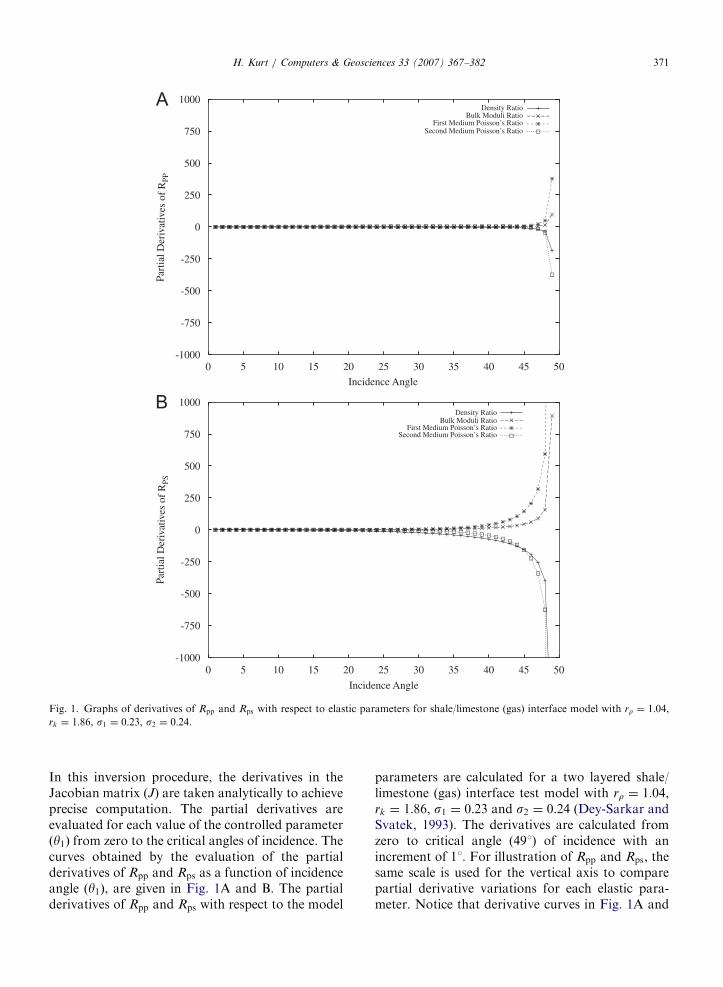
Fig. 1. Graphs of derivatives of Rpp and Rps with respect to elastic parameters for shale/limestone (gas) interface model with rr ¼ 1:04,rk ¼ 1:86, s1 ¼ 0:23, s2 ¼ 0:24.

H. Kurt / Computers & Geosciences 33 (2007) 367–382 371

In this inversion procedure, the derivatives in theJacobian matrix (J) are taken analytically to achieveprecise computation. The partial derivatives areevaluated for each value of the controlled parameterðy1Þ from zero to the critical angles of incidence. Thecurves obtained by the evaluation of the partialderivatives of Rpp and Rps as a function of incidenceangle (y1Þ, are given in Fig. 1A and B. The partialderivatives of Rpp and Rps with respect to the model

parameters are calculated for a two layered shale/limestone (gas) interface test model with rr ¼ 1:04,rk ¼ 1:86, s1 ¼ 0:23 and s2 ¼ 0:24 (Dey-Sarkar andSvatek, 1993). The derivatives are calculated fromzero to critical angle (491) of incidence with anincrement of 11. For illustration of Rpp and Rps, thesame scale is used for the vertical axis to comparepartial derivative variations for each elastic para-meter. Notice that derivative curves in Fig. 1A and

ARTICLE IN PRESS

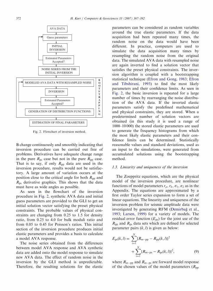
Fig. 2. Flowchart of inversion method.

H. Kurt / Computers & Geosciences 33 (2007) 367–382372

B change continuously and smoothly indicating thatinversion procedure can be carried out free ofproblems. Derivatives have adequate change rangein the pure Rps case but not in the pure Rpp case.That is to say, if only Rpp data are used in theinversion procedure, results would not be satisfac-tory. A large amount of variation occurs at theposition close to the critical angle for both Rpp andRps derivative graphics. This shows that the datamust have as wide angles as possible.

As seen in the flowchart of the inversionprocedure in Fig. 2, synthetic AVA data and initialguess parameters are provided to the GLI to get aninitial solution vector satisfying the preset physicalconstraints. The probable values of physical con-straints are changing from 0.25 to 1.5 for densityratio, from 0.25 to 4.0 for bulk moduli ratio andfrom 0.05 to 0.45 for Poisson’s ratios. This initialsection of the inversion procedure produces initialelastic parameters and provides a basis to calculatea model AVA response.

The noise series obtained from the differencesbetween model AVA response and AVA syntheticdata are added onto the model response to simulatenew AVA data. The effect of random noise in theinversion by the GLI method is unpredictable.Therefore, the resulting solutions for the elastic

parameters can be considered as random variablesaround the true elastic parameters. If the dataacquisition had been repeated many times, therandom noise on the data would have beendifferent. In practice, computers are used tosimulate the data acquisition many times byresampling the random noise from the originaldata. The simulated AVA data with resampled noiseare again inverted to find a solution vector thatsatisfies the preset physical constraints. The inver-sion algorithm is coupled with a bootstrappingstatistical technique (Efron and Gong, 1983; Efronand Tibshirani, 1993) to find the most likelyparameters and their confidence limits. As seen inFig. 2, the basic inversion is repeated for a largenumber of times by rearranging the noise distribu-tion of the AVA data. If the inverted elasticparameters satisfy the predefined mathematicaland physical constraints, they are stored. When apredetermined number of solution vectors areobtained (in this study it is used a range of1000–10 000) the stored elastic parameters are usedto generate the frequency histograms from whichthe most likely elastic parameters and their con-fidence limits can be determined. Statisticallyreasonable values and standard deviations, used asan input to the simulations, were generated fromaccumulated solutions using the bootstrappingmethod.

1.3. Linearity and uniqueness of the inversion

The Zoeppritz equations, which are the physicalmodel of the inversion procedure, are nonlinearfunctions of model parameters rr, rk, s1, s2 as in theAppendix. The equations are approximated by afirst order Taylor series expansion to form a set oflinear equations. The linearity and uniqueness of theinversion problem for seismic amplitude data wereinvestigated by generating RFM (Demirbag et al.,1993; Larsen, 1999) for a variety of models. Theresidual error function ðEpsÞ for the joint use of theRpp and Rps data sets which are defined for selectedparameter pairs ðk; lÞ is given as below:

Epsðk; lÞ ¼XN

i¼1

fRm�pp � Rppðk; lÞg2

þXN

i¼1

fRm�ps � Rpsðk; lÞg2, ð9Þ

where Rm�pp and Rm�ps are forward model responseof the chosen values of the model parameters (Rpp


and Rps values from the Zoeppritz equations).Rppðk; lÞ and Rpsðk; lÞ are the response of the samefunction to different values of the desired parameterpair ðk; lÞ. Epsðk; lÞ is evaluated for all incidence

2.1

2.2

2.3

2.4

2.5

2.6

2.7

2.8

2.9

0.15 0.20 0.25 0.30 0.35

2.1

2.2

2.3

2.4

2.5

2.6

2.7

2.8

2.9

1.00 1.05 1.10 1.15 1.20

Den

sity

Rat

io

Den

sity

Rat

io

Bul

k M

odul

i Rat

ioB

ulk

Mod

uli R

atio

Bul

k M

odul

i Rat

ioFi

rst M

ediu

m P

oiss

on’s

Rat

io

Density Ratio

1.00

1.05

1.10

1.15

1.20

0.15 0.20 0.25 0.30 0.35

First Medium Poisson’s Ratio


A B

C D

E F

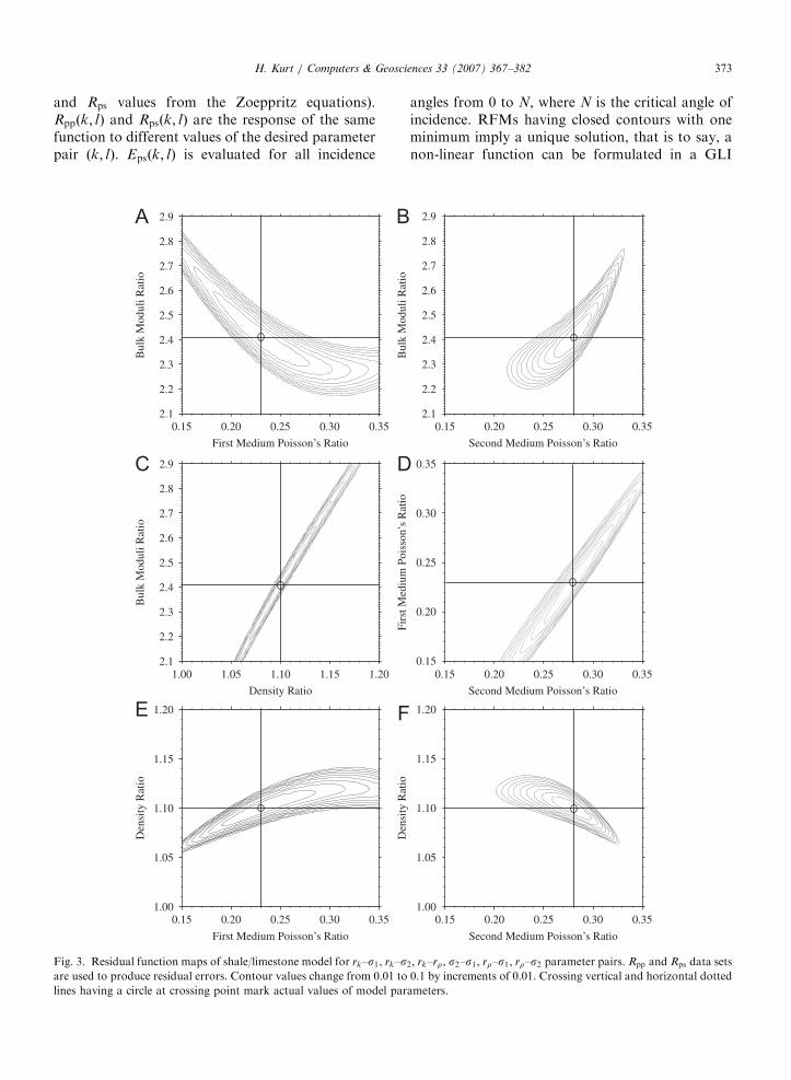
Fig. 3. Residual function maps of shale/limestone model for rk–s1, rk–sare used to produce residual errors. Contour values change from 0.01 to

lines having a circle at crossing point mark actual values of model par

angles from 0 to N, where N is the critical angle ofincidence. RFMs having closed contours with oneminimum imply a unique solution, that is to say, anon-linear function can be formulated in a GLI

2.1

2.2

2.3

2.4

2.5

2.6

2.7

2.8

2.9

0.15 0.20 0.25 0.30 0.35

1.00

1.05

1.10

1.15

1.20

0.15 0.20 0.25 0.30 0.35

0.15

0.20

0.25

0.30

0.35

0.15 0.20 0.25 0.30 0.35

Second Medium Poisson’s Ratio



2, rk–rr, s2–s1, rr–s1, rr–s2 parameter pairs. Rpp and Rps data sets

0.1 by increments of 0.01. Crossing vertical and horizontal dotted

ameters.

ARTICLE IN PRESS

Bul

k M

odul

i Rat

io


2.1

2.2

2.3

2.4

2.5

2.6

2.7

2.8

2.9

0.15 0.20 0.25 0.30 0.35

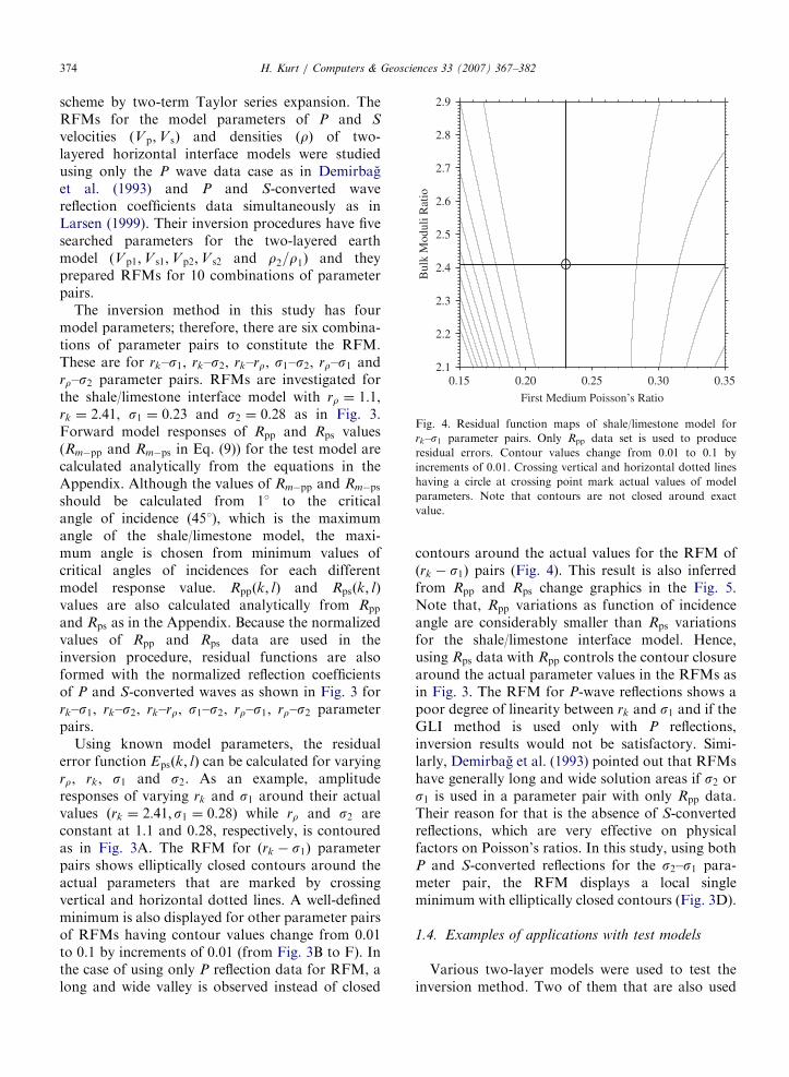
Fig. 4. Residual function maps of shale/limestone model for

rk–s1 parameter pairs. Only Rpp data set is used to produce

residual errors. Contour values change from 0.01 to 0.1 by

increments of 0.01. Crossing vertical and horizontal dotted lines

having a circle at crossing point mark actual values of model

parameters. Note that contours are not closed around exact

value.


scheme by two-term Taylor series expansion. TheRFMs for the model parameters of P and S

velocities ðVp;V sÞ and densities ðrÞ of two-layered horizontal interface models were studiedusing only the P wave data case as in Demirbaget al. (1993) and P and S-converted wavereflection coefficients data simultaneously as inLarsen (1999). Their inversion procedures have fivesearched parameters for the two-layered earthmodel (Vp1;V s1;Vp2;V s2 and r2=r1) and theyprepared RFMs for 10 combinations of parameterpairs.

The inversion method in this study has fourmodel parameters; therefore, there are six combina-tions of parameter pairs to constitute the RFM.These are for rk–s1, rk–s2, rk–rr, s1–s2, rr–s1 andrr–s2 parameter pairs. RFMs are investigated forthe shale/limestone interface model with rr ¼ 1:1,rk ¼ 2:41, s1 ¼ 0:23 and s2 ¼ 0:28 as in Fig. 3.Forward model responses of Rpp and Rps values(Rm�pp and Rm�ps in Eq. (9)) for the test model arecalculated analytically from the equations in theAppendix. Although the values of Rm�pp and Rm�ps

should be calculated from 1� to the criticalangle of incidence (451), which is the maximumangle of the shale/limestone model, the maxi-mum angle is chosen from minimum values ofcritical angles of incidences for each differentmodel response value. Rppðk; lÞ and Rpsðk; lÞvalues are also calculated analytically from Rpp

and Rps as in the Appendix. Because the normalizedvalues of Rpp and Rps data are used in theinversion procedure, residual functions are alsoformed with the normalized reflection coefficientsof P and S-converted waves as shown in Fig. 3 forrk–s1, rk–s2, rk–rr, s1–s2, rr–s1, rr–s2 parameterpairs.

Using known model parameters, the residualerror function Epsðk; lÞ can be calculated for varyingrr, rk, s1 and s2. As an example, amplituderesponses of varying rk and s1 around their actualvalues ðrk ¼ 2:41;s1 ¼ 0:28Þ while rr and s2 areconstant at 1.1 and 0.28, respectively, is contouredas in Fig. 3A. The RFM for ðrk � s1Þ parameterpairs shows elliptically closed contours around theactual parameters that are marked by crossingvertical and horizontal dotted lines. A well-definedminimum is also displayed for other parameter pairsof RFMs having contour values change from 0.01to 0.1 by increments of 0.01 (from Fig. 3B to F). Inthe case of using only P reflection data for RFM, along and wide valley is observed instead of closed

contours around the actual values for the RFM ofðrk � s1Þ pairs (Fig. 4). This result is also inferredfrom Rpp and Rps change graphics in the Fig. 5.Note that, Rpp variations as function of incidenceangle are considerably smaller than Rps variationsfor the shale/limestone interface model. Hence,using Rps data with Rpp controls the contour closurearound the actual parameter values in the RFMs asin Fig. 3. The RFM for P-wave reflections shows apoor degree of linearity between rk and s1 and if theGLI method is used only with P reflections,inversion results would not be satisfactory. Simi-larly, Demirbag et al. (1993) pointed out that RFMshave generally long and wide solution areas if s2 ors1 is used in a parameter pair with only Rpp data.Their reason for that is the absence of S-convertedreflections, which are very effective on physicalfactors on Poisson’s ratios. In this study, using bothP and S-converted reflections for the s2–s1 para-meter pair, the RFM displays a local singleminimum with elliptically closed contours (Fig. 3D).

1.4. Examples of applications with test models

Various two-layer models were used to test theinversion method. Two of them that are also used

ARTICLE IN PRESS

Ref

lect

ion

Coe

ffic

ient

s of

P a

nd C

onve

rted

S W

ave

-0.2

-0.1

0

0.1

0.2

0.3

0.4

0.5

0.6

0.7

0.8

0 5 10 15 20 25 30 35 40 45 50

1 shale/limestone2 shale/limestone (gas)

Angle of Incidence

1(P)

1(S)

2(P)

2(S)

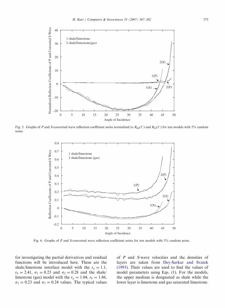
Fig. 6. Graphs of P and S-converted wave reflection coefficient series for test models with 5% random noise.

1(P)

1(S)

-20

-10

0

10

20

30

40

0 5 10 15 20 25 30 35 40 45 50

Angle of Incidence

Nor

mal

ized

Ref

lect

ion

Coe

ffic

ient

s of

P a

nd C

onve

rted

S W

ave

1 shale/limestone2 shale/limestone(gas)

2(P)

2(S)

Fig. 5. Graphs of P and S-converted wave reflection coefficient series normalized to Rppð1�Þ and Rpsð1

�Þ for test models with 5% random

noise.


for investigating the partial derivatives and residualfunctions will be introduced here. These are theshale/limestone interface model with the rr ¼ 1:1,rk ¼ 2:41, s1 ¼ 0:23 and s2 ¼ 0:28 and the shale/limestone (gas) model with the rr ¼ 1:04, rk ¼ 1:86,s1 ¼ 0:23 and s2 ¼ 0:24 values. The typical values

of P and S-wave velocities and the densities oflayers are taken from Dey-Sarkar and Svatek(1993). Their values are used to find the values ofmodel parameters using Eqs. (1). For the models,the upper medium is designated as shale while thelower layer is limestone and gas saturated limestone.


Although models are chosen from typical petroleumtraps, the inversion code can be used for other typesof earth layer units. Rpp and Rps equations obtainedfrom the Zoeppritz equations for precritical anglesare used to produce a synthetic AVA data set forthe models as in the Appendix. A random noise of5% is added to each of the synthetic Rpp and Rps

data sets to simulate realistic amplitude databefore introducing them to the inversion procedure.The synthetic AVA data for all the models arenormalized to the Rppð1Þ and Rpsð1Þ to get rid of theprobable error effect of the exact values on theamplitudes. In Figs. 5 and 6, normalized andnonnormalized Rpp and Rps reflection coefficientsare displayed together as functions of the incidenceangle from 1� to the critical angle of each model. P

and S-converted wave reflection coefficients calcu-

0.00

1.00

Rel

ativ

e Fr

eque

ncy

1.00 1.05 1.10 1.15 1.20 1.25 1.30 1.35 1.40

Density Ratio

0.00

1.00

Rel

ativ

e Fr

eque

ncy

0.1 0.2 0.3 0.4

First Medium Poisson's Ratio

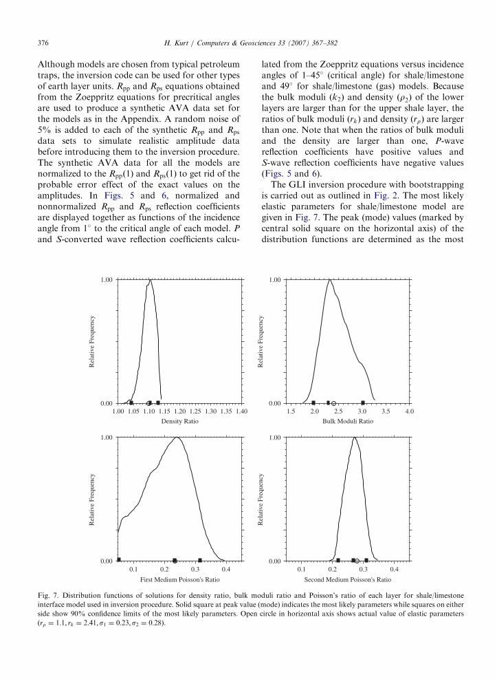
Fig. 7. Distribution functions of solutions for density ratio, bulk mo

interface model used in inversion procedure. Solid square at peak value (

side show 90% confidence limits of the most likely parameters. Open

ðrr ¼ 1:1; rk ¼ 2:41;s1 ¼ 0:23; s2 ¼ 0:28Þ.

lated from the Zoeppritz equations versus incidenceangles of 1–45� (critical angle) for shale/limestoneand 49� for shale/limestone (gas) models. Becausethe bulk moduli ðk2Þ and density ðr2Þ of the lowerlayers are larger than for the upper shale layer, theratios of bulk moduli ðrkÞ and density ðrrÞ are largerthan one. Note that when the ratios of bulk moduliand the density are larger than one, P-wavereflection coefficients have positive values andS-wave reflection coefficients have negative values(Figs. 5 and 6).

The GLI inversion procedure with bootstrappingis carried out as outlined in Fig. 2. The most likelyelastic parameters for shale/limestone model aregiven in Fig. 7. The peak (mode) values (marked bycentral solid square on the horizontal axis) of thedistribution functions are determined as the most

0.00

1.00

1.5 2.0 2.5 3.0 3.5 4.0

Bulk Moduli Ratio

0.00

1.00

Rel

ativ

e Fr

eque

ncy

0.1 0.2 0.3 0.4

Second Medium Poisson's Ratio

Rel

ativ

e Fr

eque

ncy

duli ratio and Poisson’s ratio of each layer for shale/limestone

mode) indicates the most likely parameters while squares on either

circle in horizontal axis shows actual value of elastic parameters

ARTICLE IN PRESS

0.00

1.00

0.1 0.2 0.3 0.4


0.00

1.00

0.1 0.2 0.3 0.4 0.5


0.00

1.00

Rel

ativ

e Fr

eque

ncy

Rel

ativ

e Fr

eque

ncy

Rel

ativ

e Fr

eque

ncy

Rel

ativ

e Fr

eque

ncy

1.00 1.05 1.10 1.15 1.20 1.25 1.30 1.35 1.40

Density Ratio

0.00

1.00

1.5 2.0 2.5 3.0 3.5 4.0

Bulk Moduli Ratio

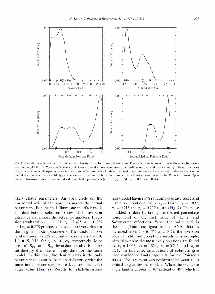
Fig. 8. Distribution functions of solutions for density ratio, bulk moduli ratio and Poisson’s ratio of second layer for shale/limestone

interface model if only P wave reflection coefficients are used in inversion procedure. Solid square at peak value (mode) indicates the most

likely parameters while squares on either side show 90% confidence limits of the most likely parameters. Because peak value and maximum

confidence limits of the most likely parameters are very close, solid squares are shown almost at same location for Poisson’s ratios. Open

circle in horizontal axis shows actual value of elastic parameters ðrr ¼ 1:1; rk ¼ 2:41;s1 ¼ 0:23; s2 ¼ 0:28Þ.


likely elastic parameters. An open circle on thehorizontal axis of the graphics marks the actualparameters. For the shale/limestone interface mod-el, distribution solutions show that inversionestimates are almost the actual parameters. Inver-sion results with rr ¼ 1:101, rk ¼ 2:425, s1 ¼ 0:225and s2 ¼ 0:278 produce values that are very close tothe original model parameters. The random noiselevel is chosen as 5% and initial parameters are 1.4,1.9, 0.19, 0.18, for rr, rk, s1, s2, respectively. Jointuse of Rpp and Rps inversion results is moresatisfactory then the Rpp only data for the samemodel. In this case, the density ratio is the onlyparameter that can be found satisfactorily with thesame initial parameters, noise level and incidenceangle value (Fig. 8). Results for shale/limestone

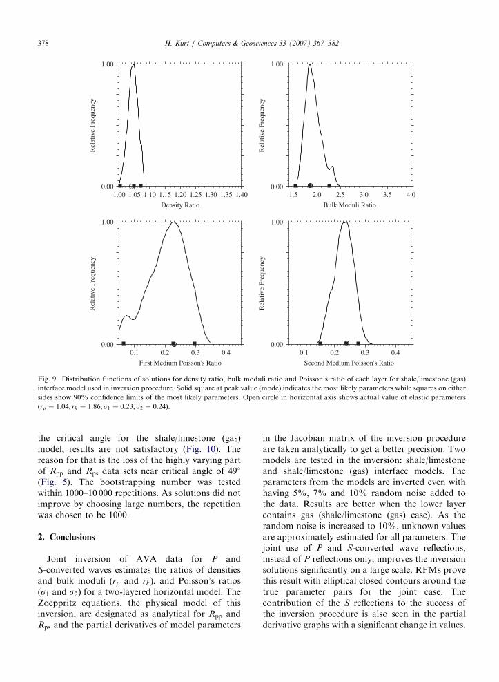
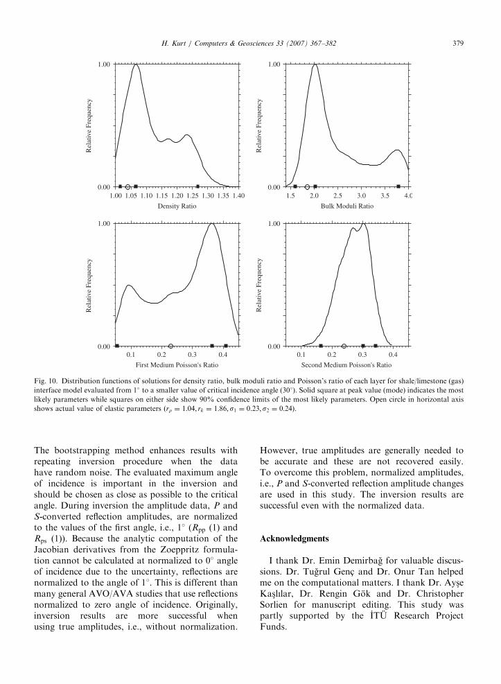
(gas) model having 5% random noise give successfulinversion solutions with rr ¼ 1:045, rk ¼ 1:892,s1 ¼ 0:216 and s2 ¼ 0:232 values (Fig. 9). The noiseis added to data by taking the desired percentagenoise level of the first value of the P andS-converted reflections. When the noise level inthe shale/limestone (gas) model AVA data isincreased from 5% to 7% and 10%, the inversioncode can still find acceptable results. For example,with 10% noise the most likely solutions are foundas rr ¼ 1:008, rk ¼ 1:824, s1 ¼ 0:243 and s2 ¼0:242. In this case, distributions of solutions givewide confidence limits especially for the Poisson’sratios. The inversion was performed between 1� tocritical angles for the models. When the incidenceangle limit is chosen as 30� instead of 49�, which is

ARTICLE IN PRESS

0.00

1.00

0.1 0.2 0.3 0.4


0.00

1.00

0.1 0.2 0.3 0.4


0.00

1.00

Rel

ativ

e Fr

eque

ncy

Rel

ativ

e Fr

eque

ncy

Rel

ativ

e Fr

eque

ncy

Rel

ativ

e Fr

eque

ncy

1.00 1.05 1.10 1.15 1.20 1.25 1.30 1.35 1.40

Density Ratio

0.00

1.00

1.5 2.0 2.5 3.0 3.5 4.0

Bulk Moduli Ratio

Fig. 9. Distribution functions of solutions for density ratio, bulk moduli ratio and Poisson’s ratio of each layer for shale/limestone (gas)

interface model used in inversion procedure. Solid square at peak value (mode) indicates the most likely parameters while squares on either

sides show 90% confidence limits of the most likely parameters. Open circle in horizontal axis shows actual value of elastic parameters

ðrr ¼ 1:04; rk ¼ 1:86;s1 ¼ 0:23;s2 ¼ 0:24Þ.


the critical angle for the shale/limestone (gas)model, results are not satisfactory (Fig. 10). Thereason for that is the loss of the highly varying partof Rpp and Rps data sets near critical angle of 49�

(Fig. 5). The bootstrapping number was testedwithin 1000–10 000 repetitions. As solutions did notimprove by choosing large numbers, the repetitionwas chosen to be 1000.

2. Conclusions

Joint inversion of AVA data for P andS-converted waves estimates the ratios of densitiesand bulk moduli (rr and rk), and Poisson’s ratios(s1 and s2) for a two-layered horizontal model. TheZoeppritz equations, the physical model of thisinversion, are designated as analytical for Rpp andRps and the partial derivatives of model parameters

in the Jacobian matrix of the inversion procedureare taken analytically to get a better precision. Twomodels are tested in the inversion: shale/limestoneand shale/limestone (gas) interface models. Theparameters from the models are inverted even withhaving 5%, 7% and 10% random noise added tothe data. Results are better when the lower layercontains gas (shale/limestone (gas) case). As therandom noise is increased to 10%, unknown valuesare approximately estimated for all parameters. Thejoint use of P and S-converted wave reflections,instead of P reflections only, improves the inversionsolutions significantly on a large scale. RFMs provethis result with elliptical closed contours around thetrue parameter pairs for the joint case. Thecontribution of the S reflections to the success ofthe inversion procedure is also seen in the partialderivative graphs with a significant change in values.

ARTICLE IN PRESS

0.00

1.00

0.1 0.2 0.3 0.4


0.00

1.00

0.1 0.2 0.3 0.4


0.00

1.00

Rel

ativ

e Fr

eque

ncy

Rel

ativ

e Fr

eque

ncy

Rel

ativ

e Fr

eque

ncy

Rel

ativ

e Fr

eque

ncy

1.00 1.05 1.10 1.15 1.20 1.25 1.30 1.35 1.40

Density Ratio

0.00

1.00

1.5 2.0 2.5 3.0 3.5 4.0

Bulk Moduli Ratio

Fig. 10. Distribution functions of solutions for density ratio, bulk moduli ratio and Poisson’s ratio of each layer for shale/limestone (gas)

interface model evaluated from 1� to a smaller value of critical incidence angle (301). Solid square at peak value (mode) indicates the most

likely parameters while squares on either side show 90% confidence limits of the most likely parameters. Open circle in horizontal axis

shows actual value of elastic parameters ðrr ¼ 1:04; rk ¼ 1:86; s1 ¼ 0:23;s2 ¼ 0:24Þ.


The bootstrapping method enhances results withrepeating inversion procedure when the datahave random noise. The evaluated maximum angleof incidence is important in the inversion andshould be chosen as close as possible to the criticalangle. During inversion the amplitude data, P andS-converted reflection amplitudes, are normalizedto the values of the first angle, i.e., 1� (Rpp (1) andRps (1)). Because the analytic computation of theJacobian derivatives from the Zoeppritz formula-tion cannot be calculated at normalized to 0� angleof incidence due to the uncertainty, reflections arenormalized to the angle of 11. This is different thanmany general AVO/AVA studies that use reflectionsnormalized to zero angle of incidence. Originally,inversion results are more successful whenusing true amplitudes, i.e., without normalization.

However, true amplitudes are generally needed tobe accurate and these are not recovered easily.To overcome this problem, normalized amplitudes,i.e., P and S-converted reflection amplitude changesare used in this study. The inversion results aresuccessful even with the normalized data.

Acknowledgments

I thank Dr. Emin Demirbag for valuable discus-sions. Dr. Tugrul Genc- and Dr. Onur Tan helpedme on the computational matters. I thank Dr. Ays-eKas-lılar, Dr. Rengin Gok and Dr. ChristopherSorlien for manuscript editing. This study waspartly supported by the ITU Research ProjectFunds.


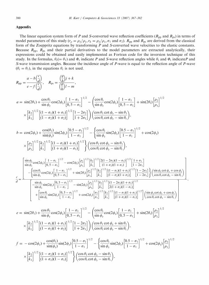
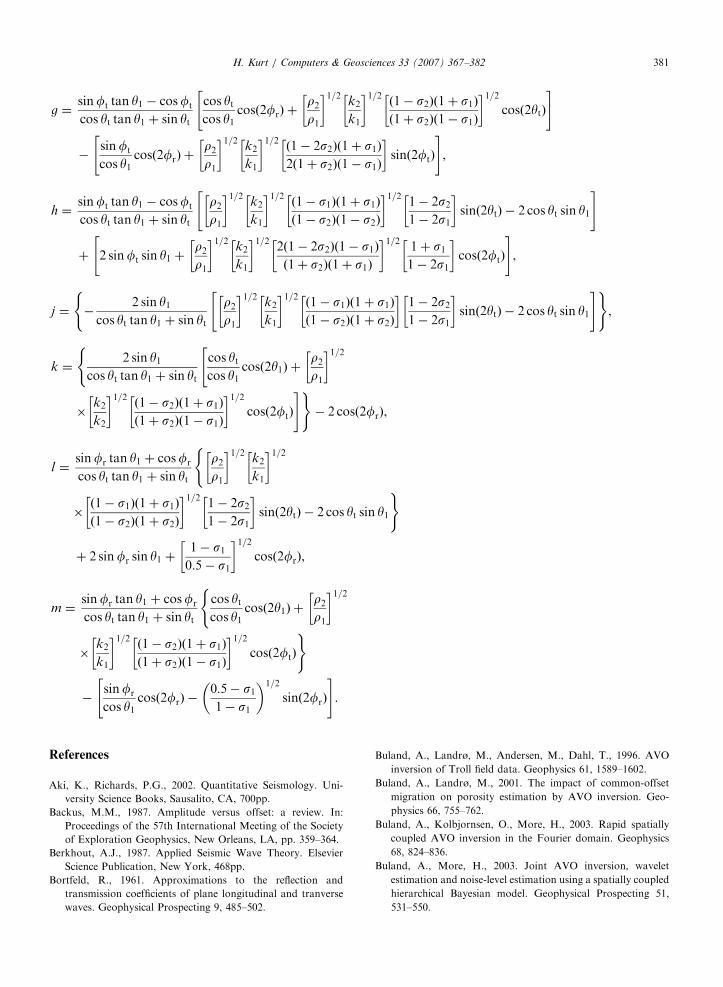
Appendix

The linear equation system form of P and S-converted wave reflection coefficients (Rpp and Rps) in terms ofmodel parameters of this study (rr ¼ r2=r1; rk ¼ r2=r1;s1 and s2). Rpp and Rps are derived from the classicalform of the Zoeppritz equations by transforming P and S-converted wave velocities to the elastic constants.Because Rpp, Rps and their partial derivatives to the model parameters are extracted analytically, theirexpressions could be obtained and easily implemented as Fortran code for the inversion technique of thisstudy. In the formulas, yrð¼ y1Þ and Fr indicate P and S-wave reflection angles while yt and Ft indicateP andS-wave transmission angles. Because the incidence angle of P-wave is equal to the reflection angle of P-waveðyr ¼ y1Þ, in the equations yr is not used.

Rpp ¼

a� bc

d

� �e� f

c

d

� � ; Rps ¼

g

h

� �j þ k

g

h

� �l �m

,

a ¼ sinð2y1Þ þcos y1sinfr

cosð2frÞ1� s10; 5� s1

� �1=2�

cos ytsinfr


� �þ sinð2ytÞ

r2r1

� �1=2

�k2

k1

� �1=2ð1� s1Þð1þ s1Þð1� s2Þð1þ s2Þ

� �1=21� 2s21þ 2s1

� �!cos y1 cotfr � sin y1cos yt cotfr � sin yt

� �,

b ¼ cosð2frÞ þcosðy1ÞsinðfrÞ

sinð2frÞ0:5� s11� s1

� �1=2�

cos ytsinfr


� �1=2þ cosð2ftÞ

(

�r2r1

� �1=2k2

k1

� �1=2ð1� s2Þð1þ s1Þð1þ s2Þð1� s1Þ

� �1=2)cos y1 cotfr � sin y1cos yt cotfr � sin yt

� �,

c

d¼

sinft

sinfr


� �1=2� cosð2ftÞ

r2r1

� �1=2k2

k1

� �1=22ð1� 2s2Þð1� s1Þð1þ s2Þð1þ s1Þ

� �1=21þ s11� 2s1

� �

�cos ytsinfr


� �1=2þ sinð2ytÞ

r2r1

� �1=2k2

k1


� �1=21� 2s21� 2s1

� �( )sinft cotfr þ cosft

cos yt cotfr � sin yt

� �2666664

3777775

�sinft

sinfr

sinð2frÞ0; 5� s11� s1

� �1=2� sinð2ftÞ

r2r1

� �1=2k2

k1

� �1=2ð1� 2s2Þð1þ s1Þ2ð1þ s2Þð1� s1Þ

� �1=2

þcos ytsinfr

sinð2frÞ0; 5� s11� s1


s2s1

� �1=2k2

k1


� �1=2" #sinft cotfr þ cosft

cos yt cotfr � sin yt

� �2666664

3777775

,

e ¼ sinð2y1Þ þcos y1sinfr


� �1=2�

cos ytsinfr


� �þ sinð2ytÞ

r2r1

� �1=2

�k2

k1


� �1=21� 2s21þ 2s1

� �!cos y1 cotfr þ sin y1cos yt cotfr � sin yt

� �,

f ¼ � cosð2frÞ þcosðy1ÞsinðfrÞ


� �1=2�

cos ytsinfr



r2r1

� �1=2(

�k2

k1


� �1=2)cos y1 cotfr � sin y1cos yt cotfr � sin yt

� �,


g ¼sinft tan y1 � cosft

cos yt tan y1 þ sin yt

cos ytcos y1

cosð2frÞ þr2r1

� �1=2k2

k1


� �1=2cosð2ytÞ

" #

�sinft

cos y1cosð2frÞ þ

r2r1

� �1=2k2

k1

� �1=2ð1� 2s2Þð1þ s1Þ2ð1þ s2Þð1� s1Þ

� �sinð2ftÞ

" #,

h ¼sinft tan y1 � cosft


r2r1

� �1=2k2

k1

� �1=2ð1� s1Þð1þ s1Þð1� s2Þð1� s2Þ

� �1=21� 2s21� 2s1

� �sinð2ytÞ � 2 cos yt sin y1

" #

þ 2 sinft sin y1 þr2r1

� �1=2k2

k1

� �1=22ð1� 2s2Þð1� s1Þð1þ s2Þð1þ s1Þ

� �1=21þ s11� 2s1

� �cosð2ftÞ

" #,

j ¼ �2 sin y1


r2r1

� �1=2k2

k1


� �1� 2s21� 2s1


" #( ),

k ¼2 sin y1


cos ytcos y1

cosð2y1Þ þr2r1

� �1=2"(

�k2

k2


� �1=2cosð2ftÞ

#)� 2 cosð2frÞ,

l ¼sinfr tan y1 þ cosfr


r2r1

� �1=2k2

k1

� �1=2(

�ð1� s1Þð1þ s1Þð1� s2Þð1þ s2Þ

� �1=21� 2s21� 2s1


)

þ 2 sinfr sin y1 þ1� s10:5� s1

� �1=2cosð2frÞ,

m ¼sinfr tan y1 þ cosfr


cos ytcos y1

cosð2y1Þ þr2r1

� �1=2(

�k2

k1


� �1=2cosð2ftÞ

)

�sinfr

cos y1cosð2frÞ �

0:5� s11� s1

� �1=2

sinð2frÞ

" #.

References

Aki, K., Richards, P.G., 2002. Quantitative Seismology. Uni-

versity Science Books, Sausalito, CA, 700pp.

Backus, M.M., 1987. Amplitude versus offset: a review. In:

Proceedings of the 57th International Meeting of the Society

of Exploration Geophysics, New Orleans, LA, pp. 359–364.

Berkhout, A.J., 1987. Applied Seismic Wave Theory. Elsevier

Science Publication, New York, 468pp.

Bortfeld, R., 1961. Approximations to the reflection and

transmission coefficients of plane longitudinal and tranverse

waves. Geophysical Prospecting 9, 485–502.

Buland, A., Landrø, M., Andersen, M., Dahl, T., 1996. AVO

inversion of Troll field data. Geophysics 61, 1589–1602.

Buland, A., Landrø, M., 2001. The impact of common-offset

migration on porosity estimation by AVO inversion. Geo-

physics 66, 755–762.

Buland, A., Kolbjornsen, O., More, H., 2003. Rapid spatially

coupled AVO inversion in the Fourier domain. Geophysics

68, 824–836.

Buland, A., More, H., 2003. Joint AVO inversion, wavelet

estimation and noise-level estimation using a spatially coupled

hierarchical Bayesian model. Geophysical Prospecting 51,

531–550.


Carazzone, J.J., Srnka, L.J., 1993. Elastic inversion of Gulf of

Mexico data. In: Castagna, J.P., Backus, M.M. (Eds.), Offset-

Dependent Reflectivity-Theory and Practice of AVO Analy-

sis, Investigations in Geophysics, vol. 8. Society of Explora-

tion Geophysics, Tulsa, OK, pp. 303–313.

Dahl, T., Ursin, B., 1992. Non-linear AVO inversion for a

stack of anelastic layers. Geophysical Prospecting 40,

243–265.

Demirbag, E., C- oruh, C., Costain, J.K., 1993. Inversion of

P-Wave AVO. In: Castagna, J.P., Backus, M.M. (Eds.),

Offset-Dependent Reflectivity-Theory and Practice of AVO

Analysis, Investigations in Geophysics, vol. 8. Society of

Exploration Geophysics, Tulsa, OK, pp. 287–302.

Dey-Sarkar, S.K., Svatek, S.V., 1993. Prestack analysis—an

integrated approach for seismic interpretation in classics

basins. In: Castagna, J.P., Backus, M.M. (Eds.), Offset-

Dependent Reflectivity—Theory and Practice of AVO Ana-

lysis, Investigations in Geophysics, vol. 8. Society of

Exploration Geophysics, Tulsa, OK, pp. 57–77.

Domenico, S.N., 1977. Elastic properties of unconsolidated

porous sand reservoirs. Geophysics 42, 1339–1369.

Efron, B., Gong, G., 1983. A leisurely look at the bootstrap, the

jackknife, and cross-validation. American Statistician 37,

36–48.

Efron, B., Tibshirani, R.J., 1993. An Introduction to the

Bootstrapping. Chapman & Hall, New York, 436pp.

Goodway, B., Chen, T., Downton, J., 1997. Improved AVO fluid

detection and lithology discrimination using Lame petrophy-

sical parameters; ‘‘lr’’, ‘‘mr’’, & ‘‘l=m fluid stack’’, from P and

S inversions. In: Proceedings of the 67th International

Meeting of the Society of Exploration Geophysics, Dallas,

TX, pp. 183–186.

Larsen, J.A., 1999. AVO inversion by simultaneous P–P and

P–S inversion. M.Sc. Thesis, The University of Calgary,

124pp.

Lavaud, B., Kabir, N., Chavent, G., 1999. Pushing AVO

inversion beyond linearized approximation. Journal of

Seismic Exploration 8, 279–302.

Lines, L.R., Treitel, S., 1984. Tutorial: a review of least squares

inversion and its application to geophysical problems.

Geophysical Prospecting 32, 159–186.

Mahob, P.N., Castagna, J.P., Young, R.A., 1999. AVO inversion

of a Gulf of Mexico bright spot—a case study. Geophysics 64,

1480–1491.

Margrave, G.F., Stewart, R.R., Larsen, J.A., 2001. Joint PP and

PS seismic inversion. The Leading Edge 20, 1048–1052.

Ostrander, W.J., 1984. Plane-wave reflection coefficients for gas

sands at nonnormal angles of incidence. Geophysics 49,

1637–1648.

Pigott, J.D., Shrestha, R.K., Warwick, R.A., 1989. Young

modulus from AVO inversion. In: Proceedings of the 59th

International Meeting of the Society of Exploration Geo-

physics, vol. 2, Dallas, TX, pp. 832–835.

Riedel, M., Dosso, S.E., Beran, L., 2003. Uncertainty estimation

for amplitude variation with offset (AVO) inversion. Geo-

physics 68, 1485–1496.

Rutherford, S.R., Williams, R.H., 1989. Amplitude-versus-offset

variations in gas sands. Geophysics 54, 680–688.

Sheriff, R.E., Geldart, L.P., 1995. Exploration Seismology.

Cambridge University Press, New York, 592pp.

Shuey, R.T., 1985. A simplification of the Zoeppritz equations.

Geophysics 50, 609–614.

Stewart, R.R., Zhang, Q., Guthoff, F., 1995. Relationships

among elastic-wave values: Rpp, Rps, Rss, Vp, Vs, k, s and r.The CREWES Project Research Report # 7, The University

of Calgary, 9pp.

Wang, Y., 1999. Simultaneous inversion for model geometry and

elastic parameters. Geophysics 64, 182–190.

Zoeppritz, K., 1919. On reflection and propagation of seismic

waves. Gottinger Nachrichten I, 66–84.

Documents

Joint inversion of AVA data for elastic parameters by