Joint integrative analysis of multiple data sources with

Joint integrative analysis of multiple data sourceswith correlated vector outcomes

Emily C. HectorDepartment of Statistics

North Carolina State Universityand

Peter X.-K. SongDepartment of Biostatistics

University of Michigan

Abstract

We propose a distributed quadratic inference function framework to jointly estimate regres-sion parameters from multiple potentially heterogeneous data sources with correlated vectoroutcomes. The primary goal of this joint integrative analysis is to estimate covariate effectson all outcomes through a marginal regression model in a statistically and computationallyefficient way. We develop a data integration procedure for statistical estimation and inferenceof regression parameters that is implemented in a fully distributed and parallelized computa-tional scheme. To overcome computational and modeling challenges arising from the high-dimensional likelihood of the correlated vector outcomes, we propose to analyze each datasource using Qu et al. (2000)’s quadratic inference functions, and then to jointly reestimateparameters from each data source by accounting for correlation between data sources usinga combined meta-estimator in a similar spirit to Hansen (1982)’s generalised method of mo-ments. We show both theoretically and numerically that the proposed method yields efficiencyimprovements and is computationally fast. We illustrate the proposed methodology with thejoint integrative analysis of the association between smoking and metabolites in a large multi-cohort study and provide an R package for ease of implementation.

Keywords: Data integration, Generalised method of moments, Parallel computing, Quadratic in-ference function, Scalable computing, Seemingly unrelated regression.

1

arX

iv:2

011.

1499

6v1

[st

at.M

E]

30

Nov

202

0

1 Introduction

Data integration methods have drawn increasing attention with the availability of massive data from

multiple sources, with proposed methods spanning the gamut from the frequentist confidence dis-

tribution approach (Xie et al., 2011; Xie and Singh, 2013) to Bayesian hierarchical models (Smith

et al., 1995), as well as several generalisations of Glass (1976)’s meta-analysis (Ioannidis, 2006;

DerSimonian and Laird, 2015; Kundu et al., 2019). This paper is substantially motivated by the

analysis of the effect of smoking on metabolites that are upstream determinants of cardiovascu-

lar health. We consider the analysis of four independent cohorts that quantify metabolites across

multiple dependent metabolic sub-pathways in the Metabolic Syndrome in Men (METSIM) study

(Laakso et al., 2017). We refer to each cohort and sub-pathway as a data source. Of interest is

a pathway-specific joint integrative regression analysis of all independent cohorts and dependent

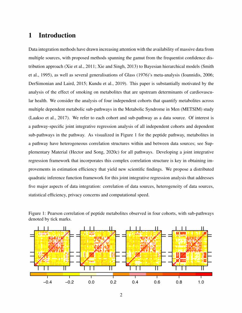
sub-pathways in the pathway. As visualized in Figure 1 for the peptide pathway, metabolites in

a pathway have heterogeneous correlation structures within and between data sources; see Sup-

plementary Material (Hector and Song, 2020c) for all pathways. Developing a joint integrative

regression framework that incorporates this complex correlation structure is key in obtaining im-

provements in estimation efficiency that yield new scientific findings. We propose a distributed

quadratic inference function framework for this joint integrative regression analysis that addresses

five major aspects of data integration: correlation of data sources, heterogeneity of data sources,

statistical efficiency, privacy concerns and computational speed.

Figure 1: Pearson correlation of peptide metabolites observed in four cohorts, with sub-pathwaysdenoted by tick marks.

−0.4 −0.2 0.0 0.2 0.4 0.6 0.8 1.0

2

Recent work has primarily focused on synthesizing evidence from independent data sources,

as in Claggett et al. (2014) and Yang et al. (2014). In practice, however, studies may collect

correlated outcomes from different structural modalities, such as high-dimensional longitudinal

phenotypes, pathway-networked omics biomarkers, or brain imaging measurements, which col-

lectively form one high-dimensional correlated response vector for each participant. Of interest is

conducting inference integrated not only over the independent data sources but also over the struc-

turally correlated outcomes. High-order moments of complex high-dimensional correlated data

may be difficult to model or handle computationally, which has led many to use working indepen-

dence assumptions at the cost of statistical efficiency, resulting in potentially misleading statistical

inference; see for example the composite likelihood approach in Caragea and Smith (2007) and

Varin (2008). Hector and Song (2020b) proposes a method to account for correlation between data

sources without specifying a full parametric model, but their method is burdened by the estima-

tion of a high-dimensional parameter related to the second-order moments, whose dimension can

rapidly increase and exceed the sample size as the number of data sources increases. To relieve this

burden, we propose a fast and efficient approach that avoids estimation of parameters in second-

order moments with no loss of statistical efficiency.

Traditional data integration methods, such as meta-analysis and the confidence distribution ap-

proach, frequently assume parameter or even likelihood homogeneity across data sources, which

often does not hold in practice. Data source heterogeneity can stem from differences in popula-

tions, study design, or associations, and can result in first- and higher-order moment heterogeneity.

On the other hand, seemingly unrelated regression (Zellner, 1962) can be inefficient when some

parameters are homogeneous. One approach to dealing with first-order moment heterogeneity is

to include data source-specific random effects, which can be inefficient and may induce misspec-

ified correlation. Another approach is to allow cohort-specific fixed-effects, as in Lin and Zeng

(2010); Liu et al. (2015); Hector and Song (2020b). In the current literature there is a lack of

computationally fast and statistically efficient methods to handle high-dimensional second- and

higher-order moment parameters, which are regarded as nuisance parameters in a correlated data

integrative setting. With only one data source, the quadratic inference function (Qu et al., 2000)

is widely used to estimate regression parameters in first-order moments while avoiding estima-

tion of second- and higher-order moments. Thus, the quadratic inference function minimizes the

3

excessive burden of handling nuisance parameters. Our proposed distributed quadratic inference

functions estimate regression parameters in mean models for each data source, thereby avoiding

estimation of nuisance parameters in higher-order moments, and linearly updates the regression

parameters according to different heterogeneity patterns across data sources. Not only does our

approach combine the strengths from both meta-analysis and seemingly unrelated regression, but

it is more flexible than these two methods.

For privacy reasons we may not have access to individual level data when integrating correlated

data sources, in which case it becomes imperative to develop methods that can be implemented

in a computationally distributed fashion. Even with access to individual level data, distributed al-

gorithms are often preferred for their ability to significantly reduce the computational burden of

traditional inference methods (Jordan, 2013; Fan et al., 2014). There is a need for distributed meth-

ods able to handle parameter heterogeneity for computationally and statistically efficient inference

with multiple correlated data sources.

Our proposed distributed quadratic inference function approach estimates mean parameters for

cohort- and outcome-specific models in the integrative analysis of correlated outcome vectors

while avoiding estimation of second-order moments. It yields statistically efficient estimation

within a broad class of models. Cohort- and outcome-specific models are then selectively com-

bined via a meta-estimator similar in spirit to Hansen (1982)’s generalised method of moments

according to some characterization of data heterogeneity. This new method has two major advan-

tages over existing methods: the integrated estimator does not require access to individual-level

data, and it can be computed non-iteratively to minimise computational costs.

The paper is organized as follows. In Section 2 we briefly describe the motivating METSIM study

and regression analysis problem. In Section 3 we describe the proposed joint integrative regression

method. We study the numerical performance of our proposed method through simulations in Sec-

tion 4. The integrative analysis of metabolite sub-pathways in METSIM is given in Section 5. We

conclude with a discussion in Section 6. Theoretical justifications and additional numerical results

are deferred to the Appendices and Supplemental Material (Hector and Song, 2020c) respectively.

4

2 Metabolic Syndrome in Men study

The Metabolic Syndrome in Men study is a population-based study of 10197 Finnish men with

the aim of investigating nongenetic and genetic factors associated with the risk of Type 2 diabetes,

cardiovascular disease, and cardiovascular risk factors (Laakso et al., 2017). The Centers for Dis-

ease Control and Prevention list smoking as a major cause of cardiovascular disease and the 2014

Surgeon General’s Report on smoking and health reported that smoking was responsible for one

of every four deaths from cardiovascular disease. Investigating the association between smoking

and metabolites can provide insight into the etiology of metabolic diseases such as cardiovascular

disease.

Using the Metabolon platform, the Metabolic Syndrome in Men study measured metabolites in

eight pathways in four separate samples of men. Of interest is a regression analysis of the ef-

fect of smoking on metabolites in each of the eight pathways. Due to the complex correlation

structure within and between sub-pathways in a pathway, we focus on a local model specification

within each cohort and sub-pathway, termed a data source, and aim to integrate models across data

sources for a joint integrative regression approach. For each pathway, the effect of smoking is

known a priori to be partially homogeneous across sub-pathways: the regression models for the

sub-pathways can be grouped according to a known partition scheme P that describes the homo-

geneity/heterogeneity pattern of regression coefficients from different sub-pathways. For example,

as illustrated in Figure 2, the effect of smoking on peptide metabolites is homogeneous across the

gamma-glutamyl amino acid, modified peptide, and polypeptide sub-pathways, and heterogeneous

across the acetylated peptide, dipeptide and fibrinogen cleavage peptide sub-pathways. The dimen-

sion of the regression parameter of interest therefore is a function both of the number of covariates

and the number of heterogeneous partitions.

In Section 3 we describe the general framework for estimating pathway-specific regression param-

eters that are partially homogeneous across the independent cohorts and dependent sub-pathways.

For this general framework, we focus on one pathway and refer to each cohort and sub-pathway as

a data source. The application of the proposed method to the METSIM study is revisited in Section

5.

5

3 Distributed and integrated quadratic inference functions

3.1 Model formulation

ConsiderK independent cohorts with respective sample sizes nk, k = 1, . . . , K. In each cohort we

observe J correlated mi,j-element vector outcomes yi,jk = (yi1,jk, . . . , yimi,j ,jk)T , j = 1, . . . , J ,

for each participant i, i = 1, . . . , nk, with xi,jk the corresponding mi,j × p covariate matrix.

Here xi,jk is assumed to be the cohort- and outcome-specific observations on the same vari-

ables across outcomes and cohorts (e.g. age, sex, exposure). Participants are assumed inde-

pendent, and let Σi,k be the covariance matrix of yi,k = (yi,1k, . . . ,yi,Jk)T . We consider the

model E(yir,jk) = hjk(xir,jkθjk), r = 1, . . . ,mi,j , where hjk is a known link function and θjk

is a p × 1 parameter vector of interest. Suppose there exists a known partition P = {Pg}Gg=1,

P a set of disjoint non-empty subsets Pg, of {(j, k)}J,Kj,k=1 such that θjk ≡ θg and hjk ≡ hg for

(j, k) ∈ Pg. There are G unique values of θjk, j = 1, . . . , J , k = 1, . . . , K. Let Pg have cardi-

nality dg such that∑G

g=1 dg = JK. We want to estimate and make inference about the true value

θ0 = (θ0,g)Gg=1 ∈ RGp of θ = (θg)

Gg=1 ∈ RGp based on all JK sources of information.

We give an example from Section 5 to fix ideas. For K = 4 cohorts, we quantify 36 metabolites

from J = 6 peptide sub-pathways: acetylated peptides, dipeptide, fibrinogen cleavage peptide,

gamma-glutamyl amino acid, modified peptides, and polypeptide. Given the biological function

of these sub-pathways, we model the effect of smoking on the peptide metabolites by integrat-

ing its effect over the four cohorts and the latter four sub-pathways, and integrating the effect

of smoking on the first, second and third sub-pathways only over cohorts. This partition corre-

sponds to P = {Pg}4g=1, where P1 = {(1, k)}Kk=1, P2 = {(2, k)}Kk=1, P3 = {(3, k)}Kk=1 and

P4 = {(4, k), (5, k), (6, k)}Kk=1. This partition is visualized in Figure 2.

The proposed method creates a set of moment conditions on θ, with corresponding estimators,

from each data source. We propose an efficient and computationally attractive estimator that lin-

early updates data source-specific estimators by weighting them as a function of their covariance.

We introduce some notation to facilitate the description of the proposed method in sections 3.2

and 3.3. For ease of exposition, we henceforth use the term “cohorts” to refer to the K disjoint

and independent participant groups, “block” to refer to the J correlated vector outcomes. We re-

6

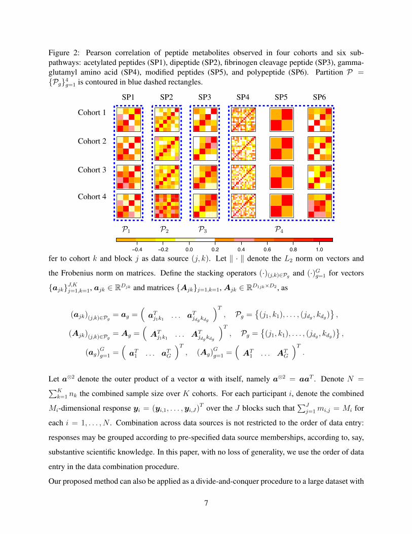
Figure 2: Pearson correlation of peptide metabolites observed in four cohorts and six sub-pathways: acetylated peptides (SP1), dipeptide (SP2), fibrinogen cleavage peptide (SP3), gamma-glutamyl amino acid (SP4), modified peptides (SP5), and polypeptide (SP6). Partition P ={Pg}4

g=1 is contoured in blue dashed rectangles.

Cohort 1

Cohort 2

Cohort 3

Cohort 4

SP1 SP2 SP3 SP4 SP5 SP6

P1 P2 P3 P4

−0.4 −0.2 0.0 0.2 0.4 0.6 0.8 1.0

fer to cohort k and block j as data source (j, k). Let ‖ · ‖ denote the L2 norm on vectors and

the Frobenius norm on matrices. Define the stacking operators (·)(j,k)∈Pg and (·)Gg=1 for vectors

{ajk}J,Kj=1,k=1, ajk ∈ RDjk and matrices {Ajk}j=1,k=1,Ajk ∈ RD1jk×D2 , as

(ajk)(j,k)∈Pg= ag =

(aTj1k1 . . . aTjdgkdg

)T, Pg =

{(j1, k1), . . . , (jdg , kdg)

},

(Ajk)(j,k)∈Pg= Ag =

(ATj1k1

. . . ATjdgkdg

)T, Pg =

{(j1, k1), . . . , (jdg , kdg)

},

(ag)Gg=1 =

(aT1 . . . aTG

)T, (Ag)

Gg=1 =

(AT

1 . . . ATG

)T.

Let a⊗2 denote the outer product of a vector a with itself, namely a⊗2 = aaT . Denote N =∑Kk=1 nk the combined sample size over K cohorts. For each participant i, denote the combined

Mi-dimensional response yi = (yi,1, . . . ,yi,J)T over the J blocks such that∑J

j=1mi,j = Mi for

each i = 1, . . . , N . Combination across data sources is not restricted to the order of data entry:

responses may be grouped according to pre-specified data source memberships, according to, say,

substantive scientific knowledge. In this paper, with no loss of generality, we use the order of data

entry in the data combination procedure.

Our proposed method can also be applied as a divide-and-conquer procedure to a large dataset with

7

N samples on M correlated outcomes. Dividing this large dataset into JK sources of data with

sample size nk and mj-dimensional outcomes yields the above framework with the simplification

Mi = M , mi,j = mj .

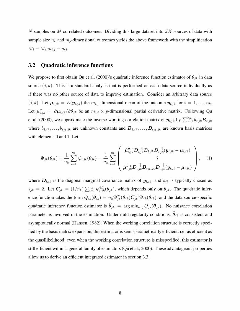
3.2 Quadratic inference functions

We propose to first obtain Qu et al. (2000)’s quadratic inference function estimator of θjk in data

source (j, k). This is a standard analysis that is performed on each data source individually as

if there was no other source of data to improve estimation. Consider an arbitrary data source

(j, k). Let µi,jk = E(yi,jk) the mi,j-dimensional mean of the outcome yi,jk for i = 1, . . . , nk.

Let µθi,jk = ∂µi,jk/∂θjk be an mi,j × p-dimensional partial derivative matrix. Following Qu

et al. (2000), we approximate the inverse working correlation matrix of yi,jk by∑sjk

s=1 bs,jkBs,jk

where b1,jk, . . . , bsjk,jk are unknown constants and B1,jk, . . . ,Bsjk,jk are known basis matrices

with elements 0 and 1. Let

Ψjk(θjk) =1

nk

nk∑i=1

ψi,jk(θjk) =1

nk

nk∑i=1

µθ Ti,jkD

− 12

i,jkB1,jkD− 1

2i,jk(yi,jk − µi,jk)

...

µθ Ti,jkD

− 12

i,jkBsjk,jkD− 1

2i,jk(yi,jk − µi,jk)

, (1)

where Di,jk is the diagonal marginal covariance matrix of yi,jk, and sjk is typically chosen as

sjk = 2. Let Cjk = (1/nk)∑nk

i=1ψ⊗2i,jk(θjk), which depends only on θjk. The quadratic infer-

ence function takes the form Qjk(θjk) = nkΨTjk(θjk)C

−1jk Ψjk(θjk), and the data source-specific

quadratic inference function estimator is θjk = arg minθjk Qjk(θjk). No nuisance correlation

parameter is involved in the estimation. Under mild regularity conditions, θjk is consistent and

asymptotically normal (Hansen, 1982). When the working correlation structure is correctly speci-

fied by the basis matrix expansion, this estimator is semi-parametrically efficient, i.e. as efficient as

the quasilikelihood; even when the working correlation structure is misspecified, this estimator is

still efficient within a general family of estimators (Qu et al., 2000). These advantageous properties

allow us to derive an efficient integrated estimator in section 3.3.

8

3.3 Integrated estimator

Define the cohort indicator δi(k) = 1(participant i is in cohort k) for i = 1, . . . , N , k = 1, . . . , K.

For participant i, let

ψi,g(θ) = {δi(k)ψi,jk(θjk)}(j,k)∈Pg, ψi(θ) = {ψi,g(θ)}Gg=1 .

Then we can define ΨN(θ) = (1/N)∑N

i=1ψi(θ). It is easy to show that

ΨN(θ) =1

N

N∑i=1

[{δi(k)ψi,jk(θjk)}(j,k)∈Pg

]Gg=1

=1

N

[{nkΨjk(θjk)}(j,k)∈Pg

]Gg=1

.

We define a few sample sensitivity matrices. For data source (j, k), define the (psjk)×p-dimensional

sample sensitivity matrix Sjk = −{∇θjkΨjk(θjk)}|θjk=θjk. For the gth set Pg, define Sg =

(nkSjk)(j,k)∈Pg the matrix of stacked sensitivity matrices with row-dimension∑

(j,k)∈Pgpsjk and

column-dimension p. Finally, let S = blockdiag{Sg}Gg=1 the sample sensitivity matrix of ΨN with

row-dimension∑G

g=1

∑(j,k)∈Pg

psjk =∑J,K

j,k=1 psjk and column-dimension Gp.

Let θg = (θjk)(j,k)∈Pg and θlist = (θg)Gg=1. Define ψi(θlist) = [{δi(k)ψi,jk(θjk)}(j,k)∈Pg ]Gg=1.

Let VN = (1/N)∑N

i=1{ψi(θlist)}⊗2 be the sample covariance of ΨN(θ0) with row- and column-

dimension∑J,K

j,k=1 psjk. Then we define the integrated estimator of θ as

θ =(ST V −1

N S)−1

ST V −1N

{(nkSjkθjk)(j,k)∈Pg

}Gg=1

. (2)

Following similar steps to Hector and Song (2020a), we can show this integrated estimator is

asymptotically equivalent to the minimizer of the optimal combination of the moment conditions.

Estimators from different sets Pg may not be combined but still benefit from correlation between

data sources, captured by VN , leading to improved statistical efficiency. This is similar to the gain

in efficiency in seemingly unrelated regression (Zellner, 1962). The closed-form estimator in (2)

depends only on estimators, estimating equations and sample sensitivity matrices from each data

source. It can be implemented in a fully parallelized MapReduce framework, where data sources

are analyzed in parallel on distributed nodes using quadratic inference functions and results from

the separate analyses are sent to a main node to compute the integrated estimator. This procedure is

9

privacy-preserving, since the combination step does not require access to individual level data, and

communication-efficient, since it does not require multiple rounds of communication between the

main and distributed nodes. In addition, it is computationally efficient at each node since nuisance

correlation parameters are not involved in the estimation.

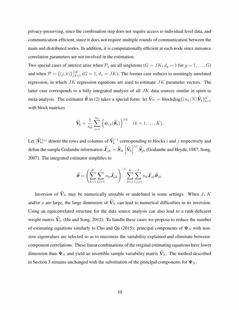
Two special cases of interest arise when Pg are all singletons (G = JK, dg = 1 for g = 1, . . . , G)

and when P = {(j, k)}J,Kj,k=1 (G = 1, d1 = JK). The former case reduces to seemingly unrelated

regression, in which JK regression equations are used to estimate JK parameter vectors. The

latter case corresponds to a fully integrated analysis of all JK data sources similar in spirit to

meta-analysis. The estimator θ in (2) takes a special form: let VN = blockdiag{(nk/N)Vk}Kk=1

with block matrices

Vk =1

nk

nk∑i=1

{ψi,k(θk)

}⊗2

(k = 1, . . . , K).

Let [Vk]i;j denote the rows and columns of V −1

k corresponding to blocks i and j respectively and

define the sample Godambe information Jijk = Sik

[Vk

]i;jSjk (Godambe and Heyde, 1987; Song,

2007). The integrated estimator simplifies to

θ =

(K∑k=1

J∑i,j=1

nkJijk

)−1 K∑k=1

J∑i,j=1

nkJijkθjk.

Inversion of VN may be numerically unstable or undefined in some settings. When J , K

and/or p are large, the large dimension of VN can lead to numerical difficulties in its inversion.

Using an equicorrelated structure for the data source analysis can also lead to a rank-deficient

weight matrix VN (Hu and Song, 2012). To handle these cases we propose to reduce the number

of estimating equations similarly to Cho and Qu (2015): principal components of ΨN with non-

zero eigenvalues are selected so as to maximize the variability explained and eliminate between-

component correlations. These linear combinations of the original estimating equations have lower

dimension than ΨN and yield an invertible sample variability matrix VN . The method described

in Section 3 remains unchanged with the substitution of the principal components for ΨN .

10

3.4 Large sample theory

Let nmin = mink=1,...,K nk. Define the sensitivity matrices sjk(θjk) = −∇θjkEθ0,g{ψi,jk(θjk)}

for (j, k) ∈ Pg, sg(θg) = {(nk/N)sjk(θjk)}(j,k)∈Pg , and s(θ) = blockdiag{sg(θg)}Gg=1. Define

the variability matrix v(θ) = V arθ0{ψi(θ)}. Regularity conditions required to establish the con-

sistency and asymptotic normality of the integrated estimator θ in (2) are listed in Appendix A.

In particular, assumption (A.1) guarantees the consistency and asymptotic normality of the data

source-specific estimators θjk, and assumption (A.2) guarantees the consistency and asymptotic

normality of the integrated estimator θ in (2). These results are summarized in Theorem 3.1.

Theorem 3.1 (Consistency and asymptotic normality). Suppose assumptions (A.1)-(A.2) hold. Let

j(θ) = limnmin→∞ sT (θ)v−1(θ)s(θ) denote the Godambe information matrix of ΨN . As nmin →

∞,√N(θ−θ0)

d→ N (0, j−1(θ0)), and j(θ) has (r, t)th block element limnmin→∞{sTr (θ0)[v(θ0)]r;tst(θ0)}

where [v(θ0)]r;t is the submatrix of v−1(θ0) consisting of rows and columns corresponding to par-

titions r and t respectively, r, t = 1, . . . , G.

The proof of Theorem 3.1 can be done similarly to Theorem 9 in Hector and Song (2020b) and

is omitted. It is clear from Theorem 3.1 that the asymptotic covariance of θ can be consistently

estimated by the sandwich covariance N(ST V −1N S)−1. A goodness-of-fit test is available from

Theorem 3.2 below to check the validity of modelling assumptions and appropriateness of the data

source partition P .

Theorem 3.2 (Homogeneity test). Suppose assumptions (A.1)-(A.2) hold with θ defined in (2).

Then as nmin →∞, the statistic QN(θ) = NΨTN(θ)V −1

N ΨN(θ) converges in distribution to a χ2

random variable with degrees of freedom∑J,K

j,k=1 psjk −Gp.

The proof of Theorem 3.2 follows from Hansen (1982) and Hector and Song (2020b). In

practice, the computation of the quadratic test statistic in Theorem 3.2 can be implemented in a

distributed fashion despite requiring access to individual data sources to recompute ΨN(θ). The-

orem 3.2 is particularly useful to compare the fit from different data source partitions, and can be

used to detect inappropriate modelling and strong data heterogeneity requiring modification of the

integration partition. Let P i = {P ig}Gi

g=1 and Ph = {Phg }Gh

g=1 two data source partitions such that P i

is itself a nested partition of Ph; let QiN(θi) and Qh

N(θh) be the statistics from Theorem 3.2 based

11

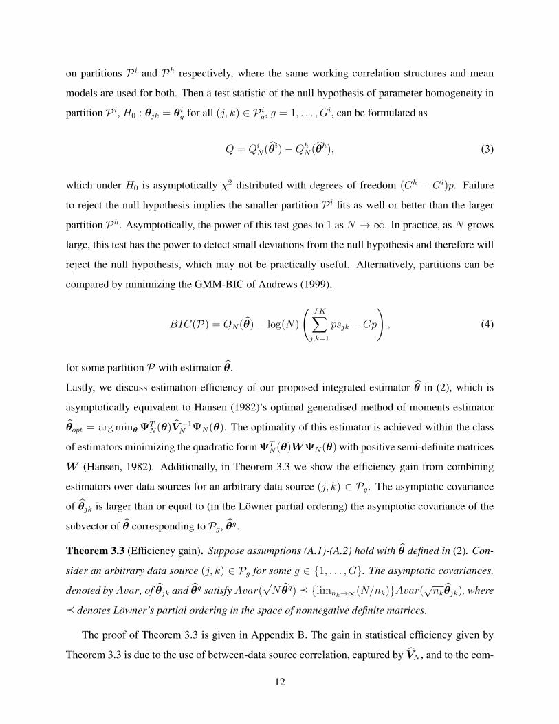
on partitions P i and Ph respectively, where the same working correlation structures and mean

models are used for both. Then a test statistic of the null hypothesis of parameter homogeneity in

partition P i, H0 : θjk = θig for all (j, k) ∈ P ig, g = 1, . . . , Gi, can be formulated as

Q = QiN(θi)−Qh

N(θh), (3)

which under H0 is asymptotically χ2 distributed with degrees of freedom (Gh − Gi)p. Failure

to reject the null hypothesis implies the smaller partition P i fits as well or better than the larger

partition Ph. Asymptotically, the power of this test goes to 1 as N →∞. In practice, as N grows

large, this test has the power to detect small deviations from the null hypothesis and therefore will

reject the null hypothesis, which may not be practically useful. Alternatively, partitions can be

compared by minimizing the GMM-BIC of Andrews (1999),

BIC(P) = QN(θ)− log(N)

(J,K∑j,k=1

psjk −Gp

), (4)

for some partition P with estimator θ.

Lastly, we discuss estimation efficiency of our proposed integrated estimator θ in (2), which is

asymptotically equivalent to Hansen (1982)’s optimal generalised method of moments estimator

θopt = arg minθ ΨTN(θ)V −1

N ΨN(θ). The optimality of this estimator is achieved within the class

of estimators minimizing the quadratic form ΨTN(θ)WΨN(θ) with positive semi-definite matrices

W (Hansen, 1982). Additionally, in Theorem 3.3 we show the efficiency gain from combining

estimators over data sources for an arbitrary data source (j, k) ∈ Pg. The asymptotic covariance

of θjk is larger than or equal to (in the Lowner partial ordering) the asymptotic covariance of the

subvector of θ corresponding to Pg, θg.

Theorem 3.3 (Efficiency gain). Suppose assumptions (A.1)-(A.2) hold with θ defined in (2). Con-

sider an arbitrary data source (j, k) ∈ Pg for some g ∈ {1, . . . , G}. The asymptotic covariances,

denoted byAvar, of θjk and θg satisfyAvar(√N θg) � {limnk→∞(N/nk)}Avar(

√nkθjk), where

� denotes Lowner’s partial ordering in the space of nonnegative definite matrices.

The proof of Theorem 3.3 is given in Appendix B. The gain in statistical efficiency given by

Theorem 3.3 is due to the use of between-data source correlation, captured by VN , and to the com-

12

bination of estimators within each Pg.

Finally, we remark that the proposed method is a generalization of Wang et al. (2012), which only

allows for combining over independent data sources. Here we introduce a non-diagonal weight ma-

trix VN to incorporate correlation between data sources, leading to improved statistical efficiency.

We also propose a closed form integrated estimator that is more computationally advantageous

than their iterative minimization procedure, leading to improved computational scalability.

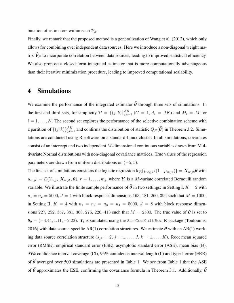
4 Simulations

We examine the performance of the integrated estimator θ through three sets of simulations. In

the first and third sets, for simplicity P = {(j, k)}J,Kj,k=1 (G = 1, d1 = JK) and Mi = M for

i = 1, . . . , N . The second set explores the performance of the selective combination scheme with

a partition of {(j, k)}J,Kj,k=1 and confirms the distribution of statistic QN(θ) in Theorem 3.2. Simu-

lations are conducted using R software on a standard Linux cluster. In all simulations, covariates

consist of an intercept and two independentM -dimensional continuous variables drawn from Mul-

tivariate Normal distributions with non-diagonal covariance matrices. True values of the regression

parameters are drawn from uniform distributions on (−5, 5).

The first set of simulations considers the logistic regression log{µir,jk/(1−µir,jk)} = Xir,jkθ with

µir,jk = E(Yir,jk|Xir,jk,θ), r = 1, . . . ,mj , where Yi is a M -variate correlated Bernoulli random

variable. We illustrate the finite sample performance of θ in two settings: in Setting I, K = 2 with

n1 = n2 = 5000, J = 4 with block response dimensions 163, 181, 260, 396 such that M = 1000;

in Setting II, K = 4 with n1 = n2 = n3 = n4 = 5000, J = 8 with block response dimen-

sions 227, 252, 357, 381, 368, 276, 226, 413 such that M = 2500. The true value of θ is set to

θ0 = (−4.44, 1.11,−2.22). Yi is simulated using the SimCorMultRes R package (Touloumis,

2016) with data source-specific AR(1) correlation structures. We estimate θ with an AR(1) work-

ing data source correlation structure (sjk = 2, j = 1, . . . , J , k = 1, . . . , K). Root mean squared

error (RMSE), empirical standard error (ESE), asymptotic standard error (ASE), mean bias (B),

95% confidence interval coverage (CI), 95% confidence interval length (L) and type-I error (ERR)

of θ averaged over 500 simulations are presented in Table 1. We see from Table 1 that the ASE

of θ approximates the ESE, confirming the covariance formula in Theorem 3.1. Additionally, θ

13

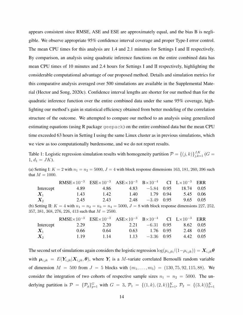
appears consistent since RMSE, ASE and ESE are approximately equal, and the bias B is negli-

gible. We observe appropriate 95% confidence interval coverage and proper Type-I error control.

The mean CPU times for this analysis are 1.4 and 2.1 minutes for Settings I and II respectively.

By comparison, an analysis using quadratic inference functions on the entire combined data has

mean CPU times of 10 minutes and 2.4 hours for Settings I and II respectively, highlighting the

considerable computational advantage of our proposed method. Details and simulation metrics for

this comparative analysis averaged over 500 simulations are available in the Supplemental Mate-

rial (Hector and Song, 2020c). Confidence interval lengths are shorter for our method than for the

quadratic inference function over the entire combined data under the same 95% coverage, high-

lighting our method’s gain in statistical efficiency obtained from better modeling of the correlation

structure of the outcome. We attempted to compare our method to an analysis using generalized

estimating equations (using R package geepack) on the entire combined data but the mean CPU

time exceeded 63 hours in Setting I using the same Linux cluster as in previous simulations, which

we view as too computationally burdensome, and we do not report results.

Table 1: Logistic regression simulation results with homogeneity partition P = {(j, k)}J,Kj,k=1 (G =1, d1 = JK).

(a) Setting I: K = 2 with n1 = n2 = 5000, J = 4 with block response dimensions 163, 181, 260, 396 suchthat M = 1000.

RMSE×10−3 ESE×10−3 ASE×10−3 B×10−4 CI L×10−3 ERRIntercept 4.89 4.86 4.83 −5.84 0.95 18.74 0.05X1 1.43 1.42 1.40 1.79 0.94 5.45 0.06X2 2.45 2.43 2.48 −3.49 0.95 9.65 0.05

(b) Setting II: K = 4 with n1 = n2 = n3 = n4 = 5000, J = 8 with block response dimensions 227, 252,357, 381, 368, 276, 226, 413 such that M = 2500.


The second set of simulations again considers the logistic regression log(µi,jk/(1−µi,jk)) = Xi,jkθ

with µi,jk = E(Yi,jk|Xi,jk,θ), where Yi is a M -variate correlated Bernoulli random variable

of dimension M = 500 from J = 5 blocks with (m1, . . . ,m5) = (130, 75, 92, 115, 88). We

consider the integration of two cohorts of respective sample sizes n1 = n2 = 5000. The un-

derlying partition is P = {Pg}Gg=1 with G = 3, P1 = {(1, k), (2, k)}Kk=1, P2 = {(3, k)}Kk=1

14

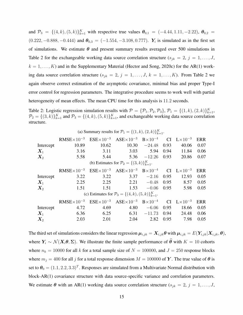
and P3 = {(4, k), (5, k)}Kk=1 with respective true values θ0,1 = (−4.44, 1.11,−2.22), θ0,2 =

(0.222,−0.888,−0.444) and θ0,3 = (−1.554,−3.108, 0.777). Yi is simulated as in the first set

of simulations. We estimate θ and present summary results averaged over 500 simulations in

Table 2 for the exchangeable working data source correlation structure (sjk = 2, j = 1, . . . , J ,

k = 1, . . . , K) and in the Supplementary Material (Hector and Song, 2020c) for the AR(1) work-

ing data source correlation structure (sjk = 2, j = 1, . . . , J , k = 1, . . . , K). From Table 2 we

again observe correct estimation of the asymptotic covariance, minimal bias and proper Type-I

error control for regression parameters. The integrative procedure seems to work well with partial

heterogeneity of mean effects. The mean CPU time for this analysis is 11.2 seconds.

Table 2: Logistic regression simulation results with P = {P1,P2,P3}, P1 = {(1, k), (2, k)}Kk=1,P2 = {(3, k)}Kk=1 and P3 = {(4, k), (5, k)}Kk=1, and exchangeable working data source correlationstructure.

(a) Summary results for P1 = {(1, k), (2, k)}Kk=1.


(b) Estimates for P2 = {(3, k)}Kk=1.

RMSE×10−3 ESE×10−3 ASE×10−3 B×10−4 CI L×10−3 ERRIntercept 3.22 3.22 3.37 −2.16 0.95 12.93 0.05X1 2.25 2.25 2.21 −0.48 0.95 8.57 0.05X2 1.51 1.51 1.53 −0.06 0.95 5.98 0.05

(c) Estimates for P3 = {(4, k), (5, k)}Kk=1.

RMSE×10−3 ESE×10−3 ASE×10−3 B×10−4 CI L×10−3 ERRIntercept 4.72 4.69 4.80 −6.06 0.95 18.66 0.05X1 6.36 6.25 6.31 −11.73 0.94 24.48 0.06X2 2.03 2.01 2.04 2.82 0.95 7.98 0.05

The third set of simulations considers the linear regressionµi,jk = Xi,jkθ withµi,jk = E(Yi,jk|Xi,jk,θ),

where Yi ∼ N (Xiθ,Σ). We illustrate the finite sample performance of θ with K = 10 cohorts

where nk = 10000 for all k for a total sample size of N = 100000, and J = 250 response blocks

where mj = 400 for all j for a total response dimension M = 100000 of Y . The true value of θ is

set to θ0 = (1.1, 2.2, 3.3)T . Responses are simulated from a Multivariate Normal distribution with

block-AR(1) covariance structure with data source-specific variance and correlation parameters.

We estimate θ with an AR(1) working data source correlation structure (sjk = 2, j = 1, . . . , J ,

15

k = 1, . . . , K). RMSE, ESE, ASE, B, CI, L and ERR of θ averaged over 500 simulations are

presented in Table 3. We observe in Table 3 slight inflation of Type-I error due to under-estimation

of the asymptotic covariance. This is potentially due to the high-dimensionality of ΨN and VN ,

which have dimension 15000, leading to numerical instability. This under-estimation is similar to

the generalised method of moments case and is discussed in Section 6. The performance of our

method in this ultra-high dimension is nonetheless remarkable: with 1010 data points with high-

variability in both outcomes and covariates, the procedure is able to estimate and infer the true

mean effects with minimal bias and only slight under-coverage. The mean CPU time for this anal-

ysis is 17.9 hours.

Table 3: Linear regression simulation results with homogeneity partitionP = {(j, k)}J,Kj,k=1 (G = 1,d1 = JK).

RMSE×10−4 ESE×10−4 ASE×10−4 B×10−6 CI L×10−4 ERRIntercept 2.26 2.25 1.99 −21.03 0.93 7.81 0.07X1 0.35 0.35 0.31 −0.15 0.92 1.22 0.08X2 0.35 0.35 0.31 1.07 0.93 1.22 0.07

In the Supplementary Material (Hector and Song, 2020c), a quantile-quantile plot of the chi-

squared statistic from Theorem 3.2 in the second set of simulations illustrates its appropriate

asymptotic distribution. A quantile-quantile plot of the Q statistic in (3) in the linear regression

setting comparing two partitions, one integrating over cohort only and one integrating over all data

sources, is also given in the Supplementary Material (Hector and Song, 2020c).

5 METSIM analysis

We illustrate the application of the proposed method to the integrative analysis of metabolic path-

ways in the METSIM study described in Section 2. The METSIM study profiled N = 6223 men

in K = 4 separate samples with sample sizes n1 = 1229, n2 = 2950, n3 = 1045 and n4 = 999.

They measured 1018 metabolites belonging to 112 sub-pathways grouped in eight pathways with

distinct biological functions. For each pathway, we investigate the association between smoking

and metabolites in the pathway using our distributed and integrated quadratic inference functions

approach to account for heterogeneity and correlation in metabolite sub-pathways.

Consider pathway s ∈ {1, . . . , 8}. To illustrate the statistical efficiency gains from accounting

16

for correlation between sub-pathways and combining models over independent cohorts, we first

estimate sub-pathway and cohort specific effects and integrate them over cohorts (but not over

sub-pathways); we then selectively combine regression models across sub-pathways based on a

known partition P . More specifically, we first estimate a heterogeneous model with partition

Ph = {Phj }Jj=1, Phj = {(j, 1), . . . , (j,K)} that yields unique values of the regression coefficients

for each sub-pathway. We then create a partition P i of Ph with cardinality G by selectively com-

bining sub-pathways based on prior knowledge and estimate an integrative model. Details on the

combination scheme can be found in the Supplementary Material (Hector and Song, 2020c) along

with plots of parameters estimates. Note that the energy pathway is only constituted of two sub-

pathways which cannot be combined.

We describe the marginal model for metabolites in pathway s. Denote by J the number of sub-

pathways and M the number of metabolites in pathway s. Let yir,jk denote the value of metabo-

lite r ∈ {1, . . . ,mj} in sub-pathway j ∈ {1, . . . , J} for participant i ∈ {1, . . . , nk} in cohort

k ∈ {1, . . . , K}, and let yjk = (yir,jk)nk,mj

i,r=1 . Consider the marginal regression model

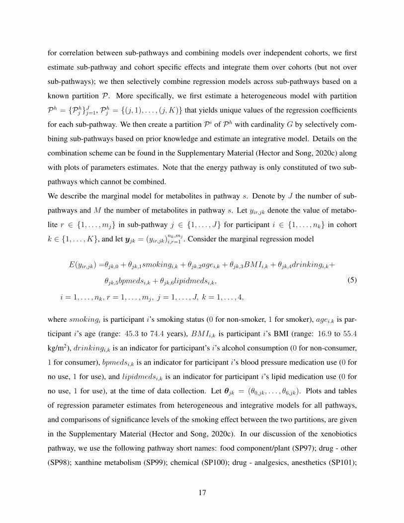
E(yir,jk) =θjk,0 + θjk,1smokingi,k + θjk,2agei,k + θjk,3BMIi,k + θjk,4drinkingi,k+

θjk,5bpmedsi,k + θjk,6lipidmedsi,k,

i = 1, . . . , nk, r = 1, . . . ,mj, j = 1, . . . , J, k = 1, . . . , 4,

(5)

where smokingi is participant i’s smoking status (0 for non-smoker, 1 for smoker), agei.k is par-

ticipant i’s age (range: 45.3 to 74.4 years), BMIi,k is participant i’s BMI (range: 16.9 to 55.4

kg/m2), drinkingi,k is an indicator for participant’s i’s alcohol consumption (0 for non-consumer,

1 for consumer), bpmedsi,k is an indicator for participant i’s blood pressure medication use (0 for

no use, 1 for use), and lipidmedsi,k is an indicator for participant i’s lipid medication use (0 for

no use, 1 for use), at the time of data collection. Let θjk = (θ0,jk, . . . , θ6,jk). Plots and tables

of regression parameter estimates from heterogeneous and integrative models for all pathways,

and comparisons of significance levels of the smoking effect between the two partitions, are given

in the Supplementary Material (Hector and Song, 2020c). In our discussion of the xenobiotics

pathway, we use the following pathway short names: food component/plant (SP97); drug - other

(SP98); xanthine metabolism (SP99); chemical (SP100); drug - analgesics, anesthetics (SP101);

17

benzoate metabolism (SP102); tobacco Metabolite (SP103); drug - topical agents (SP104); drug -

antibiotic (SP105); drug - cardiovascular (SP106); drug - neurological (SP107); drug - respiratory

(SP108); drug - psychoactive (SP109); drug - gastrointestinal (SP110); bacterial/fungal (SP111);

drug - metabolic (SP112).

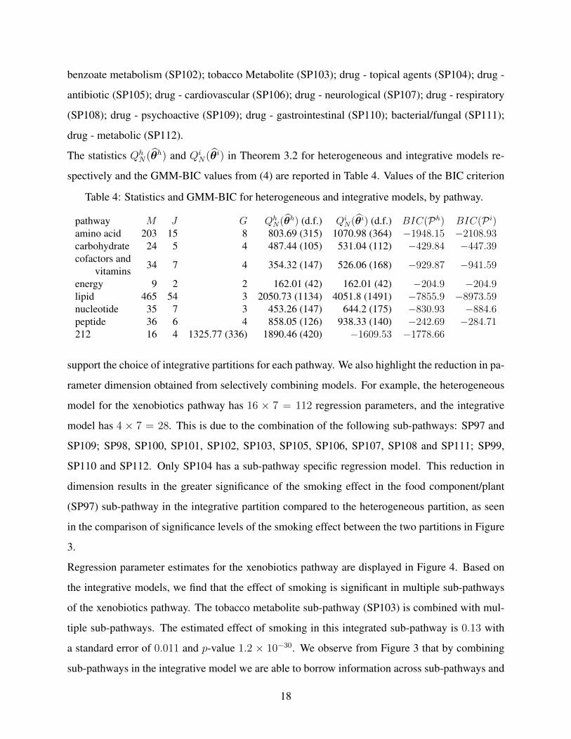
The statistics QhN(θh) and Qi

N(θi) in Theorem 3.2 for heterogeneous and integrative models re-

spectively and the GMM-BIC values from (4) are reported in Table 4. Values of the BIC criterion

Table 4: Statistics and GMM-BIC for heterogeneous and integrative models, by pathway.

pathway M J G QhN(θh) (d.f.) Qi

N(θi) (d.f.) BIC(Ph) BIC(P i)amino acid 203 15 8 803.69 (315) 1070.98 (364) −1948.15 −2108.93carbohydrate 24 5 4 487.44 (105) 531.04 (112) −429.84 −447.39cofactors and

34 7 4 354.32 (147) 526.06 (168) −929.87 −941.59vitamins

energy 9 2 2 162.01 (42) 162.01 (42) −204.9 −204.9lipid 465 54 3 2050.73 (1134) 4051.8 (1491) −7855.9 −8973.59nucleotide 35 7 3 453.26 (147) 644.2 (175) −830.93 −884.6peptide 36 6 4 858.05 (126) 938.33 (140) −242.69 −284.71212 16 4 1325.77 (336) 1890.46 (420) −1609.53 −1778.66

support the choice of integrative partitions for each pathway. We also highlight the reduction in pa-

rameter dimension obtained from selectively combining models. For example, the heterogeneous

model for the xenobiotics pathway has 16 × 7 = 112 regression parameters, and the integrative

model has 4 × 7 = 28. This is due to the combination of the following sub-pathways: SP97 and

SP109; SP98, SP100, SP101, SP102, SP103, SP105, SP106, SP107, SP108 and SP111; SP99,

SP110 and SP112. Only SP104 has a sub-pathway specific regression model. This reduction in

dimension results in the greater significance of the smoking effect in the food component/plant

(SP97) sub-pathway in the integrative partition compared to the heterogeneous partition, as seen

in the comparison of significance levels of the smoking effect between the two partitions in Figure

3.

Regression parameter estimates for the xenobiotics pathway are displayed in Figure 4. Based on

the integrative models, we find that the effect of smoking is significant in multiple sub-pathways

of the xenobiotics pathway. The tobacco metabolite sub-pathway (SP103) is combined with mul-

tiple sub-pathways. The estimated effect of smoking in this integrated sub-pathway is 0.13 with

a standard error of 0.011 and p-value 1.2 × 10−30. We observe from Figure 3 that by combining

sub-pathways in the integrative model we are able to borrow information across sub-pathways and

18

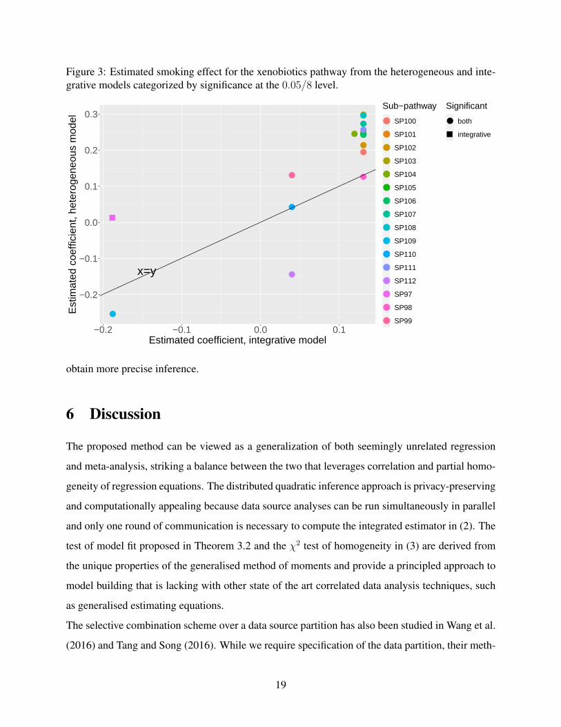
Figure 3: Estimated smoking effect for the xenobiotics pathway from the heterogeneous and inte-grative models categorized by significance at the 0.05/8 level.

●

●

●

●

● ●●

●●

●

●

●

●

●●

x=y

−0.2

−0.1

0.0

0.1

0.2

0.3

−0.2 −0.1 0.0 0.1Estimated coefficient, integrative model

Est

imat

ed c

oeffi

cien

t, he

tero

gene

ous

mod

el

Sub−pathway

●

●

●

●

●

●

●

●

●

●

●

●

●

●

●

●

SP100

SP101

SP102

SP103

SP104

SP105

SP106

SP107

SP108

SP109

SP110

SP111

SP112

SP97

SP98

SP99

Significant

● both

integrative

obtain more precise inference.

6 Discussion

The proposed method can be viewed as a generalization of both seemingly unrelated regression

and meta-analysis, striking a balance between the two that leverages correlation and partial homo-

geneity of regression equations. The distributed quadratic inference approach is privacy-preserving

and computationally appealing because data source analyses can be run simultaneously in parallel

and only one round of communication is necessary to compute the integrated estimator in (2). The

test of model fit proposed in Theorem 3.2 and the χ2 test of homogeneity in (3) are derived from

the unique properties of the generalised method of moments and provide a principled approach to

model building that is lacking with other state of the art correlated data analysis techniques, such

as generalised estimating equations.

The selective combination scheme over a data source partition has also been studied in Wang et al.

(2016) and Tang and Song (2016). While we require specification of the data partition, their meth-

19

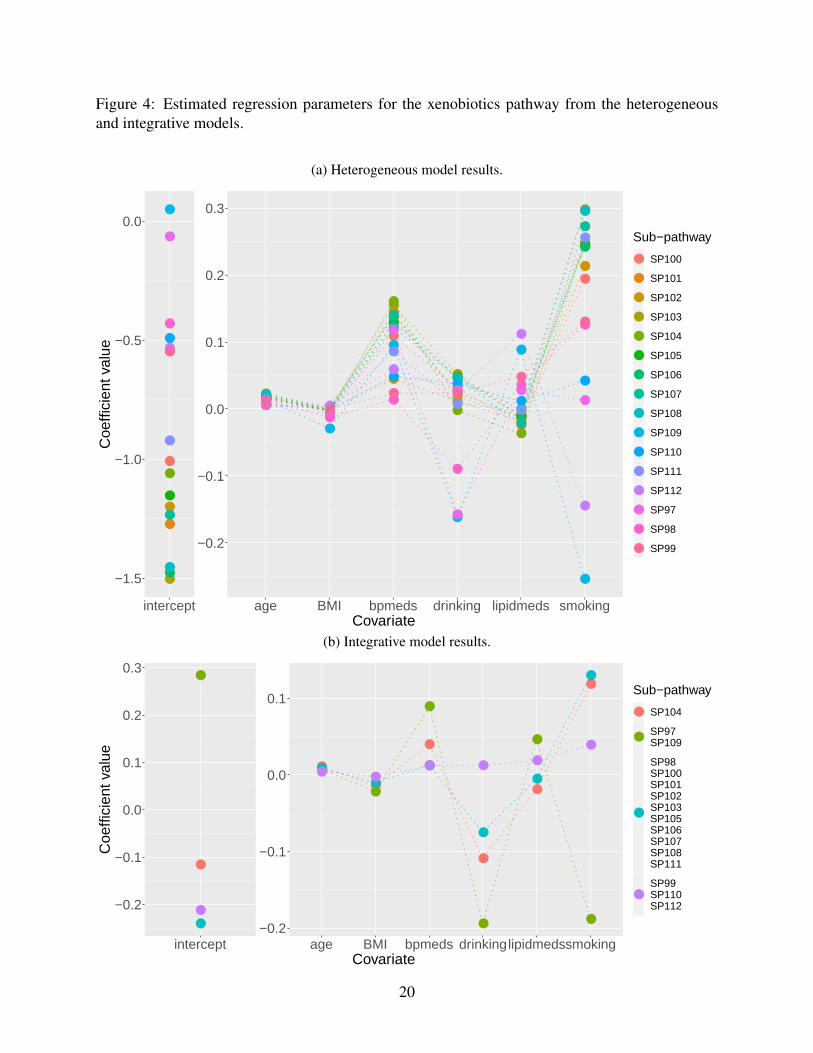
Figure 4: Estimated regression parameters for the xenobiotics pathway from the heterogeneousand integrative models.

(a) Heterogeneous model results.

●

●

●

●

●

●

●

●

●

●

●

●

●

●

●

●

●●

●

●

●

●

●

●

●

●

●

●

●

●●

●

●

●

●

●

●

●

●

●

●

● ●

●

●

●

●●

●

●

●

●

●●

●

●

●

●

●●

●

●

●

●

●

●

●

●

●

●

●

●

●

● ●

●

● ●

●●

●

●

●●

●

●

●

●

● ●

●

●

●

●

●●

●

●

●●●

●

●

●

●

●

● ●

●●

●

●

intercept age BMI bpmeds drinking lipidmeds smoking

−0.2

−0.1

0.0

0.1

0.2

0.3

−1.5

−1.0

−0.5

0.0

Covariate

Coe

ffici

ent v

alue

Sub−pathway

●

●

●

●

●

●

●

●

●

●

●

●

●

●

●

●

SP100

SP101

SP102

SP103

SP104

SP105

SP106

SP107

SP108

SP109

SP110

SP111

SP112

SP97

SP98

SP99

(b) Integrative model results.

●

●

●●

●

●

●

●

●

●

●

●

●

●

●

●

●

●

●

●●

●

● ●●● ●

●

intercept age BMI bpmeds drinkinglipidmedssmoking−0.2

−0.1

0.0

0.1

−0.2

−0.1

0.0

0.1

0.2

0.3

Covariate

Coe

ffici

ent v

alue

Sub−pathway

●

●

●

●

SP104

SP97SP109

SP98SP100SP101SP102SP103SP105SP106SP107SP108SP111

SP99SP110SP112

20

ods learn the partition in a data-driven way, which can be advantageous. Inference with the fused

lasso, however, is burdened by debiasing methods that can be ill-defined or computationally bur-

densome. Additionally, the fused lasso approaches do not provide a formal procedure to test the

validity of the parameter fusion scheme, relying instead on visualization such as dendograms. Our

method is clearly advantageous when an approximately known partition exists.

Limitations of the proposed method include the need for a pre-defined partition of data sources

defining regions of parameter homogeneity, which typically is given by related scientific knowl-

edge but may occasionally be lacking in practice. Data pre-processing and learning and the test

in (3) may help in determining an appropriate partition. Additionally, standard errors tend to be

underestimated in small sample sizes or when the dimension of the moment conditions is large;

this phenomenon has been well documented in the generalised method of moments (see Hansen

et al. (1996) and others in the same issue).

Acknowledgements

We are very grateful to Drs. Michael Boehnke and Markku Laakso for their generosity in let-

ting us use their data. We are grateful to Dr. Lan Luo for sharing her code to estimate parame-

ters using quadratic inference functions. This work was supported by grants R01ES024732 and

NSF1811734.

A Assumptions

(A.1) Assumptions for consistency and asymptotic normality of θjk for data source (j, k) in gth

partition set Pg:

(i) C−1jk is positive definite and C−1

jk Eθ0,g{ψi,jk(θjk)} = 0 if and only if θjk = θ0,g

(ii) the true value θ0 = (θ0,g)Gg=1 is an interior point of Θ = ×Gg=1Θg, and Θg are compact

(iii) ψi,jk(θjk) is continuous at each θjk with probability one

(iv) Eθ0{supθjk∈Θg‖ψi,jk(θjk)‖} <∞

21

(v) ψi,jk(θjk) is continuously differentiable in a neighborhood N of θ0,g with probability

approaching one

(vi) Eθ0,g{ψi,jk(θ0,g)} = 0 and Eθ0,g{‖ψi,jk(θ0,g)‖2} is finite and positive-definite

(vii) Eθ0{supθjk∈N∥∥∇θjkψi,jk(θjk)

∥∥} <∞; [Eθ0{∇θ0,gψi,jk(θ0,g)}]TC−1jk Eθ0{∇θ0,gψi,jk(θ0,g)}

is nonsingular

(A.2) For any δN → 0,

sup‖θ−θ0‖≤δN

N1/2

1 +N1/2 ‖θ − θ0‖‖ΨN(θ)−ΨN(θ0)− Eθ0ΨN(θ)‖ = Op(N

−1/2).

B Proof of Theorem 3.3

Let vjk(θjk) = V arθ0,g(ψi,jk(θjk)) . From assumption (A.1) and Theorem 3.1, Avar(√nkθjk) =

{sjk(θ0,g)v−1jk (θ0,g)s

Tjk(θ0,g)}−1, and

Avar(√N θ) =

{sT (θ0)v−1(θ0)s(θ0)

}−1, Avar(

√N θg) =

[{sT (θ0)v−1(θ0)s(θ0)

}−1]g,

where [A]g denotes the submatrix of a matrixA consisting of rows and columns corresponding to

data sources in Pg. Let [v(θ)](j,k) denote submatrix of v(θ) consisting of rows and columns cor-

responding to data source (j, k), and let [v(θ)]−(j,k);, [v(θ)];−(j,k) and [v(θ)]−(j,k) denote the sub-

matrices of v(θ) eliminating respectively rows, columns, and rows and columns corresponding to

data source (j, k). Clearly (nk/N)vjk(θjk) is a submatrix of v(θ): (nk/N)vjk(θjk) = [v(θ)](j,k).

Consider (j, k) = (1, 1), which is in partition setPg1 for some g1 ∈ {1, . . . , G} (this is without loss

of generality since we can reorganize the rows of ψi for (j, k) 6= (1, 1) to make (j, k) = (1, 1)).

We write

v(θ) =

[v(θ)](1,1) [v(θ)];−(1,1)

[v(θ)]−(1,1); [v(θ)]−(1,1)

.

22

By Corollary 7.7.4. in Horn and Johnson (1990),

s11(θg0,1)v−111 (θg0,1)sT11(θg0,1) ≺ s11(θg0,1)

n1

N

[v−1(θ0)

](1,1)

sT11(θg0,1)

where � denotes Lowner’s partial ordering in the space of nonnegative definite matrices. By the

definition of sg1(θg0,1) in Section 3.4, this implies that

{sTg1(θg0,1)

[v−1(θ0)

]g1sg1(θg0,1)

}−1

≺{n1

Ns11(θg0,1)v−1

11 (θg0,1)sT11(θg0,1)}−1

= limn1→∞

N

n1

Avar(√n1θ11).

Again by Corollary 7.7.4. in Horn and Johnson (1990), we have that

Avar(√N θg1) =

[{sT (θ0)v−1(θ0)s(θ0)

}−1]g1≺{sTg1(θg0,1)

[v−1(θ0)

]g1sg1(θg0,1)

}−1

,

implying Avar(√N θg1) � {limnk→∞(N/nk)}Avar(

√n1θ11).

References

Andrews, D. W. (1999). Consistent moment selection procedures for generalized method of mo-

ments estimation. Econometrica, 67(3):543–564.

Caragea, P. and Smith, R. L. (2007). Asymptotic properties of computationally efficient alter-

native estimators for a class of multivariate normal models. Journal of Multivariate Analysis,

98(7):1417–1440.

Cho, H. and Qu, A. (2015). Efficient estimation for longitudinal data by combining large-

dimensional moment conditions. Electronic Journal of Statistics, 9:1315–1334.

Claggett, B., Xie, M., and Tian, L. (2014). Meta-analysis with fixed, unknown, study-specific

parameters. Journal of the American Statistical Association, 109(508):1660–1671.

DerSimonian, R. and Laird, N. (2015). Meta-analysis in clinical trials revisited. Contemporary

Clinical Trials, 45:139–145.

23

Fan, J., Han, F., and Liu, H. (2014). Challenges of big data analysis. National Science Review,

1(2):293–314.

Glass, G. V. (1976). Primary, secondary, and meta-analysis of research. Educational Researcher,

5(10):3–8.

Godambe, V. P. and Heyde, C. C. (1987). Quasi-likelihood and optimal estimation. International

Statistical Review, 55(3):231–244.

Hansen, L. P. (1982). Large sample properties of generalized method of moments estimators.

Econometrica, 50(4):1029–1054.

Hansen, L. P., Heaton, J., and Yaron, A. (1996). Finite-sample properties of some alternative GMM

estimators. Journal of Business and Economic Statistics, 14(3):262–280.

Hector, E. C. and Song, P. X.-K. (2020a). A distributed and integrated method of moments for

high-dimensional correlated data analysis. Journal of the American Statistical Association, DOI:

10.1080/01621459.2020.1736082:1–14.

Hector, E. C. and Song, P. X.-K. (2020b). Doubly distributed supervised learning and inference

with high-dimensional correlated outcomes. Journal of Machine Learning Research, 21:1–35.

Hector, E. C. and Song, P. X.-K. (2020c). Supplement to “Joint integrative analysis of multiple

data sources with correlated vector outcomes”. Available upon request.

Horn, R. A. and Johnson, C. R. (1990). Matrix analysis. New York: Cambridge University Press.

Hu, Y. and Song, P. X.-K. (2012). Sample size determination for quadratic inference functions in

longitudinal design with dichotomous outcomes. Statistics in Medicine, 31(8):787–800.

Ioannidis, J. P. (2006). Meta-analysis in public health: potentials and problems. Italian Journal of

Public Health, 3(2):9–14.

Jordan, M. I. (2013). On statistics, computation and scalability. Bernoulli, 19(4):1378–1390.

Kundu, P., Tang, R., and Chatterjee, N. (2019). Generalized meta-analysis for multiple regression

models across studies with disparate covariate information. Biometrika, 106(3):567–585.

24

Laakso, M., Kuusisto, J., Stancakova, A., Kuulasmaa, T., Pajukanta, P., Lusis, A. J., Collins, F. S.,

Mohlke, K. L., and Boehnke, M. (2017). The Metabolic Syndrome in Men study: a resource for

studies of metabolic and cardiovascular diseases. Journal of Lipid Research, 58(3):481–493.

Lin, D.-Y. and Zeng, D. (2010). On the relative efficiency of using summary statistics versus

individual-level data in meta-analysis. Biometrika, 97(2):321–332.

Liu, D., Liu, R. Y., and Xie, M. (2015). Multivariate meta-analysis of heterogeneous studies

using only summary statistics: efficiency and robustness. Journal of the American Statistical

Association, 110(509):326–340.

Qu, A., Lindsay, B. G., and Li, B. (2000). Improving generalised estimating equations using

quadratic inference functions. Biometrika, 87(4):823–836.

Smith, T. C., Spiegelhalter, D. J., and Thomas, A. (1995). Bayesian approaches to random-effects

meta-analysis: a comparative study. Statistics in Medicine, 14(24):2685–2699.

Song, P. X.-K. (2007). Correlated Data Analysis: Modeling, Analytics, and Applications. Springer

Series in Statistics.

Tang, L. and Song, P. X.-K. (2016). Fused lasso approach in regression coefficients clustering –

learning parameter heterogeneity in data integration. Journal of Machine Learning Research,

17:1–23.

Touloumis, A. (2016). Simulating correlated binary and multinomial responses under marginal

model specification: The simcormultres package. The R Journal, 8(2):79–91.

Varin, C. (2008). On composite marginal likelihoods. Advances in Statistical Analysis, 92(1):1–28.

Wang, F., Wang, L., and Song, P. X. K. (2012). Quadratic inference function approach to merging

longitudinal studies: validation and joint estimation. Biometrika, 99(3):755–762.

Wang, F., Wang, L., and Song, P. X.-K. (2016). Fused lasso with the adaptation of parameter

ordering in combining multiple studies with repeated measurements. Biometrics, 72(4):1184–

1193.

25

Xie, M. and Singh, K. (2013). Confidence distribution, the frequentist distribution estimator of a

parameter: a review. International Statistical Review, 81(1):3–39.

Xie, M., Singh, K., and Strawderman, W. E. (2011). Confidence distributions and a unifying

framework for meta-analysis. Journal of the American Statistical Association, 106(493):320–

333.

Yang, G., Liu, D., Liu, R. Y., Xie, M., and Hoaglin, D. C. (2014). Efficient network meta-analysis:

a confidence distribution approach. Statistical Methodology, 20:105–125.

Zellner, A. (1962). An efficient method of estimating seemingly unrelated regressions and tests for

aggregation bias. Journal of the American Statistical Association, 57(298):348–368.

26

Documents

Joint integrative analysis of multiple data sources with