1

Joint Inference of Multiple Label Types in Large Networks

Deepayan Chakrabarti (deepay@fb.com)

Stanislav Funiak(sfuniak@fb.com

)

Jonathan Chang(jonchang@fb.com

)

Sofus A. Macskassy (sofmac@fb.com)

2

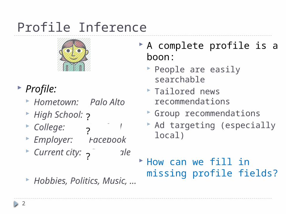
Profile Inference

Profile: Hometown: Palo Alto High School: Gunn College: Stanford Employer: Facebook Current city:

Sunnyvale

Hobbies, Politics, Music, …

A complete profile is a boon: People are easily

searchable Tailored news

recommendations Group recommendations Ad targeting (especially

local)

How can we fill in missing profile fields?

?

?

?

3

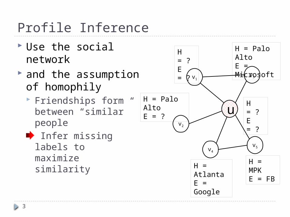
Profile Inference Use the social

network and the assumption

of homophily Friendships form

between “similar” people Infer missing labels to maximize similarity

u

v1

v2

v3

v4v5

H = Palo AltoE = Microsoft

H = MPKE = FB

H = AtlantaE = Google

H = Palo AltoE = ?

H = ?E = ?

H = ?E = ?

4

Previous Work Random walks [Talukdar+/09, Baluja+/08] Statistical Relational Learning [Lu+/03,

Macskassy+/07] Relational Dependency Networks

[Neville+/07] Latent models [Palla+/12]

Either: too generic; require too much labeled data; do not handle multiple label types; are outperformed by label propagation

[Macskassy+/07]

5

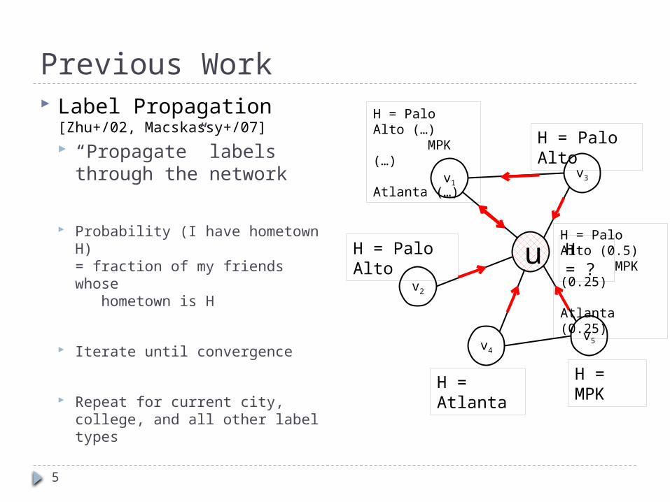
Previous Work Label Propagation

[Zhu+/02, Macskassy+/07]

“Propagate” labels through the network

Probability (I have hometown H)= fraction of my friends whose hometown is H

Iterate until convergence

Repeat for current city, college, and all other label types

u

v1

v2

v3

v4v5

H = Palo Alto

H = MPK

H = Atlanta

H = Palo Alto

H = ?

H = Palo Alto (0.5) MPK (0.25) Atlanta (0.25)

H = Palo Alto (…) MPK (…) Atlanta (…)

6

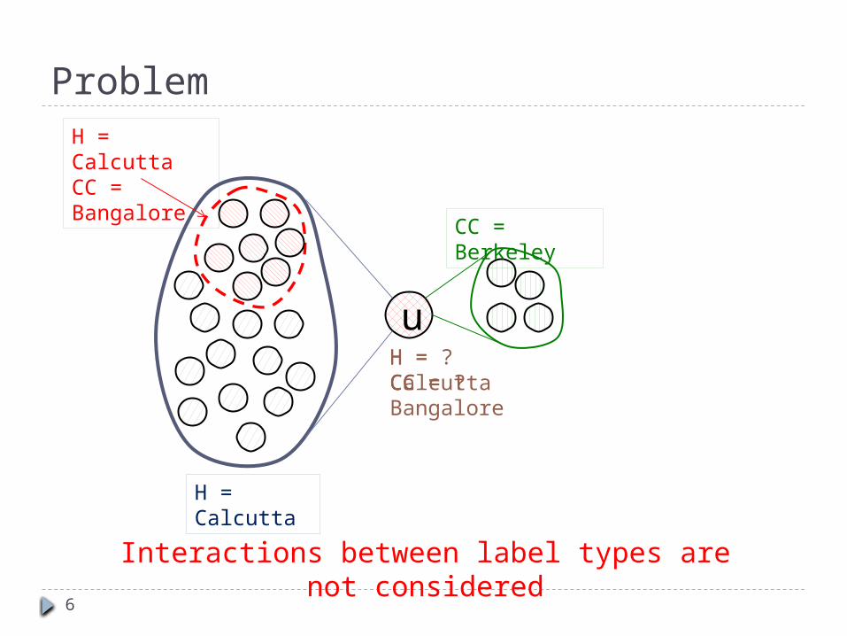
Problem

u

H = Calcutta

H = CalcuttaCC = Bangalore

CC = Berkeley

H = ?CC = ?H = CalcuttaCC = Bangalore

Interactions between label types are not considered

7

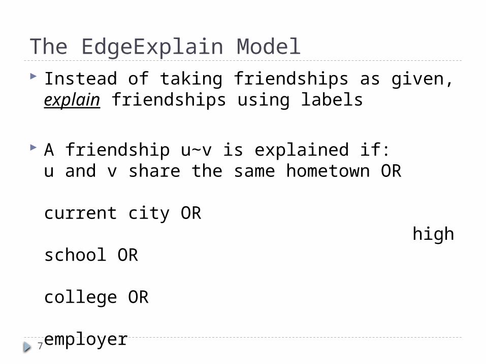
The EdgeExplain Model Instead of taking friendships as given,

explain friendships using labels

A friendship u∼v is explained if:u and v share the same hometown OR current city OR high school OR college OR employer

8

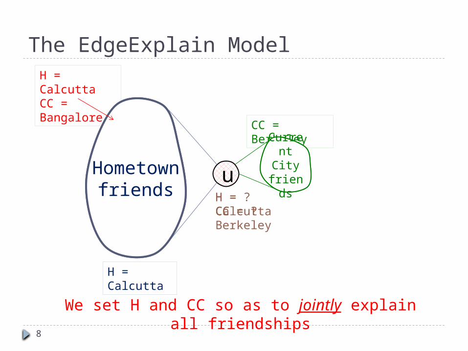
The EdgeExplain Model

u

H = Calcutta

H = CalcuttaCC = Bangalore

CC = Berkeley

H = ?CC = ?H = CalcuttaCC = Berkeley

Hometown friends

Current City

friends

We set H and CC so as to jointly explain all friendships

9

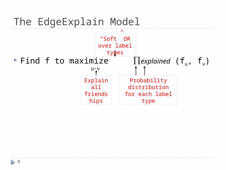
Find f to maximize ∏explained (fu, fv)The EdgeExplain Model

u∼v

“Soft” ORover label

types

Probability distribution for each label type

Explain all

friendships

10

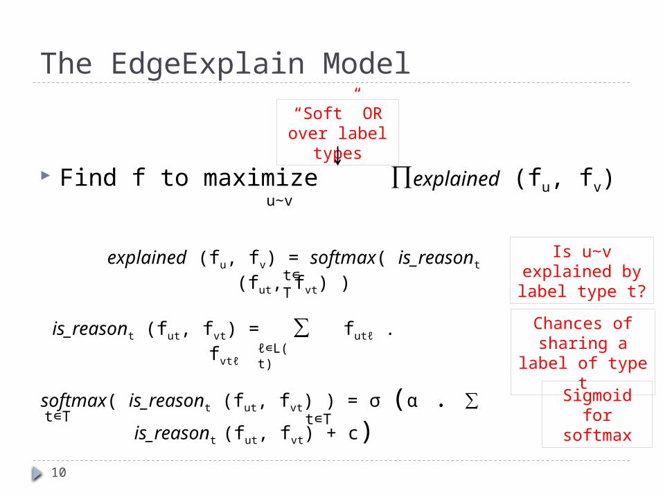
Find f to maximize ∏explained (fu, fv)The EdgeExplain Model

u∼v

“Soft” ORover label

types

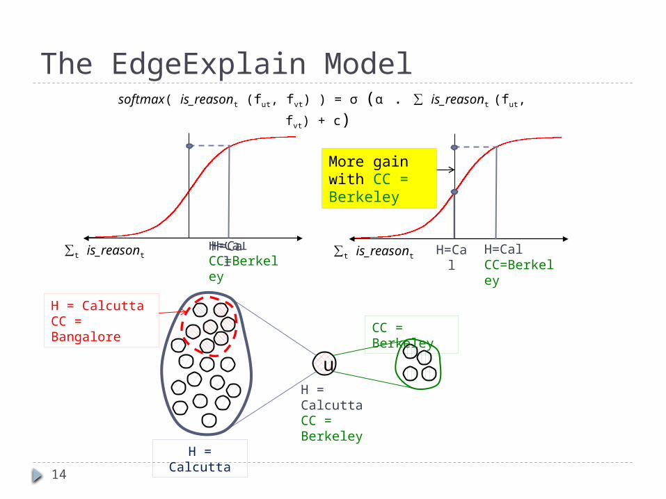
explained (fu, fv) = softmax( is_reasont (fut, fvt) )t∊Τis_reasont (fut, fvt) = ∑ futℓ . fvtℓℓ∊L(t)softmax( is_reasont (fut, fvt) ) = σ (α . ∑ is_reasont (fut, fvt) + c) t∊Τ t∊Τ

Is u∼v explained by label type t?

Chances of sharing a label

of type t

Sigmoid for softmax

11

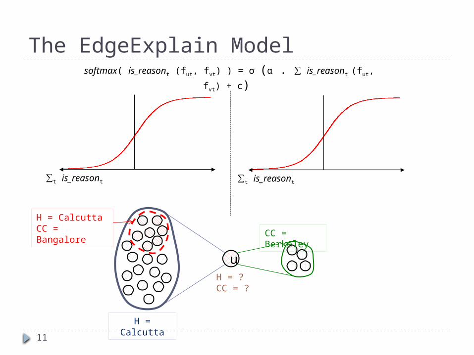
H = ?CC = ?

The EdgeExplain Model

∑t is_reasont

u

H = Calcutta

CC = Berkeley

H = CalcuttaCC = Bangalore

∑t is_reasont

softmax( is_reasont (fut, fvt) ) = σ (α . ∑ is_reasont (fut, fvt) + c)

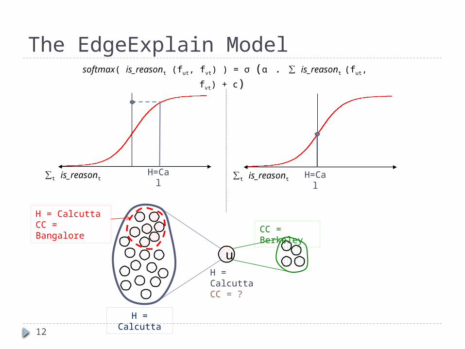
12

The EdgeExplain Model

H = CalcuttaCC = ?

∑t is_reasont

u

H = Calcutta

CC = Berkeley

H = CalcuttaCC = Bangalore

∑t is_reasontH=Cal H=Cal

softmax( is_reasont (fut, fvt) ) = σ (α . ∑ is_reasont (fut, fvt) + c)

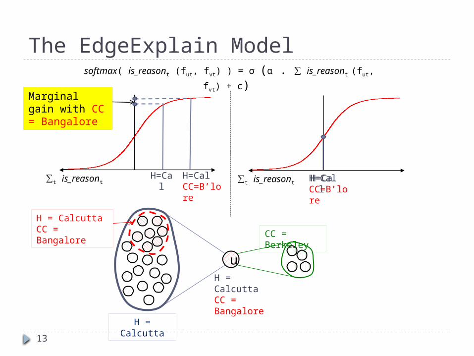
13

H = CalcuttaCC = Bangalore

The EdgeExplain Model

∑t is_reasont H=Cal

Marginal gain with CC = Bangalore

u

H = Calcutta

CC = Berkeley

H = CalcuttaCC = Bangalore

∑t is_reasont H=CalH=CalCC=B’lore H=CalCC=B’lore

softmax( is_reasont (fut, fvt) ) = σ (α . ∑ is_reasont (fut, fvt) + c)

14

H=CalCC=Berkeley

H = CalcuttaCC = Berkeley

The EdgeExplain Model

∑t is_reasont H=Cal

u

H = Calcutta

CC = Berkeley

H = CalcuttaCC = Bangalore

∑t is_reasont H=Cal H=CalCC=Berkeley

More gain with CC = Berkeley

softmax( is_reasont (fut, fvt) ) = σ (α . ∑ is_reasont (fut, fvt) + c)

15

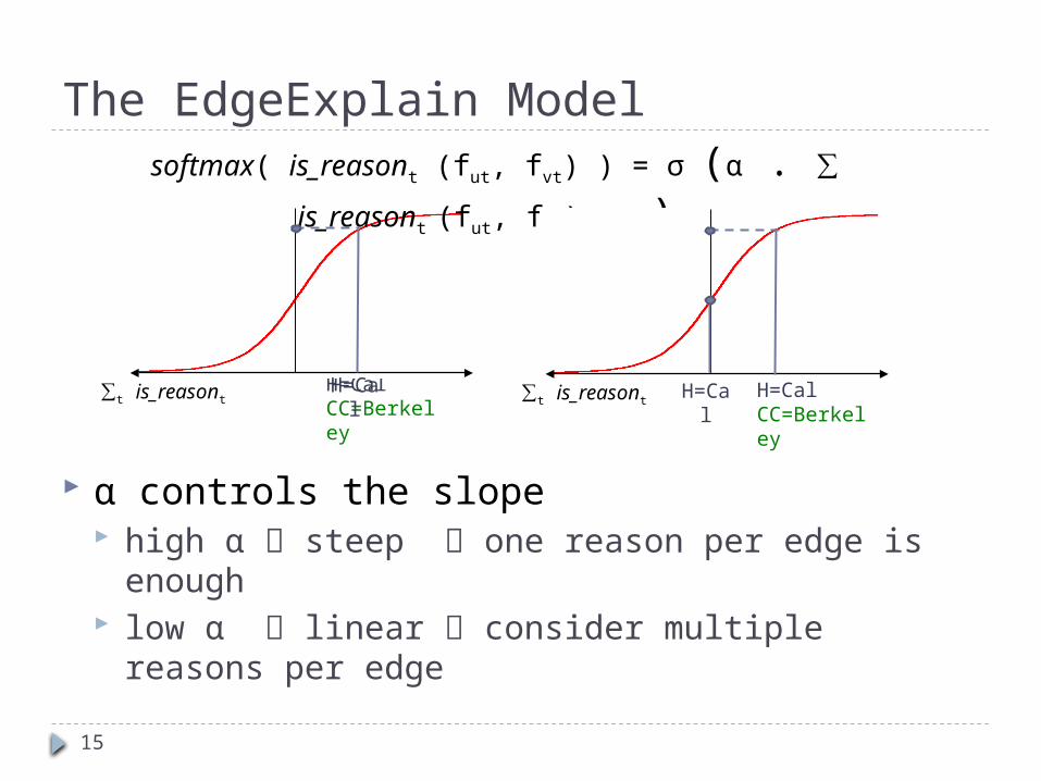
α controls the slope high α steep one reason per edge is enough low α linear consider multiple reasons per edge

H=CalCC=Berkeley

The EdgeExplain Modelsoftmax( is_reasont (fut, fvt) ) = σ (α . ∑ is_reasont (fut, fvt) + c)

∑t is_reasont H=Cal ∑t is_reasont H=Cal H=CalCC=Berkeley

16

Experiments 1.1B users of the Facebook social network O(10M) labels 5-fold cross-validation Measure recall

Did we get the correct label in our top prediction? Top-3?

Inference: proximal gradient descent implemented via message-passing in Apache Giraph

[Ching/13]

Sparsify graph by considering K closest friends by age

17

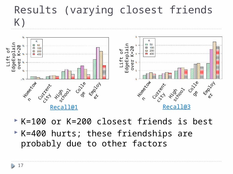
Results (varying closest friends K)

K=100 or K=200 closest friends is best K=400 hurts; these friendships are probably

due to other factors

Recall@1 Recall@3Hom

eto

wn Cu

rren

t ci

ty Hig

h sc

hool Co

llege Em

ploy

er

Lift

of

Ed

geExpla

in o

ver

K=

20

Lift

of

Ed

geExpla

in o

ver

K=

20

Hom

eto

wn Cu

rren

t ci

ty Hig

h sc

hool Co

llege Em

ploy

er

18

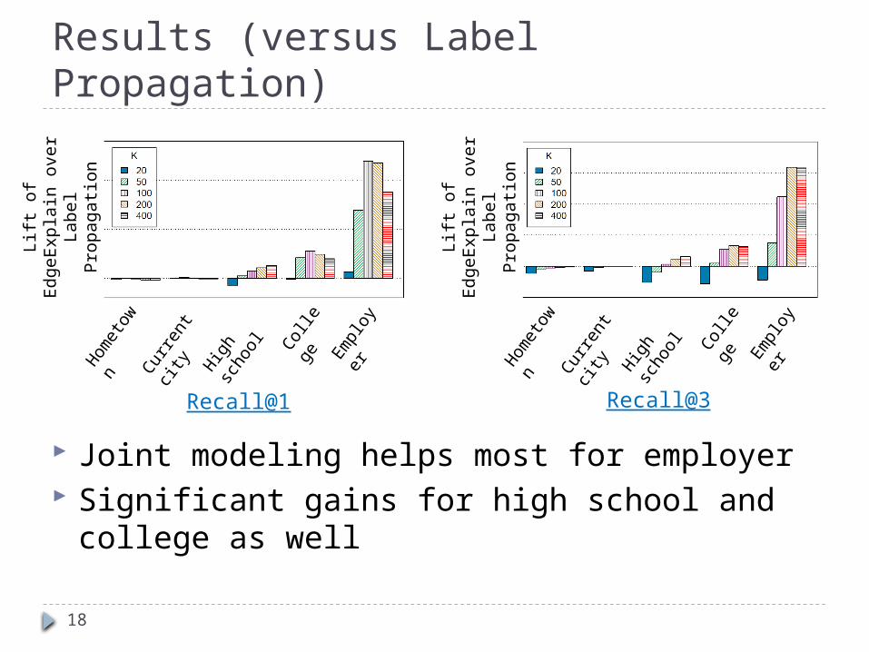
Results (versus Label Propagation)

Joint modeling helps most for employer Significant gains for high school and college

as well

Hom

eto

wn Cu

rren

t ci

ty Hig

h sc

hool Co

llege Em

ploy

er

Lift

of

EdgeExp

lain

over

Label

Pro

pag

ati

on

Hom

eto

wn Cu

rren

t ci

ty Hig

h sc

hool Co

llege Em

ploy

er

Lift

of

EdgeExp

lain

over

Label

Pro

pag

ati

on

Recall@1 Recall@3

19

Conclusions Assumption: each friendship has one reason Model: explain friendships via user attributes Results: up to 120% lift for recall@1 and 60%

for recall@3

20

Result (effect of α)

High α is best one reason per friendship is enough

Lift

of

Ed

geE

xp

lain

over

α=

0.1

Hom

etow

n Curren

t ci

ty Hig

h sc

hool Co

lleg

e Empl

oyer

21

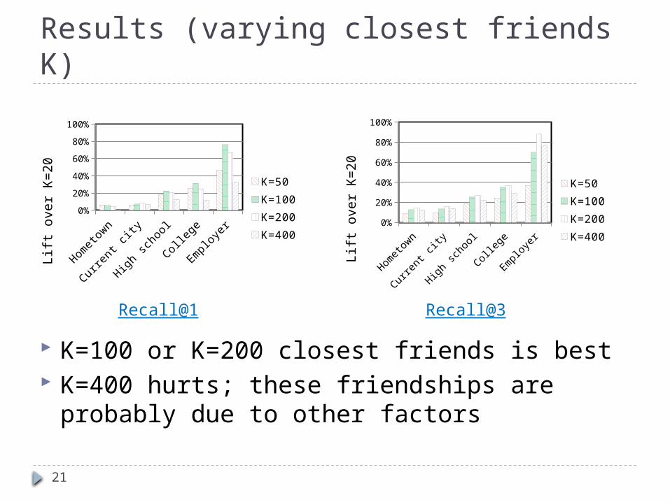
Results (varying closest friends K)

K=100 or K=200 closest friends is best K=400 hurts; these friendships are probably

due to other factors

Homet

own

Curre

nt city

High

scho

ol

College

Employ

er0%

20%

40%

60%

80%

100%

K=50K=100K=200K=400

Lif

t o

ve

r K

=2

0

Homet

own

Current c

ity

High s

choo

l

College

Emplo

yer

0%

20%

40%

60%

80%

100%

K=50K=100K=200K=400

Lif

t o

ve

r K

=2

0

Recall@1 Recall@3

22

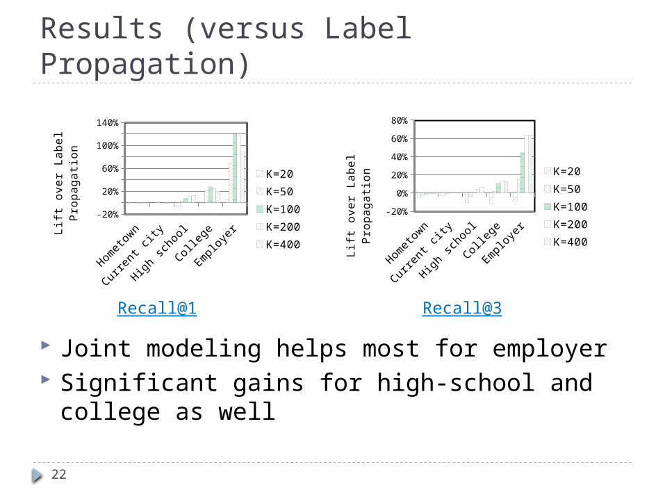
Results (versus Label Propagation)

Joint modeling helps most for employer Significant gains for high-school and college

as well

Homet

own

Curre

nt city

High

scho

ol

College

Employ

er-20%

0%

20%

40%

60%

80%

100%

120%

140%

K=20K=50K=100K=200K=400

Lift

ove

r La

bel P

ropaga-

tion

Homet

own

Curre

nt city

High

scho

ol

College

Employ

er-20%

0%

20%

40%

60%

80%

K=20K=50K=100K=200K=400

Lift

ove

r La

bel P

ropaga-

tion

Recall@1 Recall@3