Joint Discussion Paper

Series in Economics

by the Universities of

Aachen ∙ Gießen ∙ Göttingen Kassel ∙ Marburg ∙ Siegen

ISSN 1867-3678

No. 29-2017

Reinhold Kosfeld and Christian Dreger

Towards an East German wage curve – NUTS boundaries, labour market regions and unemployment spillovers

This paper can be downloaded from

http://www.uni-marburg.de/fb02/makro/forschung/magkspapers

Coordination: Bernd Hayo • Philipps-University Marburg

School of Business and Economics • Universitätsstraße 24, D-35032 Marburg Tel: +49-6421-2823091, Fax: +49-6421-2823088, e-mail: hayo@wiwi.uni-marburg.de

1

Towards an East German wage curve - NUTS boundaries, labour market regions and unemployment spillovers Reinhold Kosfeld1 and Christian Dreger2 Abstract. The relevance of spatial effects in the wage curve can be rationalized by

the model of monopsonistic competition in regional labour markets. However,

distortions in extracting the regional unemployment effects arise in standard regional

(i.e. NUTS) classifications as they fail to adequately capture spatial processes. In

addition, the nonstationarity of wages and unemployment is often ignored. Both

issues are particularly important in high unemployment regimes like East Germany

where a wage curve is difficult to establish. In this paper, labour market regions

defined by economic criteria are used to examine the existence of an East German

wage curve. Due to the nonstationarity of spatial data, a global panel cointegration

approach is adopted. By specifying a spatial error correction model (SpECM),

equilibrium adjustments are investigated in time and space. The analysis gives

evidence on a locally but not a spatially cointegrated wage curve for East Germany.

Key Words: Wage curve, labour market regions, global cointegration, spatial error-

correction model

JEL classification: J30, J60, C33, R15

1. Introduction

Since the discovery of the wage curve by Blanchflower and Oswald (1990, 1994,

1995) in the early 1990s, a large strand of the literature has been devoted to this

topic. Blanchflower and Oswald (1995) present evidence for a negative relationship

between wages and the regional unemployment rate. Such a curve can be

rationalized by profit maximization in non-competitive markets. One explanation of

why a worker living in a high unemployment area earns less than a jobholder with the

same individual characteristics in an area of low unemployment is given by the

efficiency wage model (cf. Blanchflower and Oswald 1994; Card 1995). Employers

1 University of Kassel, Institute of Economics 2 German Institute of Economic Research (DIW Berlin) and European University Viadrina Frankfurt (Oder)

2

have the opportunity to lower the efficiency premium when outside options of workers

are reduced in deteriorating labour markets.

Blanchflower and Oswald (1994) detected a stable elasticity of wages with respect to

unemployment of around -0.10 for a number of countries and periods. However, this

“empirical law of economics” (Card 1995) could not be confirmed by follow-up

studies. Although the difference to the bias-corrected estimate of -0.07 of Nijkamp

and Poot (2003) is small, their meta-study shows considerable heterogeneity among

estimated wage curve elasticities. Even after excluding outliers, elasticities vary

between -0.50 and +0.10. Non-unique results are also striking in the German case.

Controlling for regional fixed effects Wagner (1994) does not find a significant

relationship between wages and unemployment for West Germany in the second half

of the 1980s. Similarly, Pannenberg and Schwarze (1998) fail to detect a standard

wage curve for East Germany in the early 1990s. In contrast, after controlling for

endogeneity of the unemployment rate, the study of Baltagi, Blien and Wolf (2000) is

favourable to the existence of an East German wage curve in the 1990s.

Pannenberg and Schwarze (2000) investigate the wage curve for West Germany at

the regional level for a period of five years before and after the German unification.

From an error correction framework, a dynamic autoregressive wage curve equation

is derived with region- and time-specific fixed effects. While there is evidence for an

inverse relationship between wages and unemployment in the long-run, substantial

inertia occurs in the short-run. Nonetheless, the outcome supports the existence of a

long-run relationship between wages and unemployment with partial adjustment

towards the long run equilibrium. The cointegration approach of Ammermüller et al.

(2010) confirms a weakly significant negative long-run effect of regional

unemployment on wages with partial adjustment. These results are in line with the

analysis of Baltagi, Blien and Wolf (2009) who revealed a wage curve for West

Germany with substantial autoregressive behaviour.

Previous studies are often plagued by serious deficts. For instance, inconsistent

parameter estimates may arise from ignoring the endogeneity of the unemployment

rate. Moreover, labour market conditions in surrounding regions are often excluded

and may constitute an omitted variable bias (cf. Greene 2011, p. 386). Longhi,

Nijkamp and Poot (2004) refer to the theory of monopsonistic competition to justify

the presence of unemployment spillovers in the wage function. If commuting costs to

3

workplaces outside the home region are relatively low, working conditions in

neighbouring regions will likely affect the bargaining power of workers and

employers. In contrast to Büttner (1999), Longhi, Nijkamp and Poot (2004) do not find

an inverse effect of unemployment in neighbouring regions on local wages for West

Germany. Büttner (1999) discovers even a higher unemployment elasticity in

absolute value if larger labour markets are considered. This finding is corroborated by

the recent studies of Fingleton and Palombi (2013) and Kosfeld and Dreger (2017) at

the district level. Baltagi, Blien and Wolf (2012) argue that myopic behaviour of

agents in labour markets is a possible explanation for the lack of unemployment

spillovers. In their spatial approach to the East German wage curve, Elhorst, Blien

and Wolf (2007) discuss a test structure for estimating the wage curve elasticity

without unemployment spillovers. In contrast to Western Germany, evidence on the

role of spatial effects in wage determination and labour market adjustment is scarce

for East Germany. Regional labour markets are still very distinct in both areas, with

respect to labour supply, labour productivity, wages, unemployment, bargaining

coverage and union density (Schnabel 2016).

This paper investigates the relationship between wages and unemployment for East

German regions over the period of 1995 to 2010. The East-West divide in the levels

of wages and unemployment is a cogent cause for not mixing data sets of both parts

of the economy. Responses of wages to changes in unemployment are expected to

differ under diverse labour market conditions. In slack labour markets very limited

wage cuts may not necessarily cause workers to quit their jobs. Large scale active

labour market programs were launched in East Germany to support the economic

transformation and to tackle the social consequences of higher unemployment

(Hagen 2003). For these reasons, the existence of an East German wage curve

defines a distinct topic of research (cf. Pannenberg and Schwarze 1998; Baltagi,

Blien and Wolf 2000; Elhorst, Blien and Wolf 2007).

We extend the stock of knowledge in this area in several respects. First, the influence

of labour market conditions in neighbourhood regions on local wages is examined.

Up to now, no results on the role of spatial unemployment spillovers is available for

East Germany. Second, wage dynamics are investigated on the basis of a spatial

error correction model where adjustment to equilibrium is examined with respect to

time and space. This leads to the concepts of global and local cointegration essential

4

for the analysis. Third, we show that the impact of direct and spatial effects may be

seriously biased if the regional units are defined by administrative boundaries.

Therefore, wage curve elasticies should be estimated in the framework of labour

markets delimited by functional criteria.

The paper is structured as follows. Section 2 reviews the literature on the wage curve

with a special focus on the German evidence. Section 3 outlines the concept of the

wage curve extended by spatial effects. The econometric metholology is discussed in

section 4, and the empirical findings are presented in Section 5. Section 6 provides a

sensivity analysis of the results, and Section 7 concludes with some policy

recommendations.

2. Previous studies on the wage curve

The negative relationship between wages and regional unemployment detected by

Blanchflower and Oswald (1994, 1994) claimed a stable unemployment elasticity of

wages of approximately -0.1, independent of the time period and the countries in the

analysis. Since the mid of the 1990s this “empirical law” triggered numerous empirical

studies. A lot of research was done for the German economy. The strand of panel

studies on the German wage curve was launched by the work of Wagner (1994) and

Baltagi and Blien (1998) who provided evidence for the relationship in pre-unification

periods.

After 1990 the analysis of the wage curve is still conducted separately for the

Western and Eastern part of Germany due to substantial differences in economic

conditions. Virtually all studies make use of the same regional and temporal

disaggregation. Annual data for different time periods are analysed for urban and

rural districts according to the NUTS-3 classification of the European Union.3 The

studies differ essentially in the way they cope with multilevel data, the endogeneity

problem, spatial and dynamic effects. The nonstationarity of variables is usually

ignored. For the West German case, wage curves for different groups of workers

have been estimated too.

3 Exeptions are the studies of Pannenberg and Schwarze (1998, 2000) and Ammermüler et al. (2010). While the

former authors make use of employment office districts (‘Arbeitsamtsbezirke‘) and spatial planning regions

(‘Raumordnungsregionen‘) within the territory of the states (the German ‘Länder‘) as spatial units, the latter

work relies on state level data.

5

Pannenberg and Schwarze (1998) estimate the wage curve for Eastern Germany

with data drawn from the German Socio Economic Panel over the 1992–94 period.

After linking individual data to the 35 labour office districts a negative employment

elasticity is found in a pooled OLS model with fixed regional effects. However,

feasible GLS estimation of a panel model with random individual and regional fixed

effects does not confirm the finding, as the negative relationship is no longer

significant. After replacing the unemployment rate by the regional job search rate the

authors find a wage curve elasticity of -0.14 which is significant at the 5% level. The

broader measure of labour market slack is used to account for large scale active

labour market programs. The elasticity declines to -0.53, if simultaneity bias is taken

into account.

As the study of Pannenberg and Schwarze (1998) is restricted to a short period at the

start of transition of a centrally planned economy to a market economy, one can

scarcely interpret their finding in favour a long-run relationship between wages and

regional unemployment. Excluding the first two transition years from their sample,

Baltagi, Blien and Wolf (2000) examine the existence of an East German wage curve

over the 1993–98 period. Using regional unemployment rates of the 114

administrative districts, the effective sample size is increased considerably. On the

basis of the two-ways fixed effects estimator the wage curve is not supported. The

picture changes when the unemployment rate is instrumented by exogenous

regressors and their lagged values. After controlling for endogeneity of the

unemployment rate in this way, first-difference 2SLS estimation yields a highly

significant overall unemployment elasticity of -0.15.

Regions usually refer to administrative boundaries. Büttner (1999) argues that the

neighbouring regions may be related through common shocks and activities of

agents operating in larger labour markets. In his investigation of West German wages

in manufacturing industry over the 1987-94 period he shows a downward bias of the

estimated unemployment elasticity of wages if spatial effects are neglected. Using

the inverse unemployment rate as a regressor in a restricted fixed-effects spatial

Durbin model, it is found that regional wages respond to variations in the regional

unemployment rate with decreasing extent. For the 327 West German districts, the

estimated elasticities are in the range of -0.040 to -0.005 in the non-spatial case and

-0.053 to -0.008 in the spatial case.

6

Longhi, Nijkamp and Poot (2006) introduce spatial effects into the wage curve by

drawing on monopsonistic competition. If employment opportunities in nearby regions

are available to workers, the threat of unemployment will decrease. Employees are

aware of economic conditions in surrounding areas. However, as workers face

commuting and migration costs, employers will have some degree of monopsonistic

power. In their study of the West German wage curve over the 1990–97 period,

Longhi, Nijkamp and Poot (2006) show the importance of spatial effects for the 327

NUTS-3 regions. Due to the interaction of the unemployment rate with an index of

accessibility and agglomeration, the estimated wage elasticity varies with the

unemployment level. However, 2SLS fixed-effect estimation of a simplified model

without quadratic terms gives evidence for a negative elasticity around -0.02.

Interpretation problems occur as the sign of the spatially lagged unemployment rate

is positive, in contrast to expectations.

In estimating the East German wage curve for period 1993–99 period, Elhorst, Blien,

and Wolf (2007) focus on the treatment of potential endogeneity in spatial panel

models with time-specific effects. Their testing strategy is as well applicable to

region-specific effects. For a panel of 114 East German districts, different estimators

of the unemployment elasticity are compared. After establishing regional

unemployment rates not to be strictly exogenous, 2SLS with temporal and spatial

differences in the presence of fixed effects is preferred. The estimator corroborates

the wage curve hypothesis for East German with an elasticity value of -0.039 that is

significant at the 5% level.

Dynamic effects in the wage curve are often neglected. For West Germany,

Pannenberg and Schwarze (2000) provide in their analysis of 74 regions over the

period 1985-94 evidence on inertia of regional wages in the short-run. For the

Arellano-Bond estimator, a highly significant value for the autoregressive parameters

of 0.30 results. In the long-run, a negative equilibrium relationship between wages

and unemployment is established. The estimated wage elasticity with respect to

unemployment of -0.04 is low in absolute value but significant. Spatial effects have

not been included.

Ammermüller et al. (2010) adopt a cointegration approach in investigating the wage-

unemployment nexus for Italy and Germany. For Germany, panel analysis is based

on microcensus data on net income and individual characteristics in combination with

7

state level unemployment rates. Spatial spillovers are ignored, as the administrative

regions are quite large. Fixed effect estimation fails to confirm the wage curve

hypothesis for West Germany for 1996–2003. In contrast, a significant negative

relationship between wages and regional unemployment is established for East

Germany employees, females and low educated workers.

Baltagi, Blien and Wolf (2012) investigate the wage curve relationship for West

Germany over the period 1980-2004 with individual wage data covering all 326

NUTS-3 regions. Lagged wages are embedded to control for dynamic effects. The

presence of regional unemployment spillovers is tested using different spatial weights

matrices. After instrumenting the unemployment rate and its spatial lag by their time

lags, a highly significant and robust long-run wage curve elasticity of about -0.04 is

inferred for West Germany. In virtually all cases, spatial effects arising from

unemployment are not detected. The signficance of the autoregressive parameter

corroborates the dynamic specification of the wage curve.

The recent study of Kosfeld and Dreger (2017) on the relationship between wages

and unemployment focuses on West Germany. The work integrates spatial effects in

a panel cointegration framework. Using panel data for 325 NUTS-3 regions over the

period 1995-2005, a stable long-run wage curve with spatial effects is found. The

unemployment spillover effect turns out to be even stronger than the local impact of

unemployment on wages. However, the instrumental variable (IV) estimator of the

unemployment elasticity is below one-tenth of the value suggested by Blanchflower

and Oswalds’s (1995, 2005) empirical law.

3. The concept of the wage curve

The wage curve postulates a negative relationship between the wage rate of workers

and the regional unemployment rate. The standard approach renders the relationship

between individual wages, wirt, and the regional unemployment rate, urt, controlled by

a set of individual characteristics X1irt, X2irt, …, Xmirt as well as region and time fixed

effects, r, and t, respectively:

(1) irtjirt

m

1jjrttrirt εXδ)log(uβαα)log(w

8

The parameter denotes the unemployment elasticity and the parameters are the

regression coefficients of control variables like age, gender, education, industry and

firm size. Finally, irt is an idiosyncratic disturbance.

Competitive models of the labour market fail to explain the negative association

between individual wages and regional unemployment (Blanchflower and Oswald

1995; Card 1995). Thus, the wage curve is based on non-competitive market

structures. A negative linkage between unemployment and wages could be explained

by the labour contract and union bargaining models. Although pacts of employment

and competitiveness relieved wage agreements at the firm level in Germany (Seifert

and Massa-Wirth 2005), collective bargaining is still dominant (Fitzenberger, Kohn

and Lembcke 2013). However, collective agreements refer to the industrial, not to the

regional level (Fitzenberger, Kohn and Lembcke 2013).

The efficiency wage hypothesis provides an explanation of wages that is not linked to

a particular institutional setting. According to the model proposed by Shapiro and

Stiglitz (1984), employers offer wage premiums to promote workers’ efforts and avoid

shirking. The higher the unemployment rate, the more difficult workers will find a new

job in case of a dismissal. Against this backdrop, firms can afford to offer lower wage

premiums in slack labour markets. Therefore, a negative link between regional

unemployment and wages is expected. With the labour turnover model (Campbell

and Orszag 1998) as a special variant of the efficiency wage hypothesis, the wage

curve is drawn on fixed costs for recruiting and training. As these costs might be

rather high, employers will accept a premium on top of the bill to keep current

employees and discourage them to quit. Wage premiums will be lower in periods of

economic downturns, where it is less likely that workers quit and find new jobs.

Both the efficiency wage hypothesis and the labour turnover model can be adopted

into a system of interacting regions (Longhi, Nijkamp and Poot 2006). The power of

threat of shirking or quitting to workers is not only represented by local labour market

conditions but also by the unemployment rate in proximate regions (Fingleton and

Palombi, 2013). The regional dimension is introduced by monopsonistic competition.

In view of commuting flows across regions, local labour markets cannot be longer

treated as isolated entities. In the presence of spatial interactions among

neighbouring territories, competition for workers takes place within and between

proximate labour market areas. Thus, local wages wrt are determined by

9

unemployment in the own and neighbouring regions, urt and SL(urt), after controlling

for individual characteristics Xjrt and region and time fixed effects:

(2) irtjirt

m

1jjrtrttrirt εXδ))SL(log((u*β)log(uβαα)log(w

The spatial spillover unemployment elasticity of pay, *, measures the effect of the

spatially weighted unemployment rate of proximate regions, ))SL(log((urt , on the own

region’s wage rate. The spillover variable ))SL(log((urt is operationalized with the aid

of a matrix of spatial weights *. Here, the contiguity concept is employed, where

*rsω is set equal to 1 if the regions r and s, r≠s, share a common boundary and 0

otherwise. As arobustness check, we also use spatial weights corresponding to travel

time between the regions. s. Using row-standardized weights rsω (Anselin and Bera

1998, p. 243), the spatial lag of the unemployment rate can be written as

)log(uω))SL(log((un

1sstrsrt

.

4. Global cointegration and spatial error correction

The variables in the standard and spatial wage curve (1) and (2) are measured for

different types of statistical units. While the wage wirt refers to individuals, the

unemployment rate urt relates to regions. Adverse effects occur when workers in the

same labour market share common components of variance reflected in explanatory

variables and disturbances. In this case, the errors irt will be positively autocorrelated

across individuals in the same labour market. Due to the common group effect, the

standard error of the response coefficients will be downward biased (Moulton 1990).

To account for the Moulton bias, usually individual aggregation is conducted when

spatial effects come into play, regardless of the estimation strategy (Baltagi, Blien

and Wolf 2012). Here the common group effect is addressed by averaging individual-

specific variables over all workers in labour market r in period t:

(3) rtjrt

m

1jjrtrttrrt εXδ))SL(log((u*β)log(uβαα)log(w

.

10

In this specification, the control variables of the spatial wage curve (3), X1rt, X2rt, …,

Xmrt, reflect observable regional characteristics. To account for omitted variables that

are correlated across space, a spatially autocorrelated error process can be adopted:

(4) rtrt

m

1jrsrt εwρε ν

where rt is an i.i.d. innovation. The equations (3) and (4) constitute a fixed effects

SLX panel model with spatially autocorrelated errors (FE-SLX-SEM model). For =0

the FE-SLX panel model arises. The case *=0 and =0 typifies the standard FE

panel model.4

Another problem will occur due to the endogeneity of the unemployment rate. From

the standard FE panel model it is known that the unemployment elasticity will be

downwardly biased and inconsistent in this case (Baltagi and Blien 1998; Baltagi,

Baskaya and Hulago 2012). Baltagi and Blien (1998) show that the wage curve

elasticity is indeed sensitive to endogeneity. To avoid the resulting bias, the regional

unemployment rate should be instrumented with time lags of the unemployment rate

and the control variables. Specifically, one- and two-period lags of the regional

unemployment rate are chosen jointly with the contemporary and lagged control

variables as instruments.

If the wage curve constitutes a long-run equilibrium relationship, the model (3) can be

interpreted as a cointegrating equation between wages, unemployment and regional

characteristics. By noting the autoregressive nature of wage bargaining, Blanchflower

and Oswald (2005) view “the data as being characterized by dynamic fluctuations

around a long-run wage curve”.

In order to be cointegrated, at least two variables must share the highest order of

integration. Panel unit root tests usually assume independent time series across the

panel members. This assumption is particularly violated in spatial panels. Pesaran

(2007) augmented the IPS test5 by adopting a common factor model for capturing

cross-sectional dependence. By additionally accounting for serial dependence in

form of an AR(1) error process, the test equation for the variable y without a

deterministic trend reads

4 SLX stands for spatial lag of one or more explanatory variables. For a taxonomy of spatial panel data

models s. Elhorst (2014, pp. 37 with reference to p. 9). 5 The IPS test is a test on the presence of a unit root in heterogenous panels without accounting for cross-

sectional dependence (Im, Pesaran and Shin 2003).

11

(5) rt1t,rr1t1rt0r1tr1t,rrrrt uyeydydycybay .

In this approach, the common factor is proxied by the cross-section mean ty and its

lagged value. For non-trended data the cross-sectionally augmented IPS test (CIPS

test) already has satisfactory size and power for moderate values of n and T. For

trended data, however, the power of the test starts to raise with n only for T>30.

Recent studies on the wage-unemployment nexus discovered not only the relevance

of spatial effects but also a central role of wage inertia (Baltagi, Blien and Wolf 2009,

2012; García-Mainar and Montuenga-Gómez 2012; Ramos, Nicodemo and Sanroma

2015). Although Blanchflower and Oswald (1995) already pointed to error-correction

models as suitable tools to distinguish between short run dynamics and a long-run

equilibrium, studies usually introduce dynamics by adding lagged wages and

unemployment rates. The notion of modelling inertia of wage adjustment by an error

correction mechanism (ECM) in a regional setting has been taken up by

Ammermüller et al. (2012). However, spatial effects are usually neglected. While

adjustments to equilibrium wages within the regions are considered, the between

effects are excluded.

Recently, Beenstock and Felsenstein (2010, 2015) extended the standard panel error

correction model by “spatializing” the adjustment to equilibrium. The error-correction

mechanism is assumed to work not only within but also between the regions. While

the effectiveness of local error correction is examined by the coefficient of the lagged

residuals 1-tr,EC from the long–run relationship, the presence of spatial correction is

assessed by evaluating the coefficient of the lagged residuals of neigbouring regions

*1-tr,EC . The spatial error correction model (SpECM) additionally captures changes in

labour market conditions in the neighbourhood regions. The dynamic counterpart of

the cointegrating relationship (3) reads

(6) ))ΔSL(log(u))Δ(log(u))Δ(log(u))Δ(log(wα))Δ(log(w rt1-tr,rt1-tr,rt*0101

rt*

1-tr,1-tr,

m

1j1-tjr,j1

m

1jjrtj01-tr, EC*ααECΔXθΔXθ))ΔSL(log(u ν

*1

based on an autoregressive distributed lag model (ADL) of order 2 in the dependent

and explanatory variables. For local error correction to be effective, the adjustment

coefficient should be negative. In this case, previous deviations from local

12

equilibrium wages are partially reduced in the following periods. Spatial error

correction relates to equilibrium adjustment across space. A positive sign of the error

correction coefficient * indicates the effectiveness of an adjustment process

between proximate regions. Both coefficient and * measure the speed of

adjustment toward long-run equilibrium. For - 1<0 and 0<*1 the system is said

to be globally cointegrated. In case of a negative spatial adjustment coefficient *,

above-equilibrium wages in the neighbouring regions would exert a downward

pressure on local wages. The borderline case =*=1 indicates full adjustment within

one period. In the special case =*=0, the spatial error correction model (SpECM)

turns into a spatial vector autoregression as an adequate dynamic modelling

framework for stationary variables.

In the SLX fixed effects panel model with spatially autocorrelated errors, OLS

produces inefficient estimates of the regression coefficients (Anselin 1988, p. 59;

LeSage and Pace 2009, p. 62). By taking the Jacobian determinant into account,

maximum likelihood (ML) may provide efficiency gains (cf. LeSage and Pace 2010, p.

359). This also holds for the ML approach applied to the spatial panel model with

fixed effects (see e.g. Elhorst 2010, p. 393). The problem of a simultaneity bias in the

case of reverse causality is usually adressed by instrumental variables (IV).

However, the proposed methods are not optimally designed for nonstationary data. In

a spatial analysis the number of regions is usually fixed as the spatial units are not

sampled (Elhorst 2014, pp. 55-56). Suppose the observable variables of a spatial

panel model are integrated of order one (I(1)) and cointegrated. In this case, the

nonstationary regressors are asymptotically independent from the stationary I(0) error

term (Beenstock and Felsenstein 2015). Although OLS estimators are super-

consistent, the simultaneity bias is still present in finite samples. Given the fixed

number of regions, the finite sample bias depends just as asymptotics on the number

of periods, T. To address this bias, potentially endogenous regressors may be

instrumented.

In their global cointegration analysis of Israel’s housing market, Beenstock and

Felsenstein (2015) provide arguments that the endogeneity bias is negligible with a

sample size of T=24 for annual data. In the 2010 paper they use OLS with T=18

without any instrumentation in estimating the long-run relationship and the SpEC

model. However, up to now, reliable knowledge on finite sample properties of panel

13

cointegration is not available. In their analysis of productivity growth across Chinese

provinces, Mitze and Oezyurt (2014) account for the endogenity of the spatially

lagged dependent variable by applying the ML approach of Lee and Yu (2010a) even

with a larger sample size of T=33. Kosfeld and Dreger (2017) apply the ML-IV

method to allow for the simultaneity bias in studying the West German wage curve

with an effective sample size of T=15.

In this paper, the panel cointegration analysis of the East German wage curve is

conducted for both 77 administrative and 33 functional regions over a 16-year period.

By making use of one- and two period lagged variables to account for partial

adjustment patterns the effectively number of observations per spatial unit reduces to

T=14. With this number of time periods the endogeneity bias deserves more attention

than in the aforementioned studies. For that reason, the long-run wage curve is

estimated by applying the ML and OLS methods on a set of nonstationary variables

with an instrumented unemployment rate as a potentially endogenous regressor.

Besides the one- and two-period lagged unemployment rate, contemporaneous and

lagged control variables are used as instruments. To check the extent of a

simultaneity bias, the estimation is also performed without instrumentation.

In the SpEC model the log difference of the wage rate is regressed on one-period

lagged first- and second-order differenced explanatory variables and local and spatial

error correction (EC) terms. As all differenced variables are stationary the

simultaneity bias matters even asymptotically. Thus, the use the instrumental

variables (IV) technique is invariably indicated here in the presence of endogenous

regressors. Again the consequences of instrumentation on relevant parameter

estimates is checked.

5. Defining regional areas

In almost all studies, panel data on small administrative regions like districts are

employed to estimate the wage curve. As these areas usually do not constitute

separate labour markets, spatial effects are expected to be present. However,

administrative units do not adequately reflect the scale of the underlying spatial

process. Thus, in analysing spatial data from administrative regions, substantial

spillovers will be confounded by error dependence evoked due to measurement

problems. They can be avoided by using functional defined areas. Labour market

14

regions are characterized by commuter flows, where the commuting distance can

serve as a delimiter (cf. Kosfeld and Werner 2012; Kropp and Schwengler 2016). We

particularly draw on the factor analytic approach of Kosfeld and Werner (2012) who

extract labour market regions from the correlation structure of commuter flows across

German districts. To improve the connectedness of the functional areas, the

commuting distance is considered as a constraint. The commuting distance within

employment areas is limited to politically acceptable thresholds between 45 to 60

minutes travel time dependent on the attractiveness of the centres. In this way, 33

labour market regions consisting of one up to six districts are extracted from the 77

East German districts (NUTS-3 regions).

Unemployment rates are measured for both districts and employment agencies. The

administrative districts are the smallest spatial units for which unemployment rates

are reported. Because of their embeddedness in the competences and

responsibilities of the public employment administration (Hilbert 2008, pp. 73-74),

regions corresponding to employment agencies do not share the characteristics of

functional regions (Kropp and Schwengler 2016). Yearly panel data on

unemployment for the 77 East German NUTS-3 regions are available from the

Labour Market Statistics of the German Federal Employment Agency (BA).

Unemployment rates for the functional labour market regions are obtained through

averaging the corresponding unemployment rates in the districts, where labour force

weights are used.

The official statistics provides different indicators for wages. The Regional Database

of the German Federal Statistical Office reports gross wages and salaries per year.

By dividing through the number of employees, annual wages per worker are

obtained. However, without calculating full-time equivalents, full time and part time

occcupations will be mixed. Daily wages drawn from the Sample of Integrated Labour

Market Biographies (SIAM) of Integrated Employment Biographies (IEB) of the

Institute for Employment Research (IAB) relate to full-time employees with hourly

wages of more than six Euro who are subject to social security contributions.

In investigating the impacts of economic conditions on wages, individual

characteristics like vocational education, experience and gender have to be included

(cf. Heckman, Lochner and Todd 2003). In addition, working time, branch and firm

size may influence hourly wages. Data on the control variables is provided at the

15

district level by the Federal Employment Agency. The variables at the level of

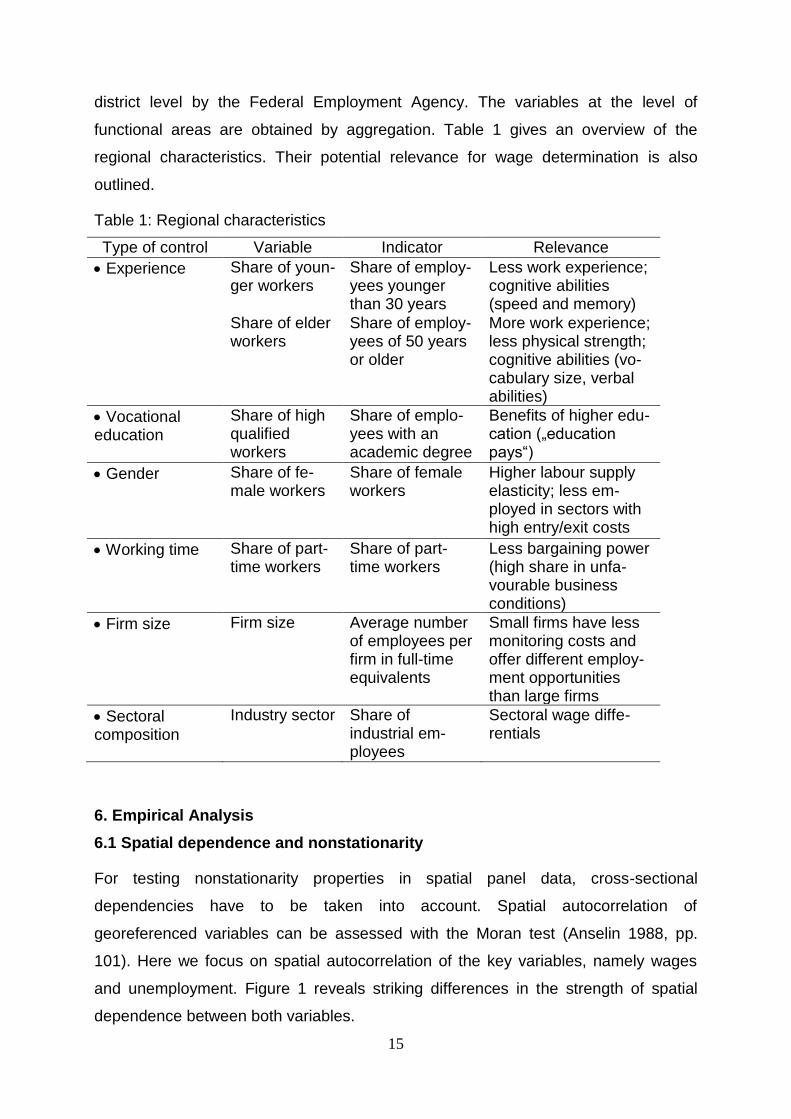
functional areas are obtained by aggregation. Table 1 gives an overview of the

regional characteristics. Their potential relevance for wage determination is also

outlined.

Table 1: Regional characteristics

Type of control Variable Indicator Relevance

Experience Share of youn-ger workers

Share of employ-yees younger than 30 years

Less work experience; cognitive abilities (speed and memory)

Share of elder workers

Share of employ-yees of 50 years or older

More work experience; less physical strength; cognitive abilities (vo-cabulary size, verbal abilities)

Vocational education

Share of high qualified workers

Share of emplo-yees with an academic degree

Benefits of higher edu-cation („education pays“)

Gender Share of fe-male workers

Share of female workers

Higher labour supply elasticity; less em-ployed in sectors with high entry/exit costs

Working time Share of part-time workers

Share of part-time workers

Less bargaining power (high share in unfa-vourable business conditions)

Firm size Firm size Average number of employees per firm in full-time equivalents

Small firms have less monitoring costs and offer different employ-ment opportunities than large firms

Sectoral composition

Industry sector Share of industrial em-ployees

Sectoral wage diffe-rentials

6. Empirical Analysis

6.1 Spatial dependence and nonstationarity

For testing nonstationarity properties in spatial panel data, cross-sectional

dependencies have to be taken into account. Spatial autocorrelation of

georeferenced variables can be assessed with the Moran test (Anselin 1988, pp.

101). Here we focus on spatial autocorrelation of the key variables, namely wages

and unemployment. Figure 1 reveals striking differences in the strength of spatial

dependence between both variables.

16

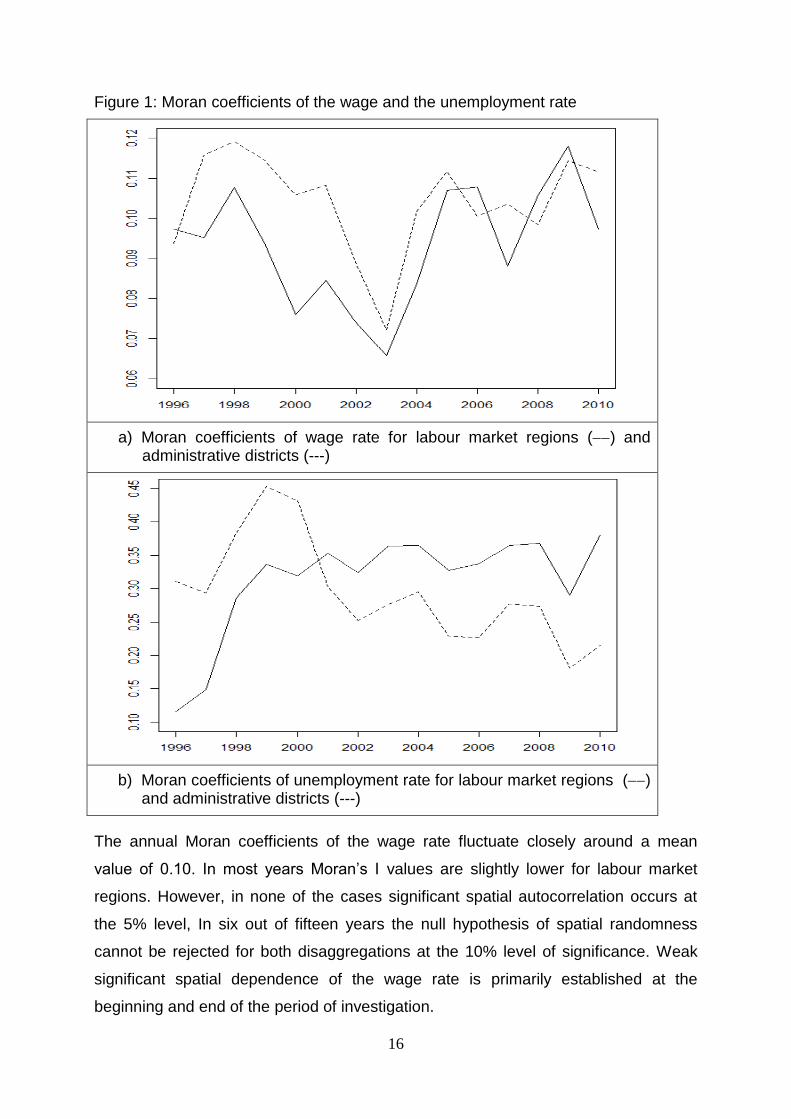
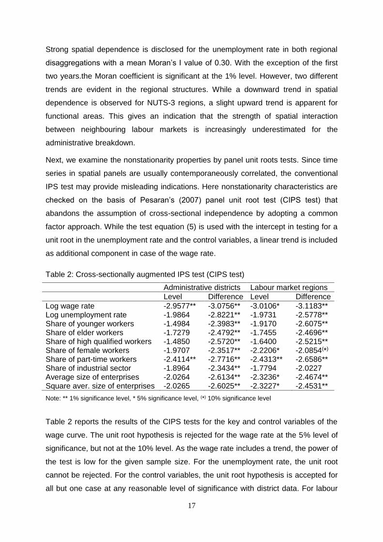
Figure 1: Moran coefficients of the wage and the unemployment rate

a) Moran coefficients of wage rate for labour market regions () and administrative districts (---)

b) Moran coefficients of unemployment rate for labour market regions () and administrative districts (---)

The annual Moran coefficients of the wage rate fluctuate closely around a mean

value of 0.10. In most years Moran’s I values are slightly lower for labour market

regions. However, in none of the cases significant spatial autocorrelation occurs at

the 5% level, In six out of fifteen years the null hypothesis of spatial randomness

cannot be rejected for both disaggregations at the 10% level of significance. Weak

significant spatial dependence of the wage rate is primarily established at the

beginning and end of the period of investigation.

17

Strong spatial dependence is disclosed for the unemployment rate in both regional

disaggregations with a mean Moran’s I value of 0.30. With the exception of the first

two years.the Moran coefficient is significant at the 1% level. However, two different

trends are evident in the regional structures. While a downward trend in spatial

dependence is observed for NUTS-3 regions, a slight upward trend is apparent for

functional areas. This gives an indication that the strength of spatial interaction

between neighbouring labour markets is increasingly underestimated for the

administrative breakdown.

Next, we examine the nonstationarity properties by panel unit roots tests. Since time

series in spatial panels are usually contemporaneously correlated, the conventional

IPS test may provide misleading indications. Here nonstationarity characteristics are

checked on the basis of Pesaran’s (2007) panel unit root test (CIPS test) that

abandons the assumption of cross-sectional independence by adopting a common

factor approach. While the test equation (5) is used with the intercept in testing for a

unit root in the unemployment rate and the control variables, a linear trend is included

as additional component in case of the wage rate.

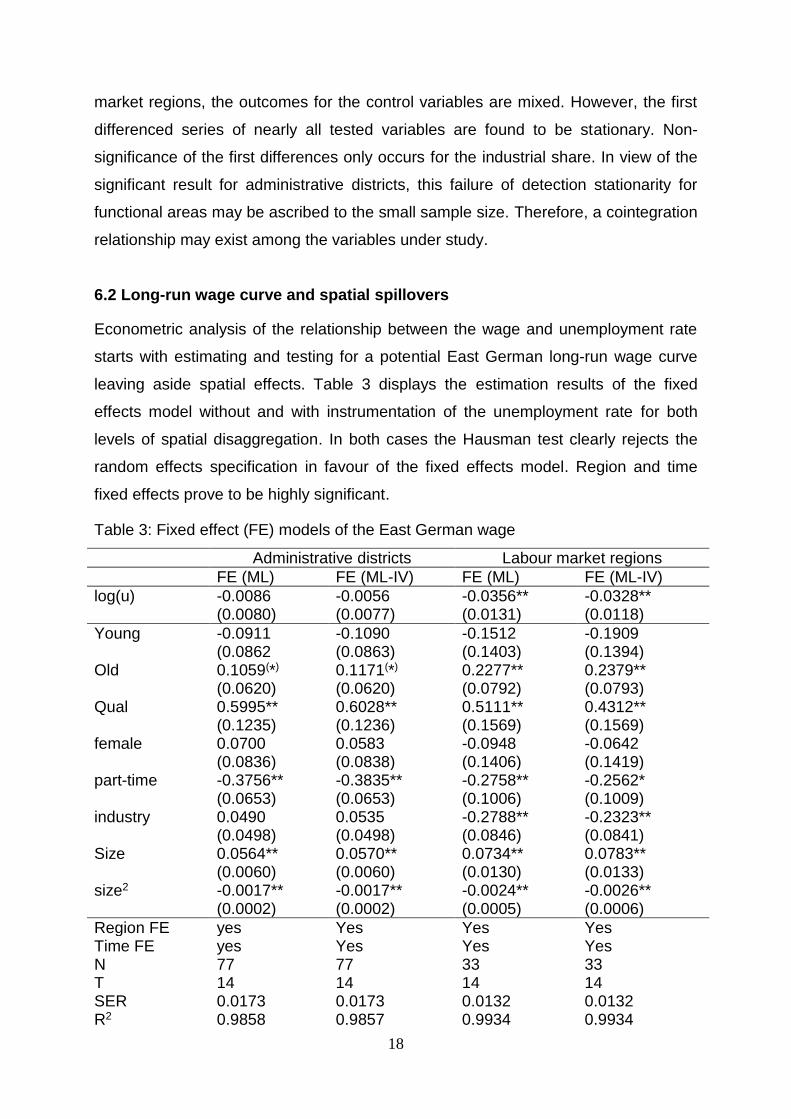
Table 2: Cross-sectionally augmented IPS test (CIPS test)

Administrative districts Labour market regions

Level Difference Level Difference

Log wage rate -2.9577** -3.0756** -3.0106* -3.1183** Log unemployment rate -1.9864 -2.8221** -1.9731 -2.5778** Share of younger workers -1.4984 -2.3983** -1.9170 -2.6075** Share of elder workers -1.7279 -2.4792** -1.7455 -2.4696** Share of high qualified workers -1.4850 -2.5720** -1.6400 -2.5215** Share of female workers -1.9707 -2.3517** -2.2206* -2.0854(*) Share of part-time workers -2.4114** -2.7716** -2.4313** -2.6586** Share of industrial sector -1.8964 -2.3434** -1.7794 -2.0227 Average size of enterprises -2.0264 -2.6134** -2.3236* -2.4674** Square aver. size of enterprises -2.0265 -2.6025** -2.3227* -2.4531**

Note: ** 1% significance level, * 5% significance level, (*) 10% significance level

Table 2 reports the results of the CIPS tests for the key and control variables of the

wage curve. The unit root hypothesis is rejected for the wage rate at the 5% level of

significance, but not at the 10% level. As the wage rate includes a trend, the power of

the test is low for the given sample size. For the unemployment rate, the unit root

cannot be rejected. For the control variables, the unit root hypothesis is accepted for

all but one case at any reasonable level of significance with district data. For labour

18

market regions, the outcomes for the control variables are mixed. However, the first

differenced series of nearly all tested variables are found to be stationary. Non-

significance of the first differences only occurs for the industrial share. In view of the

significant result for administrative districts, this failure of detection stationarity for

functional areas may be ascribed to the small sample size. Therefore, a cointegration

relationship may exist among the variables under study.

6.2 Long-run wage curve and spatial spillovers

Econometric analysis of the relationship between the wage and unemployment rate

starts with estimating and testing for a potential East German long-run wage curve

leaving aside spatial effects. Table 3 displays the estimation results of the fixed

effects model without and with instrumentation of the unemployment rate for both

levels of spatial disaggregation. In both cases the Hausman test clearly rejects the

random effects specification in favour of the fixed effects model. Region and time

fixed effects prove to be highly significant.

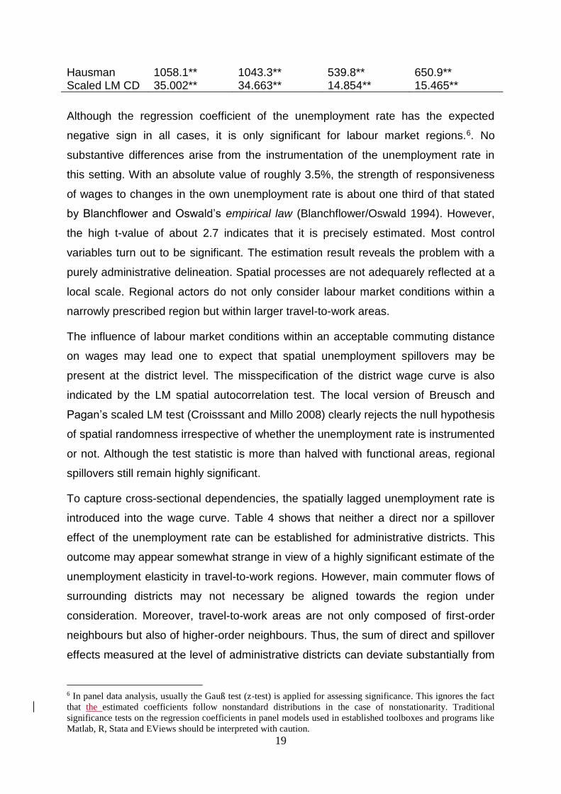
Table 3: Fixed effect (FE) models of the East German wage

Administrative districts Labour market regions

FE (ML) FE (ML-IV) FE (ML) FE (ML-IV)

log(u) -0.0086 (0.0080)

-0.0056 (0.0077)

-0.0356** (0.0131)

-0.0328** (0.0118)

Young -0.0911 (0.0862

-0.1090 (0.0863)

-0.1512 (0.1403)

-0.1909 (0.1394)

Old 0.1059(*) (0.0620)

0.1171(*)

(0.0620) 0.2277** (0.0792)

0.2379** (0.0793)

Qual 0.5995** (0.1235)

0.6028** (0.1236)

0.5111** (0.1569)

0.4312** (0.1569)

female 0.0700 (0.0836)

0.0583 (0.0838)

-0.0948 (0.1406)

-0.0642 (0.1419)

part-time -0.3756** (0.0653)

-0.3835** (0.0653)

-0.2758** (0.1006)

-0.2562* (0.1009)

industry 0.0490 (0.0498)

0.0535 (0.0498)

-0.2788** (0.0846)

-0.2323** (0.0841)

Size 0.0564** (0.0060)

0.0570** (0.0060)

0.0734** (0.0130)

0.0783** (0.0133)

size2 -0.0017** (0.0002)

-0.0017** (0.0002)

-0.0024** (0.0005)

-0.0026** (0.0006)

Region FE yes Yes Yes Yes Time FE yes Yes Yes Yes N 77 77 33 33 T 14 14 14 14 SER 0.0173 0.0173 0.0132 0.0132 R2 0.9858 0.9857 0.9934 0.9934

19

Hausman 1058.1** 1043.3** 539.8** 650.9** Scaled LM CD 35.002** 34.663** 14.854** 15.465**

Although the regression coefficient of the unemployment rate has the expected

negative sign in all cases, it is only significant for labour market regions.6. No

substantive differences arise from the instrumentation of the unemployment rate in

this setting. With an absolute value of roughly 3.5%, the strength of responsiveness

of wages to changes in the own unemployment rate is about one third of that stated

by Blanchflower and Oswald’s empirical law (Blanchflower/Oswald 1994). However,

the high t-value of about 2.7 indicates that it is precisely estimated. Most control

variables turn out to be significant. The estimation result reveals the problem with a

purely administrative delineation. Spatial processes are not adequarely reflected at a

local scale. Regional actors do not only consider labour market conditions within a

narrowly prescribed region but within larger travel-to-work areas.

The influence of labour market conditions within an acceptable commuting distance

on wages may lead one to expect that spatial unemployment spillovers may be

present at the district level. The misspecification of the district wage curve is also

indicated by the LM spatial autocorrelation test. The local version of Breusch and

Pagan’s scaled LM test (Croisssant and Millo 2008) clearly rejects the null hypothesis

of spatial randomness irrespective of whether the unemployment rate is instrumented

or not. Although the test statistic is more than halved with functional areas, regional

spillovers still remain highly significant.

To capture cross-sectional dependencies, the spatially lagged unemployment rate is

introduced into the wage curve. Table 4 shows that neither a direct nor a spillover

effect of the unemployment rate can be established for administrative districts. This

outcome may appear somewhat strange in view of a highly significant estimate of the

unemployment elasticity in travel-to-work regions. However, main commuter flows of

surrounding districts may not necessary be aligned towards the region under

consideration. Moreover, travel-to-work areas are not only composed of first-order

neighbours but also of higher-order neighbours. Thus, the sum of direct and spillover

effects measured at the level of administrative districts can deviate substantially from

6 In panel data analysis, usually the Gauß test (z-test) is applied for assessing significance. This ignores the fact

that the estimated coefficients follow nonstandard distributions in the case of nonstationarity. Traditional

significance tests on the regression coefficients in panel models used in established toolboxes and programs like

Matlab, R, Stata and EViews should be interpreted with caution.

20

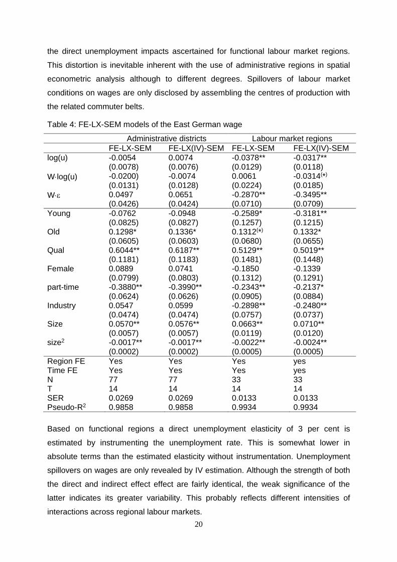
the direct unemployment impacts ascertained for functional labour market regions.

This distortion is inevitable inherent with the use of administrative regions in spatial

econometric analysis although to different degrees. Spillovers of labour market

conditions on wages are only disclosed by assembling the centres of production with

the related commuter belts.

Table 4: FE-LX-SEM models of the East German wage

Administrative districts Labour market regions

FE-LX-SEM FE-LX(IV)-SEM FE-LX-SEM FE-LX(IV)-SEM

log(u) -0.0054 (0.0078)

0.0074 (0.0076)

-0.0378** (0.0129)

-0.0317** (0.0118)

Wlog(u) -0.0200) (0.0131)

-0.0074 (0.0128)

0.0061 (0.0224)

-0.0314(*) (0.0185)

W 0.0497 (0.0426)

0.0651 (0.0424)

-0.2870** (0.0710)

-0.3495** (0.0709)

Young -0.0762 (0.0825)

-0.0948 (0.0827)

-0.2589* (0.1257)

-0.3181** (0.1215)

Old 0.1298* (0.0605)

0.1336* (0.0603)

0.1312(*)

(0.0680) 0.1332* (0.0655)

Qual 0.6044** (0.1181)

0.6187** (0.1183)

0.5129** (0.1481)

0.5019** (0.1448)

Female 0.0889 (0.0799)

0.0741 (0.0803)

-0.1850 (0.1312)

-0.1339 (0.1291)

part-time -0.3880** (0.0624)

-0.3990** (0.0626)

-0.2343** (0.0905)

-0.2137* (0.0884)

Industry 0.0547 (0.0474)

0.0599 (0.0474)

-0.2898** (0.0757)

-0.2480** (0.0737)

Size 0.0570** (0.0057)

0.0576** (0.0057)

0.0663** (0.0119)

0.0710** (0.0120)

size2 -0.0017** (0.0002)

-0.0017** (0.0002)

-0.0022** (0.0005)

-0.0024** (0.0005)

Region FE Yes Yes Yes yes Time FE Yes Yes Yes yes N 77 77 33 33 T 14 14 14 14 SER 0.0269 0.0269 0.0133 0.0133 Pseudo-R2 0.9858 0.9858 0.9934 0.9934

Based on functional regions a direct unemployment elasticity of 3 per cent is

estimated by instrumenting the unemployment rate. This is somewhat lower in

absolute terms than the estimated elasticity without instrumentation. Unemployment

spillovers on wages are only revealed by IV estimation. Although the strength of both

the direct and indirect effect effect are fairly identical, the weak significance of the

latter indicates its greater variability. This probably reflects different intensities of

interactions across regional labour markets.

21

In order to establish the existence of a long-run relationship between wages and

regional unemployment, all panel regressions are run with region and time fixed

effects. Most control variables are significant with the expected sign. A high wage

level is especially traced to high shares of experienced and qualified workers.

Moreover, wages tend to rise with increasing firm size up to a turning point of about

30 employees. Regions with high shares of manufacturing and part-time workers are

accompanied by low wages. By accounting for endogeneity of the unemployment

rate, a weak negative effect is found for the share of young, unexperienced workers.

The downward pressure of higher shares of female workes on wages is not

statisticaly significant. This also applies to spatial lags of the control variables.

However, omitted spatially autocorrelated variables are captured by a spatial

autoregressive error process. The highly significant estimate of the autoregressive

parameter means that internal shocks are not restricted to regional boundaries. At

the same time, the adoption of a spatial autoregressive error process is accompanied

by a higher precision of the estimated regression coefficients.

A lower responsiveness of wages to labour market conditons in East Germany is also

reported by other studies. Our IV estimate falls slightly below the spatial first

difference 2SLS estimate of -0.039 by Elhorst, Blien and Wolf (2007) in absolute

terms. The authors do not find an East German wage curve with standard panel

models.

6.3 Spatial error-correction model and dynamic spatial wage curve

The spatial error-correction model (SpEM) provides a device for testing local and

spatial cointegration in the wage curve. The tests are based on the introduction of

own and neighbouring regions’ equilibrium deviations form the long-run wage curve.

According to whether one or both mechanisms exist, local, spatial or global

cointegration of the East German wage curve is inferred. The spatial error correction

model for East Germany emerges when dynamic effects are combined with the

equilibrium relationship.

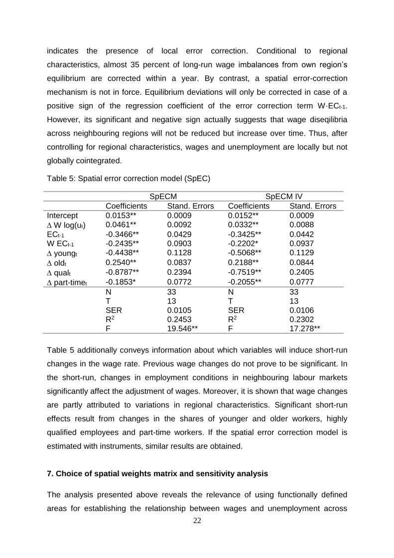
Table 5 shows the estimated regression coefficients of the local and spatial error

correction terms, ECt-1 and W·ECt-1, along with short-run changes of the explanatory

variables. Nonsignificant short-run effects on changes in wages are suppressed.

Regardless of instrumentation, the significantly negative error correction term ECt-1

22

indicates the presence of local error correction. Conditional to regional

characteristics, almost 35 percent of long-run wage imbalances from own region’s

equilibrium are corrected within a year. By contrast, a spatial error-correction

mechanism is not in force. Equilibrium deviations will only be corrected in case of a

positive sign of the regression coefficient of the error correction term W·ECt-1.

However, its significant and negative sign actually suggests that wage diseqilibria

across neighbouring regions will not be reduced but increase over time. Thus, after

controlling for regional characteristics, wages and unemployment are locally but not

globally cointegrated.

Table 5: Spatial error correction model (SpEC)

SpECM SpECM IV

Coefficients Stand. Errors Coefficients Stand. Errors

Intercept 0.0153** 0.0009 0.0152** 0.0009

W log(ut) 0.0461** 0.0092 0.0332** 0.0088

ECt-1 -0.3466** 0.0429 -0.3425** 0.0442 W ECt-1 -0.2435** 0.0903 -0.2202* 0.0937

youngt -0.4438** 0.1128 -0.5068** 0.1129

oldt 0.2540** 0.0837 0.2188** 0.0844

qualt -0.8787** 0.2394 -0.7519** 0.2405

part-timet -0.1853* 0.0772 -0.2055** 0.0777

N 33 N 33 T 13 T 13 SER 0.0105 SER 0.0106 R2 0.2453 R2 0.2302 F 19.546** F 17.278**

Table 5 additionally conveys information about which variables will induce short-run

changes in the wage rate. Previous wage changes do not prove to be significant. In

the short-run, changes in employment conditions in neighbouring labour markets

significantly affect the adjustment of wages. Moreover, it is shown that wage changes

are partly attributed to variations in regional characteristics. Significant short-run

effects result from changes in the shares of younger and older workers, highly

qualified employees and part-time workers. If the spatial error correction model is

estimated with instruments, similar results are obtained.

7. Choice of spatial weights matrix and sensitivity analysis

The analysis presented above reveals the relevance of using functionally defined

areas for establishing the relationship between wages and unemployment across

23

space. With purely administrative regions, no wage curve can be detected for East

Germany. Spatial effects are identified by adopting the contiguity approach for labour

market regions. As a simulation study of Stakhovych and Bijmolt (2008) suggests, the

choice of the spatial weights matrix may particularly affect the probability of a

recovery of the ‘true’ model and the accuracy of the estimated regression

coefficients. While the effects on the accuracy is found to be not very sensitive to the

type of weights matrix for low spatial parameter values, they are much more sensitive

for higher values. This seems in contrast to LeSage and Pace (2014) who find little

theoretical support for marked differences in inference. However, LeSage and Pace

(2014) do not rule out the possibility that different matrix choices have an impact on

the results (see also Wang, Kockelman and Wang 2013).

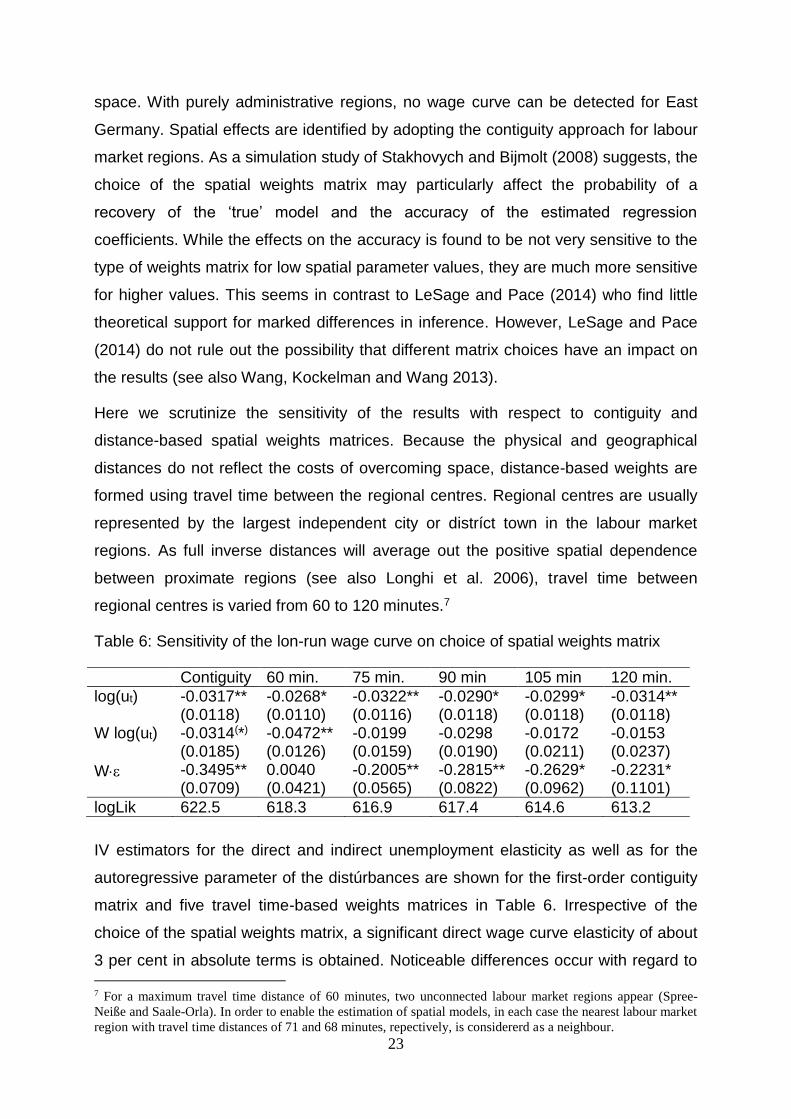
Here we scrutinize the sensitivity of the results with respect to contiguity and

distance-based spatial weights matrices. Because the physical and geographical

distances do not reflect the costs of overcoming space, distance-based weights are

formed using travel time between the regional centres. Regional centres are usually

represented by the largest independent city or distríct town in the labour market

regions. As full inverse distances will average out the positive spatial dependence

between proximate regions (see also Longhi et al. 2006), travel time between

regional centres is varied from 60 to 120 minutes.7

Table 6: Sensitivity of the lon-run wage curve on choice of spatial weights matrix

Contiguity 60 min. 75 min. 90 min 105 min 120 min.

log(ut) -0.0317** (0.0118)

-0.0268* (0.0110)

-0.0322** (0.0116)

-0.0290* (0.0118)

-0.0299* (0.0118)

-0.0314** (0.0118)

W log(ut) -0.0314(*) (0.0185)

-0.0472** (0.0126)

-0.0199 (0.0159)

-0.0298 (0.0190)

-0.0172 (0.0211)

-0.0153 (0.0237)

W -0.3495** (0.0709)

0.0040 (0.0421)

-0.2005** (0.0565)

-0.2815** (0.0822)

-0.2629* (0.0962)

-0.2231* (0.1101)

logLik 622.5 618.3 616.9 617.4 614.6 613.2

IV estimators for the direct and indirect unemployment elasticity as well as for the

autoregressive parameter of the distúrbances are shown for the first-order contiguity

matrix and five travel time-based weights matrices in Table 6. Irrespective of the

choice of the spatial weights matrix, a significant direct wage curve elasticity of about

3 per cent in absolute terms is obtained. Noticeable differences occur with regard to

7 For a maximum travel time distance of 60 minutes, two unconnected labour market regions appear (Spree-

Neiße and Saale-Orla). In order to enable the estimation of spatial models, in each case the nearest labour market

region with travel time distances of 71 and 68 minutes, repectively, is considererd as a neighbour.

24

the spillover elasticity. While the negative sign is confirmed, unemployment spillovers

appear to be significant with a threshold of 60 minutes, but nonsignificant for longer

travel times. The autoregressive coefficient of the disturbances is highly significant,

except of the shortest-distance spatial weights matrices.

Stakhovych and Bijmolt (2008) suggest selecting the correct specification on the

basis of log likelihood or information criteria. Because of the same number of

variables in all models, the log likelihood statistic is applied. According to this

criterium the contiguity approach clearly outperforms the distance approach.

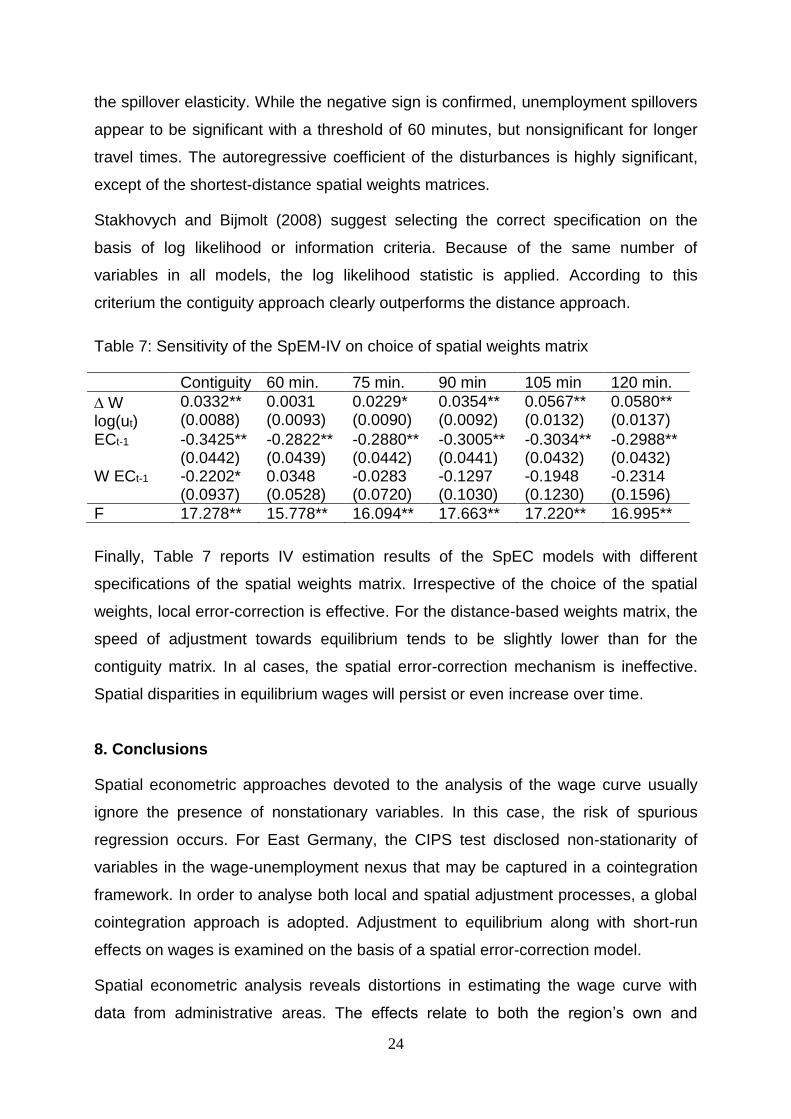
Table 7: Sensitivity of the SpEM-IV on choice of spatial weights matrix

Contiguity 60 min. 75 min. 90 min 105 min 120 min.

W log(ut)

0.0332** (0.0088)

0.0031 (0.0093)

0.0229* (0.0090)

0.0354** (0.0092)

0.0567** (0.0132)

0.0580** (0.0137)

ECt-1 -0.3425** (0.0442)

-0.2822** (0.0439)

-0.2880** (0.0442)

-0.3005** (0.0441)

-0.3034** (0.0432)

-0.2988** (0.0432)

W ECt-1 -0.2202* (0.0937)

0.0348 (0.0528)

-0.0283 (0.0720)

-0.1297 (0.1030)

-0.1948 (0.1230)

-0.2314 (0.1596)

F 17.278** 15.778** 16.094** 17.663** 17.220** 16.995**

Finally, Table 7 reports IV estimation results of the SpEC models with different

specifications of the spatial weights matrix. Irrespective of the choice of the spatial

weights, local error-correction is effective. For the distance-based weights matrix, the

speed of adjustment towards equilibrium tends to be slightly lower than for the

contiguity matrix. In al cases, the spatial error-correction mechanism is ineffective.

Spatial disparities in equilibrium wages will persist or even increase over time.

8. Conclusions

Spatial econometric approaches devoted to the analysis of the wage curve usually

ignore the presence of nonstationary variables. In this case, the risk of spurious

regression occurs. For East Germany, the CIPS test disclosed non-stationarity of

variables in the wage-unemployment nexus that may be captured in a cointegration

framework. In order to analyse both local and spatial adjustment processes, a global

cointegration approach is adopted. Adjustment to equilibrium along with short-run

effects on wages is examined on the basis of a spatial error-correction model.

Spatial econometric analysis reveals distortions in estimating the wage curve with

data from administrative areas. The effects relate to both the region’s own and

25

spillover unemployment elasticity. While no East German wage curve can be

substantiated with data for administrative districts, its existence is clearly proved for

functional labour market regions.

With a view to the theory of monosonistic competition, the long-run relationship

between wages and unemployment is analysed in a fixed-effects model that includes

the spatialy lagged unemployment rate (FE-SLX model). The relationship is

controlled for effects of work experience, qualification, gender, working time, sectoral

composition and firm size. A spatial error process is introduced to capture potential

influences of other spatilally autocorrelated variables (FE-SLX-SEM model). In order

to account for potential endogeneity, the unemployment rate is instrumented.

Applying instrument estimation methods does not substantially affect the estimate of

the region’s own wage curve elasticity, but the estimate of the spillover elasticity. The

highly significant direct uemployment elasticity of 3 per cent corroborates the

existence of a wage curve across East German labour markets. While earlier studies

report a stronger responsiveness of wages to local labour market conditons, this

estimate is well in line with the finding of Elhorst, Blien and Wolf (2007). In

instrumenting the unemployment rate, a weak significant spillover elasticity of roughly

the same size is inferred. The lower significance reflects the greater variability of

spatial externalities. Up to now, there is still a lack of knowledge on the importance of

unemployment spillovers in East Germany.

On the basis of a spatial error-correction model it is revealed that wages und the

unemployment rate are locally but not globally cointegrated. While the error-

correction mechanism works within East German labour market regions, it is not

effective between the functional areas. In contrast to the West German experience

(see Kosfeld and Dreger 2017), a spatial adjustment to equilibrium does not take

place across East German regions. A sensitivity analysis shows the robustness of the

findings with respect to contiguity- and distance-based spatial weights matrices.

Further research should pursue the cointegration approach to investigate the

heterogeneity in wage curve effects and the error-correction mechanism with respect

to different groups of workers and types of regions.

From a policy point of view, the finding of a local error-correction mechanism in

conjunction with increasing disparities in wages across East German regions

demands attention. In Germany, a discussion on the appropriate design of a system

26

for promoting less developed regions and areas with particular structural problems

from 2020 onwards has evolved. At present the common task "Improvement of

regional economic structure" (GRW) mainly ensures the scattergun approach of

comprehensive supporting East German regions. Policymakers must be aware that

untargeted subsidies bear the danger of further increasing regional disparities. As a

consequence, regional development policies should not continue to distribute

subsidies to East German regions in a non-selective way. Instead, the focus should

lie on growth poles and clusters in backward regions (s. a. Kubis, Titzes and Ragnitz

2007).

Actually, some East German regions are even more prosperous than a number of old

industrial West German regions. Therefore, the East/West divide of subsidy policy

has become overtaken. In view of this development, regional policy should focus

promotion to lagging regions and areas with structural problems in both parts of the

country.

References

Ammermüller, A., Lucifora, C., Origo, F., Zwick, T. (2012), Wage Flexibility in Regional Labour Markets: Evidence from Italy and Germany, Regional Studies 44, 401–421.

Anselin, L. (1988), Spatial Econometrics: Methods and Models, Springer, Dordrecht.

Baltagi, B. H., Baskaya, Y. S., Hulagu, T. (2012), The Turkish wage curve: Evidence from the household labor force survey. Economics Letters 114, 128-131.

Baltagi, B. H., Blien, U. (1998), The German wage curve: Evidence from the IAB employment sample, Economics Letters 61, 135-142.

Baltagi, B.H., Blien, U., Wolf, K. (2009), New evidence on the dynamic wage curve for Western Germany: 1980-2004, Labour Economics 16, 47-51.

Baltagi, B.H., Blien, U., Wolf, K. (2012), A dynamic spatial panel data approach to the German wage curve, Economic Modelling 29, 12-21.

Beenstock, M., Felsenstein, D. (2010), Spatial error correction and cointegration in nonstationary panel data: regional house prices in Israel, Journal of Geographical Systems 12, 189-206.

Beenstock, M., Felsenstein, D. (2015), Estimating spatial spillover in housing construction with nonstationary panel data, Journal of Housing Economics 28, 42-58.

Blanchflower, D. G., Oswald, A. J. (1990), The wage curve, Scandinavian Journal of Economics 92, 215-235.

Blanchflower, D. G., Oswald, A. J. (1994), The wage curve, MIT Press, Cambridge and London.

27

Blanchflower, D. G., Oswald, A. J. (1995), An Introduction to the Wage Curve, Journal of Economic Perspectives 9, 153-167.

Blanchflower, D. G., Oswald, A. J. (2005), The Wage Curve Reloaded, NBER Working Paper No. 11338

Campbell, C., Orszag, J.M. (1998), A Model of the Wage Curve, Economic Letters 59, 119-125.

Card, D. (1995), The Wage Curve: A Review, Journal of Economic Literature 33, 785-799.

Elhorst, J. P., Blien, U., Wolf, K. (2007), New evidence on the wage curve: A spatial panel approach. International Regional Science Review 30, 173-191.

Elhorst J.P. (2010), Spatial Panel Data Models, in: Fischer, M.M., Getis A. (eds.), Handbook of Applied Spatial Analysis. Springer, Berlin, Heidelberg, Germany, 377-407.

Elhorst, J.P. (2014), Spatial Econometrics - From Cross-Sectional Data to Spatial Panels, Springer, Heidelberg, Germany.

Fingleton, B., Palombi, S. (2013), The Wage Curve Reconsidered: Is it Truly an ‘Empirical Law of Economics’?, Région et développement 38, 49-92.

Fitzenberger, B., Kohn, K., Lembcke, A. (2013), Union Density and Varieties of Coverage: The Anatomy of Union Wage Effects in Germany. Industrial and Labor Relations Review 66, 169-197.

García-Mainar, I., Montuenga-Gómez,V.M. (2012), Wage dynamics in Spain: evidence from individual data (1994–2001 Investigaciones Regionales 24, 41–56:

Greene, W.H. (2011), Econometric analysis, 7th ed., Prentice Hall, Upper Saddle River, New Jersey.

Hagen, T. (2003), Three Approaches to the Evaluation of Active Labour Market Policy in East Germany Using Regional Data, Centre for European Economic Research (ZEW), Discussion Paper No. 03-27, Mannheim, Germany.

Harris, J., Todaro, M. (1970), Migration, Unemployment and Development: A Two-Sector Analysis, American Economic Review 60, 126-142.

Hilbert, C. (2008), Unemployment, wages, and the impact of active labour market policies in a regional perspective, Logos, Berlin

Im, K.S., Pesaran, M.H., Shin, Y. (2003), Testing for unit roots in heterogeneous panels. Journal of Econometrics 115, 53–74.

Kosfeld, R., Dreger, C. (2017), Local and Spatial Cointegration in the Wage Curve – A Spatial Panel Analysis of West German Regions, Review of Regional Research, Online First, 1-23.

Kosfeld, R., Werner, A. (2012), Deutsche Arbeitsmarktregionen – Neuabgrenzung nach den Kreisgebietsreformen 2007–2011, Raumforschung und Raumordnung 70, 49–64.

Kropp, P., Schwengler, B. (2016), Three-step method for delineating functional labour market regions. Regional Studies 50, 429-445.

28

Kubis, A., Titze, M., Ragnitz, J (2007), Spillover Effects of Spatial Growth Poles - a Reconciliation of Conflicting Policy Targets?, IWH-Discussion Papers, No. 8/2007, Halle (Saale), Germany.

LeSage, J.P., Pace, R.K. (2009), Introduction to Spatial Econometrics, Chapman & Hall/CRC, Boca Raton, FL.

LeSage, J.P., Pace, R.K. (2010), Spatial Econometric Models, in: Fischer, M.M., Getis, A. (eds.), Handbook of Applied Spatial Analysis – Software Tools, Methods and Applications, Springer, Berlin, Heidelberg, pp. 355-376.

LeSage, J.P., Pace, R.K. (2014), The biggest myth in spatial econometrics. Econometrics 2, 217-249.

Longhi S., Nijkamp P., Poot J. (2006), Spatial Heterogeneity and the Wage Curve Revisited, Journal of Regional Science 46, 707-731.

Mitze, T., Özyurt, S. (2014), The Spatial Dimension of Trade- and FDI-driven Productivity Growth in Chinese Provinces: A Global Cointegration Approach, Growth and Change 45, 263-291.

Moulton, B.R. (1990), An Illustration of a Pitfall in Estimating the Effects of Aggregate Variables on Micro Units, Review of Economics and Statistics 72, 334-338.

Nijkamp, P., Poot, J. (2005), The Last Word on the Wage Curve? A Meta-Analytic Assessment, Journal of Economic Surveys 19, 421-450.

Pannenberg, M., Schwarze, J. (1998), Labor market slack and the wage curve, Economics Letters 58, 351–354.

Pannenberg, M., Schwarze, J. (2000), ‘Phillips Curve’ or ‘Wage Curve’: Is there really a puzzle? Evidence for West Germany, Labour 14, 645-655.

Pesaran, M.H. (2007), A Simple Panel Unit Root Test in the Presence of Cross-Section Dependence, Journal of Applied Econometrics 22, 265-312.

Ramos, A., Nicodemo, C., Sanmorá, E. (2014), A spatial panel wage curve for Spain, Letters in Spatial and Resource Sciences 8, 125-139.

Seifert, H., Massa-Wirth, H. (2005), Pacts for employment and competitiveness in Germany, Industrial Relations Journal 36, 217–240.

Shapiro, C., Stiglitz, J.E. (1984), Equilibrium Unemployment as a Worker Discipline Device, American Economic Review 74, 433-444.

Schnabel, Claus (2016), United, Yet Apart? A Note on Persistent Labour Market Differences Between Western and Eastern Germany, Jahrbücher für Nationalökonomie und Statistik/Journal of Economics and Statistics 236, 157-180.

Stakhovych, S., Bijmolt, T.H.A. (2008), Specification of spatial models: A simulation study on weights matrices, Papers in Regional Science 88, 389-409.

Topel, R.H. (1986), Local labor markets, Journal of Political Economy 94, Supplement, 111-143.

Wagner, J. (1994), German wage curves 1979–1990. Economics Letters 44, 307–311.

Wang, Y., Kockelman, K.M., Wang, X.C. (2013), The impact of weight matrices on parameter estimation and inference: A case study of binary response using land-use data, Journal of Transport and Land Use 6, 75-85.