1

Joint Design of Radar Waveform and Detector

via End-to-end Learning with Waveform

Constraints

Wei Jiang, Student Member, IEEE, Alexander M. Haimovich, Fellow, IEEE and

Osvaldo Simeone, Fellow, IEEE

Abstract

The problem of data-driven joint design of transmitted waveform and detector in a radar system

is addressed in this paper. We propose two novel learning-based approaches to waveform and detector

design based on end-to-end training of the radar system. The first approach consists of alternating

supervised training of the detector for a fixed waveform and reinforcement learning of the transmitter for

a fixed detector. In the second approach, the transmitter and detector are trained simultaneously. Various

operational waveform constraints, such as peak-to-average-power ratio (PAR) and spectral compatibility,

are incorporated into the design. Unlike traditional radar design methods that rely on rigid mathematical

models with limited applicability, it is shown that radar learning can be robustified by training the

detector with synthetic data generated from multiple statistical models of the environment. Theoretical

considerations and results show that the proposed methods are capable of adapting the transmitted

waveform to environmental conditions while satisfying design constraints.

Index Terms

Waveform design, radar detector design, waveform constraints, reinforcement learning, supervised

learning.

W. Jiang and A. M. Haimovich are with the Center for Wireless Information Processing (CWiP), Department of Elec-trical and Computer Engineering, New Jersey Institute of Technology, Newark, NJ 07102 USA (e-mail: wj34@njit.edu;haimovich@njit.edu).

Osvaldo Simeone is with the King’s Communications, Information Processing & Learning (KCLIP) Lab, Department ofEngineering, King’s College London, London WC2R 2LS, UK (e-mail: osvaldo. simeone@kcl.ac.uk). His work was supportedby the European Research Council (ERC) under the European Union’s Horizon 2020 Research and Innovation Programme (GrantAgreement No. 725731).

arX

iv:2

102.

0969

4v1

[ee

ss.S

P] 1

9 Fe

b 20

21

2

I. INTRODUCTION

A. Context and Motivation

Design of radar waveforms and detectors has been a topic of great interest to the radar

community (see e.g. [1]-[4]). For best performance, radar waveforms and detectors should be

designed jointly [5], [6]. Traditional joint design of waveforms and detectors typically relies on

mathematical models of the environment, including targets, clutter, and noise. In contrast, this

paper proposes data-driven approaches based on end-to-end learning of radar systems, in which

reliance on rigid mathematical models of targets, clutter and noise is relaxed.

Optimal detection in the Neyman-Pearon (NP) sense guarantees highest probability of detection

for a specified probability of false alarm [1]. The NP detection test relies on the likelihood (or

log-likelihood) ratio, which is the ratio of probability density functions (PDF) of the received

signal conditioned on the presence or absence of a target. Mathematical tractability of models

of the radar environment plays an important role in determining the ease of implementation of

an optimal detector. For some target, clutter and noise models, the structure of optimal detectors

is well known [7]-[9]. For example, closed-form expressions of the NP test metric are available

when the applicable models are Gaussian [9], and, in some cases, even for non-Gaussian models

[10].

However, in most cases involving non-Gaussian models, the structure of optimal detectors

generally involves intractable numerical integrations, making the implementation of such detec-

tors computationally intensive [11], [12]. For instance, it is shown in [11] that the NP detector

requires a numerical integration with respect to the texture variable of the K-distributed clutter,

thus precluding a closed-form solution. Furthermore, detectors designed based on a specific

mathematical model of environment suffer performance degradation when the actual environment

differs from the assumed model [13], [14]. Attempts to robustify performance by designing

optimal detectors based on mixtures of random variables quickly run aground due to mathematical

intractability.

Alongside optimal detectors, optimal radar waveforms may also be designed based on the NP

criterion. Solutions are known for some simple target, clutter and noise models (see e.g. [2],

[4]). However, in most cases, waveform design based on direct application of the NP criterion

is intractable, leading to various suboptimal approaches. For example, mutual information, J-

divergence and Bhattacharyya distance have been studied as objective functions for waveform

3

design in multistatic settings [15]-[18].

In addition to target, clutter and noise models, waveform design may have to account for

various operational constraints. For example, transmitter efficiency may be improved by con-

straining the peak-to-average-power ratio (PAR) [19]-[22]. A different constraint relates to the

requirement of coexistence of radar and communication systems in overlapping spectral regions.

The National Telecommunications and Information Administration (NTIA) and Federal Com-

munication Commission (FCC) have allowed sharing of some of the radar frequency bands with

commercial communication systems [23]. In order to protect the communication systems from

radar interference, radar waveforms should be designed subject to specified compatibility con-

straints. The design of radar waveforms constrained to share the spectrum with communications

systems has recently developed into an active area of research with a growing body of literature

[24]-[28].

Machine learning has been successfully applied to solve problems for which mathematical

models are unavailable or too complex to yield optimal solutions, in domains such as computer

vision [29], [30] and natural language processing [31], [32]. Recently, a machine learning

approach has been proposed for implementing the physical layer of communication systems.

Notably, in [33], it is proposed to jointly design the transmitter and receiver of communication

systems via end-to-end learning. Reference [35] proposes an end-to-end learning-based approach

for jointly minimizing PAR and bit error rate in orthogonal frequency division multiplexing

systems. This approach requires the availability of a known channel model. For the case of

an unknown channel model, reference [36] proposes an alternating training approach, whereby

the transmitter is trained via reinforcement learning (RL) on the basis of noiseless feedback

from the receiver, while the receiver is trained by supervised learning. In [37], the authors

apply simultaneous perturbation stochastic optimization for approximating the gradient of a

transmitter’s loss function. A detailed review of the state of the art can be found in [38] (see

also [39]-[41] for recent work).

In the radar field, learning machines trained in a supervised manner based on a suitable loss

function have been shown to approximate the performance of the NP detector [42], [43]. As

a representative example, in [43], a neural network trained in a supervised manner using data

that includes Gaussian interference, has been shown to approximate the performance of the NP

detector. Note that design of the NP detector requires express knowledge of the Gaussian nature

of the interference, while the neural network is trained with data that happens to be Gaussian,

4

but the machine has no prior knowledge of the statistical nature of the data.

B. Main contributions

In this work, we introduce two learning-based approaches for the joint design of waveform and

detector in a radar system. Inspired by [36], end-to-end learning of a radar system is implemented

by alternating supervised learning of the detector for a fixed waveform, and RL-based learning

of the transmitter for a fixed detector. In the second approach, the learning of the detector and

waveform are executed simultaneously, potentially speeding up training in terms of required radar

transmissions to yield the training samples compared alternating training. In addition, we extend

the problem formulation to include training of waveforms with PAR or spectral compatibility

constraints.

The main contributions of this paper are summarized as follows:

1) We formulate a radar system architecture based on the training of the detector and the

transmitted waveform, both implemented as feedforward multi-layer neural networks.

2) We develop two end-to-end learning algorithms for detection and waveform generation. In

the first learning algorithm, detector and transmitted waveform are trained alternately: For

a fixed waveform, the detector is trained using supervised learning so as to approximate the

NP detector; and for a fixed detector, the transmitted waveform is trained via policy gradient-

based RL. In the second algorithm, the detector and transmitter are trained simultaneously.

3) We extend learning algorithms to incorporate waveform constraints, specifically PAR and

spectral compatibility constraints.

4) We provide theoretical results that relate alternating and simultaneous training by computing

the gradients of the loss functions optimized by both methods.

5) We also provide theoretical results that justify the use of RL-based transmitter training by

comparing the gradient used by this procedure with the gradient of the ideal model-based

likelihood function.

This work extends previous results presented in the conference version [44]. In particular,

reference [44] proposes a learning algorithm, whereby supervised training of the radar detector

is alternated with RL-based training of the unconstrained transmitted waveforms. As compared to

the conference version [44], this paper studies also a simultaneous training; it develops methods

for learning radar waveforms with various operational waveform constraints; and it provides

5

a theoretical results regarding the relationship between alternating training and simultaneous

training, as well as regarding the adoption of RL-based training of the transmitter.

The rest of this paper is organized as follows. A detailed system description of the end-to-end

radar system is presented in Section II. Section III proposes two iterative algorithms of jointly

training the transmitter and receiver. Section IV provides theoretical properties of gradients

Numerical results are reported in Section V. Finally, conclusions are drawn in Section VI.

Throughout the paper bold lowercase and uppercase letters represent vector and matrix,

respectively. The conjugate, the transpose, and the conjugate transpose operator are denoted

by the symbols (·)∗, (·)T , and (·)H , respectively. The notations CK and RK represent sets of

K-dimensional vectors of complex and real numbers, respectively. The notation | · | indicates

modulus, || · || indicates the Euclidean norm, and Ex∼px· indicates the expectation of the

argument with respect to the distribution of the random variable x ∼ px, respectively. <(·) and

=(·) stand for real-part and imaginary-part of the complex-valued argument, respectively. The

letter j represents the imaginary unit, i.e., j =√−1. The gradient of a function f : Rn → Rm

with respect to x ∈ Rn is ∇xf(x) ∈ Rn×m.

II. PROBLEM FORMULATION

Consider a pulse-compression radar system that uses the baseband transmit signal

x(t) =K∑k=1

ykζ(t− [k − 1]Tc

), (1)

where ζ(t) is a fixed basic chip pulse, Tc is the chip duration, and ykKk=1 are complex

deterministic coefficients. The vector y , [y1, . . . , yK ]T is referred to as the fast-time waveform

of the radar system, and is subject to design.

The backscattered baseband signal from a stationary point-like target is given by

z(t) = αx(t− τ) + c(t) + n(t), (2)

where α is the target complex-valued gain, accounting for target backscattering and channel

propagation effects; τ represents the target delay, which is assumed to satisfy the target de-

tectability condition condition τ >> KTc; c(t) is the clutter component; and n(t) denotes signal-

independent noise comprising an aggregate of thermal noise, interference, and jamming. The

6

clutter component c(t) associated with a detection test performed at τ = 0 may be expressed

c(t) =K−1∑

g=−K+1

γgx(t− gTc

), (3)

where γg is the complex clutter scattering coefficient at time delay τ = 0 associated with the

gth range cell relative to the cell under test. Following chip matched filtering with ζ∗(−t), and

sampling at Tc−spaced time instants t = τ + [k − 1]Tc for k ∈ 1, . . . K, the K × 1 discrete-

time received signal z = [z(τ), z(τ + Tc), . . . , z(τ + [K − 1]Tc)]T for the range cell under test

containing a point target with complex amplitude α, clutter and noise can be written as

z = αy + c + n, (4)

where c and n denote, respectively, the clutter and noise vectors.

Detection of the presence of a target in the range cell under test is formulated as the following

binary hypothesis testing problem: H0 : z = c + n

H1 : z = αy + c + n.(5)

In traditional radar design, the golden standard for detection is provided by the NP criterion of

maximizing the probability of detection for a given probability of false alarm. Application of

the NP criterion leads to the likelihood ratio test

Λ(z) =p(z|y,H1)

p(z|y,H0)

H1

≷H0

TΛ, (6)

where Λ(z) is the likelihood ratio, and TΛ is the detection threshold set based on the probability

of false alarm constraint [5]. The NP criterion is also the golden standard for designing a radar

waveform that adapts to the given environment, although, as discussed earlier, a direct application

of this design principle is often intractable.

The design of optimal detectors and/or waveforms under the NP criterion requires on channel

models of the radar environment, namely, knowledge of the conditional probabilities p(z|y,Hi)

for i = 0, 1. The channel model p(z|y,Hi) is the likelihood of the observation z conditioned

on the transmitted waveform y and hypothesis Hi. In the following, we introduce an end-to-end

radar system in which the detector and waveform are jointly learned in a data-driven fashion.

7

Transmitter Receiver

Radar operating environment

Detector

Fig. 1. An end-to-end radar system operating over an unknown radar operating environment. Transmitter and receiver areimplemented as two separate parametric functions fθT (·) and fθR(·) with trainable parameter vectors θT and θR, respectively.

A. End-to-end radar system

The end-to-end radar system illustrated in Fig. 1 comprises a transmitter and a receiver that

seek to detect the presence of a target. Transmitter and receiver are implemented as two separate

parametric functions fθT(·) and fθR

(·) with trainable parameter vectors θT and θR, respectively.

As shown in Fig. 1, the input to the transmitter is a user-defined initialization waveform

s ∈ CK . The transmitter outputs a radar waveform obtained through a trainable mapping yθT=

fθT(s) ∈ CK . The environment is modeled as a stochastic system that produces the vector

z ∈ CK from a conditional PDF p(z|yθT,Hi) parameterized by a binary variable i ∈ 0, 1.

The absence or presence of a target is indicated by the values i = 0 and i = 1 respectively,

and hence i is referred to as the target state indicator. The receiver passes the received vector z

through a trainable mapping p = fθR(z), which produces the scalar p ∈ (0, 1). The final decision

i ∈ 0, 1 is made by comparing the output of the receiver p to a hard threshold in the interval

(0, 1).

B. Transmitter and Receiver Architectures

As discussed in Section II-A, the transmitter and the receiver are implemented as two separate

parametric functions fθT(·) and fθR

(·). We now detail an implementation of the transmitter fθT(·)

and receiver fθR(·) based on feedforward neural networks.

A feedforward neural network is a parametric function fθ(·) that maps an input real-valued

vector uin ∈ RNin to an output real-valued vector uout ∈ RNout via L successive layers, where Nin

and Nout represent, respectively, the number of neurons of the input and output layers. Noting

that the input to the lth layer is the output of the (l − 1)th layer, the output of the lth layer is

8

given by

ul = fθ[l](ul−1) = φ(W[l]ul−1 + b[l]

), for l = 1, . . . , L, (7)

where φ(·) is an element-wise activation function, and θ[l] = W[l],b[l] contains the train-

able parameter of the lth layer comprising the weight W[l] and bias b[l]. The vector of train-

able parameters of the entire neural network comprises the parameters of all layers, i.e., θ =

vecθ[1], · · · ,θ[L].

The architecture of the end-to-end radar system with transmitter and receiver implemented

based on feedforward neural networks is shown in Fig. 2. The transmitter applies a complex

initialization waveform s to the function fθT(·). The complex-value input s is processed by a

complex-to-real conversion layer. This is followed by a real-valued neural network fθT(·). The

output of the neural network is converted back to complex-values, and an output layer normalizes

the transmitted power. As a result, the transmitter generates the radar waveform yθT.

The receiver applies the received signal z to the function fθR(·). Similar to the transmitter, a

first layer converts complex-valued to real-valued vectors. The neural network at the receiver is

denoted fθR(·). The task of the receiver is to generate a scalar p ∈ (0, 1) that approximates the

posterior probability of the presence of a target conditioned on the received vector z. To this end,

the last layer of the neural network fθR(·) is selected as a logistic regression layer consisting of

operating over a linear combination of outputs from the previous layer. The presence or absence

of the target is determined based on the output of the receiver and a threshold set according to

a false alarm constraint.

III. TRAINING OF END-TO-END RADAR SYSTEMS

This section discusses the joint optimization of the trainable parameter vectors θT and θR

to meet application-specific performance requirements. Two training algorithms are proposed to

train the end-to-end radar system. The first algorithm alternates between training of the receiver

and of the transmitter. This algorithm is referred to as alternating training, and is inspired by

the approach used in [36] to train encoder and decoder of a digital communication system. In

contrast, the second algorithm trains the receiver and transmitter simultaneously. This approach is

referred to as simultaneous training. Note that the proposed two training algorithms are applicable

to other differentiable parametric functions implementing the transmitter fθT(·) and the receiver

9

Radar operating environment

Neural network

Normalization layer

Neural network

Receiver

Transmitter

Fig. 2. Transmitter and receiver architectures based on feedforward neural networks.

fθR(·), such as recurrent neural network or its variants [45]. In the following, we first discuss

alternating training and then we detail simultaneous training.

A. Alternating Training: Receiver Design

Alternating training consists of iterations encompassing separate receiver and transmitter up-

dates. In this subsection, we focus on the receiver updates. A receiver training update optimizes

the receiver parameter vector θR for a fixed transmitter waveform yθT. Receiver design is

supervised in the sense that we assume the target state indicator i to be available to the receiver

during training. Supervised training of the receiver for a fixed transmitter’s parameter vector θT

is illustrated in Fig. 3.

Receivertraining

Fig. 3. Supervised training of the receiver for a fixed transmitted waveform.

The standard cross-entropy loss [43] is adopted as the loss function for the receiver. For a

given transmitted waveform yθT= fθT

(s), the receiver average loss function is accordingly

10

given byLR(θR) =

∑i∈0,1

P (Hi)Ez∼p(z|yθT,Hi)

`(fθR

(z), i), (8)

where P (Hi) is the prior probability of the target state indicator i, and `(fθR

(z), i)

is the

instantaneous cross-entropy loss for a pair(fθR

(z), i), namely,

`(fθR

(z), i)

= −i ln fθR(z)− (1− i) ln

[1− fθR

(z)]. (9)

For a fixed transmitted waveform, the receiver parameter vector θR should be ideally optimized

by minimizing (8), e.g., via gradient descent or one of its variants [46]. The gradient of average

loss (8) with respect to the receiver parameter vector θR is

∇θRLR(θR) =

∑i∈0,1

P (Hi)Ez∼p(z|yθT,Hi)

∇θR

`(fθR

(z), i). (10)

This being a data-driven approach, rather than assuming known prior probability of the target

state indicator P (Hi) and likelihood p(z|yθT,Hi), the receiver is assumed to have access to

QR independent and identically distributed (i.i.d.) samples DR =z(q) ∼ p(z|yθT

,Hi(q)), i(q) ∈

0, 1QR

q=1.

Given the output of the receiver function fθR(z(q)) for a received sample vector z(q) and

the indicator i(q) ∈ 0, 1, the instantaneous cross-entropy loss is computed from (9), and the

estimated receiver gradient is given by

∇θRLR(θR) =

1

QR

QR∑q=1

∇θR`(fθR

(z(q)), i(q)). (11)

Using (11), the receiver parameter vector θR is adjusted according to stochastic gradient descent

updates

θ(n+1)R = θ

(n)R − ε∇θR

LR(θ(n)R ) (12)

across iterations n = 1, 2, · · · , where ε > 0 is the learning rate.

B. Alternating Training: Transmitter Design

In the transmitter training phase of alternating training, the receiver parameter vector θR is

held constant, and the function fθT(·) implementing the transmitter is optimized. The goal of

11

transmitter training is to find an optimized parameter vector θT that minimizes the cross-entropy

loss function (8) seen as a function of θT .

As illustrated in Fig. 4, a stochastic transmitter outputs a waveform a drawn from a distribution

π(a|yθT) conditioned on yθT

= fθT(s). The introduction of the randomization π(a|yθT

) of the

designed waveform yθTis useful to enable exploration of the design space in a manner akin

to standard RL policies. To train the transmitter, we aim to minimize the average cross-entropy

lossLπT (θT ) =

∑i∈0,1

P (Hi)Ea∼π(a|yθT)

z∼p(z|a,Hi)

`(fθR

(z), i). (13)

Note that this is consistent with (8), with the caveat that an expectation is taken over policy

π(a|yθT). This is indicated by the superscript “π”.

Transmittertraining

Stochastic transmitter

Fig. 4. RL-based transmitter training for a fixed receiver design.

Assume that the policy π(a|yθT) is differentiable with respect to the transmitter parameter

vector θT , i.e., that the gradient ∇θTπ(a|yθT

) exists. The policy gradient theorem [47] states

that the gradient of the average loss (13) can be written as

∇θTLπT (θT ) =

∑i∈0,1

P (Hi)Ea∼π(a|yθT)

z∼p(z|a,Hi)

`(fθR

(z), i)∇θT

lnπ(a|yθT). (14)

The gradient (14) has the important advantage that it may be estimated via QT i.i.d. samples

DT =a(q) ∼ π(a|yθT

), z(q) ∼ p(z|a(q),Hi(q)), i(q) ∈ 0, 1

QT

q=1, yielding the estimate

∇θTLπT (θT ) =

1

QT

QT∑q=1

`(fθR

(z(q)), i(q))∇θT

ln π(a(q)|yθT). (15)

With estimate (15), in a manner similar to (12), the transmitter parameter vector θT may be

12

optimized iteratively according to the stochastic gradient descent update rule

θ(n+1)T = θ

(n)T − ε∇θT

LπT (θ(n)T ) (16)

over iterations n = 1, 2, · · · . The alternating training algorithm is summarized as Algorithm 1.

The training process is carried out until a stopping criterion is satisfied. For example, a prescribed

number of iterations may have been reached, or a number of iterations may have elapsed during

which the training loss (13), estimated using samples DT , may have not decreased by more than

a given amount.

Algorithm 1: Alternating TrainingInput: initialization waveform s; stochastic policy πθT

(·|y); learning rate εOutput: learned parameter vectors θR and θT

1 initialize θ(0)R and θ

(0)T , and set n = 0

2 while stopping criterion not satisfied do/* receiver training phase */

3 evaluate the receiver loss gradient ∇θRLR(θ

(n)R ) from (11) with θT = θ

(n)T

4 update receiver parameter vector θR via

θ(n+1)R = θ

(n)R − ε∇θR

LR(θ(n)R )

and stochastic transmitter policy turned off/* transmitter training phase */

5 evaluate the transmitter loss gradient ∇θTLπT (θ

(n)T ) from (15) with θR = θ

(n+1)R

6 update transmitter parameter vector θT via

θ(n+1)T = θ

(n)T − ε∇θT

LπT (θ(n)T )

7 n← n+ 18 end

C. Transmitter Design with Constraints

We extend the transmitter training discussed in the previous section to incorporate waveform

constraints on PAR and spectral compatibility. To this end, we introduce penalty functions that

are used to modify the training criterion (13) to meet these constraints.

1) PAR Constraint: Low PAR waveforms are preferred in radar systems due to hardware

limitations related to waveform generation. A lower PAR entails a lower dynamic range of the

13

power amplifier, which in turn allows an increase in average transmitted power. The PAR of a

radar waveform yθT= fθT

(s) may be expressed

JPAR(θT ) =max

k=1,··· ,K|y

θT,k|2

||yθT||2/K

, (17)

which is bounded according to 1 ≤ JPAR(θT ) ≤ K.

2) Spectral Compatibility Constraint: A spectral constraint is imposed when a radar system

is required to operate over a spectrum partially shared with other systems such as wireless

communication networks. Suppose there are D frequency bands ΓdDd=1 shared by the radar

and by the coexisting systems, where Γd = [fd,l, fd,u], with fd,l and fd,u denoting the lower and

upper normalized frequencies of the dth band, respectively. The amount of interfering energy

generated by the radar waveform yθTin the dth shared band is

∫ fd,u

fd,l

∣∣∣∣∣K−1∑k=0

yθT,ke−j2πfk

∣∣∣∣∣2

df = yHθTΩdyθT

, (18)

where [Ωd

]v,h

=

fd,u − fd,l if v = h

ej2πfd,u(v−h) − ej2πfd,l(v−h)

j2π(v − h)if v 6= h

(19)

for (v, h) ∈ 1, · · · , K2. Let Ω =∑D

d=1 ωdΩd be a weighted interference covariance matrix,

where the weights ωdDd=1 are assigned based on practical considerations regarding the impact

of interference in the D bands. These include distance between the radar transmitter and interfer-

enced systems, and tactical importance of the coexisting systems [48]. Given a radar waveform

yθT= fθT

(s), we define the spectral compatibility penalty function as

Jspectrum(θT ) = yHθTΩyθT

, (20)

which is the total interfering energy from the radar waveform produced on the shared frequency

bands.

3) Constrained Transmitter Design: For a fixed receiver parameter vector θR, the average

loss (13) is modified by introducing a penalty function J ∈ JPAR, Jspectrum. Accordingly, we

14

formulate the transmitter loss function, encompassing (13), (17) and (20), as

LπT,c(θT ) = LπT (θT ) + λJ(θT )

=∑i∈0,1

P (Hi)Ea∼π(a|yθT)

z∼p(z|a,Hi)

`(fθR

(z), i)

+ λJ(θT ).(21)

where λ controls the weight of the penalty J(θT ), and is referred to as the penalty parameter.

When the penalty parameter λ is small, the transmitter is trained to improve its ability to adapt to

the environment, while placing less emphasis on reducing the PAR level or interference energy

from the radar waveform; and vice versa for large values of λ. Note that the waveform penalty

function J(θT ) depends only on the transmitter trainable parameters θT . Thus, imposing the

waveform constraint does not affect the receiver training.

It is straightforward to write the estimated version of the gradient (21) with respect to θT by

introducing the penalty as

∇θTLπT,c(θT ) = ∇θT

LπT (θT ) + λ∇θTJ(θT ), (22)

where the gradient of the penalty function ∇θTJ(θT ) is provided in Appendix A.

Substituting (15) into (22), we finally have the estimated gradient

∇θTLπT,c(θT ) =

1

QT

QT∑q=1

`(fθR

(z(q)), i(q))∇θT

lnπ(a(q)|yθT) + λ∇θT

J(θT ), (23)

which is used in the stochastic gradient update rule

θ(n+1)T = θ

(n)T − ε∇θT

LπT,c(θ(n)T ) for n = 1, 2, · · · . (24)

D. Simultaneous Training

This subsection discusses simultaneous training, in which the receiver and transmitter are

updated simultaneously as illustrated in Fig. 5. To this end, the objective function is the average

lossLπ(θR,θT ) =

∑i∈0,1

P (Hi)Ea∼π(a|yθT)

z∼p(z|a,Hi)

`(fθR

(z), i). (25)

This function is minimized over both parameters θR and θT via stochastic gradient descent.

15

Receivertraining

Transmittertraining

Stochastic transmitter

Fig. 5. Simultaneous training of the end-to-end radar system. The receiver is trained by supervised learning, while the transmitter

is trained by RL.

The gradient of (25) with respect to θR is

∇θRLπ(θR,θT ) =

∑i∈0,1

P (Hi)Ea∼π(a|yθT)

z∼p(z|a,Hi)

∇θR

`(fθR

(z), i), (26)

and the gradient of (25) with respect to θT is

∇θTLπ(θR,θT ) =

∑i∈0,1

P (Hi)∇θTEa∼π(a|yθT

)

z∼p(z|a,Hi)

`(fθR

(z), i)

=∑i∈0,1

P (Hi)Ea∼π(a|yθT)

z∼p(z|a,Hi)

`(fθR

(z), i)∇θT

ln π(a|yθT).

(27)

To estimate gradients (26) and (27), we assume access to Q i.i.d. samples D =a(q) ∼

π(a|yθT), z(q) ∼ p(z|a(q),Hi(q)), i

(q) ∈ 0, 1Qq=1

. From (26), the estimated receiver gradient is

∇θRLπ(θR,θT ) =

1

Q

Q∑q=1

∇θR`(fθR

(z(q)), i(q)). (28)

Note that, in (28), the received vector z(q) is obtained based on a given waveform a(q) sampled

from policy π(a|yθT). Thus, the estimated receiver gradient (28) is averaged over the stochastic

waveforms a. This is in contrast to alternating training, in which the receiver gradient depends

directly on the transmitted waveform yθT.

From (27), the estimated transmitter gradient is given by

∇θTLπ(θR,θT ) =

1

Q

Q∑q=1

`(fθR

(z(q)), i(q))∇θT

ln π(a(q)|yθT). (29)

Finally, denote the parameter set θ = θR,θT, from (28) and (29), the trainable parameter set

16

θ is updated according to the stochastic gradient descent rule

θ(n+1) = θ(n) − ε∇θLπ(θ(n)R ,θ

(n)T ) (30)

across iterations n = 1, 2, · · · .

The simultaneous training algorithm is summarized in Algorithm 2. Like alternating training,

simultaneous training can be directly extended to incorporate prescribed waveform constraints

by adding the penalty term λJ(θT ) to the average loss (25).

Algorithm 2: Simultaneous TrainingInput: initialization waveform s; stochastic policy π(·|yθT

); learning rate εOutput: learned parameter vectors θR and θT

1 initialize θ(0)R and θ

(0)T , and set n = 0

2 while stopping criterion not satisfied do3 evaluate the receiver gradient ∇θR

Lπ(θ(n)R ,θ

(n)T ) and the transmitter gradient

∇θTLπ(θ

(n)R ,θ

(n)T ) from (28) and (29), respectively

4 update receiver parameter vector θR and transmitter parameter vector θTsimultaneously via

θ(n+1)R = θ

(n)R − ε∇θR

Lπ(θ(n)R ,θ

(n)T )

andθ

(n+1)T = θ

(n)T − ε∇θT

Lπ(θ(n)R ,θ

(n)T )

5 n← n+ 16 end

IV. THEORETICAL PROPERTIES OF THE GRADIENTS

In this section, we discuss two useful theoretical properties of the gradients used for learning

receiver and transmitter.

A. Receiver Gradient

As discussed previously, end-to-end learning of transmitted waveform and detector may be

accomplished either by alternating or simultaneous training. The main difference between alter-

nating and simultaneous training concerns the update of the receiver trainable parameter vector

θR. Alternating training of θR relies on a fixed waveform yθT(see Fig. 3), while simultaneous

training relies on random waveforms a generated in accordance with a preset policy, i.e.,

17

a ∼ π(a|yθT), as shown in Fig. 5. The relation between the gradient applied by alternating

training, ∇θRLR(θR), and the gradient of simultaneous training, ∇θR

Lπ(θR,θT ), with respect

to θR is stated by the following proposition.

Proposition 1. For the loss function (8) computed based on a waveform yθTand loss function

(13) computed based on a stochastic policy π(a|yθT) continuous in a, the following equality

holds:

∇θRLR(θR) = ∇θR

Lπ(θR,θT ). (31)

Proof. See Appendix B.

Proposition 1 states that the gradient of simultaneous training, ∇θRLπ(θR,θT ), equals the

gradient of alternating training, ∇θRLR(θR), even though simultaneous training applies a random

waveform a ∼ π(a|yθT) to train the receiver. Note that this result applies only to ensemble

means according to (8) and (26), and not to the empirical estimates used by Algorithms 1 and

2. Nevertheless, Proposition 1 suggests that training updates of the receiver are unaffected by

the choice of alternating or simultaneous training. That said, given the distinct updates of the

transmitter’s parameter, the overall trajectory of the parameters (θR, θT ) during training may

differ according to the two algorithms.

B. Transmitter gradient

As shown in the previous section, the gradients used for learning receiver parameters θR

by alternating training (11) or simultaneous training (28) may be directly estimated from the

channel output samples z(q). In contrast, the gradient used for learning transmitter parameters θT

according to (8) cannot be directly estimated from the channel output samples. To obviate this

problem, in Algorithms 1 and 2, the transmitter is trained by exploring the space of transmitted

waveforms according to a policy π(a|yθT). We refer to the transmitter loss gradient obtained via

policy gradient (27) as the RL transmitter gradient. The benefit of RL-based transmitter training

is that it renders unnecessary access to the likelihood function p(z|yθT,Hi) to evaluate the RL

transmitter gradient, rather the gradient is estimated via samples. We now formalize the relation

of the RL transmitter gradient (27) and the transmitter gradient for a known likelihood obtained

according to (8).

As mentioned, if the likelihood p(z|yθT,Hi) were known, and if it were differentiable with

respect to the transmitter parameter vector θT , the transmitter parameter vector θT may be

18

learned by minimizing the average loss (8), which we rewrite as a function of both θR and θT

as

L(θR,θT ) =∑i∈0,1

P (Hi)Ez∼p(z|yθT,Hi)

`(fθR

(z), i). (32)

The gradient of (32) with respect to θT is expressed as

∇θTL(θR,θT ) =

∑i∈0,1

P (Hi)Ez∼p(z|yθT,Hi)

`(fθR

(z), i)∇θT

ln p(z|yθT,Hi)

, (33)

where the equality leverages the following relation

∇θTp(z|yθT

,Hi) = p(z|yθT,Hi)∇θT

ln p(z|yθT,Hi). (34)

The relation between the RL transmitter gradient ∇θTLπ(θR,θT ) in (27) and the transmitter

gradient ∇θTL(θR,θT ) in (33) is elucidated by the following proposition.

Proposition 2. If likelihood function p(z|yθT,Hi) is differentiable with respect to the transmitter

parameter vector θT for i ∈ 0, 1, the following equality holds

∇θTLπ(θR,θT ) = ∇θT

L(θR,θT ). (35)

Proof. See Appendix C.

Proposition 2 establishes that the RL transmitter gradient ∇θTLπ(θR,θT ) equals the trans-

mitter gradient ∇θTL(θR,θT ) for any given receiver parameters θR. Proposition 2 hence pro-

vides a theoretical justification for replacing the gradient ∇θTL(θR,θT ) with the RL gradient

∇θTLπ(θR,θT ) to perform transmitter training as done in Algorithms 1 and 2.

V. NUMERICAL RESULTS

This section first introduces the simulation setup, and then it presents numerical examples of

waveform design and detection performance that compare the proposed data-driven methodology

with existing model-based approaches. While simulation results presented in this section rely

on various models of target, clutter and interference, this work expressly distinguishes data-

driven learning from model-based design. Learning schemes rely solely on data and not on

model information. In contrast, model-based design implies a system structure that is based

on a specific and known model. Furthermore, learning may rely on synthetic data containing

diverse data that is generated according to a variety of models. In contrast, model-based design

19

typically relies on a single model. For example, as we will see, a synthetic dataset for learning

may contain multiple clutter sample sets, each generated according to a different clutter model.

Conversely, a single clutter model is typically assumed for model-based design.

A. Models, Policy, and Parameters

1) Models of target, clutter, and noise: The target is stationary, and has a Rayleigh envelope,

i.e., α ∼ CN (0, σ2α). The noise has a zero-mean Gaussian distribution with the correlation matrix

[Ωn]v,h = σ2nρ|v−h| for (v, h) ∈ 1, · · · , K2, where σ2

n is the noise power and ρ is the one-lag

correlation coefficient. The clutter vector in (4) is the superposition of returns from 2K − 1

consecutive range cells, reflecting all clutter illuminated by the K-length signal as it sweeps in

range across the target. Accordingly, the clutter vector may be expressed as

c =K−1∑

g=−K+1

γgJgy, (36)

where Jg represents the shifting matrix at the gth range cell with elements

[Jg]v,h

=

1 if v − h = g

0 if v − h 6= g(v, h) ∈ 1, · · · , K2 . (37)

The magnitude |γg| of the gth clutter scattering coefficient is generated according to a Weibull

distribution [5]

p(|γg|) =β

νβ|γg|β−1 exp

(− |γg|

β

νβ

), (38)

where β is the shape parameter and ν is the scale parameter of the distribution. Let σ2γg represent

the power of the clutter scattering coefficient γg. The relation between σ2γg and the Weibull

distribution parameters β, ν is [50]

σ2γg = E|γg|2 =

2ν2

βΓ

(2

β

), (39)

where Γ(·) is the Gamma function. The nominal range of the shape parameter is 0.25 ≤ β ≤

2 [51]. In the simulation, the complex-valued clutter scattering coefficient γg is obtained by

multiplying a real-valued Weibull random variable |γg| with the factor exp(jψg), where ψg is

the phase of γg distributed uniformly in the interval (0, 2π). When the shape parameter β = 2,

the clutter scattering coefficient γg follows the Gaussian distribution γg ∼ CN (0, σ2γg). Based

on the assumed mathematical models of the target, clutter and noise, it can be shown that the

20

optimal detector in the NP sense is the square law detector [9], and the adaptive waveform

for target detection can be obtained by maximizing the signal-to-clutter-plus-noise ratio at the

receiver output at the time of target detection (see Appendix A of [44] for details).

2) Transmitter and Receiver Models: Waveform generation and detection is implemented

using feedforward neural networks as explained in Section II-B. The transmitter fθT(·) is a

feedforward neural network with four layers, i.e., an input layer with 2K neurons, two hidden

layers with M = 24 neurons, and an output layer with 2K neurons. The activation function

is exponential linear unit (ELU) [52]. The receiver fθR(·) is implemented as a feedforward

neural network with four layers, i.e., an input layer with 2K neurons, two hidden layers with M

neurons, and an output layer with one neuron. The sigmoid function is chosen as the activation

function. The layout of transmitter and receiver networks is summarized in Table I.

Table I

LAYOUT OF THE TRANSMITTER AND RECEIVER NETWORKS

Transmitter fθT (·) Receiver fθR(·)

Layer 1 2-3 4 1 2-3 4

Dimension 2K M 2K 2K M 1

Activation - ELU Linear - Sigmoid Sigmoid

3) Gaussian policy: A Gaussian policy π(a|yθT) is adopted for RL-based transmitter training.

Accordingly, the output of the stochastic transmitter follows a complex Gaussian distribution

a ∼ π(a|yθT) = CN

(√1− σ2

pyθT,σ2p

KIK), where the per-chip variance σ2

p is referred to as the

policy hyperparameter. When σ2p = 0, the stochastic policy becomes deterministic [49], i.e.,

the policy is governed by a Dirac function at yθT. In this case, the policy does not explore

the space of transmitted waveforms, but it “exploits” the current waveform. At the opposite

end, when σ2p = 1, the output of the stochastic transmitter is independent of yθT

, and the

policy becomes zero-mean complex-Gaussian noise with covariance matrix IK/K. Thus, the

policy hyperparameter σ2p is selected in the range (0, 1), and its value sets a trade-off between

exploration of new waveforms versus exploitation of current waveform.

4) Training Parameters: The initialization waveform s is a linear frequency modulated pulse

with K = 8 complex-valued chips and chirp rate R = (100×103)/(40×10−6) Hz/s. Specifically,

21

the kth chip of s is given by

s(k) =1√K

expjπR

(k/fs

)2 (40)

for ∀k ∈ 0, . . . , K − 1, where fs = 200 kHz. The signal-to-noise ratio (SNR) is defined as

SNR = 10 log10

σ2α

σ2n

. (41)

Training was performed at SNR = 12.5 dB. The clutter environment is uniform with σ2γg = −11.7

dB, ∀g ∈ −K + 1, . . . , K − 1, such that the overall clutter power is∑K−1

g=−(K−1) σ2γg = 0 dB.

The noise power is σ2n = 0 dB, and the one-lag correlation coefficient ρ = 0.7. Denote βtrain

and βtest the shape parameters of the clutter distribution (38) applied in training and test stage,

respectively. Unless stated otherwise, we set βtrain = βtest = 2.

To obtain a balanced classification dataset, the training set is populated by samples belonging

to either hypothesis with equal prior probability, i.e., P (H0) = P (H1) = 0.5. The number of

training samples is set as QR = QT = Q = 213 in the estimated gradients (11), (15), (28),

and (29). Unless stated otherwise, the policy parameter is set to σ2p = 10−1.5, and the penalty

parameter is λ = 0, i.e., there are no waveform constraints. The Adam optimizer [53] is adopted

to train the system over a number of iterations chosen by trial and error. The learning rate is

ε = 0.005. In the testing phase, 2 × 105 samples are used to estimate the probability of false

alarm (Pfa) under hypothesis H0, while 5× 104 samples are used to estimate the probability of

detection (Pd) under hypothesis H1. Receiver operating characteristic (ROC) curves are obtained

via Monte Carlo simulations by varying the threshold applied at the output of the receiver. Results

are obtained by averaging over fifty trials. Numerical results presented in this section assume

simultaneous training, unless stated otherwise.

B. Results and Discussion

1) Simultaneous Training vs Training with Known Likelihood: We first analyze the impact of

the choice of the policy hyperparameter σ2p on the performance on the training set. Fig. 6 shows

the empirical cross-entropy loss of simultaneous training versus the policy hyperparameter σ2p

upon the completion of the training process. The empirical loss of the system training with a

known channel (32) is plotted as a comparison. It is seen that there is an optimal policy parameter

σ2p for which the empirical loss of simultaneous training approaches the loss with known channel.

22

Fig. 6. Empirical training loss versus policy hyperparameter σ2p for simultaneous training algorithm and training with known

channel, respectively.

As the policy hyperparameter σ2p tends to 0, the output of the stochastic transmitter a is close

to the waveform yθT, which leads to no exploration of the space of transmitted waveforms.

In contrast, when the policy parameter σ2p tends to 1, the output of the stochastic transmitter

becomes a complex Gaussian noise with zero mean and covariance matrix IK/K. In both cases,

the RL transmitter gradient is difficult to estimate accurately.

While Fig. 6 evaluates the performance on the training set in terms of empirical cross-entropy

loss, the choice of the policy hyperparameter σ2p should be based on validation data and in

terms of the testing criterion that is ultimately of interest. To elaborate on this point, ROC

curves obtained by simultaneous training with different values of the policy hyperparameter σ2p

and training with known channel are shown in Fig. 7. As shown in the figure, simultaneous

training with σ2p = 10−1.5 achieves a similar ROC as training with known channel. The choice

σ2p = 10−1.5, also has the lowest empirical training loss in Fig. 6. These results suggest that

training is not subject to overfitting [34].

2) Simultaneous Training vs Alternating Training: We now compare simultaneous and alter-

nating training in terms of ROC curves in Fig. 8. ROC curves based on the optimal detector in

the NP sense, namely, the square law detector [9] and the adaptive/initialization waveform are

plotted as benchmarks. As shown in the figure, simultaneous training provides a similar detection

performance as alternating training. Furthermore, both simultaneous training and alternating

23

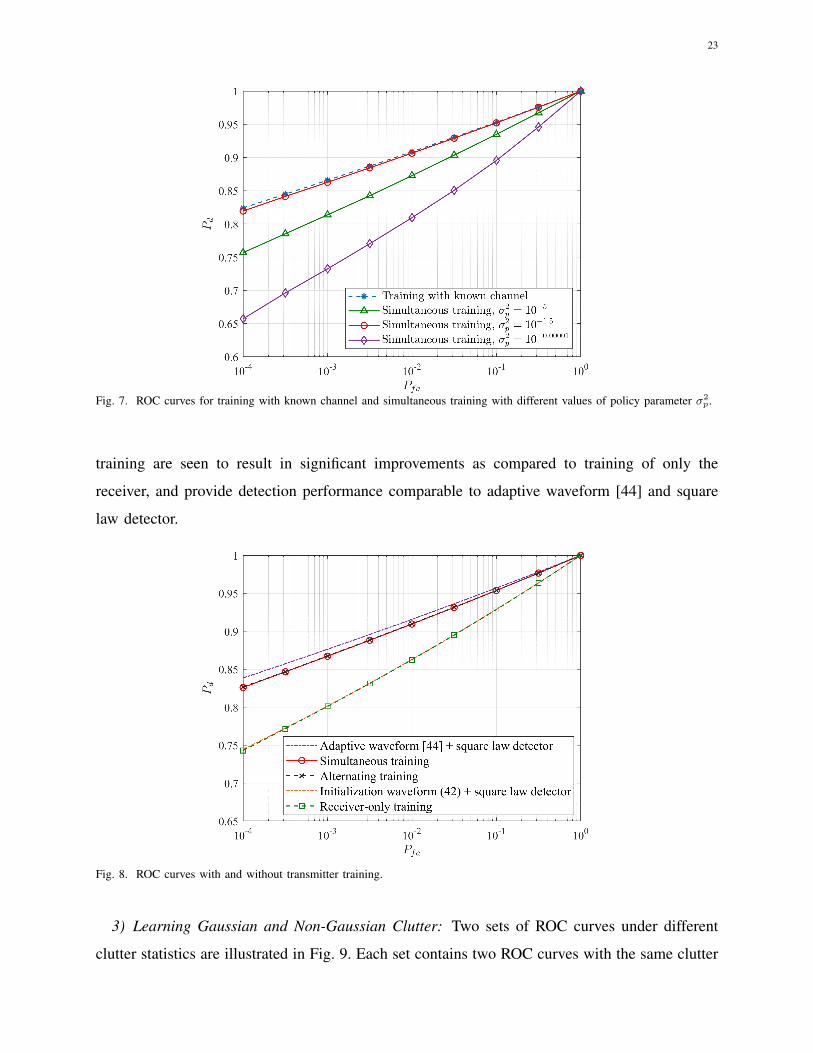
Fig. 7. ROC curves for training with known channel and simultaneous training with different values of policy parameter σ2p.

training are seen to result in significant improvements as compared to training of only the

receiver, and provide detection performance comparable to adaptive waveform [44] and square

law detector.

Fig. 8. ROC curves with and without transmitter training.

3) Learning Gaussian and Non-Gaussian Clutter: Two sets of ROC curves under different

clutter statistics are illustrated in Fig. 9. Each set contains two ROC curves with the same clutter

24

statistics: one curve is obtained based on simultaneous training, and the other one is based on

model-based design. For simultaneous training, the shape parameter of the clutter distribution

(38) in the training stage is the same as that in the test stage, i.e, βtrain = βtest. In the test stage, for

Gaussian clutter (βtest = 2), the model-based ROC curve is obtained by the adaptive waveform and

the optimal detector in the NP sense. As expected, simultaneous training provides a comparable

detection performance with the adaptive waveform and square law detector (also shown in Fig.

8). In contrast, when the clutter is non-Gaussian (βtest = 0.25), the optimal detector in the NP

sense is mathematically intractable. Under this scenario, the data-driven approach is beneficial

since it relies on data rather than a model. As observed in the figure, for non-Gaussian clutter

with a shape parameter βtest = 0.25, simultaneous training outperforms the adaptive waveform

and square law detector.

Fig. 9. ROC curves for Gaussian/non-Gaussian clutter. The end-to-end radar system is trained and tested by the same clutter

statistics, i.e, βtrain = βtest.

4) Simultaneous Training with Mixed Clutter Statistics: The robustness of the trained radar

system to the clutter statistics is investigated next. As discussed previously, model-based design

relies on a single clutter model, whereas data-driven learning depends on a training dataset. The

dataset may contain samples from multiple clutter models. Thus, the system based on data-driven

learning may be robustified by drawing samples from a mixture of clutter models. In the test stage,

the clutter model may not be the same as any of the clutter models used in the training stage.

25

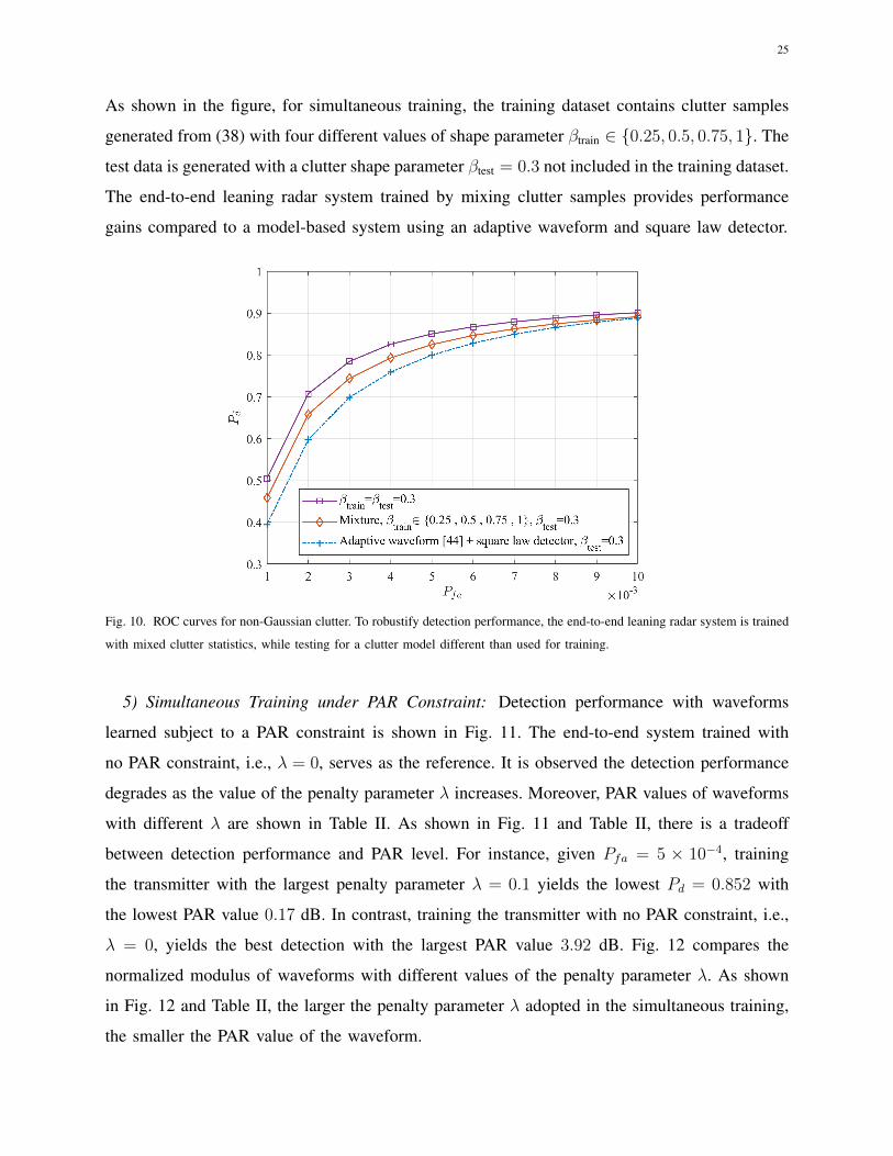
As shown in the figure, for simultaneous training, the training dataset contains clutter samples

generated from (38) with four different values of shape parameter βtrain ∈ 0.25, 0.5, 0.75, 1. The

test data is generated with a clutter shape parameter βtest = 0.3 not included in the training dataset.

The end-to-end leaning radar system trained by mixing clutter samples provides performance

gains compared to a model-based system using an adaptive waveform and square law detector.

Fig. 10. ROC curves for non-Gaussian clutter. To robustify detection performance, the end-to-end leaning radar system is trained

with mixed clutter statistics, while testing for a clutter model different than used for training.

5) Simultaneous Training under PAR Constraint: Detection performance with waveforms

learned subject to a PAR constraint is shown in Fig. 11. The end-to-end system trained with

no PAR constraint, i.e., λ = 0, serves as the reference. It is observed the detection performance

degrades as the value of the penalty parameter λ increases. Moreover, PAR values of waveforms

with different λ are shown in Table II. As shown in Fig. 11 and Table II, there is a tradeoff

between detection performance and PAR level. For instance, given Pfa = 5 × 10−4, training

the transmitter with the largest penalty parameter λ = 0.1 yields the lowest Pd = 0.852 with

the lowest PAR value 0.17 dB. In contrast, training the transmitter with no PAR constraint, i.e.,

λ = 0, yields the best detection with the largest PAR value 3.92 dB. Fig. 12 compares the

normalized modulus of waveforms with different values of the penalty parameter λ. As shown

in Fig. 12 and Table II, the larger the penalty parameter λ adopted in the simultaneous training,

the smaller the PAR value of the waveform.

26

Table II

PAR VALUES OF WAVEFORMS WITH DIFFERENT VALUES OF PENALTY PARAMETER λ

λ = 0 (reference) λ = 0.01 λ = 0.1

PAR [dB] (17) 3.92 1.76 0.17

Fig. 11. ROC curves for PAR constraint with the different values of the penalty parameter λ.

Fig. 12. Normalized modulus of transmitted waveforms with different values of penalty parameter λ.

27

6) Simultaneous Training under Spectral Compatibility Constraint: ROC curves for spectral

compatibility constraint with different values of the penalty parameter λ are illustrated in Fig.

13. The shared frequency bands are Γ1 = [0.3, 0.35] and Γ2 = [0.5, 0.6]. The end-to-end system

trained with no spectral compatibility constraint, i.e., λ = 0, serves as the reference. Training

the transmitter with a large value of the penalty parameter λ is seen to result in performance

degradation. Interfering energy from radar waveforms trained with different values of λ are

shown in Table III. It is observed that λ plays an important role in controlling the tradeoff

between detection performance and spectral compatibility of the waveform. For instance, for a

fixed Pfa = 5× 10−4, training the transmitter with λ = 0 yields Pd = 0.855 with an amount of

interfering energy −5.79 dB on the shared frequency bands, while training the transmitter with

λ = 1 creates notches in the spectrum of the transmitted waveform at the shared frequency bands.

Energy spectral densities of transmitted waveforms with different values of λ are illustrated in

Fig. 14. A larger the penalty parameter λ results in a lower amount of interfering energy in the

prescribed frequency shared regions. Note, for instance, that the nulls of the energy spectrum

density of the waveform for λ = 1 are much deeper than their counterparts for λ = 0.2.

Fig. 13. ROC curves for spectral compatibility constraint for different values of penalty parameter λ.

28

Table III

INTERFERING ENERGY FROM RADAR WAVEFORMS WITH DIFFERENT VALUES OF WEIGHT PARAMETER λ

λ = 0 (reference) λ = 0.2 λ = 1

Interfering energy [dB] (20) -5.79 -10.39 -17.11

Fig. 14. Energy spectral density of waveforms with different values of penalty parameter λ.

VI. CONCLUSIONS

In this paper, we have formulated the radar design problem as end-to-end learning of waveform

generation and detection. We have developed two training algorithms, both of which are able to

incorporate various waveform constraints into the system design. Training may be implemented

either as simultaneous supervised training of the receiver and RL-based training of the transmitter,

or as alternating between training of the receiver and of the transmitter. Both training algorithms

have similar performance. We have also robustified the detection performance by training the

system with mixed clutter statistics. Numerical results have shown that the proposed end-to-

end learning approaches are beneficial under non-Gaussian clutter, and successfully adapt the

transmitted waveform to actual statistics of environmental conditions, while satisfying operational

constraints.

29

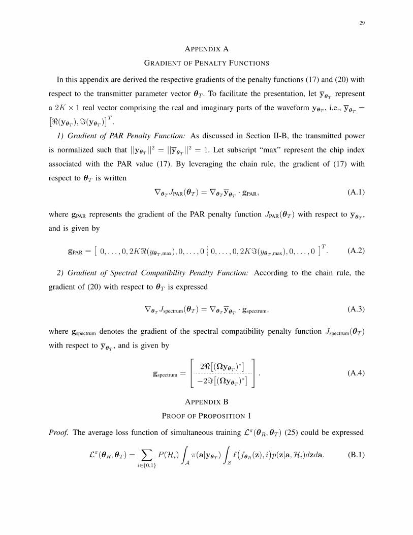
APPENDIX A

GRADIENT OF PENALTY FUNCTIONS

In this appendix are derived the respective gradients of the penalty functions (17) and (20) with

respect to the transmitter parameter vector θT . To facilitate the presentation, let yθTrepresent

a 2K × 1 real vector comprising the real and imaginary parts of the waveform yθT, i.e., yθT

=[<(yθT

),=(yθT)]T .

1) Gradient of PAR Penalty Function: As discussed in Section II-B, the transmitted power

is normalized such that ||yθT||2 = ||yθT

||2 = 1. Let subscript “max” represent the chip index

associated with the PAR value (17). By leveraging the chain rule, the gradient of (17) with

respect to θT is written

∇θTJPAR(θT ) = ∇θT

yθT· gPAR, (A.1)

where gPAR represents the gradient of the PAR penalty function JPAR(θT ) with respect to yθT,

and is given by

gPAR =[

0, . . . , 0, 2K<(yθT ,max), 0, . . . , 0 0, . . . , 0, 2K=(yθT ,max), 0, . . . , 0]T. (A.2)

2) Gradient of Spectral Compatibility Penalty Function: According to the chain rule, the

gradient of (20) with respect to θT is expressed

∇θTJspectrum(θT ) = ∇θT

yθT· gspectrum, (A.3)

where gspectrum denotes the gradient of the spectral compatibility penalty function Jspectrum(θT )

with respect to yθT, and is given by

gspectrum =

2<[(ΩyθT

)∗]

−2=[(ΩyθT

)∗] . (A.4)

APPENDIX B

PROOF OF PROPOSITION 1

Proof. The average loss function of simultaneous training Lπ(θR,θT ) (25) could be expressed

Lπ(θR,θT ) =∑i∈0,1

P (Hi)

∫Aπ(a|yθT

)

∫Z`(fθR

(z), i)p(z|a,Hi)dzda. (B.1)

30

As discussed in Section II-B, the last layer of the receiver implementation consists of a sigmoid

activation function, which leads to the output of the receiver fθR(z) ∈ (0, 1). Thus there exist a

constant b such that supz,i `(fθR

(z), i)< b <∞. Furthermore, for i ∈ 0, 1, the instantaneous

values of the cross-entropy loss `(fθR

(z), i), the policy π(a|yθT

), and the likelihood p(z|a,Hi)

are continuous in variables a and z. By leveraging Fubini’s theorem [54] to exchange the order

of integration in (B.1), we have

Lπ(θR,θT ) =∑i∈0,1

P (Hi)

∫Z`(fθR

(z), i) ∫Ap(z|a,Hi)π(a|yθT

)dadz. (B.2)

Note that for a waveform yθTand a target state indicator i, the product between the likelihood

p(z|a,Hi) and the policy π(a|yθT) becomes a joint PDF of two random variables a and z,

namely,

p(z|a,Hi)π(a|yθT) = p(a, z|yθT

,Hi). (B.3)

Substituting (B.3) into (B.2), we obtain

Lπ(θR,θT ) =∑i∈0,1

P (Hi)

∫Z`(fθR

(z), i) ∫Ap(a, z|yθT

,Hi)dadz

=∑i∈0,1

P (Hi)

∫Z`(fθR

(z), i)p(z|yθT

,Hi)dz,

(B.4)

where the second equality holds by integrating the joint PDF p(z, a|yθT,Hi) over the random

variable a, i.e.,∫A p(a, z|yθT

,Hi)da = p(z|yθT,Hi).

Taking the gradient of (B.4) with respect to θR, we have

∇θRLπ(θR,θT ) =

∑i∈0,1

P (Hi)

∫Zp(z|yθT

,Hi)∇θR`(fθR

(z), i)dz

= ∇θRLR(θR),

(B.5)

where the second equality holds via (10). Thus, the proof of Proposition 1 is completed.

31

APPENDIX C

PROOF OF PROPOSITION 2

Proof. According to (B.4), the gradient of the average loss function of simultaneous training

with respect to θT is given by

∇θTLπ(θR,θT ) =

∑i∈0,1

P (Hi)

∫Z`(fθR

(z), i)∇θT

p(z|yθT,Hi)dz

= ∇θTL(θR,θT ),

(C.1)

where the last equality holds by (33). The proof of Proposition 2 is completed.

REFERENCES

[1] S. M. Kay, Fundamentals of Statistical Signal Processing, Vol. II: Detection Theory. New York, NY, USA: Pearson, 1998.

[2] D. F. Delong, E. M. Hofstteter, “On the design of optimum radar waveforms for clutter rejection,” IEEE Trans. Inf. Theory,

vol. 13, no. 7, pp. 454-463, Jul. 1967.

[3] P. Stoica, H. He, and J. Li, “Optimization of the receive filter and transmit sequence for active sensing,” IEEE Trans. Signal

Process., vol. 60, no. 4, pp. 1730-1740, Apr. 2012.

[4] S. M. Kay, “Optimal signal design for detection of Gaussian point targets in stationary Gaussian clutter/reverberation,”

IEEE J. Sel. Topics Signal Process., vol. 1, no. 1, pp. 31-41, Jun. 2007.

[5] M. A. Richards, J. A. Scheer, and W. A. Holm, Principles of Modern Radar. Edison, NJ, USA: Scitech Pub., 2010.

[6] F. Gini, A. De Maio, and L. Patton, Waveform Design and Diversity for Advanced Radar Systems. London, UK: Inst. Eng.

Technol., 2012.

[7] H. L. Van Trees, Detection, Estimation, and Modulation Theory, Part I: Detection, Estimation and Linear Modulation Theory.

New York, NY, USA: John Wiley & Sons, 2004.

[8] D. P. Meyer and H. A. Mayer, Radar Target Detection. New York, NY, USA: Academic Press, 1973.

[9] M. A. Richards, Fundamentals of Radar Signal processing. New York, NY, USA: McGraw-Hill, 2005.

[10] K. J. Sangston and K. R. Gerlach, “Coherent detection of radar targets in a non-Gaussian background,” IEEE Trans. Aerosp.

Electron. Syst., vol. 30, no. 2, pp. 330-340, Apr. 1994.

[11] F. Gini, “Sub-optimum coherent radar detection in a mixture of K-distributed and Gaussian clutter,” in Proc. IEE Radar,

Sonar and Navigat., vol. 144, no. 1, pp. 39-48, Feb. 1997.

[12] K. J. Sangston, F. Gini, M. V. Greco, and A. Farina, “Structures for radar detection in compound Gaussian clutter,” IEEE

Trans. Aerosp. Electron. Syst., vol. 35, no. 2, pp. 445-458, Apr. 1999.

[13] A. Farina, A. Russo, and F. A. Studer, “Coherent radar detection in log-normal clutter,” IEE Proc. F, Commun. Radar and

Signal Process., vol. 133, no. 1, Feb. 1986.

[14] F. A. Pentini, A. Farina, and F. Zirilli, “Radar detection of targets located in a coherent K-distributed clutter background,”

IEE Proc. F, Radar and Signal Process., vol. 139, no. 3, pp. 239-245, Jun. 1992.

[15] S. M. Kay, “Waveform design for multistatic radar detection,” IEEE Trans. Aerosp. Electron. Syst., vol. 45, no. 4, pp.

1153-1165, Jul. 2009.

32

[16] M. M. Naghsh, M. Modarres-Hashemi, S. Shahbazpanahi, M. Soltanalian, and P. Stoica, “Unified optimization framework

for multi-static radar code design using information-theoretic criteria,” IEEE Trans. Signal Process., vol. 61, no. 21, pp.

5401-5416, Nov. 2013.

[17] S. Khalili, O. Simeone and A. Haimovich, “Cloud radio-multistatic radar: Joint optimization of code vector and backhaul

quantization,” IEEE Signal Process. Lett., vol. 22, no. 4, pp. 194-498, Apr. 2015.

[18] S. Jeong, S. Khalili, O. Simeone, A. Haimovich, and J. Kang, “Multistatic cloud radar systems: Joint sensing and

communication design,” Trans. Emerg. Telecommun. Technol., vol. 27, no. 5, pp. 716-730, Feb. 2016.

[19] A. De Maio, Y. Huang, M. Piezzo, S. Zhang, and A. Farina, “Design of optimized radar codes with a peak to average

power ratio constraint,” IEEE Trans. Signal Process., vol. 59, no. 6, pp. 2683-2697, Jun. 2011.

[20] B. Tang, M. M. Naghshm, and J. Tang, “Relative entropy-based waveform design for MIMO radar detection in the presence

of clutter and interference,” IEEE Trans. Signal Process., vol. 63, no. 14, pp. 3783-3796, Apr. 2015.

[21] M. M. Naghsh, M. Modarres-Hashemi, M. A. Kerahroodi, and E. H. M. Alian, “An information theoretic approach to

robust constrained code design for MIMO radars,” IEEE Trans. Signal Process., vol. 65, no. 14, pp. 3647-3661, Jul. 2017.

[22] L. Wu, P. Badu, and D. P. Palomar, “Transmit waveform/receive filter design for MIMO radar with multiple waveform

constraints,” IEEE Trans. Signal Process., vol. 66, no. 6, pp. 1526-1540, Mar. 2018.

[23] G. Locke and L. E. Strickling, “An assessment of the near-term viability of accommodating wireless broadband systems

in the 1675-1710 MHz, 1755-1780 MHz, 3500-3650 MHz, 4200-4220 MHz, and 4380-4400 MHz bands (Fast Track

Evaluation Report),” Oct. 2010. [Online]. Available: https://www.ntia.doc.gov/files/ntia/publications/fasttrackevaluation

11152010.pdf

[24] A. Aubry, V. Carotenuto, A. De Maio, A. Farina and L. Pallotta, “Optimization theory-based radar waveform design for

spectrally dense environments,” IEEE Aerosp. Electron. Syst. Mag., vol. 31, no. 12, pp. 14-25, Dec. 2016.

[25] W. Jiang and A. M. Haimovich, “Joint optimization of waveform and quantization in spectral congestion conditions,” in

Proc. 52nd Asilomar Conf. Signals, Syst., Comput., Oct. 2018, pp. 1897-1898.

[26] L. Zheng, M. Lops, X. Wang, and E. Grossi, “Joint design of overlaid communication systems and pulse radars,” IEEE

Trans. Signal Process., vol. 66, no. 1, pp. 139-154, Jan. 2018.

[27] W. Jiang and A. M. Haimovich, “Waveform optimization in cloud radar with spectral congestion constraints,” in Proc.

IEEE Radar Conf., Apr. 2019, pp. 1-6.

[28] B. Tang and J. Li, “Spectrally constrained MIMO radar waveform design based on mutual information,” IEEE Trans. Signal

Process., vol. 67, no. 3, pp. 821-834, Feb. 2019.

[29] N. Sebe, I. Cohen, A. Garg, and T. S. Huang, Machine Learning in Computer Vision. Heidelberg, Germany: Springer, 2005.

[30] J. Deng, W. Dong, R. Socher, L. Li, K. Li and L. Fei-Fei, “ImageNet: A large-scale hierarchical image database,” in Proc.

IEEE Conf. on Computer Vision and Pattern Recognition, Jun. 2009, pp. 248-255.

[31] T. Young, D. Hazarika, S. Poria, and E. Cambria, “Recent trends in deep learning based natural language processing,”

IEEE Comput. Intell. Mag., vol. 13, no. 3, pp. 55-75, Aug. 2018.

[32] J. Devlin, M. W. Chang, K. Lee, and K. Toutanova, “Bert: Pre-training of deep bidirectional transformers for language

understanding,” arXiv preprint arXiv:1810.04805, 2018.

[33] T. O’Shea and J. Hoydis, “An Introduction to deep learning for the physical layer,” IEEE Trans. Cogn. Commun. Netw.,

vol. 3, no. 4, pp. 563-575, Dec. 2017.

[34] O. Simeone, “A brief introduction to machine learning for engineers,” Found. Trends® Signal Process., vol. 12, no. 3-4,

pp. 200-431, Aug. 2018.

[35] M. Kim, W. Lee, and D. H. Cho, “A novel PAPR reduction scheme for OFDM system based on deep learning,” IEEE

Commun. Lett., vol. 22, no. 3, pp. 510-513, Mar. 2018.

33

[36] F. A. Aoudia and J. Hoydis, “Model-free training of end-to-end communication systems,” IEEE J. Sel. Areas Commun.,

vol. 37, no. 11, pp. 2503-2516, Nov. 2019.

[37] V. Raj and S. Kalyani, “Backpropagating through the air: Deep learning at physical layer without channel models,” IEEE

Commun. Lett., vol. 22, no. 11, pp. 2278-2281, Nov. 2018.

[38] O. Simeone, “A very brief introduction to machine learning with applications to communication systems,” IEEE Trans.

Cogn. Commun. Netw., vol. 4, no. 4, pp. 648-664, Dec. 2018.

[39] O. Simeone, S. Park, and J. Kang, “From learning to meta-learning: Reduced training overhead and complexity for

communication systems,” in Proc. 6G Wireless Summit, Mar. 2020.

[40] S. Park, O. Simeone, and J. Kang, “Meta-learning to communication: Fast end-to-end training for fading channels,” in

Proc. IEEE 45th Int. Conf. Acoustic, Speech and Signal Process. (ICASSP), May 2020.

[41] S. Park, O. Simeone, and J. Kang, “End-to-end fast training of communication links without a channel model via online

meta-learning,” arXiv preprint arXiv:2003.01479, 2020.

[42] M. P. Jarabo-Amores, M. Rosa-Zurera, R. Gil-Pita, and F. Lopez-Ferreras, “Study of two error functions to approximate the

Neyman-Pearson detector using supervised learning machines,” IEEE Trans. Signal Process., vol. 57, no. 11, pp. 4175-4181,

Nov. 2009.

[43] M. P. Jarabo-Amores, D. de la Mata-Moya, R. Gil-Pita, and M. Rosa-Zurera, “Radar detection with the Neyman–Pearson

criterion using supervised-learning-machines trained with the cross-entropy error,” EURASIP Journal on Advances in Signal

Process., vol. 2013, no. 1, pp. 44-54, Mar. 2013.

[44] W. Jiang, A. M. Haimovich, and O. Simeone, “End-to-end learning of waveform generation and detection for radar

systems,” in Proc. IEEE 53rd Asilomar Conf. on Signals, Systems, and Computers, Nov. 2019, pp. 1672-1676.

[45] I. Goodfellow, Y. Bengio, and A. Courville, Deep Learning. Cambridge, MA, USA: MIT Press, 2016.

[46] S. Ruder, “An overview of gradient descent optimization algorithms,” arXiv preprint arXiv:1609.04747, 2016.

[47] R. S. Sutton, D. A. McAllester, S. P. Singh, and Y. Mansour, “Policy gradient methods for reinforcement learning with

function approximation,” Adv. Neural Inf. Process. Syst., vol. 12, 2000.

[48] A. Aubry, A. De Maio, Y. Huang, M. Piezzo, and A. Farina, “A new radar waveform design algorithm with improved

feasibility for spectral coexistence,” IEEE Trans. Aerosp. Electron. Syst., vol. 51, no. 2, pp. 1029-1038, Apr. 2015.

[49] D. Silver, G. Lever, N. Heess, T. Degris, D. Wierstra, and M. Riedmiller, “Deterministic policy gradient algorithms,” in

Proc. Int. Conf. Machine Learning, 2014, pp. 387–395.

[50] A. Farina, A. Russo, F. Scannapieco, and S. Barbarossa, “Theory of radar detection in coherent Weibull clutter,” IEE Proc.

F, Commun., Radar and Signal Process., vol. 134, no. 2, pp. 174-190, Apr. 1987.

[51] D. A. Shnidman, “Generalized radar clutter model,” IEEE Trans. Aerosp. Electron. Syst., vol. 35, no. 3, pp. 857-865, Jul.

1999.

[52] D. Clevert, T. Unterthiner, and S. Hochreiter, “Fast and accurate deep network learning by exponential linear units (ELUs),”

in Proc. Int. Conf. Learn. Represent., May 2016, pp. 1-14.

[53] D. Kingma and J. Ba, “Adam: A method for stochastic optimization,” in Proc. Int. Conf. Learn. Represent., May 2015, pp.

1-15.

[54] W. Rudin, Real and Complex Analysis. New York, NY, USA: McGraw-Hill, 1987.