Embed Size (px)
Citation preview
Research ArticleJoint Decision on Ordering and Pricing of Cruise TourismSupply Chain with Competing Newsboy-Type Retailers
Miaoqing Shi and Bin Liu
School of Economics and Management Shanghai Maritime University Shanghai 201306 China
Correspondence should be addressed to Bin Liu liubinshmtueducn
Received 21 May 2018 Revised 15 June 2018 Accepted 28 June 2018 Published 26 July 2018
Academic Editor Honglei Xu
Copyright copy 2018 Miaoqing Shi and Bin Liu This is an open access article distributed under the Creative Commons AttributionLicense which permits unrestricted use distribution and reproduction in any medium provided the original work is properlycited
Cruise industry has recorded rapid expansion during the last decades and it has substantial contribution to local economies In thispaper we introduce a cruise tourism supply chain system consisting of one supplier and two newsboy-type retailers We investigatethe optimal decisions in a decentralized system from a game theoretical perspective and find out the optimal ordering and pricingstrategies of both retailers and the optimal wholesale prices of the supplier with the limited number of cruise tickets and try tofind out how the total profits should be allocated by the two retailers in the alliance case Our framework involves two operationalstrategies including inconsistent wholesale prices in the benchmark case and consistent wholesale price in the alliance case inwhichthe two retailers have a virtual alliance combining to one retailer A numerical example compares the performance of the supplychain members and the system in two cases and finds that it is better for the two retailers to have a virtual alliance combining toone retailer when the total amount of cruise tickets ordered by the two retailers is constrained by the total number of cruise ticketsfor the supplier but it is not good choice for the two retailers to combine to one retailer when the total number of cruise ticketsfor the supplier does not constrain the total amount of cruise tickets ordered by the two retailers In addition the performance ofthe system in the alliance case is as good as that in the benchmark case when the total amount of cruise tickets ordered by the tworetailers is constrained by the total number of cruise tickets for the supplier However when the total number of cruise tickets forthe supplier does not constrain the total amount of cruise tickets ordered by the two retailers the performance of the system in thebenchmark case is better than that in the alliance case
1 Introduction
In recent years we have witnessed a period of rapid growthand remarkable change in the cruise industry which is one ofthe fastest growing and most dynamic segments of the entiretourism and leisure travel market [1 2] According to CruiseMarketWatch the number of passengers is projected to growto 25 million in 2019 with an average growth rate of 45[3] The substantial spending of cruise passengers togetherwith the high growth rates indicates that the cruise industryhas great market potential Therefore policy makers andresearchers have paid close attention to the economic impactsof cruise tourism at the national or regional level [4] Changand Lee et al [3] build a network DEA model to elaboratethe operation of cruise lines at two stages for the purposeof analyzing the financial statements of the lines However
we investigate the supply chain management problem of thecruise industry in China
In terms of the cruise industry it may be differentfrom the other industries in several ways First there is nosalvage of the cruise tickets in one trip but many productssuch as garment and mobile phone often have salvage aftera period Second there is a nature partnership betweenthe downstream retailers That is when one retailerrsquos orderquantity of cruise tickets is less than the customers demandthen they can reorder the cruise tickets from the otherretailer by a higher reorder cost which is similar to theemergency procurement behavior in Zhang and Liu [5] Butit is uncommon in other industries because there alwaysonly exist competition between retailers in general case thatis there is no specific cooperation between retailers Thirdbecause of the characteristics of cruise industry operation
HindawiMathematical Problems in EngineeringVolume 2018 Article ID 3516785 16 pageshttpsdoiorg10115520183516785
2 Mathematical Problems in Engineering
there is almost no centralized system in the cruise industrySuppliers and retailers compete with each other while otherindustries may have centralized systems Finally the totalnumber of cruise tickets for the supplier is fixed over arelatively long time because the size of the cruise is fixed andthe number of cruise beds is limited and itmay hold a limitednumber of customers during one trip It is impossible for thesupplier to satisfy the total amount of cruise tickets ordered bydownstream retailers when the total number of cruise ticketsfor the supplier is smaller than the total amount of cruisetickets ordered by retailers But for the other industriesit may always occur that the supplier can satisfy the totalamount ordered by the retailers and one can take no accountof the limited number of products for the supplier
Supply chain management has been studied by manyresearchers however it always refers to ordinary productsseasonal products or other related products These prod-ucts often involve the passing of property but the sale ofcruise tickets may more involve the right of use to thecruise in one trip That may be a difference between thecruise tourism supply chain management problem and otherindustries supply chain management issues In addition asfor the two-echelon cruise tourism supply chain there willalways be competition between the upstream supplier andthe downstream retailers like other industries supply chainand in reality the competing retailers in the cruise industrycan use alliance to counter the monopoly of supplier andthe paper considers the strategic alliance between the tworetailers whether being better off to both retailers or not andcorrespondingly we analyze the performance difference ofthe supplier and the system between the benchmark (withoutalliance) case and the alliance case
In this paper we address the cruise tourism supply chainconsisting of one supplier-cruise owner and two competingretailers with the limited number of cruise tickets for thesupplier under stochastic demand and we find that themaximum profit function of the supplier is continuous andconcave so the optimal solution to the wholesale ticketprice of the supplier exists and it is the one and onlysolution the maximum expected profit functions of bothretailers are also continuous and concave and the optimalsolutions to the retail ticket price and order quantity of cruisetickets for both retailers exist and that is the one and onlysolution and then this paper illustrates that the optimalwholesale ticket price of the supplier is not affected by themarket potentials of both retailers in the alliance case thatis the optimal wholesale ticket price in the alliance case isdecided by supplier without considering themarket potentialof both retailers or the market potential gap between thetwo retailers We are particularly interested to see what theperformance difference of the supply chain members andthe system is between in the benchmark scenario and inthe alliance scenario with a certain number of cruise ticketsfor the supplier and we study the optimal decisions of thesupplier and both retailers in the two scenarios Furthermorethe paper numerically investigates the impacts of relatedparameters on the supplierrsquos profit the two retailersrsquo expectedprofits the systemrsquos expected profit the optimal pricing andordering decisions of both retailers and the optimal pricing
decision of the supplier In addition our work considers theprofits allocation between the two retailers in the alliancecase and the paper gives some useful management insightsinto the economic behaviors of cruise firms We assume thatall parameters and states are considered common knowledgeso that all players have full information [6] and when eachof the two retailers has no enough number of cruise tickets tocustomers the retailer can reorder the insufficient number ofcruise tickets using more than the wholesale price costs fromthe other retailer The two retailers are in the same marketand compete with each other in the benchmark case and thetwo retailers cooperate to have a virtual alliance combiningto one retailer to weaken the supplierrsquos monopoly position inthe alliance case
The relevant literature can be divided into three researchstreams joint decision onpricing and ordering researchmul-tiechelon supply chain research and competitive researchThe newsvendor model is necessitated by the pricing andordering decisions under uncertain demand And our workis closely related to the newsvendor setting literature Whitin[7] is the first to formulate a newsvendor model with priceeffects In his model selling price and stocking quantityare set simultaneously Petruzzi and Dada [8] review thenewsvendor problemand formulate a randomness in demandwhich is price independent model either in an additive or ina multiplicative fashion Hua andWang et al [9] consider thenewsvendor problem that incorporates price decision withfree shipping using the two fashions
In the operations management research joint decisionpricing and ordering research is not uncommon Fu and Danet al [10] present a joint decisions model in a newsvendorsetting where a retailer sells the seasonal products at theweather-dependent prices and provide a detailed analysis ofthe problems and characterizations of the optimal decisionswhen the retailer is risk-neutral Wu and Zhang [11] studyordering and pricing problems for new repeat-purchaseproducts and incorporate the repeat-purchase rate and priceeffects into the Bass model to characterize the demand pat-ternwhich considers two decisionmodels two-stage decisionmodel and joint decision model Liu and Zhang et al [12]investigate online dual channel supply chain system and itsjoint decision on production and pricing under informationasymmetry They extend a newsvendor framework to dualchannel in which there exists competitions and apply thecompetitive stochastic customer demand functions to thedual channel supply chain management
Because the overall system sometimes should be consid-ered in the supply management multiechelon supply chainis widely studied Tiaojun and Gang et al [13] study thecoordination of the supply chain in which there are onemanufacturer and two competing retailers with demand dis-ruptions and consider a price-subsidy rate contract to coor-dinate the investments of the competing retailers with salespromotion opportunities and demand disruptions Cachonand Zipkin [14] investigate a two-stage serial supply chainwith stationary stochastic demand and fixed transportationtimes Qi and Wang et al [15] consider a two-echelon make-to-order supply chain consisting of one supplier and tworetailers under carbon cap regulation and analyze the pricing
Mathematical Problems in Engineering 3
decision process in a decentralized system from a gametheoretical perspective
Competitive research is challenging but competition isalso more in line with the actual situation so many scholarsstudy the optimization of supply chain from the perspectiveof competition Parthasarathi and Sarmah et al [16] study thesupply chain coordination under retail competition using anewsvendor framework in which the random demand facedby each retailer is dependent on their own price as wellas on the price of the competing retailer In addition tothis the demand is also influenced by the initial stock levelof each individual retailer Bernstein and Federgruen [17]and Narayanan and Raman et al [18] investigate decentral-ized supply chains with competing retailers under demanduncertainty and design contractual arrangements betweenthe parties that allow the decentralized chain to performas well as a centralized one In addition Liu and Zhang etal [12] extend a newsvendor framework to dual channel inwhich there exists competitions and apply the competitivestochastic customer demand functions to the dual channelsupply chain management and Qi and Wang et al [15]study a make-to-order supply chain with one supplier andtwo competing retailers under a carbon cap regulation andformulate different pricingmodels and analyze the respectivepricing processes under a carbon cap regulation in a decen-tralized system considering the competition between the tworetailers
Our work is closely related to Qi and Wang et al [15]but differs from Qi and Wang et al [15] in several mannersFirst the demand is deterministic of the two-echelon supplychain in their work but our work studies the randomdemand Second they consider an external constraint-carboncap regulation-imposed on the supply chain however ourwork considers the internal constraint of the limited numberof cruise tickets for the supplier Third their frameworkinvolves various operational strategies including consistentand inconsistent wholesale prices for the supplier and consis-tent and inconsistent retail prices for the two retailers but ourframework involves only two different pricing strategies andwe consider how the total expected profits of both retailersin the alliance case should be allocated by the two retailersin which case both retailers launch an alliance against themonopoly position of the supplier in cruise industry Ourmodel is most closely related to Liu and Zhang et al [12]Liu and Zhang et al [12] set a dual channel newsvendormodel and investigate online dual channel supply chainsystem and its joint decision on production and pricingunder information asymmetry they take more considerationto the impact of information on retailerrsquos optimal decisionsand profits of the supplier and retailer But our work has toconsider the limited number of cruise tickets for the supplier
This paper considers the limited number of cruise ticketsfor the supplier and the two retailers may follow a policywhich is similar to the ldquobase-stockrdquo policy Federgruen andZipkin [19] demonstrate that a modified base-stock policy isoptimal for a single-stage capacitated inventory system overan infinite horizon this policy recommends ordering up toa particular inventory level if possible but to the capacitylevel otherwise And in the optimal decisions process similar
to Ben Daya and Raouf [20] that develop a Lagrange basedmethod for solving two-constraint problem with uniformdemand distribution we also solve the limited number ofcruise tickets constraint problem using a Lagrange basedmethod and we develop a solution method based on Kuhn-Tucker (K-T) conditionswhich produces the optimal solutionto the problem with any continuous demand distributionsimilar to Zhang [21] In addition when the two retailerslaunch a virtual alliance combining to one retailer in thealliance case we establish a bargaining game similar to Selcukand Gokpinar [22] in order to satisfy each of the bothretailers
The paper is structured as follows In Section 2 wedescribe the model and provide some notations and assump-tions Section 3 solves the optimal decisions of the supplierand two retailers in the benchmark case Section 4 dealswith the optimal decisions of the supplier and two retailersin the alliance case as well as the total profitsrsquo allocationbetween the two retailers Section 5 based on a numericalexample illustrates different optimal decisions under twocases and sensitivity to critical parameters and it allows usto interpret the effects of market potential of the two retailersand competition between them on profits We conclude inSection 6 Proofs appear in the Appendix
2 Modeling and Assumptions
Thepaper considers a two-echelon supply chain consisting ofone supplier and two retailers under stochastic demand withthe limited number of cruise tickets for the supplier Becausein the cruise industry there are few cases of centralizedsystem then we discuss two cases (the benchmark case1198821 =1198822 and the alliance case1198821 = 1198822 = 1198820) in the decentralizedsystem
21 The Notations and Assumptions For the stochastic cus-tomer demand we denote the demand function of bothretailers as follows
1198631 (1198751 1198752) = 1199101 (1198751 1198752) + 11990911199101 (1198751 1198752) = 120579 minus 1198751 + 1205731198752 (1)
and 1198632 (1198751 1198752) = 1199102 (1198751 1198752) + 11990921199102 (1198751 1198752) = 1 minus 120579 minus 1198752 + 1205731198751 (2)
120579 which is a parameter represents the market potentialof retailer 1199031 120573 is called the cross-price-sensitivity coefficientwhich implies the intensity of competition between the tworetailers and 119909119894 is the random variable of retailerrsquos 119903119894 (119894 = 1 2)demand with the mean 120583119894 (119894 = 1 2) in our model and let1205831 = 1205832 = 0 and the density function 119891119894(∙) have a continuousderivative 1198911015840119894 (∙) [16] and 1198911015840119894 (∙) ge 0 in our model The majornotations used in this paper are listed in Table 1
Consistent with Petruzzi and Dada [8] we define
1199111 = 1198761 minus 1199101 (1198751 1198752) 1199112 = 1198762 minus 1199102 (1198751 1198752) (3)
4 Mathematical Problems in Engineering
Table 1 Major notations
119888 The unit operating cost of the supplier1198790 The total number of cruise tickets for the supplier120579 Market potential composed of the retailer 1199031120573 Cross price elastic coefficient
119892 The cost per unit when the amount of cruise tickets ordered by a retailer less than the demand of consumersthen to reorder from the other retailer
119882119894 The unit wholesale ticket price of the supplier to retailer 119903119894 (119894 = 1 2) in the benchmark case1198820 The unit wholesale ticket price of the supplier to retailer 119903119894 (119894 = 1 2) in the alliance case119875119894 The unit retail ticket price of the retailer 119903119894 (119894 = 1 2) in the benchmark case1198751015840119894 The unit retail ticket price of the retailer 119903119894 (119894 = 1 2) in the alliance case119876119894 The retailer 1199031198941015840119904 (119894 = 1 2) order quantity of cruise tickets in the benchmark case1198761015840119894 The retailer 1199031198941015840119904 (119894 = 1 2) order quantity of cruise tickets in the alliance case120582 Lagrange multiplier in the benchmark case1205821015840 Lagrange multiplier in the alliance case119909119894 The random variable of retailerrsquos 119903119894 (119894 = 1 2) demand119891119894 (∙) The PDF(Probability Density Function) of random variable 119909119894 (119894 = 1 2)119865119894 (∙) The CDF(Cumulative Distribution Function) of random variable 119909119894 (119894 = 1 2)119865minus1119894 (∙) The inverse Cumulative Distribution Function of random variable 119909119894 (119894 = 1 2)Note the subscripts ldquorrdquo and ldquosrdquo are added to the relative variables to represent the values of the retailer and supplier respectively the subscripts ldquo1rdquo and ldquo2rdquo areadded to the relative variables to represent the values of the retailer r1 and r2 respectively the subscript ldquoTrdquo is added to the relative variables to represent thevalues of the system and the superscripts ldquolowastrdquo and ldquo 1015840rdquo are added to the relative variables to represent their corresponding optimal values and the correspondingvalues in the alliance case respectively and the expected profits in the benchmark case and the alliance case are denoted asΠ(sdot) Π1015840(sdot) respectively
11991110158401 = 11987610158401 minus 11991010158401 (11987510158401 11987510158402) 11991110158402 = 11987610158402 minus 11991010158402 (11987510158401 11987510158402)
(4)
where 119876119894 (119894 = 1 2) is the retailerrsquos order quantity ofcruise tickets in the benchmark case and 1198761015840119894 (119894 = 1 2) is theretailerrsquos order quantity of cruise tickets in the alliance case
And there are also some assumptions made in our model(1)The total market potential equals 1 and 120579 (120579 isin [0 1])represents the market potential of retailer 1199031 1 minus 120579 representsthe market potential of retailer 1199032 and then we also assumethat 120579 ge 12 implying that themarket potential of the retailer1199031 is bigger than or equal to themarket potential of the retailer1199032 (2)Theprice-sensitivity coefficient of every retailer equals120573 and 120573 lt 1 (120573 isin [0 1]) implying that the demand of retailer119903119894 (119894 = 1 2) is more sensitive to 119875119894 than the rivalrsquos price(3) 119892 gt 119882119894 gt 119888(119894 = 0 1 2) implying that the reordercost when one retailerrsquos order quantity of cruise tickets isless than the customers demand and then to order from theother retailer is larger than the wholesale ticket price from thesupplier and thewholesale ticket price of the supplier is largerthan the operating cost of his own(4) The total number of cruise tickets levels at thebeginning of the period Both retailers know the total numberof cruise tickets levels for the supplier at the beginningof the period which was similarly assumed by Parker andKapuscinski [6](5) All the demands of customers must be met at alltimes and the retailersmust ensure satisfying the demands of
customers through a cost which is larger than the wholesaleticket price and swift transportation from the other retailer toprovide to customers [5 12](6) All members in the cruise industry supply chain arerisk-neutral The market information is a common knowl-edge and retailers are assumed to be operating in the samemarketplace and all of them seek the maximization of theirown expected profit
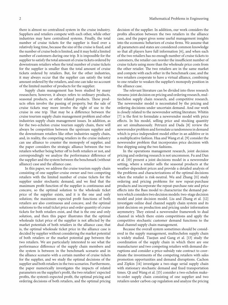
22 Modeling Formulation In this paper the supplier hasa certain number of cruise tickets with a constant unitoperating cost c and the supplier determines the wholesaleticket prices to the two retailers Both retailers operate inthe same marketplace and compete with each other [6]and the two retailers respectively determine the retail ticketprices 1198751 1198752 and the order quantities of cruise tickets 11987611198762 simultaneously with the fixed number of cruise tickets1198790 for the supplier We study a decentralized system in twocases which are the benchmark case (1198821 = 1198822) and thealliance case (1198821 = 1198822 = 1198820) and we want to comparethe performance of the supply chainmembers and the systembetween them in the benchmark case and in the alliance casewhere the two retailers have a virtual alliance combiningto one retailer And the two-echelon cruise tourism supplychain is illustrated by Figure 1 where the benchmark case isrepresented in Figure 1(a) and the alliance case is representedin Figure 1(b)
We model the decisions process of the system as a Stack-elberg game in which the supplier is the leader and the tworetailers are the follower In this system the decisions process
Mathematical Problems in Engineering 5
market demand
supplier
retailer2retailer1
c T0
W1
W2
Q1 Q2
P1 P2
(a)
c
supplier
retailer1 retailer2
market demand
retailer
T0
W0
W0W0
Q1
Q1
+Q2
Q2
P1
P2
(b)
Figure 1 The two-echelon cruise tourism supply chain with one supplier and two retailers in two cases
is that the supplier first determines the wholesale ticket prices1198821 and 1198822 in the benchmark case or 1198820 in the alliancecase and then the two retailers respectively determine theirown retail ticket price and the order quantity of cruisetickets simultaneously In addition the cruise industry has nosalvage value then the model in the paper is equal to a modelwhich is salvaged at 0 similar to Luo and Sethi et al [23]
Under this system the expected profit functions of bothretailers in the benchmark case are
Π119903119894 (119875119894 119876119894) = 119864 (120587 (119903119894)) = 119864 (119875119894 lowast 119863119894 (1198751 1198752) minus 119882119894lowast 119876119894 minus 119892 lowast [119863119894 (1198751 1198752) minus 119876119894]+) (119894 = 1 2) (5)
where [∙]+ = max∙ 0Given the retail ticket price and the order quantity of
cruise tickets the retailerrsquos revenue is shown in the first termthe second term is the purchasing cost from the supplier andthe last term is the purchasing cost from the other retailerwhen the demand of consumers is larger than hisher orders
The profit of the supplier in the benchmark case isΠ119904 (11988211198822) = 11988211198761 +11988221198762 minus 1198881198790 (6)
Accordingly the expected profit functions of both retailers inthe alliance case can be formulated by
Π1015840119903119894 (11987510158401198941198761015840119894) = 119864 (1205871015840 (119903119894)) = 119864 (1198751015840119894 lowast 119863119894 (11987510158401 11987510158402)minus1198820 lowast 1198761015840119894 minus 119892 lowast [119863119894 (11987510158401 11987510158402) minus 1198761015840119894]+)
(119894 = 1 2) (7)
Themeaning of each term in this expression is similar to thatin (5)
The profit of the supplier in the benchmark case can beformulated by
Π1015840119904 (1198820) = 1198820 (11987610158401 + 11987610158402) minus 1198881198790 (8)
The supplier and two retailers in two cases all operate tomaximize their own expected profit
3 Optimal Joint Decisions inthe Benchmark Case
In this section the supplier sets the wholesale price dis-crimination to the two retailers because of the differentmarket potential of both retailers and we use the backwardsequential decision-making approach to obtain the optimalsolutions
31 Joint Decision on Pricing and Ordering of the Two Retailersin the Benchmark Case From (1)-(5) and 1205831 = 1205832 = 0 wecan obtain the expected profit functions of both retailers inthe benchmark case as followsΠ119903119894 (119875119894 119911119894) = 119875119894 lowast 119910119894 (1198751 1198752) minus 119882119894 lowast (119910119894 (1198751 1198752) + 119911119894)+ 119892 lowast (119911119894 minus Θ119894 (119911119894)) (119894 = 1 2) (9)
where Θ119894(119911119894) = int119911119894minus119886119894(119911119894 minus 119909119894) lowast 119891119894(119909119894)119889119909119894(119894 = 1 2)We can formulate the Stackelberg game model under this
system in the benchmark case as follows
6 Mathematical Problems in Engineering
max(11988211198822)
Π119904 = 1198821 lowast (1199101 (119875lowast1 119875lowast2 ) + 119911lowast1 ) + 1198822 lowast (1199102 (119875lowast1 119875lowast2 ) + 119911lowast2 ) minus 1198881198790st 1199101 (119875lowast1 119875lowast2 ) + 119911lowast1 + 1199102 (119875lowast1 119875lowast2 ) + 119911lowast2 le 1198790
119875lowast1 119875lowast2 119911lowast1 119911lowast2 is derived from solving the following problem
max(1198751 1199111)
Π1199031 = 1198751 lowast 1199101 (1198751 1198752) minus 1198821 lowast (1199101 (1198751 1198752) + 1199111) + 119892 lowast (1199111 minus Θ1 (1199111))max(1198752 1199112)
Π1199032 = 1198752 lowast 1199102 (1198751 1198752) minus 1198822 lowast (1199102 (1198751 1198752) + 1199112) + 119892 lowast (1199112 minus Θ2 (1199112))
(10)
Using the backward sequential decision-makingapproach in this model both retailersrsquo response functions forthe given wholesale prices1198821 and1198822 in the benchmark casemay be obtained as follows
119875lowast1 = 21198821 + 1205731198822 + 120573 + (2 minus 120573) 1205794 minus 1205732119875lowast2 = 21198822 + 1205731198821 + 120573 + (2 minus 120573) (1 minus 120579)4 minus 1205732119876lowast1 = (1205732 minus 2)1198821 + 1205731198822 + 120573 + (2 minus 120573) 1205794 minus 1205732
+ 119865minus11 (119892 minus1198821119892 )
119876lowast2 = (1205732 minus 2)1198822 + 1205731198821 + 120573 + (2 minus 120573) (1 minus 120579)4 minus 1205732+ 119865minus12 (119892 minus1198822119892 )
(11)
Fromboth retailersrsquo response functions we can obtain thefollowing proposition
Proposition 1 The retail ticket prices of both retailers areincreasing with the increasing intensity of competition betweenthe two retailers for the given values of W1 and W2
Form Proposition 1 we know that the greater the com-petition between the two retailers the larger the retail ticketprices of both retailers that is the retail ticket prices ofboth retailers are increasing with increasing the degree of thesubstitution between the two retailers
32 Decision on Wholesale Ticket Prices of the Supplier in theBenchmark Case Under this system the supplier determinesthe optimal wholesale ticket prices 119882lowast1 and 119882lowast2 to the tworetailers differently in the benchmark case based on theexisting number of cruise tickets for the supplier From thegamemodel in the benchmark case we can have the followingproposition
Proposition 2 The optimal wholesale ticket prices of thesupplier in the benchmark case can be given by
(i)
[1 minus 1198911 lowast (1198601 minus 119892)]1198821 minus 1198911 lowast 119865minus11 (119892 minus1198821119892 ) = 0
[1 minus 1198912 lowast (1198602 minus 119892)]1198822 minus 1198912 lowast 119865minus12 (119892 minus1198822119892 ) = 0for 120582 = 0
(12)
(ii)
11986121198822 minus 11986111198821 + 11986221198921198912 minus 11986211198921198911 = 01198721198790 minus 119873 (1198821 +1198822) minus 119872119864 minus 119878 = 0
for 120582 gt 0(13)
where 1198601 = ((1205732 minus 4120573) lowast 120579 lowast 119892)((8 minus 21205732) + (21205732 + 4120573 minus 8 minus1205733)120579) minus 119892 1198602 = ((1205732 minus 4120573) lowast (1 minus 120579) lowast 119892)((8 minus 21205732) + (21205732 +4120573 minus 8 minus 1205733)(1 minus 120579)) minus 119892119872 = 4 minus 1205732119873 = 1205732 + 120573 minus 2119864 = 119865minus11 (119892 minus11988211198821 ) + 119865minus12 (119892 minus11988221198822 ) 119878 = 2 + 120573
(14)
Note that in the rest of the paper there always are 119891119894 =119891119894(119865minus1119894 ((119892 minus119882119894)119892)) and 1198911015840119894 = 1198911015840119894(119865minus1119894 ((119892 minus119882119894)119892))(119894 = 1 2)From Proposition 2 we can have the supplierrsquos optimal
wholesale ticket prices which may be different when thetotal number of cruise tickets for the supplier is differentTo be more specific the size relationship between thetotal amount of cruise tickets ordered by the two retail-ers and the total number of cruise tickets for the sup-plier may affect the optimal wholesale ticket prices of thesupplier
Mathematical Problems in Engineering 7
4 Optimal Joint Decisions in the Alliance Case
In this section the supplier decides the consistent wholesaleprice to the two retailers because there is an alliance betweenthem and thenwe also use the backward sequential decision-making approach to obtain the optimal solutions
41 Joint Decision on Pricing and Ordering of the Two Retailersin the Alliance Case From Section 2 we can have theexpected profit functions of the two retailers in the alliancecase as follows
Π1015840119903119894 (1198751015840119894 1199111015840119894) = 1198751015840119894 lowast 1199101015840119894 (11987510158401 11987510158402) minus1198820lowast (1199101015840119894 (11987510158401 11987510158402) + 1199111015840119894) + 119892lowast (1199111015840119894 minus Θ1015840119894 (1199111015840119894)) (119894 = 1 2)
(15)
where Θ1015840119894(1199111015840119894) = int1199111015840119894minus119886119894(1199111015840119894 minus 119909119894) lowast 119891119894(119909119894)119889119909119894(119894 = 1 2)Thenwe can formulate the Stackelberg gamemodel under
this system in the alliance case as follows
max1198820
Π1015840119904 = 1198820 lowast (11991010158401 (1198751015840lowast1 1198751015840lowast2 ) + 1199111015840lowast1 + 11991010158402 (1198751015840lowast1 1198751015840lowast2 ) + 1199111015840lowast2 ) minus 1198881198790st 11991010158401 (1198751015840lowast1 1198751015840lowast2 ) + 1199111015840lowast1 + 11991010158402 (1198751015840lowast1 1198751015840lowast2 ) + 1199111015840lowast2 le 1198790
1198751015840lowast1 1198751015840lowast2 1199111015840lowast1 1199111015840lowast2 is derived from solving the following problem
max(11987510158401 119911
10158401)
Π10158401199031 = 11987510158401 lowast 11991010158401 (11987510158401 11987510158402) minus1198820 lowast (11991010158401 (11987510158401 11987510158402) + 11991110158401) + 119892 lowast (11991110158401 minus Θ10158401 (1199111))max(11987510158402 119911
10158402)
Π10158401199032 = 11987510158402 lowast 11991010158402 (11987510158401 11987510158402) minus1198820 lowast (11991010158402 (11987510158401 11987510158402) + 11991110158402) + 119892 lowast (11991110158402 minus Θ10158402 (1199112))
(16)
The same as the structure in Section 3 we have bothretailersrsquo response functions in the alliance case as follows
1198751015840lowast1 = (120573 + 2)1198820 + 120573 + (2 minus 120573) 1205794 minus 12057321198751015840lowast2 = (120573 + 2)1198820 + 120573 + (2 minus 120573) (1 minus 120579)4 minus 12057321198761015840lowast1 = (1205732 + 120573 minus 2)1198820 + 120573 + (2 minus 120573) 1205794 minus 1205732
+ 119865minus11 (119892 minus1198820119892 )
1198761015840lowast2 = (1205732 + 120573 minus 2)1198820 + 120573 + (2 minus 120573) (1 minus 120579)4 minus 1205732+ 119865minus12 (119892 minus1198820119892 )
(17)
42 Decision on Wholesale Ticket Price of the Supplier in theAlliance Case Under this system the supplier determinesthe optimal wholesale ticket price 119882lowast0 to the two retailersidentically in the alliance case based on the existing numberof cruise tickets and from the game model in the alliancecase we have the following proposition
Proposition 3 The optimal wholesale ticket price of thesupplier in the alliance case can be given by
(i)
[11987810158401198721015840 + (4120573 minus 4)1198731015840]1198820 minus [11987810158401198641015840 minus 1]1198731015840 = 0for 120582 = 0 (18)
(ii)
1198820 = (1198790 minus 1198641015840) 2 minus 1205732120573 minus 2 minus 12120573 minus 2 for 120582 gt 0 (19)
where 1198721015840 = 119892(1198911 + 1198912)1198731015840 = 119892211989111198912 1198781015840 = 120573 minus 2 and 1198641015840 =119865minus11 ((119892 minus1198820)119892) + 119865minus12 ((119892 minus1198820)119892)According to Proposition 3 we can obtain the following
corollary
Corollary 4 The optimal wholesale ticket price of the supplierin the alliance case is not affected by the market potential of thetwo retailers
This corollary implies that thewholesale ticket price of thesupplier to the two retailers in the alliance case has nothing todo with the market size of each retailer and it may be relatedto the existing number of cruise tickets for the supplier andthe competition between the two retailers
43 Profits Allocation between the Two Retailers in the AllianceCase In terms of the expected total profits size relationshipsof both retailers in the two cases we can talk about it in twoways In the first way the total expected profits of the tworetailers in the alliance case are equal to that in the benchmarkcase and then the optimal negotiated payoff of the retailerin the alliance case equals the optimal expected profit of
8 Mathematical Problems in Engineering
Table 2 The optimal solutions with different value of 120579 in the benchmark case
1198790 120579 120573 119882lowast1 119882lowast2 119875lowast1 119875lowast2 119876lowast1 119876lowast206 05 02 00797 00705 03216 03174 03231 02764
06 00796 00708 03670 02721 03690 0230507 00744 00865 04106 02343 04387 0161308 00792 00717 04578 01816 04618 01382
05 05 02 00816 01336 03257 03494 03178 0182206 00864 01187 03729 02966 03408 0159207 00913 01036 04200 02438 03634 0136608 00962 00885 04672 01910 03861 01139
04 05 02 00985 01506 03351 03588 02425 0157506 01034 01356 03823 03060 02652 0134807 01083 01206 04295 02532 02879 0112108 01132 01055 04766 02004 03106 00894
the retailer in the benchmark case In the second way thetotal expected profits of the two retailers in both cases arenot equal and there is a bargaining game between the tworetailers in the alliance case
Then we can formulate amodel which is similar to Selcukand Gokpinar [22] in the alliance case as follows let (1198781 1198782)be the values of the expected profit of retailer 1199031 and retailer1199032 in the bargaining game and we have 1198781 + 1198782 = Π10158401199031 +Π10158401199032that is 1198782 = Π10158401199031 + Π10158401199032 minus 1198781 and 1198781 = Π10158401199031 + Π10158401199032 minus 1198782
We define the market potential of the retailer 1199031 120579 as thebargaining power of the retailer 1199031 and we define 1 minus 120579 as thebargaining power of the retailer 1199032Then the allocated value ofthe retailer 1199031 1198781 can be found as the solution to the followingmaximization problem
max1198781isin[0Π
10158401199031+Π10158401199032](1198781 minus Π1199031)120579 (Π10158401199031 + Π10158401199032 minus 1198781 minus Π1199032)1minus120579 (20)
The solution yields
119878lowast1 = 120579 (Π10158401199031 + Π10158401199032) + (1 minus 120579)Π1199031 minus 120579Π1199032 (21)
Similarly the allocated value of the retailer 1199032 1198782 can befound as the solution to the followingmaximization problem
max1198782isin[0Π
10158401199031+Π10158401199032](Π10158401199031 + Π10158401199032 minus 1198782 minus Π1199031)120579 (1198782 minus Π1199032)1minus120579 (22)
The solution yields
119878lowast2 = (1 minus 120579) (Π10158401199031 + Π10158401199032) + 120579Π1199032 minus (1 minus 120579)Π1199031 (23)
The optimal solution 119878lowast1 is the retailer r1rsquos payoff in thealliance case and the optimal solution 119878lowast2 is the retailer r2rsquospayoff in the alliance case
5 Numerical Example
In this section we provide a numerical example to illustratethe two cases in our model and then we analyze the effectsof the coefficients 120579 120573 on the profits of the cruise supplychain members as well as the system and provide somemanagement insights
51 Numerical Analysis In this subsection we provide threedifferent total numbers of cruise tickets for the supplier 1198790 =06 1198790 = 05 and 1198790 = 04 and set the parameters as follows
119888 = 0005119892 = 02120579 = 06120573 = 02
(24)
We give that 119909119894 (119894 = 1 2) is uniformly distributed with amean of 0 respectively which should satisfy the conditionsthat are given as the above and then we set them as 1199091 sim1198801[minus04 04] and 1199092 sim 1198802[minus01 01]
The optimal solutions and the corresponding compu-tational results in the benchmark case are summarized inTables 2 and 3 and the optimal solutions and the correspond-ing computational results in the alliance case are summarizedin Tables 4 and 5
From Table 2 we can conclude that the optimal retailticket price and the optimal order quantity of cruise tickets ofthe retailer 1199031which has the relatively largermarket potentialwhen 120579 gt 12 are gradually increasing with the increasing 120579whatever the total number of cruise tickets for the supplier isin the benchmark case However it is opposite to the retailer1199032 which has the smaller market potential and the retailerr2rsquos optimal retail ticket price and the optimal order quantityof cruise tickets are decreasing with the increasing 120579 in thebenchmark case with three different total numbers of cruisetickets for the supplier Then we obtain the wholesale ticketprices change differently with three different total numbersof cruise tickets First when the total number of cruise ticketsfor the supplier equals 06 that is the total number of cruisetickets for the supplier accounts for 60 of the total marketdemand and when the total number of cruise tickets for thesupplier does not constrain the total amount of cruise ticketsordered by both retailers the optimal wholesale ticket priceof the supplier to the retailer 1199031 is slightly decreasing with theincreasing 120579 but that to the retailer 1199032 is slightly increasingwith the increasing 120579 and the wholesale ticket price to the
Mathematical Problems in Engineering 9
Table 3 The optimal solutions with different value of 120573 in the benchmark case
1198790 120579 120573 119882lowast1 119882lowast2 119875lowast1 119875lowast2 119876lowast1 119876lowast206 06 01 00798 00711 03526 02532 03536 02110
02 00796 00708 03670 02721 03690 0230503 00747 01123 03844 03138 04109 0189104 00807 01250 04092 03443 04057 01943
05 06 01 00818 01088 03545 02721 03455 0154502 00864 01187 03729 02966 03408 0159203 00918 01297 03945 03240 03354 0164604 00981 01424 04201 03552 03296 01704
04 06 01 00986 01256 03633 02810 02703 0129702 01034 01356 03823 03060 02652 0134803 01090 01469 04046 03341 02596 0140404 01155 01598 04310 03661 02535 01465
Table 4 The optimal solutions with different value of 120579 in the alliance case
1198790 120579 120573 119882lowast0 1198751015840lowast1 1198751015840lowast2 1198761015840lowast1 1198761015840lowast206 05 02 00896 03276 03276 02796 02484
06 00896 03730 02821 03250 0202907 00896 04185 02366 03705 0157408 00896 04639 01912 04159 01120
05 05 02 00943 03302 03302 02586 0241406 00943 03756 02847 03040 0196007 00943 04211 02393 03495 0150508 00943 04665 01938 03949 01051
04 05 02 01113 03396 03396 01830 0217006 01113 03851 02942 02285 0171507 01113 04305 02487 02740 0126008 01113 04760 02032 03194 00806
Table 5 The optimal solutions with different value of 120573 in the alliance case
1198790 120579 120573 119882lowast0 1198751015840lowast1 1198751015840lowast2 1198761015840lowast1 1198761015840lowast206 06 01 00863 03562 02610 03247 01884
02 00896 03730 02821 03250 0202903 00934 03925 03056 03255 0218804 00978 04153 03320 03263 02364
05 06 01 00885 03574 02621 03149 0185102 00943 03756 02847 03040 0196003 01010 03970 03101 02920 0208004 01087 04221 03388 02786 02214
04 06 01 01053 03662 02710 02397 0160302 01113 03851 02942 02285 0171503 01182 04071 03202 02162 0183804 01261 04330 03496 02025 01975
10 Mathematical Problems in Engineering
retailer 1199031 is larger than the wholesale ticket price to theretailer 1199032
But when the total amount of cruise tickets ordered byboth retailers is constrained by the total number of cruisetickets for the supplier both retailersrsquo optimal order quantityof cruise tickets should be adjusted based on the existingnumber of cruise tickets for the supplier andwhen 120579 is not toolarge the wholesale ticket price to the retailer 1199032 is larger thanthat to the retailer 1199031 and when 120579 is relatively large (120579 = 08in our mode) it is adverse to the former and the wholesaleticket price to the retailer 1199031 is larger than that to the retailer1199032 Furthermore the wholesale prices of the supplier to bothretailers in the case in which the total amount of cruise ticketsordered by the two retailers is constrained by the number ofcruise tickets for the supplier are larger than that in the case inwhich the number of cruise tickets for the supplier does notconstrain the total amount of cruise tickets ordered by the tworetailers And when 1198790 = 05 and 1198790 = 04 the total amountof cruise tickets ordered by both retailers is constrained by thetotal number of cruise tickets for the supplier and the optimalwholesale ticket price to the retailer 1199031 is gradually increasingwith the increasing 120579 but that to the retailer 1199032 is graduallydecreasing with the increasing 120579
From Table 3 we can conclude that the optimal retailticket prices of both retailers are gradually increasing withthe increasing 120573 whatever the total number of cruise ticketsfor the supplier is in the benchmark case implying thatthe greater the competition between the two retailers thehigher the retail ticket prices of the two retailers and whenthe total number of cruise tickets for the supplier does notconstrain the total amount of cruise tickets ordered by thetwo retailers both retailersrsquo order quantities of cruise ticketsare gradually increasing with the increasing 120573 too and whenthe total amount of cruise tickets ordered by the two retailersis constrained by the total number of cruise tickets for thesupplier both retailersrsquo optimal order quantities of cruisetickets may be smaller than that in the former but bothretailersrsquo optimal order quantities of cruise tickets are alsogradually increasing with the increasing 120573 As to the optimalwholesale ticket prices of the supplier when the total numberof cruise tickets for the supplier does not constrain the totalamount of cruise tickets ordered by the two retailers theoptimal wholesale ticket prices to both retailers are slightlydecreasing with the increasing 120573 and the wholesale ticketprice to the retailer 1199031 which has the larger market potentialis larger than that to the retailer 1199032 But when the total amountof cruise tickets ordered by the two retailers is constrainedby the total number of cruise tickets for the supplier thewholesale ticket price of supplier to the retailer 1199032 is largerthan that to the retailer 1199031 And under this case the wholesaleticket prices to both retailers are gradually increasing withthe increasing 120573 implying that the greater the competitionbetween the two retailers the higher the wholesale ticketprices of the supplier to both retailers which is similar tothe retail ticket prices of the two retailers In addition thewholesale ticket prices of the supplier and the retail ticketprices of the two retailers in a larger number of cruise ticketscase are always higher than that in a smaller number of cruisetickets case which is consistent with [24]
There are the optimal solutions of the supplier and the tworetailers in the alliance case in Tables 4-5 From Table 4 wecan conclude that the retailer r1rsquos optimal retail ticket priceand the optimal order quantity of cruise tickets are graduallyincreasing with the increasing 120579 under a certain total numberof cruise tickets for the supplier however the retailer r2rsquosoptimal retail ticket price and the optimal order quantity ofcruise tickets are gradually decreasing with the increasing 120579in the alliance case which is similar to that in the benchmarkcase And the optimal wholesale ticket price of the supplierin the alliance case is immunity to the increasing 120579 whichverifies the previous theoretical result in Corollary 4 And theoptimal wholesale ticket price in a smaller number of cruisetickets case is larger than that in a larger number of numerouscruise ticketsrsquo case
FromTable 5 we can conclude that the retail ticket pricesof both retailers are gradually increasing with the increasing120573 implying that the greater the competition between the tworetailers the higher the retail ticket prices of both retailerswith a certain number of cruise tickets in the alliance caseWhen the total number of cruise tickets for the supplierdoes not constrain the total amount of cruise tickets orderedby the two retailers the two retailersrsquo optimal quantities ofcruise tickets are gradually increasing with the increasing 120573implying that the greater the competition between the tworetailers the larger the quantities of cruise tickets orderedby the two retailers But when the total amount of cruisetickets ordered by the two retailers is constrained by the totalnumber of cruise tickets for the supplier the optimal orderquantity of cruise tickets for the retailer 1199031 which has therelatively largermarket potential is gradually decreasingwiththe increasing 120573 and the optimal order quantity of cruisetickets for the retailer 1199032 which has the relatively smallermarket potential is gradually increasing with the increasing120573 And the wholesale ticket prices of the supplier to bothretailers are gradually increasing with the increasing 120573 witha certain number of cruise tickets implying that the greaterthe competition between the two retailers the larger thewholesale ticket price of the supplier to both retailers in thealliance case which is similar to the change in the benchmarkcase
52 Effects of the Coefficients 120579 and 120573 on Profits In thissubsection we study the effects of the coefficients 120579 and 120573on the expected profits of the supply chain members and thesystem in the benchmark case and the alliance case whenthe total number of cruise tickets for supplier is 1198790 = 061198790 = 05 and 1198790 = 04 respectively
From Figure 2 we can see that the total expected profitsof both retailers are gradually increasingwith the increasing 120579and120573 under a certain number of cruise tickets for the suppliercondition in two cases And the larger the total number ofcruise tickets the higher the total expected profits of the tworetailers In fact it is true that when the total number of cruisetickets for the supplier does not constrain the total amount ofcruise tickets ordered by the two retailers themaximum totalexpected profit of the two retailers is not changed with thenumber of cruise tickets for the supplier because under thiscondition the two retailers have the optimal order quantity
Mathematical Problems in Engineering 11
benchmark T0=06alliance T0=06benchmark T0=05
alliance T0=05benchmark T0=04alliance T0=04
055 06 065 07 075 08 08505
007
008
009
01
011
012
013
014ex
pect
ed p
rofit
s of r
1 an
d r2
015 02 025 03 035 04 04501
006
007
008
009
01
011
012
013
014
expe
cted
pro
fits o
f r1
and
r2benchmark T0=06alliance T0=06benchmark T0=05
alliance T0=05benchmark T0=04alliance T0=04
Figure 2 The effect of coefficients 120579 and 120573 on the total expected profits of the two retailers with different total number of cruise tickets intwo cases
of cruise tickets to maximize their own expected profit it hasnothing to do with the total number of cruise tickets for thesupplier but when the two retailersrsquo total order quantity ofcruise tickets is constrained by the total number of cruisetickets for the supplier it will be the larger the total numberof cruise tickets for the supplier the higher the total expectedprofit of the two retailers because the larger total number ofcruise tickets can make both retailers obtain more revenueWhen the total number of cruise tickets for the supplierequals 06 in our model that means the two retailersrsquo totalorder quantity of cruise tickets is not constrained by total thenumber of cruise tickets for the supplier at some times thetotal expected profits of the two retailers in the benchmarkcase are larger than that in the alliance case However whenthe total amount of cruise tickets ordered by the two retailersis constrained by the total number of cruise tickets for thesupplier (the total amount of cruise ships for the supplierequals 05 and 04 in our model) the total expected profitsof the two retailers in the alliance case are larger than thatin the benchmark case Furthermore we can see that thedifference value of the total expected profits of the tworetailers between the benchmark case and the alliance caseis gradually decreasing with the increasing 120579 implying thatthe larger the market potential gap between the two retailersthe total expected profit of the two retailers in the benchmarkcase is closer to that in the alliance case whether the totalexpected profits of the two retailers in the benchmark caseare larger than that in the alliance case or the total expectedprofits of the two retailers in the alliance case are larger thanthat in the benchmark case
From Figure 3 we can see that the profit of the supplieris hardly affected by the market potential of the retailer 1199031 (120579)in the alliance case and the profit of the supplier is increasingand then fluctuates between a fixed value with the increasing120579 when total number of cruise tickets for the supplier equals06 but the profit of the supplier in the benchmark case isdecreasing and then smoothly closer to that in the alliancecase when total number of cruise tickets for the supplierequals 05 and 04 with the increasing 120579 Furthermore theprofits of the supplier in the benchmark case and the alliancecase are all increasing with the increasing 120573 with a certainamount of cruise tickets for the supplier implying that thegreater the competition between the two retailers the higherthe profit of the supplier whether in the benchmark case orin the alliance case In addition when the total amount ofcruise tickets ordered by the two retailers is constrained bythe total number of cruise tickets for the supplier the profit ofthe supplier in the benchmark case is higher than that in thealliance case because the monopoly position of the supplierin the alliance case is weaker than that in the benchmark caseand then the profit of the supplier correspondingly drops Butwhen the total number of cruise tickets equals 06 it can occurthat the profit of the supplier in the alliance case is higherthan that in the benchmark case because the costs of thesupplier are increasing with the increasing total number ofcruise tickets and then for the supplierrsquos monopoly positionwhether weaker or not the supplier may put up the wholesaleticket price to the two retailers in order to increase thesupplierrsquos incomes and then the profit of the supplier in thealliance case may be higher than that in the benchmark case
12 Mathematical Problems in Engineering
004
0042
0044
0046
0048
005
0052
profi
t of s
uppl
ier
benchmark T0=06alliance T0=06benchmark T0=05
alliance T0=05benchmark T0=04alliance T0=04
055 06 065 07 075 08 08505
015 02 025 03 035 04 04501
004
0045
005
0055
profi
t of s
uppl
ier
benchmark T0=06alliance T0=06benchmark T0=05
alliance T0=05benchmark T0=04alliance T0=04
Figure 3 The effect of the coefficients 120579 and 120573 on profit of the supplier with different total number of cruise tickets in two cases
of course it may occur that the profit of the supplier in thebenchmark case is higher than that in the alliance case whenthe degree of the competition between the two retailers isrelatively large
From Figure 4 we can see that the profit of the systemis gradually increasing with the increasing 120579 and 120573 andthe profit of the system in the benchmark case and thealliance case is almost identical when the total number ofcruise tickets equals 05 and 04 However when the totalnumber of cruise tickets equals 06 the profit of the systemin the benchmark case is higher than that in the alliancecase which is similar to the change of the two retailersrsquototal expected profits In addition the profit of the systemin the benchmark case when the total number of cruisetickets equals 06 is higher than the other cases with differenttotal number of cruise tickets In fact it is not true that thelarger the number of cruise tickets the higher the profit ofthe system because the systemrsquos profit has something to dowith the total quantity of cruise tickets ordered by the tworetailers if the total number of cruise tickets is too largerthe total amount of cruise tickets ordered by the two retailersis not constrained by the total number of cruise tickets forthe supplier the operating costs are increasing and then theefficiency of the system is lower which is consistent withParker and Kapuscinski [6] and Chang and Lee et al [3]The paper focuses on the difference of the expected profitsof the cruise supply chain members and the system betweenthem in the benchmark case and in the alliance case with acertain number of cruise tickets for the supplier then we donot analyze the effect of the total number of cruise tickets forthe supplier
According to the above analysis we can give some mean-ingful management insights for the supply chain membersWith a certain number of cruise tickets for the supplierthe performance of the supplier in the benchmark case mayoutperform that in the alliance case when the total numberof cruise tickets for the supplier does not constrain the totalamount of cruise tickets ordered by the two retailers It isgood for the two retailers to have a virtual alliance combiningto form one retailer when the total amount of cruise ticketsordered by the two retailers is constrained by the total numberof cruise tickets for the supplier but when the total numberof cruise tickets for the supplier does not constrain the totalamount of cruise tickets ordered by the two retailers it is notgood for the two retailers to launch a virtual alliance to formone retailer
6 Conclusion
In this paper the two-echelon cruise tourism supply chainwith one supplier and two competing retailers which are inthe same competing market is investigated and we modela decentralized system with limited total number of cruisetickets for the supplier and stochastic demandWe investigatethe optimal decisions of the supplier and the two retailersusing the supplier Stackelberg game in two different caseswith a certain number of cruise tickets First the benchmarkcase the supplier properly sets the wholesale ticket prices tothe two retailers differently and the two retailers determinethe optimal decisions following a policy similar to the ldquobase-stockrdquo policy Second the alliance case the two retailerslaunch a virtual alliance combining to one retailer and the
Mathematical Problems in Engineering 13
benchmark T0=06alliance T0=06benchmark T0=05
alliance T0=05benchmark T0=04alliance T0=04
015 02 025 03 035 04 04501
011
012
013
014
015
016
017
018
019
profi
t of t
he sy
stem
benchmark T0=06alliance T0=06benchmark T0=05
alliance T0=05benchmark T0=04alliance T0=04
055 06 065 07 075 08 08505
012
013
014
015
016
017
018pr
ofit o
f the
syste
m
Figure 4 The effect of the coefficients 120579 and 120573 on profit of the system with different total number of cruise tickets in two cases
supplier sets the uniform wholesale price to the two retailersand the two retailers determine the optimal decisions in thiscase using the same method in the benchmark case And ina numerical example we can find that the size relationshipof the wholesale ticket prices between them in the bench-mark case and in the alliance case is not determined it isrelated to the total number of cruise tickets for the suppliercross-price coefficient the reorder costs and some otherfactors
Furthermore the larger the market potential of theretailer the larger the retailerrsquos retail ticket price and theorder quantity of cruise tickets the retail ticket prices ofboth retailers are increasing with the increasing cross-pricecoefficient The wholesale ticket price of the supplier in thealliance case is not affected by the market potential of thetwo retailers but it is increasing with the increasing cross-price coefficient In addition it is better off for the tworetailers to launch a virtual alliance when the total amountof cruise tickets orders of the two retailers is constrained bythe total number of cruise tickets for the supplier but thetotal expected profits of both retailers in the alliance caseare smaller than that in the benchmark case when the totalnumber of cruise tickets for the supplier does not constrainthe total amount of cruise tickets ordered by the two retailersThe supplier will put up the wholesale ticket price in thealliance case and that increases the supplierrsquos incomes tooffset the costs and the profit of the system in the alliance caseis close to that in the benchmark case when the total amountof cruise tickets ordered by the two retailers is constrainedby the total number of cruise tickets for the supplier but the
profit of the system in the alliance case is smaller than that inthe benchmark case when the total number of cruise ticketsfor the supplier does not constrain the total amount of cruisetickets ordered by the two retailers
Certainly there are some limitations in this paper Firstwe assume that the cruise supply chain members are risk-neutral but that may not be true in reality Second the tworetailersrsquo demands are assumed to be uniformly distributedand a future analysis would be to study the random demandsof the two retailers with a general distribution Finally the fullticket prices or the non-full ticket prices buyback contract ofthe cruise supply chain would be another significant analysis
Appendix
Proof of Proposition 1 First we give the proof of formula (11)Take the first derivative Π119903119894(119875119894 119911119894) with respect to 119875119894 119911119894
respectively and we have
120597Π11990311205971199011 = minus21199011 + 1205731199012 + 1199081 + 120579120597Π11990321205971199012 = minus21199012 + 1205731199011 + 1199082 + 1 minus 120579120597Π11990311205971199111 = minus1199081 + 119892 minus 119892 lowast 1198651 (1199111) 120597Π11990321205971199112 = minus1199082 + 119892 minus 119892 lowast 1198652 (1199112)
(A1)
14 Mathematical Problems in Engineering
Take the second derivative Π119903119894(119875119894 119911119894) with respect to 119875119894 119911119894respectively and we have
1205972Π119903119894 (119875119894 119911119894)1205971198752119894
= minus21205972Π119903119894 (119875119894 119911119894)120597119875119894120597119911119894 = 1205972Π119903119894 (119875119894 119911119894)120597119911119894120597119875119894 = 01205972Π119903119894 (119875119894 119911119894)1205971199112
119894
= minus119892 lowast 119891119894 (119911119894)(119894 = 1 2)
(A2)
For the given values of1198821 and1198822 we have Hessian matrix asfollows
119867119894 (1) = [minus2 00 minus119892119891119894 (119911119894)] (119894 = 1 2)
due to minus 2 lt 01003816100381610038161003816100381610038161003816100381610038161003816minus2 00 minus119892119891119894 (119911119894)
1003816100381610038161003816100381610038161003816100381610038161003816 = 2119892119891119894 (119911119894) gt 0(A3)
The Hessian matrix is negative definite so Π119903119894(119875119894 119911119894) isconcave on the vector(119875119894 119911119894)(119894 = 1 2)
Let the first order of Π119903119894(119875119894 119911119894)(119894 = 1 2) with respect to119875119894 119911119894 equal 0 and by solving the simultaneous equation wecan obtain (11)
Then from (11) we have
1205971198751120597120573 = (1198822 + 1 minus 120579) (4 minus 1205732) + 21205731198681(4 minus 1205732)2
1205971198752120597120573 = (1198821 + 120579) (4 minus 1205732) + 21205731198682(4 minus 1205732)2
(A4)
where 1198681 = 21198821 + 1205731198822 + 120573 + (2 minus 120573)120579 1198682 = 21198822 + 1205731198821 + 120573 +(2 minus 120573)(1 minus 120579)Since 119868119894 gt 0 119894 = 1 2 it follows that 1205971198751120597120573 gt 0 1205971198752120597120573 gt0
Then we have the retail ticket prices of the two retailersthat are increasing with the increasing intensity of competi-tion between the two retailers
Proof of Proposition 2 From (10) we can formulate a modelfor the profit function of the supplier as follows
Π119904 (11988211198822) = 11988211198761 +11988221198762 minus 1198881198790119904119905 1198761 + 1198762 le 1198790
119882119894 ge 0 119894 = 1 2(A5)
Substituting 119876lowast1 119876lowast2 in (11) into the above expression we canconstruct the Lagrange function as follows
119871 = 119871 (11988211198822 120582) = 119877 (11988211198822)+ 120582 (1198790 minus 119903 (11988211198822))
119904119905 (1205732 + 120573 minus 2) (1198821 +1198822) + 2 + 1205734 minus 1205732+ 119865minus11 (119892 minus1198821119892 ) + 119865minus12 (119892 minus1198822119892 ) le 1198790
119882119894 ge 0 119894 = 1 2
(A6)
where 119877(11988211198822) = Π119904(11988211198822)119903 (11988211198822) = (1205732 + 120573 minus 2) (1198821 +1198822) + 2 + 1205734 minus 1205732
+ 119865minus11 (119892 minus1198821119892 ) + 119865minus12 (119892 minus1198822119892 ) (A7)
Take the second derivative Π119904(11988211198822) with respect to11988211198822 respectively and we have the Hessian matrix
119867(2)
=[[[[[[
(21205732 minus 4) 119892211989131(4 minus 1205732) 119892211989131 minus 1198831 21205734 minus 1205732
21205734 minus 1205732
(21205732 minus 4) 119892211989132(4 minus 1205732) 119892211989132 minus 1198832]]]]]]
(A8)
where1198831 = (2(4minus1205732)11989211989121 + (4minus1205732)119891110158401198821)(4minus1205732)119892211989131 and1198832 = (2(4 minus 1205732)11989211989122 + (4 minus 1205732)119891210158401198822)(4 minus 1205732)119892211989132 Due to 1205972Π119904(11988211198822)12059711988221 = (21205732 minus 4)119892211989131 (4 minus1205732)119892211989131 minus 1198831 lt 0
|119867 (2)| = [(21205732 minus 4) 119892211989131 minus 1198831] lowast [(21205732 minus 4) 119892211989132 minus 1198832] minus 4120573211989241198913111989132(4 minus 1205732)2 11989241198913111989132 gt 0 (A9)
The Hessian matrix is negative definite so Π119904(11988211198822) isjoint concave with respect to 1198821 and 1198822 say 119877(11988211198822) is
joint concave with respect to11988211198822 so we can use the K-Tconditions to discuss it in two cases
Mathematical Problems in Engineering 15
(i) 120582 = 0 and we have1198821 gt 01198822 gt 0 and1205971198711205971198821 =
1205971198771205971198821 minus 0 lowast1205971199031205971198821 = 0
1205971198711205971198822 =1205971198771205971198822 minus 0 lowast
1205971199031205971198822 = 0120597119871120597120582 = 1198790 minus 119903 (11988211198822) ge 0
(A10)
ie
(1205732 minus 2)1198821 + 1205731198822 + 120573 + (2 minus 120573) 1205794 minus 1205732 +1198821lowast (1205732 minus 24 minus 1205732 minus 11198921198911) +1198822 lowast 120573
4 minus 1205732+ 119865minus11 (119892 minus1198821119892 ) = 0
(1205732 minus 2)1198822 + 1205731198821 + 120573 + (2 minus 120573) (1 minus 120579)4 minus 1205732 +1198822lowast (1205732 minus 24 minus 1205732 minus 11198921198912) +1198821 lowast 120573
4 minus 1205732+ 119865minus12 (119892 minus1198822119892 ) = 0
1198790 minus (1205732 + 120573 minus 2) (1198821 +1198822) + 2 + 1205734 minus 1205732minus 119865minus11 (119892 minus1198821119892 ) minus 119865minus12 (119892 minus1198822119892 ) ge 0
(A11)
Then we can calculate it and have the optimal solution (12)
(ii) 120582 gt 0 and we have1198821 gt 01198822 gt 0 and1205971198711205971198821 =
1205971198771205971198821 minus 1205821205971199031205971198821 = 0
1205971198711205971198822 =1205971198771205971198822 minus 120582
1205971199031205971198822 = 0120597119871120597120582 = 1198790 minus 119903 (11988211198822) = 0
(A12)
ie
(1205732 minus 2)1198821 + 1205731198822 + 120573 + (2 minus 120573) 1205794 minus 1205732 +1198821lowast (1205732 minus 24 minus 1205732 minus 11198921198911) +1198822 lowast 120573
4 minus 1205732+ 119865minus11 (119892 minus1198821119892 ) minus 120582(1205732 + 120573 minus 24 minus 1205732 minus 11198921198911) = 0
(1205732 minus 2)1198822 + 1205731198821 + 120573 + (2 minus 120573) (1 minus 120579)4 minus 1205732 +1198822lowast (1205732 minus 24 minus 1205732 minus 11198921198912) +1198821 lowast 120573
4 minus 1205732+ 119865minus12 (119892 minus1198822119892 ) minus 120582(1205732 + 120573 minus 24 minus 1205732 minus 11198921198912) = 0
1198790 minus (1205732 + 120573 minus 2) (1198821 +1198822) + 2 + 1205734 minus 1205732minus 119865minus11 (119892 minus1198821119892 ) minus 119865minus12 (119892 minus1198822119892 ) = 0
(A13)
Then we can calculate it and have the optimal solution (13)
Proof of Proposition 3 The structure in the alliance case isthe same as that in the benchmark case and we can have thatΠ1015840119904(1198820) is concave in1198820
Then we use the same method in Proof of Proposition 2to discuss it in two cases
(i) 120582 = 0 and we have
(41205732 + 4120573 minus 84 minus 1205732 minus 11198921198911 minus11198921198912)1198820 +
12 minus 120573+ 119865minus11 (119892 minus1198820119892 ) + 119865minus12 (119892 minus1198820119892 ) = 0
1198790 minus (21205732 + 2120573 minus 4)1198820 + (2 + 120573)4 minus 1205732minus 119865minus11 (119892 minus1198820119892 ) minus 119865minus12 (119892 minus1198820119892 ) ge 0
(A14)
Then we can calculate it and have the optimal solution(18)
(ii) 120582 gt 0 and we have
(41205732 + 4120573 minus 84 minus 1205732 minus 11198921198911 minus11198921198912)1198820 +
12 minus 120573+ 119865minus11 (119892 minus1198820119892 ) + 119865minus12 (119892 minus1198820119892 )
minus 120582(21205732 + 2120573 minus 44 minus 1205732 minus 11198921198911 minus11198921198912) = 0
1198790 minus (21205732 + 2120573 minus 4)1198820 + (2 + 120573)4 minus 1205732minus 119865minus11 (119892 minus1198820119892 ) minus 119865minus12 (119892 minus1198820119892 ) = 0
(A15)
16 Mathematical Problems in Engineering
Then we can calculate it and have the optimal solution (19)
Proof of Corollary 4 From Proposition 3 we know thatthe optimal wholesale price of the supplier in the alliancecase can be expressed as (18) and (19) and we define (18)and (19) as 1198601(1198820) and 1198602(1198820) and differentiate 1198601(1198820)and 1198602(1198820)with respect to 1198820 120579 respectively using thederivative of the implicit function and we have 120597W0120597120579 = 0that completes this proof
Data Availability
The data used to support the findings of this study areavailable from the corresponding author upon request
Conflicts of Interest
The authors declare that they have no conflicts of interest
Acknowledgments
The authors gratefully acknowledge the support from theNationalNatural Science Foundation of China throughGrant71571117 and Shanghai Key Basic Research Program throughGrant 15590501800
References
[1] X Sun Y Jiao and P Tian ldquoMarketing research and revenueoptimization for the cruise industry A concise reviewrdquo Inter-national Journal of Hospitality Management vol 30 no 3 pp746ndash755 2011
[2] X Sun X Feng and D K Gauri ldquoThe cruise industry inChina Efforts progress and challengesrdquo International Journalof Hospitality Management vol 42 pp 71ndash84 2014
[3] Y-T Chang S Lee and H Park ldquoEfficiency analysis of majorcruise linesrdquo Tourism Management vol 58 pp 78ndash88 2017
[4] Y-T Chang H Park S-M Liu and Y Roh ldquoEconomic impactof cruise industry using regional inputndashoutput analysis a casestudy of IncheonrdquoMaritime Policy amp Management vol 43 no1 pp 1ndash18 2016
[5] R Zhang and B Liu ldquoGroup buying decisions of competingretailers with emergency procurementrdquo Annals of OperationsResearch vol 257 no 1-2 pp 317ndash333 2017
[6] R P Parker and R Kapuscinski ldquoManaging a noncooperativesupply chainwith limited capacityrdquoOperations Research vol 59no 4 pp 866ndash881 2011
[7] T M Whitin ldquoInventory control and price theoryrdquo Manage-ment Science vol 2 no 1 pp 61ndash68 1955
[8] N C Petruzzi and M Dada ldquoPricing and the newsvendorproblem a reviewwith extensionsrdquoOperations Research vol 47no 2 pp 183ndash194 1999
[9] GWHua S YWang andT C E Cheng ldquoOptimal pricing andorder quantity for the newsvendor problem with free shippingrdquoInternational Journal of Production Economics vol 135 no 1 pp162ndash169 2012
[10] H Fu B Dan and X Sun ldquoJoint optimal pricing and order-ing decisions for seasonal products with weather-sensitive
demandrdquo Discrete Dynamics in Nature and Society vol 2014Article ID 105098 2014
[11] X Wu and J Zhang ldquoJoint ordering and pricing decisions fornew repeat-purchase productsrdquo Discrete Dynamics in Natureand Society vol 2015 Article ID 461959 2015
[12] B Liu R Zhang and M Xiao ldquoJoint decision on productionand pricing for online dual channel supply chain systemrdquoApplied Mathematical Modelling Simulation and Computationfor Engineering and Environmental Systems vol 34 no 12 pp4208ndash4218 2010
[13] X Tiaojun Y Gang S Zhaohan and X Yusen ldquoCoordinationof a Supply Chain with One-Manufacturer and Two-RetailersUnder Demand Promotion and Disruption Management Deci-sionsrdquo Annals of Operations Research vol 135 pp 87ndash109 2005
[14] G P Cachon and P H Zipkin ldquoCompetitive and cooperativeinventory policies in a two-stage supply chainrdquo ManagementScience vol 45 no 7 pp 936ndash953 1999
[15] Q Qi J Wang and Q Bai ldquoPricing decision of a two-echelonsupply chain with one supplier and two retailers under a carboncap regulationrdquo Journal of Cleaner Production vol 151 pp 286ndash302 2017
[16] G Parthasarathi S P Sarmah and M Jenamani ldquoSupply chaincoordination under retail competition using stock dependentprice-setting newsvendor frameworkrdquo Operational Researchvol 11 no 3 pp 259ndash279 2010
[17] F Bernstein and A Federgruen ldquoDecentralized supply chainswith competing retailers under demand uncertaintyrdquo Manage-ment Science vol 51 no 1 pp 18ndash29 2005
[18] V G Narayanan A Raman and J Singh ldquoAgency costs in asupply chain with demand uncertainty and price competitionrdquoManagement Science vol 51 no 1 pp 120ndash132 2005
[19] A Federgruen and P Zipkin ldquoAn inventory model with limitedproduction capacity and uncertain demands I The average-cost criterionrdquo Mathematics of Operations Research vol 11 no2 pp 193ndash207 1986
[20] M Ben Daya and A Raouf ldquoOn the Constrained Multi-item Single-period Inventory Problemrdquo International Journal ofOperations amp Production Management vol 13 no 11 pp 104ndash112 1993
[21] B Zhang ldquoMulti-tier binary solutionmethod formulti-productnewsvendor problemwithmultiple constraintsrdquo European Jour-nal of Operational Research vol 218 no 2 pp 426ndash434 2012
[22] C Selcuk and B Gokpinar ldquoFixed vs Flexible Pricing in aCompetitive MarketrdquoManagement Science 2018
[23] S Luo S P Sethi and R Shi ldquoOn the optimality conditionsof a price-setting newsvendor problemrdquo Operations ResearchLetters vol 44 no 6 pp 697ndash701 2016
[24] H-MTeng P-HHsu andH-MWee ldquoAnoptimizationmodelfor products with limited production quantityrdquo Applied Mathe-matical Modelling Simulation and Computation for Engineeringand Environmental Systems vol 39 no 7 pp 1867ndash1874 2015
Hindawiwwwhindawicom Volume 2018
MathematicsJournal of
Hindawiwwwhindawicom Volume 2018
Mathematical Problems in Engineering
Applied MathematicsJournal of
Hindawiwwwhindawicom Volume 2018
Probability and StatisticsHindawiwwwhindawicom Volume 2018
Journal of
Hindawiwwwhindawicom Volume 2018
Mathematical PhysicsAdvances in
Complex AnalysisJournal of
Hindawiwwwhindawicom Volume 2018
OptimizationJournal of
Hindawiwwwhindawicom Volume 2018
Hindawiwwwhindawicom Volume 2018
Engineering Mathematics
International Journal of
Hindawiwwwhindawicom Volume 2018
Operations ResearchAdvances in
Journal of
Hindawiwwwhindawicom Volume 2018
Function SpacesAbstract and Applied AnalysisHindawiwwwhindawicom Volume 2018
International Journal of Mathematics and Mathematical Sciences
Hindawiwwwhindawicom Volume 2018
Hindawi Publishing Corporation httpwwwhindawicom Volume 2013Hindawiwwwhindawicom
The Scientific World Journal
Volume 2018
Hindawiwwwhindawicom Volume 2018Volume 2018
Numerical AnalysisNumerical AnalysisNumerical AnalysisNumerical AnalysisNumerical AnalysisNumerical AnalysisNumerical AnalysisNumerical AnalysisNumerical AnalysisNumerical AnalysisNumerical AnalysisNumerical AnalysisAdvances inAdvances in Discrete Dynamics in
Nature and SocietyHindawiwwwhindawicom Volume 2018
Hindawiwwwhindawicom
Dierential EquationsInternational Journal of
Volume 2018
Hindawiwwwhindawicom Volume 2018
Decision SciencesAdvances in
Hindawiwwwhindawicom Volume 2018
AnalysisInternational Journal of
Hindawiwwwhindawicom Volume 2018
Stochastic AnalysisInternational Journal of
Submit your manuscripts atwwwhindawicom
2 Mathematical Problems in Engineering
there is almost no centralized system in the cruise industrySuppliers and retailers compete with each other while otherindustries may have centralized systems Finally the totalnumber of cruise tickets for the supplier is fixed over arelatively long time because the size of the cruise is fixed andthe number of cruise beds is limited and itmay hold a limitednumber of customers during one trip It is impossible for thesupplier to satisfy the total amount of cruise tickets ordered bydownstream retailers when the total number of cruise ticketsfor the supplier is smaller than the total amount of cruisetickets ordered by retailers But for the other industriesit may always occur that the supplier can satisfy the totalamount ordered by the retailers and one can take no accountof the limited number of products for the supplier
Supply chain management has been studied by manyresearchers however it always refers to ordinary productsseasonal products or other related products These prod-ucts often involve the passing of property but the sale ofcruise tickets may more involve the right of use to thecruise in one trip That may be a difference between thecruise tourism supply chain management problem and otherindustries supply chain management issues In addition asfor the two-echelon cruise tourism supply chain there willalways be competition between the upstream supplier andthe downstream retailers like other industries supply chainand in reality the competing retailers in the cruise industrycan use alliance to counter the monopoly of supplier andthe paper considers the strategic alliance between the tworetailers whether being better off to both retailers or not andcorrespondingly we analyze the performance difference ofthe supplier and the system between the benchmark (withoutalliance) case and the alliance case
In this paper we address the cruise tourism supply chainconsisting of one supplier-cruise owner and two competingretailers with the limited number of cruise tickets for thesupplier under stochastic demand and we find that themaximum profit function of the supplier is continuous andconcave so the optimal solution to the wholesale ticketprice of the supplier exists and it is the one and onlysolution the maximum expected profit functions of bothretailers are also continuous and concave and the optimalsolutions to the retail ticket price and order quantity of cruisetickets for both retailers exist and that is the one and onlysolution and then this paper illustrates that the optimalwholesale ticket price of the supplier is not affected by themarket potentials of both retailers in the alliance case thatis the optimal wholesale ticket price in the alliance case isdecided by supplier without considering themarket potentialof both retailers or the market potential gap between thetwo retailers We are particularly interested to see what theperformance difference of the supply chain members andthe system is between in the benchmark scenario and inthe alliance scenario with a certain number of cruise ticketsfor the supplier and we study the optimal decisions of thesupplier and both retailers in the two scenarios Furthermorethe paper numerically investigates the impacts of relatedparameters on the supplierrsquos profit the two retailersrsquo expectedprofits the systemrsquos expected profit the optimal pricing andordering decisions of both retailers and the optimal pricing
decision of the supplier In addition our work considers theprofits allocation between the two retailers in the alliancecase and the paper gives some useful management insightsinto the economic behaviors of cruise firms We assume thatall parameters and states are considered common knowledgeso that all players have full information [6] and when eachof the two retailers has no enough number of cruise tickets tocustomers the retailer can reorder the insufficient number ofcruise tickets using more than the wholesale price costs fromthe other retailer The two retailers are in the same marketand compete with each other in the benchmark case and thetwo retailers cooperate to have a virtual alliance combiningto one retailer to weaken the supplierrsquos monopoly position inthe alliance case
The relevant literature can be divided into three researchstreams joint decision onpricing and ordering researchmul-tiechelon supply chain research and competitive researchThe newsvendor model is necessitated by the pricing andordering decisions under uncertain demand And our workis closely related to the newsvendor setting literature Whitin[7] is the first to formulate a newsvendor model with priceeffects In his model selling price and stocking quantityare set simultaneously Petruzzi and Dada [8] review thenewsvendor problemand formulate a randomness in demandwhich is price independent model either in an additive or ina multiplicative fashion Hua andWang et al [9] consider thenewsvendor problem that incorporates price decision withfree shipping using the two fashions
In the operations management research joint decisionpricing and ordering research is not uncommon Fu and Danet al [10] present a joint decisions model in a newsvendorsetting where a retailer sells the seasonal products at theweather-dependent prices and provide a detailed analysis ofthe problems and characterizations of the optimal decisionswhen the retailer is risk-neutral Wu and Zhang [11] studyordering and pricing problems for new repeat-purchaseproducts and incorporate the repeat-purchase rate and priceeffects into the Bass model to characterize the demand pat-ternwhich considers two decisionmodels two-stage decisionmodel and joint decision model Liu and Zhang et al [12]investigate online dual channel supply chain system and itsjoint decision on production and pricing under informationasymmetry They extend a newsvendor framework to dualchannel in which there exists competitions and apply thecompetitive stochastic customer demand functions to thedual channel supply chain management
Because the overall system sometimes should be consid-ered in the supply management multiechelon supply chainis widely studied Tiaojun and Gang et al [13] study thecoordination of the supply chain in which there are onemanufacturer and two competing retailers with demand dis-ruptions and consider a price-subsidy rate contract to coor-dinate the investments of the competing retailers with salespromotion opportunities and demand disruptions Cachonand Zipkin [14] investigate a two-stage serial supply chainwith stationary stochastic demand and fixed transportationtimes Qi and Wang et al [15] consider a two-echelon make-to-order supply chain consisting of one supplier and tworetailers under carbon cap regulation and analyze the pricing
Mathematical Problems in Engineering 3
decision process in a decentralized system from a gametheoretical perspective
Competitive research is challenging but competition isalso more in line with the actual situation so many scholarsstudy the optimization of supply chain from the perspectiveof competition Parthasarathi and Sarmah et al [16] study thesupply chain coordination under retail competition using anewsvendor framework in which the random demand facedby each retailer is dependent on their own price as wellas on the price of the competing retailer In addition tothis the demand is also influenced by the initial stock levelof each individual retailer Bernstein and Federgruen [17]and Narayanan and Raman et al [18] investigate decentral-ized supply chains with competing retailers under demanduncertainty and design contractual arrangements betweenthe parties that allow the decentralized chain to performas well as a centralized one In addition Liu and Zhang etal [12] extend a newsvendor framework to dual channel inwhich there exists competitions and apply the competitivestochastic customer demand functions to the dual channelsupply chain management and Qi and Wang et al [15]study a make-to-order supply chain with one supplier andtwo competing retailers under a carbon cap regulation andformulate different pricingmodels and analyze the respectivepricing processes under a carbon cap regulation in a decen-tralized system considering the competition between the tworetailers
Our work is closely related to Qi and Wang et al [15]but differs from Qi and Wang et al [15] in several mannersFirst the demand is deterministic of the two-echelon supplychain in their work but our work studies the randomdemand Second they consider an external constraint-carboncap regulation-imposed on the supply chain however ourwork considers the internal constraint of the limited numberof cruise tickets for the supplier Third their frameworkinvolves various operational strategies including consistentand inconsistent wholesale prices for the supplier and consis-tent and inconsistent retail prices for the two retailers but ourframework involves only two different pricing strategies andwe consider how the total expected profits of both retailersin the alliance case should be allocated by the two retailersin which case both retailers launch an alliance against themonopoly position of the supplier in cruise industry Ourmodel is most closely related to Liu and Zhang et al [12]Liu and Zhang et al [12] set a dual channel newsvendormodel and investigate online dual channel supply chainsystem and its joint decision on production and pricingunder information asymmetry they take more considerationto the impact of information on retailerrsquos optimal decisionsand profits of the supplier and retailer But our work has toconsider the limited number of cruise tickets for the supplier
This paper considers the limited number of cruise ticketsfor the supplier and the two retailers may follow a policywhich is similar to the ldquobase-stockrdquo policy Federgruen andZipkin [19] demonstrate that a modified base-stock policy isoptimal for a single-stage capacitated inventory system overan infinite horizon this policy recommends ordering up toa particular inventory level if possible but to the capacitylevel otherwise And in the optimal decisions process similar
to Ben Daya and Raouf [20] that develop a Lagrange basedmethod for solving two-constraint problem with uniformdemand distribution we also solve the limited number ofcruise tickets constraint problem using a Lagrange basedmethod and we develop a solution method based on Kuhn-Tucker (K-T) conditionswhich produces the optimal solutionto the problem with any continuous demand distributionsimilar to Zhang [21] In addition when the two retailerslaunch a virtual alliance combining to one retailer in thealliance case we establish a bargaining game similar to Selcukand Gokpinar [22] in order to satisfy each of the bothretailers
The paper is structured as follows In Section 2 wedescribe the model and provide some notations and assump-tions Section 3 solves the optimal decisions of the supplierand two retailers in the benchmark case Section 4 dealswith the optimal decisions of the supplier and two retailersin the alliance case as well as the total profitsrsquo allocationbetween the two retailers Section 5 based on a numericalexample illustrates different optimal decisions under twocases and sensitivity to critical parameters and it allows usto interpret the effects of market potential of the two retailersand competition between them on profits We conclude inSection 6 Proofs appear in the Appendix
2 Modeling and Assumptions
Thepaper considers a two-echelon supply chain consisting ofone supplier and two retailers under stochastic demand withthe limited number of cruise tickets for the supplier Becausein the cruise industry there are few cases of centralizedsystem then we discuss two cases (the benchmark case1198821 =1198822 and the alliance case1198821 = 1198822 = 1198820) in the decentralizedsystem
21 The Notations and Assumptions For the stochastic cus-tomer demand we denote the demand function of bothretailers as follows
1198631 (1198751 1198752) = 1199101 (1198751 1198752) + 11990911199101 (1198751 1198752) = 120579 minus 1198751 + 1205731198752 (1)
and 1198632 (1198751 1198752) = 1199102 (1198751 1198752) + 11990921199102 (1198751 1198752) = 1 minus 120579 minus 1198752 + 1205731198751 (2)
120579 which is a parameter represents the market potentialof retailer 1199031 120573 is called the cross-price-sensitivity coefficientwhich implies the intensity of competition between the tworetailers and 119909119894 is the random variable of retailerrsquos 119903119894 (119894 = 1 2)demand with the mean 120583119894 (119894 = 1 2) in our model and let1205831 = 1205832 = 0 and the density function 119891119894(∙) have a continuousderivative 1198911015840119894 (∙) [16] and 1198911015840119894 (∙) ge 0 in our model The majornotations used in this paper are listed in Table 1
Consistent with Petruzzi and Dada [8] we define
1199111 = 1198761 minus 1199101 (1198751 1198752) 1199112 = 1198762 minus 1199102 (1198751 1198752) (3)
4 Mathematical Problems in Engineering
Table 1 Major notations
119888 The unit operating cost of the supplier1198790 The total number of cruise tickets for the supplier120579 Market potential composed of the retailer 1199031120573 Cross price elastic coefficient
119892 The cost per unit when the amount of cruise tickets ordered by a retailer less than the demand of consumersthen to reorder from the other retailer
119882119894 The unit wholesale ticket price of the supplier to retailer 119903119894 (119894 = 1 2) in the benchmark case1198820 The unit wholesale ticket price of the supplier to retailer 119903119894 (119894 = 1 2) in the alliance case119875119894 The unit retail ticket price of the retailer 119903119894 (119894 = 1 2) in the benchmark case1198751015840119894 The unit retail ticket price of the retailer 119903119894 (119894 = 1 2) in the alliance case119876119894 The retailer 1199031198941015840119904 (119894 = 1 2) order quantity of cruise tickets in the benchmark case1198761015840119894 The retailer 1199031198941015840119904 (119894 = 1 2) order quantity of cruise tickets in the alliance case120582 Lagrange multiplier in the benchmark case1205821015840 Lagrange multiplier in the alliance case119909119894 The random variable of retailerrsquos 119903119894 (119894 = 1 2) demand119891119894 (∙) The PDF(Probability Density Function) of random variable 119909119894 (119894 = 1 2)119865119894 (∙) The CDF(Cumulative Distribution Function) of random variable 119909119894 (119894 = 1 2)119865minus1119894 (∙) The inverse Cumulative Distribution Function of random variable 119909119894 (119894 = 1 2)Note the subscripts ldquorrdquo and ldquosrdquo are added to the relative variables to represent the values of the retailer and supplier respectively the subscripts ldquo1rdquo and ldquo2rdquo areadded to the relative variables to represent the values of the retailer r1 and r2 respectively the subscript ldquoTrdquo is added to the relative variables to represent thevalues of the system and the superscripts ldquolowastrdquo and ldquo 1015840rdquo are added to the relative variables to represent their corresponding optimal values and the correspondingvalues in the alliance case respectively and the expected profits in the benchmark case and the alliance case are denoted asΠ(sdot) Π1015840(sdot) respectively
11991110158401 = 11987610158401 minus 11991010158401 (11987510158401 11987510158402) 11991110158402 = 11987610158402 minus 11991010158402 (11987510158401 11987510158402)
(4)
where 119876119894 (119894 = 1 2) is the retailerrsquos order quantity ofcruise tickets in the benchmark case and 1198761015840119894 (119894 = 1 2) is theretailerrsquos order quantity of cruise tickets in the alliance case
And there are also some assumptions made in our model(1)The total market potential equals 1 and 120579 (120579 isin [0 1])represents the market potential of retailer 1199031 1 minus 120579 representsthe market potential of retailer 1199032 and then we also assumethat 120579 ge 12 implying that themarket potential of the retailer1199031 is bigger than or equal to themarket potential of the retailer1199032 (2)Theprice-sensitivity coefficient of every retailer equals120573 and 120573 lt 1 (120573 isin [0 1]) implying that the demand of retailer119903119894 (119894 = 1 2) is more sensitive to 119875119894 than the rivalrsquos price(3) 119892 gt 119882119894 gt 119888(119894 = 0 1 2) implying that the reordercost when one retailerrsquos order quantity of cruise tickets isless than the customers demand and then to order from theother retailer is larger than the wholesale ticket price from thesupplier and thewholesale ticket price of the supplier is largerthan the operating cost of his own(4) The total number of cruise tickets levels at thebeginning of the period Both retailers know the total numberof cruise tickets levels for the supplier at the beginningof the period which was similarly assumed by Parker andKapuscinski [6](5) All the demands of customers must be met at alltimes and the retailersmust ensure satisfying the demands of
customers through a cost which is larger than the wholesaleticket price and swift transportation from the other retailer toprovide to customers [5 12](6) All members in the cruise industry supply chain arerisk-neutral The market information is a common knowl-edge and retailers are assumed to be operating in the samemarketplace and all of them seek the maximization of theirown expected profit
22 Modeling Formulation In this paper the supplier hasa certain number of cruise tickets with a constant unitoperating cost c and the supplier determines the wholesaleticket prices to the two retailers Both retailers operate inthe same marketplace and compete with each other [6]and the two retailers respectively determine the retail ticketprices 1198751 1198752 and the order quantities of cruise tickets 11987611198762 simultaneously with the fixed number of cruise tickets1198790 for the supplier We study a decentralized system in twocases which are the benchmark case (1198821 = 1198822) and thealliance case (1198821 = 1198822 = 1198820) and we want to comparethe performance of the supply chainmembers and the systembetween them in the benchmark case and in the alliance casewhere the two retailers have a virtual alliance combiningto one retailer And the two-echelon cruise tourism supplychain is illustrated by Figure 1 where the benchmark case isrepresented in Figure 1(a) and the alliance case is representedin Figure 1(b)
We model the decisions process of the system as a Stack-elberg game in which the supplier is the leader and the tworetailers are the follower In this system the decisions process
Mathematical Problems in Engineering 5
market demand
supplier
retailer2retailer1
c T0
W1
W2
Q1 Q2
P1 P2
(a)
c
supplier
retailer1 retailer2
market demand
retailer
T0
W0
W0W0
Q1
Q1
+Q2
Q2
P1
P2
(b)
Figure 1 The two-echelon cruise tourism supply chain with one supplier and two retailers in two cases
is that the supplier first determines the wholesale ticket prices1198821 and 1198822 in the benchmark case or 1198820 in the alliancecase and then the two retailers respectively determine theirown retail ticket price and the order quantity of cruisetickets simultaneously In addition the cruise industry has nosalvage value then the model in the paper is equal to a modelwhich is salvaged at 0 similar to Luo and Sethi et al [23]
Under this system the expected profit functions of bothretailers in the benchmark case are
Π119903119894 (119875119894 119876119894) = 119864 (120587 (119903119894)) = 119864 (119875119894 lowast 119863119894 (1198751 1198752) minus 119882119894lowast 119876119894 minus 119892 lowast [119863119894 (1198751 1198752) minus 119876119894]+) (119894 = 1 2) (5)
where [∙]+ = max∙ 0Given the retail ticket price and the order quantity of
cruise tickets the retailerrsquos revenue is shown in the first termthe second term is the purchasing cost from the supplier andthe last term is the purchasing cost from the other retailerwhen the demand of consumers is larger than hisher orders
The profit of the supplier in the benchmark case isΠ119904 (11988211198822) = 11988211198761 +11988221198762 minus 1198881198790 (6)
Accordingly the expected profit functions of both retailers inthe alliance case can be formulated by
Π1015840119903119894 (11987510158401198941198761015840119894) = 119864 (1205871015840 (119903119894)) = 119864 (1198751015840119894 lowast 119863119894 (11987510158401 11987510158402)minus1198820 lowast 1198761015840119894 minus 119892 lowast [119863119894 (11987510158401 11987510158402) minus 1198761015840119894]+)
(119894 = 1 2) (7)
Themeaning of each term in this expression is similar to thatin (5)
The profit of the supplier in the benchmark case can beformulated by
Π1015840119904 (1198820) = 1198820 (11987610158401 + 11987610158402) minus 1198881198790 (8)
The supplier and two retailers in two cases all operate tomaximize their own expected profit
3 Optimal Joint Decisions inthe Benchmark Case
In this section the supplier sets the wholesale price dis-crimination to the two retailers because of the differentmarket potential of both retailers and we use the backwardsequential decision-making approach to obtain the optimalsolutions
31 Joint Decision on Pricing and Ordering of the Two Retailersin the Benchmark Case From (1)-(5) and 1205831 = 1205832 = 0 wecan obtain the expected profit functions of both retailers inthe benchmark case as followsΠ119903119894 (119875119894 119911119894) = 119875119894 lowast 119910119894 (1198751 1198752) minus 119882119894 lowast (119910119894 (1198751 1198752) + 119911119894)+ 119892 lowast (119911119894 minus Θ119894 (119911119894)) (119894 = 1 2) (9)
where Θ119894(119911119894) = int119911119894minus119886119894(119911119894 minus 119909119894) lowast 119891119894(119909119894)119889119909119894(119894 = 1 2)We can formulate the Stackelberg game model under this
system in the benchmark case as follows
6 Mathematical Problems in Engineering
max(11988211198822)
Π119904 = 1198821 lowast (1199101 (119875lowast1 119875lowast2 ) + 119911lowast1 ) + 1198822 lowast (1199102 (119875lowast1 119875lowast2 ) + 119911lowast2 ) minus 1198881198790st 1199101 (119875lowast1 119875lowast2 ) + 119911lowast1 + 1199102 (119875lowast1 119875lowast2 ) + 119911lowast2 le 1198790
119875lowast1 119875lowast2 119911lowast1 119911lowast2 is derived from solving the following problem
max(1198751 1199111)
Π1199031 = 1198751 lowast 1199101 (1198751 1198752) minus 1198821 lowast (1199101 (1198751 1198752) + 1199111) + 119892 lowast (1199111 minus Θ1 (1199111))max(1198752 1199112)
Π1199032 = 1198752 lowast 1199102 (1198751 1198752) minus 1198822 lowast (1199102 (1198751 1198752) + 1199112) + 119892 lowast (1199112 minus Θ2 (1199112))
(10)
Using the backward sequential decision-makingapproach in this model both retailersrsquo response functions forthe given wholesale prices1198821 and1198822 in the benchmark casemay be obtained as follows
119875lowast1 = 21198821 + 1205731198822 + 120573 + (2 minus 120573) 1205794 minus 1205732119875lowast2 = 21198822 + 1205731198821 + 120573 + (2 minus 120573) (1 minus 120579)4 minus 1205732119876lowast1 = (1205732 minus 2)1198821 + 1205731198822 + 120573 + (2 minus 120573) 1205794 minus 1205732
+ 119865minus11 (119892 minus1198821119892 )
119876lowast2 = (1205732 minus 2)1198822 + 1205731198821 + 120573 + (2 minus 120573) (1 minus 120579)4 minus 1205732+ 119865minus12 (119892 minus1198822119892 )
(11)
Fromboth retailersrsquo response functions we can obtain thefollowing proposition
Proposition 1 The retail ticket prices of both retailers areincreasing with the increasing intensity of competition betweenthe two retailers for the given values of W1 and W2
Form Proposition 1 we know that the greater the com-petition between the two retailers the larger the retail ticketprices of both retailers that is the retail ticket prices ofboth retailers are increasing with increasing the degree of thesubstitution between the two retailers
32 Decision on Wholesale Ticket Prices of the Supplier in theBenchmark Case Under this system the supplier determinesthe optimal wholesale ticket prices 119882lowast1 and 119882lowast2 to the tworetailers differently in the benchmark case based on theexisting number of cruise tickets for the supplier From thegamemodel in the benchmark case we can have the followingproposition
Proposition 2 The optimal wholesale ticket prices of thesupplier in the benchmark case can be given by
(i)
[1 minus 1198911 lowast (1198601 minus 119892)]1198821 minus 1198911 lowast 119865minus11 (119892 minus1198821119892 ) = 0
[1 minus 1198912 lowast (1198602 minus 119892)]1198822 minus 1198912 lowast 119865minus12 (119892 minus1198822119892 ) = 0for 120582 = 0
(12)
(ii)
11986121198822 minus 11986111198821 + 11986221198921198912 minus 11986211198921198911 = 01198721198790 minus 119873 (1198821 +1198822) minus 119872119864 minus 119878 = 0
for 120582 gt 0(13)
where 1198601 = ((1205732 minus 4120573) lowast 120579 lowast 119892)((8 minus 21205732) + (21205732 + 4120573 minus 8 minus1205733)120579) minus 119892 1198602 = ((1205732 minus 4120573) lowast (1 minus 120579) lowast 119892)((8 minus 21205732) + (21205732 +4120573 minus 8 minus 1205733)(1 minus 120579)) minus 119892119872 = 4 minus 1205732119873 = 1205732 + 120573 minus 2119864 = 119865minus11 (119892 minus11988211198821 ) + 119865minus12 (119892 minus11988221198822 ) 119878 = 2 + 120573
(14)
Note that in the rest of the paper there always are 119891119894 =119891119894(119865minus1119894 ((119892 minus119882119894)119892)) and 1198911015840119894 = 1198911015840119894(119865minus1119894 ((119892 minus119882119894)119892))(119894 = 1 2)From Proposition 2 we can have the supplierrsquos optimal
wholesale ticket prices which may be different when thetotal number of cruise tickets for the supplier is differentTo be more specific the size relationship between thetotal amount of cruise tickets ordered by the two retail-ers and the total number of cruise tickets for the sup-plier may affect the optimal wholesale ticket prices of thesupplier
Mathematical Problems in Engineering 7
4 Optimal Joint Decisions in the Alliance Case
In this section the supplier decides the consistent wholesaleprice to the two retailers because there is an alliance betweenthem and thenwe also use the backward sequential decision-making approach to obtain the optimal solutions
41 Joint Decision on Pricing and Ordering of the Two Retailersin the Alliance Case From Section 2 we can have theexpected profit functions of the two retailers in the alliancecase as follows
Π1015840119903119894 (1198751015840119894 1199111015840119894) = 1198751015840119894 lowast 1199101015840119894 (11987510158401 11987510158402) minus1198820lowast (1199101015840119894 (11987510158401 11987510158402) + 1199111015840119894) + 119892lowast (1199111015840119894 minus Θ1015840119894 (1199111015840119894)) (119894 = 1 2)
(15)
where Θ1015840119894(1199111015840119894) = int1199111015840119894minus119886119894(1199111015840119894 minus 119909119894) lowast 119891119894(119909119894)119889119909119894(119894 = 1 2)Thenwe can formulate the Stackelberg gamemodel under
this system in the alliance case as follows
max1198820
Π1015840119904 = 1198820 lowast (11991010158401 (1198751015840lowast1 1198751015840lowast2 ) + 1199111015840lowast1 + 11991010158402 (1198751015840lowast1 1198751015840lowast2 ) + 1199111015840lowast2 ) minus 1198881198790st 11991010158401 (1198751015840lowast1 1198751015840lowast2 ) + 1199111015840lowast1 + 11991010158402 (1198751015840lowast1 1198751015840lowast2 ) + 1199111015840lowast2 le 1198790
1198751015840lowast1 1198751015840lowast2 1199111015840lowast1 1199111015840lowast2 is derived from solving the following problem
max(11987510158401 119911
10158401)
Π10158401199031 = 11987510158401 lowast 11991010158401 (11987510158401 11987510158402) minus1198820 lowast (11991010158401 (11987510158401 11987510158402) + 11991110158401) + 119892 lowast (11991110158401 minus Θ10158401 (1199111))max(11987510158402 119911
10158402)
Π10158401199032 = 11987510158402 lowast 11991010158402 (11987510158401 11987510158402) minus1198820 lowast (11991010158402 (11987510158401 11987510158402) + 11991110158402) + 119892 lowast (11991110158402 minus Θ10158402 (1199112))
(16)
The same as the structure in Section 3 we have bothretailersrsquo response functions in the alliance case as follows
1198751015840lowast1 = (120573 + 2)1198820 + 120573 + (2 minus 120573) 1205794 minus 12057321198751015840lowast2 = (120573 + 2)1198820 + 120573 + (2 minus 120573) (1 minus 120579)4 minus 12057321198761015840lowast1 = (1205732 + 120573 minus 2)1198820 + 120573 + (2 minus 120573) 1205794 minus 1205732
+ 119865minus11 (119892 minus1198820119892 )
1198761015840lowast2 = (1205732 + 120573 minus 2)1198820 + 120573 + (2 minus 120573) (1 minus 120579)4 minus 1205732+ 119865minus12 (119892 minus1198820119892 )
(17)
42 Decision on Wholesale Ticket Price of the Supplier in theAlliance Case Under this system the supplier determinesthe optimal wholesale ticket price 119882lowast0 to the two retailersidentically in the alliance case based on the existing numberof cruise tickets and from the game model in the alliancecase we have the following proposition
Proposition 3 The optimal wholesale ticket price of thesupplier in the alliance case can be given by
(i)
[11987810158401198721015840 + (4120573 minus 4)1198731015840]1198820 minus [11987810158401198641015840 minus 1]1198731015840 = 0for 120582 = 0 (18)
(ii)
1198820 = (1198790 minus 1198641015840) 2 minus 1205732120573 minus 2 minus 12120573 minus 2 for 120582 gt 0 (19)
where 1198721015840 = 119892(1198911 + 1198912)1198731015840 = 119892211989111198912 1198781015840 = 120573 minus 2 and 1198641015840 =119865minus11 ((119892 minus1198820)119892) + 119865minus12 ((119892 minus1198820)119892)According to Proposition 3 we can obtain the following
corollary
Corollary 4 The optimal wholesale ticket price of the supplierin the alliance case is not affected by the market potential of thetwo retailers
This corollary implies that thewholesale ticket price of thesupplier to the two retailers in the alliance case has nothing todo with the market size of each retailer and it may be relatedto the existing number of cruise tickets for the supplier andthe competition between the two retailers
43 Profits Allocation between the Two Retailers in the AllianceCase In terms of the expected total profits size relationshipsof both retailers in the two cases we can talk about it in twoways In the first way the total expected profits of the tworetailers in the alliance case are equal to that in the benchmarkcase and then the optimal negotiated payoff of the retailerin the alliance case equals the optimal expected profit of
8 Mathematical Problems in Engineering
Table 2 The optimal solutions with different value of 120579 in the benchmark case
1198790 120579 120573 119882lowast1 119882lowast2 119875lowast1 119875lowast2 119876lowast1 119876lowast206 05 02 00797 00705 03216 03174 03231 02764
06 00796 00708 03670 02721 03690 0230507 00744 00865 04106 02343 04387 0161308 00792 00717 04578 01816 04618 01382
05 05 02 00816 01336 03257 03494 03178 0182206 00864 01187 03729 02966 03408 0159207 00913 01036 04200 02438 03634 0136608 00962 00885 04672 01910 03861 01139
04 05 02 00985 01506 03351 03588 02425 0157506 01034 01356 03823 03060 02652 0134807 01083 01206 04295 02532 02879 0112108 01132 01055 04766 02004 03106 00894
the retailer in the benchmark case In the second way thetotal expected profits of the two retailers in both cases arenot equal and there is a bargaining game between the tworetailers in the alliance case
Then we can formulate amodel which is similar to Selcukand Gokpinar [22] in the alliance case as follows let (1198781 1198782)be the values of the expected profit of retailer 1199031 and retailer1199032 in the bargaining game and we have 1198781 + 1198782 = Π10158401199031 +Π10158401199032that is 1198782 = Π10158401199031 + Π10158401199032 minus 1198781 and 1198781 = Π10158401199031 + Π10158401199032 minus 1198782
We define the market potential of the retailer 1199031 120579 as thebargaining power of the retailer 1199031 and we define 1 minus 120579 as thebargaining power of the retailer 1199032Then the allocated value ofthe retailer 1199031 1198781 can be found as the solution to the followingmaximization problem
max1198781isin[0Π
10158401199031+Π10158401199032](1198781 minus Π1199031)120579 (Π10158401199031 + Π10158401199032 minus 1198781 minus Π1199032)1minus120579 (20)
The solution yields
119878lowast1 = 120579 (Π10158401199031 + Π10158401199032) + (1 minus 120579)Π1199031 minus 120579Π1199032 (21)
Similarly the allocated value of the retailer 1199032 1198782 can befound as the solution to the followingmaximization problem
max1198782isin[0Π
10158401199031+Π10158401199032](Π10158401199031 + Π10158401199032 minus 1198782 minus Π1199031)120579 (1198782 minus Π1199032)1minus120579 (22)
The solution yields
119878lowast2 = (1 minus 120579) (Π10158401199031 + Π10158401199032) + 120579Π1199032 minus (1 minus 120579)Π1199031 (23)
The optimal solution 119878lowast1 is the retailer r1rsquos payoff in thealliance case and the optimal solution 119878lowast2 is the retailer r2rsquospayoff in the alliance case
5 Numerical Example
In this section we provide a numerical example to illustratethe two cases in our model and then we analyze the effectsof the coefficients 120579 120573 on the profits of the cruise supplychain members as well as the system and provide somemanagement insights
51 Numerical Analysis In this subsection we provide threedifferent total numbers of cruise tickets for the supplier 1198790 =06 1198790 = 05 and 1198790 = 04 and set the parameters as follows
119888 = 0005119892 = 02120579 = 06120573 = 02
(24)
We give that 119909119894 (119894 = 1 2) is uniformly distributed with amean of 0 respectively which should satisfy the conditionsthat are given as the above and then we set them as 1199091 sim1198801[minus04 04] and 1199092 sim 1198802[minus01 01]
The optimal solutions and the corresponding compu-tational results in the benchmark case are summarized inTables 2 and 3 and the optimal solutions and the correspond-ing computational results in the alliance case are summarizedin Tables 4 and 5
From Table 2 we can conclude that the optimal retailticket price and the optimal order quantity of cruise tickets ofthe retailer 1199031which has the relatively largermarket potentialwhen 120579 gt 12 are gradually increasing with the increasing 120579whatever the total number of cruise tickets for the supplier isin the benchmark case However it is opposite to the retailer1199032 which has the smaller market potential and the retailerr2rsquos optimal retail ticket price and the optimal order quantityof cruise tickets are decreasing with the increasing 120579 in thebenchmark case with three different total numbers of cruisetickets for the supplier Then we obtain the wholesale ticketprices change differently with three different total numbersof cruise tickets First when the total number of cruise ticketsfor the supplier equals 06 that is the total number of cruisetickets for the supplier accounts for 60 of the total marketdemand and when the total number of cruise tickets for thesupplier does not constrain the total amount of cruise ticketsordered by both retailers the optimal wholesale ticket priceof the supplier to the retailer 1199031 is slightly decreasing with theincreasing 120579 but that to the retailer 1199032 is slightly increasingwith the increasing 120579 and the wholesale ticket price to the
Mathematical Problems in Engineering 9
Table 3 The optimal solutions with different value of 120573 in the benchmark case
1198790 120579 120573 119882lowast1 119882lowast2 119875lowast1 119875lowast2 119876lowast1 119876lowast206 06 01 00798 00711 03526 02532 03536 02110
02 00796 00708 03670 02721 03690 0230503 00747 01123 03844 03138 04109 0189104 00807 01250 04092 03443 04057 01943
05 06 01 00818 01088 03545 02721 03455 0154502 00864 01187 03729 02966 03408 0159203 00918 01297 03945 03240 03354 0164604 00981 01424 04201 03552 03296 01704
04 06 01 00986 01256 03633 02810 02703 0129702 01034 01356 03823 03060 02652 0134803 01090 01469 04046 03341 02596 0140404 01155 01598 04310 03661 02535 01465
Table 4 The optimal solutions with different value of 120579 in the alliance case
1198790 120579 120573 119882lowast0 1198751015840lowast1 1198751015840lowast2 1198761015840lowast1 1198761015840lowast206 05 02 00896 03276 03276 02796 02484
06 00896 03730 02821 03250 0202907 00896 04185 02366 03705 0157408 00896 04639 01912 04159 01120
05 05 02 00943 03302 03302 02586 0241406 00943 03756 02847 03040 0196007 00943 04211 02393 03495 0150508 00943 04665 01938 03949 01051
04 05 02 01113 03396 03396 01830 0217006 01113 03851 02942 02285 0171507 01113 04305 02487 02740 0126008 01113 04760 02032 03194 00806
Table 5 The optimal solutions with different value of 120573 in the alliance case
1198790 120579 120573 119882lowast0 1198751015840lowast1 1198751015840lowast2 1198761015840lowast1 1198761015840lowast206 06 01 00863 03562 02610 03247 01884
02 00896 03730 02821 03250 0202903 00934 03925 03056 03255 0218804 00978 04153 03320 03263 02364
05 06 01 00885 03574 02621 03149 0185102 00943 03756 02847 03040 0196003 01010 03970 03101 02920 0208004 01087 04221 03388 02786 02214
04 06 01 01053 03662 02710 02397 0160302 01113 03851 02942 02285 0171503 01182 04071 03202 02162 0183804 01261 04330 03496 02025 01975
10 Mathematical Problems in Engineering
retailer 1199031 is larger than the wholesale ticket price to theretailer 1199032
But when the total amount of cruise tickets ordered byboth retailers is constrained by the total number of cruisetickets for the supplier both retailersrsquo optimal order quantityof cruise tickets should be adjusted based on the existingnumber of cruise tickets for the supplier andwhen 120579 is not toolarge the wholesale ticket price to the retailer 1199032 is larger thanthat to the retailer 1199031 and when 120579 is relatively large (120579 = 08in our mode) it is adverse to the former and the wholesaleticket price to the retailer 1199031 is larger than that to the retailer1199032 Furthermore the wholesale prices of the supplier to bothretailers in the case in which the total amount of cruise ticketsordered by the two retailers is constrained by the number ofcruise tickets for the supplier are larger than that in the case inwhich the number of cruise tickets for the supplier does notconstrain the total amount of cruise tickets ordered by the tworetailers And when 1198790 = 05 and 1198790 = 04 the total amountof cruise tickets ordered by both retailers is constrained by thetotal number of cruise tickets for the supplier and the optimalwholesale ticket price to the retailer 1199031 is gradually increasingwith the increasing 120579 but that to the retailer 1199032 is graduallydecreasing with the increasing 120579
From Table 3 we can conclude that the optimal retailticket prices of both retailers are gradually increasing withthe increasing 120573 whatever the total number of cruise ticketsfor the supplier is in the benchmark case implying thatthe greater the competition between the two retailers thehigher the retail ticket prices of the two retailers and whenthe total number of cruise tickets for the supplier does notconstrain the total amount of cruise tickets ordered by thetwo retailers both retailersrsquo order quantities of cruise ticketsare gradually increasing with the increasing 120573 too and whenthe total amount of cruise tickets ordered by the two retailersis constrained by the total number of cruise tickets for thesupplier both retailersrsquo optimal order quantities of cruisetickets may be smaller than that in the former but bothretailersrsquo optimal order quantities of cruise tickets are alsogradually increasing with the increasing 120573 As to the optimalwholesale ticket prices of the supplier when the total numberof cruise tickets for the supplier does not constrain the totalamount of cruise tickets ordered by the two retailers theoptimal wholesale ticket prices to both retailers are slightlydecreasing with the increasing 120573 and the wholesale ticketprice to the retailer 1199031 which has the larger market potentialis larger than that to the retailer 1199032 But when the total amountof cruise tickets ordered by the two retailers is constrainedby the total number of cruise tickets for the supplier thewholesale ticket price of supplier to the retailer 1199032 is largerthan that to the retailer 1199031 And under this case the wholesaleticket prices to both retailers are gradually increasing withthe increasing 120573 implying that the greater the competitionbetween the two retailers the higher the wholesale ticketprices of the supplier to both retailers which is similar tothe retail ticket prices of the two retailers In addition thewholesale ticket prices of the supplier and the retail ticketprices of the two retailers in a larger number of cruise ticketscase are always higher than that in a smaller number of cruisetickets case which is consistent with [24]
There are the optimal solutions of the supplier and the tworetailers in the alliance case in Tables 4-5 From Table 4 wecan conclude that the retailer r1rsquos optimal retail ticket priceand the optimal order quantity of cruise tickets are graduallyincreasing with the increasing 120579 under a certain total numberof cruise tickets for the supplier however the retailer r2rsquosoptimal retail ticket price and the optimal order quantity ofcruise tickets are gradually decreasing with the increasing 120579in the alliance case which is similar to that in the benchmarkcase And the optimal wholesale ticket price of the supplierin the alliance case is immunity to the increasing 120579 whichverifies the previous theoretical result in Corollary 4 And theoptimal wholesale ticket price in a smaller number of cruisetickets case is larger than that in a larger number of numerouscruise ticketsrsquo case
FromTable 5 we can conclude that the retail ticket pricesof both retailers are gradually increasing with the increasing120573 implying that the greater the competition between the tworetailers the higher the retail ticket prices of both retailerswith a certain number of cruise tickets in the alliance caseWhen the total number of cruise tickets for the supplierdoes not constrain the total amount of cruise tickets orderedby the two retailers the two retailersrsquo optimal quantities ofcruise tickets are gradually increasing with the increasing 120573implying that the greater the competition between the tworetailers the larger the quantities of cruise tickets orderedby the two retailers But when the total amount of cruisetickets ordered by the two retailers is constrained by the totalnumber of cruise tickets for the supplier the optimal orderquantity of cruise tickets for the retailer 1199031 which has therelatively largermarket potential is gradually decreasingwiththe increasing 120573 and the optimal order quantity of cruisetickets for the retailer 1199032 which has the relatively smallermarket potential is gradually increasing with the increasing120573 And the wholesale ticket prices of the supplier to bothretailers are gradually increasing with the increasing 120573 witha certain number of cruise tickets implying that the greaterthe competition between the two retailers the larger thewholesale ticket price of the supplier to both retailers in thealliance case which is similar to the change in the benchmarkcase
52 Effects of the Coefficients 120579 and 120573 on Profits In thissubsection we study the effects of the coefficients 120579 and 120573on the expected profits of the supply chain members and thesystem in the benchmark case and the alliance case whenthe total number of cruise tickets for supplier is 1198790 = 061198790 = 05 and 1198790 = 04 respectively
From Figure 2 we can see that the total expected profitsof both retailers are gradually increasingwith the increasing 120579and120573 under a certain number of cruise tickets for the suppliercondition in two cases And the larger the total number ofcruise tickets the higher the total expected profits of the tworetailers In fact it is true that when the total number of cruisetickets for the supplier does not constrain the total amount ofcruise tickets ordered by the two retailers themaximum totalexpected profit of the two retailers is not changed with thenumber of cruise tickets for the supplier because under thiscondition the two retailers have the optimal order quantity
Mathematical Problems in Engineering 11
benchmark T0=06alliance T0=06benchmark T0=05
alliance T0=05benchmark T0=04alliance T0=04
055 06 065 07 075 08 08505
007
008
009
01
011
012
013
014ex
pect
ed p
rofit
s of r
1 an
d r2
015 02 025 03 035 04 04501
006
007
008
009
01
011
012
013
014
expe
cted
pro
fits o
f r1
and
r2benchmark T0=06alliance T0=06benchmark T0=05
alliance T0=05benchmark T0=04alliance T0=04
Figure 2 The effect of coefficients 120579 and 120573 on the total expected profits of the two retailers with different total number of cruise tickets intwo cases
of cruise tickets to maximize their own expected profit it hasnothing to do with the total number of cruise tickets for thesupplier but when the two retailersrsquo total order quantity ofcruise tickets is constrained by the total number of cruisetickets for the supplier it will be the larger the total numberof cruise tickets for the supplier the higher the total expectedprofit of the two retailers because the larger total number ofcruise tickets can make both retailers obtain more revenueWhen the total number of cruise tickets for the supplierequals 06 in our model that means the two retailersrsquo totalorder quantity of cruise tickets is not constrained by total thenumber of cruise tickets for the supplier at some times thetotal expected profits of the two retailers in the benchmarkcase are larger than that in the alliance case However whenthe total amount of cruise tickets ordered by the two retailersis constrained by the total number of cruise tickets for thesupplier (the total amount of cruise ships for the supplierequals 05 and 04 in our model) the total expected profitsof the two retailers in the alliance case are larger than thatin the benchmark case Furthermore we can see that thedifference value of the total expected profits of the tworetailers between the benchmark case and the alliance caseis gradually decreasing with the increasing 120579 implying thatthe larger the market potential gap between the two retailersthe total expected profit of the two retailers in the benchmarkcase is closer to that in the alliance case whether the totalexpected profits of the two retailers in the benchmark caseare larger than that in the alliance case or the total expectedprofits of the two retailers in the alliance case are larger thanthat in the benchmark case
From Figure 3 we can see that the profit of the supplieris hardly affected by the market potential of the retailer 1199031 (120579)in the alliance case and the profit of the supplier is increasingand then fluctuates between a fixed value with the increasing120579 when total number of cruise tickets for the supplier equals06 but the profit of the supplier in the benchmark case isdecreasing and then smoothly closer to that in the alliancecase when total number of cruise tickets for the supplierequals 05 and 04 with the increasing 120579 Furthermore theprofits of the supplier in the benchmark case and the alliancecase are all increasing with the increasing 120573 with a certainamount of cruise tickets for the supplier implying that thegreater the competition between the two retailers the higherthe profit of the supplier whether in the benchmark case orin the alliance case In addition when the total amount ofcruise tickets ordered by the two retailers is constrained bythe total number of cruise tickets for the supplier the profit ofthe supplier in the benchmark case is higher than that in thealliance case because the monopoly position of the supplierin the alliance case is weaker than that in the benchmark caseand then the profit of the supplier correspondingly drops Butwhen the total number of cruise tickets equals 06 it can occurthat the profit of the supplier in the alliance case is higherthan that in the benchmark case because the costs of thesupplier are increasing with the increasing total number ofcruise tickets and then for the supplierrsquos monopoly positionwhether weaker or not the supplier may put up the wholesaleticket price to the two retailers in order to increase thesupplierrsquos incomes and then the profit of the supplier in thealliance case may be higher than that in the benchmark case
12 Mathematical Problems in Engineering
004
0042
0044
0046
0048
005
0052
profi
t of s
uppl
ier
benchmark T0=06alliance T0=06benchmark T0=05
alliance T0=05benchmark T0=04alliance T0=04
055 06 065 07 075 08 08505
015 02 025 03 035 04 04501
004
0045
005
0055
profi
t of s
uppl
ier
benchmark T0=06alliance T0=06benchmark T0=05
alliance T0=05benchmark T0=04alliance T0=04
Figure 3 The effect of the coefficients 120579 and 120573 on profit of the supplier with different total number of cruise tickets in two cases
of course it may occur that the profit of the supplier in thebenchmark case is higher than that in the alliance case whenthe degree of the competition between the two retailers isrelatively large
From Figure 4 we can see that the profit of the systemis gradually increasing with the increasing 120579 and 120573 andthe profit of the system in the benchmark case and thealliance case is almost identical when the total number ofcruise tickets equals 05 and 04 However when the totalnumber of cruise tickets equals 06 the profit of the systemin the benchmark case is higher than that in the alliancecase which is similar to the change of the two retailersrsquototal expected profits In addition the profit of the systemin the benchmark case when the total number of cruisetickets equals 06 is higher than the other cases with differenttotal number of cruise tickets In fact it is not true that thelarger the number of cruise tickets the higher the profit ofthe system because the systemrsquos profit has something to dowith the total quantity of cruise tickets ordered by the tworetailers if the total number of cruise tickets is too largerthe total amount of cruise tickets ordered by the two retailersis not constrained by the total number of cruise tickets forthe supplier the operating costs are increasing and then theefficiency of the system is lower which is consistent withParker and Kapuscinski [6] and Chang and Lee et al [3]The paper focuses on the difference of the expected profitsof the cruise supply chain members and the system betweenthem in the benchmark case and in the alliance case with acertain number of cruise tickets for the supplier then we donot analyze the effect of the total number of cruise tickets forthe supplier
According to the above analysis we can give some mean-ingful management insights for the supply chain membersWith a certain number of cruise tickets for the supplierthe performance of the supplier in the benchmark case mayoutperform that in the alliance case when the total numberof cruise tickets for the supplier does not constrain the totalamount of cruise tickets ordered by the two retailers It isgood for the two retailers to have a virtual alliance combiningto form one retailer when the total amount of cruise ticketsordered by the two retailers is constrained by the total numberof cruise tickets for the supplier but when the total numberof cruise tickets for the supplier does not constrain the totalamount of cruise tickets ordered by the two retailers it is notgood for the two retailers to launch a virtual alliance to formone retailer
6 Conclusion
In this paper the two-echelon cruise tourism supply chainwith one supplier and two competing retailers which are inthe same competing market is investigated and we modela decentralized system with limited total number of cruisetickets for the supplier and stochastic demandWe investigatethe optimal decisions of the supplier and the two retailersusing the supplier Stackelberg game in two different caseswith a certain number of cruise tickets First the benchmarkcase the supplier properly sets the wholesale ticket prices tothe two retailers differently and the two retailers determinethe optimal decisions following a policy similar to the ldquobase-stockrdquo policy Second the alliance case the two retailerslaunch a virtual alliance combining to one retailer and the
Mathematical Problems in Engineering 13
benchmark T0=06alliance T0=06benchmark T0=05
alliance T0=05benchmark T0=04alliance T0=04
015 02 025 03 035 04 04501
011
012
013
014
015
016
017
018
019
profi
t of t
he sy
stem
benchmark T0=06alliance T0=06benchmark T0=05
alliance T0=05benchmark T0=04alliance T0=04
055 06 065 07 075 08 08505
012
013
014
015
016
017
018pr
ofit o
f the
syste
m
Figure 4 The effect of the coefficients 120579 and 120573 on profit of the system with different total number of cruise tickets in two cases
supplier sets the uniform wholesale price to the two retailersand the two retailers determine the optimal decisions in thiscase using the same method in the benchmark case And ina numerical example we can find that the size relationshipof the wholesale ticket prices between them in the bench-mark case and in the alliance case is not determined it isrelated to the total number of cruise tickets for the suppliercross-price coefficient the reorder costs and some otherfactors
Furthermore the larger the market potential of theretailer the larger the retailerrsquos retail ticket price and theorder quantity of cruise tickets the retail ticket prices ofboth retailers are increasing with the increasing cross-pricecoefficient The wholesale ticket price of the supplier in thealliance case is not affected by the market potential of thetwo retailers but it is increasing with the increasing cross-price coefficient In addition it is better off for the tworetailers to launch a virtual alliance when the total amountof cruise tickets orders of the two retailers is constrained bythe total number of cruise tickets for the supplier but thetotal expected profits of both retailers in the alliance caseare smaller than that in the benchmark case when the totalnumber of cruise tickets for the supplier does not constrainthe total amount of cruise tickets ordered by the two retailersThe supplier will put up the wholesale ticket price in thealliance case and that increases the supplierrsquos incomes tooffset the costs and the profit of the system in the alliance caseis close to that in the benchmark case when the total amountof cruise tickets ordered by the two retailers is constrainedby the total number of cruise tickets for the supplier but the
profit of the system in the alliance case is smaller than that inthe benchmark case when the total number of cruise ticketsfor the supplier does not constrain the total amount of cruisetickets ordered by the two retailers
Certainly there are some limitations in this paper Firstwe assume that the cruise supply chain members are risk-neutral but that may not be true in reality Second the tworetailersrsquo demands are assumed to be uniformly distributedand a future analysis would be to study the random demandsof the two retailers with a general distribution Finally the fullticket prices or the non-full ticket prices buyback contract ofthe cruise supply chain would be another significant analysis
Appendix
Proof of Proposition 1 First we give the proof of formula (11)Take the first derivative Π119903119894(119875119894 119911119894) with respect to 119875119894 119911119894
respectively and we have
120597Π11990311205971199011 = minus21199011 + 1205731199012 + 1199081 + 120579120597Π11990321205971199012 = minus21199012 + 1205731199011 + 1199082 + 1 minus 120579120597Π11990311205971199111 = minus1199081 + 119892 minus 119892 lowast 1198651 (1199111) 120597Π11990321205971199112 = minus1199082 + 119892 minus 119892 lowast 1198652 (1199112)
(A1)
14 Mathematical Problems in Engineering
Take the second derivative Π119903119894(119875119894 119911119894) with respect to 119875119894 119911119894respectively and we have
1205972Π119903119894 (119875119894 119911119894)1205971198752119894
= minus21205972Π119903119894 (119875119894 119911119894)120597119875119894120597119911119894 = 1205972Π119903119894 (119875119894 119911119894)120597119911119894120597119875119894 = 01205972Π119903119894 (119875119894 119911119894)1205971199112
119894
= minus119892 lowast 119891119894 (119911119894)(119894 = 1 2)
(A2)
For the given values of1198821 and1198822 we have Hessian matrix asfollows
119867119894 (1) = [minus2 00 minus119892119891119894 (119911119894)] (119894 = 1 2)
due to minus 2 lt 01003816100381610038161003816100381610038161003816100381610038161003816minus2 00 minus119892119891119894 (119911119894)
1003816100381610038161003816100381610038161003816100381610038161003816 = 2119892119891119894 (119911119894) gt 0(A3)
The Hessian matrix is negative definite so Π119903119894(119875119894 119911119894) isconcave on the vector(119875119894 119911119894)(119894 = 1 2)
Let the first order of Π119903119894(119875119894 119911119894)(119894 = 1 2) with respect to119875119894 119911119894 equal 0 and by solving the simultaneous equation wecan obtain (11)
Then from (11) we have
1205971198751120597120573 = (1198822 + 1 minus 120579) (4 minus 1205732) + 21205731198681(4 minus 1205732)2
1205971198752120597120573 = (1198821 + 120579) (4 minus 1205732) + 21205731198682(4 minus 1205732)2
(A4)
where 1198681 = 21198821 + 1205731198822 + 120573 + (2 minus 120573)120579 1198682 = 21198822 + 1205731198821 + 120573 +(2 minus 120573)(1 minus 120579)Since 119868119894 gt 0 119894 = 1 2 it follows that 1205971198751120597120573 gt 0 1205971198752120597120573 gt0
Then we have the retail ticket prices of the two retailersthat are increasing with the increasing intensity of competi-tion between the two retailers
Proof of Proposition 2 From (10) we can formulate a modelfor the profit function of the supplier as follows
Π119904 (11988211198822) = 11988211198761 +11988221198762 minus 1198881198790119904119905 1198761 + 1198762 le 1198790
119882119894 ge 0 119894 = 1 2(A5)
Substituting 119876lowast1 119876lowast2 in (11) into the above expression we canconstruct the Lagrange function as follows
119871 = 119871 (11988211198822 120582) = 119877 (11988211198822)+ 120582 (1198790 minus 119903 (11988211198822))
119904119905 (1205732 + 120573 minus 2) (1198821 +1198822) + 2 + 1205734 minus 1205732+ 119865minus11 (119892 minus1198821119892 ) + 119865minus12 (119892 minus1198822119892 ) le 1198790
119882119894 ge 0 119894 = 1 2
(A6)
where 119877(11988211198822) = Π119904(11988211198822)119903 (11988211198822) = (1205732 + 120573 minus 2) (1198821 +1198822) + 2 + 1205734 minus 1205732
+ 119865minus11 (119892 minus1198821119892 ) + 119865minus12 (119892 minus1198822119892 ) (A7)
Take the second derivative Π119904(11988211198822) with respect to11988211198822 respectively and we have the Hessian matrix
119867(2)
=[[[[[[
(21205732 minus 4) 119892211989131(4 minus 1205732) 119892211989131 minus 1198831 21205734 minus 1205732
21205734 minus 1205732
(21205732 minus 4) 119892211989132(4 minus 1205732) 119892211989132 minus 1198832]]]]]]
(A8)
where1198831 = (2(4minus1205732)11989211989121 + (4minus1205732)119891110158401198821)(4minus1205732)119892211989131 and1198832 = (2(4 minus 1205732)11989211989122 + (4 minus 1205732)119891210158401198822)(4 minus 1205732)119892211989132 Due to 1205972Π119904(11988211198822)12059711988221 = (21205732 minus 4)119892211989131 (4 minus1205732)119892211989131 minus 1198831 lt 0
|119867 (2)| = [(21205732 minus 4) 119892211989131 minus 1198831] lowast [(21205732 minus 4) 119892211989132 minus 1198832] minus 4120573211989241198913111989132(4 minus 1205732)2 11989241198913111989132 gt 0 (A9)
The Hessian matrix is negative definite so Π119904(11988211198822) isjoint concave with respect to 1198821 and 1198822 say 119877(11988211198822) is
joint concave with respect to11988211198822 so we can use the K-Tconditions to discuss it in two cases
Mathematical Problems in Engineering 15
(i) 120582 = 0 and we have1198821 gt 01198822 gt 0 and1205971198711205971198821 =
1205971198771205971198821 minus 0 lowast1205971199031205971198821 = 0
1205971198711205971198822 =1205971198771205971198822 minus 0 lowast
1205971199031205971198822 = 0120597119871120597120582 = 1198790 minus 119903 (11988211198822) ge 0
(A10)
ie
(1205732 minus 2)1198821 + 1205731198822 + 120573 + (2 minus 120573) 1205794 minus 1205732 +1198821lowast (1205732 minus 24 minus 1205732 minus 11198921198911) +1198822 lowast 120573
4 minus 1205732+ 119865minus11 (119892 minus1198821119892 ) = 0
(1205732 minus 2)1198822 + 1205731198821 + 120573 + (2 minus 120573) (1 minus 120579)4 minus 1205732 +1198822lowast (1205732 minus 24 minus 1205732 minus 11198921198912) +1198821 lowast 120573
4 minus 1205732+ 119865minus12 (119892 minus1198822119892 ) = 0
1198790 minus (1205732 + 120573 minus 2) (1198821 +1198822) + 2 + 1205734 minus 1205732minus 119865minus11 (119892 minus1198821119892 ) minus 119865minus12 (119892 minus1198822119892 ) ge 0
(A11)
Then we can calculate it and have the optimal solution (12)
(ii) 120582 gt 0 and we have1198821 gt 01198822 gt 0 and1205971198711205971198821 =
1205971198771205971198821 minus 1205821205971199031205971198821 = 0
1205971198711205971198822 =1205971198771205971198822 minus 120582
1205971199031205971198822 = 0120597119871120597120582 = 1198790 minus 119903 (11988211198822) = 0
(A12)
ie
(1205732 minus 2)1198821 + 1205731198822 + 120573 + (2 minus 120573) 1205794 minus 1205732 +1198821lowast (1205732 minus 24 minus 1205732 minus 11198921198911) +1198822 lowast 120573
4 minus 1205732+ 119865minus11 (119892 minus1198821119892 ) minus 120582(1205732 + 120573 minus 24 minus 1205732 minus 11198921198911) = 0
(1205732 minus 2)1198822 + 1205731198821 + 120573 + (2 minus 120573) (1 minus 120579)4 minus 1205732 +1198822lowast (1205732 minus 24 minus 1205732 minus 11198921198912) +1198821 lowast 120573
4 minus 1205732+ 119865minus12 (119892 minus1198822119892 ) minus 120582(1205732 + 120573 minus 24 minus 1205732 minus 11198921198912) = 0
1198790 minus (1205732 + 120573 minus 2) (1198821 +1198822) + 2 + 1205734 minus 1205732minus 119865minus11 (119892 minus1198821119892 ) minus 119865minus12 (119892 minus1198822119892 ) = 0
(A13)
Then we can calculate it and have the optimal solution (13)
Proof of Proposition 3 The structure in the alliance case isthe same as that in the benchmark case and we can have thatΠ1015840119904(1198820) is concave in1198820
Then we use the same method in Proof of Proposition 2to discuss it in two cases
(i) 120582 = 0 and we have
(41205732 + 4120573 minus 84 minus 1205732 minus 11198921198911 minus11198921198912)1198820 +
12 minus 120573+ 119865minus11 (119892 minus1198820119892 ) + 119865minus12 (119892 minus1198820119892 ) = 0
1198790 minus (21205732 + 2120573 minus 4)1198820 + (2 + 120573)4 minus 1205732minus 119865minus11 (119892 minus1198820119892 ) minus 119865minus12 (119892 minus1198820119892 ) ge 0
(A14)
Then we can calculate it and have the optimal solution(18)
(ii) 120582 gt 0 and we have
(41205732 + 4120573 minus 84 minus 1205732 minus 11198921198911 minus11198921198912)1198820 +
12 minus 120573+ 119865minus11 (119892 minus1198820119892 ) + 119865minus12 (119892 minus1198820119892 )
minus 120582(21205732 + 2120573 minus 44 minus 1205732 minus 11198921198911 minus11198921198912) = 0
1198790 minus (21205732 + 2120573 minus 4)1198820 + (2 + 120573)4 minus 1205732minus 119865minus11 (119892 minus1198820119892 ) minus 119865minus12 (119892 minus1198820119892 ) = 0
(A15)
16 Mathematical Problems in Engineering
Then we can calculate it and have the optimal solution (19)
Proof of Corollary 4 From Proposition 3 we know thatthe optimal wholesale price of the supplier in the alliancecase can be expressed as (18) and (19) and we define (18)and (19) as 1198601(1198820) and 1198602(1198820) and differentiate 1198601(1198820)and 1198602(1198820)with respect to 1198820 120579 respectively using thederivative of the implicit function and we have 120597W0120597120579 = 0that completes this proof
Data Availability
The data used to support the findings of this study areavailable from the corresponding author upon request
Conflicts of Interest
The authors declare that they have no conflicts of interest
Acknowledgments
The authors gratefully acknowledge the support from theNationalNatural Science Foundation of China throughGrant71571117 and Shanghai Key Basic Research Program throughGrant 15590501800
References
[1] X Sun Y Jiao and P Tian ldquoMarketing research and revenueoptimization for the cruise industry A concise reviewrdquo Inter-national Journal of Hospitality Management vol 30 no 3 pp746ndash755 2011
[2] X Sun X Feng and D K Gauri ldquoThe cruise industry inChina Efforts progress and challengesrdquo International Journalof Hospitality Management vol 42 pp 71ndash84 2014
[3] Y-T Chang S Lee and H Park ldquoEfficiency analysis of majorcruise linesrdquo Tourism Management vol 58 pp 78ndash88 2017
[4] Y-T Chang H Park S-M Liu and Y Roh ldquoEconomic impactof cruise industry using regional inputndashoutput analysis a casestudy of IncheonrdquoMaritime Policy amp Management vol 43 no1 pp 1ndash18 2016
[5] R Zhang and B Liu ldquoGroup buying decisions of competingretailers with emergency procurementrdquo Annals of OperationsResearch vol 257 no 1-2 pp 317ndash333 2017
[6] R P Parker and R Kapuscinski ldquoManaging a noncooperativesupply chainwith limited capacityrdquoOperations Research vol 59no 4 pp 866ndash881 2011
[7] T M Whitin ldquoInventory control and price theoryrdquo Manage-ment Science vol 2 no 1 pp 61ndash68 1955
[8] N C Petruzzi and M Dada ldquoPricing and the newsvendorproblem a reviewwith extensionsrdquoOperations Research vol 47no 2 pp 183ndash194 1999
[9] GWHua S YWang andT C E Cheng ldquoOptimal pricing andorder quantity for the newsvendor problem with free shippingrdquoInternational Journal of Production Economics vol 135 no 1 pp162ndash169 2012
[10] H Fu B Dan and X Sun ldquoJoint optimal pricing and order-ing decisions for seasonal products with weather-sensitive
demandrdquo Discrete Dynamics in Nature and Society vol 2014Article ID 105098 2014
[11] X Wu and J Zhang ldquoJoint ordering and pricing decisions fornew repeat-purchase productsrdquo Discrete Dynamics in Natureand Society vol 2015 Article ID 461959 2015
[12] B Liu R Zhang and M Xiao ldquoJoint decision on productionand pricing for online dual channel supply chain systemrdquoApplied Mathematical Modelling Simulation and Computationfor Engineering and Environmental Systems vol 34 no 12 pp4208ndash4218 2010
[13] X Tiaojun Y Gang S Zhaohan and X Yusen ldquoCoordinationof a Supply Chain with One-Manufacturer and Two-RetailersUnder Demand Promotion and Disruption Management Deci-sionsrdquo Annals of Operations Research vol 135 pp 87ndash109 2005
[14] G P Cachon and P H Zipkin ldquoCompetitive and cooperativeinventory policies in a two-stage supply chainrdquo ManagementScience vol 45 no 7 pp 936ndash953 1999
[15] Q Qi J Wang and Q Bai ldquoPricing decision of a two-echelonsupply chain with one supplier and two retailers under a carboncap regulationrdquo Journal of Cleaner Production vol 151 pp 286ndash302 2017
[16] G Parthasarathi S P Sarmah and M Jenamani ldquoSupply chaincoordination under retail competition using stock dependentprice-setting newsvendor frameworkrdquo Operational Researchvol 11 no 3 pp 259ndash279 2010
[17] F Bernstein and A Federgruen ldquoDecentralized supply chainswith competing retailers under demand uncertaintyrdquo Manage-ment Science vol 51 no 1 pp 18ndash29 2005
[18] V G Narayanan A Raman and J Singh ldquoAgency costs in asupply chain with demand uncertainty and price competitionrdquoManagement Science vol 51 no 1 pp 120ndash132 2005
[19] A Federgruen and P Zipkin ldquoAn inventory model with limitedproduction capacity and uncertain demands I The average-cost criterionrdquo Mathematics of Operations Research vol 11 no2 pp 193ndash207 1986
[20] M Ben Daya and A Raouf ldquoOn the Constrained Multi-item Single-period Inventory Problemrdquo International Journal ofOperations amp Production Management vol 13 no 11 pp 104ndash112 1993
[21] B Zhang ldquoMulti-tier binary solutionmethod formulti-productnewsvendor problemwithmultiple constraintsrdquo European Jour-nal of Operational Research vol 218 no 2 pp 426ndash434 2012
[22] C Selcuk and B Gokpinar ldquoFixed vs Flexible Pricing in aCompetitive MarketrdquoManagement Science 2018
[23] S Luo S P Sethi and R Shi ldquoOn the optimality conditionsof a price-setting newsvendor problemrdquo Operations ResearchLetters vol 44 no 6 pp 697ndash701 2016
[24] H-MTeng P-HHsu andH-MWee ldquoAnoptimizationmodelfor products with limited production quantityrdquo Applied Mathe-matical Modelling Simulation and Computation for Engineeringand Environmental Systems vol 39 no 7 pp 1867ndash1874 2015
Hindawiwwwhindawicom Volume 2018
MathematicsJournal of
Hindawiwwwhindawicom Volume 2018
Mathematical Problems in Engineering
Applied MathematicsJournal of
Hindawiwwwhindawicom Volume 2018
Probability and StatisticsHindawiwwwhindawicom Volume 2018
Journal of
Hindawiwwwhindawicom Volume 2018
Mathematical PhysicsAdvances in
Complex AnalysisJournal of
Hindawiwwwhindawicom Volume 2018
OptimizationJournal of
Hindawiwwwhindawicom Volume 2018
Hindawiwwwhindawicom Volume 2018
Engineering Mathematics
International Journal of
Hindawiwwwhindawicom Volume 2018
Operations ResearchAdvances in
Journal of
Hindawiwwwhindawicom Volume 2018
Function SpacesAbstract and Applied AnalysisHindawiwwwhindawicom Volume 2018
International Journal of Mathematics and Mathematical Sciences
Hindawiwwwhindawicom Volume 2018
Hindawi Publishing Corporation httpwwwhindawicom Volume 2013Hindawiwwwhindawicom
The Scientific World Journal
Volume 2018
Hindawiwwwhindawicom Volume 2018Volume 2018
Numerical AnalysisNumerical AnalysisNumerical AnalysisNumerical AnalysisNumerical AnalysisNumerical AnalysisNumerical AnalysisNumerical AnalysisNumerical AnalysisNumerical AnalysisNumerical AnalysisNumerical AnalysisAdvances inAdvances in Discrete Dynamics in
Nature and SocietyHindawiwwwhindawicom Volume 2018
Hindawiwwwhindawicom
Dierential EquationsInternational Journal of
Volume 2018
Hindawiwwwhindawicom Volume 2018
Decision SciencesAdvances in
Hindawiwwwhindawicom Volume 2018
AnalysisInternational Journal of
Hindawiwwwhindawicom Volume 2018
Stochastic AnalysisInternational Journal of
Submit your manuscripts atwwwhindawicom
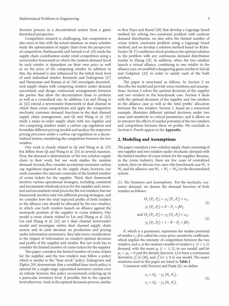
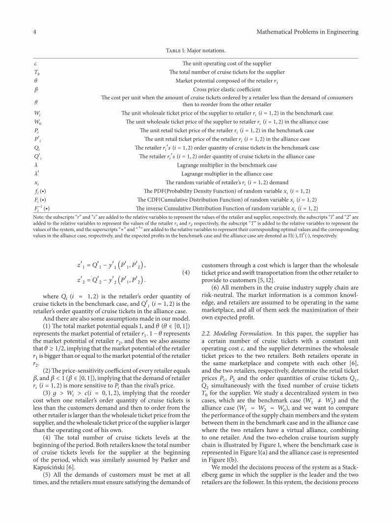
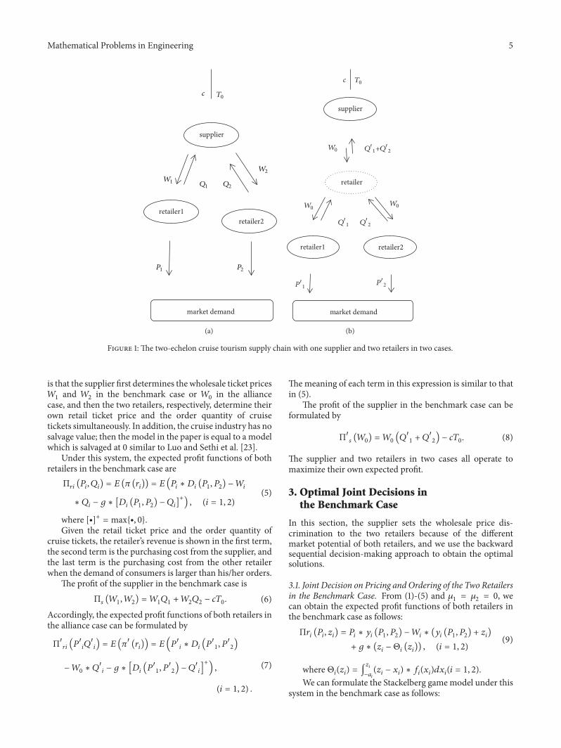
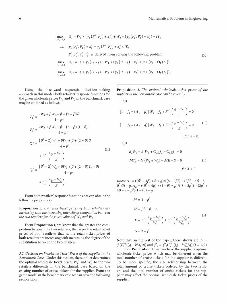
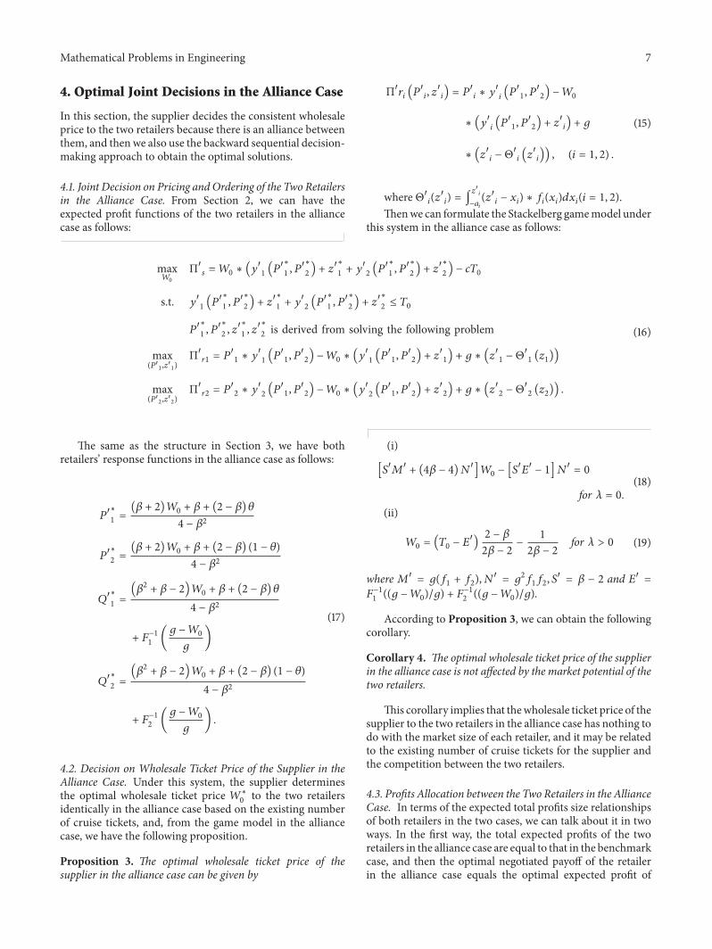
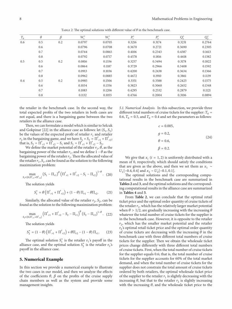
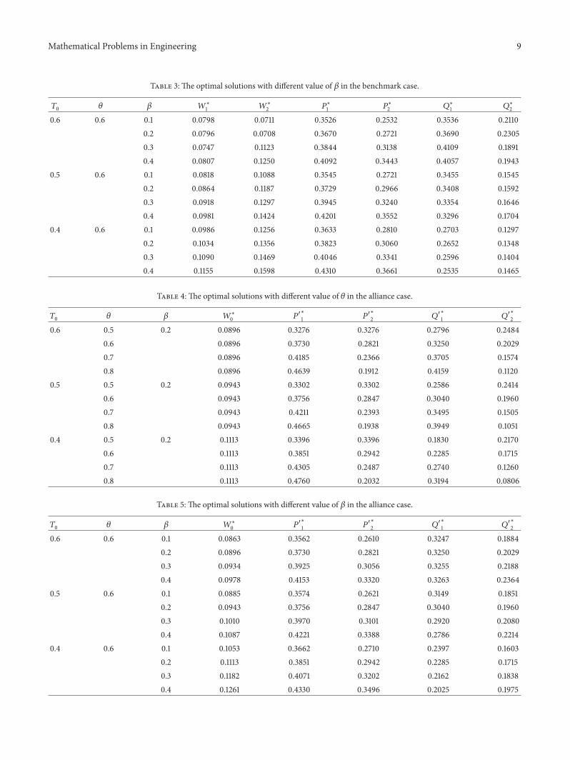
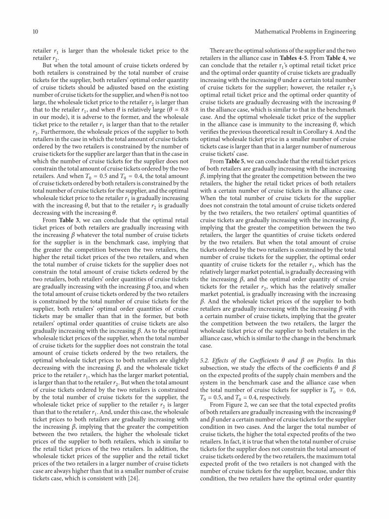
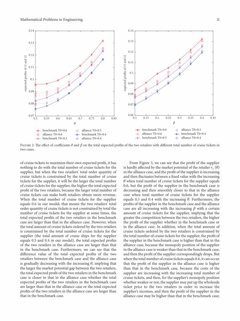
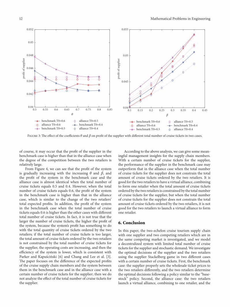
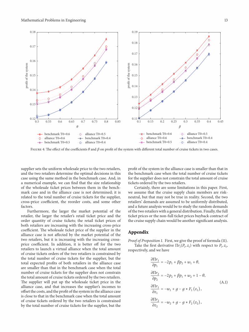
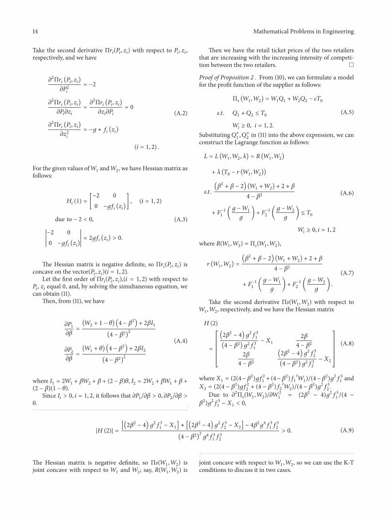
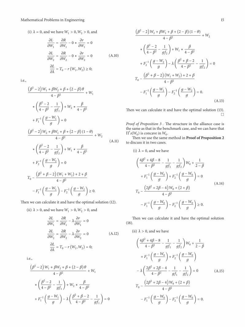

Hindawiwwwhindawicom Volume 2018
MathematicsJournal of
Hindawiwwwhindawicom Volume 2018
Mathematical Problems in Engineering
Applied MathematicsJournal of
Hindawiwwwhindawicom Volume 2018
Probability and StatisticsHindawiwwwhindawicom Volume 2018
Journal of
Hindawiwwwhindawicom Volume 2018
Mathematical PhysicsAdvances in
Complex AnalysisJournal of
Hindawiwwwhindawicom Volume 2018
OptimizationJournal of
Hindawiwwwhindawicom Volume 2018
Hindawiwwwhindawicom Volume 2018
Engineering Mathematics
International Journal of
Hindawiwwwhindawicom Volume 2018
Operations ResearchAdvances in
Journal of
Hindawiwwwhindawicom Volume 2018
Function SpacesAbstract and Applied AnalysisHindawiwwwhindawicom Volume 2018
International Journal of Mathematics and Mathematical Sciences
Hindawiwwwhindawicom Volume 2018
Hindawi Publishing Corporation httpwwwhindawicom Volume 2013Hindawiwwwhindawicom
The Scientific World Journal
Volume 2018
Hindawiwwwhindawicom Volume 2018Volume 2018
Numerical AnalysisNumerical AnalysisNumerical AnalysisNumerical AnalysisNumerical AnalysisNumerical AnalysisNumerical AnalysisNumerical AnalysisNumerical AnalysisNumerical AnalysisNumerical AnalysisNumerical AnalysisAdvances inAdvances in Discrete Dynamics in
Nature and SocietyHindawiwwwhindawicom Volume 2018
Hindawiwwwhindawicom
Dierential EquationsInternational Journal of
Volume 2018
Hindawiwwwhindawicom Volume 2018
Decision SciencesAdvances in
Hindawiwwwhindawicom Volume 2018
AnalysisInternational Journal of
Hindawiwwwhindawicom Volume 2018
Stochastic AnalysisInternational Journal of
Submit your manuscripts atwwwhindawicom