July 22, 1992 version.

Evolution of a Subsumption Architecture that Performs a Wall Following Task

for an Autonomous Mobile Robot via Genetic Programming

John R. Koza

Computer Science Department

Stanford University

Stanford, CA 94305 USA

E-MAIL: Koza@Sunburn.Stanford.Edu

PHONE: 415-941-0336 FAX: 415-941-9430

ABSTRACT

The goal in automatic programming is to get a computer to perform a task by telling it what

needs to be done, rather than by explicitly programming it. This paper considers the task of

automatically generating a computer program to enable an autonomous mobile robot to perform

the task of following the wall of an irregular shaped room. A human programmer has written

such a program in the style of the subsumption architecture. The solution produced by genetic

programming emerges as a result of Darwinian natural selection and genetic crossover (sexual

recombination) in a population of computer programs. This evolutionary process is driven by a

fitness measure which communicates the nature of the task to the computer.

1 Introduction and Overview

In the 1950s, Arthur Samuel identified the goal of getting a computer to perform a task without

being explicitly programmed as one of the central goals in the fields of computer science and

artificial intelligence. Such automatic programming of a computer involves merely telling the

computer what is to be done, rather than explicitly telling it, step-by-step, precisely how to

perform the desired task.

In this paper, we describe the conventional genetic algorithm (section 2) and the recently

developed genetic programming paradigm (section 3). We also describe the subsumption

architecture (section 4) and how a human programmer wrote a computer program, in the style of

the subsumption architecture, to control an autonomous mobile robot to perform the task of

following the wall of an irregular room (section 5).

We then show, in section 6, how genetic programming can be used to genetically breed a

computer program capable of controlling an autonomous mobile robot to perform the wall

following task. To do this, we use only the primitive robotic functions inherent in the wall

following problem, the sonar sensor inputs of the robot inherent in the problem, and a fitness

measure for ascertaining how well a given program performs the required task. The solution

produced by genetic programming emerges as a result of Darwinian natural selection and genetic

crossover (sexual recombination) in a population of computer programs. The learning process is

driven by the fitness measure.

2 Genetic Algorithms

John Holland's pioneering 1975 Adaptation in Natural and Artificial Systems described how the

evolutionary process in nature can be applied to artificial systems using the genetic algorithm

operating on fixed length character strings (Holland 1975). Holland demonstrated that a

population of fixed length character strings (each representing a proposed solution to a

problem) can be genetically bred using the Darwinian operation of fitness proportionate

reproduction and the genetic operation of recombination. The recombination operation

combines parts of two chromosome-like fixed length character strings, each selected on the basis

of their fitness, to produce new offspring strings. Holland established, among other things, that

the genetic algorithm is a mathematically near optimal approach to adaptation in that it

maximizes expected overall average payoff when the adaptive process is viewed as a multi-

armed slot machine problem requiring an optimal allocation of future trials given currently

available information.

Recent research on genetic algorithms can be found in Goldberg (1989), Davis (1991), and

Belew and Booker (1991).

3 Genetic Programming

For many problems, the most natural representation for solutions are computer programs. The

size, shape, and contents of the computer program to solve the problem is generally not known in

advance. The computer program that solves a given problem is typically a hierarchical

composition of various primitive functions and terminals. The desired program typically takes

the state variables or sensors of the system as its input and produces an external action as its

output.

The size and shape of the solution to the problem should be considered part of the answer

produced by a learning paradigm, not part of the question. It is unnatural and difficult to

represent program hierarchies whose size and shape must vary during the problem solving

process with the fixed length character strings generally used in the conventional genetic

algorithm.

In genetic programming, the individuals in the population are compositions of functions and

terminals appropriate to the particular problem domain. Depending on the particular problem at

hand, the set of functions used may include arithmetic operations, primitive robotic actions,

conditional branching operations, mathematical functions, or domain-specific functions.

The set of terminals used typically includes the sensor inputs or state variables appropriate to the

problem domain and possibly also includes various constants. The size and shape of the solution

is not specified in advance.

In genetic programming, one views the search for the solution to the problem at hand as a

search of the space of all possible compositions of functions and terminals (i.e. computer

programs) that can be recursively composed from the available functions and terminals.

The symbolic expressions (S-expressions) of the LISP programming language are an especially

convenient way to create and manipulate the compositions of functions and terminals described

above. These S-expressions in LISP correspond directly to the parse tree that is internally

created by most compilers.

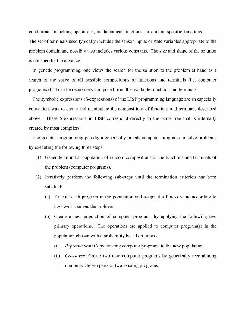
The genetic programming paradigm genetically breeds computer programs to solve problems

by executing the following three steps:

(1) Generate an initial population of random compositions of the functions and terminals of

the problem (computer programs).

(2) Iteratively perform the following sub-steps until the termination criterion has been

satisfied:

(a) Execute each program in the population and assign it a fitness value according to

how well it solves the problem.

(b) Create a new population of computer programs by applying the following two

primary operations. The operations are applied to computer program(s) in the

population chosen with a probability based on fitness.

(i) Reproduction: Copy existing computer programs to the new population.

(ii) Crossover: Create two new computer programs by genetically recombining

randomly chosen parts of two existing programs.

(3) The single best computer program in the population at the time of termination is

designated as the result. This result may be a solution (or approximate solution) to the

problem.

The basic genetic operations for the genetic programming paradigm are fitness proportionate

reproduction and crossover (recombination).

The reproduction operation copies individuals in the genetic population into the next

generation of the population in proportion to their fitness in grappling with the problem

environment. This operation is the basic engine of Darwinian survival and reproduction of the

fittest.

The crossover operation is a sexual operation that operates on two parental LISP S-expressions

and produces two offspring S-expressions using parts of each parent. The crossover operation

creates new offspring S-expressions by exchanging sub-trees (i.e. sub-lists) between the two par-

ents. Because entire sub-trees are swapped, this crossover operation always produces

syntactically and semantically valid LISP S-expressions as offspring regardless of the crossover

points.

For example, consider the two parental S-expressions:

(OR (NOT D1) (AND D0 D1))

(OR (OR D1 (NOT D0)) (AND (NOT D0) (NOT D1))

Figure 1 graphically depicts these two S-expressions as rooted, point-labeled trees with

ordered branches. The numbers on the tree are for reference only.

Assume that the points of both trees are numbered in a depth-first way starting at the left.

Suppose that point 2 (out of 6 points of the first parent) is randomly selected as the crossover

point for the first parent and that point 6 (out of 10 points of the second parent) is randomly

selected as the crossover point of the second parent. The crossover points in the trees above are

therefore the NOT in the first parent and the AND in the second parent.

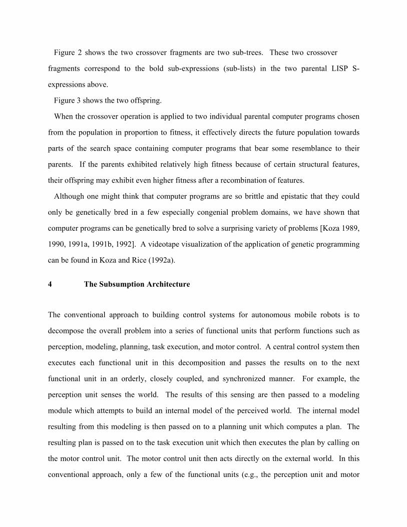
Figure 2 shows the two crossover fragments are two sub-trees. These two crossover

fragments correspond to the bold sub-expressions (sub-lists) in the two parental LISP S-

expressions above.

Figure 3 shows the two offspring.

When the crossover operation is applied to two individual parental computer programs chosen

from the population in proportion to fitness, it effectively directs the future population towards

parts of the search space containing computer programs that bear some resemblance to their

parents. If the parents exhibited relatively high fitness because of certain structural features,

their offspring may exhibit even higher fitness after a recombination of features.

Although one might think that computer programs are so brittle and epistatic that they could

only be genetically bred in a few especially congenial problem domains, we have shown that

computer programs can be genetically bred to solve a surprising variety of problems [Koza 1989,

1990, 1991a, 1991b, 1992]. A videotape visualization of the application of genetic programming

can be found in Koza and Rice (1992a).

4 The Subsumption Architecture

The conventional approach to building control systems for autonomous mobile robots is to

decompose the overall problem into a series of functional units that perform functions such as

perception, modeling, planning, task execution, and motor control. A central control system then

executes each functional unit in this decomposition and passes the results on to the next

functional unit in an orderly, closely coupled, and synchronized manner. For example, the

perception unit senses the world. The results of this sensing are then passed to a modeling

module which attempts to build an internal model of the perceived world. The internal model

resulting from this modeling is then passed on to a planning unit which computes a plan. The

resulting plan is passed on to the task execution unit which then executes the plan by calling on

the motor control unit. The motor control unit then acts directly on the external world. In this

conventional approach, only a few of the functional units (e.g., the perception unit and motor

control unit) typically are in direct communication with the world. The output of one

functional unit is tightly coupled to the next functional unit. One typically gets no performance

out of the system unless all the functional units are operating.

The subsumption architecture is an alternative to the conventional centrally controlled way of

building control systems for autonomous mobile robots which involves decomposing the

problem into a set of asynchronous task achieving behaviors (Brooks 1986, Brooks 1989,

Connell 1990). Overall control of the robot is achieved by the collective effect of the

asynchronous local interactions of the relatively primitive task achieving behaviors, each

communicating directly with the world and among themselves. In the subsumption architecture,

each task achieving behavior typically performs some low level function. For example, the task

achieving behaviors for an autonomous mobile robot might include tasks such as wandering,

exploring, identifying objects, avoiding objects, building maps, planning changes to the world,

monitoring changes to the world, and reasoning about behavior of the objects. The task

achieving behaviors operate locally and asynchronously and are only loosely coupled to one

another. Various subsets of the task achieving behaviors typically exhibit some partial

competence in solving the problem.

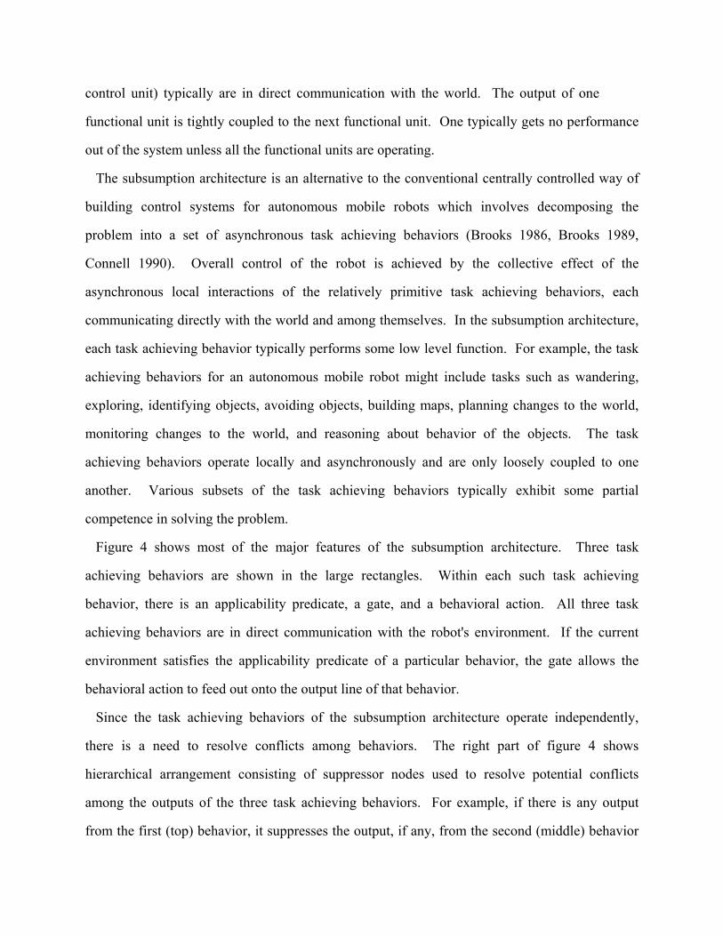
Figure 4 shows most of the major features of the subsumption architecture. Three task

achieving behaviors are shown in the large rectangles. Within each such task achieving

behavior, there is an applicability predicate, a gate, and a behavioral action. All three task

achieving behaviors are in direct communication with the robot's environment. If the current

environment satisfies the applicability predicate of a particular behavior, the gate allows the

behavioral action to feed out onto the output line of that behavior.

Since the task achieving behaviors of the subsumption architecture operate independently,

there is a need to resolve conflicts among behaviors. The right part of figure 4 shows

hierarchical arrangement consisting of suppressor nodes used to resolve potential conflicts

among the outputs of the three task achieving behaviors. For example, if there is any output

from the first (top) behavior, it suppresses the output, if any, from the second (middle) behavior

at suppressor node A. Note that figure 4 does not show the alarm clock timers of the

augmented finite state machines of the subsumption architecture (Brooks 1986, 1989) which

allow a variable to be set to a certain value (i.e., state) for a prescribed period of time. S

The applicability predicate of each behavior in the subsumption architecture consists of some

composition (ultimately returning either T or NIL) of conditional logical functions and

environmental input sensors. The action part of each behavior typically consists of some

composition of functions taking some actions. The hierarchical arrangement of suppressor nodes

operating on the emitted actions of the behaviors consists of a composition of logical functions

(returning either an emitted action or NIL).

One can reformulate the role of the three applicability predicates and the suppressor nodes

shown in figure 4 as the following composition of ordinary if-then conditional functions:

(IF A-P-1 BEHAVIOR-1

(IF A-P-2 BEHAVIOR-2

(IF A-P-3 BEHAVIOR-3))),

where the three-argument IF operator in the above executes its second argument if its first

argument evaluates to T (true), but otherwise executes its third argument.

This reformulation makes clear that the cumulative effect of the roles of the applicability

predicates and suppressor nodes of the subsumption architecture is equivalent to a composition

of ordinary conditional if-then-else functions.

Considerable ingenuity and skill on the part of a human programmer are required in order to

conceive and write a composition of task achieving behaviors that are actually able to solve a

particular problem in the style of the subsumption architecture.

The question arises as to whether it is possible to evolve a subsumption architecture to solve

problems.

5 TOTO, the Wall Following Robot

Mataric 1990 has implemented the subsumption architecture by conceiving and writing a set of

four LISP computer programs for performing four task achieving behaviors which together

enable an autonomous mobile robot called TOTO to follow the walls in an irregular room.

Figure 5 shows a robot at point (12, 16) near the center of an irregularly shaped room.

TOTO has 12 sonar sensors, each covering a 30° sector, which report the distance to the

nearest wall as a floating-point number in feet and a sensor called STOPPED to indicate if the

robot is stopped against the wall.

Mataric's robot was capable of executing five primitive motor functions, namely moving

forward (MF) by a constant distance of 1.0 foot, moving backward (MB) by 1.33 feet distance,

turning right (TR) (i.e. clockwise) by 30°, turning left (TL) by 30°, and stopping (STOP).

The sensors and primitive motor functions are not labeled, ordered, or interpreted in any way.

The robot does not know a priori what the sensors mean nor what the primitive motor functions

do.

In addition, three constant parameters are associated with the problem. The edging distance

(EDG) representing the preferred distance between the robot and the wall was 2.3 feet. The

minimum safe distance (MSD) between the robot and the wall was 2.0 feet. The danger zone

(DZ) was 1.0 feet.

The 13 sensor values, five primitive motor functions, and three constant parameters just

described are a given part of the statement of the wall following problem.

In what follows, we show how the wall following problem was solved by a human programmer

using the subsumption architecture and we then show how the wall following problem can be

solved by means of genetic programming.

Mataric's four LISP programs (called STROLL, AVOID, ALIGN, and CORRECT) correspond

to task achieving behaviors which she conceived and wrote. Various subsets of these four task

achieving behaviors exhibit some partial competence in solving part of the overall problem. For

example, the robot becomes capable of collision-free wandering with only the STROLL

and AVOID behaviors. The robot becomes capable of tracing convex boundaries with the

addition of the ALIGN behavior to these first two behaviors. Finally, the robot becomes capable

of general boundary tracing with the further addition of the CORRECT behavior.

Mataric's four LISP programs also contained nine atoms defined in terms of the given sonar

sensors (e.g., the dynamically computed minimum of various subsets of sonar sensors and SS,

the dynamically computed minimum of all sonar sensors). Mataric's four LISP programs also

contained nine additional LISP functions, namely IF, AND, NOT, COND, >, >=, =, <=, and >.

In total, Mataric's four LISP programs contained 25 different atoms and 14 different functions

and consisted of 151 points (i.e., atoms and functions).

The fact that Mataric was able to conceive and write her four programs is significant evidence

(based on this one problem) for one of the claims of the subsumption architecture, namely that it

is possible to build a control system for an autonomous mobile robot using loosely coupled,

asynchronous task achieving behaviors. Mataric's four programs are very different from the

conventional tightly controlled and synchronized approach to robotic control in that they did not

contain a specific, identifiable perception unit, a modeling unit, a planning unit, a task execution

unit, or a motor control unit.

6 Applying Genetic Programming to the Wall Following Problem

There are five major steps in preparing to use genetic programming, namely, determining: (1) the

set of terminals, (2) the set of functions, (3) the fitness function, (4) the parameters and variables

for controlling the run, and (5) the criterion for designating a result and terminating a run.

Learning, in general, requires some experimentation in order to obtain the information needed

by the learning algorithm to find the solution to the problem. Since learning here would require

that the robot perform the overall task a certain large number of times, we planned to simulate

the activities of the robot, rather than use a physical robot such as TOTO. Since our simulated

robot was not intended to ever stop and could not, in any event, be damaged by running into a

wall, we had no use for the STOP function, the STOPPED sensor, or the danger zone

parameter DZ. In our simulations, we let our robot push up against the wall, and, if no change of

state occurred after an additional time step, the robot was viewed as having stopped and that

particular simulation ended.

We retained Mataric's other two constant parameters MSD and EDG.

The four primitive motor functions MF, MB, TR, and TL each take one time step (i.e., 1.0

seconds) to execute. All sonar distances are dynamically recomputed after each execution of a

move or turn.

The first major step in preparing to use genetic programming is to identify the set of terminals.

Our terminal set T for this problem consists of the 12 given sonar sensors, two given constant

parameters, the combined parameter SS, and four of Mataric's five primitive motor functions as

follows:

T = {S00, S01, S02, S03, ... , S11, MSD, EDG, SS, (MF), (MB), (TR), (TL)}.

Thus, at each time step, our simulated robot has access to 15 floating-point values.

The second major step in preparing to use genetic programming is to identify the function set.

Human programmers usually find it convenient to use a variety of different functions (such as IF,

AND, NOT, COND, >, >=, =, <=, and >) in writing computer programs. Although not

necessary, we chose to simplify the set of available functions in genetic programming. All of the

numerical comparisons that Mataric could perform using >, >=, =, <=, and > can be performed

using a single comparison such as the <= comparison (i.e. less than or equal). As previously

mentioned, a subsumption architecture consisting of various task achieving behaviors (each with

an applicability predicate) and a network of suppressor nodes to resolve conflicts can be

reformulated as a composition of ordinary if-then conditional functions. For simplicity, we used

the IFLTE conditional comparison operator taking four arguments in our function set. If the

value of the first argument is less than or equal the value of the second argument, the third

argument is evaluated and returned. Otherwise, the fourth argument is evaluated and returned.

Since the terminals in this problem take on floating-point values, this function is used to

compare values of the terminals. The IFLTE operator allows alternative actions to be executed

based on comparisons of observation from the robot's environment. It allows, among other

things, a particular action to be executed based on the robot's current environment. It allows one

action to suppress another. It allows for the computation of the minimum of a subset of two or

more sensors. The IFLTE operator is implemented as a macro in Common LISP. The

connective function PROGN2 taking two arguments evaluates both of its arguments, in

sequence.

Thus, our function set F for this problem consisted of

F = {IFLTE, PROGN2}.

Although the primary functionality of the moving and turning functions lies in their side

effects on the state of the robot, it is necessary, in order to have closure, that these functions

return some numerical value. For the first of the two ways we approached this problem (i.e.,

Example 1), we decided that each of the four moving and turning functions would return the

minimum of the two distances reported by the two sensors that look in the direction of forward

movement (i.e., S02 representing the 11:30 o'clock direction and S03 representing the 12:30

o'clock direction).

The search space for a run of genetic programming consists of the space of all possible

compositions of functions and terminals (i.e. computer programs) that can be recursively com-

posed from the available functions from the function set and the available terminals from the

terminal set. This search space is clearly enormous for this problem.

The third major step in preparing to use genetic programming is the determination of the

fitness measure. A human programmer, of course, uses human intelligence to write a computer

program. In contrast, genetic programming is guided by the pressure exerted by the fitness

measure and natural selection.

A wall following robot may be viewed as a robot that travels along the entire perimeter

of the irregularly shaped room. Raw fitness can be the portion of the perimeter which is

traversed by the robot within some reasonable amount of time. Noting that Mataric's edging

distance was 2.3 feet, we visualized placing contiguous 2.3 foot square tiles along the perimeter

of the room. Twelve such tiles fit along the 27.6 foot north wall and 12 such tiles fit along the

27.6 foot west wall. In all, a total of 56 tiles are required to cover the entire periphery of the

irregular room.

Figure 6 shows the irregular room with the 56 tiles (each with a heavy dot at its center) along

its periphery. Mataric's four LISP programs take 203 time steps to travel onto each of the 56

tiles. We established a time frame for this problem by allowing approximately twice Mataric's

203 time steps. Specifically, we defined raw fitness to be the number (from 0 to 56) of tiles that

are touched by the robot within 400 time steps. If a robot travels onto each of these 56 tiles

within 400 time steps, we will regard it as being successful in doing wall following.

Standardized fitness is 56 minus raw fitness.

The fourth major step in preparing to use genetic programming is selecting the values of

certain parameters. The major parameters for controlling a run of genetic programming are the

population size and the number of generations to be run. The population size is 1,000 here and a

maximum of 101 generations is established for each run.

In addition to the above two major parameters, each run of genetic programming is controlled

by a number of minor parameters. In particular, each new generation is created from the

preceding generation by applying the reproduction operation to 10% of the population and by

applying the crossover operation to 90% of the population (with both parents selected with a

probability proportional to fitness). In selecting crossover points, 90% were internal (function)

points of the tree and 10% were external (terminal) points of the tree. For the practical reason of

conserving computer time, the depth of initial random S-expressions was limited to 6 and the

depth of S-expressions created by crossover was limited to 17. The individuals in the initial

random generation were generated so as to obtain a wide variety of different sizes and shapes

among the S-expressions. Fitness is "adjusted" to emphasize small differences near zero.

See Koza (1992) for a detailed explanation of these parameters.

Finally, the fifth major step in preparing to use genetic programming is the selection of the

criterion for terminating a run and accepting a result. We will terminate a given run when either

(i) genetic programming produces a computer program which scores a raw fitness of 56, or (ii)

101 generations have been run. In genetic programming, both the average fitness of the

population as a whole and the fitness of the best-of-generation individual generally improve

from generation to generation. The best-so-far individual obtained in any generation will be

designated as the result of a run of genetic programming.

6.1 Example 1

As one would expect, the individual S-expressions in the initial population of randomly created

computer programs are highly unfit in solving the problem. In one run of Example 1 of the wall

following problem, 57% of the individuals in the population in the generation 0 scored a raw

fitness of zero. Many of this group of zero-scoring S-expressions merely cause the robot to turn

without ever moving from its initial location near the center of the room.

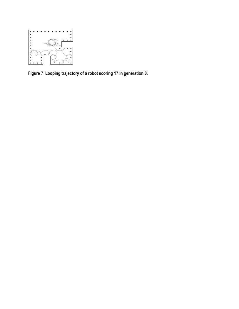
Other individuals scoring zero in generation 0 actually move, but merely wander aimlessly and

never even reach the wall. Figure 7 shows such an aimless wanderer.

About 20% of the individuals in generation 0 score one out of a possible 56 by heading into a

wall (thereby touching one tile on the periphery of the room) and then continuing to

unconditionally push itself up against the wall. About 7% scored two (out of 56) and another

15% of the population scored between 3 and 10.

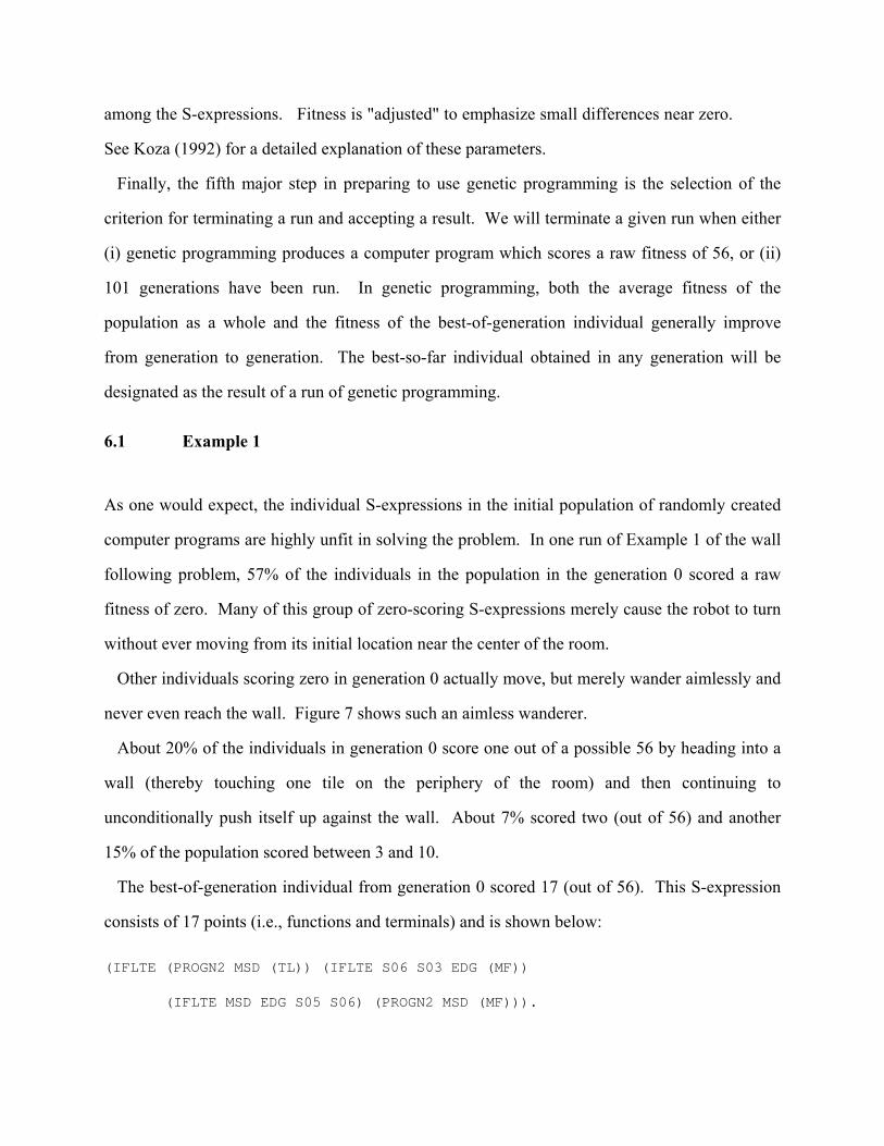
The best-of-generation individual from generation 0 scored 17 (out of 56). This S-expression

consists of 17 points (i.e., functions and terminals) and is shown below:

(IFLTE (PROGN2 MSD (TL)) (IFLTE S06 S03 EDG (MF))

(IFLTE MSD EDG S05 S06) (PROGN2 MSD (MF))).

Figure 7 shows the looping trajectory of the robot while executing the best-of-

generation program for generation 0. As can be seen, the robot starts in the middle of the room

and loops around itself three times and then bumps into the protrusion from the east wall. The

robot then begins a series of 11 loops which cause it to repeatedly hit the wall at irregular

intervals and which leaves many intervening points along the wall untouched. This individual

times out on the west wall at 400 time steps without ever having even traveled to the northern

part of the room. The 39 heavy dots around the edges of the room represent the 39 tiles that

were not touched by the robot before it timed out after 400 time steps.

Even in this initial random generation, some individuals are somewhat more fit than others.

The best-of-generation looping individual from generation 0 is far from perfect; however, it is

considerably better than the non-moving individuals, the aimless wandering individuals, and the

wall-banging individuals. The Darwinian operation of fitness proportionate reproduction and

genetic crossover (sexual recombination) is applied to the population, and a new generation of S-

expressions is produced.

Figure 8 shows the ricocheting trajectory of the robot while executing the best-of-generation

program for generation 2 which scored 27 and consisted of 57 points. As can be seen, the robot

ricochets around the room 16 times and, more or less accidentally, touches occasional points on

the periphery of the room.

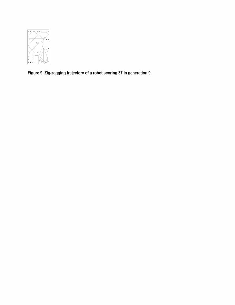
Figure 9 shows the zig-zagging trajectory of the robot while executing the best-of-generation

program for generation 9 which scored 37 and consisted of 97 points. This individual wastes

considerable time by making numerous trips across the middle of the room. This trajectory

misses several contiguous groups of tiles as well as several corner tiles.

None of the foregoing behavior can be characterized as wall following. However, by

generation 14, the best-of-generation S-expression scored 49 and consisted of 45 points. Figure

10 shows the trajectory of the robot while executing this best-of-generation program for

generation 14. This individual does exhibit approximate wall following behavior. After once

reaching a wall, the robot makes broad snake like motions along the walls and never returns to

the middle of the room. This individual misses two points along the straight portions of

the walls, four concave corners, and one convex corner.

By generation 49, the best-of-generation S-expression scored 55 and consisted of 157 points.

Figure 11 shows the slithering trajectory of the robot while executing this best-of-generation

program for generation 49. The robot follows the wall rather closely and misses only one point

in the upper right corner. It scores 55 out of 56.

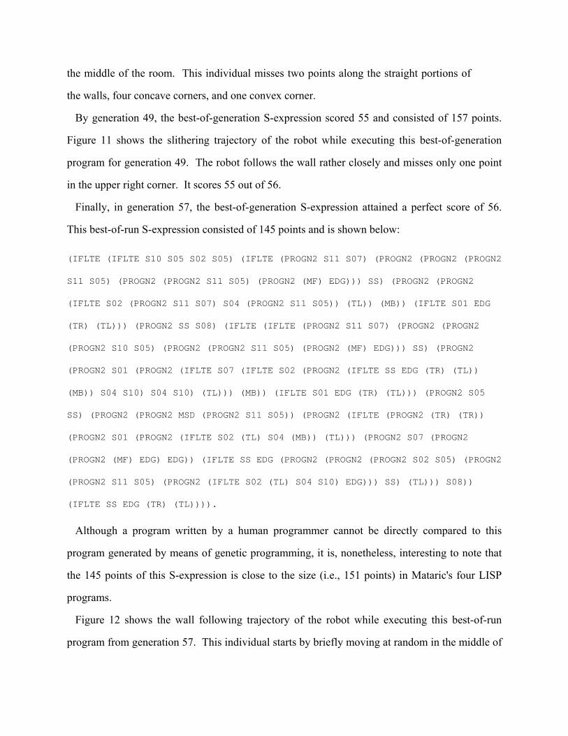
Finally, in generation 57, the best-of-generation S-expression attained a perfect score of 56.

This best-of-run S-expression consisted of 145 points and is shown below:

(IFLTE (IFLTE S10 S05 S02 S05) (IFLTE (PROGN2 S11 S07) (PROGN2 (PROGN2 (PROGN2

S11 S05) (PROGN2 (PROGN2 S11 S05) (PROGN2 (MF) EDG))) SS) (PROGN2 (PROGN2

(IFLTE S02 (PROGN2 S11 S07) S04 (PROGN2 S11 S05)) (TL)) (MB)) (IFLTE S01 EDG

(TR) (TL))) (PROGN2 SS S08) (IFLTE (IFLTE (PROGN2 S11 S07) (PROGN2 (PROGN2

(PROGN2 S10 S05) (PROGN2 (PROGN2 S11 S05) (PROGN2 (MF) EDG))) SS) (PROGN2

(PROGN2 S01 (PROGN2 (IFLTE S07 (IFLTE S02 (PROGN2 (IFLTE SS EDG (TR) (TL))

(MB)) S04 S10) S04 S10) (TL))) (MB)) (IFLTE S01 EDG (TR) (TL))) (PROGN2 S05

SS) (PROGN2 (PROGN2 MSD (PROGN2 S11 S05)) (PROGN2 (IFLTE (PROGN2 (TR) (TR))

(PROGN2 S01 (PROGN2 (IFLTE S02 (TL) S04 (MB)) (TL))) (PROGN2 S07 (PROGN2

(PROGN2 (MF) EDG) EDG)) (IFLTE SS EDG (PROGN2 (PROGN2 (PROGN2 S02 S05) (PROGN2

(PROGN2 S11 S05) (PROGN2 (IFLTE S02 (TL) S04 S10) EDG))) SS) (TL))) S08))

(IFLTE SS EDG (TR) (TL)))).

Although a program written by a human programmer cannot be directly compared to this

program generated by means of genetic programming, it is, nonetheless, interesting to note that

the 145 points of this S-expression is close to the size (i.e., 151 points) in Mataric's four LISP

programs.

Figure 12 shows the wall following trajectory of the robot while executing this best-of-run

program from generation 57. This individual starts by briefly moving at random in the middle of

the room. However, as soon as it reaches the wall, it moves along the wall. It stays much

closer to the wall than the slithering trajectory from generation 49 and it touches 100% of the 56

tiles along the periphery of the room. This individuals takes 395 time steps to touch all 56 tiles.

Figure 13 shows, by generation, the average standardized fitness of the population as a whole

and the value of standardized fitness for the best-of-generation individual. Note that the

improvement in fitness from generation to generation is progressive and does not involve great

leaps.

Figure 14 shows the hits histograms for generations 0, 6, 18, 30 and 57. Notice the undulating

left-to-right "slinky" movement of the histogram as the population as a whole progressively

improves.

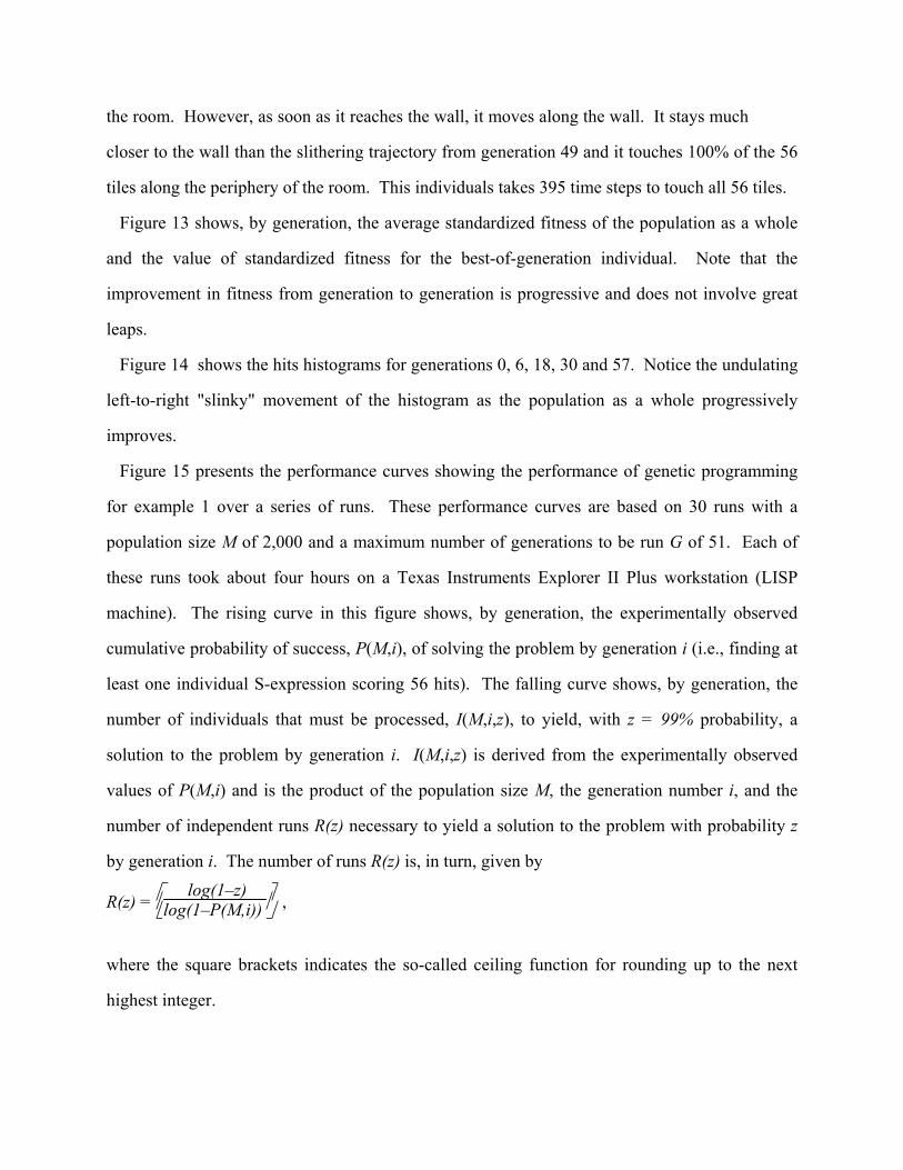
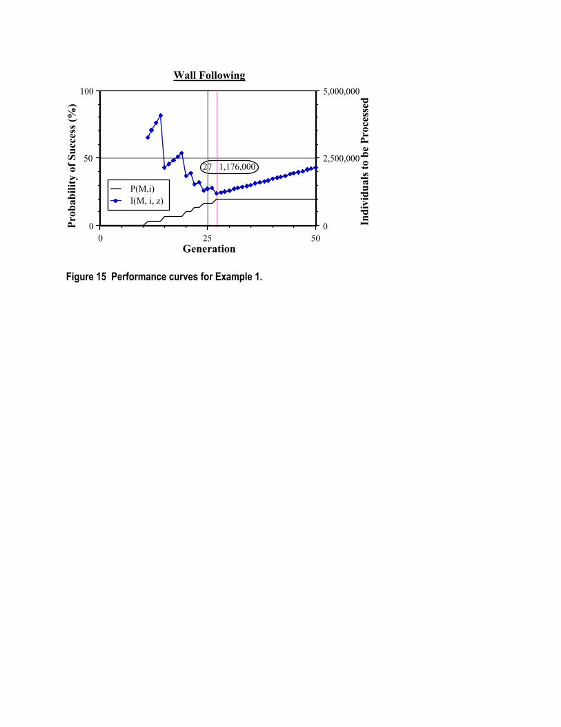
Figure 15 presents the performance curves showing the performance of genetic programming

for example 1 over a series of runs. These performance curves are based on 30 runs with a

population size M of 2,000 and a maximum number of generations to be run G of 51. Each of

these runs took about four hours on a Texas Instruments Explorer II Plus workstation (LISP

machine). The rising curve in this figure shows, by generation, the experimentally observed

cumulative probability of success, P(M,i), of solving the problem by generation i (i.e., finding at

least one individual S-expression scoring 56 hits). The falling curve shows, by generation, the

number of individuals that must be processed, I(M,i,z), to yield, with z = 99% probability, a

solution to the problem by generation i. I(M,i,z) is derived from the experimentally observed

values of P(M,i) and is the product of the population size M, the generation number i, and the

number of independent runs R(z) necessary to yield a solution to the problem with probability z

by generation i. The number of runs R(z) is, in turn, given by

R(z) =

log(1–z)

log(1–P(M,i)) ,

where the square brackets indicates the so-called ceiling function for rounding up to the next

highest integer.

As can be seen in figure 15, the experimentally observed value of the cumulative

probability of success, P(M,i), is 20% by generation 27. The I(M,i,z) curve reaches a minimum

value at generation 27 (highlighted by the light dotted vertical line). For a value of P(M,i) of

20%, the number of runs R(z) is 21. The two numbers in the oval indicate that if this problem is

run through to generation 27, processing a total of 1,176,000 individuals (i.e., 2,000 times 28

generations times 21 runs) is sufficient to yield a solution of this problem with 99% probability.

This number 1,176,000 is a measure of the computational effort necessary to solve this problem

with 99% probability. See Koza 1992 for details.

6.2 Example 2

In the foregoing discussion of the wall following problem, the search for a solution to the wall

following problem was facilitated by the presence of the sensor SS in the terminal set and the

fact that the functions MF, MB, TL, and TR returned a numerical value equal to the minimum of

several designated sensors.

The wall following problem can also be solved without the terminal SS and with the four

functions each returning a constant value of zero. We call these four new functions MF0, MB0,

TL0, and TR0. The new function set is

F0 = {MF0, MB0, TR0, TL0, IFLTE, PROGN2}

Figure 16 shows, by generation, for Example 2 of the wall following problem with the new

function set F0, the progressive improvement in the average standardized fitness of the

population as a whole and the value of standardized fitness for the best-of-generation individual

and the worst-of-generation individual.

In generation 102 of one run with function set F0, we obtained the following S-expression with

237 points which scored 56 out of 56 within the allowed time.

(PROGN2 (PROGN2 (PROGN2 (PROGN2 (IFLTE S06 S10 S09 S09) (PROGN2 EDG

(MB0))) (IFLTE (IFLTE S08 MSD MSD S05) S09 (PROGN2 S07 (MB0)) (PROGN2 (PROGN2

(PROGN2 (IFLTE S06 S10 S04 S09) (IFLTE S09 S09 S05 MSD)) (IFLTE (IFLTE S08 MSD

MSD S05) (PROGN2 S00 S10) (PROGN2 S07 (IFLTE (MF0) S05 (TR0) (MB0))) (PROGN2

(IFLTE (MF0) S05 (TR0) (PROGN2 S00 S10)) (PROGN2 (TR0) S05)))) (MB0)))) (MB0))

(IFLTE (PROGN2 (IFLTE S00 S07 S01 (MB0)) (PROGN2 (IFLTE S00 S07 S01 (MB0))

(PROGN2 (PROGN2 MSD (TL0)) (PROGN2 S04 S09)))) (PROGN2 (IFLTE S07 EDG S03 S06)

(IFLTE S09 S09 S05 S05)) (PROGN2 (PROGN2 (IFLTE (MF0) S05 (TR0) (IFLTE (IFLTE

(TL0) S08 S01 (MF0)) (PROGN2 S03 S07) (PROGN2 (PROGN2 (IFLTE S06 S10 S04 S09)

(PROGN2 S07 (MB0))) (IFLTE (PROGN2 (PROGN2 S07 (IFLTE (MF0) S05 (TR0) (MB0)))

(IFLTE (PROGN2 (TL0) S00) (TR0) (IFLTE S01 S00 S04 (TR0)) (IFLTE S00 S07 S01

(IFLTE (IFLTE S07 EDG S03 S06) S01 (IFLTE S11 S08 S11 S05) (TR0))))) (PROGN2

S00 S10) (PROGN2 S07 (MB0)) (PROGN2 (PROGN2 (PROGN2 (IFLTE S06 S10 S04 S09)

(IFLTE S09 S09 S00 MSD)) (IFLTE (IFLTE (PROGN2 S03 (MB0)) S08 S01 (MF0))

(PROGN2 S00 S10) (IFLTE S06 S10 S04 S09) (PROGN2 (IFLTE (MF0) S05 (TR0) (MB0))

(IFLTE S09 S09 S05 S05)))) (MB0)))) (IFLTE S00 S07 (MB0) (TR0)))) (PROGN2

(TR0) S04)) (MB0)) (PROGN2 (PROGN2 (TL0) (MB0)) (IFLTE (PROGN2 (TL0) S00)

(IFLTE S08 MSD MSD S05) (PROGN2 (PROGN2 S07 (MB0)) S05) (IFLTE S00 S07 S01

(PROGN2 S04 S09)))))).

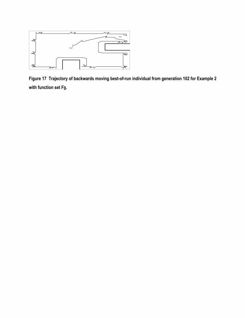
Figure 17 shows the trajectory of the robot executing this best-of-run individual from

generation 102 for the wall following problem with the function set F0. Interestingly, this

individual causes the robot to move backwards as it follows the wall (thereby taking advantage

of the speed advantage in Mataric's MB operator).

This S-expression simplifies to the following S-expression with 58 points (the numbers at the

left being line numbers for reference purposes only):

1 (PROGN

2 (MB)

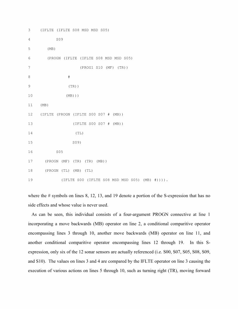
3 (IFLTE (IFLTE S08 MSD MSD S05)

4 S09

5 (MB)

6 (PROGN (IFLTE (IFLTE S08 MSD MSD S05)

7 (PROG1 S10 (MF) (TR))

8 #

9 (TR))

10 (MB)))

11 (MB)

12 (IFLTE (PROGN (IFLTE S00 S07 # (MB))

13 (IFLTE S00 S07 # (MB))

14 (TL)

15 S09)

16 S05

17 (PROGN (MF) (TR) (TR) (MB))

18 (PROGN (TL) (MB) (TL)

19 (IFLTE S00 (IFLTE S08 MSD MSD S05) (MB) #)))).

where the # symbols on lines 8, 12, 13, and 19 denote a portion of the S-expression that has no

side effects and whose value is never used.

As can be seen, this individual consists of a four-argument PROGN connective at line 1

incorporating a move backwards (MB) operator on line 2, a conditional comparitive operator

encompassing lines 3 through 10, another move backwards (MB) operator on line 11, and

another conditional comparitive operator encompassing lines 12 through 19. In this S-

expression, only six of the 12 sonar sensors are actually referenced (i.e. S00, S07, S05, S08, S09,

and S10). The values on lines 3 and 4 are compared by the IFLTE operator on line 3 causing the

execution of various actions on lines 5 through 10, such as turning right (TR), moving forward

(MF), and moving backwards (MB). The values of lines 15 and 16 are compared by the

IFLTE operator on line 12 and either the four actions on line 17 or the actions on lines 18 and 19

are executed.

We similarly evolved a computer program to perform the box moving task (Koza and Rice

1992b) and compared genetic programming to reinforcement learning techniques. The behavior

of computer programs that perform both the wall following task described in this paper and the

box moving task can be seen on videotape (Koza and Rice 1992a).

7 Conclusion

We used genetic programming to genetically breed, in two ways, a computer program that

enables an autonomous mobile robot to follow a wall in an irregular room.

8 Acknowledgements

James P. Rice of the Knowledge Systems Laboratory at Stanford University made numerous

contributions in connection with the computer programming of the above.

9 References

Belew, Richard and Booker, Lashon (editors) Proceedings of the Fourth International

Conference on Genetic Algorithms. San Mateo, CA: Morgan Kaufmann Publishers Inc.

1991.

Brooks, Rodney. A robust layered control system for a mobile robot. IEEE Journal of Robotics

and Automation. 2(1) March 1986.

Brooks, Rodney. A robot that walks: emergent behaviors from a carefully evolved network.

Neural Computation 1(2), 253-262. 1989.

Connell, J. Minimalist Mobile Robotics. Boston, MA: Academic Press 1990.

Davis, Lawrence. Handbook of Genetic Algorithms. New York: Van Nostrand Reinhold.1991.

Goldberg, David E. Genetic Algorithms in Search, Optimization, and Machine Learning.

Reading, MA: Addison-Wesley l989.

Holland, John H. Adaptation in Natural and Artificial Systems. Ann Arbor, MI: University of

Michigan Press 1975. Revised edition available from The MIT Press 1992.

Koza, John R. Hierarchical genetic algorithms operating on populations of computer programs."

In Proceedings of the 11th International Joint Conference on Artificial Intelligence. San

Mateo, CA: Morgan Kaufman 1989. Pages 768-774.

Koza, John R. Genetic Programming: A Paradigm for Genetically Breeding Populations of

Computer Programs to Solve Problems. Stanford University Computer Science

Department Technical Report STAN-CS-90-1314. June 1990.

Koza, John R. 1991a. Genetic evolution and co-evolution of computer programs. In Langton,

Christopher, Taylor, Charles, Farmer, J. Doyne, and Rasmussen, Steen (editors). Artificial

Life II, SFI Studies in the Sciences of Complexity. Volume X. Redwood City, CA: Addison-

Wesley 1991. 603-629. .

Koza, John R. 1991b. Evolution and co-evolution of computer programs to control independent-

acting agents. In Meyer, Jean-Arcady and Wilson, Stewart W. From Animals to Animats:

Proceedings of the First International Conference on Simulation of Adaptive Behavior.

Paris. September 24-28, 1990. Cambridge, MA: The MIT Press 1991.

Koza, John R. Genetic Programming: On the Programming of Computers by Means of Natural

Selection. Cambridge, MA: The MIT Press 1992.

Koza, John R., and Rice, James P. 1992a. Genetic Programming: The Movie. Cambridge, MA:

The MIT Press 1992. 1992a.

Koza, John R., and Rice, James P. 1992b. Automatic programming of robots using genetic

programming. In Proceedings of Tenth National Conference on Artificial Intelligence.

Menlo Park, CA: AAAI Press / The MIT Press 1992. Pages 194-201. 1992b.

Mataric, Maja J. A Distributed Model for Mobile Robot Environment-Learning and

Navigation. Massachusetts Institute of Technology Artificial Intelligence Laboratory

technical report AI-TR-1228. May 1990.

OR

NOT AND

D0 D1D1 D1

OR

ANDOR

NOT

D0

NOT NOT

D0 D1

2

3

4

5 6

1

2

3

1

4

5

6

7

8

9

10

Figure 1 Two parental computer programs shown as trees with ordered branches.

NOT

D1

AND

NOT NOT

D0 D1

Figure 2 The two crossover fragments.

OR

AND

NOT NOT

D0 D1

AND

D0 D1

NOT

OR

NOT

D0

D1 D1

OR

Figure 3 Offspring resulting from crossover.

Output

Suppressor Node A

Suppressor Node B

Input from Robot's

Environment

Applicability Predicate 1

Behavior 1 Gate

Applicability Predicate 2

Behavior 2 Gate

Applicability Predicate 3

Behavior 3 Gate

Figure 4 Subsumption architecture with three task achieving behaviors.

S00 = 12.4

S01 = 16.4 S02 = 12.0 S03 = 12.0 S04 = 16.4

S05 = 9.0

S06 = 16.2

S07 = 22.1S08 = 16.6

S09 = 9.4

S10 = 17.0

S11 = 12.4

Figure 5 Robot with 12 sonar sensors located near middle of an irregular room.

Start

End

Start

End

Figure 6 Aimless wandering trajectory of a robot (scoring zero) from generation 0.

Start

End

Figure 7 Looping trajectory of a robot scoring 17 in generation 0.

Start

End

Figure 8 Ricocheting trajectory of a robot scoring 27 in generation 2.

Start

End

Figure 9 Zig-zagging trajectory of a robot scoring 37 in generation 9.

End

Start

Figure 10 Broad snake like trajectory of a robot scoring 49 in generation 14.

End

Start

Figure 11 Slithering trajectory of a robot scoring 55 out of 56 in generation 49.

Start

End

Figure 12 Wall following trajectory of a best-of-run individual from generation 57 for Example 1.

0 29 580

14

28

42

56

Worst of Gen.AverageBest of Gen.

Wall Following — Best of Gen., Worst and Average

Generation

Stan

dard

ized

Fitn

ess

Figure 13 Standardized fitness for Example 1.

0 28 560

200400600800

1000Wall Following — Generation 0

Hits

Freq

uenc

y

0 28 560

200400600800

1000Wall Following — Generation 6

Hits

Freq

uenc

y

0 28 560

200400600800

1000Wall Following — Generation 18

Hits

Freq

uenc

y

0 28 560

200400600800

1000Wall Following — Generation 30

Hits

Freq

uenc

y

0 28 560

200400600800

1000Wall Following — Generation 57

Hits

Freq

uenc

y

Figure 14 Hits histogram for generations 0, 6, 18, 30 and 57 for Example 1.

27 1,176,000

0 25 500

50

100

0

2,500,000

5,000,000

P(M,i)I(M, i, z)

Wall Following

Generation

Prob

abili

ty o

f Suc

cess

(%)

Indi

vidu

als t

o be

Pro

cess

ed

Figure 15 Performance curves for Example 1.

0 51 1020

14

28

42

56

Worst of Gen.AverageBest of Gen.

Wall Following — Best of Gen., Worst and Average

Generation

Stan

dard

ized

Fitn

ess

Figure 16 Standardized fitness for Example 2 with function set F0.

Start

End

Figure 17 Trajectory of backwards moving best-of-run individual from generation 102 for Example 2

with function set F0.