Embed Size (px)
Citation preview
A Work Project, presented as part of the requirements for the Award of a Master Degree in Finance from the NOVA – School of Business and Economics.
THE IMPACT OF DEDOLLARIZATION IN THE ANGOLAN BANKING SECTOR BANCO DE FOMENTO DE ANGOLA CASESTUDY
JOÃO RICARDO CORREIA DA SILVEIRA CATANA 24873
A Project carried out on the Master in Finance Program, under the supervision of: Professor Francesco Franco
January the 6th of 2017
ABSTRACT
It is the scope of this project to analyse how the past and current economic conjuncture in
Angola, mainly driven and characterized by the Dedollarization process that is undergoing, has
been impacting the Angolan Baking Sector, one of the biggest pillars of the Angolan economic
activity.
Given the known data constraints, this project only focused on the analysis of the
Dedollarization impact in one of Angola’s biggest banks: Banco de Fomento de Angola.
The statistical approach consisted on two multi-factor regression models to analyse the impact
on two different Key Performance Indicators of the bank: Return on Equity and Regulated
Solvency Ratio.
Although it was complicated to derive statistical significance for the two models, mainly due
to a reduced number of observations and the quality of the model, the results converged to what
a financial economics analysis led later on the final part of the project.
The final remarks regarding the role of Dedollarization in the Banking sector, with a focus on
BFA, are extremely eye-opening. Unlike what was thought à priori, the overall impact on
BFA’s results is positive, mainly in the back of the high inflation environment that is being felt
in Angola, which increases the spread of the assets’ returns in national currency versus in
foreign currency on the bank’s balance sheet.
TABLE OF CONTENTS
ABSTRACT ................................................................................................................................... 0
TABLE OF CONTENTS .................................................................................................................. 1
1.INTRODUCTION ....................................................................................................................... 1
2.LITERATURE REVIEW ............................................................................................................... 1
3.DOLLARIZATION ...................................................................................................................... 3
3.2 ADVANTAGES AND DISADVANTAGES OF DOLLARIZATION .............................................. 3
3.3 ANGOLA’S SITUATION WHEN DOLLARIZATION WAS INTRODUCED ................................ 4
4.DEDOLLARIZATION .................................................................................................................. 5
4.1 ANGOLA’S SITUATION WHEN DEDOLLARIZATION WAS APPLIED .................................... 5
4.2 BNA’S MEASURES REGARDING DEDOLLARIZATION ......................................................... 6
5.THE BANKING SECTOR IN ANGOLA ......................................................................................... 7
6.BANCO DE FOMENTO DE ANGOLA - BFA ................................................................................ 9
7.METHODOLOGY .................................................................................................................... 11
7.1.Regulated Solvency Ratio: RSR ....................................................................................... 12
7.2.Return On Equity: ROE ................................................................................................... 12
7.3.Variables Choice ............................................................................................................. 12
7.4.RSR Multi-factor Regression........................................................................................... 14
7.5.ROE Multi-factor Regression .......................................................................................... 16
8.MAIN CONCLUSIONS ............................................................................................................. 18
APPENDIX I ............................................................................................................................... 21
RSR MULTI-FACTOR REGRESSION OUTPUT .......................................................................... 21
APPENDIX II .............................................................................................................................. 21
ROE MULTI-FACTOR REGRESSION OUTPUT ......................................................................... 21
REFERENCES ............................................................................................................................. 22
1
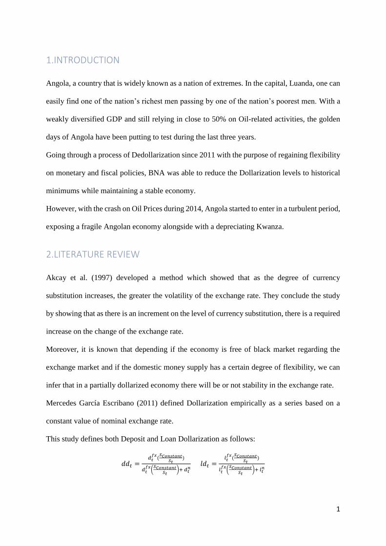
1.INTRODUCTION
Angola, a country that is widely known as a nation of extremes. In the capital, Luanda, one can
easily find one of the nation’s richest men passing by one of the nation’s poorest men. With a
weakly diversified GDP and still relying in close to 50% on Oil-related activities, the golden
days of Angola have been putting to test during the last three years.
Going through a process of Dedollarization since 2011 with the purpose of regaining flexibility
on monetary and fiscal policies, BNA was able to reduce the Dollarization levels to historical
minimums while maintaining a stable economy.
However, with the crash on Oil Prices during 2014, Angola started to enter in a turbulent period,
exposing a fragile Angolan economy alongside with a depreciating Kwanza.
2.LITERATURE REVIEW
Akcay et al. (1997) developed a method which showed that as the degree of currency
substitution increases, the greater the volatility of the exchange rate. They conclude the study
by showing that as there is an increment on the level of currency substitution, there is a required
increase on the change of the exchange rate.
Moreover, it is known that depending if the economy is free of black market regarding the
exchange market and if the domestic money supply has a certain degree of flexibility, we can
infer that in a partially dollarized economy there will be or not stability in the exchange rate.
Mercedes García Escribano (2011) defined Dollarization empirically as a series based on a
constant value of nominal exchange rate.
This study defines both Deposit and Loan Dollarization as follows:
𝑑𝑑𝑡 =𝑑𝑡
𝑓𝑥(
𝑆𝐶𝑜𝑛𝑠𝑡𝑎𝑛𝑡𝑆𝑡
)
𝑑𝑡𝑓𝑥
(𝑆𝐶𝑜𝑛𝑠𝑡𝑎𝑛𝑡
𝑆𝑡)+ 𝑑𝑡
𝑛 𝑙𝑑𝑡 =
𝑙𝑡𝑓𝑥
(𝑆𝐶𝑜𝑛𝑠𝑡𝑎𝑛𝑡
𝑆𝑡)
𝑙𝑡𝑓𝑥
(𝑆𝐶𝑜𝑛𝑠𝑡𝑎𝑛𝑡
𝑆𝑡)+ 𝑙𝑡
𝑛
2
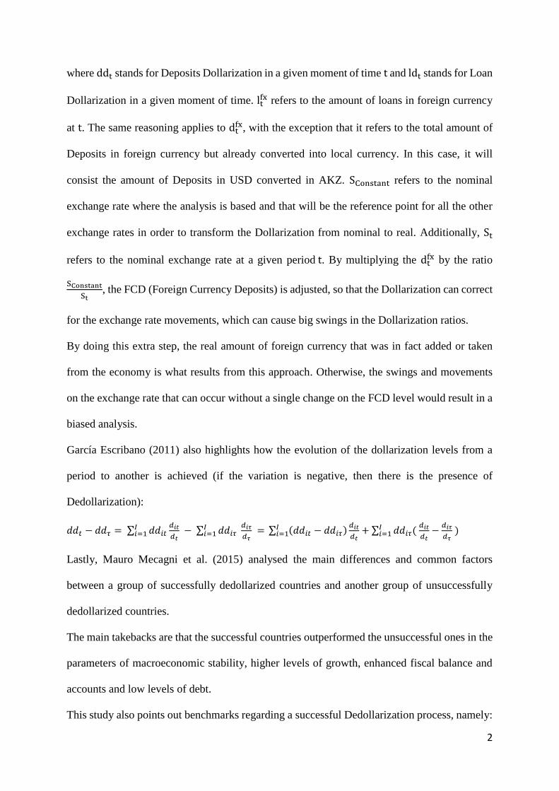
where ddt stands for Deposits Dollarization in a given moment of time t and ldt stands for Loan
Dollarization in a given moment of time. ltfx refers to the amount of loans in foreign currency
at t. The same reasoning applies to dtfx, with the exception that it refers to the total amount of
Deposits in foreign currency but already converted into local currency. In this case, it will
consist the amount of Deposits in USD converted in AKZ. SConstant refers to the nominal
exchange rate where the analysis is based and that will be the reference point for all the other
exchange rates in order to transform the Dollarization from nominal to real. Additionally, St
refers to the nominal exchange rate at a given period t. By multiplying the dtfx by the ratio
SConstant
St, the FCD (Foreign Currency Deposits) is adjusted, so that the Dollarization can correct
for the exchange rate movements, which can cause big swings in the Dollarization ratios.
By doing this extra step, the real amount of foreign currency that was in fact added or taken
from the economy is what results from this approach. Otherwise, the swings and movements
on the exchange rate that can occur without a single change on the FCD level would result in a
biased analysis.
García Escribano (2011) also highlights how the evolution of the dollarization levels from a
period to another is achieved (if the variation is negative, then there is the presence of
Dedollarization):
𝑑𝑑𝑡 − 𝑑𝑑𝜏 = ∑ 𝑑𝑑𝑖𝑡𝑑𝑖𝑡
𝑑𝑡 − ∑ 𝑑𝑑𝑖𝜏
𝑑𝑖𝜏
𝑑𝜏 =𝐼
𝑖=1 ∑ (𝑑𝑑𝑖𝑡 − 𝑑𝑑𝑖𝜏)𝑑𝑖𝑡
𝑑𝑡+ ∑ 𝑑𝑑𝑖𝜏(
𝑑𝑖𝑡
𝑑𝑡−
𝑑𝑖𝜏
𝑑𝜏 )𝐼
𝑖=1𝐼𝑖=1
𝐼𝑖=1
Lastly, Mauro Mecagni et al. (2015) analysed the main differences and common factors
between a group of successfully dedollarized countries and another group of unsuccessfully
dedollarized countries.
The main takebacks are that the successful countries outperformed the unsuccessful ones in the
parameters of macroeconomic stability, higher levels of growth, enhanced fiscal balance and
accounts and low levels of debt.
This study also points out benchmarks regarding a successful Dedollarization process, namely:
3
an overall reduction of 14% on the inflation level, unchanged exchange rates and a reduction
on public and external debt levels.
3.DOLLARIZATION
The process of Dollarization occurs when the local currency is substituted by a foreign
currency, usually US Dollar, and adopts the forms of store of value, unit of account and means
of payment.
It consists in a measure that most under-developed countries apply when they are facing
hyperinflation levels and a domestic currency depreciation, translating in economic instability.
Countries where there is a high level of inflation, which creates a real exchange rate instability,
tend to motivate residents to turn themselves to the foreign currency as it ensures a steadier
purchasing power regarding domestic consumption.
Dollarization ends up being perceived as a natural result of the progressive openness of the
emerging countries’ economies to the global economy. Starting in the 80’s, several emerging
economies went through Dollarization processes in the back of new exogenous shocks resulting
from a bigger level of exposure of the economy. There are several examples where the process
of Dollarization has been applied, especially in the emerging economies, namely: Russia in
1998, Peru in mid-70s and in 1990, among several others.
3.2 ADVANTAGES AND DISADVANTAGES OF DOLLARIZATION
There are several advantages on dollarizing an economy: asset substitution when a government
opens the economy and liberalizes the financial market, enhancement of the integration within
the international markets and most of the times it has an important role in the development of
domestic financial markets. Moreover, Dollarization mitigates the exchange rate risk for
foreign investors, attracting more investments for the country and allowing for a diversification
effect on the residents’ portfolio. Lastly, it has a positive impact in Investment and domestic
4
consumption and thus in economic growth, through a reduction on the cost of credit.
Nevertheless, Dollarization also carries several disadvantages, like the limitation of a country’s
monetary policy efficiency. It also implies that the country loses its seigniorage and has to pay
it to the foreign currency issuer. Moreover, the country’s efficiency on the daily transactions
and payments can be lost, since the central bank can no longer adapt their banknotes to the
population’s needs. Other aspect to take into account is the fact that dollarized economies are
highly exposed to the risk of occurring both a financial and currency crisis because of the lack
of power and control over their monetary policy. Lastly, by dollarizing an economy, the
liquidity risk will grow, meaning that small lenders only have access to unlimited funding in
domestic currency, so, in the case of general panic and bank runs, BNA cannot supply
unlimitedly the population with foreign currency, which can trigger a currency crisis.
Concluding, one can see that there is always a different and optimal level of dollarization to be
applied to a country, specially based on the economy’s size, openness, the degree of financial
integration and market development.
3.3 ANGOLA’S SITUATION WHEN DOLLARIZATION WAS INTRODUCED
By late 1990’s, Angola was in a very difficult and unstable economic period. The country was
suffering a sharp devaluation on their currency: Kwanza (AKZ) and the inflation was very high.
This bad economic shape was in part due to the civil war that was taking place at this period.
Since the purchasing power was dropping excessively in the eyes of the Angolan people, the
role of USD started to grow exponentially and got strong as the Government started to induce
the population to start using USD in order to stabilize the economy, i.e, inflation levels.
Therefore, in 2001, the Government decided to start the process of Dollarization of the economy
by applying several measures in order to counter attack the 241% inflation level that was being
seen at the time. As a result of this introduction, the real GDP growth took off in 2003 when it
started at a 3.5% and quickly evolving for an 11% in 2004.
5
In the case of Angola, the economy became partially dollarized, which implies a De facto
Dollarization, as an individual could easily use AKZ or USD to make a domestic payment or
transaction simultaneously. Additionally, by the fact that the overall banking system substituted
their structures to USD, it was in fact, a Financial Dollarization. Moreover, the foreign currency,
i.e. the USD, was used in domestic transactions, showing a characteristic of Transaction
Dollarization.
4.DEDOLLARIZATION
As already stated in the Literature Review, macroeconomic stabilization and stable and low
inflation are key ingredients for a successful dedollarization.
4.1 ANGOLA’S SITUATION WHEN DEDOLLARIZATION WAS APPLIED
During 2009, the majority of African countries were affected by the 2008 international crisis.
Due to its GDP exposure to Oil prices, Angola suffered a bigger hit, but also was able to rebound
quicker than the average, mainly because of the quick jump on Oil prices during the mid of
2009. Angola continued to recover during the year of 2010 especially after the signature of
Stand-by deals with the IMF, which gave a boost to the process of stabilizing the economy,
namely the rebalancing of the Government accounts. The latter was a major happening for
Angola to achieve a degree of credibility amongst the rest of the Sub-Saharan African
economies. Furthermore, for this economic recovery, factors like the rebalancing of the
Government budget in the Non-Oil Sectors and the initiative of public and private debt
regularization, played a major role.
Ultimately, in 2010 Angola was an economy that had re-gained the confidence of economic
agents, registering an astonishing increase in foreign investments.
Nevertheless, a Dollarization process also carries drawbacks and they were determinant in the
BNA decision of pursuing a De-dollarization process. Some of the the disadvantages appointed
6
by BNA’s analysis were the drop on Government’s liquidity because of the high share of
Foreign currency assets and liabilities compared to the national currency levels; the inefficiency
with payments in local currency; and the loss of control on the monetary policy of the Angolan
central bank. Adding the drawbacks of Dollarization that BNA was starting to realize to the
economy stability in terms of inflation and GDP growth, the decision of dedollarizing the
Angolan economy was voted and put into practice.
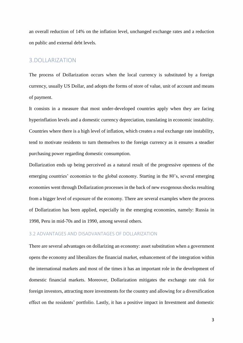
4.2 BNA’S MEASURES REGARDING DEDOLLARIZATION
Figure 1 Source: BNA
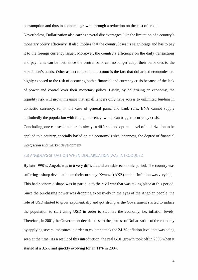
Figure 2 Source: BNA
After the decision of Dedollarizing the Angolan economy, BNA started to implement several
prudential measures. The willingness of the Angolan Central Bank to better the scenarios for
the national currency usage started from early 2010, period when BNA started to manage
7
closely the required level of reservoirs regarding the deposits. This influence was expected to
reduce the financing costs of the economic agents in order to incentivize the use of Kwanzas.
In terms of regulations sent out by BNA with the intention to promote a De-dollarizing process
in the Angolan economy, there are five promulgations that are worth to mention.
Chronologically, Aviso 5/2010 de 5 de Novembro – Exposição cambial was the first sizable
regulation introduced in the Angolan banking system. This law limited the liquid cambial
exposure (foreign currency assets minus foreign currency liabilities) to 20% of a regulated
financial institution’s ROF (Regulated Own Funds).
Secondly, Aviso 4/2011 de 8 de Junho – Crédito em moeda estrangeira, regulated the
concession and classification of loans given by BNA-regulated financial institutions.
They implemented a risk-grading system from A to G, starting in the riskless (A) and finishing
in the loss level (G) and forbidden the following credit operations in foreign currency.
Lastly, given the size and impact of Oil related investments and activities in Angola’s GDP, it
became obvious the need to differentiate the cambial legislation concerning the Oil sector from
the other economic activities. In this context, BNA published the Aviso 20/2012 de 25 de Abril
– Regime Cambial Sector Petrolífero, the biggest step taken towards the Dedollarization
process. It was designed to regulate the liquidation of equity and goods operations, and the cash
flows resulting from R&D, development and production of crude oil and natural gas.
5.THE BANKING SECTOR IN ANGOLA
This research project is based in the Banking sector especially because it is a perfect benchmark
for the country’s economic situation and performance. Angola has always had a significant
Financial Services Sector, however it intensified largely in the early 2000s, with a market
consolidation that today contemplates more than 30 Banking Institutions. Regarding the
analysis of the Banking Sector, it consists in three main components: the profitability, solvency
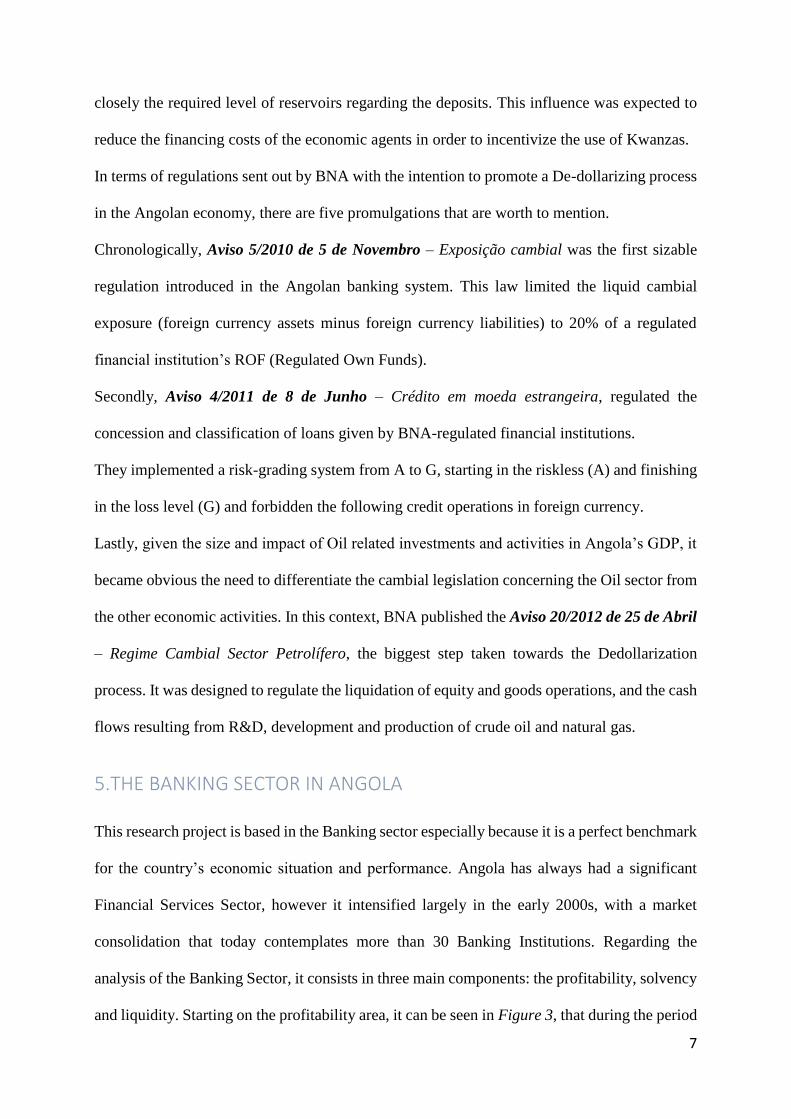
and liquidity. Starting on the profitability area, it can be seen in Figure 3, that during the period
8
after 2010 until 2014, almost all the major banks represented in the graphic suffered a drop on
their profitability.
Figure 3 Source: BNA and Bank’s Annual Reports Figure 4 Source: BNA
It was precisely during this period that the Dedollarization regulations started to show and
applied, showing à priori some sort of causality. Additionally, Figure 4 shows the average ROE
of all the Angolan Banking sector and how it has decreased throughout the period 2011-2015.
It can be also noted that from the last year and half, the sector has been regaining confidence
and strength. Nevertheless, a worrying aspect is the fact that the % of Non Performing Loans
is presenting an upward trend, a risk that represents nowadays represents 15% of loss on Banks’
returns coming from Loans.
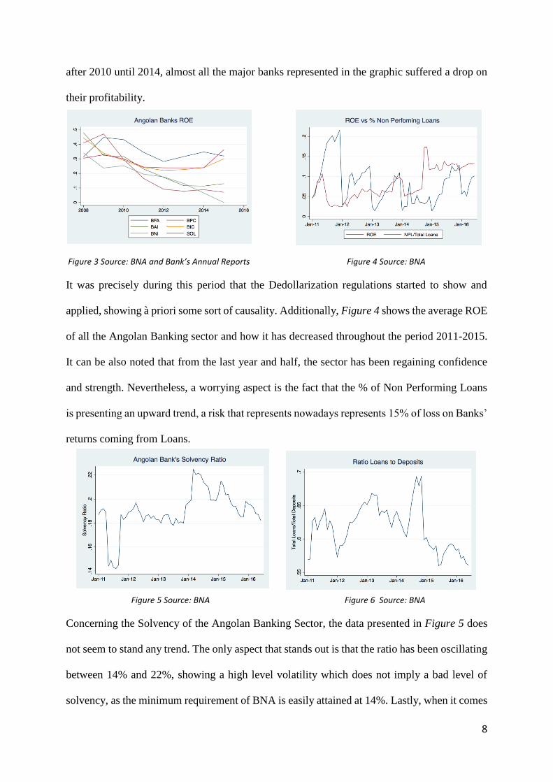
Figure 5 Source: BNA Figure 6 Source: BNA
Concerning the Solvency of the Angolan Banking Sector, the data presented in Figure 5 does
not seem to stand any trend. The only aspect that stands out is that the ratio has been oscillating
between 14% and 22%, showing a high level volatility which does not imply a bad level of
solvency, as the minimum requirement of BNA is easily attained at 14%. Lastly, when it comes
9
to the Liquidity, Figure 6 is very enlightening in the sense that the Banking system is already
assimilating a trend of more liquidity (less Loans), especially when the Non-Performing Loans
is increasing, which translates in a loss in the medium term. This trend is mostly visible after
January 2013 until June 2016.
6.BANCO DE FOMENTO DE ANGOLA - BFA
The fact that Angola has a data collection problem was determinant in the approach chosen for
this project in two ways. On one hand, it meant that a study about the impact on all the major
Angolan Banks would be literally impossible due to the inconsistency and lack of data, even
on the annual reports. On the other hand, the choice of BFA was achieved as it was the
institution that had a better control and records of their figures. Furthermore, besides the data
implications, BFA was a clear winner at the time of choosing an institution as it is one of the
most recognized and respectable Banks in Angola.
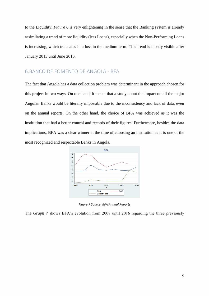
Figure 7 Source: BFA Annual Reports
The Graph 7 shows BFA’s evolution from 2008 until 2016 regarding the three previously
10
analysed components: Regulated Solvency Ratio, ROE and Liquidity Ratio. What immediately
stands out is the flat RSR, or at least, less volatile as the Banking sector average value. In fact,
if we take a look at Figure 8, we see how solid BFA is when compared to the Angolan average.
Figure 8 Source: BFA Annual Reports Figure 9 Source: BFA Annual Reports
The same applies when examining the ROE, with BFA attaining a spread of 20% compared
with the average of the Angolan Banking Sector. After the financial performance analysis is
done, it is required an overlook on the topic to which we are trying to evaluate the existence of
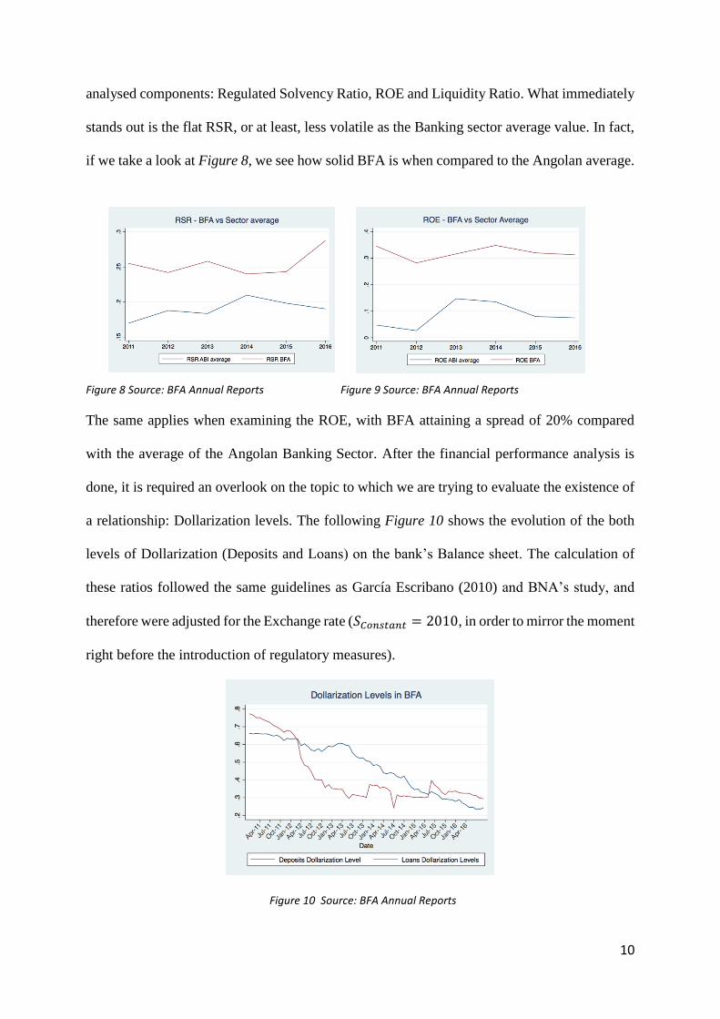
a relationship: Dollarization levels. The following Figure 10 shows the evolution of the both
levels of Dollarization (Deposits and Loans) on the bank’s Balance sheet. The calculation of
these ratios followed the same guidelines as García Escribano (2010) and BNA’s study, and
therefore were adjusted for the Exchange rate (𝑆𝐶𝑜𝑛𝑠𝑡𝑎𝑛𝑡 = 2010, in order to mirror the moment
right before the introduction of regulatory measures).
Figure 10 Source: BFA Annual Reports
11
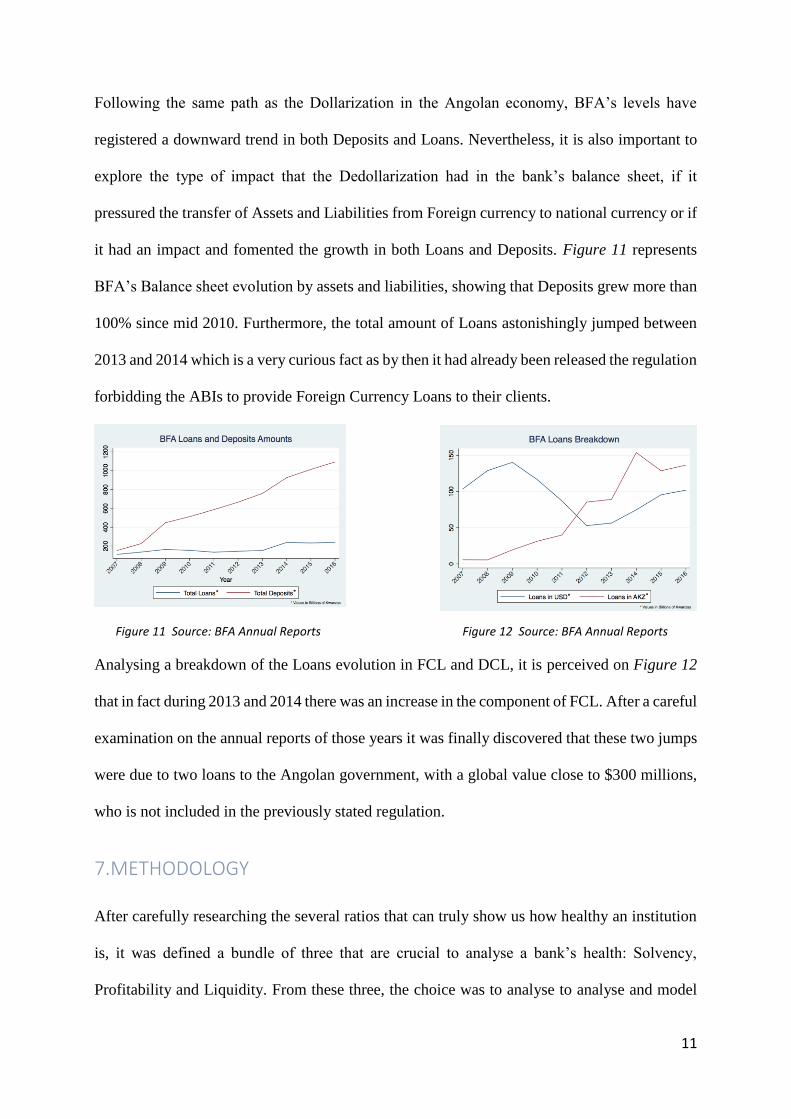
Following the same path as the Dollarization in the Angolan economy, BFA’s levels have
registered a downward trend in both Deposits and Loans. Nevertheless, it is also important to
explore the type of impact that the Dedollarization had in the bank’s balance sheet, if it
pressured the transfer of Assets and Liabilities from Foreign currency to national currency or if
it had an impact and fomented the growth in both Loans and Deposits. Figure 11 represents
BFA’s Balance sheet evolution by assets and liabilities, showing that Deposits grew more than
100% since mid 2010. Furthermore, the total amount of Loans astonishingly jumped between
2013 and 2014 which is a very curious fact as by then it had already been released the regulation
forbidding the ABIs to provide Foreign Currency Loans to their clients.
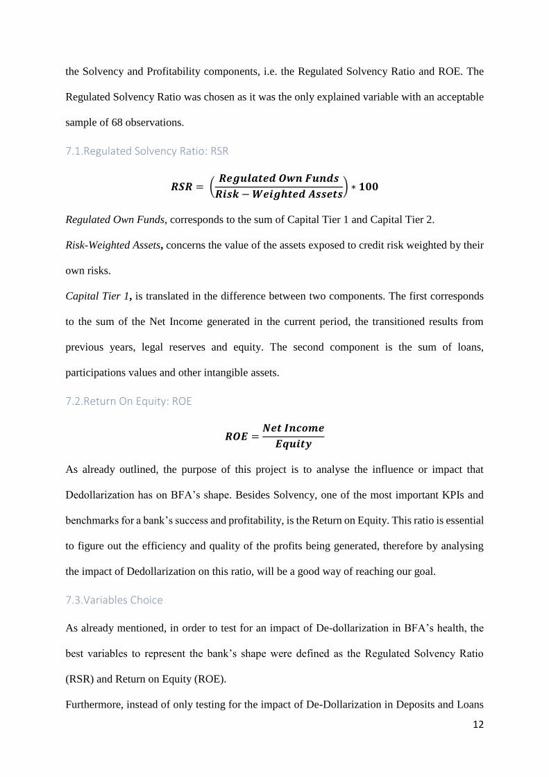
Figure 11 Source: BFA Annual Reports Figure 12 Source: BFA Annual Reports
Analysing a breakdown of the Loans evolution in FCL and DCL, it is perceived on Figure 12
that in fact during 2013 and 2014 there was an increase in the component of FCL. After a careful
examination on the annual reports of those years it was finally discovered that these two jumps
were due to two loans to the Angolan government, with a global value close to $300 millions,
who is not included in the previously stated regulation.
7.METHODOLOGY
After carefully researching the several ratios that can truly show us how healthy an institution
is, it was defined a bundle of three that are crucial to analyse a bank’s health: Solvency,
Profitability and Liquidity. From these three, the choice was to analyse to analyse and model
12
the Solvency and Profitability components, i.e. the Regulated Solvency Ratio and ROE. The
Regulated Solvency Ratio was chosen as it was the only explained variable with an acceptable
sample of 68 observations.
7.1.Regulated Solvency Ratio: RSR
𝑹𝑺𝑹 = (𝑹𝒆𝒈𝒖𝒍𝒂𝒕𝒆𝒅 𝑶𝒘𝒏 𝑭𝒖𝒏𝒅𝒔
𝑹𝒊𝒔𝒌 − 𝑾𝒆𝒊𝒈𝒉𝒕𝒆𝒅 𝑨𝒔𝒔𝒆𝒕𝒔) ∗ 𝟏𝟎𝟎
Regulated Own Funds, corresponds to the sum of Capital Tier 1 and Capital Tier 2.
Risk-Weighted Assets, concerns the value of the assets exposed to credit risk weighted by their
own risks.
Capital Tier 1, is translated in the difference between two components. The first corresponds
to the sum of the Net Income generated in the current period, the transitioned results from
previous years, legal reserves and equity. The second component is the sum of loans,
participations values and other intangible assets.
7.2.Return On Equity: ROE
𝑹𝑶𝑬 =𝑵𝒆𝒕 𝑰𝒏𝒄𝒐𝒎𝒆
𝑬𝒒𝒖𝒊𝒕𝒚
As already outlined, the purpose of this project is to analyse the influence or impact that
Dedollarization has on BFA’s shape. Besides Solvency, one of the most important KPIs and
benchmarks for a bank’s success and profitability, is the Return on Equity. This ratio is essential
to figure out the efficiency and quality of the profits being generated, therefore by analysing
the impact of Dedollarization on this ratio, will be a good way of reaching our goal.
7.3.Variables Choice
As already mentioned, in order to test for an impact of De-dollarization in BFA’s health, the
best variables to represent the bank’s shape were defined as the Regulated Solvency Ratio
(RSR) and Return on Equity (ROE).
Furthermore, instead of only testing for the impact of De-Dollarization in Deposits and Loans
13
in these BFA’s KPIs, this approach will also try to analyse exogenous variables to the bank, as
they are also being affected by the Dedollarization process at some extent.
Therefore, I divided the explanatory variables in three main groups: BFA-related variables,
macroeconomic variables and prudential measures variables. Concerning the BFA-related
variables, I chose BFA’s Loans (LD) and Deposits Dollarization (DD) Levels as two predictors
for the Dedollarization level. As we know, a decrease in the Dollarization ratio represents an
increase in the Dedollarization of the economy. When it comes to the Macroeconomic variables,
I opted to include five different variables so that they could mirror the Angolan’s economy
performance at a given period. Thus, I decided to use: Exchange Rate (EX), as it reflects the
appreciation (Dedollarization) or not of the Kwanza and impacts the Bank’s results and
solvability; Inflation (INF), in order to assess the direct relation that it has on the bank, as its
increase puts a pressure on BFA clients’ Kwanzas Deposits; Oil Prices (OIL), which was an
external event that brought a massive shock to the Angolan GDP, therefore having an impact
on the banking sector; Exchange Rate Spread (EX_SPREAD), so that I am able to see whether
the credibility and trust that the Angolans affects BFA; and finally, 3 month Angolan Treasury
Bills (BT) which will work as a benchmark of Angola’s risk evolution. Lastly, regarding the
prudential measures variables, instead of creating dummy variables in order to incorporate the
three main regulations that BNA launched towards a Dedollarization process, I decided to come
up with endogenous variables that work as proxies to the effects of these measures, namely:
Foreign Currency Loans Level (FCL), which refers to the Aviso 4/2011 de 8 de Junho, which
stated that financial institutions would no longer be able to concede loans in USD to their
clients; and Domestic Currency Deposits Level (DCL), which is related to Aviso 20/2012 de 25
de Abril, the major regulation directed to the Oil sector. The latter variable helps to reflect the
impact in the sense that this regulation made Oil companies to not only open Kwanzas accounts,
but it also made them to transfer funds from their USD accounts to Kwanzas accounts.
14
The approach taken for building both models was the same and based in four main steps:
1) Create a correlation matrix between every variable with the main purpose to identify
the ones with a low absolute correlation factor to the dependent variables and cut some
of the variables that do not contribute for the problem being studied.
2) Before starting the model, it is necessary to test for stationarity in all the variables as
they are time-series, using the Augmented Dickey Fuller Unit Root test and correct them
for stationarity, so that a biased conclusion on the model’s significance is avoided.
3) Construct a multi-factor regression model and obtain the one that maximizes the
Adjusted 𝑅2. For this stage, a stepwise backwards approach was undertaken, starting by
the full model and decreasing at each time the number of insignificant variables until an
optimal level was reached.
4) Finally, take conclusions on the statistical meaning of the findings based on the
significance levels of each of the variables and their economic meaning.
7.4.RSR Multi-factor Regression
For this model, the sample considered ranged from September 2011 until September 2016 on a
monthly basis, meaning an N= 60 observations. This sample size is explained by the fact that
BFA only started to calculate its Regulated Solvency Ratio on a monthly basis in 2011 and that
the calculation of RSR took a major improvement in September 2011.
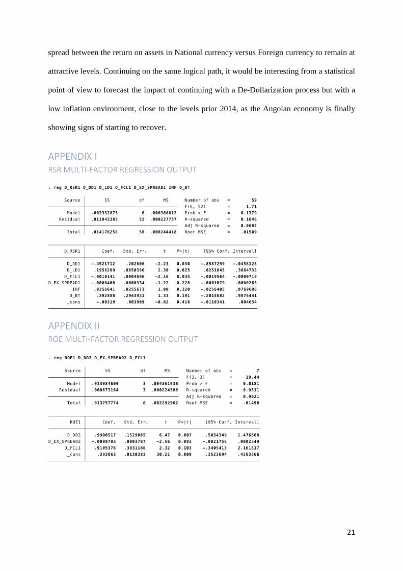
After proceeding with previously detailed approach, the final model obtained was the following
(see Appendix I for the regression output):
𝐷_𝑅𝑆𝑅𝑡−1 = 𝛼 + 𝛽1. 𝐷𝐷𝐷𝑡−1 + 𝛽2. 𝐷𝐿𝐷𝑡−1 + 𝛽3. 𝐷𝐹𝐶𝐿𝑡−1+ 𝛽4. 𝐷_𝐸𝑋_𝑆𝑃𝑅𝐸𝐴𝐷𝑡−1 + 𝛽5. 𝐼𝑁𝐹𝑡 + 𝛽6 . 𝐷_𝐵𝑇𝑡 + 𝜇𝑡
𝐷_𝑅𝑆𝑅𝑡−1 : First Difference of Variable RSR with Lag 1.
𝐷_𝐷𝐷𝑡−1 : First Difference of Variable DD with Lag 1.
𝐷_𝐹𝐶𝐿𝑡−1 : First Difference of Variable FCL with Lag 1.
𝐷_𝐸𝑋_𝑆𝑃𝑅𝐸𝐴𝐷𝑡−1 : First Difference of Variable D_EX_SPREAD with Lag 1.
𝐼𝑁𝐹𝑡: Variable INF
𝐷_𝐵𝑇𝑡: First Difference of Variable BT
15
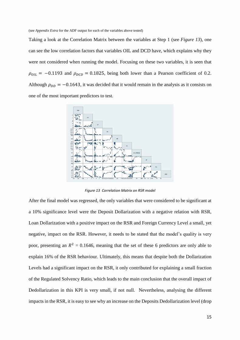
(see Appendix Extra for the ADF output for each of the variables above tested)
Taking a look at the Correlation Matrix between the variables at Step 1 (see Figure 13), one
can see the low correlation factors that variables OIL and DCD have, which explains why they
were not considered when running the model. Focusing on these two variables, it is seen that
𝜌𝑂𝐼𝐿 = −0.1193 and 𝜌𝐷𝐶𝐷 = 0.1825, being both lower than a Pearson coefficient of 0.2.
Although 𝜌𝐷𝐷 = −0.1643, it was decided that it would remain in the analysis as it consists on
one of the most important predictors to test.
Figure 13 Correlation Matrix on RSR model
After the final model was regressed, the only variables that were considered to be significant at
a 10% significance level were the Deposit Dollarization with a negative relation with RSR,
Loan Dollarization with a positive impact on the RSR and Foreign Currency Level a small, yet
negative, impact on the RSR. However, it needs to be stated that the model’s quality is very
poor, presenting an 𝑅2 = 0.1646, meaning that the set of these 6 predictors are only able to
explain 16% of the RSR behaviour. Ultimately, this means that despite both the Dollarization
Levels had a significant impact on the RSR, it only contributed for explaining a small fraction
of the Regulated Solvency Ratio, which leads to the main conclusion that the overall impact of
Dedollarization in this KPI is very small, if not null. Nevertheless, analysing the different
impacts in the RSR, it is easy to see why an increase on the Deposits Dedollarization level (drop
16
on the Deposits Dollarization Level) would lead to an increment in the Regulated Solvency
Ratio: given that the bank’s solvency is seen as its ability to repay its debt obligations in the
medium-long term, a decrease in the USD obligations (USD deposits) is a positive event for
the bank, as it becomes more solid. This is explained by the fact that at the current state of the
Angolan economy, BNA struggles a lot to provide USD to the economy, so if a bank’s
obligations sheet is in Kwanzas, it will be a lot easier for BNA to support it.
7.5.ROE Multi-factor Regression
For this model, the sample considered ranged from 2007 until 2016 on a yearly basis, meaning
a N= 9 observations. Though the size of sample was remarkably low, an attempt to stablish a
relation between BFA’s Return on Equity and the change in the Dollarization levels was
undertaken. The main reason for such initiative relies on the fact the component of profits and
equity structure captured by ROE is the most important for the analysis of the bank’s situation.
After proceeding with the previously detailed approach, the final model obtained was the
following (see Appendix II for the regression output):
𝑅𝑂𝐸𝑡−1 = 𝛼 + 𝛽1 . 𝐷_𝐷𝐷𝑡−2 + 𝛽2. 𝐷_𝐸𝑋_𝑆𝑃𝑅𝐸𝐴𝐷𝑡−2 + 𝛽3. 𝐷_𝐹𝐶𝐿𝑡−1 + 𝜇𝑡
𝑅𝑂𝐸𝑡−1 : Variable ROE with Lag 1.
𝐷_𝐷𝐷𝑡−2 : First Difference of Variable DD with Lag 2.
𝐷_𝐸𝑋_𝑆𝑃𝑅𝐸𝐴𝐷𝑡−2 : First Difference of Variable D_EX_SPREAD with Lag 1.
𝐷_𝐹𝐶𝐿𝑡−1 : First Difference of Variable FCL with Lag 1.
(see Appendix Extra for the ADF output for each of the variables above tested)
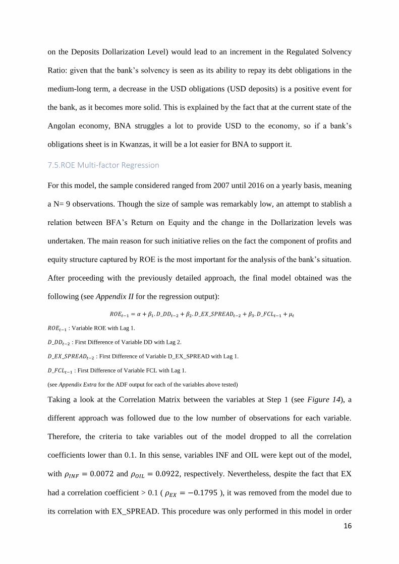
Taking a look at the Correlation Matrix between the variables at Step 1 (see Figure 14), a
different approach was followed due to the low number of observations for each variable.
Therefore, the criteria to take variables out of the model dropped to all the correlation
coefficients lower than 0.1. In this sense, variables INF and OIL were kept out of the model,
with 𝜌𝐼𝑁𝐹 = 0.0072 and 𝜌𝑂𝐼𝐿 = 0.0922, respectively. Nevertheless, despite the fact that EX
had a correlation coefficient > 0.1 ( 𝜌𝐸𝑋 = −0.1795 ), it was removed from the model due to
its correlation with EX_SPREAD. This procedure was only performed in this model in order
17
to ensure the maximum quality and significance possible given the sample size constraint.
Figure 14 Correlation Matrix on ROE model
After the final model was regressed, only Deposits Dollarization and the Exchange Rate Spread
were considered to be significant at a 10% significance level. Contrary to the previous model,
this model presented a 𝑅2= 0.9511, a clear sign of significance and relevance of the two
predictors. Taking into account the problem of sample size, this result only means that there
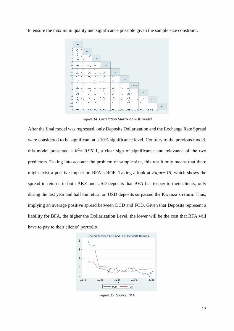
might exist a positive impact on BFA’s ROE. Taking a look at Figure 15, which shows the
spread in returns in both AKZ and USD deposits that BFA has to pay to their clients, only
during the last year and half the return on USD deposits surpassed the Kwanza’s return. Thus,
implying an average positive spread between DCD and FCD. Given that Deposits represent a
liability for BFA, the higher the Dollarization Level, the lower will be the cost that BFA will
have to pay to their clients’ portfolio.
Figure 15 Source: BFA
18
8.MAIN CONCLUSIONS
As previously explained, a Dedollarization process is undertaken in order to restore monetary
and fiscal policy autonomy. Usually, it means that the foreign currency is swapped by the local
currency and re-gains use in most of its forms: store of value, means of payment and unit of
account. Nevertheless, in the case of Angola there has been a successful transition from USD
to Kwanzas in the forms of means of payment and unit of account. By recalling Figures 1 and
2, it is easily seen how the impact of BNA’s prudential measures had a statement in bringing
down the Dollarization Levels in both Deposits and Loans to levels close to 20% in only 5
years. As Departamento de Estudos Económicos (2014) state in their article, until 2013 Angola
was being very successful on Dedollarizing its economy, mainly due to the role of BNA, which,
back in 2013, was able to achieve a stable macroeconomic environment and a working stimulus
to take the USD out of the economy. Ultimately, the department was able to prove in their
study, that Dedollarization and macroeconomic stability share an interdependent relation.
However, fast-forwarding to 2016, it is seen that the process was not fully completed: inflation
levels close to 40%, a never-ending Kwanza devaluation and yet, the banking system presents
a balance-sheet with low levels of USD Assets and Liabilities. Additionally, the shock on oil
prices brought high levels of inflation and an abrupt devaluation of Kwanza which made people
to pursuit the USD, as it is known that on a recent dollarized economy, whenever there is an
external shock, people tend to protect themselves with foreign currency. This event was critical
in making the population of Angola very cautious regarding Kwanza as a form of store of value.
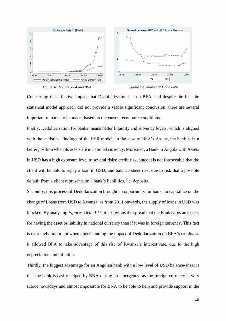
Taking a look at Figure 16, the increasing values for Kwanza that are being exchanged in the
Parallel Market are pushing the exchange rate to astonishing levels, showing the low level of
credibility that Kwanza has close to the population. Moreover, this trend can be also seen by
the fact that most of the Angolans are buying USD indexed Treasury Bill at a very large growth
rate, to protect from a depreciating Kwanza.
19
Figure 16 Source: BFA and BNA Figure 17 Source: BFA and BNA
Concerning the effective impact that Dedollarization has on BFA, and despite the fact the
statistical model approach did not provide a viable significant conclusion, there are several
important remarks to be made, based on the current economic conditions.
Firstly, Dedollarization for banks means better liquidity and solvency levels, which is aligned
with the statistical findings of the RSR model. In the case of BFA’s Assets, the bank is in a
better position when its assets are in national currency. Moreover, a Bank in Angola with Assets
in USD has a high exposure level to several risks: credit risk, since it is not foreseeable that the
client will be able to repay a loan in USD; and balance sheet risk, due to risk that a possible
default from a client represents on a bank’s liabilities, i.e. deposits.
Secondly, this process of Dedollarization brought an opportunity for banks to capitalize on the
change of Loans from USD to Kwanza, as from 2011 onwards, the supply of loans in USD was
blocked. By analysing Figures 16 and 17, it is obvious the spread that the Bank earns an excess
for having the asset or liability in national currency than if it was in foreign currency. This fact
is extremely important when understanding the impact of Dedollarization on BFA’s results, as
it allowed BFA to take advantage of this rise of Kwanza’s interest rate, due to the high
depreciation and inflation.
Thirdly, the biggest advantage for an Angolan bank with a low level of USD balance-sheet is
that the bank is easily helped by BNA during an emergency, as the foreign currency is very
scarce nowadays and almost impossible for BNA to be able to help and provide support in the
20
case of an unexpected event.
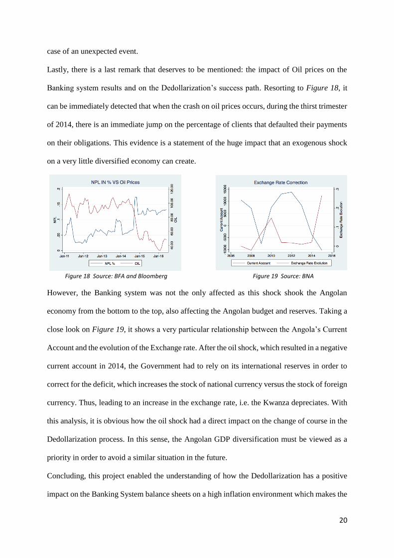
Lastly, there is a last remark that deserves to be mentioned: the impact of Oil prices on the
Banking system results and on the Dedollarization’s success path. Resorting to Figure 18, it
can be immediately detected that when the crash on oil prices occurs, during the thirst trimester
of 2014, there is an immediate jump on the percentage of clients that defaulted their payments
on their obligations. This evidence is a statement of the huge impact that an exogenous shock
on a very little diversified economy can create.
Figure 18 Source: BFA and Bloomberg Figure 19 Source: BNA
However, the Banking system was not the only affected as this shock shook the Angolan
economy from the bottom to the top, also affecting the Angolan budget and reserves. Taking a
close look on Figure 19, it shows a very particular relationship between the Angola’s Current
Account and the evolution of the Exchange rate. After the oil shock, which resulted in a negative
current account in 2014, the Government had to rely on its international reserves in order to
correct for the deficit, which increases the stock of national currency versus the stock of foreign
currency. Thus, leading to an increase in the exchange rate, i.e. the Kwanza depreciates. With
this analysis, it is obvious how the oil shock had a direct impact on the change of course in the
Dedollarization process. In this sense, the Angolan GDP diversification must be viewed as a
priority in order to avoid a similar situation in the future.
Concluding, this project enabled the understanding of how the Dedollarization has a positive
impact on the Banking System balance sheets on a high inflation environment which makes the
21
spread between the return on assets in National currency versus Foreign currency to remain at
attractive levels. Continuing on the same logical path, it would be interesting from a statistical
point of view to forecast the impact of continuing with a De-Dollarization process but with a
low inflation environment, close to the levels prior 2014, as the Angolan economy is finally
showing signs of starting to recover.
APPENDIX I
RSR MULTI-FACTOR REGRESSION OUTPUT
APPENDIX II ROE MULTI-FACTOR REGRESSION OUTPUT
22
REFERENCES
Kokenyne, Annamaria and Ley, Jeremy and Veyrune, Romain. 2010, “Dedollarization.”,
IMF Working Paper 10/188.
García Escribano, Mercedes. 2010. “Peru: Drivers of De-dollarization.”, IMF Working
Paper 10/169.
Mengesha, Lula G. and Holmes, Mark J.. 2013. “Does Dollarization Alleviate or
Aggravate Exchange Rate Volatility?.”, Journal of Economic Development, 38(2).
Ponomarenko, Alexey and Solovyeva, Alexandra and Vasilieva, Elena. 2011. “Financial
dollarization in Russia: causes and consequences.”, BOFIT Discussion Papers, 36.
Mecagni, Mauro and Maino, Rodolfo. 2015. “Dollarization in Sub-Saharan Africa.”, IMF
African Department.
Ize, Alain and Yeyati, Eduardo L.. 2003. “Financial dollarization.”, Journal of
International Economics, 59: 323-347.
De Nicoló, Gianni and Honohan, Patrick. and Ize, Alain. 2004. “Dollarization of bank
deposits: Causes and consequences.”, Journal of Banking & Finance, 29: 1697-1727.
Kokenyne, Annamaria and Ley, Jeremy and Veyrune, Romain. 2010, “Dedollarization.”,
IMF Working Paper 10/188.
Mwase, Nkunde and Kumah, Francis Y.. 2015. “Revisiting the Concept of Dollarization:
The Global Financial Crisis and Dollarization in Low-Income Countries”, IMF Working
Paper 15/12.
García-Escribano, Mercedes and Sosa, Sebastián. 2011, “What is Driving Financial De-
dollarization in Latin America?”, IMF Working Paper 11/10.