The Pennsylvania State University College of Earth and Mineral Sciences

Department of Geosciences

Examining the Age Distribution of Peromyscus Remains in Parker’s Pit Cave, Custer County, SD

A Senior Thesis in Geobiology

by

Joel A. Christine

Submitted in Partial Fulfillment of the Requirements

for the Degree of

Bachelor of Science

December, 2008

We approve this thesis: ________________________________________ _______________ Russell Graham, Professor of Geosciences Date Director, EMS Museum ________________________________________ _______________ David M. Bice, Professor of Geosciences Date Associate Head of the Undergraduate Program

1

Age Distribution of Peromyscus in Parker’s Pit Cave Joel A. Christine

ABSTRACT

Caves are an interesting and useful source of fossil material from the Pleistocene

and Holocene Epochs. An example of this is Parker’s Pit Cave, in the Black Hills region

of South Dakota, which has been excavated over the course of multiple summers by a

Penn State University team. Among a variety of small animal bones that were recovered

from this cave are those of the rodent Peromyscus, commonly known as the deer mouse.

Those bones were found at two separate locations within Parker’s Pit – a former entrance

called Red Cone and the current entrance, Main Cone. A study of age distribution for the

mice at these sites, determined from the wear on their molars, shows a statistically

significant difference between the two entrances. This is indicative of different bone

accumulation processes at each site, and thus of different taphonomic biases. Main Cone

exhibits a basically random collection of deer mice over a wide range of ages, reflecting

its nature as an unselective pitfall trap. Red Cone consists almost solely of younger mice,

consistent with demonstrated preferences of predators that feed upon rodents. Additional

study has shown that Main and Red Cones also differ significantly in age distribution

from an averaged wild population of Peromyscus. Microscopic study of two Peromyscus

jaw samples from the different debris cones showed differences in their external physical

condition. The Main Cone jaw appears to be in fairly good condition, whereas the Red

Cone jaw shows evidence of breakage, chemical surface erosion and discoloration. These

findings are also consistent with the proposed differences in how the bones accumulated

at each site, and thus merit further study.

2

INTRODUCTION

For most people the traditional vision of paleontology is one of digging into the

hot, sun-baked sands of a remote desert for fossils. But as it turns out, caves are another

viable source for evidence of past life. Some paleontologists actually specialize in cave-

based studies of ancient animals. Interestingly, caves are not permanent features but have

a “life cycle” of sorts that occurs over millions of years. A cave opens in the ground,

expands and extends over a period ranging from thousands to millions of years, and

eventually either collapses or fills up with sediment (Andrews, 1990; Brain, 1981). As a

result, most caves are geologically relatively recent products of natural processes, and the

paleontologists who hunt for fossils inside caves tend to study life in the Pleistocene

and/or Holocene epochs (Andrews, 1990; Brain, 1981; Graham, 2008). For several years

there has been an effort to excavate within two closely spaced caves in the Black Hills

National Forest, South Dakota, in order to study questions of North American

paleoecology and biogeography (Graham, 2008). But as with cave-based studies in

general, the scientists in this project need a thorough understanding of the preservational

biases at work in cave settings. In an effort to contribute to that understanding, I studied

the remains of deer mice (genus Peromyscus) found in one of these caves, known as

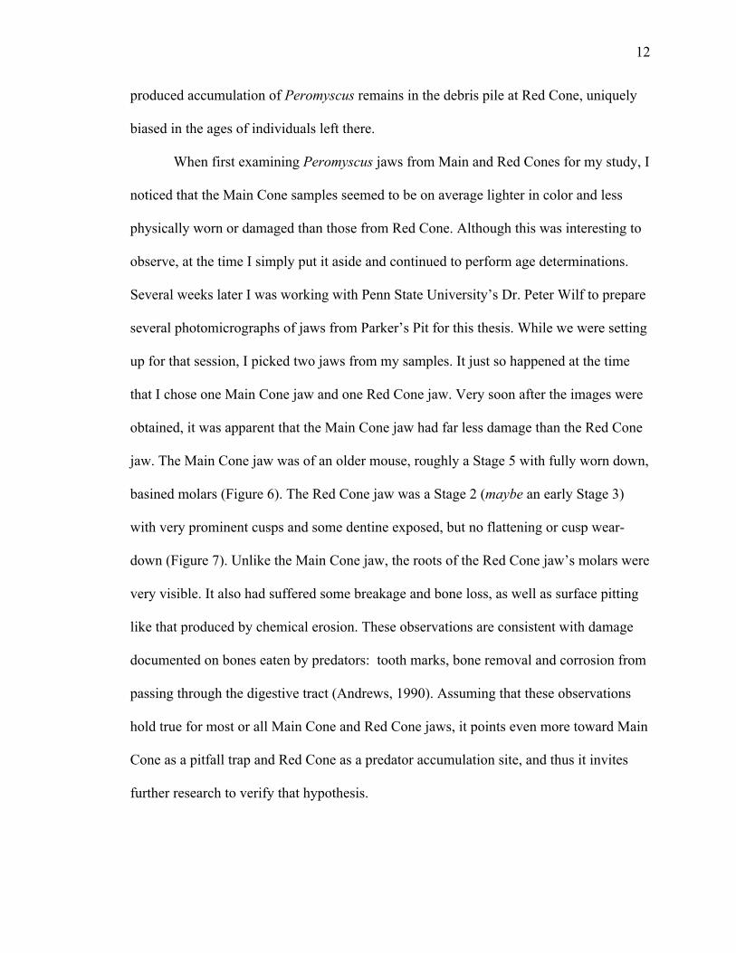
Parker’s Pit (Figure 1).

There are several ways in which animals can end up inside caves. Some may

actually live or hide in the cave; others can fall in and become trapped; predators may

bring their kills to a cave before consuming them; and bodies can be transported into a

cave post mortem (Andrews, 1990). Studies of cave fossils to determine just how they

arrived and what patterns (or biases) may have been introduced into that cave’s record

3

involve taphonomy – the formal study of fossilization processes (Andrews, 1990; Brain,

1981; Foote and Miller, 2007). An entrance that randomly traps animals should retain a

range of species that live in the general vicinity of the cave, in contrast to materials that

are carried into the cave by carnivores and/or raptors. Different kinds of predators will eat

different prey, leaving their own unique feeding signature – their selective bias – behind

(Andrews, 1990; Brain, 1981; Bryant, 1991; Graham, 2008). It has been shown that while

owls may hunt across a broad area (up to several square kilometers), they will leave

regurgitated pellets from their meals at their roosts in or near the cave entrance. So any

differences in food preferences will be reflected in the owl pellet contents (Andrews,

1990; Brain, 1981).

A predator’s success can depend upon the age – and thus the experience level – of

its target prey. This can also show up in the remains left behind (Bryant, 1991; Lyman et

al., 2001), and can be detected if one knows how to determine the age of the animal

remains (Lyman et al., 2001; Morris, 1972). Studying the age of animals within a

population or other group can also be informative in other ways. It can reveal knowledge

of population dynamics and ecology, and allow for the comparison of characteristics

between groups (Bryant, 1991).

As some ages of animals are more vulnerable to predation than others, age

determination of cave remains can help to distinguish between a pitfall trap and a

predator’s accumulation. For example, because of their size small animals may survive

falling into a pit cave. (A smaller animal reaches a lower relative “terminal velocity” due

to the proportionally higher resistance to air flow around its body.) The cave’s new

residents would likely be safe and sheltered from bad weather, as well. It has been shown

4

that in some cases animals trapped in a cave can survive for extended periods of time by

feeding on detritus that falls in (Andrews, 1990). The isolated environment of a pit cave

also lacks natural predators, which enhances an animal’s longevity. These factors could

allow animals that fall in at the Parker’s Pit main entrance and survive to remain alive for

a long time. With enough food falling into the cave, these animals could live to old age

despite being trapped. On the other hand, carnivores often select younger – and thus

inexperienced – individuals as prey. This choice makes capture and killing of food easier

and more productive than with older animals. Thus the age distribution of mice remains

found in a cave may provide information on their origin.

Most research in age determination involves live animals, and often uses soft tissue

to determine how old an individual is (Morris, 1972). But in many cases, including caves

and owl pellets, only the hard parts like bones and teeth are left to examine; they are often

separated after death and may be damaged by various processes (Andrews, 1990; Brain,

1981). For small mammals like rodents, the durability and distinctiveness of teeth make

them a useful and sometimes preferred choice for age determinations (Bryant, 1991;

Macêdo, et al., 1987; Morris, 1972; de Oliveira, et al., 1998; Sheppe, 1963).

As a mammal ages it feeds on its preferred range of foods, which eventually wears

down the enamel on its teeth. Studies have shown that tooth wear, specifically molar

wear in rodents, can serve as an effective proxy for relative age (Bryant, 1991; Lyman et

al., 2001; Morris, 1972; de Oliveira, et al., 1998; Sheppe, 1963). In my study of deer

mice from Parker’s Pit, there was an overwhelming abundance of lower jaws from

Peromyscus. Along with limited resources and time, this restricted the choices of age

determination techniques to examining tooth wear. Several weeks were spent researching

5

various, often similar, criteria for age determination of rodents based on dental wear. In

the end, a decision was made to modify the five-stage system devised by Walter Sheppe

(1963) specifically for studying Peromyscus in the Pacific Northwest of North America.

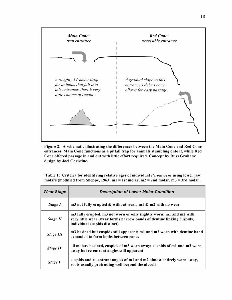
At Parker’s Pit there are two debris cones of interest: Main Cone and Red Cone

(Figure 1). Main Cone is located at the primary current entrance, which has a 12-meter

vertical drop. The current main entrance thus is a trap for animals that stumble into it. On

the other hand, Red Cone is a filled former entrance with an inclined debris cone; this

cone appears to have a shallow enough slope for easy entrance and egress. This would

have made Red Cone useful for predators as a site for feeding, but not an effective trap

(Figure 2). The respective accumulations of deer mice remains at each entrance’s debris

pile or cone should then reflect different pathways. My hypothesis is that the Peromyscus

populations at Main Cone and Red Cone are different in their age distributions: Red

Cone will have predominantly younger individuals because of its use as a predator

accumulation, whereas Main Cone will have older mice that were trapped but were likely

to have survived in a predator-free environment.

METHODS

The lower jaws of Peromyscus that were used in my research were obtained –

along with a variety of other fossil specimens – from Parker’s Pit over the course of

several summers. The original sediments were excavated from the two debris piles, one at

Main Cone and another at Red Cone, in increments of ten centimeters. As these

sediments were removed they were bagged, weighed and individually numbered, then set

aside for processing later. The first step in the processing of material was screen washing

6

using a 3-mm mesh to remove all soluble material and the very smallest of insoluble

particles. The bag numbers were recorded in a notebook as well as on the labeled bags of

residue from the screen washings (Graham, 2008).

Statistical standards require a minimum sample size of about 20-30 data points in

order to use the working assumption that the population under study has a normal

distribution of the characteristic(s) of interest. The purpose of this is to, at least in

principle, make the statistical analysis simpler and easier. With that in mind, I picked out

a total of 45 Peromyscus lower jaws from bags of material taken from Main Cone and

Red Cone (23 jaws from the former and 22 from the latter). The jaws were placed into

small paper cups as I picked them out, and at the end of each session I placed the jaws in

smaller “ziplock” style plastic bags for storage. For each jaw or set of jaws in a particular

bag from Parker’s Pit, I reproduced the field data from the original bag onto a small paper

tag for later reference. These tags were kept in the small ziplock bags to keep track of

where each jaw came from.

The system that I used to judge the relative age of a jaw was derived from one

published in 1963 by Walter Sheppe, who had studied live populations of deer mice in

both British Columbia, Canada and in the northwestern US state of Washington.

Sheppe’s system had five stages of wear ranging from Stage 1 for the youngest to Stage 5

for the oldest. His system, like other similar systems for rodent age determination, used

upper jaw molars. Since I had almost no upper jaws to use, my thesis adviser and I

modified Sheppe’s criteria to make it more applicable to my samples (Table 1). Using

these adjusted wear criteria, I examined each lower jaw with a binocular microscope for

molar wear to determine an age level for that individual. In many cases I had to gently

7

brush debris off of the jaws using a small paintbrush that I moistened with water before

use. Where the degree of tooth wear on a jaw appeared to be between two levels in our

criteria, I conservatively chose the lower applicable age level. The age levels were

recorded in a data sheet for later filling out of an Excel® spreadsheet; for each jaw

recorded I also put in the data on the Parker’s Pit field bag that it came from.

The next task was to plot a histogram of age classes for each cone’s population.

This allowed me to easily see any pattern in the age distributions, and compare that to

patterns of distribution found within a living population of Peromyscus. As it happens,

the report by Walter Sheppe that provided me with an age-determination system also had

data on the age structure of two wild deer mice populations. One was of Peromyscus

oreas, total population 274; the other of Peromyscus maniculatus, total population 376.

My samples were not identified as to species, so I combined and then averaged the data

for Sheppe’s wild populations. The averaged sample’s total size was 320.5, much larger

than the Parker’s Pit samples of 23 and 22. To make comparisons easier, I adjusted or

“normalized” the averaged Sheppe population down to a total closer in size to Main and

Red Cones: 21 individuals. I then plotted that set in a histogram as I had done with Main

and Red Cones. I now had three data sets for comparison (Table 2; Figures 3, 4, and 5).

For my statistical analysis I used the Student’s t-test, which compares separate

data sets to determine their degree of similarity. One decides upon a null hypothesis that

the two sets to be compared have no statistically significant differences, and so are

indistinguishable from samples taken out of a larger, normally distributed population.

The alternative hypothesis – what one hopes to demonstrate – is that the two sample sets

are in fact significantly different from each other and thus reflect two different

8

populations and/or two different processes. The result of the t-test is either rejection of

the null hypothesis or failure to reject it, along with a confidence level at which the result

is statistically significant. My null hypothesis in this study was that the two sample

populations – Main Cone and Red Cone – would show no significant differences in their

age distributions. My alternative hypothesis was that in comparing Main Cone with Red

Cone, there would be a statistically significant level of difference in their respective age

distributions, which would reflect a difference in either the populations that they came

from or the processes that accumulated Peromyscus at the two entrances. A similar set of

null and alternative hypotheses were devised for my comparisons between Main and Red

Cones on one hand and the Sheppe data on the other.

RESULTS

In tabulating the results for Main and Red Cone’s sample populations, there are

both similarities and differences that are easy to discern (Figures 3 & 4; Table 2). Both

cones have mainly Stage 3 individuals (13 for each site), no Stage 1 individuals, and

more Stage 2s than either Stage 4 or Stage 5. But Main Cone has only five Stage 2s,

balanced out by three Stage 4s and two Stage 5s. Red Cone on the other hand has eight

Stage 2s and a single Stage 4, with no Stage 5 individuals. Clearly the population at Red

Cone is younger overall than that at Main Cone.

The averaged wild Peromyscus population from Sheppe’s study shows yet

another variation in age distribution (Table 2). Like Main and Red Cones its deer mice

are a younger group as a whole, but here Stage 2 is the most abundant stage at 14 total.

Stages 3 and 4 have four and two respectively, while Stage 1 has a single representative

9

and no Stage 5s (this last result is due to a rounding issue in proportionally reducing the

sample size). So Sheppe’s deer mice populations were generally younger as a whole than

were those found in Parker’s Pit.

The Student’s t-test results showed that the two sample populations were more

different than alike in their age distribution patterns (Table 3). The comparison of Main

Cone to Red Cone demonstrated to a 95.5% confidence level that they were statistically

dissimilar to each other. This suggests that they represent either different populations or

the results of different processes. Likewise, in comparing Main Cone to Sheppe (99.8%

confidence level) and Red Cone to Sheppe (91.8% confidence level), the differences in

age distribution outweighed the similarities. This also suggests either difference source

populations or different processes.

DISCUSSION

A number of studies have shown that natural pitfall traps can be very efficient at

sampling local populations of small mammals (Andrews, 1990). At least one study has

demonstrated that pitfall traps can better than artificial traps at providing representative

samples of a region’s small mammals with a minimal degree of selection bias (Andrews,

1990). The straight and vertical shaft that Main Cone’s entrance leads down into is a

natural pitfall trap. So long as an animal is the correct size to fit through the 1-meter by

45-centimeter opening, it is capable of being trapped at that entrance. And unless it can

survive the fall and manage to jump, crawl or fly out, that animal cannot leave through

that entrance. It is no surprise then that the age distribution of the Peromyscus remains

that were found at Main Cone is a fairly broad one.

10

At Parker’s Pit there were no Stage 1 individuals at either entrance’s debris cone.

In Sheppe’s study populations, he found that Stage 1 mice were never very abundant.

Both of these observations can be explained by a prolonged time that young deer mice

stay in their mother’s nest developing their physical skills before setting up a territory of

their own (Vestal, et al., 1980; Lyman et al., 2001). This “training period” in their early

days would tend to save these mice from being caught by most accumulation processes.

It is interesting that few older deer mice were found in Main Cone. Based on

research into small animals recovered from natural pitfall traps, it has been shown that

the older individuals tend not to fall in as often, perhaps due their greater experience

(Andrews, 1990). The presence of older deer mice at Main Cone can be explained by one

of two pathways. One is by older individuals simply making a mistake and falling in; the

other is by younger Peromyscus falling in and surviving for a significant time on organic

material in the cave. Due to their size, smaller animals have a greater surface area relative

to their weight, and thus a greater air resistance, than larger animals do (Benson, 2008;

HowStuffWorks, 1998-2008). So mice would be less likely than larger animals to reach a

lethal terminal velocity after falling into a shaft like Main Cone. Voles, for instance, have

been observed living on the floor of a 30-meter shaft in Britain (Andrews, 1990). In

addition, Peromyscus are omnivores, able to eat a variety of plant and animal materials

(Reid, 2006). That dietary versatility makes it possible for a deer mouse to find food in a

cave. Enough of these “live traps” might then have occurred to leave at least some older

Peromyscus remains in the cave at Main Cone.

One of the primary causes of mortality in small mammal populations is predation

(Andrews, 1990). It is also the major source for small mammal bone accumulations in

11

caves (Andrews, 1990). Repeated studies have revealed that there is a selectivity of

predators for a particular prey type that is reflected in the accumulations that they leave

behind (Andrews, 1990; Lyman et al., 2001; Mushtaq-ul-Hassan, et al., 2007). Different

predators will exhibit different preferences or “tastes” in their prey choices, and so will

leave their own unique potential taphonomic bias as they feed. Because of this, any small

mammal accumulation found in the fossil record needs to be considered to be a possible

predator accumulation until it has been demonstrated to be otherwise (Andrews, 1990).

Red Cone has one mouse older than Stage 3 among the samples that I examined.

It is possible, but relatively infrequent, for small animals to live in the entrance to a cave

(Andrews, 1990). But as with most small animals, deer mice that live underground tend

to make or find burrows with entrances not much bigger across than themselves to reduce

the intrusion of predators. One species in particular, the Oldfield Mouse (Peromyscus

polionotus), even plugs its narrow entrance during the day (Reid, 2006). Other deer

mouse species prefer nests in trees, under logs or within other kinds of protected

locations (Reid, 2006). The entrance to Red Cone would have allowed a variety of

differently sized animals to go in and out. It would be easy for deer mice to come and go,

but because of the entrance’s size it is not likely that the mice would chose to stay there.

An accumulation of such animals’ remains over an extended time period would thus only

result if they were dead shortly before or after arriving onsite. So it is more probable that

the Peromyscus found at Red Cone are the result of ongoing use of that location by

predators as a feeding stand. Hunters would actively prey on Peromyscus, catching

almost exclusively the younger individuals as they were making their own way in

unfamiliar territory after leaving their maternal nest. The result would be a selectively

12

produced accumulation of Peromyscus remains in the debris pile at Red Cone, uniquely

biased in the ages of individuals left there.

When first examining Peromyscus jaws from Main and Red Cones for my study, I

noticed that the Main Cone samples seemed to be on average lighter in color and less

physically worn or damaged than those from Red Cone. Although this was interesting to

observe, at the time I simply put it aside and continued to perform age determinations.

Several weeks later I was working with Penn State University’s Dr. Peter Wilf to prepare

several photomicrographs of jaws from Parker’s Pit for this thesis. While we were setting

up for that session, I picked two jaws from my samples. It just so happened at the time

that I chose one Main Cone jaw and one Red Cone jaw. Very soon after the images were

obtained, it was apparent that the Main Cone jaw had far less damage than the Red Cone

jaw. The Main Cone jaw was of an older mouse, roughly a Stage 5 with fully worn down,

basined molars (Figure 6). The Red Cone jaw was a Stage 2 (maybe an early Stage 3)

with very prominent cusps and some dentine exposed, but no flattening or cusp wear-

down (Figure 7). Unlike the Main Cone jaw, the roots of the Red Cone jaw’s molars were

very visible. It also had suffered some breakage and bone loss, as well as surface pitting

like that produced by chemical erosion. These observations are consistent with damage

documented on bones eaten by predators: tooth marks, bone removal and corrosion from

passing through the digestive tract (Andrews, 1990). Assuming that these observations

hold true for most or all Main Cone and Red Cone jaws, it points even more toward Main

Cone as a pitfall trap and Red Cone as a predator accumulation site, and thus it invites

further research to verify that hypothesis.

13

CONCLUSION

The Main Cone entrance to Parker’s Pit was a pitfall trap that randomly snared

small animals, including Peromyscus, in its depths. With only the size and shape of the

opening to determine what got in, this location has little or no significant taphonomic bias

in its fossil record. Red Cone, on the other hand, was a predator accumulation site. There

the hunters brought their prey for dismembering and eating, preferring the easily caught

younger deer mice for their lack of both experience and familiarity with the immediate

region. As a result, Red Cone’s bones reflect the tastes of those predators who came by to

feed, and thus displays a noticeable bias in its record

One may wonder why the results of this study are of any value to the average

person; this is a perfectly valid question to ask. Understanding how the bodies of animals

become fossils – taphonomy – is vital to determining how random or selective a specific

fossilization process is. That in turn allows one to estimate how accurately a fossil bed

samples its original ecosystem, which in turn can provide clues to past changes in climate

or environment (Andrews, 1990). We can then perhaps use that knowledge to decipher

what the observed alterations to today’s climate will bring to us in the future.

14

ACKNOWLEDGEMENTS

I would like to express my heartfelt gratitude to the following for not only their

help with my thesis, but with the way that they treated me throughout my return to

undergraduate studies at Penn State and my passage along Life’s Road:

Russ Graham for being my thesis adviser, giving me a bunch of neat ideas, and

offering lots of encouragement and helpful, constructive advice.

Dave Bice for introducing me to the finer details of writing a senior thesis and

helping with the statistical analysis of my data, as well as being my academic adviser.

Melissa Pardi, Laurie Eccles and Alex Bryk for putting in the hard work at

Parker’s Pit to bring back a lot of interesting bones and such to examine, as well as for

their camaraderie and advice.

A general “tip of the hat” to all of the faculty and staff at Penn State’s College of

Earth & Mineral Sciences and its Department of Geosciences in particular for their

friendly, generous, supportive and honest way of treating undergraduate students. On

behalf of all undergrads from the past several years I’d like to give a very special bit of

acknowledgement to Carolyn Clark, formerly the Undergraduate Program Coordinator

for Geosciences. We may not have made it through as easily without her tireless work on

our behalf.

Last but by no means least I should mention my friends and family. They didn’t

always understand what I was about (and to be honest, I’ve have my own little puzzled

moments over the years), but they tried to accept and support me the best that they knew

how… just like family and friends should.

15

REFERENCES

Andrews, Peter, 1990. Owls, Caves and Fossils: Chicago, University of Chicago Press,

231 p.

Benson, Tom, editor. (July 28, 2008). Terminal Velocity (gravity and drag). Retrieved

December 24, 2008 from http://www.lerc.nasa.gov/WWW/K-12/airplane/termv.html.

Brain, C. K., 1981. The Hunters or the Hunted? An Introduction to African Cave

Taphonomy: Chicago, University of Chicago Press, 365 p.

Bryant, J. Daniel, 1991. Age-frequency profiles of micromammals and population

dynamics of Proheteromys floridanus (Rodentia) from the early Miocene Thomas

Farm site, Florida (USA): Palaeogeography, Palaeoclimate, Palaeoecology, 85, p. 1–

14.

Foote, Michael and Arnold I. Miller, 2007. Principles of Paleontology, 3rd edition: New

York, W. H. Freeman and Company, 354 p.

Graham, Russell W., 2008. Report on Excavations at Parker’s Pit (Rainbow Cave) and

Don’s Gooseberry Pit in the Black Hills National Forest, Black Hills of South

Dakota, August 2006 and August 2007; submitted in partial fulfillment of Permits

CEM 292 and CEM 312: University Park, Pennsylvania State University, 18 p.

HowStuffWorks; Domestic Cats: How Cats Survive Falls. (1998-2008). Retrieved

December 24, 2008 from http://animals.howstuffworks.com/pets/domestic-cat-

info5.htm.

Lyman, R. Lee and Emma Power, 2001. Ontogeny of Deer Mice (Peromyscus

maniculatus) and Montane Voles (Microtus montanus) as Owl Prey: The American

Midland Naturalist, 146:1, p. 72–79.

16

Macêdo, Regina H., Michael A. Mares. 1987. Geographic variation in the South

American cricetine rodent Bolomys lasiurus: Journal of Mammalogy, 68:3, p. 578–

594.

Morris, P. A., 1972. A review of mammalian age determination methods: Mammal

Review, 2:3, p. 69–104.

Mushtaq-ul-Hassan, Muhammad, Rafia Rehana Ghazi, and Noor-un Nisa., 2007. Food

Preference of the Short-Eared Owl (Asio flammeus) and Barn Owl (Tyto alba) at Usta

Muhammad, Baluchistan, Pakistan: Turkish Journal of Zoology, 31, p. 91–94.

de Oliveira, João A., Richard E. Strauss, and Sergio F. dos Reis. 1998. Assessing relative

age and age structure in natural populations of Bolomys lasiurus (Rodentia:

Sigmodontinae) in Northeastern Brazil: Journal of Mammalogy, 79:4, p. 1170–1183.

Reid, Fiona, 2006. Mammals of North America, 4th edition: New York, Houghton Mifflin

Company, 579 p.

Sheppe, Walter A., 1963. Population structure of the Deer Mouse, Peromyscus, in the

Pacific Northwest: Journal of Mammalogy, 44:2, p. 180–185.

Vestal, Bedford M., William C. Coleman, and Penn R. Chu., 1980. Age of first leaving

the nest in two species of deer mice (Peromyscus): Journal of Mammalogy, 61:1, p.

143–146.

17

FIGURES

Figure 1: A map of Parker's Pit (modified after Ohms, Walz & Shafer, 04/02/05) showing the major excavation areas – Main Cones 1, Main Cone 2, Red Cone, Back Cone and the NW Excavation Tube. Original portions were drawn by Marc Ohms; modified for this report by Joel A. Christine.

18

Table 1: Criteria for identifying relative ages of individual Peromyscus using lower jaw molars (modified from Sheppe, 1963; m1 = 1st molar, m2 = 2nd molar, m3 = 3rd molar).

Wear Stage Description of Lower Molar Condition

Stage I m3 not fully erupted & without wear; m1 & m2 with no wear

Stage II m3 fully erupted, m3 not worn or only slightly worn; m1 and m2 with very little wear (wear forms narrow bands of dentine linking cuspids, individual cuspids distinct)

Stage III m3 basined but cuspids still apparent; m1 and m2 worn with dentine band expanded to form lophs between cones

Stage IV all molars basined, cuspids of m3 worn away; cuspids of m1 and m2 worn away but re-entrant angles still apparent

Stage V cuspids and re-entrant angles of m1 and m2 almost entirely worn away, roots usually protruding well beyond the alveoli

Figure 2: A schematic illustrating the differences between the Main Cone and Red Cone entrances. Main Cone functions as a pitfall trap for animals stumbling onto it, while Red Cone offered passage in and out with little effort required. Concept by Russ Graham; design by Joel Christine.

19

Figure 3: The age distribution for Peromyscus samples from Main Cone. While just over half are Stage 3, there are significant numbers of older and younger stages.

0

8

13

10

0

2

4

6

8

10

12

14

Stage 1 Stage 2 Stage 3 Stage 4 Stage 5

Num

ber o

f eac

h sta

ge in

sam

ple

Molar Wear Stage (proxy for age)

Red Cone Peromyscus Age Distribution (N = 22)

Figure 4: The age distribution for Peromyscus samples from Red Cone. As with Main Cone, over half are Stage 3; but there are more Stage 2 and only one Stage 4 or older.

0

5

13

32

0

2

4

6

8

10

12

14

Stage 1 Stage 2 Stage 3 Stage 4 Stage 5

Num

ber o

f eac

h sta

ge in

sam

ple

Molar Wear Stage (proxy for age)

Main Cone Peromyscus Age Distribution (MC1 & MC2 combined; N = 23)

20

Table 2: A summary of the molar wear stage data from Main Cone, Red Cone and Sheppe’s 1963 paper on live Peromyscus populations. The Sheppe data in

this table, derived from a study of two different populations, is an average that was “normalized” to a size comparable with Main and Red Cone samples.

Source Stage 1 Stage 2 Stage 3 Stage 4 Stage 5 Total

Main Cone 0 5 13 3 2 23

Red Cone 0 8 13 1 0 22

Sheppe 1 14 4 2 0 21

Table 3: A summary of the Student's t-test results for the Main Cone (MC), Red Cone

(RC) and the normalized Sheppe age distributions, showing acceptable confidence levels.

Student’s t-test Results for Peromyscus Population Samples Pairs Tested Null Rejected? Confidence Level MC vs RC Yes 95.5%

MC vs Sheppe* Yes 99.8% RC vs Sheppe* Yes 91.3%

1

14

4

2

00

2

4

6

8

10

12

14

16

Stage 1 Stage 2 Stage 3 Stage 4 Stage 5

Adju

sted

Num

ber o

f Ind

ivid

uals

Age Stage (equivalent to molar wear stage)

Sheppe's (1963) Peromyscus Age Profile (adjusted to sizes of Main & Red Cone; Navg = 21)

Figure 5: The age distribution for Peromyscus from the “normalized” Sheppe (1963) live population data. Unlike Main and Red Cones, the original Sheppe data contained Stage 1 individuals. This averaged and normalized population sample lacks any Stage 5 due to the original population’s low average number (8); rounding thus eliminated any Stage 5 data.

21

Figures 6a) & 6b): Photomicrographs of Sample #19 from Main Cone, showing a profile of the jaw [6a), above] and the tops of the molars [6b), below]. Notice the extreme wear on the molars, which lack any sign of cusps. The rectangles at the bottom of 6a) are 1 millimeter wide each. Photos courtesy of Dr. Peter Wilf and Penn State's Paleobotany Laboratory.

22

Figure 7a) & 7b): Photomicrographs of Sample #28 from Red Cone, showing a profile of the jaw [7a), above] and the tops of the molars [7b), below]. Note the discoloration and external damage in both views, and the minimal wear on the molar crowns. The rectangles at the bottom of 7a) are 1 millimeter wide each. Photos courtesy of Dr. Peter Wilf and Penn State's Paleobotany Laboratory.