Job Relocation, Geographic Segmentation, and Executive Compensation

*

Markus Broman Schulich School of Business

York University 4700 Keele Street

Toronto, Ontario, Canada M3J 1P3 mbroman@schulich.yorku.ca

Debarshi K. Nandy International Business School

Brandeis University 415 South Street

Waltham, MA 02454-9110 dnandy@brandeis.edu

(781) 736-8364

and

Yisong S. Tian† Schulich School of Business

York University 4700 Keele Street

Toronto, Ontario, Canada M3J 1P3 ytian@schulich.yorku.ca

(416) 736-5073

July, 2015

* We thank seminar participants at Brandeis University for helpful comments and suggestions. Financial support provided by the Social Sciences and Humanities Research Council of Canada is gratefully acknowledged.

† Corresponding author.

Job Relocation, Geographic Segmentation, and Executive Compensation

Abstract

We document geographic segmentation in the market for top executives of S&P 1500

companies. Tracking their job relocations as either local (moving to another firm in the same

Metropolitan Statistical Area (MSA)) or non-local (moving to a firm in a different MSA), we

find that approximately 35% of the relocations are within the same MSA. This is far higher than

predicted by expected local job opportunities which suggest that only 5% of the job relocations

should be local. The strong local preference is associated with co-movement in executive

compensation in nearby firms, with roughly 19% of top executive pay explained by the average

pay of top executives at other firms in the MSA. A number of local characteristics such as social

networking and interactions, location attractiveness, local job opportunities, and local

management styles have contributed to the geographic variations in executive compensation.

Keywords: Job relocation; Geographic segmentation; Executive compensation; Location

preference; Location attractiveness; Local job opportunities; Management styles

JEL classification: G34, M52

1

1. Introduction

A recent strand of literature has analyzed how individual managers matter for firm

behavior and economic performance. This literature confirms the well-known fact in the business

world that CEOs and other senior managers have their own “styles” that shape corporate

practices in their firm. This was shown by Bertrand and Schoar (2003) who explicitly

documented the impact of person-specific CEO management styles on firm policies. Several

other papers have also documented the impact of management quality on firm value. For

example, Chemmanur and Paeglis (2005) document the relationship between the quality and

reputation of a firm’s management and various aspects of its IPO and post-IPO performance.

At the same time, a parallel literature has shown that location decisions of firms are

heavily influenced by agglomeration economies; firms tend to locate in areas with high

agglomeration externalities, and in particular industries that share goods, labor, and ideas to a

greater degree, tend to coagglomerate geographically (e.g., Ellison, Glaeser, and Kerr, 2010).

Further, Greenstone, Hornbeck, and Moretti (2008) show that agglomeration spillovers lead to

increased productivity for collocated firms, particularly those that share stronger economic ties.

In this paper we explore whether CEO compensation and management styles are also

systematically related to a firm’s collocation, after controlling for manager specific effects. In

particular, does the location of a firm affect the compensation of its top executives and influence

their management style? Are senior management of firms that are located in close proximity

within the same geography (MSA) compensated similarly and do they develop correlated

management styles? In other words, is there a common geographic component to the manager

fixed effects documented by Bertrand and Schoar (2003)?

2

Although firms may recruit their executives nationwide, local searches may have both

information and cost advantages over non-local searches. In particular, if there is co-

agglomeration of certain industries within a geographic location, then it is plausible that over

time local executives would develop information advantages in their jobs due to knowledge,

technology, and labor spillovers. Such spillovers could therefore lead to the development of

management styles that are correlated within such geographies. In addition, executives

themselves are also likely to have preferences for certain types of locations, which could lead to

self-selection of executive type by geography. In both case, whether due to similar managerial

style or similar preferences of executives, we would expect CEO and top executive

compensation to be correlated within geographies. With a couple of exceptions (e.g., Yonker,

2012; Deng and Gao, 2013), research in finance and economics has so far given little

consideration to this question.

In this paper, we examine geographic segmentation in the market for top executives in a

novel manner and analyze how such segmentation impacts CEO and senior management

compensation. To characterize geographic segmentation, we define a firm’s location by the

Metropolitan Statistical Area (MSA) in which its headquarter resides. In a market free of

geographic segmentation, job seekers are expected to move freely among geographic locations,

from one MSA to another, under the assumption of randomly arriving job opportunities. As

mentioned previously, a geographically segmented job market could potentially arise due to

industry co-agglomeration patterns; in such a job market however, job seekers are more likely to

search for jobs in a preferred location and stay close to that location in future job searches.1 In

1 Other recent papers have also explored CEO location preferences. For example, Yonker (2012) finds that CEOs have preferences for their “home state” where they grew up and are more likely to work for firms located in their home state. Deng and Gao (2013) find that CEOs demand a premium in compensation when they work for companies located in polluted, high-crime or otherwise unpleasant locations.

3

this case, the frequency of local job relocations would be greater than predicted by the available

local job opportunities. Such location preferences or industry co-agglomeration may lead to

geographic variations in executive compensation.

To empirically examine the geographic segmentation hypothesis, we track the movement

of top five executives of S&P 1500 firms covered by Compustat’s ExecuComp database. We

hypothesize that the location (i.e., MSA) of the executive’s current employer is a preferred

location and the executive is more likely to stay in the same location when he or she

subsequently moves to another firm. We enumerate all incidences where an executive moves

from one firm to another. The move is classified as a local move if the executive moves between

two firms in the same MSA and non-local otherwise. If there is no geographic segmentation, the

frequency of local job relocations is expected to be in line with available job opportunities in the

MSA. Although job opportunities are not observable, it is reasonable to use top executive

positions at S&P 1500 firms as a proxy for such opportunities. Based on this proxy, we expect

4.8% of all job locations to be local (i.e., within the same MSA). The number of local moves by

top executives is actually found to be 34.7% of all job moves, more than 7 times as large as

predicted. The bias for local moves is thus quite large and statistically significant at the 1% level.

We also retest the local bias using the size of the MSA (or state) population as a proxy for local

job opportunities. The results are not materially different and the strong local bias is reaffirmed.

We thus conclude that the observed pattern of highly localized job relocations is inconsistent

with a national labor market for top executives.

Does such geographic segmentation have any impact on executive compensation? With

job seekers searching for employment more locally than nationally, we expect that the level of

pay in a firm at a given location to be influenced by the level of pay in nearby firms. Analyzing

4

the annual compensation at S&P 1500 firms in the period 1992-2006, we find that 19% of the

total annual compensation of top five executives in a firm is explained by the average level of

such pay at other firms in the MSA (after controlling for firm and executive characteristics, and

year and industry fixed effects). Similar location effects are also found in both cash and equity

components of top executive pay, again with about 20% of each pay component explained by the

average level of the same pay at other firms in the MSA. All location effects are statistically

significant at the 1% level, providing further confirmation of the influence on executive pay by

the compensation practices of nearby firms.

An interesting question is then whether or not the positive correlation between local job

relocations and geographic variations in executive compensation is causal or merely coincidental.

In theory, local job relocations may lead to some level of convergence in compensation because

the relocating executives are likely to use their pay package at the previous company as a

benchmark for contract negotiations with the new company. This type of local benchmarking can

result in greater integration in the local market for top executives and a stronger comovement in

pay at nearby companies. Indeed, we find evidence in support of this local benchmarking

hypothesis. Location effects are more than three times as strong in MSAs with a high (above

median) level of local job relocations as in MSAs with a low (below median) level of local job

relocations. In particular, while only 6.5% of an executive’s total annual pay is explained by the

average executive pay at nearby firms in MSAs with a low level of local job relocations, the

corresponding figure is 21.0% in MSAs with a high level of local job relocations. These results

provide further confirmation that geographic segmentation in the market for top executives has

contributed to geographic variations in executive compensation.

5

Given the strong evidence of location effects in executive compensation, the obvious

question is why. Our preliminary evidence suggests that location preference is a possible

explanation. Top executives, like everyone else, have preferences for where they like to work

and live. They prefer geographically more attractive locations (e.g., Deng and Gao (2013)) that

provide a higher quality of life (e.g., better infrastructure, lower crime rate, more pleasant

climate and weather conditions, lower pollution levels, and better schools, etc.) and more

familiar locations (e.g., Yonker (2012)) where they grew up or went to college. Such location

preferences imply that executives want to work for companies in their preferred locations and

move disproportionately inside than outside their preferred locations. Our evidence on the strong

local bias in job relocations is consistent with this location preference hypothesis.

In addition to just a simple story of location preference of executives, we also explore

other more fundamental reasons that may be driving geographic segmentation in the market for

top executives. Firstly, social networking and interactions may play an important role in

geographic segmentation. Although long distance social interactions are not uncommon, top

executives are more likely to socialize and interact with their peers in close proximity of where

they work and live (e.g., Ang, Nagel and Yang (2012)). Local interactions are also likely to be

more frequent and involved as executives mingle at the same country club, serve on the same

boards of charitable and professional organizations, or socialize for family and other personal

reasons. Through frequent local interactions, top executives are likely more familiar with how

other local companies pay their executives. It is thus reasonable to expect certain level of local

benchmarking in executive compensation. If the local networking hypothesis is true, we would

expect to find executive compensation to be influenced more by the corresponding compensation

at companies in close proximity than farther away. To test the local networking hypothesis, we

6

divide the neighborhood surrounding a firm into three non-overlapping geographic regions: the

“nearby” region within the same MSA; the “medium” region within the same state but outside

the MSA; and the “distant” region encompassing neighboring states. The nearby region is our

basic location unit and firms inside this region are regarded as close neighbors. Executive

compensation is strongly influenced by the compensation practices of these nearby firms. In the

medium region, the increase in geographic distance is modest and we continue to find a positive

influence by the average pay of top executives at firms in this region. As predicted, the positive

influence from firms in this region is weaker than in the nearby region. More importantly, we

find that executive compensation is not influenced at all by the compensation practices of firms

in the distant region. The coefficient of the average top five executive pay at firms in the distant

region is close to zero and statistically insignificant, providing strong support for the local

networking hypothesis. For robustness, we also use physical distance between company

headquarters as a measure of location proximity instead of using MSAs and states. We find

qualitatively similar results on local benchmarking when physical distance between headquarters

is used, with the influence of nearby firms strong within the 40-mile radius but weak beyond that

radius. The local networking explanation is again strongly supported.

Secondly, local market or competition for managerial talents can influence the

compensation of corporate executives, leading to geographic segmentation. For executives

working for an S&P 1500 firm, outside job opportunities are most likely located at other S&P

1500 firms (e.g., Ang, Nagel and Yang (2012)). With a larger number of S&P 1500 firms located

in the MSA, there are more opportunities for executives to relocate nearby. Using the number of

S&P 1500 firms in the MSA as a proxy for the local labor market for top executives, we find that

local job opportunities indeed have a strong influence on executive compensation (statistically

7

significant at the 1% level). Including the number of local firms in the regression weakens the

impact of nearby firms on executive pay by about 35%, reducing the coefficient of the average

pay from 0.19 to 0.12. The coefficient remains statistically significant at the 1% level, however.

Local competition for executive talent is thus an important factor in location effects on executive

compensation.

In addition, the cost of living in the area where the company’s headquarter is located may

also play a role in the geographic segmentation in executive compensation. Like anyone else, top

executives are likely to demand for higher pay if the costing living in the area is higher. The

same pay does not go as far in New York City as it does in Memphis, Tennessee. Using the

average house price and ARRCA cost of living index as proxy for cost of living in the MSA, we

find that the annual compensation of top executives is indeed positively influenced by the cost of

living in the MSA where the headquarter of the company is located. Although the coefficient of

the MSA average pay remains positive and statistically significant at the 1% level, its magnitude

is reduced by more than 60%, declining from 0.19 to 0.07. Cost of living is thus an important

factor in location effects on executive compensation.

Another possible explanation for location effects on executive compensation is common

management styles shared by executives in nearby firms, which leads to these executives being

compensated similarly. In particular, nearby firms may have common management practices, due

to shared business, economic and labor market environment in the local area. Executives in these

firms are also likely to interact more frequently with one another in both business and social

settings, which can lead to even more shared experiences and management styles (e.g., Schoar

and Zuo (2011)). Indeed, we find evidence of comovement in a number of management style

variables among nearby firms, including R&D, cash holdings, and ROA, particularly when these

8

firms are in MSAs with a high (above median) level of local job relocations. Such comovement

is consistent with shared investment and financial policies by nearby firms, which leads to

correlated operating performance. We thus conclude that management styles may have played a

role in location effects on executive compensation.

Finally, we perform several additional tests in order to ensure the robustness of

geographic segmentation in executive compensation. One concern is that we do not control for

executive characteristics other than their age and tenure. Perhaps, geographic segmentation is

just a reflection of a different pool of managerial talents each location is able to attract. To

account for the unobservable personal characteristics of the top executives, we focus on a

subsample of executives who have moved to another firm at least once during the sample period.

A dummy variable approach can be easily applied in this subsample to control for unobservable

manager fixed effect (e.g., Bertrand and Schoar (2003)). After controlling for unobservable

manager fixed effect, we find that the compensation of top executives remains strongly affected

by the average compensation of top executives at other firms in the MSA. Nevertheless,

unobservable manager fixed effect does explain a substantial fraction of the geographic

variations in executive compensation.

Another possibility is that geographic segmentation is primarily driven by non-CEO

executives. Although the market for non-CEO executives are local (due to more firm-specific or

industry-specific managerial skills), the market for CEOs is more likely to be national (due to

more portable managerial skills). In that case, we would find little or no geographic variations in

the CEO sample. Our evidence suggests that that is not the case at all. In fact, we find evidence

of strong geographic variations in CEO compensation as well, with CEO pay strongly influenced

by the average pay of other CEOs working for firms in the same MSA.

9

In addition, we also perform an alternative test of location effects based on Oyer’s (2004)

wage indexation theory. Stock option grants index the executives’ deferred compensation to their

outside employment opportunities. Since much of the outside employment opportunities are

found in nearby locations, stock option grants are likely indexed to nearby employment

opportunities. It follows then that a firm would grant more stock options if its stock price co-

moves more with stock prices of nearby firms (e.g., Kedia and Rajgopal (2009)). Using Pirinsky

and Wang’s (2006) local beta as a proxy for co-movement with stock prices of nearby firms in

the MSA, we find support for Oyer’s indexation hypothesis. In particular, the coefficient of local

beta is positive and statistically significant at the 1% level in the regression of the top executives’

option grants on local beta and control variables. Results of this alternative test provide further

support for location effects in executive compensation.

The rest of the paper proceeds as follows. The next section investigates geographic

segmentation in market for top executives by analyzing job relocations. Section 3 examines the

location effect on executive compensation and its linkage with geographic segmentation in job

relocations. Section 4 explores alternative explanations for location effects on executive

compensation. Section 5 performs robustness analysis in order to ensure the validity of our

findings. The final section concludes.

2. Geographic Segmentation in the Market for Top Executives

Previous studies have provided some evidence of geographic segmentation in the market

for CEOs. For example, Yonker (2012) finds that CEOs have preferences for their “home state”

where they grew up and are more likely to work for firms located in their home state. In this

paper, we investigate geographic segmentation in the market for top five executives of S&P 1500

10

firms using a different measure for local preferences. Instead of looking at home-state vs. out-of-

state hiring decisions, we examine job relocations by top executives and see whether or not there

is any geographic pattern in these moves. In particular, we focus on the ratio of local vs. non-

local job relocations. In the absence of geographic segmentation, the percentage of local moves

at a particular location (e.g., an MSA) is not expected to be materially different from the level of

local job opportunities as a percentage of total job opportunities.

To empirically investigate geographic segmentation in job relocations of top executives,

we begin with a subset of top five executives covered by the Compustat’s ExecuComp database

who have worked for two or more companies during our sample period. To identify job

relocations, we first list all companies an executive has worked for in chronological order. Each

pair of companies in time sequence represents a possible job relocation for the executive. If the

last year in the previous company is greater than or equal to two years before the first year in the

next company, we deem the gap between the two jobs to be too long to be classified as a

voluntary job relocation. If the departure from the previous company is not voluntary, then the

choice of the next employment may be out of necessity instead of a preferred choice. We thus

exclude these cases as job relocations in our geographic segmentation analysis. We classify the

pair of companies in time sequence as a job relocation only if the gap in time between two

companies is one year or less. We also require that the executive must stay a minimum of two

years in both companies, in order to ensure that neither position is temporary in nature. Using

these criteria, we identify a total of 1,052 job relocations among the top five executives of S&P

1500 companies during the period from 1992 to 2006.

To analyze geographic segmentation, we must define what constitutes local vs. non-local

job relocations. Our primary classification is based on MSAs since an MSA is a reasonably small

11

area geographically and there is also a rich set of population and economic data available at the

MSA level. If the headquarters of the two companies involved are located within the same MSA,

the job relocation is deemed local. The move is non-local if the two firms involved are located in

different MSAs.2

To see if the frequency of local job relocations is consistent with the level of local job

opportunities, we need to consider a proxy for local job opportunities. Following Yonker (2012),

we use two proxies for local job opportunities. The first proxy is based on the universe of top

executives covered by ExecuComp. For each MSA, we divide the population of executives into a

subset of local executives who work for companies in the MSA and a subset of non-local

executives who work for companies outside the MSA. The number of local executives as a

percentage of all executives is our first proxy for local employment opportunities. We also use a

second proxy which is based on the general population of the MSA. The level of local job

opportunities is estimated as the size of the local population in the MSA as a percentage of the

aggregate population of whole country.

To quantify geographic segmentation in job relocation, we define a measure for local job

relocation bias as the actual percentage of local job relocations minus the expected percentage of

local job relocations:

����������� ≡

���. �����������

���������−���. ����������������

��������� (1)

In the absence of geographic segmentation, the local move bias is not expected to be different

from zero. The number of expected local job relocations is estimated on the basis of either the

population of the ExecuComp executives or the general population. The local move bias is

2 As a robustness check, we also use state as an alternative unit for measuring geographic location. The results are qualitative similar.

12

calculated for each MSA separately and for the full sample. The results are reported in Panel A

of Table 1.

<Insert Table 1 about here>

As shown in Panel A of Table 1, 34.7% of all job relocations are local. In comparison,

the expected local job relocations are only 4.8% (2.7%) if job opportunities are estimated by top

executive positions at S&P 1500 companies (the general population in the MSA). The actual

number of local job relocations is thus, on average, more than 7 (12) times as large as predicted

by expected local job opportunities. In addition, as one might expect, there exists a substantial

degree of heterogeneity in local job relocations across different MSAs. In Table 1, we include

the job relocation numbers for the top 25 MSAs with at least 10 local job relocations in the MSA.

In the MSA with the most number of job relocations (San Francisco-Oakland-San Jose, CA),

there are a total of 146 job relocations. Of these relocations, 91 or 62.3% of the total are local. In

comparison, only 10.4% (3.9%) of the job relocations in this MSA are expected to be local if job

opportunities are estimated by top executive positions at S&P 1500 companies (general

population). Although the actual and expected local job relocations numbers vary from one MSA

to another, the strong local move bias is consistently observed in nearly all top 25 MSAs.

To test the statistical significance of local move bias in job relocations, we analyze the

local move bias figures reported in columns (1) and (2) in Panel A of Table 1. Capturing the

difference between the actual and expected percentage of local job relocations, the local move

bias should be zero if job location is random in geography. As shown in the table, the sample

average for local move bias is 29.9% (23.6%) if job opportunities are estimated using top

executive positions in S&P 1500 companies (general population). The statistic is clearly far from

zero and statistically significant at the 1% level, for either proxy of job opportunities. The strong

13

local bias is also observed in most MSAs, as showcased by the top 25 MSAs in the table. We

thus have preliminary evidence supporting geographic segmentation in top executive job

relocations.

For robustness, we also measure local job relocations at the state level (instead of the

MSA level). In this case, a job relocation is considered local if the two companies involved have

headquarters in the same state. The geographic segmentation analysis is replicated at the state

level, with the results tabulated in Panel B of Table 1. As shown in the table, the local bias is also

very large and statistically significant (at the 1% level in all cases). The actual percentage of

local job relocations is 36.9%, compared to the expected figure of only 6.0% (3.5%) if job

opportunities are estimated using top executive positions at the S&P 1500 companies (general

population). This is further evidence for geographic segmentation in the market for top

executives.

3. Location Effects on Executive Compensation

Given the evidence on geographic segmentation in executive job relocations, a relevant

question is whether or not such segmentation has any impact on executive compensation. Prior

studies (e.g., Yonker (2012) and Deng and Gao (2013)) find that CEOs have preferences for

certain types of locations and may demand a premium in pay if they work for companies located

in undesirable areas. There is also evidence that local stock market and labor market conditions

can influence the amount of stock options granted to rank-and-file employees (e.g., Kedia and

Rajgopal (2009)). In our empirical investigation, we focus on the top five executives of S&P

1500 companies. For this group of executives, we have already documented a strong local bias in

14

their job relocations. They thus provide a natural setting for studying location effects on

executive compensation.3

3.1. Descriptive statistics of annual compensation for top five executives

To investigate geographic segmentation in executive compensation, we examine the

annual compensation of top five executives in S&P 1500 firms collected by Compustat’s

ExecuComp database. Although the main focus is the total annual compensation of these

executives, we also evaluate cash pay and equity pay separately in order to see if geographic

segmentation impacts all components of compensation. In our main empirical investigation, we

focus on the average annual compensation of the top five executives in each firm and analyze the

location effect on this average compensation figure at the firm level. We also analyze individual

executive’s annual compensation subsequently in robustness checks and the results are

qualitatively similar.

For a firm to be included in our sample, it must have an MSA designation. As a result, we

lose a small fraction of firms without an MSA designation (perhaps due to missing data). We

also exclude firms in any MSA with less than five S&P 1500 firms. Descriptive statistics of the

average annual compensation of the top five executives are reported in Table 2. In the period

between 1992 and 2006, top executives working for S&P 1500 companies are paid on average

$2.1 million (median $1.2 million) each year. Of this average annual pay, $0.7 million (median

$0.5 million) is cash pay (salary and bonus) and $1.1 million (median $0.5 million) is equity pay

(stock and option grants). Of course, these averages do not convey the wide variations in pay

across geographic locations. In Panel A of Table 2, the average annual compensation in the MSA

is presented for our sample. For brevity, the table includes the top 25 MSAs with the highest

3 In subsequent robustness checks, we also perform a separate analysis just for CEOs in order to see if the location effect is strong enough in the CEO market as opposed to the top five executive market. We find that it indeed is.

15

levels of annual compensation for top executives. In the MSA with the highest pay for top

executives (Washington, DC-MD-VA-WV), the average pay for top executives is $3.3 million

per year, with $0.8 million paid in cash and $2.1 million paid in equity. This is 60.6% higher

than the average pay of all top executives in the full sample of S&P 1500 firms. In the MSA with

the 25th highest executive pay (Portland-Salem, OR-WA), the average pay for top executives is

$1.2 million per year, with $0.4 million in cash and $0.6 million in equity. This is 42.8% lower

than the average pay of all top executives in the full sample. Clearly, the variations across MSAs

are quite substantial.

<Insert Table 2 here>

In Panel B of Table 2, we report the average executive pay in individual state and how it

varies across states. The degree of variation is also quite apparent when averages are compared

for top executives across states. In the top state (New York), the average pay of top executives is

$3.5 million, with $1.2 million in cash and $1.8 million in equity. This is 70.7% higher than the

average pay of top executives in the full sample of S&P 1500 firms. In the state with the 25th

highest executive pay (Oregon), the average pay of top executives is $1.2 million per year, with

$0.5 million in cash and $0.6 million in equity. This is 42.2% lower than the average pay of all

top executives in the full sample. Just like in the case of MSAs, the variations in executive pay

are also quite wide across states. Finally, we also illustrate compensation figures at the industry

level (Panel C). It is clear that executive compensation can vary substantially across industries. It

is thus important to control for industry fixed effects in subsequent analysis.

3.2. Location effects on executive compensation

Even large variations in executive pay across geographic locations should not be taken

directly as evidence of geographical segmentation effects. This is because the compensation

16

figures presented in Table 2 do not account for various determinants of executive compensation

such as industry, firm size or stock return volatility. For example, San Francisco and its

surrounding municipalities have a high concentration of technologies firms while New York City

and its surrounding areas have a high concentration of financial firms. Such variations in

industries across geographic locations can have a significant impact on executive compensation.

A multivariate analysis is thus needed in order to take into account other determinants of

executive compensation such as industry, firm and executive characteristics.

In the regression analysis, our focus is on how the level of executive compensation at one

company is influenced by the average level of executive compensation at nearby companies. If

executive compensation is influenced by local elements, the compensation packages of top

executives at nearby firms are likely to exhibit co-movement or positive correlation. For example,

executives may demand a premium in compensation if they work for companies in polluted, high

crime or otherwise unpleasant locations (e.g., Deng and Gao (2013)). This means that there may

be common factors at each location that influence executive compensation. Such location-based

common factors can lead to geographical segmentation in the market for executive compensation.

Empirically, we estimate the following regression of the annual pay of top five executives

against the average annual pay of top five executives at other companies in the MSA and control

variables that capture other determinants of executive compensation:4

���5��� = � + � × �!.���5����"#$ + %�"�&��'�&���� + ( (1)

where Top5 Pay is the average annual pay of the top five executives in a firm. Our primary

measure for the annual compensation of top executives is the annual total compensation,

consisting of salary, bonus, restricted stock grants, stock option grants, long-term incentive

4 A contemporary study by Bouwman (2014) applies a similar regression approach to examine geographic variations in CEO compensation.

17

payouts and other compensation. For robustness, we also consider two other measures of annual

pay – cash pay (salary and bonus) and equity pay (stock and option grants) per year. For each

measure of executive compensation for a firm (e.g., total pay), we calculate a corresponding

average pay (e.g., Avg. pay in the MSA) of top executives of other companies in the MSA,

excluding the firm being analyzed. Thus, our measure of average MSA compensation varies for

each firm in the MSA.

To control for other determinants of executive compensation, we consider a list of

commonly used control variables in previous studies (e.g., Bizjak, Lemmon and Naveen (2008),

Kedia and Rajgopal (2009) and Faulkender and Yang (2010)) and add them to our multivariate

regression. These control variables include firm size, growth opportunities, leverage, liquidity

constraints, stock return volatility, past stock returns, the executive’s age and tenure, and

corporate governance. By including these control variables, we take into account the contracting

environment of the firm and separate out the incremental impact of geography on executive

compensation.

To control for firm characteristics, we include firm size (the logarithm of total sales),

growth opportunities (the market-to-book ratio), cash flow shortfall (the three-year average of

the sum of common and preferred dividends plus the cash flow used in investing activities minus

the cash flow generated from operations, normalized by total assets), interest burden (the three-

year average of interest expense scaled by operating income before depreciation), research and

development (the three-year average of research and development expense scaled by sales,

denoted R&D), past stock performance (the firm’s stock return in the prior fiscal year), stock

return volatility (the standard deviation of stock returns in the prior fiscal year), and return on

assets (net income divided by total assets, denoted ROA). To control for personal characteristics

18

of the top executives, we include age (the age of the executive) and tenure (the number of years

the executive has worked in the company as a top executive). Other controls include corporate

governance (the Gompers, Ishii and Metrick (GIM) corporate governance index), industry

dummies (based on the Fama-French 17 industry classification) and year dummies.

The results of the regression analysis on the annual compensation of top five executives

are reported in Table 3, including the regressions for total pay, cash pay and equity pay. As

shown in Table 3, most control variables have the expected sign and statistical significance as

reported in previous studies. For example, total pay is positively influenced by firm size, grow

opportunities, past stock performance, stock return volatility, R&D expenditure, and ROA. In

comparison, cash flow shortfall, age and tenure have a negative impact on total pay. The results

for cash pay and equity pay are similar with minor variations in size and statistical significance.

<Insert Table 3 here>

More importantly, the results in Table 3 show that the level of annual compensation is

positively influenced by the average pay of top executives of other companies in the MSA. In the

total pay regression, the coefficient of the average pay in the MSA variable is 0.19 and

statistically significant at the 1% level. The total pay of a firm’s executive is raised by $0.19 for

every $1 increase in the total pay of top executives of other firms in the local area. Interpreted

liberally, about 19% of the variation in executive compensation at one company can be explained

by the changes in the compensation of top executives of other companies in the MSA. The size

of the impact is thus economically significant as well.

The positive location effect is also observed in the cash and equity pay components of

executive compensation. The coefficient of the average pay in the MSA variable is 0.21 and 0.19

in the cash and equity pay regressions, respectively. Both figures are statistically significant at

19

the 1% level. This means that the location effect is also quite strong for both cash and equity pay.

Judging by the t-statistics of these coefficients, the location effect in cash pay is nearly as strong

as in total pay while it is slightly weaker in equity. Nevertheless, all three coefficients are

statistically significant at the 1% level, suggesting strong location effects in total, cash and equity

pay. The compensation of top executives at one company is strongly influenced by the

compensation of top executives of other companies in the same MSA. This is true even after

accounting for other determinants of executive compensation commonly used in previous studies.

We have now documented geographic segmentation in both job relocation (Table 1) and

executive compensation (Table 3). Are the two phenomena connected? It’s reasonable to argue

that executives prefer to stay at a location that is more attractive to them perhaps due to better

climate, more pleasant natural environment, better schools, better infrastructures or the right

industry clusters. They are also more likely to move from a less attractive location to a more

attractive location. Such location preferences are likely to lead to a higher (lower) frequency of

local job relocations for more (less) attractive locations. In turn, the higher frequency of local

relocations would lead to a stronger convergence in compensation for nearby companies since

the relocating executive is likely to use his/her pay level at the previous company as a benchmark

for contract negotiations at the new company. This would result in a greater integration in the

market for top executives and a higher co-movement of executive compensation for companies

in close proximity. We thus hypothesize that the frequency of local job relocations is connected

to location effects on executive compensation.

To empirically investigate this connection, we utilize a high local move dummy to

distinguish between locations with high frequency of local job relocations and locations with low

frequency of local job relocations. Specifically, the High local move dummy is 1 if the company

20

is located in an MSA with a percentage of local job relocations above the sample median for all

MSAs and 0 otherwise. With this high local move dummy, we modify the executive pay

regression in Eq. (1) by adding this dummy variable and its interaction term with the average pay

in the MSA:

""������ = � + � × ( �!. �""�������"#$ ) + + × (,�!ℎ�������������) +

× ( �!. �""�������"#$ ) × (,�!ℎ�������������)

+ %�"�&��'�&���� + (

(2)

Compared to Eq. (1), two additional variables are included in the above equation. The high local

move dummy variable accounts for the differences in pay levels between MSAs with high and

low frequencies of local job relocations. The interaction term accounts for the differences in

location effect on executive compensation between MSAs with high and low frequencies of local

job relocations.

The results of the high vs. low local move MSA analysis are reported in Table 4. If the

location effect on executive compensation is connected to the frequency of local job relocations,

we would find the coefficient of the interaction term (δ) to be positive in Eq. (2). Indeed, this is

exactly what we find. In the total pay regression, the coefficient δ is positive and statistically

significant at the 1% level. The location effect on executive compensation is thus stronger in

MSAs with high frequencies of local job relocations than in MSAs with low frequencies of local

job relocations. In fact, the influence of nearby firm compensation in MSAs with above median

local job relocations is more than 3 times as high as that in MSAs with below median local job

relocations. 5 The connection of the two location effects is also found in the cash and equity pay

5 The influence of nearby firm compensation is only 6.52% (the coefficient of “Avg. Top5 Pay in MSA”) in MSAs with below median local moves but 21.08% (sum of coefficients of “Avg. Top5 Pay in MSA” and “Avg. Top5 Pay in MSA”דHigh local move dummy”) in MSAs with above median local moves. The influence in MSAs with above median local moves is thus more than 3 times as high as that in MSAs with below median local moves (i.e., 21.08/6.52 = 3.2).

21

regressions, with the coefficient δ positive and statistically significant at the 5% and 10% level,

respectively. These findings confirm the connection between local job relocation and geographic

segmentation in executive compensation.

<Insert Table 4 here>

Interestingly, top executives in MSAs with above median frequency of local job

relocations are paid less than top executives in MSAs with below median frequency of local job

relocations. In the total pay regression, the coefficient of the high local move dummy (γ) is

negative (-0.98) and statistically significant at the 1% level. This means that fewer executives

moving out of the MSAs with lower pay than MSAs with higher pay. The primary motivation for

job relocation is thus not higher pay. Perhaps, executives prefer to work for companies that are

located in more attractive areas with little or no pollution, low crime rate or otherwise pleasant

environment. They are willing to accept lower pay to stay in these areas. This is consistent with

the existence of location effects in executive compensation.6

As a robustness check, we also re-examine the linkage between job relocations and

geographic variations in executive compensation using local move bias (as defined in Eq. (1)).

The frequency of local job relocations ignores the available job opportunities. The local move

bias corrects this problem and provides a measure of excess local moves (beyond those predicted

by local job opportunities). As before, we use top executive positions at S&P 1500 companies in

the MSA as proxy for local job opportunities. Replacing the high local move dummy variable in

Eq. (2) with the high local move bias bias dummy, we have a slightly modified specification of

the regression for executive pay:

6 A similar result is reported for the cash pay regression, with the coefficient of the high local move dummy (γ) being negative (-0.58) and statistically significant at the 5% level. For the equity pay regression, the coefficient of the same dummy variable is not statistically significant however.

22

""��� ��� = � + � × ( �!. �""��� ��� �" #$ ) + + × (,�!ℎ ����� ��� ��� �����

+ / × ( �!. �""��� ��� �" #$ ) × (,�!ℎ ����� ��� ��� �����)

+ %�"�&�� '�&���� + (

(3)

where High local move bias dummy is 1 in MSAs with above median Local move bias and 0

otherwise. We then apply this specification and analyze the relationship between local move bias

and executive pay. Untabulated results indicate that there is no material change at all in the

relationship between local job relocation and location effects on executive compensation if we

use the local move bias variable instead. All relevant coefficients (β, γ and δ) retain their sign

and statistical significance.

In sum, we have documented a strong location effect in executive compensation. The

level of executive compensation at nearby firms has a positive impact on a given firm’s total pay,

cash pay and equity pay for its top executives. The location effect is linked to the frequencies of

local job relocations. The influence of nearby firms on executive compensation is stronger in

MSAs with above average frequencies of local job relocations than in MSAs with below average

frequencies of local job relocations.

4. Alternative Explanations for Location Effects on Executive Compensation

We have presented evidence of a linkage between the frequency of local job relocations

and the location effects on executive compensation. This linkage suggests that top executives,

like everyone else, may have preferences for where they like to work and live with their family.

Even though they are likely to have more job mobility than rank-and-file employees, they still

prefer to work for companies at desirable locations and stay at the preferred location when they

change jobs. Such segmentation in the market for top executives leads to some level of

convergence in executive compensation in companies at nearby locations. Are there other

23

explanations for the influence of nearby firms on executive compensation? In this section, we

examine several possible explanations and provide further empirical support for location effects.

For brevity, we only present results for total annual compensation. Findings for cash and equity

compensation are qualitatively similar.

4.1. Proximity and the local networking effect

Networking and other interactions among executives in close proximity may play a role

in the documented location effects. Although long distance social and professional interactions

are not uncommon, top executives are more likely to socialize and interact with their peers in

close proximity of where they work and live (e.g., Ang, Nagel and Yang (2012). Local

interactions are also likely to be more frequent and involved as executives mingle at the same

country club, serve on the same boards of charitable and professional organizations or socialize

for family and other personal reasons. Through these local interactions, top executives are likely

more familiar with how other local companies pay their executives. It is thus reasonable to

expect a certain level of local benchmarking in executive compensation.

If the local networking hypothesis holds, we would expect to find executive

compensation to be influenced more by the corresponding compensation at companies in close

proximity than farther away. In particular, we would expect that the influence on compensation

by other firms weakens and eventually disappears as the distance between firms increases. To

find out if this is indeed the case, we need to quantify closeness between firms. We adopt two

measures of distance between companies: one based on the boundaries of municipalities and

states and another based on the physical distance between the headquarters of two companies.

Both measures are reasonable in capturing closeness between companies and have been used in

previous studies (e.g., Kedia and Rajgopal (2009) and Ang, Nagel and Yang (2012)).

24

We first examine the local networking hypothesis using boundaries of municipalities and

states as proxies for distance between companies. The neighborhood surrounding a firm is

divided into three non-overlapping geographic regions: the “nearby” region within the same

MSA, the “medium” region within the same state but outside the MSA, and the “distant” region

encompassing all neighboring states. The nearby region is our basic location unit and firms in

this region are regarded as close neighbors. Firms in the medium and distant regions are further

away, with increasing geographic distance. Given these three non-overlapping regions in the

firm’s neighborhood, we wish to find out how location effects change as the distance between

firms increases and whether or not the effects disappear when the companies become sufficiently

apart.

We have already reported the location effects on executive compensation from firms in

the nearby region in Table 3. To investigate the impact of distance on location effects, we first

rerun the annual pay regression (i.e., Eq. (1)) by replacing the average pay in the MSA by the

average pay in either the medium region (in the same state but outside the MSA) or the distant

region (in neighboring states). We then rerun the annual pay regression again by including all

three average pay variables simultaneously. The results of these multivariate regressions are

presented in Panel A of Table 5.

<Insert Table 5 here>

Column (1) repeats the results for the annual pay regression against the average pay in

the MSA (previously reported in Table 3) as a benchmark for comparison. As discussed

previously, location effects are strong at the MSA level, with the coefficient of the average pay

in the MSA positive and statistically significant at the 1% level. As the distance between

companies increases (from MSA to state to neighboring states), the location effect weakens and

25

then eventually disappears if the companies are located in different states. In fact, the coefficient

of the average pay in neighboring states variable is never significant is any of the regressions.

This is true whether or not the average pay variable is added to the regression by itself (column

(3)) or together with other average pay variables (column (4)). This finding suggests that the

location effect in executive compensation indeed disappears if the distance between companies is

sufficiently large.

In the medium region, the location effect is weakened slightly but remains quite strong.

The coefficient of the average pay in the state variable is positive and significant at the 1% level

if it is added to the regression by itself (column (3)). The t-statistic of the coefficient (6.02) is

slightly smaller than the corresponding statistic when the average pay in the MSA variable is

added to the regression (6.87, column (1)). Even in the encompassing regression when all three

average pay variables are added simultaneously (column (4)), the coefficient of the average pay

in the state variable remains positive and statistically significant at the 1% level. In this case, the

coefficient of the average pay in the MSA variable remains slightly stronger, judging by the t-

statistics (3.56 for the MSA pay variable and 3.03 for the state pay variable). Combining with the

fact that the coefficient of average pay in neighboring states variable is not significant at all, it is

clear that the influence of companies outside of the MSA is weaker than that of companies inside

of the MSA. We thus have evidence that the location effect weakens as the distance between

companies increases and eventually disappears when the distance is sufficiently long (as in the

case of companies in different states). This is consistent with the hypothesis that local

networking and other interactions are partially responsible for the presence of geographic

segmentation in executive compensation.

26

To provide further support for the local networking argument, we perform an alternative

multivariate regression analysis of location effects using physical distance between the

headquarters of companies as a measure of closeness. We use the 40-mile radius as the cutoff for

determining local or nearby firms. In other words, if the distance between the headquarters of

two companies is 40 miles or less, we regard these companies as local or nearby. We then define

the next tier in distance (the medium region) as the region between the 40- and 80-mile radius

and a third tier (the distant region) as the region between the 80- and 120-mile radius. This 40-

80-120 mile cutoff specification provides a simple way to define a company’s nearby and distant

neighbors.7 For each company in the sample, we calculate the average pay of top executives at

other companies in the nearby, medium and distant regions, separately. The analysis is then

repeated using the new definition of local vs. distant firms based on the 40-80-120 cutoff

specification. The results are reported in Panel B of Table 5.

As shown in Panel B of Table 5, the local networking hypothesis is robust to the

alternative specification of distance between firms. Executive compensation is strongly

influenced by the level of executive compensation at other firms whose headquarters are located

within the 40-mile radius. Consider the regressions with each of three average pay variables

included separately (columns (1)-(3)). For nearby firms (within the 40-mile radius, column (1)),

the coefficient of the average pay variable is positive and significant at the 1% level. In

comparison, the coefficient of the average pay variable is positive but statistically insignificant at

any conventional level in both the medium and distant regions. These results confirm the

presence of location effects on executive compensation in nearby firms using the alternative

specification of distance. More importantly, as the distance between firms increases, the location

7 We also consider 30-60-90 and 50-100-150 as cutoff for defining nearby and farther away companies subsequently in robustness checks. The results are robust to these alternative specifications.

27

effect diminishes rapidly as the distance between firms increases. To provide further evidence,

we also run another regression with all three average pay variables included simultaneously. As

shown in column (4), while the average pay variable of nearby firms (within the 40-mile radius)

remains positive and significant at the 1% level, neither of the other two average pay variables is

significant at any conventional significance level. The average pay in the medium or distant

region has no marginal contribution beyond what is already contained in the average pay of

nearby firms. This evidence provides further support for the local networking hypothesis.

4.2. Local market for top executives and location attractiveness

Another possible explanation for location effects is that local competition for managerial

talents may also influence the compensation of corporate executives, leading to geographic

variations in pay levels. When there are abundant local job opportunities, top executives are

more likely to be approached by other local firms and become a target of their recruiting efforts.

Such local job market interactions, whether or not they ultimately lead to job relocations, are

likely to lead to greater local benchmarking in executive compensation and greater convergence

of pay levels in nearby firms.

For executives working at an S&P 1500 company, outside job opportunities are most

likely located at other S&P 1500 companies (e.g., Ang, Nagel and Yang (2012)). The universe of

top executive positions in S&P 1500 companies is thus a reasonable proxy for the labor market

for top executives. We thus use the number of S&P 1500 firms within an MSA as a proxy for the

intensity of local competition for top executives. This proxy is then added to the multivariate

regressions of executive pay to analyze the impact of local labor market competition on location

effects. The results for the total annual compensation regression are reported in column (1) of

Table 6.

28

<Insert Table 6 here>

As shown in column (1) of Table 6, the number of S&P 1500 firms in the MSA is an

important determinant of executive compensation. Its coefficient is positive and statistically

significant at the 1% level. Executive compensation is thus positively influenced by the level of

local competition for managerial talents. With a larger number of S&P 1500 firms located in the

MSA, there are more available positions for executives to move into locally. Nevertheless, the

MSA average pay variable remains an important determinant of executive compensation even

after including the number of local S&P 1500 firms in the regression, with the coefficient of the

average pay variable significant at the 1% level. The magnitude of the coefficient is reduced by

about 35%, however, from 0.19 (Table 3) to 0.12, suggesting that the number of local S&P 1500

firms accounts for a substantial fraction of the geographic variations in executive compensation.

Another possible explanation for location effects on executive compensation is location

attractiveness. As the saying goes, the three important factors in real estate are location, location

and location. Although cost of living is unlikely the primary determinant of executive

compensation, it would not surprise anyone if it does play a role in contract negotiations. To

examine this possibility, we consider two proxies for cost of living – the average house price and

the ACCRA cost of living index. Since housing is typically the largest item in household

expenses, house price is an obvious choice as a proxy for cost of living. As house prices may

vary substantially, we use the average house price in the MSA as proxy for cost of living in the

MSA. The ACCRA Cost of Living Index from the Council for Community and Economic

Research is a commonly used measure for cost of living. Adding these two proxies separately

and then simultaneously, we rerun the multivariate regressions of executive pay against the

29

average pay of top executives at other firms in the MSA. The results are reported in columns (2)-

(4) of Table 6, respectively.

As shown in Table 6, both proxies appear to have a positive influence on pay, supporting

a positive relationship between cost of living and executive compensation. When the average

house price is added to the regressions (column (3)), the coefficient of the average house price is

positive and statistically significant at the 1% level. The average house price thus has a strong

influence on executive compensation. Similarly, when the ACCRA Cost of Living index is

added to the regressions (column (2)), the coefficient of the ACCRA index is also positive and

statistically significant at the 1% level. We thus conclude that the ACCRA index also has a

strong influence on executive pay. When both proxies are included in the regression together

(column (4)), it is clear that the average house price is the dominant cost of living proxy. While

the coefficient of the average house price remains as strong as before (as in column (3)), the

coefficient of the ACCRA index is now only marginally significant.

So far, we have considered a set of local characteristics (e.g., local competition for

executives and cost of living) and the possibility that they have attributed to the documented

geographic segmentation in executive compensation. However, we only include these local

factors in our regression analysis separately and have yet to add them simultaneously. It is

possible that these neighborhood characteristics may complement one another and capture

different aspects of the location. Can these characteristics jointly explain the geographic

variations in executive compensation?

To examine this possibility, we rerun the regression by including all three location

variables simultaneously. Specifically, we regress the annual compensation of top five

executives against the average annual pay of top five executives in other companies located in

30

the same MSA, the average house price in the MSA, the ACCRA Cost of Living index in the

MSA, the number of S&P 1500 firms in the MSA, and control variables. The three location

specific variables are included together to see if they can jointly explain location effects on

executive compensation. The results of this new regression analysis are reported in column (5) of

Table 6.

As the results in Table 6 indicate, location effects are weakened somewhat when all three

location variables are included in the regression. Nevertheless, the location effects survive this

more rigorous test as the coefficient of the average pay variable remains positive and statistically

significant at the 5% level. Clearly, the three location characteristics collectively account for a

substantial portion of the geographic variations in executive compensation.

4.3. The role of management styles

Prior research suggests that CEOs and other top executives tend to have unique

individual characteristics in their management styles that do not change much over time (e.g.,

Bertrand and Schoar (2003)). Such personal styles can even help explain a substantial portion of

a firm’s investment policy, financial policy, and stock price performance (e.g., Warner, Watts and

Wruck (1989), Weisbach (1995), Perez-Gonzalez (2006), and Bennedsen, Nielsen, Perez-Gonzalez

and Wolfenzon (2007)). In addition, the economic and business environment, especially during

the early years of executives’ career, can shape their individual management styles and even the

types of firms they choose to work for subsequently (e.g., Schoar and Zuo (2011)). Does this

mean that differences or similarities in management style across geographic locations can

influence executive compensation as well?

In our context, firms in nearby locations may have common management practices, due

to shared business, economic and labor market conditions in the local area. Executives in these

firms are also likely to interact frequently with one another in both business and social settings.

31

Such business interactions and social networking can lead to even more shared experiences and

help the formation of similar management styles in nearby firms. Such shared management styles

at the local level may thus lead to similar corporate decisions and performance and contribute to

the comovement of executive compensation in nearby firms.

To study the role of management style on location effects, we focus on a set of

accounting variables that capture various aspects of management style as reflected in a firm’s

investment and financial policies. Changes in these variables capture the impact of investment,

financial and other decisions made by firm management. Following Schoar and Zuo (2011), we

use Capex (capital expenditure over lagged total assets) and R&D (research and development

expenditure over lagged total assets) as proxy for investment policy, Leverage (long-term debt

plus debt in current liabilities over the market value of assets), Interest coverage (natural

logarithm of the ratio of earnings before depreciation, interest, and tax over interest expenses),

Cash holdings (cash and short-term investments over lagged total assets), Working capital

(current assets minus current liabilities over lagged total assets), and Dividends (sum of common

and preferred dividends over earnings before depreciation, interest, and tax) for financial policy,

and ROA (earnings before depreciation, interest and tax over lagged total assets) as proxy for

operating performance. For each of these management style variables, we want to see if it

comoves with the corresponding variable from nearby firms and whether or not the comovement,

if any, is influenced by local biases in job relocations in the MSA. To perform this analysis, we

regress each management style variable against the MSA average of the variable, the high local

move bias dummy, the interaction term between the MSA average variable and the high local

move bias dummy, and a set of control variables. The results are reported in Table 7.

<Insert Table 7 here>

32

Indeed, we find evidence of comovement in a number of management style variables,

including R&D, leverage, interest coverage, cash holdings and ROA. For the two investment

policy variables (columns (1)-(2)), we find evidence of comovement in R&D but not capital

expenditures. For R&D expenditures, the coefficient of the interaction term between the MSA

average and the high local move bias dummy is 0.11 and statistically significant at the 5% level,

suggesting stronger comovement in R&D in firms located in MSAs with above median local

move bias than in MSAs with below median local move bias. For the five financial policy

variables (columns (3)-(7)), we find evidence of comovement in three of them. The coefficient of

the MSA average is positive and statistically significant at the 5% level for both Leverage and

Interest coverage, suggesting comovement of these two variables for firms in the same MSA.

The coefficient of the interaction term between the MSA average and the high local move bias

dummy is positive and statistically significant at the 5% level for Cash holdings, suggesting

stronger comovement in cash holdings in firms located in MSAs with above median local move

bias than in MSAs with below median local move bias. These findings suggest that nearby firms

have common features in both their financial and investment policies and in some cases, the

comovement is stronger in MSAs with a higher level of local move bias. Finally, we find

evidence of comovement in operating performance for firms located in the same MSA. As the

results in column (8) indicate, the coefficient of the interaction term between the MSA average

and the high local move bias dummy is 0.27 and statistically significant at the 1% level for ROA,

suggesting stronger comovement in operating performance in firms located in MSAs with above

median local move bias than in MSAs with below median local move bias. The shared

investment and financial policies appear to have an impact on operating performance, leading to

comovement in ROA in nearby firms. These results support the presence of shared management

33

styles among firms located in the same MSA, which may have contributed to the documented

comovement of executive compensation in nearby firms.

4.4. Manager fixed effects and geographic segmentation of management styles

One concern so far is that we do not control for the personal characteristics of top

executives other than their age and tenure. Perhaps, geographic segmentation is a reflection of

different pools of managerial talents each location is able to attract. For example, more attractive

locations may attract more talented executives and vice versa. Assuming that more talented

executives are paid more (due to their higher skills) than other executives, the differences in

talent levels may explain some of the documented location effects.

Of course, talent is neither easily measured nor necessarily observable. The question is

then how to account for this unmeasurable or unobservable quality, commonly known as

manager fixed effect. There have been two general approaches adopted in prior studies. One

approach, known as the mover dummy variable approach, is to focus on executives who have

changed firms at least once over the sample period (e.g., Bertrand and Schoar (2003)). If an

executive has worked for two or more firms (a mover), a dummy variable can be used to capture

the time-invariant manager fixed effect. The disadvantage of this approach is that only movers

can be included in the fixed-effect regression and hence may lead to a reduced sample size. An

alternative approach is adopted by Graham, Li and Qiu (2012) by leveraging the sample of

movers and using them to extract information about non-movers who work for companies that do

have at least one mover. By including these non-movers (who work with movers), the sample of

executives included in the regression is enlarged substantially.

In our empirical investigation, we adopt the mover dummy variable approach (e.g.,

Bertrand and Schoar (2003)). The reason is that the alternative approach (i.e., Graham, Li and

34

Qiu’s (2012)) is designed to take into account both manager fixed effect and firm fixed effect.

This is not appropriate in our setting because our focus is on location fixed effect which is an

important part of firm fixed effect. We cannot use their approach unless there is a way to

distinguish between firm fixed effect and location fixed effect.8

To implement the mover dummy approach, we first identify all movers in our sample of

top executives. As mentioned previously, a mover is someone who has worked for at least two

companies over the sample period. Out of the 28,983 top executives in our sample, we have

identified 1,189 movers. We then re-run our base regression in Eq. (1) using the mover dummy

variable approach in order to account for unobservable manager fixed effects. In addition, we

deviate from the base regression in Eq. (1) by using executive-year observations (rather than

firm-year observations) since we wish to control for manager fixed effect (i.e., individual (mover)

executives). The results of this analysis are reported in Table 8.

<Insert Table 8 here>

For the ease of comparison, we tabulate side by side the results of two versions of the

executive pay regression against the corresponding average annual pay of other executives in the

MSA and control variables, with or without control for manager fixed effects. We do this for the

total pay, equity pay and cash pay regressions. As the results in Table 8 suggest, the inclusion of

manager fixed effects does not materially change the relationship between executive pay and

average executive pay in the MSA. For all three forms of annual pay (total, equity and cash pay),

the coefficient of average pay in the MSA is positive and statistically significant at the 1% level,

both with or without control for manager fixed effects. We thus conclude that the documented

8 To distinguish firm fixed effect from location effect, we need to analyze a subsample of firms that have moved their headquarters. Unfortunately, this is a very small sample of only 317 firms. More importantly, these firms are systematically different from the typical firm in the sample. We thus do not adopt the Graham, Li and Qiu (2011) approach.

35

location effects in executive compensation are not driven by unobservable executive

characteristics. Of course, the unobservable managerial characteristics are not without any

explanatory power. By controlling for manager fixed effects, the coefficient of the average pay

variable becomes noticeably smaller with a much reduced t-statistic. For example, in the total

pay regression, the coefficient of the average pay variable is 0.54 with a t-statistic of 16.2

without any control for manager fixed effects. After controlling for manager fixed effects, the

same coefficient is only 0.26 with a t-statistic of 8.4. Both the coefficient and its t-statistic are

reduced by about 50%. Nevertheless, all estimates of the coefficient remain significant at the 1%

level. Unobservable personal characteristics thus do not provide an adequate explanation for

geographic segmentation in executive compensation.

Having established that our results are not driven by manager fixed effects only, we

further explore whether such manager fixed effects are geographically segmented. One could

argue that in a competitive managerial labor market, manager fixed effects should be random. As

such one should not expect executives possessing similar manager fixed effects to be

concentrated within certain MSAs. On the other hand, if there is co-agglomeration of certain

industries within a geographic location, then it is plausible that over time local executives would

develop information advantages in their jobs due to knowledge, technology, and labor spillovers.

Such spillovers could therefore lead to the development of management styles that are correlated

within such geographies. These correlated management styles would also lead to correlated

manager fixed effects within an MSA. We test this by first extracting the manager fixed effects

for each individual executive from the management style regressions using the mover sample as

in Bertrand and Schoar (2003). To do this we estimate the following regression:

1�&� ������2,4,5 = �(%�"�&�� ��&����, 6�7 18, #182)

36

where i = executive, j = firm, t = year, IND FE and MFE are industry and manager fixed effects,

respectively. The control variables are the same baseline variables that we have used so far in the

firm policy regressions. For each MSA, we then compute the average MSA-MFE. Our intuition

is that in a competitive executive labor market manager fixed effects should be random across

MSAs and hence the average MSA-MFE should be close to zero and therefore should not have

any explanatory power over the executive specific style fixed effects. To test this we regress the

individual MFEs on the average MSA-MFE interacted with the low- and high- local bias dummy.

The results of this analysis are reported in Table 9.

<Insert Table 9 here>

The results in Table 9 establishes two important issues. First, it shows that the average MSA-

style fixed effect significantly explains the executive specific style fixed effects when we

separate the MSAs based on the degree of local bias. In particular, the averge MSA style fixed

effect for high local bias MSAs is positive and significant across all management style regression

specifications. Second, when we test for the difference in coefficients between the high- and low-

local bias MSAs, we find that the impact of the average MSA style fixed effect in high local bias

MSAs on executive specific manager fixed effects is significantly different from the impact of

the average MSA style fixed effect in low local bias MSAs; in particular, these coefficients are

larger in high local bias MSAs. These results therefore lead us to believe that there are

systematic differences in executive specific style fixed effects across MSAs and these differences

could therefore be the driving factor behind the geographic segmentation in executive pay.

37

5. Robustness Analysis

In this section, we perform several additional tests in order to ensure the robustness of our

findings on location effects in executive compensation. We need to make sure that our results

remain valid after accounting for unobservable executive characteristics, alternative

specifications of location closeness, alternative tests of location effects, and alternative sets of

control variables.

5.1. Alternative test of location effects

Kedia and Rajgopal (2009) provide an alternative test for location effects. Instead of total

annual compensation, they focus on the stock option component of the annual compensation.

Their starting point is Oyer’s (2004) wage indexation or outside employment opportunities

theory. Oyer (2004) argues that stock options are a useful tool for employee retention since they

provide a simple way for companies to index the employee’s deferred compensation to his/her

outside employment opportunities. As much of the outside employment opportunities are found

in nearby locations, stock option grants are more likely to be indexed to nearby employment

opportunities. If a firm’s stock price co-moves with stock prices of nearby firms, the indexing

argument would suggest that the firm would like to grant more stock options. Using Pirinsky and

Wang’s (2006) local beta as a proxy for co-movement with stock prices of nearby firms, Kedia

and Rajgopal (2009) find that stock options granted to rank-and-file employees are indeed

positively correlated with the firm’s local beta.

To apply Kedia and Rajgopal’s (2009) approach to our sample of top executives, we first

estimate local beta for each firm in our sample. Unlike standard beta, the local beta of a firm

reflects the level of co-movement of the firm’s stock price with the stock prices of other firms in

the MSA. Technically, the local beta is estimated by regressing the firm’s monthly stock returns

38

against the average monthly stock returns of other firms in the MSA, the monthly market returns

and the monthly industry returns:

92,5 = �2 + �2,:;< × 9:;<,5 + �2,=>? × 9=>?,5 + �2,@AB × 9@AB,5 + (2 (4)

where Ri,t is firm i’s stock return in month t, RLOC,t is the (market value weighted) average stock

return of other firms in the MSA in month t, RMKT,t is the CRSP value-weighted stock index

return in month t, and RIND,t is firm i’s corresponding industry’s stock index return in month t.

The coefficient βi,LOC is the estimate for firm i’s local beta. Details of the local beta estimation

are found in Pirinsky and Wang (2006).

Given the estimated local betas, we regress an executive’s annual stock option grant on

the firm’s local beta and a set of control variables. Following Kedia and Rajgopal (2009), the

executive’s annual stock option grant is measured as a fraction of the firm’s total shares

outstanding instead of its total dollar value as is done here in our setting. In addition, there are

also some overlap in the control variables included in Kedia and Rajgopal (2009) and those

included in our study. These differences are also another reason for applying their empirical test

here. The results of the local beta regression are reported in Table 10. Two specifications of the

regression are used: one with an interaction term of High education dummy and Option grants of

other firms in the MSA and another one without the cross term.

<Insert Table 10 here>

As the results in Table 10 indicate, there is strong evidence of indexation of stock option

grants to outside employment opportunities. The coefficient of the local beta variable (Local

MSA beta) is positive and statistically significant at the 1% level in both specifications of the

regression. This suggests that a greater co-movement of a firm’s stock price with stock prices of

other firms in the MSA would lead to more stock options granted to the firm’s top executives.

This is consistent with firms using stock options to index executives’ deferred compensation to

39

their local employment opportunities. Pay indexation is not just for rank-and-file employees. It is

also applied to retain top executives since a large fraction of outside job opportunities are local

even for top executives (Table 1). Such indexation can thus lead to geographic variations in stock

options granted to top executives as well as to rank-and-file employees. This alternative test thus

provides additional support for location effects in executive compensation.

5.2. Location effect on CEO compensation

It is not unreasonable to argue that the market for CEOs are national instead of

geographically segmented. CEOs have more portable managerial skills that can be easily

transferred from firm to firm, industry to industry or region to region. It is thus possible that the

location effects we document are primarily driven by non-CEO executives instead of CEOs.

Non-CEO executives may have more firm-specific or industry-specific managerial skills and

thus may face a more segmented labor market. In that case, we would find little or no geographic

segmentation in CEO compensation.

To find out if there is any geographic segmentation effect in CEO compensation, we

regress the CEO’s annual compensation (total, equity or cash pay) against the average CEO pay

in other companies within the MSA and control variables using Eq. (1). The analysis is similar to

that reported in Table 3 except that it is done for CEOs instead of the top five executives. Results

of the CEO regressions are reported in Table 11.

<Insert Table 11 here>

As the results in Table 11 indicate, the level of CEO pay is positively influenced by the

average pay of nearby CEOs working for other companies in the MSA. The coefficient of the

average pay in the MSA variable is positive and statistically significant at the 1%, 10% and 1%

level in the total, equity and cash pay regressions, respectively. The location effects are thus also

40

evident in CEO compensation. Although the effects appear to be weaker on the compensation of

CEOs than for the top five executives, the evidence supports a segmented market for CEOs as

well. The location effects are thus not driven by other non-CEO, top five executives.

5.3. Alternative specifications of location closeness

In the local networking explanation of location effects, we apply two alternative

measures of closeness between firms. One measure is based on official administrative regions

such as MSA, state and neighboring states as proxies for location closeness. In this specification

of closeness, firms in the same MSA are regarded as local or nearby firms. In comparison, firms

in the same state but different MSAs and those in different but neighboring states are treated as

non-local firms with increasing distance. Another measure of closeness is based on physical

distance between headquarters of companies using the 40-80-120 mile cutoff. Firms within a 40-

mile radius are regarded as local or nearby firms. Firms between the 40- and 80-mile radius and

those between the 80- and 120-mile radius are treated as non-local firms with increasing distance.

Although both measures seem reasonable, the 40-80-120 mile cutoff specification

appears arbitrary. To ensure robustness, we thus consider two alternative specifications of the

cutoff: a 30-60-90 mile cutoff and a 50-100-150 mile cutoff. These two alternatives provide a set

of either more compressed or expanded circles of neighborhoods. We then re-examine the

location effects using these two alternative cutoffs for local vs. non-local firms. Untabulated

results indicate that there is no material change to either the size or significance of location

effects if either of the alternative cutoffs is used. The results are quite similar to those reported in

Panel B of Table 5. We thus omit the new results for brevity.

6. Conclusions

41

In this paper, we have provided evidence of geographic segmentation in the job market

for top executives. For top five executives of S&P 1500 firms, we track the movement of

executives from one firm to another and classify the moves as either local (moving to another

firm in the same MSA) or non-local (moving to a firm in a different MSA). We find that

approximately 35% of the job relocations are within the same MSA which is 7 times as high as

predicted by local job opportunities. This is consistent with location preferences by top

executives who prefer to work and live at certain locations and stay within these locations even if

they move to another company.

More importantly, we find evidence of geographic variations in executive compensation

of S&P 1500 companies and that such variations are linked to the prevalence of local job

relocations. The annual compensation of top five executives is positively influenced by the

average compensation levels of top executives at other S&P 1500 companies in the same MSA.

This is true for the executive’s total pay, cash pay and equity pay. In MSAs with a higher

frequency of local job relocations (i.e., a stronger local preference), the location effect in

executive compensation is found to be more than 3 times as strong as the corresponding effect in

MSAs with a lower frequency of local job relocations. The location effect in executive

compensation is thus linked to geographic segmentation of job relocations. In addition, we

provide a number of plausible explanations for geographic segmentation in the market for top

executives including the local networking hypothesis, local competition for managerial talents,

cost of living, and local management styles.

We contribute to the relevant literature by documenting a new location effect in executive

compensation. Although previous studies have found evidence of geographic variations in stock

options granted to rank-and-file employees (e.g., Kedia and Rajgopal (2009)), we are the first to

42

present evidence for and provide a rational explanation for location effects in top executive

compensation. In particular, we find a link between the frequency of local job relocations and the

influence on executive pay by the compensation practices of nearby companies. Our study is thus

quite unique and sheds new light on location effects in executive compensation.

43

References

Ang, James, Gregory Nagel, and Jun Yang, 2012, The effect of social pressures on CEO

compensation, Working paper, Indiana University.

Bennedsen, Morten, Kasper Meisner Nielsen, Francisco Perez-Gonzalez, and Daniel Wolfenzon,

2007, Inside the family firm: The role of families in succession decisions and performance,”

Quarterly Journal of Economics 122, 647-691.

Bertrand, Marianne, and Antoinnette Schoar, 2003, Managing with style: The effect of managers

on firm policies, Quarterly Journal of Economics 118, 1169-1208.

Bizjak, John M., Michael L. Lemmon, and Lalitha Naveen, 2008, Does the use of peer groups

contribute to higher pay and less efficient compensation? Journal of Financial Economics 90,

152-168.

Bouwman, Christa H.S., 2014, The geography of executive compensation, Working paper, Case

Western Reserve University.

Deng, Xin, and Huasheng Gao, 2013, Nonmonetary benefits, quality of life, and executive

compensation, Journal of Financial and Quantitative Analysis 48, 197-218.

Faulkender, Michael, and Jun Yang, 2010, Inside the black box: The role and composition of

compensation peer groups, Journal of Financial Economics 96, 257-270.

Fama, Eugene F., and Kenneth R. French, 1992, The cross-section of expected stock returns,

Journal of Finance 47, 427-465.

Gompers, Paul, Joy Ishii, and Andrew Metrick, 2003, Corporate governance and equity prices,

Quarterly Journal of Economics 118, 107-155.

Graham, John R., Si Li, and Jiaping Qiu, 2012, Managerial attributes and executive

compensation, Review of Financial Studies 25, 144-186.

44

Kedia, Simi, and Shiva Rajgopal, 2009, Neighborhood matters: The impact of location on broad

based stock option plans, Journal of Financial Economics 92, 109-127.

Oyer, Paul, 2004, Why do firms use incentives that have no incentive effects? Journal of

Finance 59, 1619-1649.

Perez-Gonzalez, Francisco, 2006, Inherited control and firm performance, American Economic

Review 96, 1559-1588.

Warner, Jerold B., Ross L. Watts, and Karen Wruck, 1989, Stock prices and top management

changes, Journal of Financial Economics 20, 461-492.

Pirinsky, Christo, and Qinghai Wang, 2006, Does corporate headquarters location matter for

stock returns? Journal of Finance 61, 1991-2015.

Schoar, Antoinette, and Luo Zuo, 2011, Shaped by booms and busts: How the economy impacts

CEO careers and management styple? Working paper, MIT Sloan School of Management.

Weisbach, Michael S., 1995, CEO turnover and the firm’s investment decisions, Journal of Financial

Economics 37, 159-188.

Yonker, Scott E., 2012, Geography and the market for CEOs, Working paper, Indiana University.

45

Table 1

Geographic segmentation in job relocations

Geographic segmentation in job relocations is analyzed using local move bias which is the difference between the number of

actual local job relocations and expected number of local job relocations as a percentage of all job relocations. Local job relocation is defined as a move between two companies whose headquarters are located in the same MSA (in Panel A) or in the same state (in Panel B). Expected local job relocations are based on job opportunities available in the MSA (or state) vs. job opportunities available elsewhere. Job opportunities are estimated using either top positions in S&P 1500 companies (i.e., the universe of ExecuComp executives) or the general population. For each MSA or state, the total number of local job relocations, the percentage of local job relocations, the expected percentage of local job relocations (based on either ExecuComp or general population), and local bias (based on either ExecuComp or general population) are reported. For brevity, only top 25 MSAs are presented in Panel A. Similarly, only top 18 states are shown in Panel B. Statistical significance at the 1%, 5% or 10% level is denoted by ***, ** or *, respectively.

46

Panel A: Geographic segmentation in job relocations at the MSA level

Percentage local moves (%) Num.

Local move bias (%) Expected of

ExecuComp Population Actual ExecuComp Population moves

MSA (1) (2) (3) (4) (5) (6)

Denver-Boulder-Greeley, CO 75.4*** 74.7*** 76.9 1.6 2.2 13 Houston-Galveston-Brazoria, TX 66.5*** 69.7*** 71.2 4.6 1.5 52 San Francisco-Oakland-San Jose, CA 51.9*** 58.4*** 62.3 10.4 3.9 146 St. Louis, MO-IL 44.4*** 44.6*** 46.2 1.8 1.5 13 Richmond-Petersburg, VA 40.6*** 40.7*** 41.7 1.0 0.9 12 New York, Northern New Jersey, Long Island, NY-NJ-CT-PA 40.3*** 43.9*** 53.4 13.1 9.5 116 Washington, DC-MD-VA-WV 35.8*** 33.7*** 37.9 2.1 4.2 29 Phoenix-Mesa, AZ 34.4*** 35.4*** 35.7 1.3 0.3 14 Cleveland-Akron, OH 34.1*** 34.9*** 36.4 2.3 1.5 22 Pittsburgh--Beaver Valley, PA 31.9*** 32.4*** 33.3 1.5 1.0 15 Los Angeles-Riverside-Orange County, CA 31.1*** 34.7*** 36.8 5.8 2.2 57 Charlotte-Gastonia-Rock Hill, NC-SC 29.2*** 28.6*** 30.0 0.8 1.4 10 Miami-Fort Lauderdale, FL 29.0*** 29.8*** 30.0 1.0 0.2 10 Chicago-Gary-Kenosha, IL-IN-WI 27.2*** 29.0*** 32.8 5.7 3.9 67 Portland-Salem, OR-WA 26.7*** 26.0*** 27.8 1.0 1.8 18 Dallas-Fort Worth, TX 24.5*** 27.3*** 28.9 4.4 1.6 45 Atlanta, GA 24.1*** 22.8*** 26.5 2.4 3.7 34 Cincinnati-Hamilton, OH-KY-IN 18.7*** 18.2*** 20.0 1.3 1.8 15 Boston-Worcester-Lawrence, MA-NH-ME-CT 17.5*** 18.9*** 22.0 4.5 3.1 50 Detroit-Ann Arbor-Flint, MI 16.6** 16.3** 18.2 1.6 1.9 11 Milwaukee-Racine, WI 12.9** 12.7** 14.3 1.4 1.6 14 San Diego, CA 12.8** 14.0** 14.3 1.5 0.3 14 Minneapolis-St. Paul, MN-WI 11.3*** 13.0*** 14.7 3.4 1.7 34 Columbus, OH 9.2* 9.4* 10.0 0.8 0.6 10 Philadelphia-Wilmington-Atlantic City, PA-NJ-DE-MD 5.8* 4.6 9.1 3.3 4.5 33 Others 12.7*** 10.2*** 15.2 2.8 2.4 198 All MSAs 29.9*** 23.6*** 34.7 4.8 2.7 1052

47

Panel B: Geographic segmentation in job relocations at the state level

Percentage local moves (%) Num.

Local move bias (%) Expected of

ExecuComp Population Actual ExecuComp Population moves

State (1) (2) (3) (4) (5) (6)

CA 50.6*** 60.1*** 66.7 16.0 6.5 243 TX 43.7*** 46.0*** 52.5 8.8 6.5 120 IL 24.9*** 27.1*** 30.9 5.9 3.7 94 NY 37.9*** 40.8*** 45.6 7.7 4.7 68 PA 11.7*** 11.6*** 16.4 4.7 4.8 67 MA 33.3*** 35.4*** 37.9 4.6 2.5 66 NJ 21.8*** 21.7*** 25.8 4.0 4.1 62 OH 21.8*** 22.2*** 26.7 4.9 4.5 60 GA 25.2*** 23.9*** 27.9 2.7 4.0 43 VA 36.1*** 35.6*** 39.0 2.9 3.5 41 MN 12.1*** 13.5*** 15.4 3.3 1.9 39 CT 16.3*** 17.7*** 19.4 3.0 1.7 31 FL 29.2*** 26.8*** 32.3 3.1 5.5 31 MI 14.9*** 13.8*** 17.2 2.4 3.4 29 MO 28.2*** 28.1*** 30.4 2.2 2.3 23 WI 29.7*** 29.2*** 31.8 2.1 2.6 22 IN 13.0*** 11.3*** 14.3 1.3 3.0 21 OR 22.7*** 22.1*** 23.8 1.1 1.7 21 Others 20.7*** 19.1*** 24.1 6.0 6.0 195 All states 30.9*** 27.6*** 36.9 6.0 3.5 1276

48

Table 2 Descriptive Statistics of the Annual Compensation of Top Executives

The table provides descriptive statistics of the average annual compensation of top five executives at S&P 1500 companies

including their cash pay (salary and bonus), equity pay (stock and options) and total pay, in thousands of dollars. The annual pay figure is first averaged at the firm level. The sample statistics of the firm-level average pay figures are then compiled and reported in the table. Panel A reports the average pay statistics for firms in the top 25 MSAs with the highest executive compensation as well as the overall numbers for the full sample. Panel B presents similar statistics for states. Panel C does the same for industries.

49

Panel A: Average annual pay of top five executives in the MSA ($000)

MSA Firm-year obs Total Pay Cash pay Equity pay

Washington, DC-MD-VA-WV 473 3315.19 821.58 2070.97 New York, Northern New Jersey, Long Island, NY-NJ-CT-PA 3152 3254.36 1080.33 1708.41 San Francisco-Oakland-San Jose, CA 2,346 2770.39 569.76 1978.51 Columbus, OH 208 2472.96 833.69 1205.75 Pittsburgh--Beaver Valley, PA -X 342 2254.27 659.73 1157.73 Dallas-Fort Worth, TX 1023 2026.53 679.14 1099.90 Detroit-Ann Arbor-Flint, MI 372 2020.59 729.77 951.08 Cincinnati-Hamilton, OH-KY-IN 313 2012.87 711.05 1003.26 Denver-Boulder-Greeley, CO 363 1961.72 632.81 977.19 Los Angeles-Riverside-Orange County, CA 1337 1936.77 679.63 994.94 Atlanta, GA 566 1917.92 600.85 1007.90 Houston-Galveston-Brazoria, TX 1106 1879.89 582.73 955.53 Philadelphia-Wilmington-Atlantic City, PA-NJ-DE-MD 774 1829.54 675.50 870.72 Miami-Fort Lauderdale, FL 255 1768.53 670.25 955.29 San Diego, CA 342 1765.17 462.04 1128.64 Phoenix-Mesa, AZ 303 1753.63 502.62 974.66 Milwaukee-Racine, WI 346 1748.43 617.54 837.22 Minneapolis-St. Paul, MN-WI 783 1734.59 556.70 929.26 Boston-Worcester-Lawrence, MA-NH-ME-CT 1046 1708.87 519.99 978.37 Chicago-Gary-Kenosha, IL-IN-WI 1319 1703.34 625.76 787.66 Charlotte-Gastonia-Rock Hill, NC-SC 188 1685.96 561.20 837.18 St. Louis, MO-IL 415 1682.63 618.48 780.92 Richmond-Petersburg, VA 243 1591.98 576.38 696.08 Cleveland-Akron, OH 534 1396.78 579.63 540.00 Portland-Salem, OR-WA 243 1197.13 447.43 577.25 Other MSAs 6,621 1611.64 558.95 789.41

Sample mean 25016 2064.34 659.03 1109.03 Sample median 25016 1177.69 483.70 451.25

50

Panel B: Average annual pay of top five executives in the state ($000)

State Firm-year obs Total Pay Cash pay Equity pay

NY 2149 3523.40 1209.39 1817.66 MD 352 2485.32 828.89 1253.40 VA 604 2377.08 666.56 1365.74 CA 4116 2374.90 592.61 1553.21 CT 729 2342.41 758.39 1163.32 NJ 983 2163.09 661.53 1198.53 WA 413 1977.11 547.78 1173.82 TX 2448 1965.04 616.31 1049.86 CO 388 1899.80 619.73 940.63 GA 614 1894.86 595.09 999.96 PA 1187 1878.77 656.19 891.99 MI 600 1841.26 681.01 857.65 NC 443 1791.14 567.60 920.94 MA 1085 1757.87 521.94 1025.39 OH 1201 1748.85 648.41 786.09 IL 1385 1746.44 637.48 804.48 AZ 314 1729.58 502.00 960.07 FL 793 1718.36 635.33 830.85 MN 801 1710.36 553.29 910.77 MO 581 1612.00 571.18 780.85 AL 276 1553.01 582.36 678.32 TN 446 1550.04 528.04 801.56 IN 243 1455.01 508.65 669.37 WI 536 1440.99 542.17 668.22 OR 249 1192.72 458.25 562.63 Other states 2080 1592.66 567.93 777.44

Sample mean 25016 2064.34 659.03 1109.03 Sample median 25016 1177.69 483.70 451.25

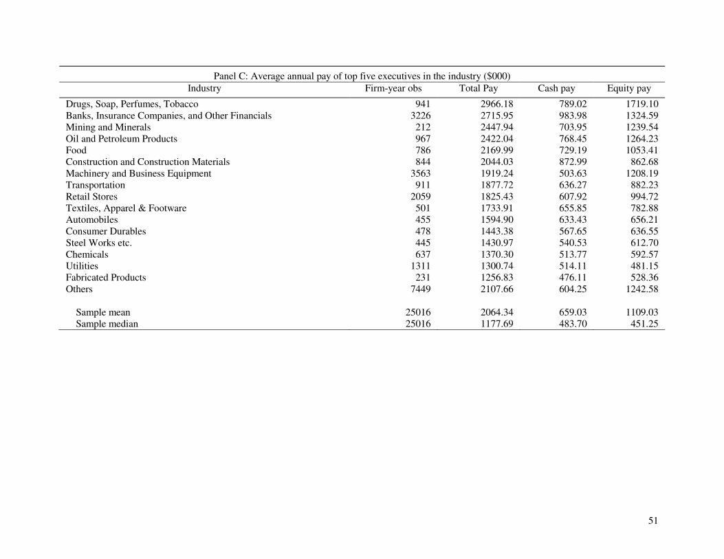
51

Panel C: Average annual pay of top five executives in the industry ($000)

Industry Firm-year obs Total Pay Cash pay Equity pay

Drugs, Soap, Perfumes, Tobacco 941 2966.18 789.02 1719.10 Banks, Insurance Companies, and Other Financials 3226 2715.95 983.98 1324.59 Mining and Minerals 212 2447.94 703.95 1239.54 Oil and Petroleum Products 967 2422.04 768.45 1264.23 Food 786 2169.99 729.19 1053.41 Construction and Construction Materials 844 2044.03 872.99 862.68 Machinery and Business Equipment 3563 1919.24 503.63 1208.19 Transportation 911 1877.72 636.27 882.23 Retail Stores 2059 1825.43 607.92 994.72 Textiles, Apparel & Footware 501 1733.91 655.85 782.88 Automobiles 455 1594.90 633.43 656.21 Consumer Durables 478 1443.38 567.65 636.55 Steel Works etc. 445 1430.97 540.53 612.70 Chemicals 637 1370.30 513.77 592.57 Utilities 1311 1300.74 514.11 481.15 Fabricated Products 231 1256.83 476.11 528.36 Others 7449 2107.66 604.25 1242.58

Sample mean 25016 2064.34 659.03 1109.03 Sample median 25016 1177.69 483.70 451.25

52

Table 3

Geographic Segmentation in Executive Compensation

The annual pay of top 5 executives is regressed on the average annual pay of top 5

executives of other companies in the MSA and control variables. Three regressions are tabulated, separately for the total pay, equity pay and cash pay. Total pay is the sum of salary, bonus, restricted stock grants, stock option grants, long-term incentive payouts and other compensation received by the executive during the year. Cash pay is the sum of salary and bonus while equity pay is the value of stock and option grants received during the year. Control variables include Sales (the logarithm of total sales), the Market-to-book ratio, Cash flow shortfall (the three-year average of the sum of common and preferred dividends plus the cash flow used in investing activities minus the cash flow generated from operations, normalized by total assets), Interest burden (the three-year average of interest expense scaled by operating income before depreciation), R&D (the three-year average of research and development expense scaled by sales), Past one-year stock return (the firm’s stock return in the prior fiscal year), Stock return volatility (the standard deviation of stock returns in the prior fiscal year), ROA (net income divided by total assets), Age (the age of the executive), Tenure (the number of years the executive has worked in the company as a top executive), and the GIM index (the Gompers, Ishii and Metrick (2003) index). All regressions include industry (based on the Fama-French 17 industry classification) and year dummies to control for industry and year fixed effects. ***, ** and * indicate statistical significance at the 1%, 5% and 10% level, respectively. Numbers in parenthesis are t-statistics corrected for clustering at the industry level.

53

Total pay Equity pay Cash pay

Avg. Top5 pay in MSA 0.1868*** 0.1877*** 0.2077*** (7.08) (4.14) (6.78)

Cash flow shortfall -0.4809*** -1.3760*** 0.0770 (5.72) (6.32) (1.36)

Interest burden 0.0289 0.0004 0.0101 (0.90) (0.01) (0.42)

R&D 0.6993*** 1.7927*** 0.2532*** (11.08) (11.21) (7.47)

Age 0.0118 0.0651*** -0.0177*** (1.54) (2.85) (3.09)

Tenure -0.0001 -0.1177*** 0.0374*** (0.01) (6.15) (6.62)

Sales 0.3768*** 0.5452*** 0.2690*** (45.53) (26.37) (43.52)

Market-to-book 0.0443*** 0.0872*** 0.0100*** (12.50) (9.44) (4.85)

Past one-year stock return 0.0967*** 0.1190*** 0.0407*** (8.93) (4.12) (6.67)

Stock return volatility 1.1517*** 1.9825*** -0.1207 (7.51) (4.81) (1.19)

ROA 0.1822* 0.1542 0.3128*** (1.87) (0.59) (4.90)

GIM index 0.0009 0.0124 0.0010 (0.22) (1.21) (0.34)

Adjusted R2 0.508 0.213 0.573 N 15,318 15,277 15,331 Year fixed effect Yes Yes Yes Industry fixed effect Yes Yes Yes

54

Table 4

Local Job Relocations and Executive Compensation

The annual pay of top 5 executives is regressed on the average annual pay of top 5

executives of other companies in the MSA, the high local move dummy, the cross term of the previous two variables, and control variables. Three regressions are tabulated, separately for the total pay, equity pay and cash pay. Total pay is the sum of salary, bonus, restricted stock grants, stock option grants, long-term incentive payouts and other compensation received by the executive during the year. Cash pay is the sum of salary and bonus while equity pay is the value of stock and option grants received during the year. The high local move dummy is 1 for MSAs with the percentage of local job relocations above the sample median for all MSAs and 0 otherwise. Control variables are identical to those used in Table 3. All regressions include industry (based on the Fama-French 17 industry classification) and year dummies to control for industry and year fixed effects. ***, ** and * indicate statistical significance at the 1%, 5% and 10% level, respectively. Numbers in parenthesis are t-statistics corrected for clustering at the industry level.

55

Total Pay Equity Pay Cash Pay

High local move dummy -0.9838*** -0.5792 -0.5759** (3.87) (1.35) (2.23)

(Avg. Top5 pay in MSA)×(High local move dummy) 0.1456*** 0.1124* 0.0972** (4.25) (1.81) (2.43)

Avg. Top5 pay in MSA 0.0652** 0.0867* 0.1154*** (2.25) (1.83) (3.27)

Cash flow shortfall -0.4832*** -1.3812*** 0.0779 (5.76) (6.35) (1.38)

Interest burden 0.0301 0.0003 0.0099 (0.94) (0.00) (0.41)

R&D 0.6997*** 1.8039*** 0.2532*** (11.22) (11.35) (7.66)

Age 0.0123 0.0655*** -0.0176*** (1.61) (2.88) (3.07)

Tenure -0.0007 -0.1186*** 0.0373*** (0.09) (6.20) (6.60)

Sales 0.3746*** 0.5418*** 0.2682*** (45.61) (26.15) (43.71)

Market-to-Book 0.0437*** 0.0864*** 0.0097*** (12.44) (9.40) (4.72)

Past one-year stock return 0.0969*** 0.1189*** 0.0409*** (9.03) (4.14) (6.68)

Stock return volatility 1.1063*** 1.9166*** -0.1386 (7.30) (4.64) (1.38)

ROA 0.1787* 0.1486 0.3134*** (1.84) (0.57) (4.92)

GIM index 0.0019 0.0141 0.0015 (0.48) (1.36) (0.53)

Adjusted R2 0.511 0.215 0.574 N 15,318 15,277 15,331 Year fixed effect Yes Yes Yes Industry fixed effect Yes Yes Yes

56

Table 5

The Local Networking Explanation

The neighborhood surrounding a firm is divided into three non-overlapping regions –

nearby, medium and distant – with increasing geographic distance from the firm. For results reported in Panel A, nearby, medium and distant firms are defined as firms within the same MSA, within the same state but outside the MSA, and in neighboring states, respectively. For results reported in Panel B, medium and distant firms are defined as firms within a 40-mile radius, between 40- and 80-mile radius, and between 80- and 120-mile radium, respectively. The annual pay of top 5 executives is regressed on the average annual pay of top 5 executives of other companies in the nearby, medium, and distant regions, respectively, plus control variables. The three average pay variables are first added to the regression one at a time and then altogether simultaneously. The executive’s total pay is the sum of salary, bonus, restricted stock grants, stock option grants, long-term incentive payouts and other compensation received by the executive during the year. Control variables are identical to those used in Table 3. All regressions include industry (based on the Fama-French 17 industry classification) and year dummies to control for industry and year fixed effects. ***, ** and * indicate statistical significance at the 1%, 5% and 10% level, respectively. Numbers in parenthesis are t-statistics corrected for clustering at the industry level.

57

Panel A: MSA, state and neighboring states

(1) (2) (3) (4)

Avg. Top5 pay in MSA 0.1985*** 0.1249*** (6.87) (3.56)

Avg. Top5 pay in state 0.1760*** 0.1092*** (6.02) (3.03)

Avg. Top5 pay in neighb. state(s) -0.0244 0.0263 (0.52) (0.56)

Cash flow shortfall -0.4781*** -0.4687*** -0.4696*** -0.4757*** (5.51) (5.36) (5.38) (5.46)

Interest burden 0.0222 0.0249 0.0275 0.0233 (0.66) (0.74) (0.81) (0.70)

R&D 0.7078*** 0.6939*** 0.7018*** 0.6996*** (11.18) (11.34) (10.99) (11.27)

Age 0.0107 0.0109 0.0100 0.0110 (1.35) (1.37) (1.25) (1.38)

Tenure -0.0015 -0.0018 -0.0010 -0.0018 (0.19) (0.23) (0.13) (0.23)

Sales 0.3786*** 0.3779*** 0.3809*** 0.3776*** (44.60) (44.34) (43.91) (44.65)

Market-to-book 0.0449*** 0.0446*** 0.0462*** 0.0444*** (12.22) (12.10) (12.48) (12.06)

Past one-year stock return 0.0973*** 0.0972*** 0.0975*** 0.0973*** (8.61) (8.57) (8.51) (8.61)

Stock return volatility 1.1954*** 1.1877*** 1.2568*** 1.1774*** (7.59) (7.49) (7.87) (7.46)

ROA 0.1826* 0.1913* 0.1879* 0.1859* (1.83) (1.92) (1.87) (1.86)

GIM index 0.0014 0.0015 -0.0001 0.0018 (0.36) (0.36) (0.03) (0.44)

Adjusted R2 0.512 0.512 0.506 0.513 N 14,440 14,440 14,440 14,440 Year fixed effect Yes Yes Yes Yes Industry fixed effect Yes Yes Yes Yes

58

Panel B: The 40-, 80-, and 120-mile radius

(1) (2) (3) (4)

Avg. top5 pay within 40 miles 0.1946 0.1729 (6.32)*** (3.86)*** Avg. pay top5 btw 40 and 80 miles 0.0323 0.0001 (0.99) (0.00) Avg. pay top5 btw 80 and 120 miles 0.0391 0.0335 (1.15) (0.80) Cash flow shortfall -0.3997 -0.3146 -0.2858 -0.2690 (3.67)*** (2.49)** (2.27)** (1.84)* Interest burden 0.0504 0.0150 0.0731 0.0497 (1.18) (0.30) (1.41) (0.81) R&D 0.8192 0.8993 0.8867 0.8379 (9.87)*** (10.68)*** (9.21)*** (8.52)*** Age -0.0043 -0.0050 -0.0040 -0.0048 (2.05)** (1.98)** (1.68)* (1.66)* Tenure -0.0042 -0.0043 -0.0013 -0.0005 (1.57) (1.46) (0.49) (0.17) Sales 0.4241 0.4409 0.4534 0.4372 (39.98)*** (39.14)*** (41.67)*** (34.64)*** Market-to-book 0.0394 0.0411 0.0356 0.0347 (8.94)*** (7.94)*** (7.43)*** (6.10)*** Past one-year stock return 0.0904 0.0993 0.1302 0.1447 (5.87)*** (5.46)*** (7.13)*** (6.76)*** Stock return volatility 0.6887 0.9960 0.9833 0.6472 (3.46)*** (4.26)*** (4.13)*** (2.30)** ROA 0.4137 0.5148 0.4447 0.4742 (3.14)*** (3.52)*** (2.70)*** (2.49)** GIM index 0.0075 0.0111 0.0148 0.0113 (1.54) (1.97)** (2.72)*** (1.75)* Adjusted R2 0.423 0.440 0.476 0.471 N 15,016 10,237 10,459 7,363 Year fixed effect Yes Yes Yes Yes Industry fixed effect Yes Yes Yes Yes

59

Table 6

Location Attractiveness and Local Competition for Executive Talents

The average annual pay of the top five executives is regressed on two proxies for cost of living in the MSA (average house

price and ACCRA Cost of Living index), the number of S&P 1500 firms in the MSA, the MSA average of the average annual pay of top five executives of other companies located in the MSA, and control variables. Average house price is the average price of house sales in the MSA. The ACCRA Cost of Living Index is obtained from the Council for Community and Economic Research. The executive’s total pay is the sum of salary, bonus, restricted stock grants, stock option grants, long-term incentive payouts and other compensation received by the executive during the year. Control variables are identical to those used in Table 3. Four versions of the regression are run and tabulated in columns (1)-(4), respectively. All regressions include industry (based on the Fama-French 17 industry classification) and year dummies to control for industry and year fixed effects. ***, ** and * indicate statistical significance at the 1%, 5% and 10% level, respectively. Numbers in parenthesis are t-statistics corrected for clustering at the industry level.

60

(1) (2) (3) (4) (5)

Avg. top5 pay in MSA 0.1228*** 0.1415*** 0.0797*** 0.0714*** 0.0712** (4.05) (5.34) (2.93) (2.63) (2.29)

Cash flow shortfall -0.4925*** -0.4971*** -0.4670*** -0.4751*** -0.4864*** (5.80) (5.90) (5.57) (5.66) (5.74)

Interest burden 0.0367 0.0306 0.0273 0.0282 0.0326 (1.14) (0.96) (0.86) (0.89) (1.02)

R&D 0.6802*** 0.6835*** 0.6431*** 0.6420*** 0.6465*** (11.11) (11.00) (10.35) (10.41) (10.54)

Age 0.0132* 0.0121 0.0100 0.0104 0.0118 (1.73) (1.59) (1.32) (1.36) (1.54)

Tenure -0.0013 -0.0006 0.0008 0.0005 -0.0004 (0.17) (0.08) (0.11) (0.07) (0.05)

Sales 0.3741*** 0.3764*** 0.3760*** 0.3759*** 0.3749*** (45.09) (45.70) (45.51) (45.59) (45.00)

Market-to-book 0.0432*** 0.0435*** 0.0429*** 0.0427*** 0.0424*** (12.10) (12.21) (12.38) (12.27) (12.03)

Past one-year stock return 0.1026*** 0.0982*** 0.0962*** 0.0968*** 0.1018*** (9.61) (9.03) (9.03) (9.06) (9.62)

Stock return volatility 1.1029*** 1.1260*** 1.0070*** 1.0106*** 1.0192*** (7.21) (7.41) (6.64) (6.67) (6.68)

ROA 0.1797* 0.1791* 0.1642* 0.1647* 0.1659* (1.84) (1.84) (1.70) (1.70) (1.71)

GIM index 0.0022 0.0016 0.0045 0.0044 0.0043 (0.55) (0.41) (1.13) (1.12) (1.06)

ACCRA Cost of Living index 0.0057*** 0.0024* 0.0018 (4.44) (1.72) (1.30)

Average house price 0.1023*** 0.0922*** 0.0721*** (7.10) (5.95) (4.02)

# of S&P 1500 firms in MSA 0.0659*** 0.0301** (4.91) (1.97)

Adjusted R2 0.514 0.510 0.515 0.515 0.517 N 15,169 15,318 15,318 15,318 15,169 Year fixed effect Yes Yes Yes Yes Yes Industry fixed effect Yes Yes Yes Yes Yes

61

Table 7

The Role of Management Style

Management style is proxied by the firm’s investment policy (capital expenditure and research and development expenses), financial policy (financial leverage, interest coverage, cash holdings, working capital and dividends) and tax policy (effective tax rate). For each policy variable (e.g., capital expenditure), the regression includes the MSA average of the policy variable, the high local move bias dummy (High local move bias), and control variables (Cash flows, Tobin’s Q, ROA, Assets and TLCF). High local move bias is 1 if the firm is in an MSA with above median local move bias and 0 otherwise. Cash flows is the sum of earnings before extraordinary items and depreciation over lagged total assets. Tobin’s Q is the market value of assets divided by the book value of assets. ROA is earnings before depreciation, interest and tax over lagged total assets. Assets is natural log of total assets. TLCF is a dummy variable for tax-loss carry forward (1 if it is positive and 0 otherwise). All regressions include year and manager dummies to control for year and manager fixed effects. ***, ** and * indicate statistical significance at the 1%, 5% and 10% level, respectively. Numbers in parenthesis are t-statistics corrected for clustering at the firm level.

62

Investment policy Financial policy Operating performance

(1) (2) (3) (4) (5) (6) (7) (8)

Capex R&D Leverage Interest coverage

Cash holdings

Working capital

Dividends ROA

MSA avg 0.0020 0.0343 0.0923** 0.0863** -0.0244 0.0269 -0.0011 -0.0646

(0.04) (1.18) (2.19) (2.04) (0.72) (0.78) (0.06) (1.41)

High local bias dummy 0.0008 -0.0017 0.0038 -0.0273 -0.0046 -0.0078 -0.0002 -0.0182**

(0.14) (0.36) (0.26) (0.12) (0.36) (0.40) (0.02) (2.44)

MSA avg × High local bias dummy 0.0094 0.1108** -0.0338 0.0282 0.1175** 0.0466 -0.0066 0.2670***

(0.12) (2.16) (0.37) (0.32) (2.06) (0.85) (0.24) (3.07)

Cash flows 0.0933*** 0.0076 -0.0276 0.7429** -0.0164 0.0558 -0.0593** 0.1076***

(3.96) (0.48) (1.00) (1.98) (0.38) (1.07) (2.27) (3.42)

Tobin’s Q 0.0104*** 0.0051*** -0.0123*** 0.2585*** 0.0246*** 0.0258*** -0.0014 0.0149***

(9.45) (6.69) (10.21) (8.63) (8.17) (7.55) (1.17) (7.16)

TLCF -0.0064*** -0.0008 0.0057 -0.0901** -0.0000 -0.0059 0.0017 -0.0072*

(2.68) (0.48) (1.35) (2.02) (0.01) (0.83) (0.50) (1.86)

ROA -0.0156 -0.0054 -0.1014*** 1.5536*** 0.0285 0.0834 0.0506

(0.76) (0.35) (3.87) (4.51) (0.62) (1.51) (1.60)

Assets -0.0145*** -0.0295*** 0.0258*** -0.1541*** -0.0574*** -0.0844*** 0.0144*** -0.0145***

(8.47) (13.16) (9.19) (4.67) (12.97) (13.83) (6.75) (5.36)

Adjusted R2 0.699 0.853 0.802 0.778 0.785 0.798 0.693 0.542

N 49,006 52,817 53,740 42,412 52,108 46,085 53,048 53,736

Year fixed effect Yes Yes Yes Yes Yes Yes Yes Yes Manager fixed effect Yes Yes Yes Yes Yes Yes Yes Yes

63

Table 8

Manager Fixed Effects and Geographic Variations in Executive Compensation

Using a subsample of top executives who have changed firms, we re-estimate the annual pay regression by controlling for manager fixed effects. Each executive’s annual pay is regressed on the average annual pay of top executives of other firms in the MSA, with or without control for unobservable manager fixed effects. The regression results are tabulated, separately for the executive’s total annual pay, annual equity pay and annual cash pay. Total pay is the sum of salary, bonus, restricted stock grants, stock option grants, long-term incentive payouts and other compensation received by the executive during the year. Cash pay is the sum of salary and bonus while equity pay is the value of stock and option grants received during the year. Control variables are identical to those used in Table 3. All regressions include industry (based on the Fama-French 17 industry classification) and year dummies to control for industry and year fixed effects. ***, ** and * indicate statistical significance at the 1%, 5% and 10% level, respectively. Numbers in parenthesis are t-statistics corrected for clustering at the industry level.

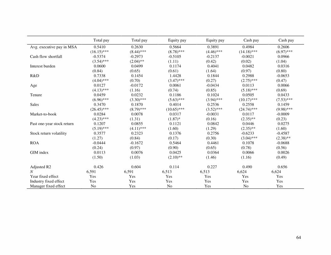
64

Total pay Total pay Equity pay Equity pay Cash pay Cash pay

Avg. executive pay in MSA 0.5410 0.2630 0.5664 0.3891 0.4984 0.2606 (16.15)*** (8.44)*** (8.78)*** (4.46)*** (14.18)*** (6.97)*** Cash flow shortfall -0.5374 -0.2973 -0.5105 -0.2137 -0.0021 0.0966 (3.54)*** (2.04)** (1.11) (0.42) (0.02) (1.04) Interest burden 0.0600 0.0499 0.1174 0.4041 0.0482 0.0316 (0.84) (0.65) (0.61) (1.64) (0.97) (0.80) R&D 0.7338 0.1454 1.4428 0.1844 0.2988 -0.0653 (4.04)*** (0.70) (3.47)*** (0.27) (2.75)*** (0.47) Age 0.0127 -0.0172 0.0061 -0.0434 0.0113 0.0066 (4.13)*** (1.16) (0.74) (0.85) (5.18)*** (0.69) Tenure 0.0459 0.0232 0.1186 0.1024 0.0505 0.0433 (6.96)*** (3.30)*** (5.63)*** (3.94)*** (10.17)*** (7.53)*** Sales 0.3470 0.1870 0.4014 0.2536 0.2558 0.1459 (26.45)*** (8.79)*** (10.65)*** (3.52)*** (24.74)*** (9.98)*** Market-to-book 0.0284 0.0078 0.0317 -0.0031 0.0117 -0.0009 (4.23)*** (1.31) (1.87)* (0.16) (2.35)** (0.23) Past one-year stock return 0.1207 0.0855 0.1121 0.0842 0.0446 0.0275 (5.19)*** (4.11)*** (1.60) (1.29) (2.35)** (1.60) Stock return volatility 0.3577 0.2323 0.1376 0.2756 -0.6233 -0.4587 (1.27) (0.84) (0.17) (0.30) (3.04)*** (2.38)** ROA -0.0444 -0.1672 0.5464 0.4461 0.1078 -0.0688 (0.24) (0.97) (0.90) (0.65) (0.78) (0.56) GIM index 0.0113 0.0076 0.0425 0.0364 0.0066 0.0026 (1.50) (1.03) (2.10)** (1.46) (1.16) (0.49) Adjusted R2 0.426 0.604 0.114 0.227 0.490 0.656 N 6,591 6,591 6,513 6,513 6,624 6,624 Year fixed effect Yes Yes Yes Yes Yes Yes Industry fixed effect Yes Yes Yes Yes Yes Yes Manager fixed effect No Yes No Yes No Yes

65

Table 9

Geographic Variation in Management Styles and Manager Fixed Effects

Using a subsample of top executives who have changed firms, we re-estimate the management style regressions as in Bertrand and Schoar (2003). For each management style regression we extract the manager fixed effects (MFEs) and then compute the average MSA-MFE. Each executive’s MFE is then regressed on the average annual MSA-MFE interacted with whether the MSA is classified as a high- or low- local bias MSA. High local move bias is 1 if the firm is in an MSA with above median local move bias and 0 otherwise. Cash flows is the sum of earnings before extraordinary items and depreciation over lagged total assets. Tobin’s Q is the market value of assets divided by the book value of assets. ROA is earnings before depreciation, interest and tax over lagged total assets. Assets is natural log of total assets. TLCF is a dummy variable for tax-loss carry forward (1 if it is positive and 0 otherwise). All regressions include industry (based on the Fama-French 17 industry classification) and year dummies to control for industry and year fixed effects. ***, ** and * indicate statistical significance at the 1%, 5% and 10% level, respectively. Numbers in parenthesis are t-statistics clustered at the executive level. t-stats for the difference in coefficients between high and low bias average MSA-MFEs is also shown.

Variables (ROA) (RD) (CAPEX) (LEVG) (IC) (CASH) (WC) (DIV) (ETX)

MFE MSA*Low bias 0.3179*** 0.4798*** 0.1316** 0.1709*** -0.0824 0.4135*** 0.2832*** 0.0862 0.0544 (5.73) (7.87) (2.23) (2.70) (1.34) (6.91) (5.02) (1.64) (0.90) MFE MSA*High bias 0.7044*** 0.9433*** 0.3637*** 0.6374*** 0.5471*** 0.9217*** 0.7459*** 0.6332*** 0.3346*** (7.40) (16.46) (2.81) (9.25) (6.47) (15.62) (9.19) (7.63) (3.60)

t-stat for diff (3.68)*** (5.78)*** (1.63) (5.06)*** (6.15)*** (6.19)*** (4.73)*** (5.60)*** (2.54)*** Adjusted R2 0.057 0.296 0.019 0.041 0.029 0.238 0.085 0.043 0.008 N 7,194 7,196 6,950 7,196 6,124 7,047 6,776 7,176 6,968

66

Table 10

Local Beta and Stock Option Grants

The executive’s annual stock option grant is regressed on the firm’s local beta and control

variables. The size of a stock option grant is measured as the total number of options in the grant scaled by total shares outstanding. Local beta is estimated by regressing the firm’s monthly stock returns against the monthly average stock returns of other firms in the MSA, the monthly market returns and the industry stock index returns. Control variables include Sales (the logarithm of total sales), the Book-to-market ratio, Cash flow shortfall (the three-year average of the sum of common and preferred dividends plus the cash flow used in investing activities minus the cash flow generated from operations, normalized by total assets), Interest burden (the three-year average of interest expense scaled by operating income before depreciation), R&D (the three-year average of research and development expense scaled by sales), Long-term debt dummy (1 if the firm has long-term debt outstanding and 0 otherwise), Low marginal tax dummy (1 if the firm has negative taxable income and net operating loss carry-forwards in each of the prior three years and 0 otherwise), High marginal tax dummy (1 if the firm has positive taxable income and no net operating loss carry-forwards in each of the prior three years and 0 otherwise), Employees (the logarithm of the number of employees), Past one-year stock return (the firm’s stock return in the prior fiscal year), Stock return volatility (the standard deviation of stock returns in the prior fiscal year), Operating loss dummy (1 if the firm reported negative earnings in the fiscal year and 0 otherwise), Tight labor market dummy (1 if the unemployment rate for the year in the MSA exceeds the average unemployment rate for the MSA during the sample period and 0 otherwise), Non-compete enforceability index (extracted from Garmaise (2006)), Median abnormal returns for MSA (median abnormal returns for all firms in the MSA in the prior year), MSA education (percentage of MSA population with at least a bachelor’s degree), High education dummy (1 if the fraction of the MSA population with a bachelor’s degree is in the top quartile), and Highest income tax rate for state (the highest state income tax rate during the year). All regressions include industry (based on the Fama-French 17 industry classification) and year dummies to control for industry and year fixed effects. ***, ** and * indicate statistical significance at the 1%, 5% and 10% level, respectively. Numbers in parenthesis are t-statistics corrected for clustering at the industry level.

67

(1) (2)

Cash flow shortfall 0.0017 0.0017 (2.60)*** (2.62)*** Interest burden 0.0002 0.0002 (0.65) (0.64) R&D -0.0015 -0.0016 (3.28)*** (3.28)*** Book-to-market 0.0009 0.0009 (3.91)*** (3.92)*** Long-term debt dummy -0.0000 -0.0000 (0.05) (0.04) Low marginal tax dummy 0.0002 0.0002 (0.21) (0.20) High marginal tax dummy -0.0005 -0.0005 (3.44)*** (3.44)*** Sales -0.0007 -0.0007 (6.29)*** (6.29)*** Employees -0.0003 -0.0003 (1.93)* (1.93)* Past one-year stock return -0.0003 -0.0003 (2.37)** (2.37)** Stock return volatility 0.0087 0.0087 (6.42)*** (6.41)*** Operating loss dummy 0.0003 0.0003 (1.03) (1.03) Tight labor market dummy -0.0000 -0.0000 (0.17) (0.20) Local MSA beta 0.0006 0.0006 (3.17)*** (3.16)*** Non-compete enforceability index -0.0001 -0.0001 (1.68)* (1.65)* Median abnormal returns for MSA 0.0003 0.0003 (1.29) (1.27) MSA education -0.0000 -0.0000 (0.08) (0.13) High education dummy 0.0003 0.0002 (1.15) (0.49) Highest income tax rate for state -0.0000 -0.0000 (0.59) (0.58) Option grants of other firms in MSA 0.0153 0.0058 (0.46) (0.15) (High education dummy)× (Option grants of other firms in MSA) 0.0277 (0.41) Adjusted R2 0.205 0.205 N 10,072 10,072 Year fixed effect Yes Yes Industry fixed effect Yes Yes

68

Table 11

Location Effects on CEO Compensation

CEO pay is regressed against the average pay of other CEOs in the MSA and control

variables. Three regressions are tabulated, separately for the CEO’s total pay, equity pay and cash pay. Total pay is the sum of salary, bonus, restricted stock grants, stock option grants, long-term incentive payouts and other compensation received by the CEO during the year. Cash pay is the sum of salary and bonus while equity pay is the value of stock and option grants received during the year. The average CEO pay in the MSA is calculated by removing the CEO’s own pay from the average. Control variables are similar to those used in Table 3. All regressions include industry (based on the Fama-French 17 industry classification) and year dummies to control for industry and year fixed effects. ***, ** and * indicate statistical significance at the 1%, 5% and 10% level, respectively. Numbers in parenthesis are t-statistics corrected for clustering at the industry level.

69

Total pay Equity pay Cash pay

Avg. CEO pay in MSA 0.1610 0.1128 0.1898 (5.69)*** (1.87)* (5.67)*** Cash flow shortfall -0.3594 -0.9191 0.1577 (3.28)*** (2.74)*** (1.75)* Interest burden 0.0282 0.0139 0.0050 (0.68) (0.11) (0.16) R&D 0.7149 1.9545 0.2584 (9.35)*** (8.23)*** (5.35)*** Age -0.0061 -0.0439 0.0026 (3.00)*** (6.44)*** (1.57) Tenure -0.0059 -0.0433 0.0057 (2.15)** (5.34)*** (2.64)*** Sales 0.4029 0.5948 0.2757 (37.36)*** (18.10)*** (31.12)*** Market-to-book 0.0380 0.0679 0.0044 (8.66)*** (4.95)*** (1.60) Past one-year stock return 0.0833 0.0542 0.0435 (5.58)*** (1.19) (4.58)*** Stock return volatility 0.6656 0.3391 -0.7926 (3.35)*** (0.54) (5.44)*** ROA 0.3305 0.3183 0.5672 (2.49)** (0.78) (5.85)*** GIM index 0.0050 0.0402 0.0070 (1.03) (2.56)** (1.85)* Adjusted R2 0.417 0.142 0.429 N 15,100 15,079 15,118 Year fixed effect Yes Yes Yes Industry fixed effect Yes Yes Yes