Job Polarization and Structural Change∗

Zsofia L. Barany† Christian Siegel‡

April 2014

Abstract

Job polarization is a widely documented phenomenon in developed countries since the 1980s:

employment has been shifting from middle to low- and high-income workers, while average wage

growth has been slower for middle-income workers than at both extremes. We document 1) that po-

larization has started as early as the 1950s in the US, and 2) that this process is closely linked to the

shift from manufacturing to services. Based on these observations we propose a structural change

driven explanation for polarization. Productivity growth through raising national income leads to a

disproportionate increase in the demand for high-end (luxury) services. To attract more workers into

the high-skilled services, the wages in this sector have to grow at a faster pace than in the middle. The

growing income of the wealthier part of the population in turn increases their demand for low-skilled

services, leading to a partial marketization of home production, and a faster growth of the low-skilled

service wages.

JEL codes: E24, J22, O41

Keywords: Job Polarization, Structural Change, Home Production

∗We wish to thank Francesco Caselli, Davd Dorn, Per Krusell, Silvana Tenreyro and Akos Valentinyi as well as seminarand conference participants at Trinity College Dublin, UC Berkeley, Sciences Po, Exeter, the 7th Nordic Summer Symposiumin Macroeconomics, the European Meeting of the Econometric Society in Gothenburg, the 2013 Cologne Workshop on Macroeco-nomics, the 2013 Winter Meeting of the Hungarian Society of Economists and the Christmas Meetings of the German EconomistsAbroad in Konstanz for useful comments.†Sciences Po. Email: zsofia.barany@sciencespo.fr‡University of Exeter. Email: c.siegel@exeter.ac.uk

1

1 Introduction

The polarization of the labor market in terms of occupations is a widely documented phenomenon in

the US and several European countries since the 1980s (Autor, Katz, and Kearney (2006), Goos and Man-

ning (2007), and Goos, Manning, and Salomons (2009)). This phenomenon, besides the relative growth

of wages and employment of high earning occupations, also entails the relative growth of wages and

employment of low earning occupations. The leading explanation for polarization is the routinization

hypothesis, which relies on the assumption that information and computer technologies (ICT) substi-

tute for middle-skill and hence middle-earnings (routine) occupations, whereas they complement the

high-skilled and high-earnings (abstract) occupations (Autor, Levy, and Murnane (2003), Autor, Katz,

and Kearney (2006), Michaels, Natraj, and Van Reenen (2010), Goos, Manning, and Salomons (2011),

Autor and Dorn (2012)).

The contribution of our paper is twofold. First, we document a set of facts which raise flags that rou-

tinization, although certainly playing a role from the 1980s onwards, is not the sole driving force behind

this phenomenon. Second, based on these facts we propose a novel perspective on the polarization of

the labor market, one based on structural change.

Our analysis of US Census data for the period 1950-2000 and American Community Survey (ACS)

data for 2008 reveals some novel facts. First, while most of the literature on polarization focuses on

occupations, we document that labor market polarization is present also in terms of broadly defined

sectors: low-skilled and high-skilled service workers, who are at opposite ends of the earnings distri-

bution have been gaining in terms of wages and employment at the expense of manufacturing workers.

Second, we show that the loss in routinizable occupations is not uniform across sectors: routinizable

employment only declined in the manufacturing sector. Third, we find that polarization has started

as early as the 1950-1960s in the US. This implies that polarization started long before ICT or increased

trade flows could have impacted the labor market. Observing a) that polarization seems to be a long-run

phenomenon, b) that the middle earning jobs are in manufacturing, c) that manufacturing employment

started to fall, while service employment started to increase in the 1950s-1960s, it is natural to investi-

gate whether the structural shift of the economy is driving the polarization of the labor market.

Based on these observations we propose a structural change driven explanation for the joint polar-

ization of wages and employment. In our dynamic general equilibrium model workers with heteroge-

neous ability select which sector to work in. As technology improves, the demand for both high- and

low-skilled services increases disproportionately, which leads to a reallocation of labor from middle-

earning manufacturing jobs to high-earning and low-earning service jobs. However, to attract more

workers into these two sectors, the wages in these two sectors have to grow at a faster pace than in the

middle. Finally, we calibrate the model and quantitatively assess the contribution of structural change –

driven by both non-homothetic preferences and unbalanced technological progress – to the polarization

of wages and employment.

In the model, there are two types of consumption goods: manufacturing and high-end service goods.

2

Preferences over these two goods are non-homothetic: high-end services are luxury goods, which are

only demanded at high enough income levels. Additionally a subsistence level of home production

is required, which can be self-produced or acquired on the market. We model low-skilled service jobs

as substitutes for household production. As technology progresses in the consumption goods sector,

the employment and production structure of the economy changes: as households gradually become

wealthier, the demand for high-skilled services rises over-proportionally due to the non-homotheticity

of preferences. This disproportionate demand rise puts an upward pressure on prices and wages in the

high-skilled service sector. Consequently, more people acquire education and work in high-end service

jobs. As wages increase, more and more people decide to hire low-skilled household workers, instead

of doing the housework themselves. This puts an upward pressure on wages at the bottom-end of the

distribution, increasing the supply of these workers. Due to the non-homotheticity of preferences, the

timing of the expansion of the high- and the low-skilled service sector can be different. While the non-

homotheticity is relatively important, the desire to expand the consumption of high-skilled services

dominates that of low-skilled services. This can be a potential explanation of the low-skilled service

expansion becoming more pronounced later on in the data.

This paper builds on and contributes to the literature both on polarization and on structural change.

To our knowledge, these two phenomena until now have been studied separately. However, according

to our analysis of the data, polarization of the labor market and structural change are closely linked to

each other, and according to our model, industrial shifts can lead to polarization.

The structural change literature has documented for several countries that as income increases re-

sources are shifted away from agriculture and from manufacturing towards services (Kuznets (1957),

Maddison (1980)). In particular the employment share of manufacturing has been declining since the

1950s, while the employment share of services has been increasing. The literature has identified two

economic forces that lead to structural transformation: preferences and technology. The preferences

explanation relies on changes in aggregate income, which if preferences for the output of different

sectors are not homothetic lead to a reallocation of resources across sectors (Caselli and Coleman II.

(2001), Kongsamut et al (2001)). The technology explanation assumes that productivity growth is dif-

ferent across sectors, which with regular preferences leads to a shift of labor into the lower growth

sector (Ngai and Pissarides (2007), Acemoglu and Guerrieri (2008)). The consensus seems to be that

both mechanisms together are needed to explain the patterns observed in the data (Buera and Kaboski

(2009), Herrendorf et al (2013), Boppart (2011)). Several papers have also established the importance of

home production for structural transformation (Ngai and Pissarides (2008), Buera and Kaboski (2009),

(2012a), (2012b)). In our model we rely on both mechanisms, and incorporate home production.

We extend the structural change literature in two ways. First, we allow heterogeneous workers

to endogenously sort into different skill groups and into jobs in different sectors. In the presence of

differential productivity or demand growth, the optimal education decisions naturally change. Since

the adjustment of the skill supply takes place gradually, it is possible, that wages increase more initially,

3

while later on employment reallocation is more pronounced. Moreover, as the supply of skills and

the sorting into sectors change, the relative wages and prices are affected. Therefore, we can analyze

the effects of structural change on relative sectoral wages, which is not usual in models of structural

change.1

Second, based on the job polarization phenomenon we distinguish between two types of services: low-

and high-skilled. This is an important distinction, due to both the way they enter the utility of agents

and the way they are produced. We believe that consumers enjoy these services in different ways.

We model low-skilled services as substitutes for household production. In the data we do not find a

clear pattern for the total amount of household production – the combined hours of home production

and low-skilled service workers. Therefore, we assume that there is a fixed demand for household

production, which implies an upper limit on the demand for low-skilled services. The demand for

high-skilled services, on the other hand, can increase without bounds. In terms of production, high-

skilled services need specialized (educated) workers, while low-skilled services can be supplied by

anyone.

Two popular explanations suggested for the polarization of occupations are the routinization hy-

pothesis, and the consumption hypothesis. The routinization hypothesis relies on the assumption that

information and computer technologies (ICT) substitute for middle-skill and hence middle-earnings

(routine) occupations, whereas they complement the high-skilled and high-earnings (abstract) occu-

pations (Autor, Levy, and Murnane (2003), Autor, Katz, and Kearney (2006), Michaels, Natraj, and

Van Reenen (2010), Goos, Manning, and Salomons (2011), Autor and Dorn (2012)). It has been argued

that much of the expansion of low-skilled occupations is driven by the expansion of low-skilled ser-

vice jobs (Autor and Dorn (2012)). The routinization hypothesis suggests, that it is ICT that leads to

the substitution of routine workers by machines, and which complements abstract workers. The dis-

placed routine workers find either abstract or manual jobs, increasing the employment share of these

occupations (Autor, Levy, and Murnane (2003), Autor, Katz, and Kearney (2006), Michaels, Natraj, and

Van Reenen (2010), Goos, Manning, and Salomons (2011)). The routinization hypothesis, linked to ICT,

is potentially a convincing explanation for the employment share patterns after the mid-1980s, but with-

out any assumption on demands, it does not provide a mechanism through which the relative wage of

manual workers compared to routine workers can increase. It also cannot provide an explanation for

the patterns observed before ICT could have taken effect. The consumption spill-over argument, on

the other hand, suggests that as the income of high-earners increases, their demand for low-skilled ser-

vice jobs increases as well, leading to a spillover to the lower end of the wage distribution (Manning

(2004), Mazzolari and Ragusa (2007)). Our modeling of low-skilled service jobs as substitutes for home

production is reminiscent of this argument.

1A notable exception is Caselli and Coleman II. (2001).

4

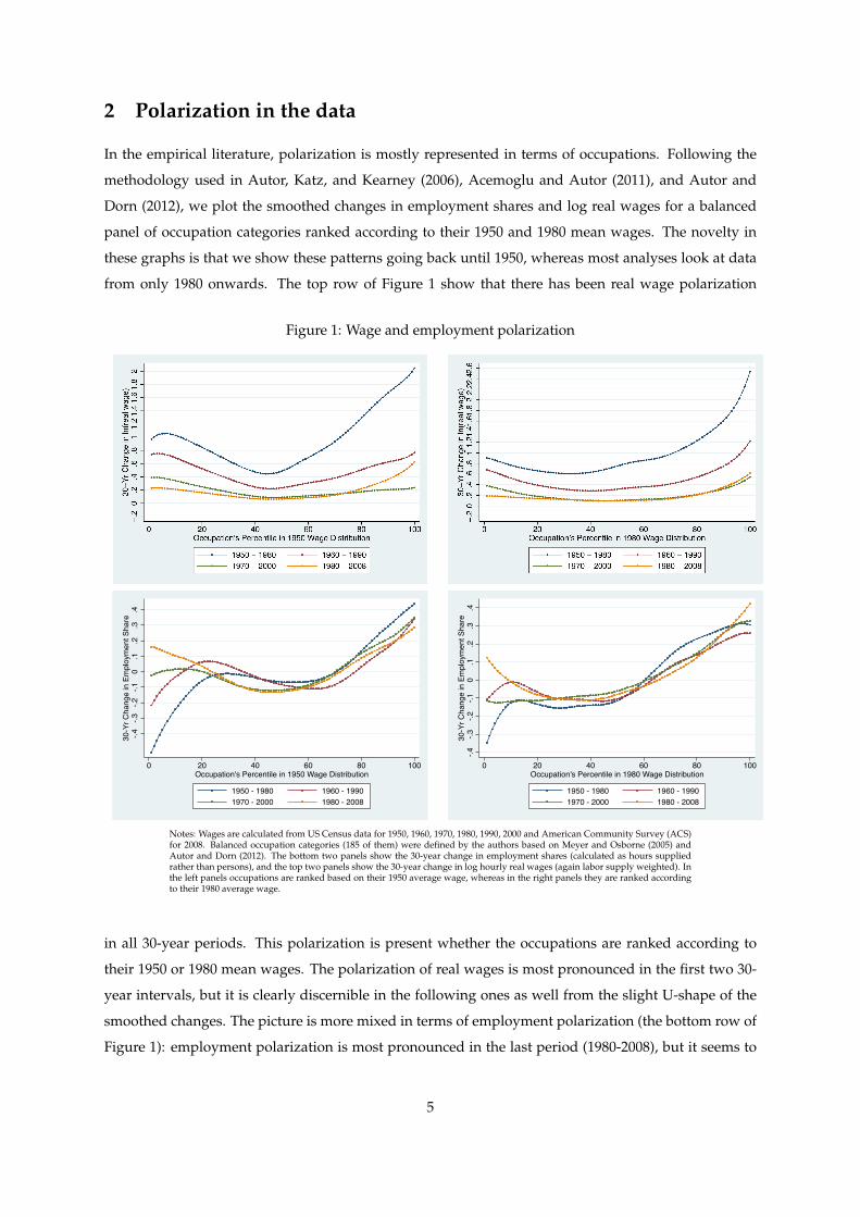
2 Polarization in the data

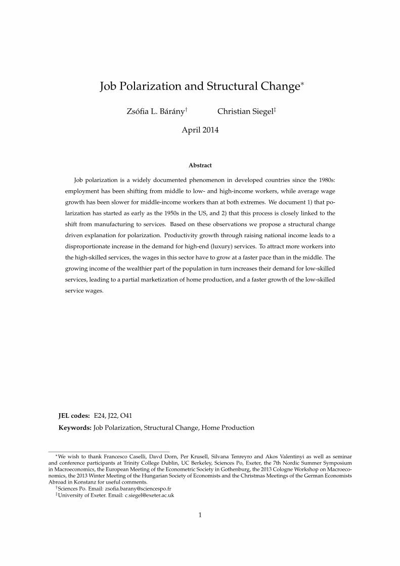
In the empirical literature, polarization is mostly represented in terms of occupations. Following the

methodology used in Autor, Katz, and Kearney (2006), Acemoglu and Autor (2011), and Autor and

Dorn (2012), we plot the smoothed changes in employment shares and log real wages for a balanced

panel of occupation categories ranked according to their 1950 and 1980 mean wages. The novelty in

these graphs is that we show these patterns going back until 1950, whereas most analyses look at data

from only 1980 onwards. The top row of Figure 1 show that there has been real wage polarization

Figure 1: Wage and employment polarization

-.4-.3

-.2-.1

0.1

.2.3

.430

-Yr C

hang

e in

Em

ploy

men

t Sha

re

0 20 40 60 80 100Occupation's Percentile in 1950 Wage Distribution

1950 - 1980 1960 - 19901970 - 2000 1980 - 2008

-.4-.3

-.2-.1

0.1

.2.3

.430

-Yr C

hang

e in

Em

ploy

men

t Sha

re

0 20 40 60 80 100Occupation's Percentile in 1980 Wage Distribution

1950 - 1980 1960 - 19901970 - 2000 1980 - 2008

Notes: Wages are calculated from US Census data for 1950, 1960, 1970, 1980, 1990, 2000 and American Community Survey (ACS)for 2008. Balanced occupation categories (185 of them) were defined by the authors based on Meyer and Osborne (2005) andAutor and Dorn (2012). The bottom two panels show the 30-year change in employment shares (calculated as hours suppliedrather than persons), and the top two panels show the 30-year change in log hourly real wages (again labor supply weighted). Inthe left panels occupations are ranked based on their 1950 average wage, whereas in the right panels they are ranked accordingto their 1980 average wage.

in all 30-year periods. This polarization is present whether the occupations are ranked according to

their 1950 or 1980 mean wages. The polarization of real wages is most pronounced in the first two 30-

year intervals, but it is clearly discernible in the following ones as well from the slight U-shape of the

smoothed changes. The picture is more mixed in terms of employment polarization (the bottom row of

Figure 1): employment polarization is most pronounced in the last period (1980-2008), but it seems to

5

be present even in the earlier decades.2

These graphs – in line with the literature – plot the change in raw employment shares and in raw

log real hourly wages. These changes also include the potential effects of the changing gender, age

and race composition of the labor force. These graphs also do not directly relate to the explanations put

forward in the literature, as they show the employment share and wage changes for occupations ranked

according to their mean wage, not based on their routinizability. Therefore we classify the occupation

groups into the following categories: manual, routine, and abstract (as in Acemoglu et al (2011)), and

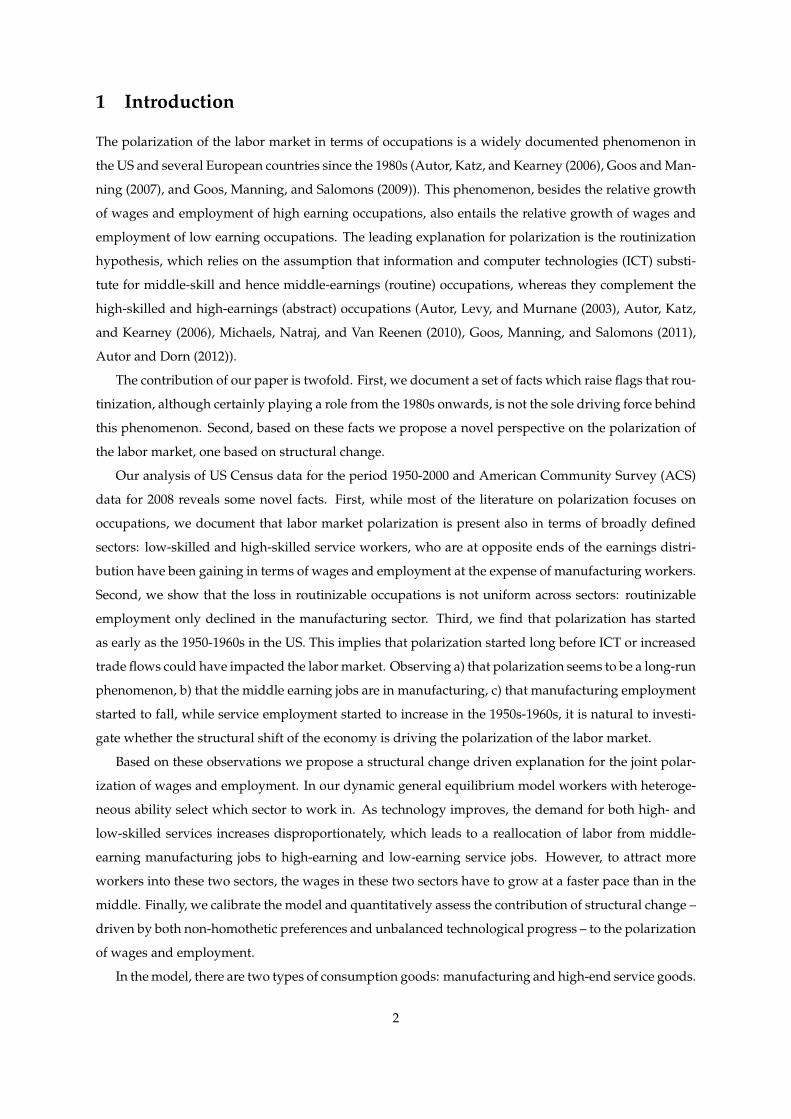
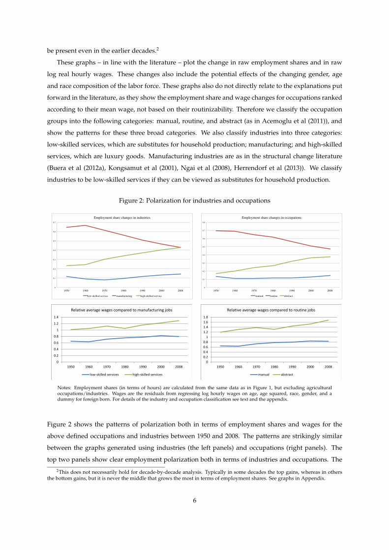
show the patterns for these three broad categories. We also classify industries into three categories:

low-skilled services, which are substitutes for household production; manufacturing; and high-skilled

services, which are luxury goods. Manufacturing industries are as in the structural change literature

(Buera et al (2012a), Kongsamut et al (2001), Ngai et al (2008), Herrendorf et al (2013)). We classify

industries to be low-skilled services if they can be viewed as substitutes for household production.

Figure 2: Polarization for industries and occupations

0

0.1

0.2

0.3

0.4

0.5

0.6

0.7

1950 1960 1970 1980 1990 2000 2008

Employment share changes in industries

low-skilled service manufacturing high-skilled service

0

0.1

0.2

0.3

0.4

0.5

0.6

0.7

0.8

1950 1960 1970 1980 1990 2000 2008

Employment share changes in occupations

manual routine abstract

0

0.2

0.4

0.6

0.8

1

1.2

1.4

1950 1960 1970 1980 1990 2000 2008

Relative average wages compared to manufacturing jobs

low-skilled services high-skilled services

0

0.2

0.4

0.6

0.8

1

1.2

1.4

1.6

1.8

1950 1960 1970 1980 1990 2000 2008

Relative average wages compared to routine jobs

manual abstract

Notes: Employment shares (in terms of hours) are calculated from the same data as in Figure 1, but excluding agriculturaloccupations/industries. Wages are the residuals from regressing log hourly wages on age, age squared, race, gender, and adummy for foreign born. For details of the industry and occupation classification see text and the appendix.

Figure 2 shows the patterns of polarization both in terms of employment shares and wages for the

above defined occupations and industries between 1950 and 2008. The patterns are strikingly similar

between the graphs generated using industries (the left panels) and occupations (right panels). The

top two panels show clear employment polarization both in terms of industries and occupations. The

2This does not necessarily hold for decade-by-decade analysis. Typically in some decades the top gains, whereas in othersthe bottom gains, but it is never the middle that grows the most in terms of employment shares. See graphs in Appendix.

6

middle earning group (manufacturing/routine occupations) lost significantly in terms of employment

share, the top (high-skilled services/abstract) gained, and the bottom (low-skilled services/manual)

initially shrank, but then expanded. The bottom two panels show the change in average industry (or

occupation) log hourly wage change in the given decade compared to the mean log hourly wage change

in manufacturing (or routine occupations). In most decades average wages in low- and high-skilled

services improved relative to manufacturing, while manual and abstract occupations also improved

relative to routine occupations. Exceptions are the first and last decade, and the period between 1970-

1980, when the high-skilled services and the abstract occupations lost. In this decade there was a secular

compression in the skill premium, most probably due to forces outside the scope of this model.3

This striking similarity in the employment share and average wage path of the three broad indus-

try and occupation classifications can be understood when considering the employment shares of the

occupation categories in the three industry categories and vice versa. The top panel in Table 1 shows

the employment shares in each industry-occupation cell. It can be seen that the largest numbers are on

the diagonal, implying there is a tight correspondence between industries an occupations. The middle

panel shows for each industry the fraction of employment coming from manual, routine and abstract

occupations, while the bottom panel shows the opposite averaged between 1950-2008. The majority of

workers in low-skilled services are in manual occupations, the majority in manufacturing are in rou-

tine occupations, and the majority in high-skilled services are in abstract occupations. The opposite is

also true: the majority of routine workers are employed in manufacturing, and the majority of abstract

workers are employed in the high-skilled service industry.

Table 1: Overlap in employment between industry and occupationlow-skilled service manufacturing high-skilled service total

manual 5.90 1.26 5. 17 12.33routine 3.31 44.61 11.78 59.70abstract 1.89 9.05 17.04 27.97total 11.09 54.92 33.99 100manual 53.66 2.30 15.49 -routine 30.07 80.71 35.66 -abstract 16.27 16.98 48.84 -total 100 100 100 -manual 48.37 10.55 41.08 100routine 5.80 74.67 19.53 100abstract 6.44 34.72 58.84 100

Notes: Employment shares (in terms of hours) as percents are calculated from the same data as in Figure 1, but excluding agricul-tural occupations/industries. Industry and occupation classification same as in Figure 2. The top panel shows the employmentshares in each of the occupation-industry cells. The middle panel shows within each industry the employment share of differentoccupations, while the bottom panel shows within each occupation group the employment share of different industries.

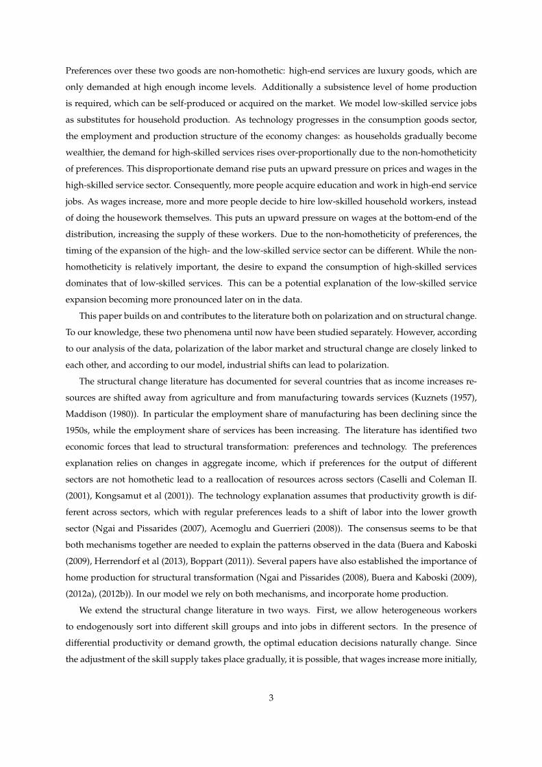
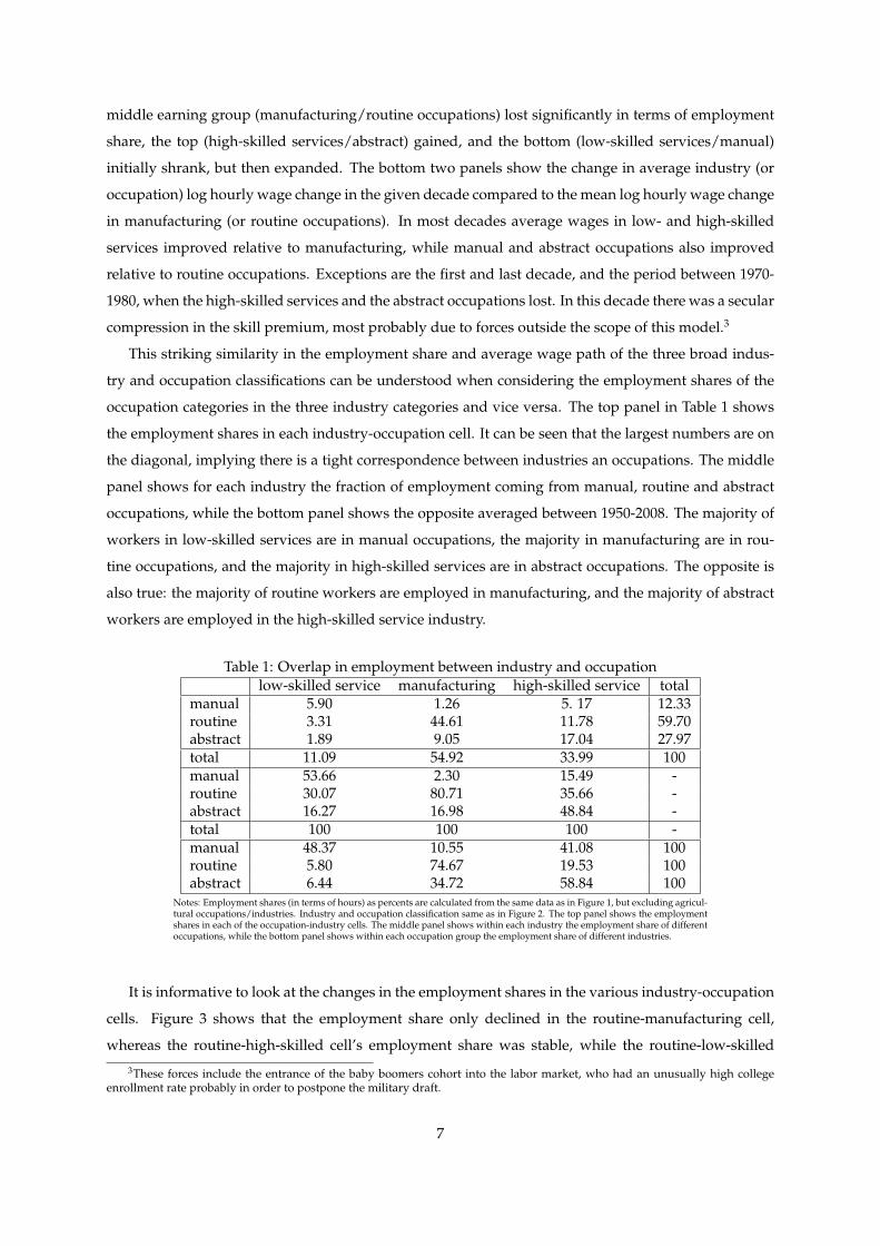
It is informative to look at the changes in the employment shares in the various industry-occupation

cells. Figure 3 shows that the employment share only declined in the routine-manufacturing cell,

whereas the routine-high-skilled cell’s employment share was stable, while the routine-low-skilled

3These forces include the entrance of the baby boomers cohort into the labor market, who had an unusually high collegeenrollment rate probably in order to postpone the military draft.

7

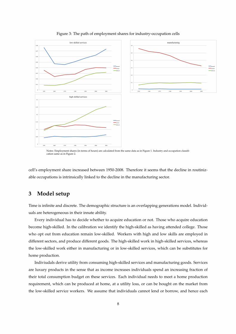
Figure 3: The path of employment shares for industry-occupation cells

0

0.01

0.02

0.03

0.04

0.05

0.06

0.07

0.08

1950 1960 1970 1980 1990 2000 2008

low-skilled services

manual

routine

abstract

0

0.1

0.2

0.3

0.4

0.5

0.6

1950 1960 1970 1980 1990 2000 2008

manufacturing

manual

routine

abstract

0

0.05

0.1

0.15

0.2

0.25

0.3

1950 1960 1970 1980 1990 2000 2008

high-skilled services

manual

routine

abstract

Notes: Employment shares (in terms of hours) are calculated from the same data as in Figure 1. Industry and occupation classifi-cation same as in Figure 2.

cell’s employment share increased between 1950-2008. Therefore it seems that the decline in routiniz-

able occupations is intrinsically linked to the decline in the manufacturing sector.

3 Model setup

Time is infinite and discrete. The demographic structure is an overlapping generations model. Individ-

uals are heterogeneous in their innate ability.

Every individual has to decide whether to acquire education or not. Those who acquire education

become high-skilled. In the calibration we identify the high-skilled as having attended college. Those

who opt out from education remain low-skilled. Workers with high and low skills are employed in

different sectors, and produce different goods. The high-skilled work in high-skilled services, whereas

the low-skilled work either in manufacturing or in low-skilled services, which can be substitutes for

home production.

Indiviudals derive utility from consuming high-skilled services and manufacturing goods. Services

are luxury products in the sense that as income increases individuals spend an increasing fraction of

their total consumption budget on these services. Each individual needs to meet a home production

requirement, which can be produced at home, at a utility loss, or can be bought on the market from

the low-skilled service workers. We assume that individuals cannot lend or borrow, and hence each

8

individual spends all income in the period that it is earned.

The economy is in a decentralized equilibrium at all times: individuals make educational decisions

and sectoral choices to maximize their expected discounted lifetime utility, where in each period they

maximize their utility by optimally allocating their income between low-skilled services, manufacturing

goods and high-skilled services. Production is perfectly competitive, wages and prices are such that

all markets clear. We analyze the role of technological progress and non-homothetic preferences in

explaining the observed wage and employment dynamics since the 1950s.

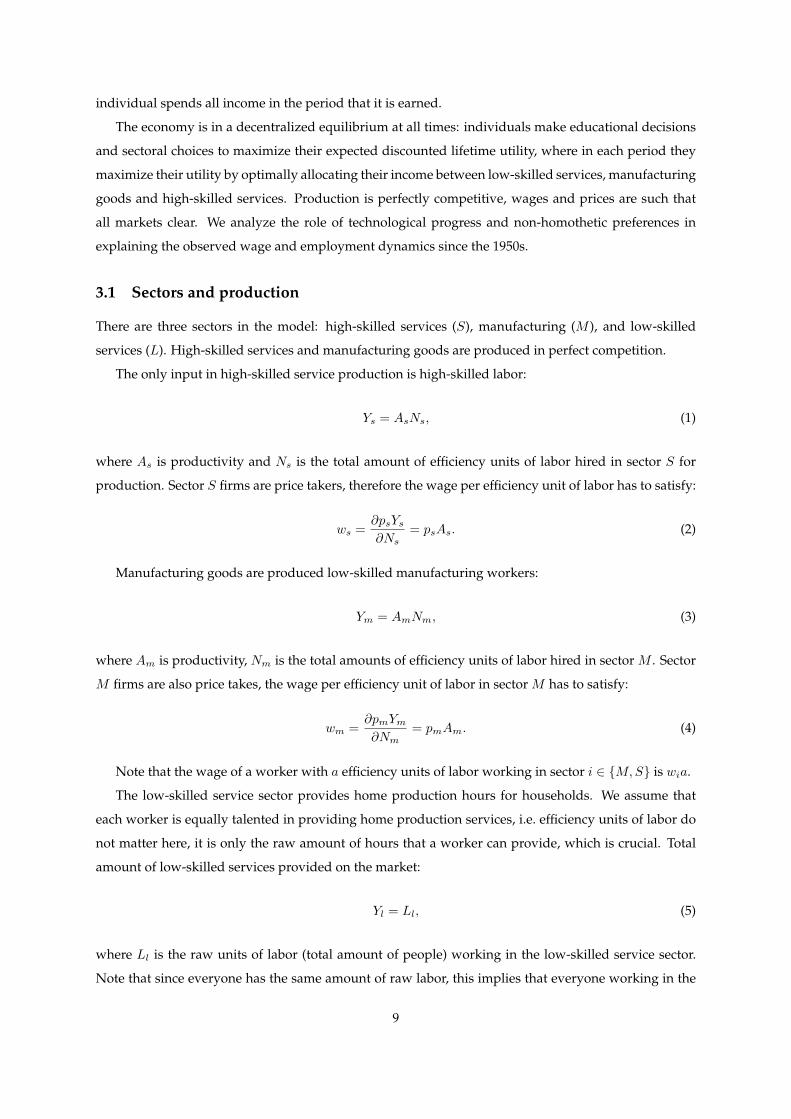
3.1 Sectors and production

There are three sectors in the model: high-skilled services (S), manufacturing (M ), and low-skilled

services (L). High-skilled services and manufacturing goods are produced in perfect competition.

The only input in high-skilled service production is high-skilled labor:

Ys = AsNs, (1)

where As is productivity and Ns is the total amount of efficiency units of labor hired in sector S for

production. Sector S firms are price takers, therefore the wage per efficiency unit of labor has to satisfy:

ws =∂psYs∂Ns

= psAs. (2)

Manufacturing goods are produced low-skilled manufacturing workers:

Ym = AmNm, (3)

where Am is productivity, Nm is the total amounts of efficiency units of labor hired in sector M . Sector

M firms are also price takes, the wage per efficiency unit of labor in sector M has to satisfy:

wm =∂pmYm∂Nm

= pmAm. (4)

Note that the wage of a worker with a efficiency units of labor working in sector i ∈ {M,S} is wia.

The low-skilled service sector provides home production hours for households. We assume that

each worker is equally talented in providing home production services, i.e. efficiency units of labor do

not matter here, it is only the raw amount of hours that a worker can provide, which is crucial. Total

amount of low-skilled services provided on the market:

Yl = Ll, (5)

where Ll is the raw units of labor (total amount of people) working in the low-skilled service sector.

Note that since everyone has the same amount of raw labor, this implies that everyone working in the

9

low-skilled service sector has the same earnings. The unit wage in this sector in equilibrium has to be

such that the total amount demanded of low-skilled services is equal to the amount supplied.

3.2 Labor supply and demand for goods

Time is infinite and discrete, indexed by t = 0, 1, 2... The economy is populated by a continuum of

individuals who live at most for T periods, but their survival probability declines as they get older, let

us denote these survival probabilities by λ ∈ RT , with λ(1) = 1.4 Every period a new generation of

measure 1/T is born. Individuals are heterogeneous in their innate ability (efficiency units of labor), a,

which is drawn at birth from a time invariant distribution f(a). These assumptions imply that both the

size of the population, and the distribution of abilities are constant over time.

Every agent has to decide at birth whether to acquire education or not. Agents choose their educa-

tion in order to maximize their expected discounted lifetime utility. Acquiring education grants access

to the high-skilled service sector (S), and the cost is twofold: there is a tuition fee, and a time cost. The

tuition fee is wsκ, which is proportional to the sectoral unit wage, ws.5 There is potentially a study time,

ψ, during which the worker does not earn any wages. We assume that the study time is less than one

period, i.e. ψ ∈ [0, 1]. We calibrate the length of one period in order for this assumption to be reasonable.

Those who acquire education have to work in the sector S in the remaining part of the first period.6

3.2.1 Sector of work

Each agent in every period of his life has to decide which sector to work in, taking as given his educa-

tion, his efficiency units of labor, and the sectoral unit wages. Since individuals cannot lend or borrow,

they choose their sector to maximize per period utility, which is equivalent to maximizing per period

income. Agents with education can work in sector S, M , or L. Agents without education can freely

choose between sector M and L.7

For workers without education it is optimal to work in sector M if

wm(t)a ≥ wl(t) ⇔ a ≥ wl(t)

wm(t)≡ alm(t). (6)

Therefore in period t among non-educated workers everyone with a < alm(t) works in sector L, and

everyone else works sector M .

Similarly educated workers prefer to work in sector S rather than L if

ws(t)a ≥ wl(t) ⇔ a ≥ wl(t)

ws(t)≡ als(t). (7)

4We introduce probabilistic survival in the OLG model to avoid the well known oscillations that arise with deterministic exit.See for example Abraham (2008).

5This assumption is made in order to have a steady state, and it is meant to represent the assumption that somebody workingin the same sector has to train the newly entering individual.

6This is assumed both for simplicity, and because we think of the education partly as training on the job.7In the steady state and the transition that we consider agents with education always optimally work in the sector S.

10

Therefore all educated workers with a ≥ als(t) work in sector S in period t.

It is not optimal for an educated worker to work in sector M if

ws(t)a ≥ wm(t)a ⇔ ws(t) ≥ wm(t).

Therefore in period t if wm(t) > ws(t) all the workers who are qualified to work in sector S work in

sector M instead. This also implies that there are no sector S workers available to train the potential

new entrants into sector S. Therefore in any such period there is no S production. This cannot be part

of an equilibrium unless the highest earner in period t does not demand any good S, and none of the

newborns wishes to get education.8

To summarize if ws(t) < wm(t), then the sector of work decision for educated and not educated

individuals is identical. If ws(t) ≥ wm(t), then all educated individuals with a ≥ als(t) work in sector

S, and those with a < als(t) work in sector L.

Since in their education decision individuals consider the lifetime utility from consumption, we

have to solve for their indirect utility given income.

3.2.2 Demand for consumption goods and low-skilled services

The individual maximizes the following utility in each period:

maxcm,cs,h

ln

θmc ε−1ε

m + θs(cs + γs)ε−1ε︸ ︷︷ ︸

C

εε−1

− φhν

ν

s.t. pmcm + pscs + wl(h− h︸ ︷︷ ︸=l

) ≤ m (λ0)

0 ≤ cs (µs), 0 ≤ cm (µm), 0 ≤ h (µl), h ≤ h ≡x

Ah(µh)

where m is the individual’s income in the given period, pm, ps are the prices of the manufacturing

and service goods, wl is the wage rate for low-skilled service workers. The total number of raw hours

needed for household work is h, which can vary over time. (Specifically we assume that Ahh = x,

where x is a constant. Therefore if Ah increases over time, then the necessary number of total home

production hours declines.) Doing the home production causes disutility to the individual, which is

increasing (φ > 0) in the number of hours spent on home production, and potentially convex (ν > 1).

The individual can hire a low-skilled service worker to do some or all of the home production.

The utility of the consumer is non-homothetic in manufacturing goods (cm) and high-skilled service

goods (cs). We assume that γs > 0, which is equivalent to assuming that cs is a luxury good, i.e. the

individual only demands a positive amount if it is sufficiently rich.

8We do not consider such steady states or transitions, as the support for efficiency units of labor is unbounded in the calibra-tion.

11

The following Corollary summarizes the solution to the consumer’s problem.

Corollary 1. The following cases can arise:

1. At the lowest income levels (m < m12 ≡ min{m12a,m12b}) the optimal choices are:

h = h (8)

cs = 0 (9)

cm =m

pm(10)

In this case µh > 0, µl = 0, µm = 0, µs > 0.

2. For higher income levels (m ∈ [m12,m23), where m23 ≡ min{m2a3,m2b3}),

A. if m ∈ [m12a,m2a3) and m12a < m12b the optimal choices are described by

cs = 0 (11)

h =

(wlpm

θmφ

) 1ν−1 (

θmcε−1ε

m + θsγε−1ε

s

)− 1ν−1

c− 1ε(ν−1)

m (12)

cm =m− wl(h− h)

pm(13)

In this case µh = 0, µl = 0, µm = 0, µs > 0.

B. if m ∈ [m12b,m2b3) and m12b < m12a, then the optimal choices are:

h = h (14)

cm =

(pmps

θsθm

)−ε(cs + γs) (15)

cs =m+ psγs

pm

(pmps

θsθm

)−ε+ ps

− γs (16)

In this case µh > 0, µl = 0, µm = 0, µs = 0.

3. For the highest income levels, if m > m23 the optimal choices are:

cs =

(pmps

θsθm

)εcm − γs (17)

h =

(wlpm

θmφ

) 1ν−1

(θm + θs

(pmps

θsθm

)ε−1)− 1ν−1

c− 1ν−1

m (18)

cm =m− pscs − wl(h− h)

pm(19)

In this case µh = 0, µl = 0, µm = 0, µs = 0.

12

The cutoff income levels are defined by the following equations: The cutoff m12a is the income level, where the

supply of h exactly equals h according to case 2a. We can find the cm for which h = h under case 2a. Then

m12a = pmcm(h = h). (20)

The cutoff m12b is the income level, where the demand for cs is exactly zero according to case 2b:

m12b = pm

(pmps

θsθm

)−εγs. (21)

The cutoff m2a3 is defined as the income level where the demand for cs is exactly zero under case 3 (therefore it

can only follow case 2a). Using that cs = 0 we get that cm =(pmps

θsθm

)−εγs. Using this value we can express

the optimal h under case 3, and can calculate the income level that way:

m2a3 = pm

(pmps

θsθm

)−εγs+wl

h− ( wlpm

θmφ

) 1ν−1

(θm + θs

(pmps

θsθm

)ε−1)− 1ν−1

((pmps

θsθm

)−εγs

)− 1ν−1

.

(22)

The cutoff m2b3 is the income level where the supply of h is exactly h under case 3 (therefore it can only follow

case 2b). Using that h = h we can express cm =(wlpm

θmφ

)(θm + θs

(pmps

θsθm

)ε−1)−1h−(ν−1)

, which therefore

gives the value of cs. The income that allows the purchase of that bundle is:

m2b3 =wlφh−(ν−1) − psγs. (23)

Proof. The Lagrangian of the problem is:

L(cm, cs, h) = lnCεε−1 − φh

ν

ν− λ(pmcm + pscs + wl(h− h︸ ︷︷ ︸

=l

)−m) + µscs + µmcm + µlh− µh(h− h)

The first order conditions are:

∂L∂cm

=1

Cθmc

− 1ε

m − λpm + µm = 0

∂L∂cs

=1

Cθs(cs + γs)

− 1ε − λps + µs = 0

∂L∂h

= −φhν−1 + λwl − µh + µl = 0

The solve the consumer’s problem we have to consider which constraints can be binding for which

income levels. First notice, that the non-negativity constraint on h never binds due to the specification

of the disutility from housework, if prices (pm, ps) and wages (wl) are positive and finite. Since the

disutility from housework goes to zero as h → 0, while the utility from consumption only goes to zero

as consumption goes to infinity, for finite income levels the household is always better off by increasing

c than reducing h to zero. The constraint on the non-negativity of cm can also never be binding, since the

13

marginal utility from consumption at cm = cs = 0 is infinity, while the marginal disutility of labor is a

positive, finite number. Therefore µm = 0 and µl = 0 always hold. By considering the other possibilities

the statement of the Corollary follows.

This implies that given parameters and prices the economy in a given period will be either in case

A or in case B. In both cases the poorest people (m < m12) only consume manufacturing goods, and

the highest earners (m > m23) consume everything. In case A middle income earners (m ∈ [m12,m23))

consume manufacturing goods and low-skilled services, whereas in case B they do all of their own

household work, but consume manufacturing goods and some high-skilled services. Each consumer

can be considered poor, middle income, or rich depending on which sets of goods and services they

consume optimally. Given sectoral wage rates, we can determine the demand coming from each type

of worker.

All low-skilled service workers consume the same consumption bundle, as they all receive the same

income, wl. Depending on the position of wl relative to m12 and m23, they are all either poor, middle

income, or rich consumers.

Since the manufacturing sector workers’ earnings depend on their ability, awm, those who have a

different ability have a different consumption bundle, and potentially they are different types of con-

sumers. Those with a < m12/wm are considered poor9, those with a ∈ [m12/wm,m23/wm) are middle

income, and those with a > m23/wm are rich consumers10, they consumer everything.

The high-skilled service workers can also be categorized into poor, middle income or rich con-

sumers, where the cutoff ability for belonging to the above categories are respectively, m12/ws and

m23/ws.11

Given optimal sector of work choice and education decisions, the total demand for each of the ser-

vices and the manufacturing goods can be calculated by aggregating the demand coming from each

type of worker from each cohort who is alive in the given period.

To determine the optimal educational decision, we need to calculate the expected discounted life-

time utility from each choice, for which we need to calculate the individual’s per period utility. Based

on Corollary 1, for a given vector of prices p ≡ [pm, ps, wl], the indirect utility function of a consumer

with income m can be easily constructed. Let V U(m;p) denote this per period indirect utility function.

3.2.3 Choice of education

Given the possibility of workers to choose sectors and the above defined indirect utility function, the

expected discounted lifetime utility of a worker with education S, efficiency units of labor a, born at

9There can only be manufacturing workers like this is m12/wm > alm, otherwise all manufacturing workers are at leastconsidered middle income consumers.

10There can only be manufacturing workers like this if at least some past education cutoff as < m23/wm.11It is again possible that there are no poor, or middle income high-skilled service workers, i.e. there are no high-skilled

workers with ability below m12/ws or m23/ws.

14

time t can be written as:

Vs(a, t) =V U((1− ψ)ws(t)a− ws(t)κ;p(t))

+

T−t∑i=t+1

βi−tλ(i− t+ 1)V U(max{ws(i)a,wm(i)a,wl(i)};p(i)).

Expected discounted lifetime utility of a worker without education, with efficiency units of labor a,

born at time t is:

Vn(a, t) =

T−t∑i=t

βi−tλ(i− t+ 1)V U(max{wm(i)a,wl(i)};p(i)).

Note that in both cases (N , S) the expected present value of lifetime utility is increasing in ability,

a, of the individual. This implies that between any two options, the optimal decision rule can be sum-

marized by a set of cut-off ability levels, which determine ranges of abilities, a, where one decision is

optimal, while for other ability levels, the other decision is optimal.

Lemma 1. The optimal educational choice in period t can be described by a unique cutoff ability level as(t),

defined as the solution of:

Vs(as(t), t) = Vn(as(t), t). (24)

For individuals born in period t with a < as(t) it is optimal to remain low-skilled, while for all individuals born

in period t with a ≥ as(t) it is optimal to acquire education.

Proof. It is optimal to acquire education if the following difference is positive:

Vs(a, t)− Vn(a, t) = V U((1− ψ)ws(t)a− ws(t)κ;p(t))− V U(max{wm(t)a,wl(t)};p(t))︸ ︷︷ ︸first period gain or loss

+

T−t∑i=t+1

βi−tλ(i− t+ 1) (V U(max{ws(i)a,wm(i)a,wl(i)},p(i))− V U(max{wm(i)a,wl(i)},p(i)))︸ ︷︷ ︸≥0 and increasing in a

.

In the Appendix we show that this function is continuous, negative for a = 0, and crosses zero only

once.

Deriving the labor supply in period s of a cohort born in period 0 < t ≤ s is straightforward given

Lemma 1, and given the unit wages in each sector in period s.

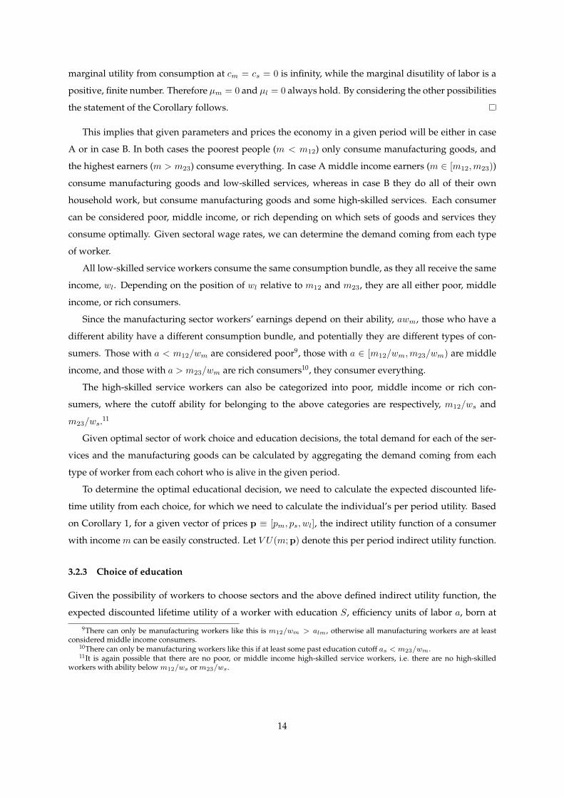
Corollary 2. The cohort born in period t > 0 supplies labor to each sector in period s in the following way.

15

1. If the period s unit wages satisfy wm(s) ≤ ws(s), and as(t) ≤ alm(s), then

Ll(t, s) =λ(s− t+ 1)

T

∫ max{als(s),as(t)}

0

f(a)da (25)

Nm(t, s) = 0 (26)

Ns(t, s) =λ(s− t+ 1)

T

∫ ∞max{als(s),as(t)}

af(a)da (27)

2. If the period s unit wages satisfy wm(s) ≤ ws(s), and alm(s) < as(t), then

Ll(t, s) =λ(s− t+ 1)

T

∫ alm(s)

0

f(a)da (28)

Nm(t, s) =λ(s− t+ 1)

T

∫ as(t)

alm(s)

af(a)da (29)

Ns(t, s) =λ(s− t+ 1)

T

∫ ∞as(t)

af(a)da (30)

3. If wm(s) > ws(s), then

Ll(t, s) =λ(s− t+ 1)

T

∫ alm(s)

0

f(a)da (31)

Nm(t, s) =λ(s− t+ 1)

T

∫ ∞alm(s)

af(a)da (32)

Ns(t, s) = 0 (33)

Proof. It is easy to see that we have covered each possible configuration of cutoffs. See Appendix for

details.

Corollary 3. The effective labor supply in period s of workers born in period s:

Ll(s, s) =1

T

(∫ min{as(s),alm(s)}

0

f(a)da

); (34)

Nm(s, s) =1

T

∫ as(s)

min{as(s),alm(s)}af(a)da; (35)

Ns(s, s) =1

T(1− ψs)

∫ ∞as(s)

af(a)da− 1

Tκ

∫ ∞as(s)

f(a)da. (36)

Proof. Using the fact that education takes time, those born in period s, who get educated only work in a

fraction (1−ψ) of period s. On top of this, those who acquire education require training, in the amount κ

for each individual. This amount of labor is used for their training, rather than for production, therefore

they reduce the effective labor supply by this amount per person.

Assumption 1. We assume that the economy starts in period 0, with T cohorts, one from each generation, and

each generation made education decisions according to 0 < as(0) <∞.

16

Note that this assumption is equivalent to assuming that the economy from the start of time (t =

−∞) has been in a steady state where the optimal educational decision is given by cutoffs 0 < as(0) <

∞, and whatever change (if any) happened in period 1 was unanticipated by all agents born until period

0.

Corollary 4. Assume that the period s unit wages satisfy wm(s) ≤ ws(s). The cohort born in period t = 0

supplies labor to each sector in period s ≤ T − 1 in a similar way as in Corollary 2 except the multiplier is∑s+1i=1 λ(i)/T instead of λ(s+ 1)/T which would be indicated by applying Corollary 2 to t = 0.

Given the labor supplies by each cohort in Corollaries 2 and 3 the total effective labor supply in

period s is given by:

Ll(s) =

s∑j=s−T+1

Ll(s− j, s) (37)

Nm(s) =

s∑j=s−T+1

Nm(s− j, s) (38)

Ns(s) =

s∑j=s−T+1

Ns(s− j, s) (39)

4 Competitive Equilibrium

A competitive equilibrium is a sequence of cutoff education abilities {as(t)}∞t=1, labor supply abilities

{alm(t), als(t)}∞t=1, wages {wl(t), wm(t), ws(t)}∞t=1, prices {pm(t), ps(t)}∞t=1, given the path of productiv-

ities {Ah(t), Am(t), As(t)}∞t=0 and initial education decisions as(0) which satisfy:

1. as(t) is the solution to equation (24);

2. alm(t), als(t) are defined as in (6), and (7);

3. the unit wage rates are such that the market for L, M and S labor clears;

4. pm and ps are such that the market for M goods and S goods clears.

The economy is always in a competitive equilibrium, where newborns choose their education opti-

mally, and older cohorts choose their sector of work optimally. Firms maximize their profits. Markets

clear.

For any initial condition, there is a unique stationary competitive equilibrium, which features con-

stant education and sector-of-work decisions. In a steady state the following holds for the education

and sector-of-work decisions:

alm =wlwm

;

17

while as satisfies

V U(ws((1− ψ)as − κ);p)− V U(wmas;p) + (V U(wsas,p)− V U(wmas,p))

T∑i=2

βiλ(i) = 0.

In the steady state the effective and raw labor supplies are given by:

Ll =

∫ alm

0

1dF (a);

Nm =

∫ as

alm

adF (a); Lm =

∫ as

alm

1dF (a);

Ns =

(∑Ti=2 λ(i) + (1− ψ)

)T

∫ ∞as

adF (a)− 1

Tk

∫ ∞as

1dF (a); Ls =

∫ ∞as

1dF (a).

Therefore across different steady states it holds that Ll increases with wl/wm, andNs(Ls) increases with

ws/wm. This is similar to some kind of polarization: if the relative unit wages increase at the top and at

the bottom, then the raw labor supplies move the same way. However, in reality we do not observe the

relative unit wages, but we observe the relative average wages.

5 Quantitative results (Incomplete)

In this section we quantitatively assess the contribution of structural transformation to the polarization

of employment and wages across industries. To do this we consider the economy to be on a full foresight

transition to the steady state. The model economy starts in 1950, and all workers/consumers are aware

that there will be 120 years of unequal productivity growth. We calibrate the first period of the transition

to match some 1950 data moments. We first describe the data targets and the calibration strategy, and

then discuss the quantitative importance of our mechanism.

5.1 Data targets

We calibrate our model to replicate six key moments of the US economy in 1950. These moments are

the relative average industry wages, the industry employment shares and the sectoral value added

shares. Data for the average industry wages and the industry employment shares come from the 1950

US Census data. Each employed individual is categorized as a high-skilled service, manufacturing or

low-skilled service worker, based on their industry code (ind1990). Employment shares are calculated

as share of hours worked. We regress log hourly wages on worker age and its square, a female dummy, a

born-abroad dummy and a non-white dummy. The relative industry wages are calculated as the ratio of

the average of the exponential of the residual wages across industries. For sectoral value added shares

we rely on the National Income and Product Accounts (NIPA), but adjust them for intermediaries using

the input-output tables published by the Bureau of Economic Analysis (BEA), similar to Herrendorf,

Rogerson, and Valentinyi (2013).

18

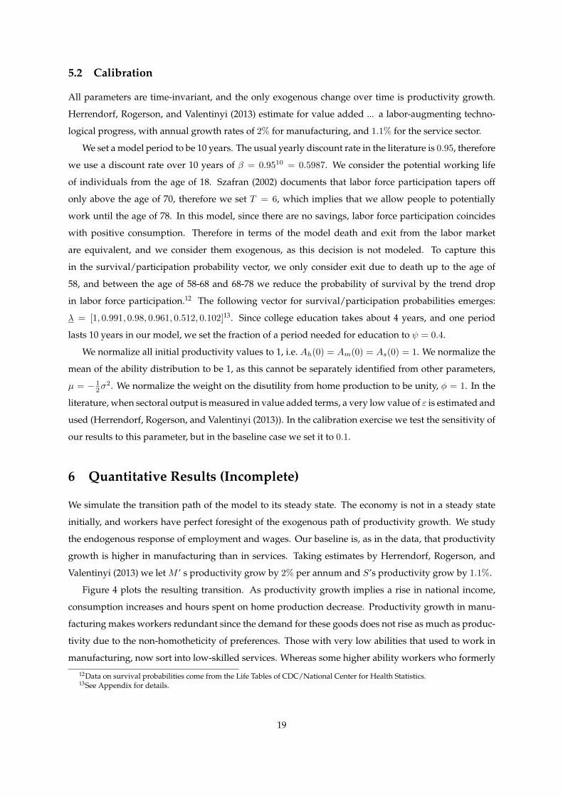
5.2 Calibration

All parameters are time-invariant, and the only exogenous change over time is productivity growth.

Herrendorf, Rogerson, and Valentinyi (2013) estimate for value added ... a labor-augmenting techno-

logical progress, with annual growth rates of 2% for manufacturing, and 1.1% for the service sector.

We set a model period to be 10 years. The usual yearly discount rate in the literature is 0.95, therefore

we use a discount rate over 10 years of β = 0.9510 = 0.5987. We consider the potential working life

of individuals from the age of 18. Szafran (2002) documents that labor force participation tapers off

only above the age of 70, therefore we set T = 6, which implies that we allow people to potentially

work until the age of 78. In this model, since there are no savings, labor force participation coincides

with positive consumption. Therefore in terms of the model death and exit from the labor market

are equivalent, and we consider them exogenous, as this decision is not modeled. To capture this

in the survival/participation probability vector, we only consider exit due to death up to the age of

58, and between the age of 58-68 and 68-78 we reduce the probability of survival by the trend drop

in labor force participation.12 The following vector for survival/participation probabilities emerges:

λ = [1, 0.991, 0.98, 0.961, 0.512, 0.102]13. Since college education takes about 4 years, and one period

lasts 10 years in our model, we set the fraction of a period needed for education to ψ = 0.4.

We normalize all initial productivity values to 1, i.e. Ah(0) = Am(0) = As(0) = 1. We normalize the

mean of the ability distribution to be 1, as this cannot be separately identified from other parameters,

µ = − 12σ

2. We normalize the weight on the disutility from home production to be unity, φ = 1. In the

literature, when sectoral output is measured in value added terms, a very low value of ε is estimated and

used (Herrendorf, Rogerson, and Valentinyi (2013)). In the calibration exercise we test the sensitivity of

our results to this parameter, but in the baseline case we set it to 0.1.

6 Quantitative Results (Incomplete)

We simulate the transition path of the model to its steady state. The economy is not in a steady state

initially, and workers have perfect foresight of the exogenous path of productivity growth. We study

the endogenous response of employment and wages. Our baseline is, as in the data, that productivity

growth is higher in manufacturing than in services. Taking estimates by Herrendorf, Rogerson, and

Valentinyi (2013) we let M ’ s productivity grow by 2% per annum and S’s productivity grow by 1.1%.

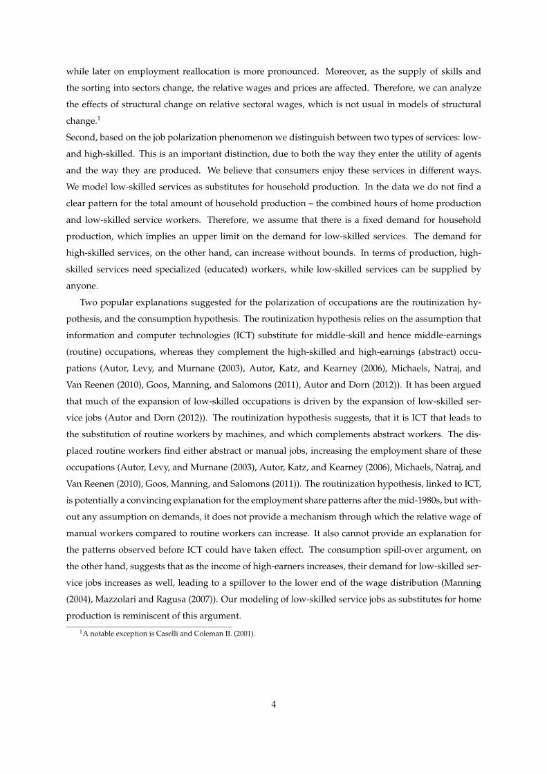
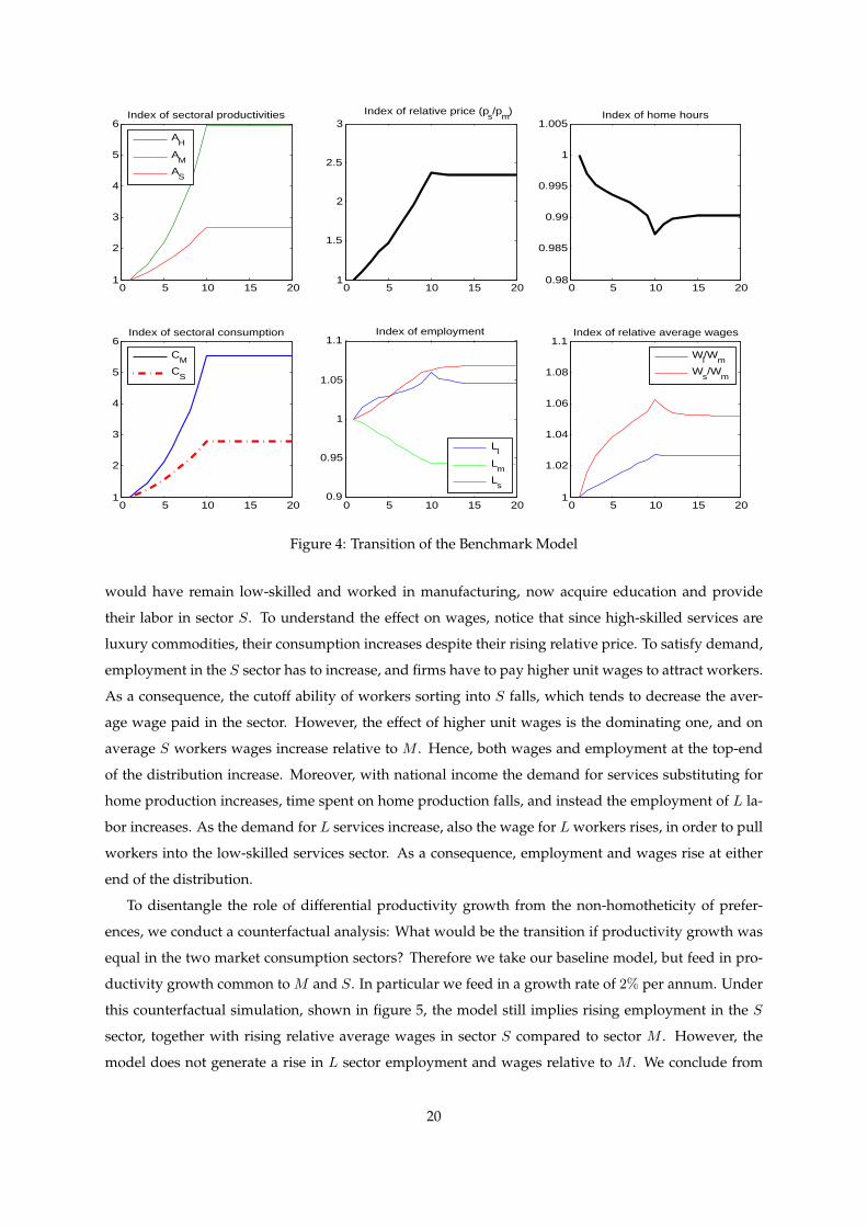
Figure 4 plots the resulting transition. As productivity growth implies a rise in national income,

consumption increases and hours spent on home production decrease. Productivity growth in manu-

facturing makes workers redundant since the demand for these goods does not rise as much as produc-

tivity due to the non-homotheticity of preferences. Those with very low abilities that used to work in

manufacturing, now sort into low-skilled services. Whereas some higher ability workers who formerly

12Data on survival probabilities come from the Life Tables of CDC/National Center for Health Statistics.13See Appendix for details.

19

0 5 10 15 201

2

3

4

5

6Index of sectoral productivities

A

H

AM

AS

0 5 10 15 201

1.5

2

2.5

3Index of relative price (p

s/p

m)

0 5 10 15 200.98

0.985

0.99

0.995

1

1.005Index of home hours

0 5 10 15 201

2

3

4

5

6Index of sectoral consumption

C

M

CS

0 5 10 15 200.9

0.95

1

1.05

1.1Index of employment

Ll

Lm

Ls

0 5 10 15 201

1.02

1.04

1.06

1.08

1.1Index of relative average wages

W

l/W

m

Ws/W

m

Figure 4: Transition of the Benchmark Model

would have remain low-skilled and worked in manufacturing, now acquire education and provide

their labor in sector S. To understand the effect on wages, notice that since high-skilled services are

luxury commodities, their consumption increases despite their rising relative price. To satisfy demand,

employment in the S sector has to increase, and firms have to pay higher unit wages to attract workers.

As a consequence, the cutoff ability of workers sorting into S falls, which tends to decrease the aver-

age wage paid in the sector. However, the effect of higher unit wages is the dominating one, and on

average S workers wages increase relative to M . Hence, both wages and employment at the top-end

of the distribution increase. Moreover, with national income the demand for services substituting for

home production increases, time spent on home production falls, and instead the employment of L la-

bor increases. As the demand for L services increase, also the wage for L workers rises, in order to pull

workers into the low-skilled services sector. As a consequence, employment and wages rise at either

end of the distribution.

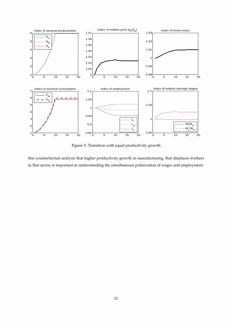
To disentangle the role of differential productivity growth from the non-homotheticity of prefer-

ences, we conduct a counterfactual analysis: What would be the transition if productivity growth was

equal in the two market consumption sectors? Therefore we take our baseline model, but feed in pro-

ductivity growth common to M and S. In particular we feed in a growth rate of 2% per annum. Under

this counterfactual simulation, shown in figure 5, the model still implies rising employment in the S

sector, together with rising relative average wages in sector S compared to sector M . However, the

model does not generate a rise in L sector employment and wages relative to M . We conclude from

20

0 5 10 15 201

2

3

4

5

6Index of sectoral productivities

A

H

AM

AS

0 5 10 15 201

1.01

1.02

1.03

1.04

1.05

1.06

1.07Index of relative price (p

s/p

m)

0 5 10 15 200.98

0.99

1

1.01

1.02

1.03Index of home hours

0 5 10 15 201

2

3

4

5

6

7Index of sectoral consumption

C

M

CS

0 5 10 15 200.85

0.9

0.95

1

1.05

1.1Index of employment

Ll

Lm

Ls

0 5 10 15 200.95

1

1.05

1.1Index of relative average wages

Wl/W

m

Ws/W

m

Figure 5: Transition with equal productivity growth

this counterfactual analysis that higher productivity growth in manufacturing, that displaces workers

in that sector, is important in understanding the simultaneous polarization of wages and employment.

21

References

ABRAHAM, A. (2008): “Earnings inequality and skill-biased technological change with endogenous

choice of education,” Journal of the European Economic Association, 6(2-3), 695–704.

ACEMOGLU, D., AND D. AUTOR (2011): “Chapter 12 - Skills, Tasks and Technologies: Implications for

Employment and Earnings,” vol. 4, Part B of Handbook of Labor Economics, pp. 1043 – 1171. Elsevier.

ACEMOGLU, D., AND V. GUERRIERI (2008): “Capital Deepening and Nonbalanced Economic Growth,”

Journal of Political Economy, 116(3), pp. 467–498.

AUTOR, D. H., AND D. DORN (2012): “The Growth of Low Skill Service Jobs and the Polarization of the

U.S. Labor Market,” The American Economic Review.

AUTOR, D. H., L. F. KATZ, AND M. S. KEARNEY (2006): “The Polarization of the U.S. Labor Market,”

The American Economic Review, 96(2), pp. 189–194.

AUTOR, D. H., F. LEVY, AND R. J. MURNANE (2003): “The Skill Content of Recent Technological

Change: An Empirical Exploration,” The Quarterly Journal of Economics, 118(4), pp. 1279–1333.

BOPPART, T. (2011): “Structural Change and the Kaldor Facts in a Growth Model with Relative Price

Effects and Non-Gorman Preferences,” Working paper no. 2, University of Zurich Department of

Economics.

BUERA, F. J., AND J. P. KABOSKI (2009): “CAN TRADITIONAL THEORIES OF STRUCTURAL

CHANGE FIT THE DATA?,” Journal of the European Economic Association, 7(2-3), 469–477.

(2012a): “The Rise of the Service Economy,” American Economic Review, 102(6), 2540–69.

(2012b): “Scale and the origins of structural change,” Journal of Economic Theory, 147(2), 684 –

712, ¡ce:title¿Issue in honor of David Cass¡/ce:title¿.

CASELLI, F., AND W. J. COLEMAN II. (2001): “The U.S. Structural Transformation and Regional Con-

vergence: A Reinterpretation,” Journal of Political Economy, 109(3), pp. 584–616.

GOOS, M., AND A. MANNING (2007): “Lousy and Lovely Jobs: The Rising Polarization of Work in

Britain,” The Review of Economics and Statistics, 89(1), 118–133.

GOOS, M., A. MANNING, AND A. SALOMONS (2009): “Job Polarization in Europe,” The American Eco-

nomic Review, 99(2), pp. 58–63.

(2011): “Explaining job polarization: the roles of technology, offshoring and institutions,” Open

Access publications from Katholieke Universiteit Leuven urn:hdl:123456789/331184, Katholieke Uni-

versiteit Leuven.

22

HERRENDORF, B., R. ROGERSON, AND K. VALENTINYI (2013): “Two Perspectives on Preferences and

Structural Transformation,” American Economic Review, 103(7), 2752–89.

KONGSAMUT, P., S. REBELO, AND D. XIE (2001): “Beyond Balanced Growth,” The Review of Economic

Studies, 68(4), pp. 869–882.

KUZNETS, S. (1957): “Quantitative Aspects of the Economic Growth of Nations: II. Industrial Distri-

bution of National Product and Labor Force,” Economic Development and Cultural Change, 5(4), pp.

1–111.

MADDISON, A. (1980): “Economic Growth and Structural Change in the Advanced Countries,” in West-

ern Economies in Transition: Structural Change and Adjustment Policies in Industrial Countries, ed. by

I. Leveson, and J. W. Wheeler, pp. 41–65. London: Croom Helm.

MANNING, A. (2004): “We Can Work It Out: The Impact of Technological Change on the Demand for

Low-Skill Workers,” Scottish Journal of Political Economy, 51(5), 581–608.

MAZZOLARI, F., AND G. RAGUSA (2007): “Spillovers from high-skill consumption to low-skill labor

markets,” The Review of Economics and Statistics, (0).

MEYER, P. B., AND A. M. OSBORNE (2005): “Proposed Category System for 1960-2000 Census Occupa-

tions,” Working Papers 383, U.S. Bureau of Labor Statistics.

MICHAELS, G., A. NATRAJ, AND J. VAN REENEN (2010): “Has ICT Polarized Skill Demand? Evidence

from Eleven Countries over 25 years,” Working Paper 16138, National Bureau of Economic Research.

NGAI, L. R., AND C. A. PISSARIDES (2007): “Structural Change in a Multisector Model of Growth,” The

American Economic Review, 97(1), pp. 429–443.

(2008): “Trends in hours and economic growth,” Review of Economic Dynamics, 11(2), 239 – 256.

SZAFRAN, R. F. (2002): “Age-adjusted labor force participation rates, 1960-2045.,” Monthly Labor Review,

125(9), 25.

23

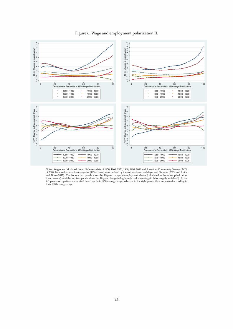
Figure 6: Wage and employment polarization II.-.2

0.2

.4.6

.81

1.2

1.4

10-Y

r Cha

nge

in ln

(real

wag

e)

0 20 40 60 80 100Occupation's Percentile in 1950 Wage Distribution

1950 - 1960 1960 - 19701970 - 1980 1980 - 19901990 - 2000 2000 - 2008

-.20

.2.4

.6.8

11.

21.

41.

610

-Yr C

hang

e in

ln(re

al w

age)

0 20 40 60 80 100Occupation's Percentile in 1980 Wage Distribution

1950 - 1960 1960 - 19701970 - 1980 1980 - 19901990 - 2000 2000 - 2008

-.4-.3

-.2-.1

0.1

.2.3

.410

-Yr C

hang

e in

Em

ploy

men

t Sha

re

0 20 40 60 80 100Occupation's Percentile in 1950 Wage Distribution

1950 - 1960 1960 - 19701970 - 1980 1980 - 19901990 - 2000 2000 - 2008

-.4-.3

-.2-.1

0.1

.2.3

.410

-Yr C

hang

e in

Em

ploy

men

t Sha

re

0 20 40 60 80 100Occupation's Percentile in 1980 Wage Distribution

1950 - 1960 1960 - 19701970 - 1980 1980 - 19901990 - 2000 2000 - 2008

Notes: Wages are calculated from US Census data of 1950, 1960, 1970, 1980, 1990, 2000 and American Community Survey (ACS)of 2008. Balanced occupation categories (185 of them) were defined by the authors based on Meyer and Osborne (2005) and Autorand Dorn (2012). The bottom two panels show the 10-year change in employment shares (calculated as hours supplied ratherthan persons), and the top two panels show the 10-year change in log hourly real wages (again labor supply weighted). In theleft panels occupations are ranked based on their 1950 average wage, whereas in the right panels they are ranked according totheir 1980 average wage.

24