Job matching across occupational labour markets

Job matching across occupational labourmarkets

By Michael Stops

Institute for Employment Research/Institut fur Arbeitsmarkt- und

Berufsforschung (IAB), Weddigenstraße 20-22, 90479 Nuremberg, Germany;

e-mail: [email protected]

The article refers to job matching processes in occupational labour markets in terms of

jobs that share extensive commonalities in their required qualifications and tasks. To

date, all studies in this field have been based on the assumption that matching processes

only transpire within distinct occupational labour markets and that no occupational

changes occur. I present theoretical and empirical arguments that undermine the

validity of this assumption. I construct an ‘occupational topology’ based on information

about the ways occupational groups may be seen as alternatives in searches for jobs or

workers. I then use different empirical models that consider cross-sectional dependency

to test the hypothesis that job search and matching occur across occupational labour

markets. The results support my hypothesis. The findings suggest that an augmented

empirical model should be used that considers job and worker searches across occupa-

tional labour markets in estimating job matching elasticities.

JEL classification: C21, C23, J44, J64.

1. IntroductionThe determinants of matching labour demand and labour supply to create new jobs

are of continual interest for both labour market researchers and politicians. Partly

because it is difficult to observe the individual search processes that underlie this

type of matching on the micro level, studies in this field typically refer to the

analytical results obtained using macroeconomic matching functions that model

the empirical dependency of the number of new hires on the number of job seekers

and vacancies in a particular context of interest; for an overview of the foregoing,

compare the surveys of Petrongolo and Pissarides (2001), Rogerson et al. (2005),

and Yashiv (2007). These studies help elucidate the efficiency of matching processes

in both aggregated and partial labour markets. Therefore, studies examined

particular sectors (Broersma and van Ours, 1999), regions (Anderson and

Burgess, 2000; Kangasharju et al., 2005), or occupational groups, which are

classes of jobs that share extensive commonalities in their qualification require-

ments and tasks (Entorf, 1994; Fahr and Sunde, 2004; Mora and Santacruz, 2007;

Stops and Mazzoni, 2010). The central assumption of most studies in this field is

! Oxford University Press 2014All rights reserved

Oxford Economic Papers 66 (2014), 940–958 940doi:10.1093/oep/gpu018

at Nova Southeastern U

niversity on Novem

ber 28, 2014http://oep.oxfordjournals.org/

Dow

nloaded from

http://oep.oxfordjournals.org/

that partial labour markets are completely separated from each other; in other

words, there are no flows of job seekers from one partial labour market to

another partial labour market, and no correlations exist between different labour

markets with respect to newly created jobs or numbers of job vacancies. This central

assumption is not presumed by studies of regional labour markets (e.g., Burda and

Profit, 1996; Fahr and Sunde, 2006; Dauth et al., 2010; Lottmann, 2012) that

consider the penetrability of partial labour markets. However, to date, no study

of occupational labour markets has considered the dependencies between these

partial labour markets. In investigations by Entorf (1994), Fahr and Sunde

(2004), Mora and Santacruz (2007), and Stops and Mazzoni (2010), the number

of new jobs in a given occupational group is explained by the number of

unemployed workers and vacancies in same occupational group.

In this article, I use both theoretical and empirical arguments to demonstrate

that the assumption of separate occupational labour markets is not appropriate.

I test my hypotheses using pooled ordinary least squares, fixed effects, and pooled

mean-group models that include cross-sectional dependency lags of regressors.

Therefore, the estimators take into account interactions between cross-sectional

units. To achieve this purpose, I construct an empirically based ‘occupational

topology’—as analogon to the spatial order of regions—in terms of a matrix that

contains information about occupations that either are assumed to be substitutes

for recruitment and employment or are not assumed to be substitutes following the

considerations by Gathmann and Schonberg (2010) and Matthes et al. (2008).

I discuss empirically and theoretically if job matching models that consider job

searchers and vacancies in other occupational substitutes as explaining variables for

new matches should be preferred. If that applies, these models adjust and

complement the well-known (direct) matching elasticities of vacancies and job

searchers in the occupational labour markets of interest with (indirect) matching

elasticities of vacancies and job searchers in occupational groups that are

considered to be substitutes to one another.

In the following section, I describe the motivation and theoretical framework of

my estimation approach to the matching function. In Section 3, I present the data

used in this study, and the empirical estimates are subsequently provided in Section

4. Section 5 summarizes the main results of the investigation.

2. Motivation and theoretical frameworkThe standard model of the matching function assumes the existence of a homoge-

neous pool of unemployed workers and a homogeneous pool of vacancies. The

search activities of both sides of the market can be described as a matching

technology. The processes underlying this matching procedure are not explicitly

modelled;1 instead, the matching process can be regarded as a black box

..........................................................................................................................................................................1 Examples of these processes include job and worker search decisions, job searches, and negotiations of

wages.

m. stops 941


niversity on Novem


Dow

nloaded from


(Petrongolo and Pissarides, 2001). The variables U, V, and M may be used to

represent the numbers of unemployed workers, vacancies, and new hires

(matches), respectively. The matching function f(U,V) is frequently specified

using a Cobb-Douglas functional form:

M ¼ AU�U V�V ð1Þ

where A describes the ‘augmented’ matching productivity (e.g., Fahr and Sunde,

2004). The coefficients �U and �V represent the matching elasticities of

unemployed and vacancies, respectively. In accordance with standard matching

theory, both elasticities are positive. Furthermore, the theoretical model assumes

constant returns to scale, which implies that �U þ �V ¼ 1 with �U ,�V > 0.

In the following, the assumption of homogeneous pools of vacancies and

unemployed workers will be relaxed. It is reasonable to assume that occupation-

specific differences exist with respect to the matching processes due to differences in

job requirements, apprenticeships, and other factors (for empirical evidence, see

Fahr and Sunde, 2004; Stops and Mazzoni, 2010). In Germany, in particular, oc-

cupations are more suitable units than regions or economic sectors for analyses of

matching processes (compare with Fahr and Sunde, 2004), because occupations

include specific qualification requirements, tasks, and other characteristics.

Furthermore, individuals in Germany acquire occupation-specific knowledge

over the courses of their careers. Typically firms with vacancies attempt to hire

workers with certain qualifications, whereas job searchers seek jobs in certain oc-

cupations. The aforementioned studies (Fahr and Sunde, 2004; Stops and Mazzoni,

2010) assume that the number of new jobs in an occupational group does not

depend on the number of unemployed workers and vacancies in other occupational

groups. Fahr and Sunde (2004) propose the existence of partial occupational labour

markets that are aggregates of specific occupational groups. These labour markets

should be separated from each other; no flows of workers between different occu-

pational labour markets should occur, and no correlations should exist between

different labour markets with respect to newly created jobs or numbers of job

vacancies, but this may be the case within these markets. Both Fahr and Sunde

(2004) and Stops and Mazzoni (2010) use data on occupational groups that are

assigned to each occupational labour market to estimate matching elasticities for

these markets. However, these researchers do not explicitly engage in either

empirical or theoretical considerations of the flows or correlations between

different occupations. Therefore, they assume that partial labour markets in

terms of occupational groups are completely separate.

However, occupational labour markets could certainly interact with each other

with respect to the matching process. One argument for the existence of these

interactions is that both unemployed and employed persons change their occupa-

tions during their employment careers (Fitzenberger and Spitz, 2004; Seibert, 2007;

Kambourov and Manovskii, 2009; Gathmann and Schonberg, 2010; Schmillen and

Moller, 2012). An observation of the flows of individuals into employment between

942 job matching across occupations


niversity on Novem


Dow

nloaded from


1982 and 2007 reveals that the shares of these flows that involve occupational

changes is rather large in certain industries. In particular, these shares range

from 16% (the occupational changes of former foresters and huntsmen) to 75%

(the occupational changes of polymer processors).2 These empirical examples show

clearly that assumption of no mobility between occupational labour markets is even

too strict for Germany. Furthermore, this should also apply a fortiori to countries

such as the UK and the USA, both of which have labour markets that are less

structured by well-defined job titles.

From a theoretical point of view, the incorporation of flows between occupa-

tional labour markets causes analyses of the matching process to become consid-

erably more complex: job searchers must decide on their search strategy with

respect to their optimal numbers of job interviews in several different occupational

labour markets.

In the following discussion, I use a theoretical matching model that offers deeper

insights into the implications for the matching elasticities for unemployed workers

and vacancies that derive from the fact that job and worker searches occur not only

within occupational labour markets but also across these markets. Although the

structure of this model is based on a paper by Burda and Profit (1996), the inter-

pretation of the model has been widely modified. According to the model and

under certain assumptions,3 the optimal search intensity N�ij of an individual

with (former) occupation i in a job search in the new or same occupation j

depends negatively on the costs of the job search c + auDij with a fixed

component c and a component associated with searching in other occupational

groups that consists of a cost rate au and a dissimilarity measure Dij for occupations

i and j, positively on returns for a successful job search in terms of wages adjusted

by the interest rate w/r, and negatively on the probability of obtaining a job after

completing a job application pj in the case in which the expected gain from job

search highly exceeds the costs; in the opposite case N�ij would be zero:

N�ij ¼1pj

ln�ðw=rÞpj

cþauDij

�for w

r pj5ðc þ auDijÞ

0 for wr pj < ðc þ auDijÞ

8<: ð2Þ

The negative relationship between optimal job search intensity and the probabil-

ity of obtaining a job after applying arises from the assumption that the search costs

are linear and should be significantly smaller than the expected revenues from the

job search; thus, ðw=rÞpj�c þ auDij.4

..........................................................................................................................................................................2 See the online Appendix A.1 for more detailed information.3 The formal considerations for this model are presented in Appendix A.2.4 This finding contradicts the standard assumption of the discouraged worker hypothesis (Pissarides,

2000). According to this hypothesis, workers increase their job search intensity when the probability of

obtaining a job increases but give up their search when the expected revenues from the search are

relatively low. The hypothesis is derived from a model that assumes that search costs increase exponen-

tially with job search intensity. Under the conditions of this model, optimal job search intensity depends

positively on the job finding probability. The framework of the model is rather controversial; in

m. stops 943


niversity on Novem


Dow

nloaded from

http://oep.oxfordjournals.org/lookup/suppl/doi:10.1093/oep/gpu018/-/DC1



In their analysis of regional labour markets, Burda and Profit (1996)

complement fixed search costs c from standard search models with the variable

element auDij, which depends positively on the distance Dij between the region i in

which a job searcher is located and the region j in which this individual is searching

for a job. With respect to permeability, occupational labour markets may resemble

regional labour markets.

In particular, workers and vacancies are typically associated with particular oc-

cupational groups. Nevertheless, workers and firms often do not limit their search

to a single occupational labour market. With respect to regional labour markets,

various metrics—such as geographic distances or commuting flows—should

represent the strength of the interdependencies (and causal relationships)

between economic activities in different regions. In many instances, the topology

of the regions of interest provides a good indicator of the relationships that must be

analysed. In occupational labour markets, the resulting ‘topology’ becomes more

complex because there are no physical restrictions on the numbers of borders and

neighbours of particular occupational groups. Thus, metrics are required that

represent similarities amongst occupational groups with respect to their property

as alternatives for both job searchers and firms that are seeking workers.

In the following analyses, I differentiate only between the case of two or more

occupations that are similar because they are plausible alternatives in the job search

and matching process and the opposite case that consists of dissimilar occupations.

Therefore, in the model, I assume that the variable portion of search costs might be

zero if a job searcher is searching in his former occupational labour market (Dij = 0),

positive but moderate for a job search in similar occupational markets

(Dij ¼ d; 0 < d�1), or prohibitively high for a job search in dissimilar occupa-

tional labour markets (Dij !1). Thus, in the case of job searches in dissimilar

occupational labour markets, the optimal search intensity should be low or even zero.

This approach implies directly that the number of matches in a certain occupation

is determined not only by the number of unemployed workers and vacancies in the

occupation itself but also by the number of unemployed workers and vacancies in

similar occupations. Therefore, the empirical matching function should be

augmented accordingly. The observed occupational market and similar occupational

markets may be differentiated with respect to vacancies and unemployed workers.

The following general modified matching function may thus be derived:

Mi ¼ AiU�U

i V�V

i U�U

is V�V

is ð3Þ

..........................................................................................................................................................................particular, Shimer (2005) reveals that this model ‘cannot generate business-cycle-frequency fluctuations

in unemployment and job vacancies in response to shocks of a plausible magnitude’. One reason for this

deficiency in the model could be that workers do not behave in accordance with the model’s predictions.

In a recession, the expected revenues of job searches may become quite low because of the decreased

wages and smaller number of vacancies (which decrease the probability of finding a job); nonetheless, it

could be reasonable for workers to increase their efforts to find a job under these difficult economic

conditions. By contrast, in an economic upswing, workers may decrease their job search intensity

because they know that a high search intensity is not required to obtain a job.



niversity on Novem


Dow

nloaded from


where Mi, Ai, Ui, and Vi represent matches, ‘augmented’ matching productivity,

unemployed workers, and vacancies in occupational group i, respectively. The

terms Uis and Vis represent the number of unemployed and vacancies in occupa-

tional groups that are similar to occupational group i. Therefore, in addition to the

well-known matching elasticities �V and �U , two further matching elasticities, �V

and �U , must be considered because they represent the effects of dependencies on

similar occupational labour markets.

Based on a quasi-reduced form of the matching model,5 the sign of these

matching elasticities are determined by two mechanisms. The number of

matches in a certain occupation decreases when the probability that a worker

will receive a job offer in the same occupation decreases because of an increase

in the number of unemployed workers in similar occupations. Simultaneously, this

decreased probability of receiving a job offer leads to a higher optimal job search

intensity, assuming that the expected gain from a job search is significantly higher

than the search (and travel) costs and that the latter costs are small and increase

linearly with the number of job applications; such an increase in search intensity

tends to produce a higher number of job matches. An increase in the stock of

vacancies, ceteris paribus, would cause more matches—due to a higher job finding

rate—but would also have indirect negative effects caused by the tendency towards

lower optimal search intensities. For example, positive matching elasticities of

vacancies in similar occupational groups would ensue if the decrease in the

optimal search intensity is not too large. To sum up, the matching elasticities of

the unemployed and vacancies in similar occupations might have positive signs if

the (optimal) job search elasticity of the job finding rate is negative and lies in a

certain range less than zero.6

3. DataI construct a panel data set that is similar in its structure but larger in its time

dimension than the data set used by Stops and Mazzoni (2010) and Fahr and Sunde

(2004). This data set consists of 81 occupational groups as cross-section units over

the course of 26 time periods (1982–2007). The units are obtained from the

German occupational classification scheme from 1988 (Kldb88).7 Information

about the unemployed and (registered) vacancies is provided by rich operative

data from the Statistics of the German Federal Employment Agency. These data

are only available at the required level of disaggregation for the reference date of 30

September of each year. To calculate new hires for each sampled year, I used the

data from the IAB Sample of the Integrated Labour Market Biographies 1975–2008

..........................................................................................................................................................................5 The matches depend directly only on the number of unemployed and the job finding rate. The latter

depends also on the number of vacancies.6 See Appendix A.2.4.7 Klassifizierung der Berufe 1988; see Table 2 in Appendix A.3.

m. stops 945


niversity on Novem


Dow

nloaded from




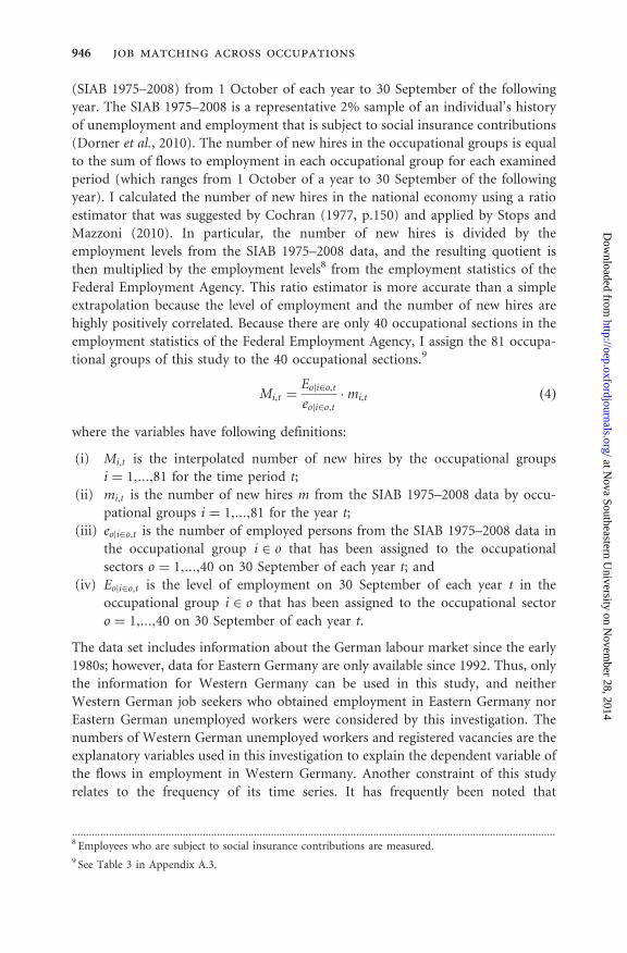
(SIAB 1975–2008) from 1 October of each year to 30 September of the following

year. The SIAB 1975–2008 is a representative 2% sample of an individual’s history

of unemployment and employment that is subject to social insurance contributions

(Dorner et al., 2010). The number of new hires in the occupational groups is equal

to the sum of flows to employment in each occupational group for each examined

period (which ranges from 1 October of a year to 30 September of the following

year). I calculated the number of new hires in the national economy using a ratio

estimator that was suggested by Cochran (1977, p.150) and applied by Stops and

Mazzoni (2010). In particular, the number of new hires is divided by the

employment levels from the SIAB 1975–2008 data, and the resulting quotient is

then multiplied by the employment levels8 from the employment statistics of the

Federal Employment Agency. This ratio estimator is more accurate than a simple

extrapolation because the level of employment and the number of new hires are

highly positively correlated. Because there are only 40 occupational sections in the

employment statistics of the Federal Employment Agency, I assign the 81 occupa-

tional groups of this study to the 40 occupational sections.9

Mi,t ¼Eoji2o,t

eoji2o,t�mi,t ð4Þ

where the variables have following definitions:

(i) Mi,t is the interpolated number of new hires by the occupational groups

i ¼ 1,:::,81 for the time period t;

(ii) mi,t is the number of new hires m from the SIAB 1975–2008 data by occu-

pational groups i ¼ 1,:::,81 for the year t;

(iii) eoji2o,t is the number of employed persons from the SIAB 1975–2008 data in

the occupational group i 2 o that has been assigned to the occupational

sectors o ¼ 1,:::,40 on 30 September of each year t; and

(iv) Eoji2o,t is the level of employment on 30 September of each year t in the

occupational group i 2 o that has been assigned to the occupational sector

o ¼ 1,:::,40 on 30 September of each year t.

The data set includes information about the German labour market since the early

1980s; however, data for Eastern Germany are only available since 1992. Thus, only

the information for Western Germany can be used in this study, and neither

Western German job seekers who obtained employment in Eastern Germany nor

Eastern German unemployed workers were considered by this investigation. The

numbers of Western German unemployed workers and registered vacancies are the

explanatory variables used in this investigation to explain the dependent variable of

the flows in employment in Western Germany. Another constraint of this study

relates to the frequency of its time series. It has frequently been noted that

..........................................................................................................................................................................8 Employees who are subject to social insurance contributions are measured.9 See Table 3 in Appendix A.3.



niversity on Novem


Dow

nloaded from



information about the dynamic changes in the numbers of unemployed workers

and vacancies is lost if yearly data are used; consequently, the estimation results

could be biased (see Petrongolo and Pissarides, 2001, for a broader discussion).

However, I am forced to neglect this issue because data with greater frequencies are

not available for the observed period.

Table 1 presents descriptive statistics for the aggregated stocks and flows from the

data.

4. Empirical strategy and results4.1 An occupational ‘topology’

The empirical approach of this work is based on the idea that cross-sectional units

interact with others; this interaction effect implies that the average behaviour in a

group influences the behaviours of those who constitute the group (Manski, 1993;

Elhorst, 2010). Analogously to a regional topology, which depends on region

adjacency, I derive an ‘occupational group topology’ that relies on the similarities

between occupational groups, in accordance with Matthes et al. (2008).10

The approach in Matthes et al. (2008) is to aggregate occupational groups that

are somewhat ‘similar’ or ‘homogeneous’ according to the KldB 88 into occupa-

tional segments (Berufssegmente), following the concept outlined in an earlier

version of Gathmann and Schonberg (2010). In accordance with this approach,

occupational groups at the three-digit level11 are assumed to be similar if they are

alternatives in recruitment decisions by firms or in job search decisions by potential

employees. This information is available from the Federal Employment Agency and

Table 1 Descriptive statistics

Average 1982–2007(in numbers)

Share (%)

Labour market stocksLabour force E þ U 25,436,839 100.00

Employed E 23,172,935 91.10Unemployed U 2,263,904 8.90

Registered vacancies V 277,831 1.09................................................................................................................................................................

Flows in employment M 5,595,605

Note: The averaged stocks by year were calculated during the course of this study. Data sources: the data

centre of the statistics department of the Federal Employment Agency and the SIAB 1975–2008.

..........................................................................................................................................................................10 See Table 4 in Appendix A.3.11 The German occupational classification scheme 88 (KldB 88) code is a hierarchical construction that

incorporates the following levels (from lowest to highest): occupational classes, which have a four-digit

code; occupational orders, which have a three-digit code; occupational groups, which have a two-digit-

code; and occupational ranges, which have a one-digit code. Under this classification scheme, a given

occupational range consists of certain occupational groups, each of which consists of certain occupa-

tional orders, where each of the latter consists of certain occupational classes.

m. stops 947


niversity on Novem


Dow

nloaded from




its Central Occupational File (Federal Employment Agency, 2010). To identify the

similarities amongst given occupational groups, the Federal Employment Service

has analysed not only the specific skills, licences, certificates, and knowledge re-

quirements but also the typical tasks and techniques involved in each occupational

group (Matthes et al., 2008).12

I transform the results for occupational groups at the three-digit level into oc-

cupational groups on the two-digit level; this transformation is possible due to the

hierarchical structure of the occupational classification scheme.13 Based on this

information, I construct a symmetric 81� 81 first-order contiguity weight matrix

W in which a value of 1 reflects correlations between similar occupational groups.

The diagonal elements are set to 0 since it cannot be assumed that a occupational

group is neighboured to itself; furthermore each occupational group is considered

separately from other similar occupational groups in the empirical model. Finally,

after the weight matrix is row-normalized, it can be used to calculate weighted

averaged numbers of unemployed and vacancies in similar occupational groups.

Thus, Uis (Vis) is the product of the ith 1� 81 row vector wi of the weight matrix W

and the 81� 1 column vector of the numbers of unemployed U (vacancies V) in

each occupational group:

Uis � wiU ¼X81

j¼1

ðwijUjÞ , and Vis � wiV ¼X81

j¼1

ðwijVjÞ

One restriction of this approach must be noted. Some two-digit groups are not

assigned to only one occupational segment because they contain particular three-

digit groups that belong to one segment and other three-digit groups that belong to

another segment.14 However, these occupational groups may be regarded as occu-

pations that are similar to more than one segment (e.g., segment A and segment B)

because they include certain tasks or qualifications that are only found in segment

A and other tasks or qualifications that are only found in segment B. Therefore,

though segments A and B are linked by an occupational group, they are not

necessarily similar.

4.2 Estimation approach and results

To examine the influences of exogenous regressors in other occupational groups,

I use the logarithmic version of the model in eq. (3) considering a panel data

structure with observation periods t:

log Mi,t ¼ log Ai þ �U log Ui,t þ �V log Vi,t þ �U log Uis,t þ �V log Vis,t ð5Þ

..........................................................................................................................................................................12 More details about the methodology can be found in Online Appendix A.4.13 As mentioned, the results of this procedure are summarized in Table 4 in Online Appendix A.3.14 For example, consider occupational group 63, ‘technical specialist’, in Table 4 in Online Appendix A.3.

This group is assigned to ‘Miner/chemical occupations’; ‘Glass, ceramic, paper production’; and

‘Construction’.



niversity on Novem


Dow

nloaded from







At this stage, I present the model, assuming the availability of perfect informa-

tion about job searchers, vacancies, and new hires. Subsequently, to overcome

several shortcomings of the available data, I complement the model with a

recession and a time trend variable. In the first step of model construction, I

apply a pooled ordinary least squares (OLS) estimation. This model is used as a

reference for previous studies, such as those of Fahr and Sunde (2004) or Stops and

Mazzoni (2010). This estimator is based on two further important assumptions: (i)

equality of the matching function parameters across all occupational groups, and

(ii) the stationarity of the time series used. In the second step of the estimation, I

relax the assumption of equality of the intercept by applying a fixed effects (FE)

estimator. Finally, I relax assumption (ii) by applying a pooled mean-group model,

which is an approach that was introduced by Pesaran et al. (1999).

4.3 Pooled OLS and FE estimators

The pooled OLS and FE models can be expressed, respectively, using the following

regression equation with additional control variables and i.i.d. error terms �i,t :

log Mi,t ¼Ai þ �U log Ui,t þ �V log Vi,t þ �U log Uis,tÞ þ �V log Vis,t þ � � �

� � � þ !t þ �GDPcyc þ �i,t

ð6Þ

In accordance with the literature (LeSage and Pace, 2009, p.180), �V and �U can be

interpreted as direct effects on the number of matches, and �V and �U can be

interpreted as indirect effects (of the average number of unemployed workers in

similar occupational groups) on the number of matches. With respect to the field of

labour market theory, it is important not only to compare the impacts of vacancies

and unemployed workers on the matching process but also to analyse returns to

scale in terms of the sum of the matching elasticities. LeSage and Pace, (2009, p.34)

demonstrate that for the simple case of models with cross-sectional dependence

regressors (SLX models), such as those presented in this article, the (average) total

elasticity is simply the sum of the (direct) elasticities, �V and �U , and the indirect

elasticities, �V and �U . Therefore, to analyse the returns to scale of the estimated

matching functions, I provide a Wald test with the null hypothesis that the sum of

all direct and indirect elasticities is unity.15 Amongst others, Berman (1997) argues

that (monthly) numbers of the unemployed and vacancies are reduced by every

hiring, eventually producing a downwards bias in the estimated elasticities. Several

studies for different countries based on elasticity estimations without restrictions

on returns to scale empirically confirm this conjecture (see, e.g., Burda and

Wyplosz, 1994; Fahr and Sunde, 2004; Stops and Mazzoni, 2010). In fact, in this

article, a further potential source of underestimated elasticities is addressed,

namely, the omission of job searchers and vacancies in similar occupational groups.

In the pooled OLS version of the model, the ‘augmented’ productivity coefficient

Ai is equal across the occupational groups, whereas the value of this coefficient may

..........................................................................................................................................................................15 H0: �U þ �V þ �U þ �V ¼ 1 versus Ha: �U þ �V þ �U þ �V 6¼ 1.

m. stops 949


niversity on Novem


Dow

nloaded from


vary in the FE version of the model. Furthermore, the model contains a trend

coefficient, !, that may be interpreted as an indicator of the average development

of matching productivity during the observation period.

Note that the observable numbers of vacancies and unemployed are proxies for

all job searchers and vacancies in the labour market. The use of these proxies could

produce biased estimates (Broersma and van Ours, 1999; Anderson and Burgess,

2000; Fahr and Sunde, 2005; Sunde, 2007). Therefore, Anderson and Burgess

(2000) propose interpreting the empirical matching elasticities as quantities

obtained from a ‘reduced’ model. However, the total number of vacancies might

be found if the ratios of observable vacancies16 to total vacancies were known.

These ratios are occasionally reported (Heckmann et al., 2009), but data for the

entire observation period are not available. However, Franz (2006) reports that

these ratios exhibit partially counter-cyclical characteristics. This finding can be

used to obtain the unbiased coefficient of the matching elasticity of vacancies.

Therefore, I complement the model by incorporating the cyclical component of

the logarithm of German real gross domestic product GDPcyc calculated using the

Hodrick-Prescott filter (Hodrick and Prescott, 1997).17 In accordance with the

work of Franz (2006), the coefficient of the GDPcyc is expected to be positive.

In columns (1) to (4) of Table 2, I present the results for the pooled OLS and FE

models including one version of each model containing cross-sectional lags of

exogenous regressors and one version of each model that does not include these

lags to allow comparisons between those specifications.

Robust standard errors are calculated in accordance with Huber and White.

Information criteria are reported, including the Akaike information criterion

(AIC; Akaike, 1974) and the Bayesian information criterion (BIC; Schwarz,

1978). According to the AIC and BIC, models with the cross-sectional lags of the

exogenous regressors should be preferred over models without such lags.

The matching elasticities of the unemployed workers and vacancies are signifi-

cantly positive and robust in all variations of the model; however, these elasticities

are rather small in the FE models. The positive coefficient of the cyclical component

of the real GDP and the negative parameter of the trend are robust for all of the

models except for the pooled OLS estimation.

The parameters measuring the effect of the unemployed from other occupational

groups, �U , are significant, positive, and robust in the pooled OLS model but not in

the FE model, in which �U is small and insignificant. The coefficients measuring the

impact of vacancies in other occupational groups, �U , are also quite small and

insignificant in both the pooled OLS model and the FE model.18 Accordingly, the

null of the Wald test that both coefficients are simultaneously zero must be rejected

for the pooled OLS model but not for the FE model. The results of the pooled OLS

..........................................................................................................................................................................16 These observable vacancies are those registered by the Federal Employment Service; employers are not

obliged to register vacancies.17 Detailed considerations are provided in Appendix A.5.18 Some variations of both models corroborate these results; compare with Appendix A.6.



niversity on Novem


Dow

nloaded from




estimations indicate a positive relationship between new hires in an occupational

group and unemployed workers in similar occupational groups. There is no robust

indication that vacancies in similar occupational groups have an impact. The FE

model does not reveal any impact from vacancies and unemployed in similar occu-

pational groups. Moreover, the null of the Wald test for constant returns to scale

must be rejected for all of the variants of the pooled OLS and FE models.

4.4 Stationarity and the pooled mean-group model

The properties of the panel variables used are important to ensure that the

correct estimator is applied. Blanchard and Diamond (1989, p.55) report the

Table 2 The results for the matching equation

(1) (2) (3) (4) (5) (6)Dep. variable log M log M log M log M � log M � log M

PooledOLS i

PooledOLS ii

FE i FE ii PMG i PMG ii

�U 0.440*** 0.458*** 0.192** 0.189*** 0.411*** 0.493***(0.025) (0.022) (0.080) (0.071) (0.045) (0.038)

�V 0.389*** 0.377*** 0.210*** 0.236*** 0.238*** 0.255***(0.020) (0.017) (0.049) (0.041) (0.027) (0.019)

�U 0.187*** �0.014 0.358***(0.038) (0.076) (0.075)

�V �0.059 0.077 0.133***(0.036) (0.066) (0.039)

Trend �0.013*** �0.012*** �0.010*** �0.008** �0.044*** �0.032***(0.002) (0.002) (0.003) (0.003) (0.003) (0.002)

GDPcyc 4.746*** 2.932** 1.658*** 2.248*** 12.212*** 9.757***(1.243) (1.198) (0.500) (0.807) (1.419) (1.139)

� �0.240*** �0.263***(0.020) (0.023)

Constant 2.218*** 3.552*** 6.725*** 7.002*** 0.130*** 1.112***(0.276) (0.127) (0.967) (0.760) (0.016) (0.089)

Observations 2,106 2,106 2,106 2,106 1,944 1,944ll �1,747 �1,770 �303.3 �311.1 1,874 1,865AIC 3,507 3,549 618.6 630.2 �3,721 �3,708BIC 3,547 3,578 652.5 652.8 �3,649 �3,647

Wald test (Prob> F) 0.132 0.000 0.000 0.000 0.086 0.000H(0): constantreturns to scaleWald test (Prob>�2) 0.000 0.503 0.000H(0): �U and �V aresimultaneously 0

Notes: (1) pooled OLS and FE model: robust standard errors in parentheses. Akaike information criteria

(AIC), Bayesian information criteria (BIC) on the base of the likelihood (ll) derived by the estimation

results. (2) FE and PMG model: constant = average of fixed effects. (3) PMG model: short-run coeffi-

cients are not reported here; further results can be found in Table 3. AIC, BIC on the base of the

maximum likelihood estimation (ll). *** p< 0.01, ** p< 0.05, * p< 0.1.

m. stops 951


niversity on Novem


Dow

nloaded from


results of augmented Dickey-Fuller tests that reject the null of nonstationarity.

However, these researchers could not show the existence of cointegration

in the observed data. Entorf (1998, p.79) confirmed that unit roots are

seldom found in panel time series for certain metrics such as new hires,

vacancies, and unemployed workers. Fahr and Sunde (2004) use a stationarity

test of Hadri (2000) with a null of stationarity and find that the null could not

be rejected for their data. Stops and Mazzoni (2010) employ the same test for

similar data with more observation time points and demonstrate that the null

must be rejected.

I apply the same test, and the results indicate again that the assumption of

stationarity should not be maintained. The null of stationarity must therefore be

rejected for all time series of new hires, vacancies, and unemployed workers. By

contrast, the null could not be rejected for the first-order difference series because

of the possibility of homoscedastic standard errors.19 Thus, the time series are likely

to be integrated of order 1. Furthermore, from a theoretical perspective, there is a

long-run linear relationship between the logarithm of new hires and both

unemployed workers and vacancies, and it can be reasonably assumed that these

variables are co-integrated. Therefore, I apply the pooled mean-group model

(PMG) proposed by Pesaran et al. (1999), which models these data characteristics

well (Baltagi, 2002, p.245). The basis of the PMG estimator is an autoregressive

distributive lag (l, q1, q2, . . . , qk) model (ARDL model) with q ¼ q1 ¼ q2 ¼ ::: ¼ qk.

This model is reparameterized in a error correction form. In this study, I use a

reparameterized ARDL(1,1,1) model as follows:

� log Mi,t ¼�i½log Mi,t�1 � ð�U log Ui,t þ �V log Vi,t þ :::

:::þ �U log Uis,t þ �V log Vis,tÞ þ �Ui � log Ui,t

þ �Vi �Vi,t þ Ai þ �i,t

ð7Þ

In addition to the pooled OLS and FE estimators, the following variables are now

implemented:

(i) � log Mi,t are the first-order backwards differences of the logarithm of the

flow in employment,

(ii) � log Ui,t and � log Vi,t are the first-order backwards differences of the

logarithm of unemployed persons and vacancies, and

(iii) �Ui and �V

i are the regression coefficients of these differences.

There is an adjustment process for log Mi,t; the error-correction term �i on the

right-hand side of eq. (7) denotes the speed of adjustment, whereas the term in the

square brackets represents deviations from the long-run equilibrium. If �i is equal

to the null, then there is no long-run equilibrium between the dependent and

..........................................................................................................................................................................19 This conclusion is also true with respect to heteroscedasticity of the residuals, with an exception for

unemployed workers at a significance level of 10%. Please compare the results in Table 10 in

Appendix A.6.



niversity on Novem


Dow

nloaded from




independent variables. A significant negative parameter indicates that the variables

tend to a long-run steady state.

The PMG estimator includes the FE and short-run dynamics of the variables for

each occupational group i and requires the long-term coefficients to be equal across

all occupational groups i. The PMG model in eq. (7) is nonlinear in its parameters

�i and ð�U ,�V Þ. Therefore, a maximum likelihood estimator is applied (Pesaran

et al., 1999, p.465).20 Columns (5) and (6) of Table 2 presents the results for the

long-run coefficients and the averaged error-correction term for two variations of

the model, one version with cross-sectional lags of the exogenous regressors and

one version without. In addition, for these two models, the null hypothesis of the

Wald test, stating that �U and �V are simultaneously equal to 0, must be rejected.

Given the information criteria examined, the model with the cross-sectional lags of

regressors should be preferred to the model without such lags.

Table 3 contains all the model results. The long-run elasticities of vacancies and

unemployed workers, the exogenous regressors, the cyclical component of real

GDP, and the trend can be found in the upper part of Table 3. At the bottom of

the table, the following quantities appear: the error-correction term �, the averages

of the estimated short-term parameters for each occupational group, and the

average fixed effect A (denoted as Constant, Pesaran et al., 1999, S. 626).

The error-correction term � is significant and negative for all variants of the

model. This result indicates the existence of movements against deviations from the

long-run equilibrium and therefore implies the existence of stable relationships

between matches and both unemployed workers and vacancies. The long-term

coefficients �U , �V , �U , �V , and GDPcyk are positive, and the trend T is negative

and significantly different from 0; the latter result implies that on average the

augmented matching productivity decreased during the observation period.

These results are robust for all estimated model variations.21 The effect of

unemployed workers on matches is larger than the effect of vacancies, even after

accounting for the 95% confidence intervals of �V and �U . This finding is in

accordance with other studies for Germany (Burda and Wyplosz, 1994; Fahr and

Sunde, 2004; Stops and Mazzoni, 2010). The indirect effects of unemployed and

vacancies in similar occupational groups (�U , �V ) are each smaller than the direct

effects of their counterparts (�U , �V ). This implies for each occupational group that

changes in the number of unemployed or vacancies in the same occupational group

have a greater effect on new hires in that occupational group than do changes in the

number of unemployed or vacancies in similar occupational groups.22 For all of the

..........................................................................................................................................................................20 See Appendix A.7.21 There is one exception: �U takes a negative sign after excluding the trend T. However, this model

specification would at least be preferred according to the information criteria reported.22 At this stage, it may be beneficial to enquire about the empirical impact of changes in nonsimilar

occupational groups, and it may be expected that there is no impact. However, such a direct falsification

test appears to be inadequate because the resulting estimates may partially reveal only common trends or

shocks to the single occupational unemployment and vacancy time series. Furthermore, the results

should instead be interpreted as correlations rather than elasticities, because the used weight matrices

m. stops 953


niversity on Novem


Dow

nloaded from



examined model variations, there is a significant positive relationship between

changes in the number of new hires and changes in the number of vacancies, in

Table 3 The results of the PMG estimations that use � log M as the dependent

variable

(1) (2) (3) (4) (5) (6)PMG 1 PMG 2 PMG 3 PMG 4 PMG 5 PMG 6

Long-run coefficients�U 0.411*** 0.420*** 0.500*** 0.493*** 0.381*** 0.680***

(0.045) (0.044) (0.039) (0.038) (0.030) (0.055)�V 0.238*** 0.282*** 0.211*** 0.255*** 0.296*** -0.036

(0.027) (0.021) (0.025) (0.019) (0.017) (0.033)�U 0.358*** 0.306*** 0.026 -0.359***

(0.075) (0.072) (0.044) (0.073)�V 0.133*** 0.072** 0.053** 0.017

(0.039) (0.032) (0.025) (0.043)Trend �0.044*** �0.039*** �0.033*** �0.032*** �0.028***

(0.003) (0.003) (0.002) (0.002) (0.002)GDPcyc 12.212*** 11.971*** 10.444*** 9.757*** 15.494***

(1.419) (1.387) (1.189) (1.139) (1.934)� �0.240*** �0.244*** �0.257*** �0.263*** �0.329*** �0.180***

(0.020) (0.021) (0.022) (0.023) (0.035) (0.015)Short-run coefficients&�M�1

1 �0.107*** �0.097*** �0.096*** �0.088*** �0.040 �0.095***(0.022) (0.022) (0.023) (0.023) (0.025) (0.024)

��U0 �0.172*** �0.180*** �0.171*** -0.180*** -0.226*** -0.079***

(0.030) (0.030) (0.030) (0.030) (0.034) (0.028)��U�1 �0.061*** �0.065*** �0.055** �0.058** �0.065*** 0.002

(0.023) (0.023) (0.023) (0.023) (0.023) (0.023)��V

0 0.044*** 0.043*** 0.051*** 0.046*** 0.024 0.118***(0.014) (0.014) (0.014) (0.014) (0.017) (0.015)

��V�1 0.040*** 0.041*** 0.046*** 0.044*** 0.040** 0.103***

(0.014) (0.014) (0.014) (0.014) (0.016) (0.012)Constant 0.130*** 0.416*** 1.004*** 1.112*** 1.398*** 1.346***

(0.016) (0.030) (0.077) (0.089) (0.144) (0.105)

Observations 1,944 1,944 1,944 1,944 1,944 1,944ll 1,874 1,870 1,867 1,865 1,826 1,789AIC �3,721 �3,716 �3,709 �3,708 �3,628 �3,554BIC �3,649 �3,649 �3,642 �3,647 �3,561 �3,487

Wald test (Prob> F) 0.0857 0.906 0.000 0.000 0.000 0.000H(0): constant returns to scale

Notes: Standard errors in parentheses. ***p< 0.01, **p< 0.05, *p< 0.1. Constant = average of fixed

effects.

..........................................................................................................................................................................of nonsimilar occupational groups are neither theoretically nor empirically based. I provide an indirect

falsification test that uses the same model framework but compares shock-adjusted correlations of the

unemployed and vacancies in similar occupational groups and new hires with those of randomly selected

nonsimilar occupational groups. The results show that the estimated correlations for the empirically

based selection of similar occupational groups are higher than those for the nonsimilar occupational

groups. Details can be found in Appendix A.8.



niversity on Novem


Dow

nloaded from



addition to a significant negative relationship between changes in the number of

new hires and changes in the number of unemployed workers.

The positive relationships between new hires in an occupational group and

vacancies and unemployed workers in similar occupational groups have

important implications for estimations of the matching efficiencies of

unemployed workers and vacancies. In particular, this result indicates that these

efficiencies are determined not only by the numbers of unemployed workers and

vacancies in the same occupational group but also by the numbers of unemployed

workers and vacancies in similar occupational groups.

5. ConclusionsThis article analyses matching processes in occupational labour markets in terms of

classes of jobs that share commonalities in required qualifications and tasks. All

previous studies in this field have been based on the assumption that job search and

job matching processes occur separately in each occupational labour market, but

this assumption is theoretically and empirically unreasonable. From the perspec-

tives of both potential workers and employers, optimal search intensities in each

occupational labour market are weighted against the expected gains and costs of

searching, the latter of which could be the (additional) financial burden of the

training that is required for a change from one occupation to another.

Therefore, workers who are prepared to work in a certain occupation may

decide to search for a job in other occupations if the resulting search costs are

not too high relative to the expected gains; similarly, firms with vacancies in a

certain occupation may decide to search for workers currently in other occupations,

if such workers might be viable alternatives. This reasoning implies that the

processes of job search and matching occur not only in each occupational labour

market but also across certain occupational labour markets. I support this

prediction through observations of occupational changes that are obtained from

German microdata.

I argue that these findings have important implications for estimating the macro-

economic matching function because an explanation of matches (in terms of new

hires) in a given occupation requires consideration not only of vacancies and

unemployed workers in the occupation of interest but also of vacancies and

unemployed workers in other relevant occupations. I use information regard-

ing similarities of occupational groups with respect to their capacities to function

as alternatives in the processes of worker and job search to construct an ‘occupa-

tional topology’. Based on this topology, it is possible to calculate, for each occu-

pational group, average vacancies and unemployed in similar occupations. Finally, I

estimate an augmented matching function using pooled OLS, FE, and pooled

mean-group models that include cross-sectional dependency lags of regressors in

terms of vacancies and unemployed workers in similar occupational groups.

The results of this study indicate considerable dependencies between similar

occupational groups in the matching process. I show that there are significant

m. stops 955


niversity on Novem


Dow

nloaded from


and positive matching elasticities of vacancies and unemployed in similar occupa-

tional groups, which is a finding that has important implications for estimating the

matching elasticities of unemployed workers and vacancies; such elasticities are

determined not only by the number of unemployed workers and vacancies in the

occupational group of interest but also by the number of unemployed workers and

vacancies in other occupational groups. Furthermore, the results reveal that returns

to scale that are implied by the estimation results for the pooled mean-group

model—which considers cross-sectional dependency—are constant on a signifi-

cance level of 5%. In sum, the findings of this study suggest that an augmented

empirical matching function that considers job and worker searches across different

occupational labour markets should be employed to obtain unbiased elasticity

estimates.

Supplementary materialSupplementary material is available online at the OUP website.

AcknowledgementsI thank two anonymous referees, the Associate Editor Ken Mayhew, Wolfgang Dauth,Domenico Depalo, Peter Dolton, Alexandra Fedorets, Therry Gregory, FranziskaLottmann, Britta Matthes, Joachim Moeller, Friedrich Poeschel, Martina Rebien, and EnzoWeber for valuable comments and suggestions. I am also grateful for the feedback providedby various participants at the Macro Labour Seminar, Nuremberg; the Economic Seminar atRoyal Holloway, the University of London; and the conferences of the Spatial EconometricsAssociation, the European Regional Science Association, and the Verein fuer Socialpolitik.The usual disclaimer applies.

ReferencesAkaike, H. (1974) A new look at the statistical model identification, IEEE Transactions onAutomatic Control, 19, 716–23.

Anderson, P.M. and Burgess, S.M. (2000) Empirical matching functions: estimation andinterpretation using state-level data, Review of Economics and Statistics, 82, 93–102.

Baltagi, B.H. (2002) Econometrics, 3rd edn, Springer, Berlin.

Berman, E. (1997) Help wanted, job needed: estimates of a matching function fromemployment service data, Journal of Labor Economics, 15, 251–292.

Blanchard, O.J. and Diamond, P. (1989) The Beveridge curve, Brookings Papers on EconomicActivity, 20, 1–76.

Broersma, L. and van Ours, J. (1999) Job searchers, job matches and the elasticity ofmatching, Labour Economics, 6, 77–93.

Burda, M.C. and Profit, S. (1996) Matching across space: evidence on mobility in the CzechRepublic, Labour Economics, 3, 255–78.

Burda, M.C. and Wyplosz, C.A. (1994) Gross worker and job flows in Europe, EuropeanEconomic Review, 38, 1287–315.



niversity on Novem


Dow

nloaded from



Cochran, W.G. (1977) Sampling Techniques, 3rd edn, Wiley series in probability and math-

ematical statistics, Wiley, New York.

Dauth, W., Hujer, R., and Wolf, K. (2010) Macroeconometric evaluation of active labour

market policies in Austria. IZA Discussion Paper No. 5217, IZA, Bonn.

Dorner, M., Heining, J., Jacobebbinghaus, P., and Seth, S. (2010) Sample of Integrated

Labour Market Biographies (SIAB) 1975–2008, FDZ-Datenreport No. 1, IAB, Nuremberg.

Elhorst, J.P. (2010) Applied spatial econometrics: raising the bar, Spatial Economic Analysis,

5, 9–28.

Entorf, H. (1994) Trending time series and spurious mismatch, Beitrage zur angewandten

Wirtschaftsforschung, Institut fur Volkswirtschaftslehre und Statistik, Mannheim.

Entorf, H. (1998) Mismatch Explanations of European Unemployment: A Critical Evaluation,

European and Transatlantic Studies, Springer, Berlin.

Fahr, R. and Sunde, U. (2004) Occupational job creation: patterns and implications, Oxford

Economic Papers, 56, 407–35.

Fahr, R. and Sunde, U. (2005) Job and vacancy competition in empirical matching

functions, Labour Economics, 12, 773–80.

Fahr, R. and Sunde, U. (2006) Spatial mobility and competition for jobs: some theory and

evidence for Western Germany, Regional Science and Urban Economics, 36, 803–25.

Federal Employment Agency (2010) Zentrale Berufedatei (Central occupational file), http://

berufenet.arbeitsagentur.de (accessed 16 April 2014).

Fitzenberger, B. and Spitz, A. (2004) Die Anatomie des Berufswechsels: Eine empirische

Bestandsaufnahme auf Basis der BIBB/IAB-Daten 1998/1999, ZEW-Discussion Paper No.

04-05, ZEW, Mannheim.

Franz, W. (2006) Arbeitsmarktokonomik, 6th edn, Springer-Lehrbuch, Springer, Berlin.

Gathmann, C. and Schonberg, U. (2010) How general is human capital? A task-based

approach, Journal of Labor Economics, 28, 1–49.

Hadri, K. (2000) Testing for stationarity in heterogenous panel data, Econometrics Journal, 3,

148–61.

Heckmann, M., Kettner, A., and Rebien, M. (2009) Einbruch in der Industrie - soziale

Berufe legen zu: Offene Stellen im IV, Quartal 2008, IAB-Kurzbericht No. 11, IAB,

Nuremberg.

Hodrick, R.J. and Prescott, E.C. (1997) Postwar US business cycles: an empirical investiga-

tion, Journal of Money, Credit and Banking, 29, 1–16.

Kambourov, G. and Manovskii, I. (2009) Occupational specificity of human capital,

International Economic Review, 50, 63–115.

Kangasharju, A., Pehkonen, J., and Pekkala, S. (2005) Returns to scale in a matching model:

evidence from disaggregated panel data, Applied Economics, 37, 115–18.

LeSage, J.P. and Pace, R.K. (2009) Introduction to Spatial Econometrics, vol. 196 of Statistics,

CRC Press, Boca Raton.

Lottmann, F. (2012) Spatial dependencies in German matching functions, Regional Science

and Urban Economics, 42, 27–41.

Manski, C.F. (1993) Identification of endogenous social effects: the reflection problem,

Review of Economic Studies, 60, 531–42.

m. stops 957


niversity on Novem


Dow

nloaded from

http://berufenet.arbeitsagentur.de

http://berufenet.arbeitsagentur.de


Matthes, B., Burkert, C., and Biersack, W. (2008) Berufssegmente: Eine empirisch fundierteNeuabgrenzung vergleichbarer beruflicher Einheiten, IAB-Discussion Paper No. 35, IAB,Nuremberg.

Mora, J.J. and Santacruz, J.A. (2007) Emparejamiento entre desempleados y vacantes paraCali: un analisis con datos de panel (Unemployment and vacancies in a matching model forCali: a panel data analysis; with English summary), Estudios Gerenciales, 23, 85–91.

Pesaran, M.H., Shin, Y., and Smith, R.P. (1999) Pooled mean group estimation of dynamicheterogeneous panels, Journal of the American Statistical Association, 94, 621–34.

Petrongolo, B. and Pissarides, C. (2001) Looking into the black box: a survey of thematching function, Journal of Economic Literature, 39, 390–431.

Pissarides, C.A. (2000) Equilibrium Unemployment Theory, 2nd edn, MIT Press, Cambridge.

Rogerson, R., Shimer, R., and Wright, R. (2005) Search-theoretic model of the labor market:a survey, Journal of Economic Literature, 43, 959–88.

Schmillen, A. and Moller, J. (2012) Distribution and determinants of lifetime unemploy-ment, Labour Economics, 19, 33–47.

Schwarz, G. (1978) Estimating the dimension of a model, Annals of Statistics, 6, 461–64.

Seibert, H. (2007) Wenn der Schuster nicht bei seinem Leisten bleibt. . ., IAB-KurzberichtNo. 1, IAB, Nuremberg.

Shimer, R. (2005) The cyclical behavior of equilibrium unemployment and vacancies,American Economic Review, 95, 25–49.

Stops, M. and Mazzoni, T. (2010) Job matching on occupational labour markets, Journal ofEconomics and Statistics (Jahrbucher fuer Nationalokonomie und Statistik), 230, 287–312.

Sunde, U. (2007) Empirical Matching Functions: Searchers, Vacancies, and (Un-) biasedElasticities, Economica, 74, 537–560.

Yashiv, E. (2007) Labor search and matching in macroeconomics, European EconomicReview, 51, 1859–95.



niversity on Novem


Dow

nloaded from


Documents

Job matching across occupational labour markets