Job Loss, Family Ties and Regional Mobility

0

Job Loss, Family Ties and Regional Mobility*

Kristiina Huttunen Department of Economics

Aalto University School of Economics, HECER and IZA [email protected]

Jarle Møen

Department of Finance and Management Science Norwegian School of Economics and Business Administration

[email protected]

Kjell G. Salvanes Department of Economics

Norwegian School of Economics, Statistics Norway, Center for the Economics of Education (CEP) and IZA

[email protected]

Draft, October 2013

ABSTRACT It is well established that displaced workers suffer long-lasting and severe employment and earning losses. Why these losses appear to be so big and so persistent is on other hand not very well understood. For instance, it might be that workers who are affected by big and persistent income effects are immobile for different reasons limiting the search. Hence, the immobility of workers is one of the obstacles for well-functioning labor markets. This paper analyzes the geographic mobility of workers after permanent job loss. We study what affects the likelihood that worker moves away from the region after job loss. We put particular importance to family ties. We find that job displacement increases regional mobility. Family ties are very important for mobility decisions: workers are less likely to move if they have family in the region and some return back home after job loss. When analyzing the post-displacement differences in outcomes we find that movers tend to suffer more severe earning and employment losses after job loss than stayers. The difference is larger for females, and for workers moving away from urban areas and to regions where their parents live. This indicates that movers tend to move for non-economic reasons also: spouse’s work and family ties are very important for mobility decision. Although the overall selection of movers appears to be from the lower tail of the skill distribution in the source regional labor market, we do find some indication of a great deal of heterogeneity in terms of selection depending on the returns to skill in the labor market they move to. Keywords: plant closures, downsizing, regional mobility, earnings, family ties

*We thank seminar participants in Austin, Texas. Huttunen gratefully acknowledge financial support from Finnish Academy. Salvanes and Møen thanks The Norwegian Research council for financial support.

1

1 Introduction

Downsizing and closures of firms is a crucial part of the process of restructuring and

growth of industries including a reallocating of displaced workers between firms and

sectors and across regions (Blanchard and Katz, 1992). However, it is well established

that displaced workers suffer long-lasting and severe employment and earning losses (e.g.

Jacobsen, LaLonde, and Sullivan, 1994; Couch and Placzek, 2010; Eliason and Storrie,

2006; Bender and von Wachter, 2009, Rege, Telle and Votruba, 2010; Huttunen, Møen

and Salvanes, 2010). Why these losses appear to be so big and so persistent is on other

hand not very well understood. For instance, it might be that workers who are affected by

big and persistent income effects are immobile for different reasons limiting the search.

The costs of moving may vary for different reasons such as family responsibilities,

networks etc. Knowledge of whether losses from displacement are strongly connected to

immobile workers will inform policy makers on the importance of developing policy

instruments that induce higher mobility and to smooth restructuring processes.1

This paper makes several contributions to the literature examining the question of why

we see the strong persistence in losses following job displacement. First, to our

knowledge, this is the first study that documents how mobile workers are across regional

labor markets following a permanent job loss, and what factors explain why workers do

not move after job loss. We show the importance of non-economic factors, such as family

ties and family networks, on worker’s mobility decision. We analyze also the selection of

1 Especially, the increased international trade to low cost countries such as China, had had a big impact on downsizing and restructuring of the manufacturing sector during the last couple of decades, see Author, Dorn, Hanson, and Song (2012) for and analysis of the impact on restructuring of regional labor markets for the US, and for an analysis of the China impact on Norway, see Balsvik, Jensen, and Salvanes (2012). Smoothing these processes has a large focus in economic policies (Heinrich, Mueser and Troske, 2010).

2

movers both with respect to individual characteristics and with respect to characteristics

of the labor markets they move between. Secondly, we document how the workers are

doing in terms of earnings, unemployment and the probability of leaving the labor. We

also document how the economic outcomes for the movers compared to non-movers after

displacement depend the characteristics of location where they move to, such as

urban/rural, moving to where they have family ties etc.

The negative employment shock that displaced workers experience is expected to change

incentives to migrate. In the first part of the analysis, we assess to what degree

displacement causes regional mobility using the standard set up in the displacement

literature, where plant exit or downsizing is considered a shock to the individual workers

conditioned on a rich set of pre-displacement variables. Displaced workers are compared

to a control group of non-displaced. A unique feature of our data is that we have rich

information on the location of both parents and siblings of the workers, the age of their

children, and the same for the spouse. Thus, for the displaced we can assess how various

observable demographic variables and family network variables impact regional mobility.

In the second part of the analysis we assess the post-displacement labor market

experience of movers and stayers. Here we use a standard set up in the regional

economics (or across country) literature and specify a fixed effect model comparing

outcomes in the labor market for movers and stayers (Glaeser and Mare, 2001). We focus

both on employment and earnings, as well as income (including disability benefits from

leaving the labor force early) both based on individual and family income. Importantly

3

we also take into account that the living expenses (especially housing) differs a lot across

regional labor markets by using a regional consumer price index. A fixed effect

specification will to a certain extent take out the heterogeneity in skills between movers

and stayers, however, we should basically consider the results on earnings and income as

a combined effect of returns to moving after being displaced and a selection effect.

Fundamentally, question we are dealing with when asses the labor market outcomes for

movers as compared to non-movers among job losers, is whether the movers are

positively or negatively selected. Theoretically the selection of who is moving and who

stay is not obvious. The prediction from the Roy model using comparative advantages in

the Borjas version of the model that selection is that the mover selection is based on not

the absolute but the relative return to skill in the local labor market they move from and

the local labor market they move to (Roy, 1951; Borjas, 1987, 1991; Borjas, Bronars, and

Trejo, 1992). As discussed in Abramitzky, Boustan and Eriksson (2012), this implies

that there might be a difference in the skill of those moving to the a local labor market

where the returns to skill is high as compared to those moving to a local labor market

where the returns to skill is low, both relative to the source local labor market. In the case

of moving to a regional labor market where skills have a relatively higher return, positive

selection of movers is expected as compared to stayers since movers are to a greater

extent from the higher tail of the skill distribution. On the other hand, those who move to

a regional labor market with relatively lower returns to skill as compared to the source

labor market, predicted to be from the lower part of the skill distribution. In our setting,

this means that where in the skill distribution the movers and the stayers are coming from

4

whether we see a bigger or smaller negative earnings and income effects for stayers and

movers. It might well be that the most highly skilled (and highly enumerated workers)

are best rewarded in the same labor market where they are displaced compared to their

alternatives. Hence, stayers may be the most attractive workers and are more easily

employable workers and they do not have to move in order to find a good job.

Furthermore, the movers may be a very heterogeneous group consisting both of

positively and negatively selected workers depending on the skill returns in the labor

market they move to. One way to get at this is to assess the labor market performance for

displaced movers as compared to displaced stayers, when we condition on where the

displaced movers move. In particular, we do two cuts at the data: estimating the outcomes

and persistence of the negative income shock for workers moving to urban versus rural

areas as well as moving back to where the parents or the spouse’s parents live.

As expected, we find that job displacement increases regional mobility. The mobility

increase takes place two years after displacement, and then the difference in mobility

between displaced and non-displaced is fairly constant over time. After two years about

three percent of the displaced workers have migrated to a new region and two percent of

the non-displaced. When conditioning on a large set of pre-displacement variables

including children in school, marriage, and family networks we find that job

displacement increases mobility by 6 percentage point. This effect corresponds to about

30 percent increase in mobility when comparing it to the two percentage migration

average of non-displaced group. We also find that migrating workers are younger, more

educated and more often single as compared to those who stay. Women are more likely to

5

migrate than men. We find that parental proximity and sibling proximity are factors that

strongly reduce migration. When analyzing the post-displacement labor market

experience of movers and stayers, we find that displaced workers who move have

significantly lower re-employment rates than those who stay in the pre-displacement

region. Our fixed effect estimation results indicate that displaced male movers have

larger long-term earnings losses than displaced male stayers. For women, the difference

between stayers and movers is even more pronounced. This might reflect that women are

often so called “tied movers”, and that is the man’s career which determinates families

moving decisions. When splitting the sample to workers who on the basis of their post-

displacement regional status, we find that the negative effect of migration is entirely

driven by people who move to rural region or to region where family members locate.

This indicates that the movers are both positively and negatively selected from the skill

distribution in the regional labor market where they come from. Those negatively

selected and as it appears are moving for non-economic reasons, are willing to suffer

earning losses if they can stay close to their family members.

The rest of the paper is organized as follows: Section 2 presents the institutional set up

and a short literature review. Section 3 lays out the empirical strategy. Section 4 describes

the data sets and the sample construction. Section 5 presents descriptive evidence and

results of the part that analyzes mobility decisions after job loss. Section 6 presents the

results of the analysis that examines how job displacement effects on labor marker

outcomes vary between movers and stayers. Section 7 concludes.

6

2 Literature

It well established that family ties influence worker’s mobility decisions (Mincer, 1978)2.

Mincer (1978) established that it is the net family gain rather than net personal gain that

motivate the migration of households. The possible net loss of a “tied” mover must be

smaller than the net gain of the other spouse to result in a net family gain. Since the

return to migration for families increase less than costs when household size increases,

one would expect families to be less mobile than single individuals. The moving

decisions of families are affected by a number of factors, such as the number of children,

the age of the children and access to schools which the family prefers. Recent research

has also shown that the location of parents and siblings is important. (Kolmar et al., 2002,

and Rainer and Siedler, 2005).

In particular we examine whether parents of the displaced worker or the spouse live in

the local labor market where the displacement incident happens. Proximity to parents

may reduce mobility for more specific reasons. Having parents and siblings close is an

advantage because people in general enjoy the company of their family. Parents may be

elderly and in need of care, or if not elderly, they may help bringing up children by acting

as baby sitters and providing extra non-parental child care (Lin and Rogerson, 1993,

Glaser and Tomassini, 2000). The effect of siblings on the decision to move is a bit more

complicated. Siblings represent a positive incentive to stay for the same reason as

2 Alessina et al. (2010) show that individuals who inherit stronger family ties are less mobile, have

lower wages, and are less often employed.

7

parents, but their presence may also make it easier to move because they are substitute

caretakers for elderly parents. This is pointed out by Konrad et al. (2002) and Rainer and

Seidler (2005).3 Proximity to parents and siblings can also influence worker’s

employment and earnings directly. A family network in the local labor market may aid

workers in finding new employment (Kramarz and Skans, 2011), and family member that

act as baby sitters will make it easier to work long hours.

3 Empirical Specification

The objective of this study is to analyze whether firm restructuring leading to worker job

loss, leads to increased regional mobility, and secondly to provide evidence how

geographic mobility is related to earning losses of displaced workers. We estimate

separate regressions for men and women.

Defining the treatment and control groups

Following the literature we use job displacements as a shock to the individual worker and

analyze how regional mobility is affected. Displaced workers are defined as workers

losing their job following plant close downs and those separated from a plant that reduces

employment by 30 % or more (Jacobsen, Lalonde and Sullivan, 1993, Bender and Von

Wachter, 2009). Furthermore, we add early leavers to the treatment group defined as

those who left the plant up to one year prior to plant closure since we expect them to be

aware of the future closedown. As the control group we use a 30 percent sample of non-

3 These papers are not assessing migration per se, but analyze proximity between siblings and parents. In the models elder children act strategically by choosing to migrate away from parents in need of care.

8

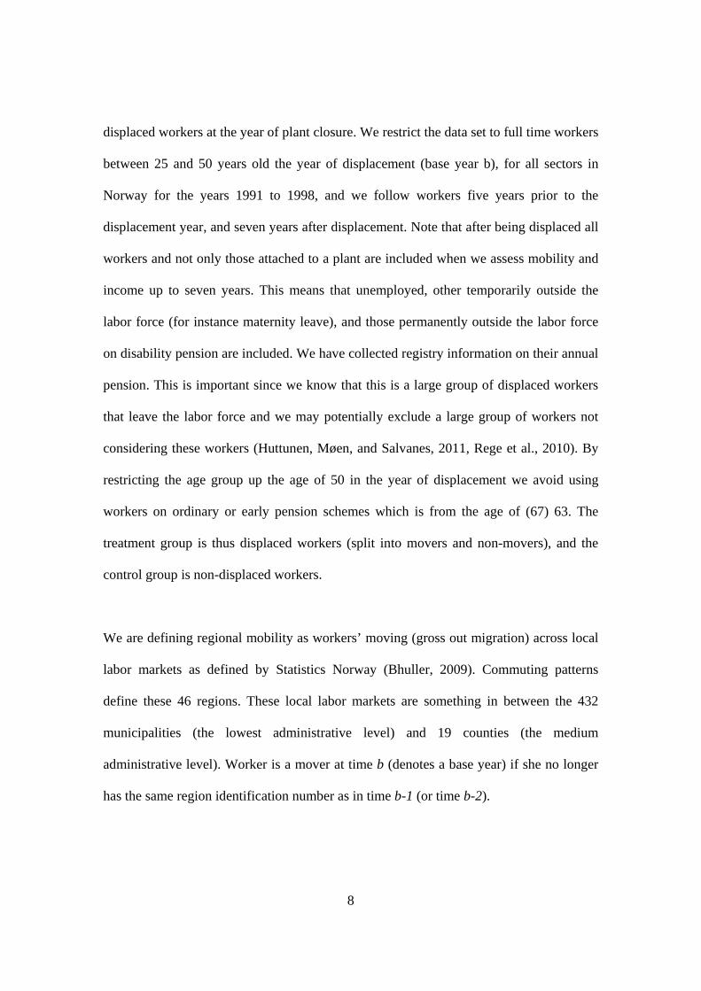
displaced workers at the year of plant closure. We restrict the data set to full time workers

between 25 and 50 years old the year of displacement (base year b), for all sectors in

Norway for the years 1991 to 1998, and we follow workers five years prior to the

displacement year, and seven years after displacement. Note that after being displaced all

workers and not only those attached to a plant are included when we assess mobility and

income up to seven years. This means that unemployed, other temporarily outside the

labor force (for instance maternity leave), and those permanently outside the labor force

on disability pension are included. We have collected registry information on their annual

pension. This is important since we know that this is a large group of displaced workers

that leave the labor force and we may potentially exclude a large group of workers not

considering these workers (Huttunen, Møen, and Salvanes, 2011, Rege et al., 2010). By

restricting the age group up the age of 50 in the year of displacement we avoid using

workers on ordinary or early pension schemes which is from the age of (67) 63. The

treatment group is thus displaced workers (split into movers and non-movers), and the

control group is non-displaced workers.

We are defining regional mobility as workers’ moving (gross out migration) across local

labor markets as defined by Statistics Norway (Bhuller, 2009). Commuting patterns

define these 46 regions. These local labor markets are something in between the 432

municipalities (the lowest administrative level) and 19 counties (the medium

administrative level). Worker is a mover at time b (denotes a base year) if she no longer

has the same region identification number as in time b-1 (or time b-2).

9

Since we are analyzing displacement that occurs in several years, we have a rolling base

year, denoted b as the year of displacement, and b+1 being the first year after and b-1

being the year prior to displacement. We redefine base year accordingly and run pooled

regressions for all base year samples 1991 to 1998.

We restrict our sample to workers with job tenure working at least 20 hours per week for

the three years leading up to displacement, b-3 to b-1. This means that they have

attachment to a firm the 3 years leading up to displacement (and the displacement year),

and had positive earnings from working.

Displacement and regional mobility

We begin by estimating the effect of displacement and background factors on regional

mobility separately for males and females using following specification:

where Dib is an indicator for whether worker i was displaced in a base year, b. Mib+2 is an

indicator for whether worker i's moving status, that is whether the worker lives in a

different region two years after the base year, b+2. Xib is a vector of observable worker,

plant, labor market regions pre-displacement characteristics (from base year 0 if not

mentioned otherwise). They are worker's age, age squared, education split into three

categories, tenure, marital/cohabitation status, number of children and children under 7

ibbibibib XDM 2

10

(preschool age), earnings in years b-4 and b-5, months of employment in years b-4 and b-

5, and dummy for being in education at b-4 and b-5, years individuals have lived in pre-

displacement region by base year b, plant size, indicator variable for having younger

siblings, dummy variable indicating whether parents of the worker or his spouse are

living in the same pre-displacement local labor market, dummy variable indicating

whether sibling of the worker or his spouse are living in the same pre-displacement local

labor market, and the interaction of these two (having spouse in the region*having sibling

in the region), regional unemployment rate, region size. Specification includes also base

year fixed-effects b , base year two-digit NACE industry dummies, and base year region

dummies.

The main variable of interest is the displacement variable Dib. This is a dummy

variable indicating whether a displacement occurs at between the year b and b+1. The

parameter gives the difference in regional mobility between displaced and not-

displaced workers conditional on all pre-displacement controls.

Next we study the importance of observable worker, network and labor market

variables. Family ties are expected to affect workers’ mobility decision as already

discussed. Another dimensions related to families is whether the displaced worker (man

or women) has a spouse or not. We expect that having a spouse reduces regional mobility

since they are working, have networks on their own etc. The effect of job loss on

migration may differ between workers with different education level and between

workers in urban and rural locations. For example, the labor markets for highly educated

workers are generally regionally much larger than those of low educated workers (see

e.g. Machin, Salvanes and Pelkonen, 2011). This indicates that job loss would lead to a

11

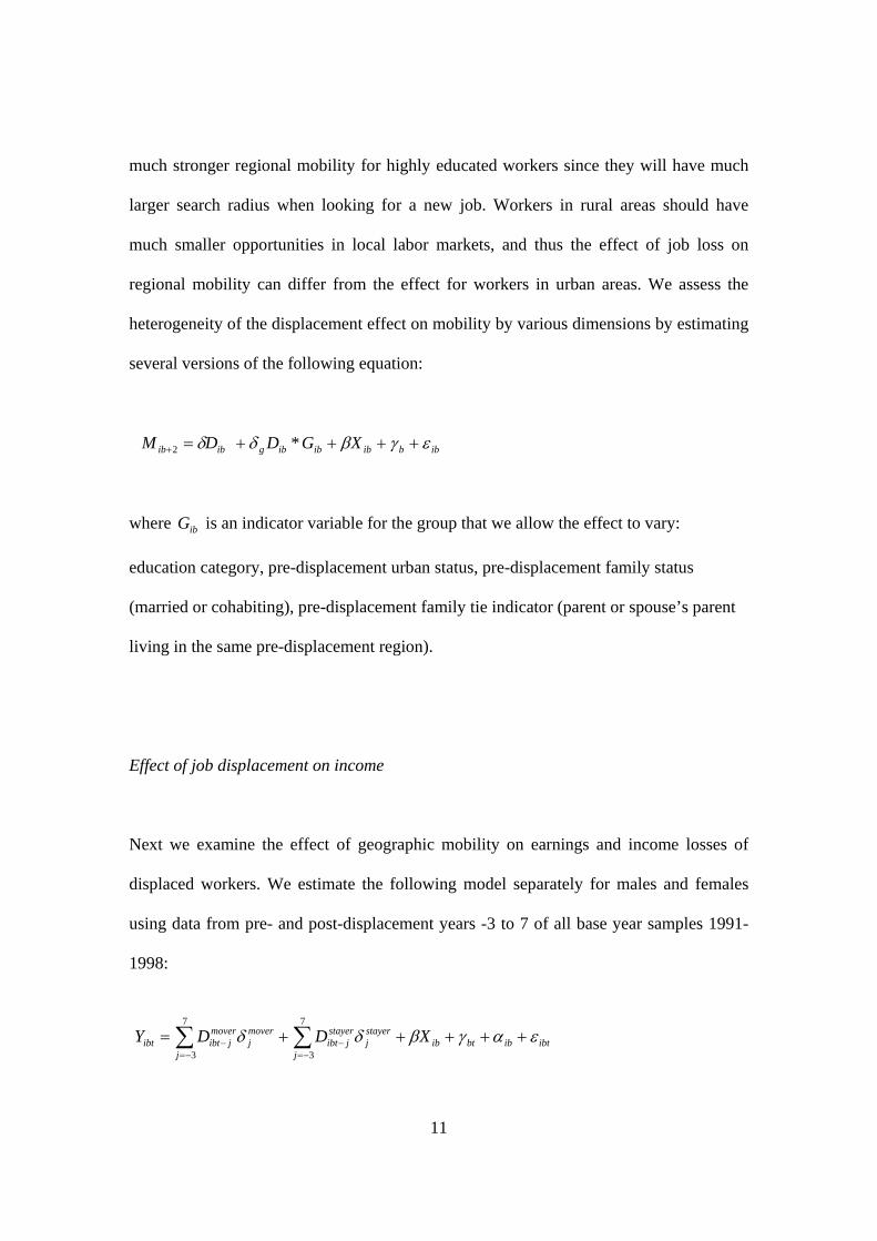
much stronger regional mobility for highly educated workers since they will have much

larger search radius when looking for a new job. Workers in rural areas should have

much smaller opportunities in local labor markets, and thus the effect of job loss on

regional mobility can differ from the effect for workers in urban areas. We assess the

heterogeneity of the displacement effect on mobility by various dimensions by estimating

several versions of the following equation:

where ibG is an indicator variable for the group that we allow the effect to vary:

education category, pre-displacement urban status, pre-displacement family status

(married or cohabiting), pre-displacement family tie indicator (parent or spouse’s parent

living in the same pre-displacement region).

Effect of job displacement on income

Next we examine the effect of geographic mobility on earnings and income losses of

displaced workers. We estimate the following model separately for males and females

using data from pre- and post-displacement years -3 to 7 of all base year samples 1991-

1998:

ibtibbtibj j

stayerj

stayerjibt

moverj

moverjibtibt XDDY

7

3

7

3

ibbibibibgibib XGDDM *2

12

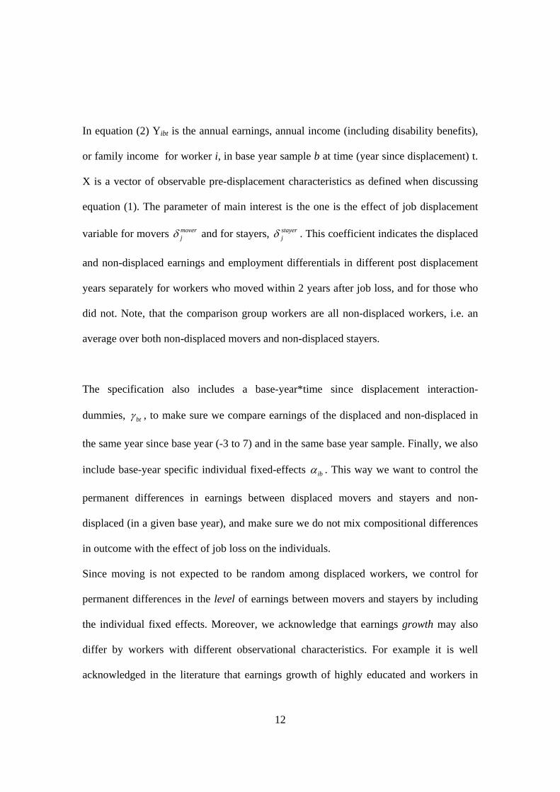
In equation (2) Yibt is the annual earnings, annual income (including disability benefits),

or family income for worker i, in base year sample b at time (year since displacement) t.

X is a vector of observable pre-displacement characteristics as defined when discussing

equation (1). The parameter of main interest is the one is the effect of job displacement

variable for movers moverj and for stayers, stayer

j . This coefficient indicates the displaced

and non-displaced earnings and employment differentials in different post displacement

years separately for workers who moved within 2 years after job loss, and for those who

did not. Note, that the comparison group workers are all non-displaced workers, i.e. an

average over both non-displaced movers and non-displaced stayers.

The specification also includes a base-year*time since displacement interaction-

dummies, bt , to make sure we compare earnings of the displaced and non-displaced in

the same year since base year (-3 to 7) and in the same base year sample. Finally, we also

include base-year specific individual fixed-effects ib . This way we want to control the

permanent differences in earnings between displaced movers and stayers and non-

displaced (in a given base year), and make sure we do not mix compositional differences

in outcome with the effect of job loss on the individuals.

Since moving is not expected to be random among displaced workers, we control for

permanent differences in the level of earnings between movers and stayers by including

the individual fixed effects. Moreover, we acknowledge that earnings growth may also

differ by workers with different observational characteristics. For example it is well

acknowledged in the literature that earnings growth of highly educated and workers in

13

urban areas differs from the earnings growth of less educated workers or workers in rural

areas (Glaeser and Mare, 2001). In order to take this into account we let the age-earnings

profiles differ between workers in urban and rural locations, and for workers in different

education categories. The estimates obtained from this fixed effects approach cannot be

interpreted as the causal effect of mobility, since the (unobservable) factors affecting

selection into migration may also affect earnings growth after job loss. However, we

claim that the set up allows us to provide transparent new evidence on how the income

patterns of job losers depend on their mobility decisions.

In order to understand the mechanism how mobility is related to worker’s post

displacement outcomes, we investigate whether workers who move to a region where

parents are located (back home) have different labor market outcomes than movers for

work-related reasons. In addition, we analyze whether moving to rural and urban areas

make a difference in terms of earnings. The reason for this descriptive exercise is that

quite a few displaced workers leave the labor market and move back to where they

originally came from and where their parents live. There may be many reasons for this;

cheaper housing, stay with parents, wanting to go back where they grew up.

4 Data, Variable Definitions and Sample Construction

The primary data set we are using is the Norwegian Registry Data, a linked

administrative data set that covers the population of Norway. It covers all Norwegian

residents 16--74 years old in the years 1986-2006. It is a collection of different

14

administrative registers such as the education register, family register, the tax and

earnings register, disability pension. A unique person identification code allows

following workers over time. Unique spouse (married/cohabitation) and parent/children

codes exist. Likewise, unique firm and plant codes allow identifying each worker's

employer and examining whether the plant in which the worker is employed is

downsizing or closing down. We also have an identification code for individuals’

municipality of residences for every year. Plant and regional labour market characteristics

such as industry, size and the rate of unemployment are also available.

Employment is measured as months of full-time equivalent employment over the year.4

Earnings are measured as annual taxable income. The included components are regular

labour income, income as self-employed, and benefits received while on sick leave, being

unemployed and on parental leave. In addition, we include annual disability benefits in

order to take into account the income for the group leaving the labor force. Family

income is defined as the sum of the income of worker and her spouse. Regionally

adjusted real income is the annual income deflated using regional price index, which is

primarily based on house price differences across regional labor markets.

The age of the worker is given in the data set. Tenure is measured in years, using the start

date of the employment relationship in a given plant. Education is measured as the

normalized length of the highest attained education and is not survey based but comes

from the education register where each education institution report every year to Statistics

4 We have three categories of working hours and control for part-time employment as follows: Yit = months of employment if a worker is working more than 30 hours a week, Yit = (months of employment) 0,5 if a worker is working 20-29 hours a week and Yit= (months of employment) 0,1 if a worker is working less than 20 hours a week.

15

Norway. Educational attainment is split in three groups; primary secondary and tertiary

education.

The unique spouse codes are used to merge information on spouse’s labour market

situation. In addition we use unique parent codes to attach information on the location of

worker’s parents and siblings each year. We also merge in information on children’s birth

year from population registers. We use this information to calculate the number of school

age children and the number of under school age children parent has each year.

In order to examine the importance of family ties on mobility decision we define

variables describing the location of parents and siblings. Indicator variable for Parents

and sibling living in the labor market region means that worker’s parent or his sibling

lived in the same regional labor market area in the year when observed. Since it is well

established that first-borns are more mobile than younger siblings (Konrad et al. 2002),

we define variable Younger siblings means that worker has at least one younger sibling.

5 Mobility decision

In this section we will first provide descriptive evidence on the migration behavior,

background characteristics and post-displacement outcomes of displaced and non-

displaced workers. Then we present the regression results.

A. Difference between treatment and control groups

16

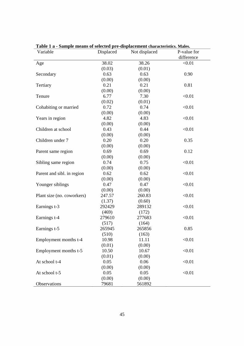
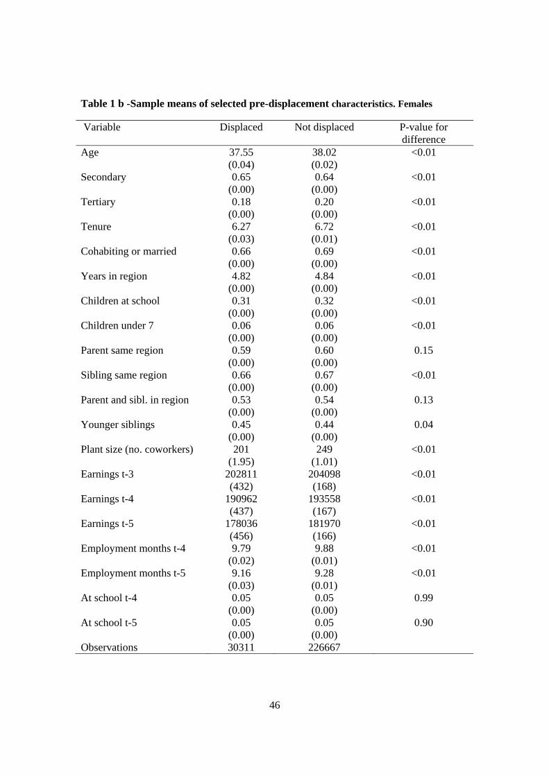
Tables 1a and 1b reports the mean values of the pre-displacement characteristics for

different for displaced and non-displaced workers.5 We present the mean values for

displaced and non-displaced in column one and two, and p-values for testing whether the

means are equal in column three. It is a common finding that displaced and non-displaced

workers tend to have slightly different characteristics in the job displacement literature.

We find the same thing in this case, displaced workers are very similar in terms of

educational attainment, pre-displacement earnings, and the number of children under the

age of seven as well as parental network. On the other hand displaced workers are

slightly older, have higher tenure, a little less likely to be married, and slightly more

unemployed four and five years prior to being displaced. Note that the sample is

constructed to be identical in terms of employment up to three years prior to being

displaced. These are not big differences, however, statistically significant, and thus we

include these controls in the regression analysis, alternatively use them in a pre-stage

using matching.

B. Descriptives: Displacement and mobility

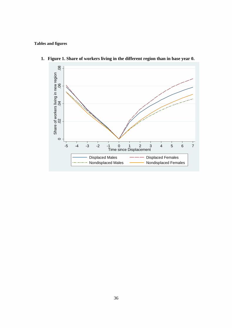
Figure 1 describes the share of movers among displaced and non-displaced workers for

up to seven years following displacement, split by gender. As expected, displaced

workers have a higher probability of moving compared to non-displaced workers in the

years immediately following job loss for both genders. 3.38% of displaced females and

3.02% of displaced males have moved to a new region by the second year after job loss,

5 In the Appendix in Table 1A we split both displaced and non-displaced workers in movers and staying in order to show the difference between the movers and stayers for the treatment and control group. We notice that movers are very similar across the two groups as are stayers.

17

as compared to 2.10% of non-displaced females and 1.97% non-displaced males. Hence

there is about a one percentage point difference for displaced as compared to non-

displaced workers indicating up to about 50% unconditioned increase in the probability

of moving after being displaced which is a big impact. The difference from the first year

following displacement is kept also after 7 years so it appears that it is the first shock of

displacement which is important for moving. This result is consistent with theoretical

predictions. Job loss (personal unemployment) should augment migration likelihood, due

to reduction of present income and, thus, the opportunity costs of moving. Notice also,

that there is a slight mobility difference between those who will be displaced and non-

displaced in the years leading up to displacement, but the difference increases after

displacement.

The figures also indicate that the regional migration mobility in Norway is high. This is

in line with the comparisons undertaken by geographers and economists, where Northern

Europe with Norway is ranked among the countries with the highest regional mobility

rates in Europe (Rees and Kupiszewski, 1999; Rees, Østby, Durham and Kupiszewski,

1999, Machin, Pelkonen, and Salvanes, 2011).

C. Regression results: Displacement, mobility and background factors

Now we turn to results where we condition on all controls within a regression framework.

First we present the results regarding moving decisions; which factors have an impact on

the mobility of displaced and non-displaced workers, and which factors determine some

displaced workers to migrate and some not.

18

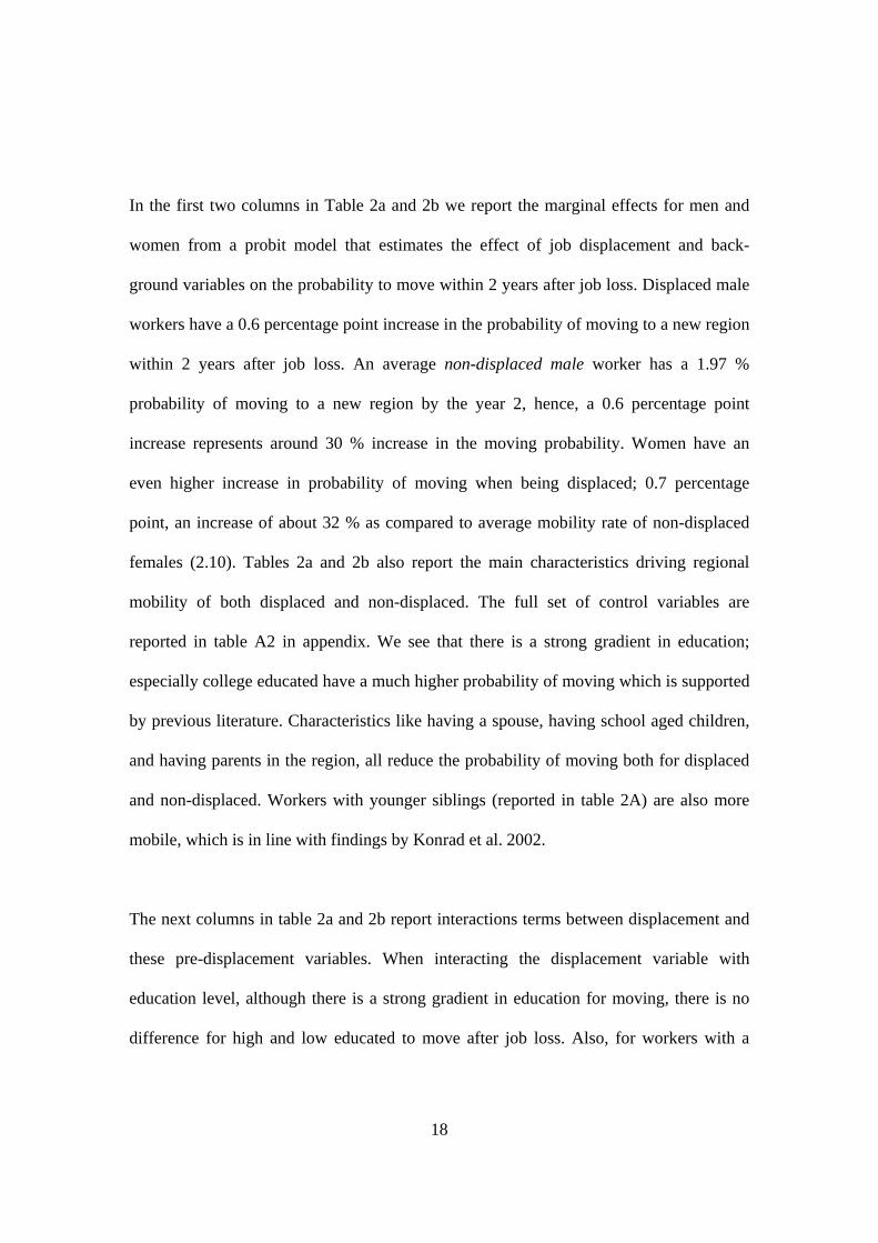
In the first two columns in Table 2a and 2b we report the marginal effects for men and

women from a probit model that estimates the effect of job displacement and back-

ground variables on the probability to move within 2 years after job loss. Displaced male

workers have a 0.6 percentage point increase in the probability of moving to a new region

within 2 years after job loss. An average non-displaced male worker has a 1.97 %

probability of moving to a new region by the year 2, hence, a 0.6 percentage point

increase represents around 30 % increase in the moving probability. Women have an

even higher increase in probability of moving when being displaced; 0.7 percentage

point, an increase of about 32 % as compared to average mobility rate of non-displaced

females (2.10). Tables 2a and 2b also report the main characteristics driving regional

mobility of both displaced and non-displaced. The full set of control variables are

reported in table A2 in appendix. We see that there is a strong gradient in education;

especially college educated have a much higher probability of moving which is supported

by previous literature. Characteristics like having a spouse, having school aged children,

and having parents in the region, all reduce the probability of moving both for displaced

and non-displaced. Workers with younger siblings (reported in table 2A) are also more

mobile, which is in line with findings by Konrad et al. 2002.

The next columns in table 2a and 2b report interactions terms between displacement and

these pre-displacement variables. When interacting the displacement variable with

education level, although there is a strong gradient in education for moving, there is no

difference for high and low educated to move after job loss. Also, for workers with a

19

spouse and with school aged children, there is no difference in displacement effect on

mobility. Interestingly, for men having a family in pre-displacement region significantly

reduces the probability to move after job loss. This indicates that family ties indeed

matter for worker’s mobility decision. This can be explained by various reasons: parents

may help individuals to find new employment in the region, they can provide child care

help or individuals may just prefer being close to the family.

When interacting the displacement variable with urban dummy we find that job

displacement increases mobility more for workers in the rural areas, although the

difference is not statistically significant.6 This may reflect that workers in rural areas

have more limited employment opportunities and thus displaced workers need to search

employment from wider areas. It also indicates that one of the mechanisms for the still

ongoing strong urbanization process in Norway is that workers lose their job and then

move (see Butikofer, Polovkova and Salvanes, 2012, for an analysis of the urbanization

process in Norway).

6. Labor market outcomes for movers and non-movers

Next we investigate how earnings and employment outcomes after job displacement are

related to worker’s mobility decisions.

A. Descriptives: Post-displacement outcomes by displacement and moving status

6 The main effect of living in rural area is negative, indicating that workers in rural areas are less mobile. Since the model includes region fixed effects we could not estimate the main effect of living in rural area. In the model without region fixed effects the coefficient on rural dummy is -0.003.

20

Table 3 provides the employment status in b+2 (short run) and b+7 (long run) by gender,

displacement and moving status. Displaced workers are workers that were displaced

because of plant closure or downsizing between b and b+1. Stayers are workers who live

the same regional labor market in year b+2 as before displacement (year b). Movers have

a new local labor market code by second post displacement year b+2. This information

will be useful when interpreting the regressions results in terms of post displacement

earnings patterns for movers compared to non-movers; they may fare very differently in

the labor market, leaving the labor market, and moving to an area where they have

networks.

From the upper part of the table we see that about 86 percent of the displaced male

workers are reemployed within two years. Displaced male workers who have moved to a

new region have significantly lower re-employment rates (81 percent) than the ones who

have stayed in the region they lived in before being displaced from their jobs (86

percent). Among the non-displaced male workers the stayers also seem to have much

lower employment rates at year t+2 than stayers.

The lower panel reports the results for females. The difference in the employment rate

between movers and stayers seems to be higher than for males. Only around 69% of

displaced female workers who have moved to a new region are working two years after

the job loss, while 82% of displaced stayers are working. When investigating the end-

states in more detail, the table shows that most of the male and female movers that end up

21

being outside labor force live in the regions where either their or their spouse’s parents or

siblings are located.

There may be several explanations why the descriptive evidence indicates that movers do

have worse employment levels than non-movers. First, it may well be that workers move

for non-work related reasons. Table A1 showed that family ties are very important for

workers mobility decisions and that people are generally willing to live close to their

family members. Thus, there may be some workers moving “back home” even though the

employment opportunities in these regions are limited. The fact that the difference

between movers and stayers is especially big for women, may indicate that women are

more likely to be so called “tied movers” and that it is the male in the family whose

employment decisions dominates in families moving decisions.

Another reason for the difference between movers and stayers is that the movers are

negatively selected group. Workers who do not find employment directly after losing

their jobs are more likely to migrate. It may well be that these workers have some

(unobservable) characteristics that are correlated with their lower re-employment

probability.

The short term results carry over to long-term results. Most of the difference in

employment difference between displaced and non-displaced and movers and non-

movers are kept after 7 years. There is a little bit of convergence across groups, but it is

fair to say that the displacement shock appears to make the difference in outcomes in

22

terms of employment. We are looking at un-conditioned rates here so part of the

difference in employment rates between movers and stayers may be due to observable

characteristics.

In order to further investigate the reasons behind the difference in employment rates

between movers and stayers we also split the sample to those who live in urban or rural

location or in a region with family members (not reported here). Workers moving to

urban locations had s higher employment rates than those moving to rural locations (84%

and 78% for males, 74% and 65% for females). Also, workers moving to regions with

family members had lower re-employment regions than workers moving to regions

without family members.

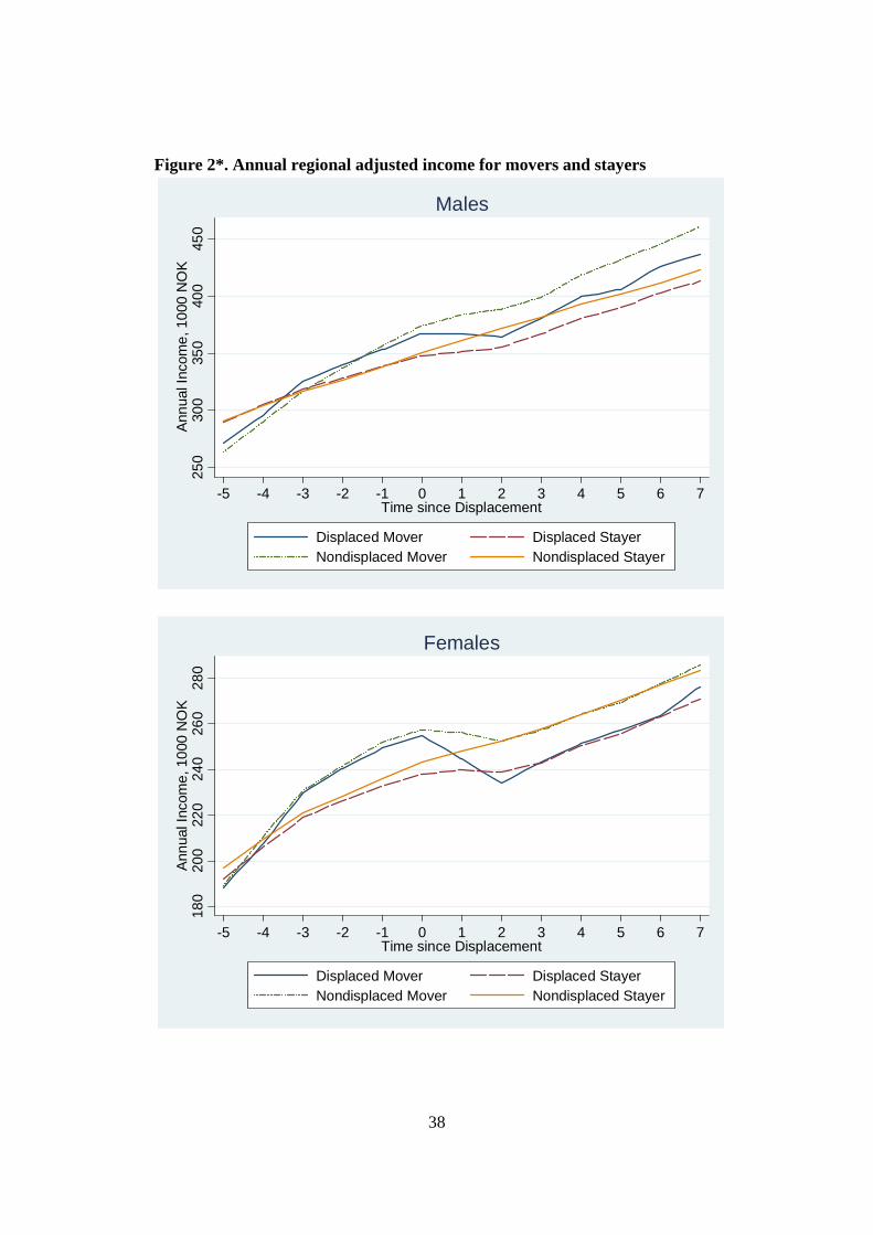
B. Descriptives: Post-displacement income by displacement and moving status

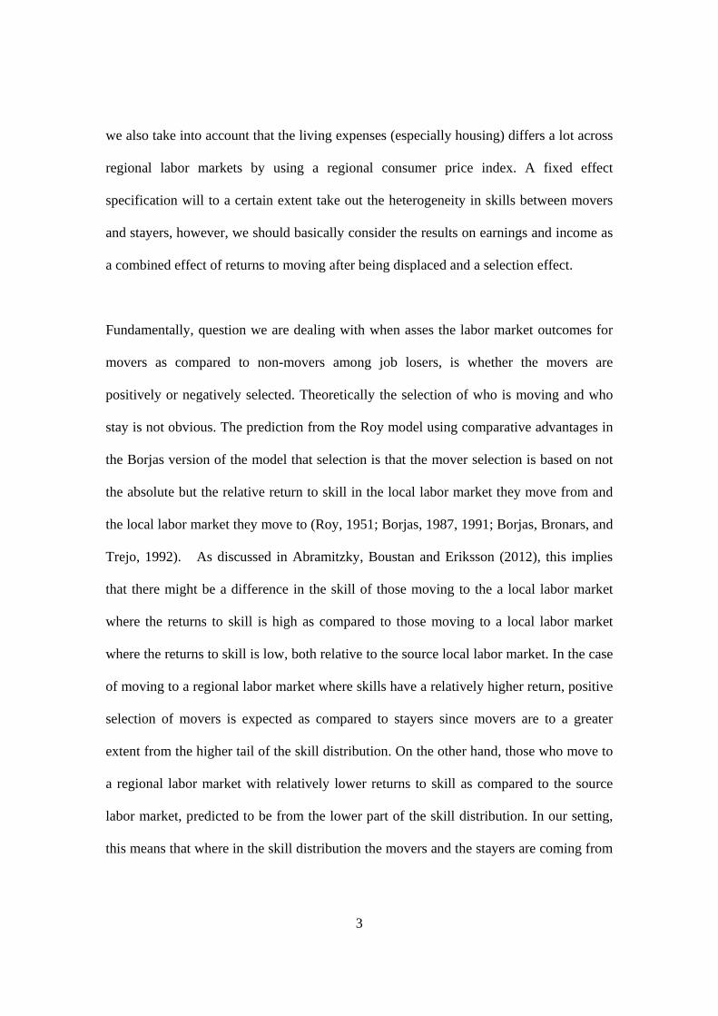
In Figure 2 we present unconditioned mean of average annual income including of

disability benefits (and using a regional CPI) for workers by moving and displacement

status in years before and after job displacement. The results show that the raw pre-

displacement earnings difference between displaced and non-displaced workers is

relatively small. However, there seem to be a large pre-displacement (and pre-move)

difference between movers and stayers. This indicates, as expected that movers tend to be

a selected group, see Table A1 for the unconditioned mean differences.

23

The figure does indicate that job displacement was an exogenous shock to these workers.

Job displacement reduces the earnings of displaced workers and opens up a significant

earnings gap between displaced and non-displaced workers. In line with previous

findings (e.g. Jacobson et al., 1993) the earnings difference between displaced and non-

displaced begins a couple of years before the job loss occurs.

Even though the level of earnings for movers is higher for movers than for stayers, the

drop in earnings after job loss seems to be higher for displaced movers than for displaced

non-movers especially for females. For females, the difference between movers and

stayers is much more pronounced, which indicates that women are more likely to work

for reason that are not due to their own career (tied movers).

C. Fixed effect regression results: Income Loss for Displacement by Migration

Status

Our final aim of the paper is to analyze to what degree the earnings losses found for

workers who lose their jobs are connected to regional mobility. We have already

established that job displacement increases regional mobility, now we want to analyze

within a fixed effects set up whether there are big difference in income effects of job

displacement between movers and stayers. We are using the non-displaced as control

group for both displaced movers and non-movers. We do acknowledge that mobility

decision is highly endogenous so we are cautious not to interpret our estimates as causal

effects of mobility. However, by carefully analyzing the income patterns before and after

24

job loss, we can provide transparent and new information on how earnings losses of

displaced workers are related to their mobility decisions. Since we already have seen that

tied-movers may be an issue, we also provide results for family income.

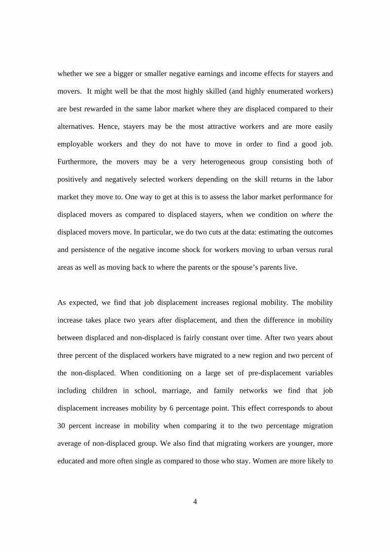
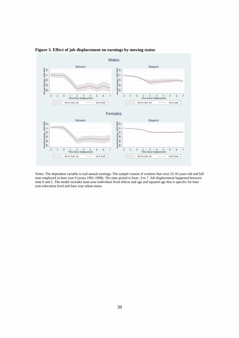
In Figure 3 we present the results of the regression that estimates the effect of job

displacement on annual taxable earnings. Workers with 0 annual earnings are included in

the sample, and thus effect captures both the effect on employment and earnings. The

figure plots the point estimates and confidence intervals of job displacement dummies

separately for movers and stayers. Since model includes fixed effects for each individual

in a given base year sample, we cannot estimate the effect for the first time period -3, and

it is thus used as the base-level. The model also includes base-year specific time dummies

and age and squared age that is specific for base year-education level and base year urban

status.

We observe that before the job loss there was no significant difference in earnings growth

between these groups. After job displacement, earnings drop dramatically for both

movers and stayers. The effect of job displacement on earnings is strongest in the second

post displacement year. The earnings losses for movers are larger than for stayers.

Displaced male movers annual earnings decrease on average 26,500 NOK (the dollar is

about 6 to 1 to the Norwegian kroner (NOK), so that this a little more than 4,000 dollars).

This corresponds to 7.9 % decrease in annual earnings7. For stayers the drop is less

dramatic, displaced workers that have moved to a new region experience a -14,000 NOK

7 As compared to average annual earnings of non-displaced male workers in year 2: 334,196 NOK. The estimated effect of job displacement for male movers in the year 2 is -26,520 . For male stayers the effect is -14,043.

25

drop in earnings (4.2 %). The negative effect of job displacement remains until the 7th

post-displacement year.

For women, the difference in the earnings loss between stayers and movers is even more

pronounced. On the second post displacement year, the earnings drop for displaced

movers is on average -28,800 NOK. This corresponds to a 12.6 % reduction in the mean

earnings8. For displaced female workers who stay in the pre-displacement region the

estimated effect is -8,800 NOK (around 3.8 %). The results are similar when we use as a

dependent variable total income, i.e. annual earnings and disability benefits. These results

are reported in table A1 in Appendix.9

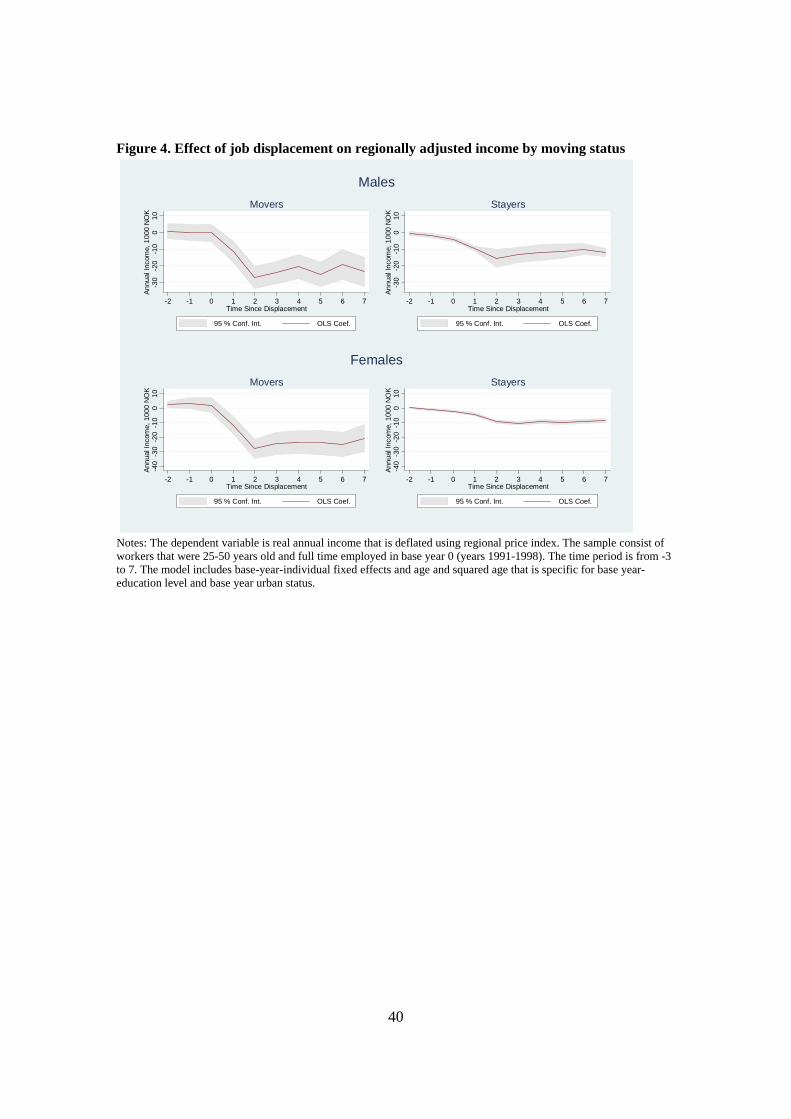
The difference between movers and stayers may also reflect the fact that workers may

move to region with lower living expenses after having lost their jobs. In order to take

this into account we use as a dependent variable regionally adjusted income measure

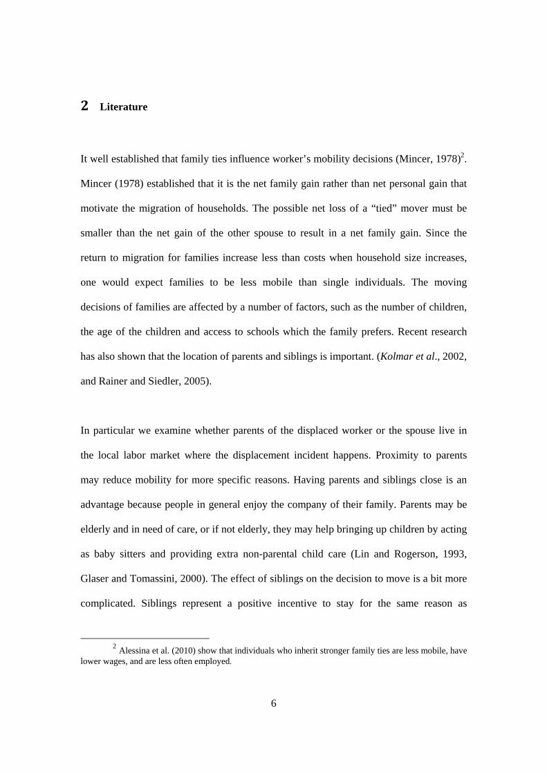
(including disability benefits). Figure 4 reports the estimated effect of job displacement

on regionally adjusted annual income in different time periods since job loss. Again, we

find that movers have larger income losses after job displacement than stayers, although

the difference between movers and stayers diminishes a bit. The drop in annual income in

the second post displacement year for male movers is -26,900 NOK (7.25%) and for male

8 The average annual earnings of non-displaced female workers in year 2, 229,663 NOK. The estimated effect of job displacement for female movers in the year 2 is -26, 908. For female stayers the effect is –8,833. 9 Note, since the number of disability pension recipients is relatively small, the difference in the mean income with and without disability pensions is relatively small. The average annual income (with disability pension) for non-displaced males in year 2 is 334,618 NOK. The estimated effect for movers is -25,685 (-7.67 %).

26

stayers -15,300 NOK (4.12%). For females, the effect for movers is -26,300 NOK (-10.8)

and for stayers -9,519 NOK (-3.76%)10:

It is well established (Mincer, 1978) that it is the net family gain rather than net personal

gain that motivates the migration of households. The possible net loss of a “tied” mover

must be smaller than the net gain of the other spouse to result in a net family gain. In

order to take into account that many of the displaced movers may be so called “tied

movers”, we use as our income measure total family income rather than personal income.

The total family income is created by summing worker’s own and his spouse’s annual

real income. For workers without spouse this equals his own income.

The regression results are presented in Figure 5. We see that job loss has a long-lasting

negative effect on family income.11 Movers suffer bigger earnings losses in the years

immediately following job loss. The drop in year 2 mean family earnings for displaced

male movers is 38,600 NOK that corresponds to 9 % reduction in total family earnings.

For stayers the reduction is smaller, about -14,300 NOK (-3.4%). In time, the earning loss

for movers diminishes. For women, the loss in total family earnings is bigger for movers

in the years immediately following job loss, but the effect fades away in time.

This can reflect both the fact that women are tied movers, and that moving decisions are

also driven by spouse’s employment situation. However, the difference in total family

income between stayers and movers can also reflect the difference in marriage propensity

10 The mean regionally adjusted income for non-displaced males in year 2 is 371,618 and for non-displaced females 252,670 NOK. 11 Results using annual family earnings as dependent variable are reported in figure A2 in appendix.

27

between these two groups. Since movers are younger and less likely to be married as

shown in table 1, the faster growth of family income in later years can also reflect that

they find partner’s in later years. In order to take this into account we restricted the

sample to workers who had a spouse in the base year 0, and investigate how job

displacement affects earnings for stayers and movers. These results are reported in figure

6. Again we find that movers tend to suffer slightly larger losses in total family income

than stayers. The earnings loss in year 2 for displaced male movers is 36,900 NOK

(7.8%) and 13,500 NOK (2.9%) displaced male stayers12. For female movers the drop in

income after job loss is 26,500 NOK (5.6%) and for female stayers 11,800 NOK (2.5 %).

However, the loss fades away in time for women.

D. Heterogeneity in the selection of movers

In order to further examine heterogeneity in selection of movers, we analyzed how the

effect of job displacement varied by the characteristics of the destination where worker

moved to. That is, whether workers moved to urban or rural location, and whether they

moved to regions where their parents or their spouse’s parents locate. We acknowledge

that this analysis is descriptive in nature, since the decision to move to certain kind of

destination is endogenous. We however, believe that by splitting the data to these

subsamples we can provide interesting descriptive information on mobility behavior of

job losers.

12 The average family income for non-displaced males in year 2 is 472 971 NOK.

28

Figure 7 reports the results of fixed-effects regression, where we estimate how income

losses of job losers vary between 4 different categories: 1) workers who stayed in urban

region, 2) workers who moved to urban region, 3) workers who stayed in rural region,

and 4) workers who moved to rural region. The comparison group is all non-displaced

workers, and again we control for worker fixed effects and let the age and age squared

vary by workers pre-displacement urban status and education. The results show that the

negative effect of job displacement for movers is entirely driven by individuals that move

to rural locations. Workers who move to urban regions do not suffer any post-

displacement earnings losses at all, while movers to urban regions suffer severe and long-

lasting earning losses. Stayers in urban and rural locations both suffer some earning

losses after job displacement, but the drop is much smaller than the drop for workers who

move to rural regions.

In order to examine whether family ties are likely to be reason for mobility decision, we

split the sample by parent’s location in year 2. We estimate a similar fixed effect

specification but let the effect of job displacement vary between four categories: 1)

workers who moved (by year 2) to region where her or her spouse’s parent locate, 2)

workers who stayed (until year 2) in pre-displacement region where her or her spouses

parent locate, 3) workers who moved to a region where neither her nor her spouse’s

parent locate and 4) workers who stayed in the region where neither her nor her spouse’s

parent locate. The results are reported in figure 8. The results indicate that workers who

move to a region where family members located suffer bigger earning losses than the

workers who move to regions with no family. Male workers who move to region where

29

their parents do not locate suffer almost no long-term losses. It seems that family ties may

be one reason why workers move to a new region, and these workers tend to have lower

income growth than other displaced workers13.

D. Robustness Checks

Since movers differ from stayers by observational characteristics, as a robustness check,

we trimmed the comparison group by pre-displacement characteristics using an estimated

propensity score. In order to estimate the effect of job displacement for movers we first

estimated a probit model that explained the probability to be “displaced mover” by rich

set of pre-displacement characteristics (reported under figure A4) using data on displaced

movers and all non-displaced workers. We then weighted the non-displaced comparison

group by predicted probability to be “displaced mover”14. This way we made sure that we

compared displaced movers to similar non-displaced workers. In order to estimate the

effect of “job displacement” for stayers, we first estimated the probability to be “a

displaced stayer”, and then we used this predicted probability (propensity score) to

weight the comparison group sample. The results using this approach are reported in

figure A4. The results are relatively similar to unmatched results, for male movers the

effect of job displacement is now smaller.

13 We also examined the heterogeneity of the effect of job displacement by mobility and various

pre-displacement characteristics, including education, urban status and family ties in pre-displacement region. The results by educational categories are reported in appendix. The model is estimated separately for each educational category. The results indicate that movers tend to suffer larger losses than stayers in all educational categories. In absolute terms the earning losses for highly educated are larger, but in percentages the primary educated suffer bigger losses. 14 Following Hirano and Imbens (2001) we estimate the effect of treatment on treated by weigting the data so that the weights equal unity for the treated units and ))(ˆ1/()(ˆ xpxp for the control units, where )(ˆ xp is

the estimated propensity score.

30

6 Concluding remarks

The aim of this paper is to analyze geographic mobility of workers after permanent job

loss, and what influence’s workers decision to move away from region. We provide

evidence that job displacement increases regional mobility, especially for workers whose

parents or siblings do not locate in the region. Family ties are very important for worker’s

mobility decision. Workers are less likely to move away from regions where they parents

or siblings locate, and some move back home after job loss. We also provide descriptive

evidence how earnings losses after job displacement are related to worker’s decision to

migrate from the region. Our findings suggest that workers who move to a new region

after job loss suffer bigger income losses related to stayers. These losses are driven by

workers who move to rural regions and to regions where they have family members.

31

7 Referenses

Alesina, Alberto F. , Yann Algan, Pierre Cahuc and Paola Giuliano, (2010). "Family

Values and the Regulation of Labor," NBER Working Papers 15747, National Bureau of

Economic Research, Inc.

Autor, David H., David Dorn and Gordon H. Hanson, (2013). "The China Syndrome:

Local Labor Market Effects of Import Competition in the United States," Forthcoming

American Economic Review

Boman, Anders (2011). "Does migration pay? Earnings effects of geographic mobility

following job displacement," Journal of Population Economics, Springer, vol. 24(4),

pages 1369-1384, October.

Borjas, George J, (1987). "Self-Selection and the Earnings of Immigrants," American

Economic Review, vol. 77(4), pages 531-53, September.

Borjas, George J. & Bronars, Stephen G. & Trejo, Stephen J., (1992a). "Assimiliation and

Earnings of Young internal Migrants," Review of Economics and Statistics, vol. 74 (1),

pages 170-75.

32

Borjas, George J. & Bronars, Stephen G. & Trejo, Stephen J., (1992b). "Self-selection

and internal migration in the United States," Journal of Urban Economics, vol. 32(2),

pages 159-185, September.

Couch, Kenneth A, and Dana W. Placzek, 2010. "Earnings Losses of Displaced Workers

Revisited," American Economic Review, American Economic Association, vol. 100(1),

pages 572-89, March.

Chiswick, Barry R. (1999). "Are Immigrants Favorably Self-Selected?" The American

Economic Review, Papers and Proceedings. Vol. 89, No. 2, pp. 181-1

Curtis, Simon J., & Warner, John T., (1992): "Matchmaker, Matchmaker: The Effect of

Old Boy Networks on Job Match Quality, Earnings, and Tenure," Journal of Labor

Economics, University of Chicago Press, vol. 10(3), pages 306-30

Eliason, Marcus and Storrie, Donald. (2006), "Lasting or Latent Scars? Swedish

Evidence on the Long-Term Effects of Job Displacement" , Journal of Labor Economics,

volume 24 (2006), pages 831--856

Fallick, Bruce C. (1996): "A Review of the Recent Empirical Literature on Displaced

Workers", Industrial and Labour Relations Review, Vol. 50(1), pp. 5-16

33

Gabriel, Paul E. and Susanne Schmitz, "Favorable Self-Selection and the Internal

Migration of Young White Males in the United States", Journal of Human Resources,

Vol. 30, No. 3 (Summer, 1995), pp. 460-471.

Glaeser, Edward L & Mare, David C, 2001. "Cities and Skills," Journal of Labor

Economics, University of Chicago Press, vol. 19(2), pages 316-42, April.

Greenwood, Michael J. (1997), "The Internal Migration in Developed Countries",

Handbook of Population and Family Economics.

Herz D. E. (1991) Worker Displacement Still Common in the late 1980s, Bulletin 2382,

Bureau of Labour Statistics.

Herzog, Henry W. Alan M. Schlottmann, and Thomas P.Boehm (1993): Migration as

Spatial Job Search: A Survey of Empirical Findings, Regional Studies, Vol. 27, 4,

pp.327-340.

Hirano K., and Imbens, G. (2001): "Estimation of Causal Effects using Propensity Score

Weighting: An Application to Data on Right Heart Catheterization," Health Services and

Outcomes Research Methodology 2: 259-278.

Huttunen, Kristiina, Jarle Møen and Kjell G. Salvanes, (2011). "How Destructive Is

Creative Destruction? Effects Of Job Loss On Job Mobility, Withdrawal And Income,"

34

Journal of the European Economic Association, European Economic Association, vol.

9(5), pages 840-870, October.

Jacobson, Louis S., Robert J. LaLonde and Daniel G. Sullivan (1993): "Earnings Losses

of Displaced Workers", American Economic Review, Vol. 83(4), pp. 685-709

Konrad, Kai A & Künemund, Harald & Lommerud, Kjell Erik & Robledo, Julio R,

(2002): "Geography of the Family", American Economic Review, 92 (4) pp: 981-998

Kramarz, Francis & Nordström Skans, Oskar, (2011). "When strong ties are strong

Networks and youth labor market entry," Working Paper Series, Center for Labor Studies

2011:18, Uppsala University, Department of Economics

Mincer, (1978), "Family Migration Decisions"Journal of Political Economy, Vol. 86 (5)

pp.749-73

Pellizzari, Michele (2004): "Do friends and relatives really help in getting a good job?"

Discussion Paper 623. CEP: London.

Pekkala, Sari and Hannu Tervo (2002), "Unemployed and Migration: Does Moving

Help?", Scandinavian Journal of Economics, Vol. 104 (4)

35

Podgursky, Michael; Swaim, Paul (1993) "Job Displacement and Labor Market Mobility.

Final Report".Massachusetts Univ., Amherst. Dept. of Economics.

Rainer, Helmut and Thomas Siedler (2005): "O Brother, Where Art Thou? The Effects of

Having a Sibling on Geographic Mobility and Labor Market Outcomes", IZA Discussion

paper 1842

Rege, Mari, Kjetil Telle and Mark Votruba, (2009). "The Effect of Plant Downsizing on

Disability Pension Utilization," Journal of the European Economic Association, MIT

Press, vol. 7(4), pages 754-785, 06.

Stevens, Ann Huff (1997): "Persistent Effects of Job Displacement: The Importance of

Multiple Job Losses", Journal of Labor Economics, Vol. 15(1), pp. 165--188.

36

Tables and figures

1. Figure 1. Share of workers living in the different region than in base year 0. 0

.02

.04

.06

.08

Sha

re o

f wor

kers

livi

ng in

ne

w r

egio

n

-5 -4 -3 -2 -1 0 1 2 3 4 5 6 7Time since Displacement

Displaced Males Displaced FemalesNondisplaced Males Nondisplaced Females

37

Figure 2. Annual earnings for movers and stayers

250

300

350

350

400

Ann

ual E

arn

ings

, 10

00

NO

K


Displaced Mover Displaced StayerNondisplaced Mover Nondisplaced Stayer

Males

180

260

240

220

200

Ann

ual E

arn

ings

, 10

00

NO

K



Females

38

Figure 2*. Annual regional adjusted income for movers and stayers

450

400

350

300

250

Ann

ual I

ncom

e, 1

000

NO

K



Males

280

260

240

220

200

180

Ann

ual I

ncom

e, 1

000

NO

K



Females

39

Figure 3. Effect of job displacement on earnings by moving status

-30

-20

-10

01

0A

nn

ual

Ea

rnin

gs,

10

00

NO

K

-2 -1 0 1 2 3 4 5 6 7Time Since Displacement

95 % Conf. Int. OLS Coef.

Movers

-30

-20

-10

01

0A

nn

ual

Ea

rnin

gs,

10

00

NO

K



Stayers

Males

-40

-30

-20

-10

01

0A

nn

ual

Ea

rnin

gs,

10

00

NO

K



Movers-4

0-3

0-2

0-1

00

10

An

nu

al E

arn

ing

s, 1

00

0 N

OK



Stayers

Females

Notes: The dependent variable is real annual earnings. The sample consist of workers that were 25-50 years old and full time employed in base year 0 (years 1991-1998). The time period is from -3 to 7. Job displacement happened between time 0 and 1. The model includes base-year-individual fixed effects and age and squared age that is specific for base year-education level and base year urban status.

40

Figure 4. Effect of job displacement on regionally adjusted income by moving status -3

0-2

0-1

00

10

An

nu

al I

nco

me,

10

00

NO

K



Movers

-30

-20

-10

01

0A

nn

ual

In

com

e, 1

00

0 N

OK



Stayers

Males

-40

-30

-20

-10

01

0A

nn

ual

In

com

e, 1

00

0 N

OK



Movers-4

0-3

0-2

0-1

00

10

An

nu

al I

nco

me,

10

00

NO

K



Stayers

Females

Notes: The dependent variable is real annual income that is deflated using regional price index. The sample consist of workers that were 25-50 years old and full time employed in base year 0 (years 1991-1998). The time period is from -3 to 7. The model includes base-year-individual fixed effects and age and squared age that is specific for base year-education level and base year urban status.

41

Figure 5. Effect of job displacement on family income by moving status (both earnings and income, remove other)

-50

-40

-30

-20

-10

0F

am

ily I

nco

me

, 10

00

NO

K



Movers

-50

-40

-30

-20

-10

0F

am

ily I

nco

me

, 10

00

NO

K



Stayers

Males

-60

-40

-20

02

0F

am

ily I

nco

me

, 10

00

NO

K



Movers-6

0-4

0-2

00

20

Fa

mily

Inc

om

e,

100

0 N

OK



Stayers

Females

Notes: The dependent variable is real annual family income (including disability pension).

42

Figure 6. Effect of job displacement on family income by moving status -5

0-4

0-3

0-2

0-1

00

Fa

mily

Inc

om

e,

100

0 N

OK



Movers

-50

-40

-30

-20

-10

0F

am

ily I

nco

me

, 10

00

NO

K



Stayers

Males

-60

-40

-20

02

04

0F

am

ily I

nco

me

, 10

00

NO

K



Movers-6

0-4

0-2

00

20

40

Fa

mily

Inc

om

e,

100

0 N

OK



Stayers

Females

Notes: The dependent variable is real annual family income (including disability pension). The sample consist of workers that were 25-50 years old and full time employed and who had a spouse in base year 0 (years 1991-1998). The time period is from -3 to 7. Since model includes fixed effects for each individual in a given base year sample, we cannot estimate the effect for the first time period -3, and it is thus used as the base-level. The model also includes base year specific time dummies and age and squared age that is specific for base year-education level and base year urban status (in order to take into account that age-earnings profiles differ between workers from different educational groups and locations).

43

Figure 7. Effect of job displacement by mobility and urban status of location in year t+2

-60

-40

-20

020

Ann

ual

Inco

me,

100

0 N

OK



Movers to Urban Region

-60

-40

-20

020

Ann

ual

Inco

me,

100

0 N

OK



Stayers in Urban Region

-60

-40

-20

020

Ann

ual

Inco

me,

100

0 N

OK



Movers to Rural Region-6

0-4

0-2

00

20A

nnu

al In

com

e, 1

000

NO

K



Stayers in Rural Region

Males

-60

-40

-20

020

Ann

ual

Inco

me,

100

0 N

OK



Movers to Urban Region

-60

-40

-20

020

Ann

ual

Inco

me,

100

0 N

OK



Stayers in Urban Region

-60

-40

-20

020

Ann

ual

Inco

me,

100

0 N

OK



Movers to Rural Region

-60

-40

-20

020

Ann

ual

Inco

me,

100

0 N

OK



Stayers in Rural Region

Females

Notes: The dependent variable is real annual income. FE-model. Family in region means parent of the worker or his spouse is a resident in the same region at year 2., See text under table 4 for details.

44

Figure 8. Effect of job displacement by mobility and family ties in location in year 2 -6

0-4

0-2

00

20A

nnu

al In

com

e, 1

000

NO

K



Movers to Region where Family

-60

-40

-20

020

Ann

ual

Inco

me,

100

0 N

OK



Stayers in Region where Family

-60

-40

-20

020

Ann

ual

Inco

me,

100

0 N

OK



Movers to Region where No Family

-60

-40

-20

020

Ann

ual

Inco

me,

100

0 N

OK



Stayers in Region where No Family

Males

-40

-20

020

Ann

ual

Inco

me,

100

0 N

OK



Movers to Region where Family

-40

-20

020

Ann

ual

Inco

me,

100

0 N

OK



Stayers in Region where Family

-40

-20

020

Ann

ual

Inco

me,

100

0 N

OK



Movers to Region where No Family

-40

-20

020

Ann

ual

Inco

me,

100

0 N

OK



Stayers in Region where No Family

Females

Notes: The dependent variable is real annual income. FE-model. Family in region means parent of the worker or his spouse is a resident in the same region at year 2. See text under table 4 for specification and controls.

45

Table 1 a - Sample means of selected pre-displacement characteristics. Males. Variable Displaced Not displaced P-value for

difference Age 38.02 38.26 <0.01 (0.03) (0.01) Secondary 0.63 0.63 0.90 (0.00) (0.00) Tertiary 0.21 0.21 0.81 (0.00) (0.00) Tenure 6.77 7.30 <0.01 (0.02) (0.01) Cohabiting or married 0.72 0.74 <0.01 (0.00) (0.00) Years in region 4.82 4.83 <0.01 (0.00) (0.00) Children at school 0.43 0.44 <0.01 (0.00) (0.00) Children under 7 0.20 0.20 0.35 (0.00) (0.00) Parent same region 0.69 0.69 0.12 (0.00) (0.00) Sibling same region 0.74 0.75 <0.01 (0.00) (0.00) Parent and sibl. in region 0.62 0.62 <0.01 (0.00) (0.00) Younger siblings 0.47 0.47 <0.01 (0.00) (0.00) Plant size (no. coworkers) 247.57 260.83 <0.01 (1.37) (0.60) Earnings t-3 292429 289132 <0.01 (469) (172) Earnings t-4 279610 277683 <0.01 (517) (164) Earnings t-5 265945 265856 0.85 (510) (163) Employment months t-4 10.98 11.11 <0.01 (0.01) (0.00) Employment months t-5 10.50 10.67 <0.01 (0.01) (0.00) At school t-4 0.05 0.06 <0.01 (0.00) (0.00) At school t-5 0.05 0.05 <0.01 (0.00) (0.00) Observations 79681 561892

46

Table 1 b -Sample means of selected pre-displacement characteristics. Females

Variable Displaced Not displaced P-value for difference

Age 37.55 38.02 <0.01 (0.04) (0.02) Secondary 0.65 0.64 <0.01 (0.00) (0.00) Tertiary 0.18 0.20 <0.01 (0.00) (0.00) Tenure 6.27 6.72 <0.01 (0.03) (0.01) Cohabiting or married 0.66 0.69 <0.01 (0.00) (0.00) Years in region 4.82 4.84 <0.01 (0.00) (0.00) Children at school 0.31 0.32 <0.01 (0.00) (0.00) Children under 7 0.06 0.06 <0.01 (0.00) (0.00) Parent same region 0.59 0.60 0.15 (0.00) (0.00) Sibling same region 0.66 0.67 <0.01 (0.00) (0.00) Parent and sibl. in region 0.53 0.54 0.13 (0.00) (0.00) Younger siblings 0.45 0.44 0.04 (0.00) (0.00) Plant size (no. coworkers) 201 249 <0.01 (1.95) (1.01) Earnings t-3 202811 204098 <0.01 (432) (168) Earnings t-4 190962 193558 <0.01 (437) (167) Earnings t-5 178036 181970 <0.01 (456) (166) Employment months t-4 9.79 9.88 <0.01 (0.02) (0.01) Employment months t-5 9.16 9.28 <0.01 (0.03) (0.01) At school t-4 0.05 0.05 0.99 (0.00) (0.00) At school t-5 0.05 0.05 0.90 (0.00) (0.00) Observations 30311 226667

47

Notes. The probit marginal effects. The sample consists of workers who in year 0 (base years 1991–1998) are aged 25–50, employed in plants private sector plants with at least 10 workers. Displacement happened btw years t and t+1. Controls include also base year, region, and industry dummies.

Table 2a. The effect of displacement on regional mobility by pre-displacement characteristics. Males. Males (1) (2) (3) (4) (5) (6) Displaced 0.006 0.005 0.005 0.007 0.007 0.006 (0.000)** (0.001)** (0.001)** (0.001)** (0.001)** (0.001)** Displaced*Secondary 0.001 (0.001) Displaced*Tertiary 0.002 (0.001) Displaced*Rural 0.001 (0.001) Displaced*Spouse -0.001 (0.001) Displaced*family in region*

-0.002 (0.001)*

Displaced*school age children

0.001 (0.001)

Secondary Edu 0.001 0.001 0.001 0.001 0.001 0.001 (0.000)* (0.000)* (0.000)* (0.000)* (0.000)* (0.000)* Tertiary Edu 0.006 0.006 0.006 0.006 0.006 0.006 (0.001)** (0.001)** (0.001)** (0.001)** (0.001)** (0.001)** Spouse -0.004 -0.004 -0.004 -0.003 -0.004 -0.004 (0.000)** (0.000)** (0.000)** (0.000)** (0.000)** (0.000)** Family in Region* -0.017 -0.017 -0.017 -0.017 -0.016 -0.017 (0.001)** (0.001)** (0.001)** (0.001)** (0.001)** (0.001)** School Age Children -0.002 -0.002 -0.002 -0.002 -0.002 -0.002 (0.000)** (0.000)** (0.000)** (0.000)** (0.000)** (0.000)** Observations 638789 638789 638789 638789 638789 638789 Notes. The probit marginal effects. Dependent variable is an indicator whether worker moved between year t and t+2. The sample consists of workers who in year 0 (base years 1991–1998) are aged 25–50, employed in plants private sector plants with at least 10 workers. Displacement happened btw years t and t+1. *Parent or spouse’s parents in located in the same pre-displacement region.The regressions include all variables listed in table 3??? as additional controls. Since the specification includes baseyear-region fixed effects variable “urban” could not be estimated. In a model without regional fe-effects its coefficient is 0.003 (0.001).

48

Table 2b. The effect of displacement on regional mobility by pre-displacement characteristics. Females. Females (1) (2) (3) (4) (5) (6) Displaced 0.007 0.009 0.006 0.008 0.008 0.006 (0.001)** (0.002)** (0.001)** (0.001)** (0.001)** (0.001)** Displaced*Secondary -0.002 (0.001) Displaced*Tertiary -0.001 (0.002) Displaced*Rural 0.001 (0.001) Displaced*Spouse -0.002 (0.001) Displaced*family in region*

-0.001 (0.001)

Displaced*school age children

0.001 (0.001)

Secondary 0.002 0.002 0.002 0.002 0.002 0.002 (0.001)** (0.001)** (0.001)** (0.001)** (0.001)** (0.001)** Tertiary 0.006 0.006 0.006 0.006 0.006 0.006 (0.001)** (0.001)** (0.001)** (0.001)** (0.001)** (0.001)** Spouse -0.006 -0.006 -0.006 -0.005 -0.006 -0.006 (0.001)** (0.001)** (0.001)** (0.001)** (0.001)** (0.001)** Family in Region* -0.013 -0.013 -0.013 -0.013 -0.013 -0.013 (0.001)** (0.001)** (0.001)** (0.001)** (0.001)** (0.001)** School Age Children -0.005 -0.005 -0.005 -0.005 -0.005 -0.005 (0.000)** (0.000)** (0.000)** (0.000)** (0.000)** (0.001)** Observations 256040 256040 256040 256040 256040 256040 Notes. The probit marginal effects. Dependent variable is an indicator whether worker moved between year t and t+2. The sample consists of workers who in year 0 (base years 1991–1998) are aged 25–50, employed in plants private sector plants with at least 10 workers. Displacement happened btw years t and t+1. *Parent or spouse’s parents in located in the same pre-displacement region.The regressions include all variables listed in table 3??? as additional controls. Since the specification includes baseyear-region fixed effects variable “urban” could not be estimated. In a model without regional fe-effects its coefficient is 0.003 (0.001).

49

Table 3. Employment status at time t+2 and t+7 by displacement and moving status Males Displaced Non-Displaced Two years after Stayers Movers Stayers Movers Employed 86.41 81.46 95.31 86.45 Same plant 4.67 1.85 75.84 33.07 same firm (diff plant) 17.29 13.17 3.54 7.54 same industry (diff firm) 33.42 26.47 5.40 14.67 Diff industry, private sector 28.60 34.61 9.78 27.55 Public sector 2.43 5.37 0.76 3.61 Not-employed 13.59 18.54 4.69 13.55 Unemployed 5.10 8.18 1.30 4.44

Unempl & no family in region* 1.16 3.86 0.26 2.24 Unempl & family in region* 3.94 4.32 1.04 2.20 At school 0.81 0.92 0.29 0.84 Outside 7.69 9.44 3.10 8.27 Outside & no family in region* 1.46 4.24 0.56 3.77 Outside & family in region* 6.22 5.20 2.55 4.50 No. of observations 76,568 2,384 547,447 10,989 Males Displaced Non-Displaced Seven years after Stayers Movers Stayers Movers Employed 86.49 82.02 89.87 85.10 Not-employed 13.51 17.98 10.13 14.90 No. of observations 75,776 2,331 541,534 10,756 Females Displaced Non-Displaced Two years after Stayers Movers Stayers Movers Employed 82.27 68.90 91.92 73.61 Same plant 3.82 0.79 73.98 24.54 same firm (diff plant) 13.14 8.86 2.83 5.91 same industry (diff firm) 32.44 19.98 4.83 13.24 Diff industry, private sector 27.41 29.43 8.70 23.31 Public sector 5.46 9.84 1.58 6.61 Not-employed 17.73 31.10 8.08 26.39 Unemployed 6.08 14.76 1.76 9.78 Unempl & no family in region* 1.62 7.68 0.43 4.31 Unnempl & family in region* 4.46 7.09 1.33 5.47 At school 1.09 2.07 0.47 1.94 Outside 10.57 14.27 5.85 14.67 Outside & no family in region* 2.36 5.81 1.14 6.55 Outside & family in region* 8.21 8.46 4.71 8.13 No. of observations 29,087 1,016 220,826 4,736 Females Displaced Non-Displaced Seven years after Stayers Movers Stayers Movers Employed 81.60 75.62 85.31 77.86 Not-employed 18.40 24.38 14.69 22.14 No. of observations 28,795 1,005 218,910 4,665 *Parent or sibling of worker or parent or sibling of worker’s spouse

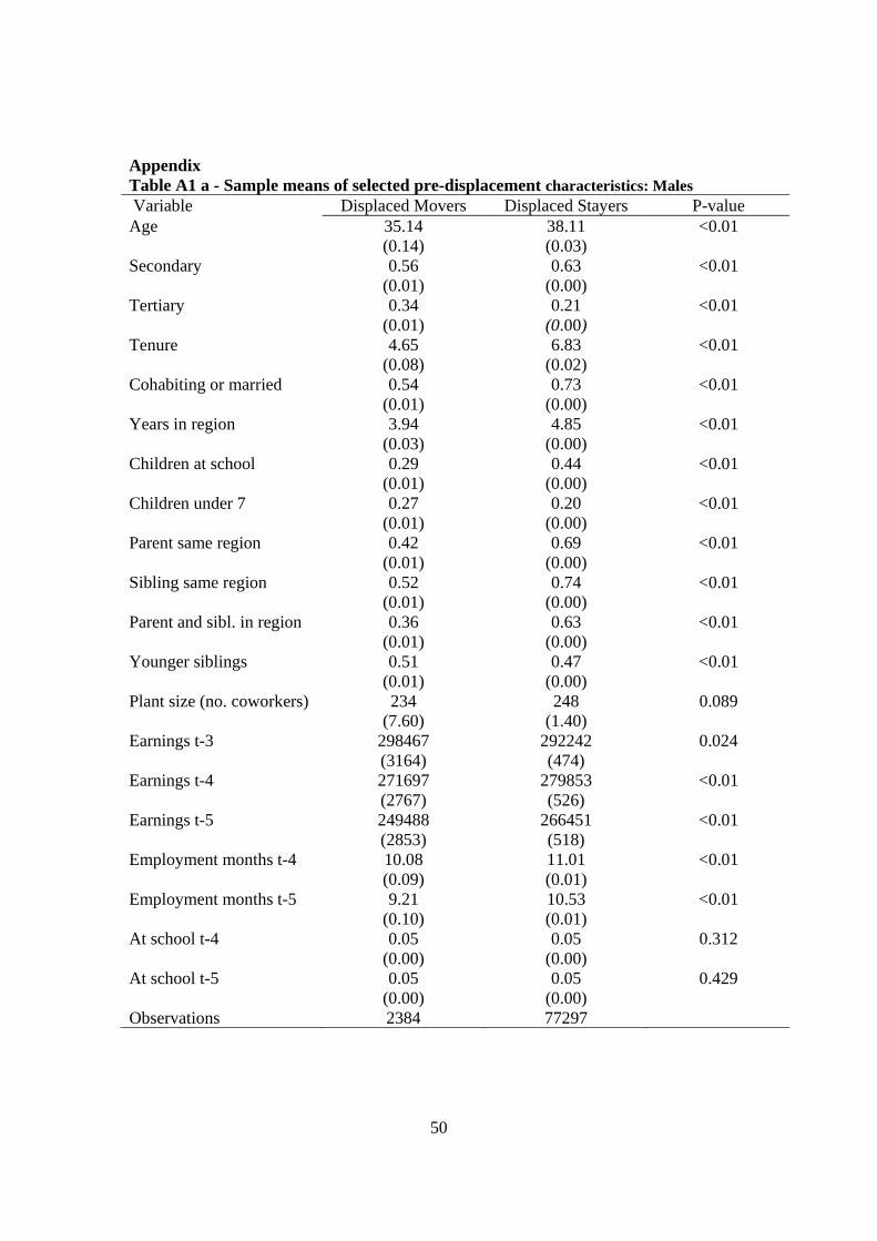
50

Appendix Table A1 a - Sample means of selected pre-displacement characteristics: Males Variable Displaced Movers Displaced Stayers P-value Age 35.14 38.11 <0.01 (0.14) (0.03) Secondary 0.56 0.63 <0.01 (0.01) (0.00) Tertiary 0.34 0.21 <0.01 (0.01) (0.00) Tenure 4.65 6.83 <0.01 (0.08) (0.02) Cohabiting or married 0.54 0.73 <0.01 (0.01) (0.00) Years in region 3.94 4.85 <0.01 (0.03) (0.00) Children at school 0.29 0.44 <0.01 (0.01) (0.00) Children under 7 0.27 0.20 <0.01 (0.01) (0.00) Parent same region 0.42 0.69 <0.01 (0.01) (0.00) Sibling same region 0.52 0.74 <0.01 (0.01) (0.00) Parent and sibl. in region 0.36 0.63 <0.01 (0.01) (0.00) Younger siblings 0.51 0.47 <0.01 (0.01) (0.00) Plant size (no. coworkers) 234 248 0.089 (7.60) (1.40) Earnings t-3 298467 292242 0.024 (3164) (474) Earnings t-4 271697 279853 <0.01 (2767) (526) Earnings t-5 249488 266451 <0.01 (2853) (518) Employment months t-4 10.08 11.01 <0.01 (0.09) (0.01) Employment months t-5 9.21 10.53 <0.01 (0.10) (0.01) At school t-4 0.05 0.05 0.312 (0.00) (0.00) At school t-5 0.05 0.05 0.429 (0.00) (0.00) Observations 2384 77297

51

Table A1 b - Sample means of selected pre-displacement characteristics: Females Variable Displaced Movers Displaced Stayers P-value

Age 33.45 37.69 <0.01 (0.21) (0.04)

Secondary 0.60 0.65 <0.01 (0.02) (0.00)

Tertiary 0.30 0.189 <0.01 (0.01) (0.00)

Tenure 4.62 6.33 <0.01 (0.12) (0.03)

Cohabiting or married 0.40 0.67 <0.01 (0.01) (0.00)

Years in region 3.97 4.85 <0.01 (0.05) (0.00)

Children at school 0.16 0.31 <0.01 (0.01) (0.00)

Children under 7 0.06 0.06 0.707 (0.01) (0.00)

Parent same region 0.39 0.60 <0.01 (0.02) (0.00)

Sibling same region 0.46 0.67 <0.01 (0.02) (0.00)

Parent and sibl. in region 0.33 0.54 <0.01 (0.01) (0.00)

Younger siblings 0.54 0.44 <0.01 (0.02) (0.00)

Plant size (no. coworkers) 206 201 0.658 (10.58) (1.99)

Earnings t-3 212292 202482 <0.01 (2445) (439)

Earnings t-4 192053 190924.1 0.643 (2607) (443)

Earnings t-5 174012 178176 0.101 (2751) (462)

Employment months t-4 9.38 9.80 <0.01 (0.14) (0.02)

Employment months t-5 8.65 9.18 <0.01 (0.16) (0.03)

At school t-4 0.06 0.05 0.782 (0.01) (0.00)

At school t-5 0.05 0.05 0.917 (0.01) (0.00)

Observations 1016 29295

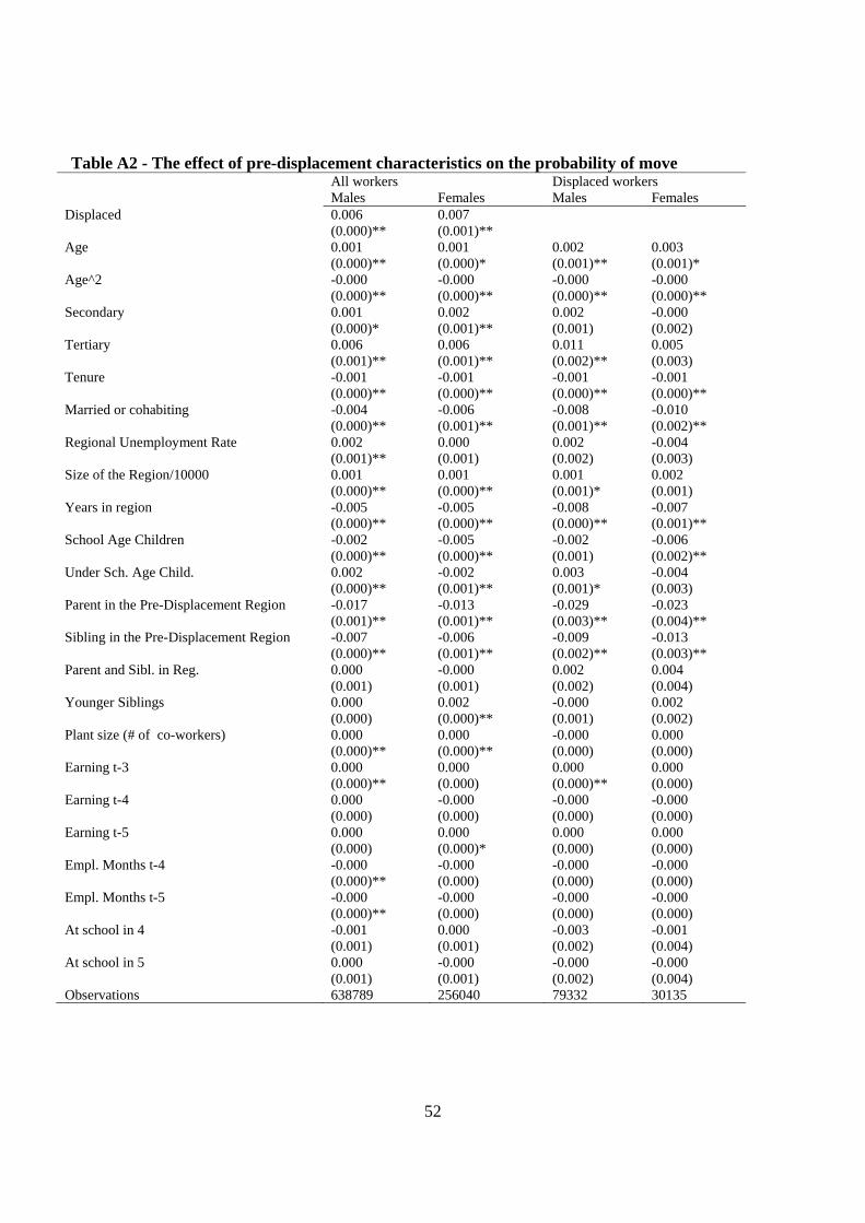
52

Table A2 - The effect of pre-displacement characteristics on the probability of move All workers Displaced workers Males Females Males Females Displaced 0.006 0.007 (0.000)** (0.001)** Age 0.001 0.001 0.002 0.003 (0.000)** (0.000)* (0.001)** (0.001)* Age^2 -0.000 -0.000 -0.000 -0.000 (0.000)** (0.000)** (0.000)** (0.000)** Secondary 0.001 0.002 0.002 -0.000 (0.000)* (0.001)** (0.001) (0.002) Tertiary 0.006 0.006 0.011 0.005 (0.001)** (0.001)** (0.002)** (0.003) Tenure -0.001 -0.001 -0.001 -0.001 (0.000)** (0.000)** (0.000)** (0.000)** Married or cohabiting -0.004 -0.006 -0.008 -0.010 (0.000)** (0.001)** (0.001)** (0.002)** Regional Unemployment Rate 0.002 0.000 0.002 -0.004 (0.001)** (0.001) (0.002) (0.003) Size of the Region/10000 0.001 0.001 0.001 0.002 (0.000)** (0.000)** (0.001)* (0.001) Years in region -0.005 -0.005 -0.008 -0.007 (0.000)** (0.000)** (0.000)** (0.001)** School Age Children -0.002 -0.005 -0.002 -0.006 (0.000)** (0.000)** (0.001) (0.002)** Under Sch. Age Child. 0.002 -0.002 0.003 -0.004 (0.000)** (0.001)** (0.001)* (0.003) Parent in the Pre-Displacement Region -0.017 -0.013 -0.029 -0.023 (0.001)** (0.001)** (0.003)** (0.004)** Sibling in the Pre-Displacement Region -0.007 -0.006 -0.009 -0.013 (0.000)** (0.001)** (0.002)** (0.003)** Parent and Sibl. in Reg. 0.000 -0.000 0.002 0.004 (0.001) (0.001) (0.002) (0.004) Younger Siblings 0.000 0.002 -0.000 0.002 (0.000) (0.000)** (0.001) (0.002) Plant size (# of co-workers) 0.000 0.000 -0.000 0.000 (0.000)** (0.000)** (0.000) (0.000) Earning t-3 0.000 0.000 0.000 0.000 (0.000)** (0.000) (0.000)** (0.000) Earning t-4 0.000 -0.000 -0.000 -0.000 (0.000) (0.000) (0.000) (0.000) Earning t-5 0.000 0.000 0.000 0.000 (0.000) (0.000)* (0.000) (0.000) Empl. Months t-4 -0.000 -0.000 -0.000 -0.000 (0.000)** (0.000) (0.000) (0.000) Empl. Months t-5 -0.000 -0.000 -0.000 -0.000 (0.000)** (0.000) (0.000) (0.000) At school in 4 -0.001 0.000 -0.003 -0.001 (0.001) (0.001) (0.002) (0.004) At school in 5 0.000 -0.000 -0.000 -0.000 (0.001) (0.001) (0.002) (0.004) Observations 638789 256040 79332 30135

53

Figure A1* Effect of job displacement on annual income (including disability benefits) -3

0-2

0-1

00

10

An

nu

al I

nco

me,

10

00

NO

K



Movers

-30

-20

-10

01

0A

nn

ual

In

com

e, 1

00

0 N

OK



Stayers

Males

-30

-20

-10

01

0A

nn

ual

In

com

e, 1

00

0 N

OK



Movers-3

0-2

0-1

00

10

An

nu

al I

nco

me,

10

00

NO

K



Stayers

Females

Notes: The dependent variable is real annual income. Figure A2. Effect of job displacement on real annual family earnings.

-50

-40

-30

-20

-10

0F

am

ily I

nco

me

, 10

00

NO

K



Movers

-50

-40

-30

-20

-10

0F

am

ily I

nco

me

, 10

00

NO

K



Stayers

Males

-60

-40

-20

02

0F

am

ily I

nco

me

, 10

00

NO

K



Movers

-60

-40

-20

02

0F

am

ily I

nco

me

, 10

00

NO

K



Stayers

Females

Notes: The dependent variable is real annual family earnings.

54

Figure A3. Effect of Job Displacement on Earnings: Propensity Score Weighted Regressions

-40

-30

-20

-10

01

0A

nn

ual

Ea

rnin

gs,

10

00

NO

K



Movers

-40

-30

-20

-10

01

0A

nn

ual

Ea

rnin

gs,

10

00

NO

K



Stayers

Males

-40

-30

-20

-10

0A

nn

ual

Ea

rnin

gs,

10

00

NO

K



Movers-4

0-3

0-2

0-1

00

An

nu

al E

arn

ing

s, 1

00

0 N

OK



Stayers

Females

Dependent variable real annual earnings. Propensity score weighted estimation results. Weights equal 1 for treated, and p/(1-p) for non-treated, where p is the estimated propensity score. The pre-displacement (from year 0 if not mentioned otherwise) variable that are used to estimate propensity of treatment (job displacement and move, or job displacement and stay) are age, age squared, secondary, tertiary, base year tenure, married, cohabiting, school age children, children under7, parent same region, spouse’s parent in region, siblings (of the worker or his spouse) in the region, parent and siblings in region, younger siblings, years in region, same region in year t-5, plant size, annual real earnings t-3, annual real earnings t-4, annual real earnings t-5, employment months t-4, employment months t-5, at school t-4, at school t-5, base year dummies, base year region dummies, base year two digit industry dummies. ;

Documents

Job Loss, Family Ties and Regional Mobility