Embed Size (px)
Citation preview
JNABET Journal of the Northeastern Association of Business, Economics and Technology Volume 18 Number 1 Fall 2013 Twitter Effectiveness in Motivating Business Students Melanie O. Anderson Non–Optimal Capital Structure: New Conclusions Using RJR Nabisco LBO Data William H. Carlson and Conway L. Lackman
Ratio Analysis at Private Colleges and Universities in Pennsylvania Michael J. Gallagher The Impact if Increasing and Decreasing Economic Change on the Relevance of Reported Airline Earnings Stephen L. Liedtka and Amy K. Scott From Singular to Global, From Primal to Dual: New Uses for the Herfindahl-Hirschman Index Johnnie B. Linn III Deal Making in Pawn Stars: Testing Theories of Bargaining Bryan C. McCannon and John B. Stevens Food Marketer Web Communication on Palm Oil Sustainability Brenda Ponsford and Thomas Oliver

Journal of the Northeastern Association of Business, Economics, and Technology—Fall 2013 ii
JNABET - Office of the Editor Editor-in-Chief Norman C. Sigmond Kutztown University of Pennsylvania Associate Editor Jerry Belloit Clarion University of Pennsylvania Members of the Executive Board Norman C. Sigmond, Kutztown University of Pennsylvania Chairperson and Editor-in-Chief JNABET M. Arshad Chawdhry, California University of Pennsylvania Treasurer Bradley Barnhorst, DeSales University Secretary Dean F. Frear, Wilkes University NABET President Corina N. Slaff, Misericordia University NABET Vice-President Programs and Conference Chairperson Loreen Powell, Bloomsburg University of Pennsylvania Conference Co-Chairperson Jerry Belloit, Clarion University of Pennsylvania Editor-in-Chief, NABET Conference Proceedings, and Associate Editor JNABET Cori Myers, Lock Haven University of Pennsylvania Co-Editor, NABET Conference Proceedings Board Members-at-Large Marlene Burkhardt, Juniata University Kevin Roth, Clarion University of Pennsylvania Melanie O. Anderson, Slippery Rock University of Pennsylvania
Journal of the Northeastern Association of Business, Economics, and Technology—Fall 2013 iii
Table of Contents
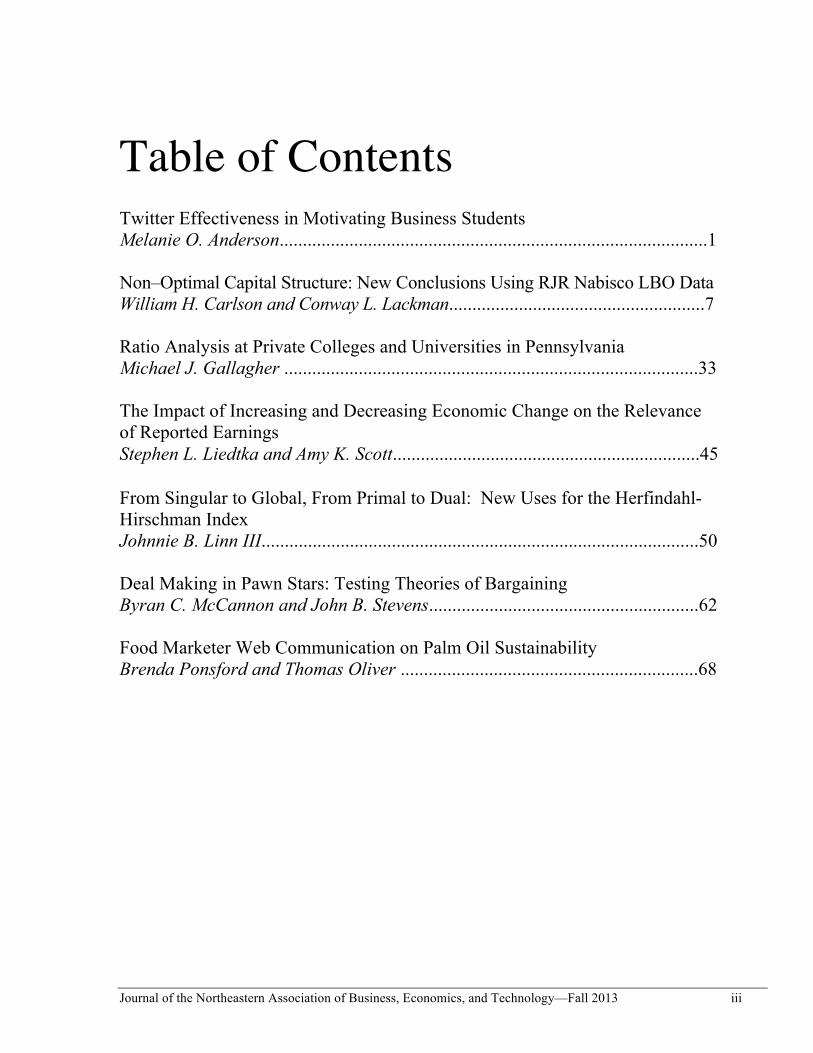
Twitter Effectiveness in Motivating Business Students Melanie O. Anderson............................................................................................1 Non–Optimal Capital Structure: New Conclusions Using RJR Nabisco LBO Data William H. Carlson and Conway L. Lackman.......................................................7 Ratio Analysis at Private Colleges and Universities in Pennsylvania Michael J. Gallagher .........................................................................................33 The Impact of Increasing and Decreasing Economic Change on the Relevance of Reported Earnings Stephen L. Liedtka and Amy K. Scott..................................................................45 From Singular to Global, From Primal to Dual: New Uses for the Herfindahl-Hirschman Index Johnnie B. Linn III..............................................................................................50 Deal Making in Pawn Stars: Testing Theories of Bargaining Byran C. McCannon and John B. Stevens..........................................................62 Food Marketer Web Communication on Palm Oil Sustainability Brenda Ponsford and Thomas Oliver ................................................................68
Journal of the Northeastern Association of Business, Economics, and Technology—Fall 2013 1
TWITTER EFFECTIVENESS IN MOTIVATING BUSINESS STUDENTS
Melanie O. Anderson
ABSTRACT
Universities have selected email as the preferred method to communicate with students, both in using student management systems and course management systems. There is a disconnect between student and university preferences and usage patterns, however, as students view email as outdated. They use social media tools to communicate. This study examines how the use of Twitter, a social media tool limited to 140 character messages, versus the use of email impacted student performance in a managerial accounting course. The instructor taught two different sections of managerial accounting and provided the same information outside of class to students in both courses. In one course, the information was provided via email, and in the second course it was provided via Twitter. Student feedback was sought regarding the use of Twitter and email. Students completed a pre and post quiz and a survey during the course of the term. The instructor compared the average homework scores, the average exam scores, attendance rates, and pre and post quiz results between the two courses to evaluate the use of Twitter versus email.
Keywords: Twitter, Social Media, Micro blogging, Education, Business
INTRODUCTION
Several professors at Harvard, Yale and Columbia have banned laptop use in the classroom (Newsweek, 2008). Other universities, such as UCLA, have installed “kill switches” so that Wi-Fi can be disabled to reconnect students to the classroom and the faculty member (Newsweek, 2008). However, Bill Daggett, CEO of the International Center for Leadership in Education, indicates that education is out of step with students (Daggett, 2010). Modern students are well connected with technology device such as laptops, smart phones, IPods, IPads, outside of school. When all of their connections must be shut down during school, schools appear to be museums to students, according to Daggett.
There are faculty who argue that education should embrace technology. Some argue that dedicated computer labs should be a thing of the past and students should be encouraged to BYOD (Bring Your Own Device) (Baluja, 2011). In fact, “mobile learning devices” may be the new name for the previously banned cell phones in schools (Toppo, 2011). These devices that students have available may represent an opportunity for educators to utilize these tools both in and outside of the classroom.
The traditional method to communicate with college students regarding a course has been with course management systems such as Blackboard and Desire to Learn (D2L) and via campus supported email. However, college students view email as an
“old person’s medium”. (Stebbins, 2007). Students rarely check their email unless their box is full, and then they often delete all emails without reading any of the mail.
This study analyzed an alternative way to use technology tools to achieve a better balance between traditional pedagogy, technology, and student abilities and interests. A relatively new micro blogging social media tool, Twitter, was used instead of email to connect with students outside of class time regarding the course.
BACKGROUND AND LITERATURE REVIEW
Social networking is an important part of college students’ lives; 85% of students at a large research university had Facebook accounts (Mastrodicasa and Kepic, 2005). Twitter is a free social networking tool and the one of the best-known micro blogging services available. It was developed in 2007 to let users share their status. Micro blogging is defined as “a weblog that is restricted to 140 characters per post but is enhanced with social networking facilities” (McFedries, 2007). Educators may be more willing to integrate Twitter into the learning process, as a micro blogging platform is conducive to sharing written information.
Micro blogs platforms have become more powerful due to their mobility; they can be read from mobile phones using short message service or SMS. Twitter is the SMS of the Internet. Twitter users can
Journal of the Northeastern Association of Business, Economics, and Technology—Fall 2013 2
send and read “tweets” of up to 140 characters. Twitter had 300 million users in 2011, and 300 million tweets and 1.6 billion search queries were handled per day (Twitter, 2011). A 2011 Pew Study found that 13 percent of online adults use Twitter, up from 8 percent in 2010 (Smith, 2011). Among 18 to 24 year olds, Twitter usage was 18 percent. The study also noted that 54 percent of these Twitter users access the service using their mobile phones.
Students have access to Twitter readily and continuously. Student smart phone usage is almost ubiquitous; a Pew study indicated that 83% of the U.S. population has a mobile phone and 35% of these phones are smart phones (Pew, 2011). Even if students do not have a smart phone or Twitter account, they can follow a Twitter feed via SMS messaging on their cell phone.
A study in 2007 summarized the uses of micro blogging into three categories: information sharing, information seeking, and friendship-wide relationships (Java, Song, Finin, and Tseng, 2007). Using Twitter in educational settings would be a good fit for information sharing and information seeking. Instructors may be concerned that students may view educational uses of Twitter as unacceptable, or crossing a boundary in social media. A 2009 report on Web 2.0 technologies summarized key findings; one of these was that there are boundaries in web space; personal space, group space, and publishing space. The report allowed that there is room in the so-called group space for teaching and learning (Hughes, 2009).
Other arguments against the use of Twitter are that it is only 140 characters, and it seems like it is a series of individual comments. However, Clive Thomspon notes that Twitter’s effect is cumulative and lets the group using it know more about each other, and become more cohesive and engaged (Thompson, 2007). Ebner, et al.’s research indicated that the use of Twitter or a micro blogging tool can foster process-oriented learning in that it allows continuous and transparent communication between students and lecturers. The researchers further stated that because of the openness of the tool, internal communication would increase. The researchers were also interested in how the use of Twitter impacted informal learning, which can take place in formal learning environments. Informal learning is not directly impacted by the media used, but by the modality of the media. Students were encouraged to “just use the tool to document your learning activities and monitoring your personal learning process”. Students created an average of 7.5 Tweets a day. The researchers concluded that the potential for micro blogging in expanding teaching and learning beyond the classroom is substantial (Ebner, et al, 2010).
As often happens with products, the products are used in ways the designers did not envision. Users use Twitter to post updates on what they are doing or thinking at the moment – similar to Facebook posts. Twitter can also be used to publish information or commentary on particular topics. One of the first uses of Twitter was to report live on sessions during a conference. Subsequent study of this conference use of Twitter was completed by Reinhardt, Ebner, Beham, and Chosta in 2009. Reporting by conference attendees’ concurrently while attending sessions, and comments made before and after a conference, have been labeled the “backchannel”. Using Twitter outside of class can create a course “backchannel”.
Dave Perry has many suggestions for using Twitter in education including creating class chatter outside of class; enhancing the classroom community; getting a sense of the world; tracking a word or idea; tracking a conference; getting instant feedback; following a professional or famous person; improving students’ grammar; honing students’ writing skills; maximizing the teachable moment, using it as a public note pad, and facilitating writing assignments (Perry, 2008).
Twitter can be used by instructors to remind students of homework with daily messages. Twitter can also be used to facilitate homework. At the University of Calgary, English professor Michael Ullyot had his students respond to their Shakespeare texts with tweets. Professor Ullyot watched his hash tag (#engl205) to monitor trending Twitter topics among his students (Baluja, 2011). Twitter can also be used to encourage students to interact with each other using hash tags. Hash tags are words marked with a # symbol that mark keywords or topics in Twitter; Twitter uses this as a way to categorize messages (Twitter, 2011).
The purpose of this study was to analyze the effectiveness and review the student feedback that resulted from the use of Twitter versus email in a managerial accounting course. The instructor taught two different sections of managerial accounting and provided the same information to students in both courses outside of class. In one course, the information was provided via e-mail, and in the second course was provided via Twitter. Students in the second course were asked to follow the faculty member’s Twitter account. Student feedback was sought regarding the use of Twitter and email. Students completed a pre quiz, post quiz and a survey during the course of the term. The instructor compared the average homework scores, the average exam scores, attendance rates, and pre and post quiz results between the two courses. Student feedback was also reviewed and reported.
Journal of the Northeastern Association of Business, Economics, and Technology—Fall 2013 3
METHOLOGY AND HYPOTHESIS
Students no longer use email on a regular basis. This study reviewed the use of Twitter as another avenue of communicating with students, and determined the impact of the use of this tool on student performance. Students had the opportunity to learn using their own cutting-edge mobile devices with which they are enamored. Those students who did not have Wi-Fi access could the proposed social media tool, Twitter, by traditional Internet connections.
The hypothesis was that the application of social media as a primary source of communicating assignment and other key information of the course would enhance student learning. The study compared how this interaction impacted student attendance, homework completion, exam scores, and pre/post test results.
The following five research questions were addressed: Q1: Is there a difference between the use of Twitter or email and student pre and post quiz test scores? Q2: Is there a difference between the use of Twitter or email and student’s class attendance? Q3: Is there a difference between the use of Twitter or email and student’s average homework scores? Q4: Is there a difference between the use of Twitter or email and student’s completion of homework? Q5: Is there a difference between the use of Twitter or email and student exam scores?
The instructor set up a separate Twitter account to
be used as a faculty member; tweets from the account related to coursework only. Tweets were sent Monday through Friday and reminded students of homework, reading and other assignments; directed students to related articles or websites to review for class; and asked students questions related to course material. Students were asked to complete an informed consent document prior to the research study. The two classes met back to back on a MWF afternoon schedule; the first section included out of class communications via Twitter and the second section included out of class communications using email. The instructor sent an average of 2 tweets a day for a 10-week period and an average of one email to every 3 tweets. (The first three weeks of class were not included in the study). All of the tweets were copied to emails so that both sections received the same communications, although several tweets were combined in one email.
Students could set up a Twitter account for free if they did not have one, or they could follow the course without a Twitter account by using SMS and texting
“follow @(instructor name)” to 40404. The instructor would then receive and approve a request for the student to follow the Twitter feed.
This study may benefit future instructors by examining the benefits of using Twitter to communicate with students outside of class.
RESULTS
The study population was students in two
managerial accounting course sections at a state university with a total enrollment of 9,000 students. The two sections involved 71 students (36 in one section and 35 in another) in the Spring 2012 term. Students were asked to complete the pre and post quiz at the beginning and end of the term, as well as the survey document at the end of the term. Descriptive statistical methods (mean, standard deviation, percentage, and frequency) and inferential statistics, specifically the t-Test for the significance of the difference between the means of two independent samples, were used to analyze the results of the data collected including attendance information, homework scores, exam scores and survey data. After the term was complete, the instructor compared attendance, homework scores, and exam scores between the section where Twitter was used and the section where email was used.
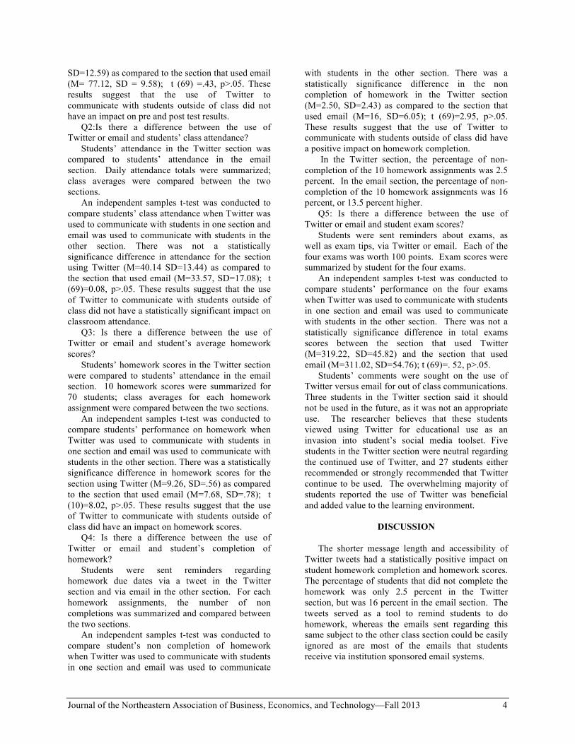
Table 1 Study Results
Q1: Is there a difference between the use of Twitter or email and student pre and post quiz test scores?
Students completed a pre test of seven questions at the beginning of the term and a post test of the same questions at the end of the term. The difference between the pre and post test for each student were summarized and compared between the section that used Twitter and the section that used email to communicate with students.
An independent samples t-test was conducted to compare students’ performance on pre and post tests when Twitter was used to communicate with students in one section and email was used to communicate with students in the other section. There was not a statistically significance difference in the pre and post test scores in the section using Twitter (M=82.47,
Mean Standard Deviation
t-Test
Twitter Email Twitter Email Q1 82.47 77.12 12.59 9.58 .43 Q2 40.14 33.57 13.44 17.08 .08 Q3 9.26 7.68 .56 .78 8.02 Q4 2.50 16 2.43 6.05 2.95 Q5 319.22 311.02 45.82 54.76 .52
Journal of the Northeastern Association of Business, Economics, and Technology—Fall 2013 4
SD=12.59) as compared to the section that used email (M= 77.12, SD = 9.58); t (69) =.43, p>.05. These results suggest that the use of Twitter to communicate with students outside of class did not have an impact on pre and post test results.
Q2:Is there a difference between the use of Twitter or email and students’ class attendance?
Students’ attendance in the Twitter section was compared to students’ attendance in the email section. Daily attendance totals were summarized; class averages were compared between the two sections.
An independent samples t-test was conducted to compare students’ class attendance when Twitter was used to communicate with students in one section and email was used to communicate with students in the other section. There was not a statistically significance difference in attendance for the section using Twitter (M=40.14 SD=13.44) as compared to the section that used email (M=33.57, SD=17.08); t (69)=0.08, p>.05. These results suggest that the use of Twitter to communicate with students outside of class did not have a statistically significant impact on classroom attendance.
Q3: Is there a difference between the use of Twitter or email and student’s average homework scores?
Students’ homework scores in the Twitter section were compared to students’ attendance in the email section. 10 homework scores were summarized for 70 students; class averages for each homework assignment were compared between the two sections.
An independent samples t-test was conducted to compare students’ performance on homework when Twitter was used to communicate with students in one section and email was used to communicate with students in the other section. There was a statistically significance difference in homework scores for the section using Twitter (M=9.26, SD=.56) as compared to the section that used email (M=7.68, SD=.78); t (10)=8.02, p>.05. These results suggest that the use of Twitter to communicate with students outside of class did have an impact on homework scores.
Q4: Is there a difference between the use of Twitter or email and student’s completion of homework?
Students were sent reminders regarding homework due dates via a tweet in the Twitter section and via email in the other section. For each homework assignments, the number of non completions was summarized and compared between the two sections.
An independent samples t-test was conducted to compare student’s non completion of homework when Twitter was used to communicate with students in one section and email was used to communicate
with students in the other section. There was a statistically significance difference in the non completion of homework in the Twitter section (M=2.50, SD=2.43) as compared to the section that used email (M=16, SD=6.05); t (69)=2.95, p>.05. These results suggest that the use of Twitter to communicate with students outside of class did have a positive impact on homework completion.
In the Twitter section, the percentage of non-completion of the 10 homework assignments was 2.5 percent. In the email section, the percentage of non-completion of the 10 homework assignments was 16 percent, or 13.5 percent higher.
Q5: Is there a difference between the use of Twitter or email and student exam scores?
Students were sent reminders about exams, as well as exam tips, via Twitter or email. Each of the four exams was worth 100 points. Exam scores were summarized by student for the four exams.
An independent samples t-test was conducted to compare students’ performance on the four exams when Twitter was used to communicate with students in one section and email was used to communicate with students in the other section. There was not a statistically significance difference in total exams scores between the section that used Twitter (M=319.22, SD=45.82) and the section that used email (M=311.02, SD=54.76); t (69)=. 52, p>.05.
Students’ comments were sought on the use of Twitter versus email for out of class communications. Three students in the Twitter section said it should not be used in the future, as it was not an appropriate use. The researcher believes that these students viewed using Twitter for educational use as an invasion into student’s social media toolset. Five students in the Twitter section were neutral regarding the continued use of Twitter, and 27 students either recommended or strongly recommended that Twitter continue to be used. The overwhelming majority of students reported the use of Twitter was beneficial and added value to the learning environment.
DISCUSSION
The shorter message length and accessibility of
Twitter tweets had a statistically positive impact on student homework completion and homework scores. The percentage of students that did not complete the homework was only 2.5 percent in the Twitter section, but was 16 percent in the email section. The tweets served as a tool to remind students to do homework, whereas the emails sent regarding this same subject to the other class section could be easily ignored as are most of the emails that students receive via institution sponsored email systems.
Journal of the Northeastern Association of Business, Economics, and Technology—Fall 2013 5
Homework scores were 1.58 points or 15.8 percent higher in the section that received tweeted reminders regarding homework due dates. Students were able to tweet the instructor, and each other, with questions about the homework. The availability of this medium without barriers such as passwords, and students’ affinity for this social media tool, made it a preferred method of communication regarding homework questions.
Student class attendance, although not statistically significant, was improved by 13 percent in the section using Twitter. One possible explanation for this improved attendance is a type of Hawthorne effect first reported in business; students being studied and receiving the daily tweets felt special and were motivated by this attention. The students receiving the messages via email did not have the same reaction, as email is not as immediate and is a routine process that all students are used to and can effectively tune out.
There may be a cumulative impact for students in the Twitter section; their class attendance was better and their homework completion and homework scores were higher.
Student performance on exams was not statistically significant between the two sections. Students received tweets reminding them of exam dates and sample questions. Additional research is needed to determine if Twitter’s immediacy and the lack of barriers between tweets and the students positively impacts student performance on exams.
Limitations of this study include the possible impact of other factors on student performance that were not accounted for in the study.
This study provided evidence that timely completion of homework and homework scores were positively impacted by the use of Twitter. Instructors who read this study may question the practicality of using Twitter in the classroom. Several items impact the practicality of using Twitter, including; 1) The instructor’s skill with technology and social media tools; 2) the time the instructor is willing to commit to communicating with students via tweets; and 3) the course material and its applicability to using social media.
The first and most important item is the instructor’s familiarity with technology; including texting, cell phones, smart phones, and the use of social media tools, specifically Twitter. The use of Twitter in this study required basic technology skills and a basic understanding of and experience in using Twitter. This includes the setup of a Twitter account, practice with sending tweets, accepting followers, and explaining to others how use Twitter. If the instructor has teenage children, they can easily help the instructor get up to speed in a few hours.
The instructor’s time investment in using Twitter as an avenue to communicate with students is not extensive, but must be maintained on a regular basis. Twitter’s availability and omnipresence via smart phones allows interactions to go beyond the classroom. It is easy for students to contact and communicate with the instructor via tweets; this may seem to be a large commitment of the instructor’s time. Rather than be chained to Twitter, sending class tweets and handling incoming tweets or hash tag questions can be limited to one or two times a day. This is a similar solution to handling other technology efficiently, such as email, by checking it at regular times rather than continuously.
The final practical item to consider is the applicability of the course material to the use of Twitter and tweets. The very nature of Twitter, using 140 character messages, makes communication brief and to the point. This may seem to be too limited for educational purposes, but the tweets sent have a cumulative impact. Twitter also allows for the customization of learning depending on the student’s needs. Suggestions for the educational use of Twitter include: setup custom classroom hash tags around lessons and topics; Twitter recaps and quizzes of class topics; follow authors and exchange micro reviews of their work; use Twitter as a bulletin board for class; role play via tweets; and, create class newspapers with Twitter streams (Basu, 2013).
CONCLUSIONS AND FUTURE DIRECTION
Overall, student performance increased on homework and homework completion in the managerial accounting course section that used Twitter for out of class communications as compared to the managerial accounting section that used email. The student performance factors reviewed included pre and post test results, class attendance, homework completion, homework scores, and exam scores.
The researcher plans to continue to use Twitter in class and will extend the evaluation of the success of using this social media tool.
The ideas shared in this paper may help other educators in achieving their course objectives by using technology and mobile devices that students have available and are excited to use.
REFERENCES
Baluja, T. (2011, November). Classroom evolution:
current education trends range from the exciting to the divisive and even the bizarre – robot teachers, anybody? The Globe and Mail.

Journal of the Northeastern Association of Business, Economics, and Technology—Fall 2013 6
Basu, S. (2013, April 15). 10 amazing ways for teachers and tutors to use twitter in education. Retrieved July 10, 2013 from http://www.makeuseof.com/tag/10-ways-to-use-twitter-in-education/
Daggett, Bill. (2010). International Center for
Leadership Education. Retrieved December 15, 2010 from http://www.leadered.com/about.html.
Dunlap, J. C., & Lowenthal, P. R. (2009). Tweeting
the night away: Using Twitter to enhance social presence. Journal of Information Systems Education, 20(2).
Ebner, M., Lienhardt, C., Rohs, M., and Meyer, I.
(2010). Micro blogs in higher Education – A chance to facilitate informal and process-oriented learning? Computers and Education, 55, p. 92 – 100.
Hughes, A. (2009). Higher education in a Web 2.0
world. Joint Information Systems Committee (JISC) report. Retrieved January 17, 2012 from http://www.jisc.ac.uk/media/documents/publications/heweb20rptv1.pdf.
Kearns, L.R. & Frey, B. A. (2010 July/August).
Web 2.0 technologies and back channel communications in online learning communities. TechTrends, 54, 4; p. 41 – 50.
Java, A., Song, X., Finin, T., & Tseng, B. (2007).
Why we twitter: Understanding micro-blogging usage and communities. Paper presented at the proceedings of the 9th WebKDD and 1st SNA-KDD 2007 workshop on web mining and social network analysis.
Mandernach, B.J. & Hackathorn, J. (2010,
December). Embracing texting during class. The Teaching Professor, 24, 10; p. 1 – 6.
McFredries, P. (2007). All a-twitter, IEE spectrum,
p. 84. Newsweek (2008, May 10). The laptop gets booted.
Newsweek. Retrieved December 1, 2010 from
http://www.newsweek.com/2008/05/10/the-laptop-gets-booted.html.
Perry, D. (2008). Twitter for Academia. Retrieved
January 17, 2012 from http://academhack.outsidethetext.com/home/2008/twitter-for-academia/.
Pew (2011). Gadget ownership over time. Retrieved
December 8, 2011 from http://www.pewinternet.org/Static-Pages/Trend-Data/Device-Ownership.aspx.
Reinhardt, W., Ebner, M., Beham, G., Costa, C.
(2009). How people are using Twitter during conferences. In V. Hornung-Prähauser, M. Luckmann (Eds.), 5th EduMedia conference (pp. 145–156), Salzburg.
Smith, A. (2011). 13 % of all online adults use
Twitter. Pew Research Center, Washington, DC. Stebbins, L. (2007). Email is evolving – are you?
Searcher: the magazine for database professionals, 15, 2: p. 8 – 12.
Thompson, C. (2008, June 26). Clive Thompson on
how twitter creates a social sixth sense. Wired Magazine, 15.07. Retrieved from January 16, 2012 from http://www.wired.com/techbiz/media/magazine/15-07/st_thompson.
Toppo, G. (2011, July 25). Making students iterate in
digital age; Some consider social media an important tool in the classroom. USA Today, p. 2A.
Twitter (2011). Your world, more connected.
Retrieved January 16, 2012 from http://blog.twitter.com/2011/08/your-world-more-connected.html.
Zhao, D. & Rosson, M.B. (2009). How and why
people Twitter: The role that micro-blogging plays in informal communication at work. In Proceedings of the ACM 2009 international conference on supporting group work (pp. 243–252).
Melanie Anderson, PhD is an Associate Professor of Accounting at Slippery Rock University. Her research interests include accounting education, whistle blowing, and cosmopolitan and local latent social roles.
Journal of the Northeastern Association of Business, Economics and Technology—Fall 2013 7
NON–OPTIMAL CAPITAL STRUCTURE: NEW CONCLUSIONS USING RJR NABISCO LBO DATA
William H. Carlson and Conway L. Lackman
ABSTRACT
In their 1958 cost of capital paper, Modigliani and Miller (1958) presented what is known as the capital structure irrelevance principle denying the existence of optimal or non-optimal capital structures. In the Bigbee Corp. case of Brigham and Houston (2007), both the minimization of the weighted average cost of capital (Min WACC) and maximization of stock price (Max P) models find optimal structures, although they differ slightly. Resolution of this difference yields equations analogous to M&M’s findings. M&M also had an equation functionally equivalent to Min WACC which was capable of finding an optimum. However, their regression analyses did not find the nonlinear term to be significant. The problem with the M&M data is that the nonlinearity occurs at extreme debt ratios outside the range of their oil (0.291) and utility industry (0.618) sample. The RJR leveraged buyout provides extreme debt ratios, averaging 0.948, which show very significant curvature not present in the M&M data. Additional examples of non-optimal capital structures are provided by the problems of overly leveraged institutions in the crisis of 2008–2011. This paper explores these issues.
INTRODUCTION Eliminating the Min WACC and Max P Inconsistency
In their 1958 cost of capital paper, Modigliani and Miller (1958) stated that “the market value of any firm is independent of its capital structure” and “the average cost of capital to any firm is completely independent of its capital structure and is equal to the capitalization rate of a pure equity stream of its class.” Their paper started perhaps the longest running controversy in finance.
A major reason that Modigliani and Miller (M&M) failed to find a relation between the cost of capital and capital structure is that the average debt/equity (D/E) ratio for the 43 utilities they observed was 1.62 (maximum 3.76) and only 0.41 for the 42 oil companies (maximum 1.70). The average D/E of RJR during its LBO was 18.26, far outside M&M’s range of observation. M&M did not have the opportunity to observe such high D/Es because LBOs had not been invented at the time of their data (1947–1948 and 1953). In the Bigbee problem of Brigham and Houston (2007) the Min WACC and Max P solutions are close, but not exactly equal. The first task is to reconcile Min WACC with Max P and then compare the results to the M&M propositions. Bigbee is a numerical problem. The advantage of a numerical problem is that discrepancies from what is expected can be detected.
The Bigbee Case Framework
Table 1 is an expanded version of the Bigbee table of answers with columns from Brigham marked with asterisks. Additional cost and balance sheet numbers have been provided to make it easy to see what happens as the debt structure changes. The goal is to find the optimal capital structure which minimizes the weighted average cost of capital (WACC) and maximizes the stock price (P). Table 3 contains detailed calculations of the weighted average cost of capital, WACC. The original Brigham table ended with a D/TA ratio of 0.60. It has been extended to a D/TA ratio of 0.95 in order to see what happens at extreme levels of debt.
Bigbee Inc. has $200,000 in total assets, no debt, and common equity of $200,000 represented by 10,000 shares yielding a book value of $20/share. An important assumption is that the market price of the common stock is equal to the book value of $20/share. Annual sales are $200,000, variable cost $120,000, fixed cost $40,000, yielding operating earnings or EBIT (earnings before interest and taxes) of $40,000. The tax rate is 40% and all earnings after taxes are paid out as dividends. Table 1 shows earnings for various levels of debt. D is debt, E is equity, d the debt ratio D/(D+E), rd the rate of interest on debt, IEX interest expense = rdD, P the price of a share, rRF the risk free rate of interest, rP the risk premium (rd – rRF), and rcs the cost of equity capital. In turn, rcs = rRF + mrp×B, where
Journal of the Northeastern Association of Business, Economics and Technology—Fall 2013 8
mrp is the market risk premium (rM – rRF), and B is beta. Finally, B = Bu[1+(1–T)D/E] where Bu is the unlevered beta and 1+(1–T)D/E is the Hamada (1969) financial leverage multiplier. T is the tax rate. It is useful to note that the debt/equity ratio (D/E) is d/(1–d). The key factor driving earnings down as debt increases is interest expense (IEX) as shown in Table 1. RJR went to such an extreme that IEX exceeded EBIT (earnings before interest and taxes or operating earnings, see Table 2). Interest Rates and Expense
The behavior of IEX in both the hypothetical Bigbee and real world RJR cases suggests the following chain of events as an alternative to the M&M conclusion. As debt rises the risk of default rises causing the risk premium to rise. Fisher (1959) provides a quantitative link between bond risk premiums and the D/E ratio with a regression t–statistic of 17.32. In turn, the rise in the premium causes the interest rate and interest expense to rise. The effect on IEX is twofold; if debt doubles and the interest rate doubles, IEX goes up four times. This is why IEX explodes at high D/E levels in both the Bigbee and RJR cases. The Interest Rate Function
The apparent optimal structure for Bigbee is a debt ratio of 0.40 with a WACC of 0.1104 and a stock price of $22.22. To keep the Bigbee case simple, Brigham used discrete data, hence the answer of 0.40 is only approximate. It could be 0.421 or 0.378. In order to find a more precise answer, we need a continuous function relating interest rates and capital structure. Fisher (1959) developed such a function, but it is unnecessarily complex for this case. Over the relevant range, Brigham assumes before tax interest rates of 0.09, 0.10, 0.12, and 0.15 for debt ratios of 0.30, 0.40, 0.50, and 0.60. These points fit the equation rd = 0.12 − 0.25d + 0.50d2 exactly where d is the debt ratio. We could have used a sixth order polynomial to fit all of Brigham’s observations or various transformations, but this would have been overly cumbersome. Just as piecewise linear functions can be used in linear programming, we use piecewise quadratic functions (to capture the curvature) to get a function over the relevant range. M&M also use a quadratic form in their Equation 19. Later, in the analysis of RJR, we use Fisher’s function.
Minimizing WACC
The WACC function is drd(1–T) + (1–d)rcs. Substituting the CAPM function for rcs and the Hamada function for beta yields the following equation: WACC = (rRF+mrpBu) – (rRF+mrpBuT)d + drd(1–T) (1)
Note: if rd = b + aD/E or rd = b + a d/1–d the WACC function has the same form in d and d(d/1–d) as M&M’s Equation 19 which is WACC = ik – (ik – r – B)d + A d(d/1–d). Substituting Brigham’s values: rRF = 0.06, mrp = 0.04, Bu = 1.50, T = 0.40, and rd = 0.12 – 0.25d + 0.50d2 into (1) yields: WACC = 0.12 – 0.012d – 0.15d2 + 0.30d3 (2)
Table 3 reproduces the WACC results from Brigham (2007, p. 437). Given the continuous rd function, the true minimum can be found by trial and error or by setting the derivative equal to zero. The optimal WACC is 0.11022 and the optimal d is 0.3694 not the 0.1104 and 0.40 given in the text. Consistency check: substituting d = 0.40 into Equation 2 yields a WACC of 0.1104, the Brigham answer. Maximizing the Stock Price (P) with the Brigham Price Assumption
The d that maximizes P below in the Brigham procedure is 0.3936 instead of the 0.3694 that minimizes WACC. The optimal d should be the same for both procedures. Finding why they differ and then reconciling them leads to a function quite similar to M&M’s Proposition I.
The Brigham analysis determining P begins with line 1 of Table 1: Bigbee with no debt. The stock price is Po = $20/share and the number of shares is Sho = 10,000 shares outstanding. Assume the company issues $80,000 in debt and buys back 4,000 shares at the Po price of $20/share. It turns out that the repurchase price of the shares is the crucial assumption. The results are in the d = 0.40 line of Table 1. Because dividends per share equal EPS for simplicity, the new stock price P = EPS/rcs = 3.20/0.144 = $22.22.
The general formula needed to find the maximum is P = [(EBIT – rdD)(1 – T)/Sh]/rcs. As Bigbee issues debt and uses the proceeds to buy back shares, the shares outstanding are Sh = Sho(1–d) and Debt D = PoShod. Substituting yields:
Journal of the Northeastern Association of Business, Economics and Technology—Fall 2013 9
P = [(EBIT – drdPoSho)(1–T)/Sho(1–d)]/rcs (3) EBIT = $40,000, Sho = 10,000, and Po = $20. More substitutions are rd = 0.12 – 0.25d + 0.50d2; rcs = rRF + mrp×B (rRF = 0.06, mrp = 0.04); and B = Bu[1+(1–T)d/(1 – d)] where Bu = 1.50 and T = 0.40. After making the substitutions and simplifying: P = (2.4–1.44d+3d2–6d3)/(0.12–0.084d) (4)
Note: when d = 0.4, P = 22.22 as in the text. Function grapher online by walterzorn.com was used to find the maximum P of 22.2241 at d = 0.39358. Reconciling Max P and Min WACC The reason that the optimal d for Max P is different is Brigham’s assumption that as the company levers itself, the shares are repurchased at the fixed price of $20/share regardless of the level of leverage undertaken. But, if investors are informed they may not want to sell their shares at $20 when the equilibrium price may be higher after restructuring.
In the area of security analysis there is an interesting paradox regarding the efficient markets hypothesis. The force that keeps stocks efficiently priced at their fair values is the behavior of security analysts (and other informed investors) that watch stocks and buy or sell when prices wander from fair value, forcing prices back to fair value. The paradox is that if securities are efficiently priced at all times, securities analysts should disappear because there is no need for them because all securities are fairly priced at all times.
Something similar is happening here with the stock price assumptions in the model. It is assumed that the company can repurchase shares at a price of $20, and then when the capital restructuring is over, the price will be $22.22. So when the restructuring is announced or discovered by securities analysts and savvy other investors, why would they sell at $20 per share when the shares are actually worth more? To the extent that there are uninformed stockholders who will sell at $20, savvy investors should buy them out on the open market and then resell the shares to the company at $22.22 or so.
There is one other piece to this scenario. Suppose company management is unaware of the purported benefit of optimal capital restructuring. Then its stock will languish at $20. It is possible that capital restructuring is an analog to asset restructuring. A notable case is Gulf & Western; the day CEO Charles Bluhdorn died, the stock went up five points. The reason was that there was hope that the new CEO would dismember the conglomerate and maximize
value to the shareholders. It is interesting to remember the conglomerate craze of the late 1960s go–go years, the conglomerate synergy idea that 2 + 2 = 5, and that it made sense to combine movie making with meat packing. Where are LTV, City Investing, Kidde, G&W, etc. now? One of the last conglomerate holdouts, ITT, has broken itself up. Maybe it is true that 2 + 2 = 3 and that conglomerates ought to be split up into their components to maximize expertise in an increasingly competitive world. It also is interesting to observe how management doctrine changes over time, sometimes to almost a complete opposite. The Solution
The problem causing the Max P and Min WACC solutions to differ is the assumption that shares can be repurchased at the book value of $20. Suppose the shares are bought back at price P where P is the equilibrium price. In this case D = PShod instead of PoShod. Equation 3 becomes: P = [(EBIT–drdPSho)(1–T)/Sho(1–d)]/rcs (5) Now we have P on both sides of the equation. The task is to solve for P. Cross multiplying: P(1–d)rcs = (EBIT/Sho)(1–T) – drd P(1–T) (6) P = (EBIT/Sho)(1–T)/( d rd (1–T)+(1–d)rcs ) (7) The denominator of equation 7 is WACC hence: P = (EBIT/Sho)(1–T)/WACC (8)
EBIT, Sho, and T are constants, so what minimizes WACC maximizes P. The inconsistency problem has been solved. The next task is to relate the above model which generates an optimal solution to M&M who deny optimality. They also deny non-optimality which implies there is no such thing as too much debt. See Jensen below.
Equation 8 is a more flexible version of M&M’s Proposition I. Proposition I is: S + D = X/p where S is stock (equity), D is debt, X is EBIT (should be after tax) and p is WACC. Both Proposition I and Equation 8 give the same answers for the unlevered firm with no debt. In the Bigbee case X = $24,000, and p = 0.12 giving S a value of $200,000. With 10,000 shares outstanding the price of a share is $20. Equation 8 gives the same results.
The models differ when the company has debt. M&M contend that regardless of the amount of debt p stays at 0.12 and the stock price at $20. Equation 8
Journal of the Northeastern Association of Business, Economics and Technology—Fall 2013 10
allows WACC and the stock price to change according to capital structure as in the Bigbee case.
M&M’s Proposition II is i = p + (p – r)D/S or in Brigham notation rcs = WACC + (WACC – rd)D/E. Multiplying through by E, dividing by D + E, letting D/(D + E) = d and E/(D + E) = (1–d) and solving for WACC yields: WACC = drd + (1 – d)rcs. Proposition II is the WACC function without the tax adjustment. It is unfortunate that M&M did not solve for WACC and then propose taking the derivative to minimize WACC. The problem was (aside from their tax error) that they had no function for rd. Quoting M&M (1958, p. 262), “the notion of a ‘risk discount’ to be subtracted from the expected yield or a ‘risk premium’ to be added to the market rate of interest . . . No satisfactory explanation has yet been provided, however, as to what determines the size of the risk discount (or premium) and how it varies in response to changes in other variables.” Accordingly, M&M treated rd as a constant. Note: Fisher (1959) provided an answer to determinants of risk premiums a year later. His t statistics for the log E/D explanation of the log risk premium were 5.57, 5.07, 8.18, 5.77, and 10.36 for the five periods studied and 17.32 for the pooled result of all 366 firms. It is unfortunate that in 1958 M&M did not have Fisher’s 1959 results.
In their footnote 27, M&M add terms to allow curvature or a “U” shaped cost of capital function forming their equation 19: WACC = ik – (ik–r– B)d + Ad[d/(1 – d)] (9)
Substituting a condensed Fisher rd function, rd = rRF + A[d/(1 – d)], into Equation (1) yields a modern version: WACC = rRF + mrpBu – [rRF + mrpBu]d + A(1 – T)d[d/(1–d)] (10)
Functionally, Equations 9 and 10 are the same with WACC being a positive function of the curvature term d[d/(1–d)]. The coefficient of d in equation 10 is unambiguously negative, the sign of (i–rd–B) of the M&M version is not as clear. But both give an equation for empirical analysis. Regression Schemes
Equations 9 and 10 suggest regressing WACC versus d and d[d/(1–d)]. In their footnote 39 M&M use d and d2. Their main regressions were simply WACC versus d. Here, M&M’s results for their electric utility data are duplicated then repeated with RJR data and with pooled data.
Summary
Despite the handicap of not having an rd function nor a CAPM–Hamada rcs function, M&M came close to discovering the WACC function with Proposition II. Only the proper tax factor was missing. And Proposition I came close to finding that WACC is minimized and stock price maximized with the same capital structure. Finally, their Equation 19 (9 above) is almost identical to the WACC function derived from the Bigbee analysis. If M&M’s empirical analysis had shown a significant value for A, the coefficient of M&M’s curvature term, the capital structure argument would have been solved decades ago.
The difference between M&M and us is that they believe A is zero, which happens when the interest rate on debt is not affected by the debt ratio, and we believe that A is significantly positive because the interest rate on debt is affected by the debt ratio as shown by Fisher (1959), assumed by Brigham (2007), and supported by the RJR experience.
EMPIRICAL ANALYSIS
Using WACC and D/(D+E) data from 43 electric utilities, M&M found the following regression: WACC = 5.3 + .006d (with a t–statistic of 0.75 and correlation of 0.12). A similar regression for 42 oil companies was WACC = 8.5 + .006d (with a t–statistic of 0.25 and correlation of 0.04). We recreated the utility result by magnifying the utility data in M&M’s Figure 3 and measuring the coordinates. The regression of the recreated data shows WACC = 5.23 + .00655d (with a t–statistic of 0.77 and correlation of 0.1196) very close to the M&M result. But a regression using data from the RJR Nabisco LBO (leveraged buyout over 1989–1H90 yields: WACC = –3.68 + 0.1857d (with a t statistic of 5.08 and adjusted R2 of 0.780). If D/E is used as the measure of capital structure rather than D/(D+E) or d: WACC = 4.32 + 0.5371(D/E) (with a t statistic of 13.35 and adjusted R2 of 0.961) showing that capital structure is a strong determinant of the cost of capital, contrary to the conclusion of M&M.
There are two reasons why M&M missed the relation. The main reason is that M&M’s data consisted of low and average leverages, whereas the interest expense explosion effect occurs at high leverages. As a consequence, they missed the IEX effect so apparent in Tables 1 and 2. To find the IEX effect we have to look at high leverages, not low. RJR’s LBO provides such high leverage observations. RJR’s LBO leverages, as measured by D/E, were a magnitude greater, averaging 18 than
Journal of the Northeastern Association of Business, Economics and Technology—Fall 2013 11
those of the M&M study. The average D/E of the 43 utilities was only 1.61 (maximum 3.76). The average D/E of the 42 oils was 0.41 with a maximum of 1.70. M&M extrapolated from low leverage observations and missed the nonlinear IEX effect that appears beyond their range of observation.
The probable reason that M&M did not and could not observe truly high leverage ratios is that LBOs had not been invented as of 1947–8 (the date of the utility data) or 1953 (the date of the oil company data), nor had Michael Milken “invented” the junk bond market, which supplied funds for LBOs (though the New Haven Railroad has a prior claim on inventing junk bonds). In a sense, the RJR LBO can be considered an M&M–Jensen (1976) experiment. M&M said that capital structure does not matter. Jensen took the argument one step further (also see Anders, 1992), asking, “Why don’t we observe large corporations individually owned, with a tiny fraction of the capital supplied by the entrepreneur in return for 100% of the equity, and the rest simply borrowed?” It was an experiment waiting to happen and RJR did what Jensen suggested. As Table 2 shows, the increase in debt compounded by the increase in the risk premium pushed IEX well above operating income. The consequence was that RJR headed toward bankruptcy until the July 1990 rescue. To summarize, it can be misleading to extrapolate far outside the range of observation, which brings up the question of how to measure capital structure. A d of 0.95 does not seem to be much higher than a d of 0.75, but in D/E terms it is the difference between 19 and 3. And D/Es in the 30s brought many banks to near disaster in 2008, which then had to be rescued by TARP bailouts. Limiting bank leverage is the major issue of the Basel III negotiations. M&M spent considerable effort attempting to analyze curvature in the WACC–d (or D/(D+E)) relation. As shown by various graphs below, the shape of the relation is quite different depending on whether D/E or D/(D+E) is used as the measure of capital structure. M&M used D/(D+E). Fisher (1959) used D/E (inverted) in his article. A third measure that might be preferred is the equity multiplier of the DuPont system of financial analysis of ROE (return on equity). It is a natural measure of leverage equal to total assets/equity (or (D+E)/E or 1+(D/E)). Hamada (1969) modified the equity multiplier to 1+(1–T)D/E, converting debt to an after tax basis. Hamada’s modification is used in CAPM theory to convert betas into unlevered betas and back again. If D/Es are used, the problem of measuring a nonlinear relation virtually disappears, while the WACC–d relation is nonlinear at high leverages such as those experienced by RJR.
Summary of Results
Table 4 contains a summary of key regression results. Equation 11 is the original M&M utility regression and equation 12 the recreated duplicate. Both indicate no significant relation between capital structure and WACC as reported by M&M. But regression 13 of RJR data in the M&M format is significant and regression 14 using D/E as the measure of structure is even more significant because the WACC–D/E relation is relatively linear whereas the WACC–d relation is curved when WACC approaches the d = 1 asymptote. It should be noted that the RJR data set does not consist solely of high D/E points. It includes three low D/E (or d) points for the three pre-LBO years 1986–88 plus a deduced point assuming no leverage. See Table 5 There are post-LBO points as well, but they have to be adjusted for what might be called the Mark Twain’s cat effect. See “Saving RJR” below.
Regressions 15 and 16 pool the 43 M&M observations with the nine RJR observations. In order to compare observations at different points in time, an adjustment has to be made for differences in the level of interest rates as represented by changes in the risk-free rate on U. S. Treasury bonds (the 10-year when analyzing long-term corporate bonds of various vintages). The three pre-LBO RJR points fit near the middle of the 43 M&M points after the interest rate adjustment. Again, the results are very significant. Testing for Curvature
As mentioned in Part 1, M&M created their Equation 19 for the purpose of testing for a curved WACC–d relation. Our Equation 10 is the modern version but for the purposes of testing there is no conflict. Both are of the general form: WACC = c –bd +a[d(d/(1–d)] where a, b, and c are regression coefficients. From Equation 10 in Part 1, b is expected to be negative and a positive. The M&M regression gives insignificant coefficients with the wrong signs as found in their footnote 39. But the RJR data regression 18 shows the curvature coefficient to be significant with a t–statistic of 11.11 along with the expected negative b coefficient significant at the 5% level. M&M in their footnote 39 also used d2 as the curvature term, but it gives inferior results. Pooled data give a t–statistic of 16.26. Shape of the WACC–d Function
Figure 1 is a plot of regression 20 of Table 4. The vertical axis is WACC and the horizontal axis is d. It
Journal of the Northeastern Association of Business, Economics and Technology—Fall 2013 12
is not flat as suggested by M&M nor truly “U” shaped. It is relatively flat over the M&M range of observation (0.0625<d<0.79) as shown in Figure 2, which possibly explains why M&M concluded that the Equation 19 function is flat. They could only see the flat part of the function within their range of observation. They had no observations such as those of RJR in the region where the function is strongly curved and becoming vertical.
Figures 1a and 2a give a different perspective of the WACC—capital structure relation using D/E instead of d, where WACC is the vertical and D/E is horizontal axis. Figure 1a, which covers the M&M range of observation, again is relatively flat. But in Figure 2a the extent to which the RJR points exceed those of M&M in leverage terms is apparent. Also, the WACC–D/E relation is less curved than WACC–d.
Equation 10 indicates that there is no single universal WACC function for all companies. Equation 10 shows that WACC is a function of economic and market forces such as interest rates (rRF) and the market risk premium (mrp). Also WACC is a function of company characteristics such as beta. Like the utilities, RJR is a low beta stock. Figure 2b shows that firms with a higher beta will have higher levels of WACC, where WACC is the vertical and d is horizontal axis. The parameter A represents other risk factors such as, in Fisher’s model, the time of solvency, size, and the coefficient of variation of operating earnings. Variables analyzed by Altman (1968) should be considered also. Figure 2c shows that increases in other risk factors move the WACC function to the left, where WACC is the vertical and d is horizontal axis.
WACC functions are members of a family of functions differing somewhat due to different betas and other characteristics, but they do have the same general shape as represented by Figures 2a through 2c. The penalty for a non optimal capital structure is asymmetric. It is mild to non existent for too little debt and severe to fatal for too much debt. In a sense, there is no precise optimal capital structure. Instead, due to the flattish bottom, there is a rather wide “optimal” range. However, there definitely is a non optimal range on the high side. (Statistical note: Altman and Fisher have shown that risk is multidimensional, not just a function of capital structure alone. As such, the standard deviations of M&M samples may be unnecessarily large due to the influence of the missing variables. The larger the standard deviation, the harder it is to detect a relation.)
RJR FINANCIAL BACKGROUND
Twenty two years ago then CEO Ross Johnson of RJR made a “lowball” offer to take the company private, a probable violation of fiduciary duty. Eventually a group led by KKR (Kohlberg, Kravis, and Roberts) prevailed with a bid of $109/share. The battle was spirited and inspired a best selling book Barbarians at the Gate and a movie as well. Today we have the recent financial crisis involving disasters at many financial institutions with many features in common with RJR, especially too much leverage.
An origin of high leverage thought may have been Modigliani and Miller’s (1958) famous article, “The Cost of Capital, Corporation Finance, and the Theory of Investment” which developed the capital structure irrelevance theorem. Jensen and Meckling (1976) extended this idea as mentioned above. Another factor is that the tax deductibility of debt favors debt over equity financing, which is not tax deductible. An enabling factor was the development of the junk bond market at Drexel Burnham under Michael Milken.
RJR can be considered as an experiment of M&M, Jensen (1976) theory versus the classic theory. The RJR LBO raised the D/E ratio from 0.91 for 1986 to 1988 to an average of 18.16 in 1989–1H90. Classic theory suggests that the increase in debt would cause risk premiums and interest rates to increase. Combined with the increase in debt itself, the increase in interest rates would cause interest expense to “explode,” leading to losses and eventual bankruptcy. Using income statement data, balance sheets, and bond quotes which allow interest rate calculations, what happened to RJR is traced in Table 2.
There is a problem with economic experiments as compared to physics and chemistry, where other factors can be kept constant. Fortunately in the RJR case the most important other factor, operating earnings or EBIT, was stable. And market interest rates did not change much either. Hence, RJR was reasonably close to being a controlled experiment.
ANALYTICAL TOOLS
There are several formulas which help to explain why interest expense exploded during the LBO and nearly sank RJR and to show that capital structure does matter. The key formulas are for IEX (interest expense), WACC (the weighted average cost of capital), the bond price yields to maturity function, Fisher’s risk premium on corporate bonds (an alternative is Altman’s Z–score), and various equity cost of capital formulas. The target is to trace the
Journal of the Northeastern Association of Business, Economics and Technology—Fall 2013 13
behavior of IEX and its components, profits (losses), WACC, and capital structure (D/E: the debt-to-equity ratio).
The interest expense function is given by IEX = rdD, where rd is the interest rate on debt and D is the amount of debt. In turn the interest rate on debt rd = rRF + rp, where rRF is the default risk free interest rate on a U. S. Treasury bond of the same time to maturity and rp is the default risk premium for RJR. The default risk premium can be estimated from the Fisher risk premium equation discussed below. For the weighted average cost of capital is given by WACC= drd(1–T) + (1–d)rcs, where d is the fraction of the company financed by debt and rcs is the cost of capital of equity. As mentioned in the Brigham–Houston (2007) finance text, there are three ways to measure rcs: (1) the discounted cash flow DCF approach: rcs = (D1/P0)+g, where D1/P0 is the dividend yield and g is the expected growth rate (3, p.337); (2) the capital asset pricing model approach: rcs = rRF + mrp×B, where mrp is the stock market risk premium, which is estimated to be about 4%, and B is the company’s beta; and (3) the bond yield plus risk premium approach: rcs = rd + mrp.
Because RJR started incurring losses after the LBO and stopped paying dividends, the DCF approach is not useful. The bond rate plus risk premium approach is simple but perhaps too “judgmental” (Brigham and Houston, 2007, p. 339). If the CAPM approach is used, we need to adjust beta for the changing levels of the financial leverage. This can be done with the Hamada leverage function (Brigham and Houston, 2007, p. 438), which is: B = Bu[1+(1–t)D/E], where Bu is the unlevered beta. Bu is the beta a company would have if it had no debt. RJR’s 1988 beta was 0.90 and dividing by the Hamada leverage factor gives a Bu of 0.57 (1988 D/E was 0.97). Hence, for the CAPM approach B = 0.57(1+0.60 D/E). The Bond Equation
To find the yield on RJR bonds, which then goes into the WACC function, we need the bond pricing function: BP = C(1/rd)[1–1/(1+rd)N] + 1000/(1+rd)N (11)
Where BP is the bond price (the bond quote times 10), C is the coupon payment, rd is the yield to maturity, and N is the time to maturity. Given BP, C, and N, the equation can be solved backwards for rd. Various programs and financial calculators can solve bond problems quickly.
In 1959, Fisher (1959) conducted a classic regression study using data on 366 firms over five different time periods. Converting back to normal form from the logarithmic format, Fisher’s pooled function is: rp = 0.090705×CVAR0.307×(D/E)0.537 ÷(TSOLV0.253×SIZE0.275) (12) where CVAR is the coefficient of variation of earnings after tax, D/E is the debt/equity ratio, TSOLV is the time of solvency in years, and SIZE is the size of the company in millions of 1955 dollars. SIZE has to be rescaled to 1986–92 data and the constant should be adjusted for industry factors. We also believe that CVAR should be adjusted for the growth trend. The series 7, 6, 5 has the same CVAR as 5, 6, 7 but the risk of a shrinking company is greater than that of a growing company. We suggest that CVAR be divided by (1+ the growth rate) to adjust for trend. Two other adjustments are made below.
M&M (1958) measured WACC as IEX(1–T) + EAT (tax adjusted interest expense plus earnings after taxes). There is a problem with measuring the equity component of the cost of capital because RJR’s EAT was negative in 1989–90 and in 3Q89 the negative value of EAT came close to turning WACC negative using the M&M version. Adjustments have to be made when earnings are negative (Brigham and Houston, 2007, p. 332). WACC for companies running losses can be found by using the modern approach with CAPM. This might be another reason why the M&M data base had no high D/E companies. They might have been running losses and had negative WACCs with M&M’s method.
Another problem is the lack of market values for equity after KKR took RJR private in February 1989. Accordingly, book values are used for the balance sheets. The key variable is the D/E ratio. RJR’s debt traded at a discount during the LBO period and because of the losses it is assumed that the book value of equity would have sold at a similar discount had the shares been available for market trades. Hence the discounts are assumed to offset regarding the D/E ratio.
SOURCES OF PRE-LBO AND POST-LBO FINANCIAL DATA
Per Table 2, because RJR had publicly traded
bonds after the LBO, it still had to publish financial data. 10Ks were still on the web and interim data was supplied by a special request to Compustat through Duquesne Investment Laboratory Manager Jennifer
Journal of the Northeastern Association of Business, Economics and Technology—Fall 2013 14
Milcarek. Bond prices which are used to find yield to maturity on RJR’s bonds were found using Wall Street Journal microfilm. Chronology of Key Events
See Anders (1992) for more details. Pre-LBO financial results are presented for 1986, 1987, and 1988 (Table 2). The LBO took place on February 9, 1989 with the rate on the 2007 and 2009 reset bonds set at 13.71%. The interest rate on the reset bonds was to be reset at the latest by February 1991 with an additional grace period of 60 days. In the summer of 1989, RJR had the chance to reset the bonds at a 14% rate (as advised by Peter Ackerman of Drexel) but declined, hoping for a lower rate. Had Ackerman’s advice been taken, there would have been no LBO crisis.
The reset and other bonds gradually drifted lower due to weaker earnings due in turn to high IEX being substantially greater than EBIT. On January 25, 1990 the 2007 resets closed at 74½. Working the bond formula backwards the yield to maturity (N=19, C=$137.10, BP=$745) was 18.71%. The next day Moody’s dropped their ratings on RJR bonds and the 2007s fell to 66½ (a yield of 20.97%). On the following Monday, they fell to 59⅝ yielding 23.63%. If the market had been truly efficient such a large change should not have happened. Evidently the rating services do have much power (which was abused in the CDO rating scandal that occurred during the recent financial crisis) because holders did not or were not able to do their own homework.
The fall in the bond price meant (Anders, 1992) “Jacking up to the interest rates on the RJR (reset) bond to 25 or 30% might superficially seem to restore the bonds’ promised value (par of $1000) to investors. But at those interest rates, RJR’s balance sheet would rapidly disintegrate as (it) ran uncontrollable losses because of its vastly larger debt bill.” This is the sequence of events missed by M&M and Jensen analysis. For the year, operating income EBIT was $1.2 billion, IEX $3.3 billion, after tax operating loss $1.1 billion, with equity ending at $1.2 billion. During the first half of 1990, RJR struggled with the possibility of going bankrupt. Table 2 shows basic data for the 1986–88 pre-LBO years and the LBO troubles from February 9, 1989 through first quarter 1990. How RJR was saved is discussed later. Note that rp is the marginal rate on new debt which is used for WACC calculations. The interest expense is determined by the interest rate when existing bond coupons were fixed.
The top section of Table 2 shows summary income statement and balance sheet data. On an
operating profit basis (EBIT), RJR was profitable before, during, and after the LBO. What drove profits negative during the LBO was the huge increase in interest expenses IEX caused in part by the quadrupling of debt (D). The other reason IEX rose more than six times from pre-LBO periods was that the interest rate on debt also increased. The bottom part of Table 2 tracks the interest rate yield to maturity on the 2007 reset bonds (rd) as calculated from the bond price (BP) using the bond price formula described above. The bond and bond price columns come from the Wall Street Journal bond exchange tables. The default risk-free rate on U. S. Treasuries (rRF) comes from the Journal also. Unfortunately, the Treasury did not issue any bonds maturing in 2007, so we used the callable 2003–2008 Treasury as a substitute.
The sales and EBIT figures of Table 2 show that on an operating basis RJR was relatively stable and profitable during the 1986–88 pre-LBO and the pre- rescue 1989–1Q90 LBO period. The difference between 1986–88 and 1989–1Q90 is that pre-LBO, RJR had low leverage and low interest expense (IEX) and was profitable. A leveraged buyout is just that—high leverage, meaning high debt and low equity, high risk of default, a higher default risk premium, higher interest rates, higher interest expense (IEX), and losses. Table 2 shows this chain of events.
As related by Anders (1992), after the Moody downgrade of January 26, 1990, Henry Kravis of KKR attempted to rally the bondholders who were upset by the low value of their bonds in February. It was a failure. Many proposals were explored by KKR in the following three months to escape a reset rate of 25% or so, which would destroy RJR as mentioned above. On May 22, 1990 George Roberts presented to the KKR partners an outline of a financial plan to save RJR. Articles about a rescue appeared in the Wall Street Journal in the latter half of June and the reset bonds rallied on expectations, although they remained well below the par value promised. The solution was announced on Sunday July 15, 1990 and reported in the Wall Street Journal on July 16 (pp. A3–A4).
REDOING FISHER AND M&M WITH RJR DATA
Figure 3 is a plot of the risk premium (rp) versus
D/E using the data of Table 2. The regression is rp = .0498 + .4684 D/E with an adjusted R2 of 0.922, a t–statistic of 9.11 and a DW of 1.24. Fisher (1959) had the same problem of curved data so he used common logarithms. Rerunning the data in log form gives Figure 4 and the regression log rp = –0.0528 + 0.768
Journal of the Northeastern Association of Business, Economics and Technology—Fall 2013 15
log D/E with an adjusted R2 of 0.952, a t–statistic of 11.856, and a DW of 2.18. In non log form: rp = 0.871(D/E)0.768.
EBIT is independent of financial leverage whereas EAT is not. To separate the earnings stability effect from the leverage effect, CVAR EAT can be decomposed into two components: CVAR EAT= CVAR EBIT×DFL where DFL is the degree of financial leverage. The income statement measure of the DFL is EBIT/EBIT–IEX. A balance sheet approximation of the DFL that works well is the equity multiplier from the Du Pont system of financial analysis modified by Hamada: DFL1+ (1–T) D/E. Hence the (CVAR EAT) 0.307 in Fisher can be replaced by (CVAR EBIT×DFL)0.307 and (CVAR EAT)0.307 (DFL)0.307. Substituting the Hamada approximation yields (CVAR EAT)0.307=(CVAR EBIT)0.307 (1+.6 D/E) 0.307. Hence the Fisher equation is rp = K (1+.6D/E)0.307 (D/E)0.307, where K represents a summary of all the other factors. Finally (1+.6D/E)0.307 (D/E)0.537 is approximately equal to 1.15522(D/E)0.733. The D/E exponent of Figure 4 of 0.768 is close to the 0.733 exponent found by the modified Fisher. It appears that RJR’s behavior matched that expected from the modified Fisher equation very closely. Repeating the M&M Regression Using RJR Data
Table 5 is the worksheet for calculating WACC for RJR. Because of the losses in 1989–1990, we cannot use M&M’s method of calculating the cost of capital but instead use the WACC method in (3, Ch. 10); WACC = d(rRF+rp)(1–T) + (1–d)(rRF+mrpB). The market risk premium is assumed to be 4%. The rRFa term (see Table 5) is the market rate of interest adjusted to levels of interest rates in 1947–1948 so that RJR and M&M data can be pooled.
Figure 5 is the WACC–d plot and regression for RJR using the data from Table 5. WACC = –3.683 +.196 d, t–stat = 5.08, adjusted R2 = 0.780. Figure 6 is the WACC–D/E version. WACC = 4.317 + 0.5371 D/E, t–stat = 13.35, adjusted R2 = 0.961. The RJR results lead to a conclusion opposite from that of M&M: capital structure does matter. Combining RJR Data with that of M&M
Suppose that the RJR LBO had occurred in 1947–
1948 instead of 1989–1990 and that M&M would have had a chance to include RJR observations in their regression. Table 6 shows three regressions of WACC versus D/(D+E), the format used by M&M. Regression 21 is our recreation of the original M&M
regression of 43 utilities. Regression 22 adds the eight RJR points of Table 2 to the 43 observations of M&M. Figure 8 shows the data plot. Because adding the five highly leveraged RJR points might be considered to be overkill in an effort to bias the results, Regression 23 contains just the last RJR observation from Table 2 plus the 43 M&M points. Regressions 24–26 repeat Regressions 21–23 with D/E as the explanators rather than D/(D+E).
The M&M regressions (21 and 24) show no relation between WACC and capital structure as found by M&M, but when the RJR observations are added, the situation changes. Regressions 22 and 25 show very strong relations with t–statistics of 5.47 and 20.58. Because adding the five highly leveraged points could bias the results, regressions 23 and 26 add only one RJR point to the M&M 43. But still the t statistics are significant. Figure 11 shows two extra features. The first shows the range of M&M observations and how far outside that range the RJR observations are. It also compares the regression line with the RJR data with that from M&M alone. We believe that it is unfortunate that M&M did not have the chance to observe ultra-high D/E ratios such as that of RJR that are far outside their range of observation. Had they had the opportunity, perhaps their conclusions might have been different.
If capital structure does not matter, then correcting the over leveraging of 1989–1H1990 should not have solved RJR’s problem. But it did. The deleveraging solution and restoration of profitability is important to the argument that capital structure matters. If the LBO had turned out to be irreversible, it might be concluded that the cause of the trouble was simply that KKR overpaid for the stock and that is why RJR got into trouble. But given that the deleveraging process restored RJR to financial health demonstrates that there is such a thing as a non-optimal capital structure. SAVING RJR—THE DELEVERAGING SOLUTION
There are two solutions to too much leverage. First, the company can try to earn its way out of its problem. Second, the company can issue equity in the form of common or convertible preferred stock. RJR could not earn its way out because its interest expense was larger than operating earnings. The same is true of some of the troubled banks that had to take TARP funds from Paulson, Bernanke, and Geithner. New borrowing to pay off old borrowing just delays the problem. The second solution in RJR’s case was to issue more equity. As Anders (1992) put it,” KKR had pushed too far into the high risk, high
Journal of the Northeastern Association of Business, Economics and Technology—Fall 2013 16
reward world of immensely levered companies. It was time for strategic retreat toward something much closer to a conventional company structure.” The details of the July 16, 1990 rescue plan are in the July 17 Wall Street Journal pages A3–4.
The main feature of the plan was to issue $1.7 billion of new equity. The funds were used to buy back $1.7 billion of the troublesome reset bonds. This increased equity from the 2Q90 value of $920 million to $2,620 million and reduced debt from $22,337 to $20,637, lowering the D/E ratio to 7.88. The main reason for the rescue plan was to get the interest rate on the reset bonds back down to reasonable level that would let RJR survive. The resetting was to be done by Dillon Read, Lazard Freres, and Merrill Lynch with Donaldson Lufkin Jenrette as the final arbiter (Anders, 1992). The rescue plan allowed the 2007
reset bonds to be reset at 17% and the 2009s at 17 3/8%. This gives an additional point for Figure 13 (rp = 8.20% and D/E = 7.88) for the 2007s).
The second stage of the rescue was the issue of $1.8 billion of 11 1/2% convertible preferred stock (at $9/share) exchanged for the reset bonds. The exchange began Oct. 3 and closed Nov. 1, 1990. At the end of the year debt was $18675m with equity of $4,289m ($2,494m common plus $1,795m convertible preferred). This gave a debt/equity ratio of 4.35 fulfilling RJR president Louis Gerstner’s Journal comment,. “Once the recapitalization is completed, the company’s debt to equity ratio should improve to 5:1 from 23:1 on March 31.”
There are four similarities between the rescue of RJR and the 2008 bailout of the banks. In both cases
the institutions were overly leveraged. Both issued convertible preferred stock as part of the solution. And initially the “free” market could not be used. Instead there was “persuasion.” A fourth similarity is that RJR needed a second injection of equity, so did Citi and Bank of America.
Regarding “persuasion” the problem was who would buy the $1.7 billion of common stock on July 16. The public would not so, as Anders put it, “In essence, KKR’s limited partners would have to buy RJR a second time.” There was some grumbling but the “persuasion” worked. Regarding the banks, there is the famous or infamous meeting of Oct. 13, 2008 where Treasury Secretary Paulson “persuaded” nine Too Big To Fail bank CEOs to accept a preferred stock equity injection (or else be forced by regulators).
Deleveraging RJR continued in 1991. Another $1.176 billion of common stock was issued in 1Q91 (Feb. 1 to March 2). At the end of 1Q91 the D/E ratio had declined to 3.10 allowing RJR to issue 10.50% coupon bonds to retire the high cost 17s07s and 17 3/8s09s. With the lower D/E the risk premium on this issue dropped to 2.21%. On June 3, 1991 another offer of common raised $1.688 billion lowering the D/E to 1.70 where it stayed through Dec. 1992. In April 1992 an 8.50% coupon bond had a risk premium of 1.60% and a January 1993 8% coupon bond was issued with a 1.37% risk premium. Table 7 traces the recovery of RJR.
Figure 3 shows the pattern of D/E and risk premiums before and during the LBO to 1Q90. Figure 13 adds the four points at the bottom of Table 4 describing the recovery period. The initial risk premium of the rescue is higher than expected compared to the other points of Figure 13. It is
suspected that just as auto insurance rates go up after an accident and then decline slowly, the risk premium increased as a result of the near financial accident. Or, in term of Fisher’s risk premium equation the time of solvency was shortened increasing the premium. The excess of the risk premium declined by the April 25, 1991 observation and almost back to 1986–88 levels by January 1993.
The capital structure irrelevance theory of Modigliali and Miller implies that there is no such thing as too much debt and Jensen extended the idea questioning why firms are not almost all debt with only a tiny fraction of capital supplied as equity. The RJR case supplied an answer, there is such a concept as too much debt which if not remedied can lead to bankruptcy. This indicates the possibility of a non optimal capital structure.
There is a solution to having too much debt, deleveraging by issuing common stock or convertible preferred as done by both RJR and banks in the 2008 rescue.
REFERENCES Altman, E. I. (1968). Financial ratios, discriminant
analysis and the prediction bankruptcy. Journal of Finance, 23(4), 589–609.
Anders, G. (1992). Merchants of debt: KKR and the mortgaging of american business. New York, NY: Basic Books Harper Collins.
Brigham, E. & Houston, J. (2007). Fundamentals of financial management. Cincinnati, OH: Thomson South–Western.
Fisher, L. (1959). Determinants of risk premiums on corporate bonds. Journal
of Political Economy, 67(3), 217–287.
Journal of the Northeastern Association of Business, Economics and Technology—Fall 2013 17
Hamada, R. (1969). Portfolio analysis, market equilibrium and corporation finance. Journal of Finance, 24(1), 13–31.
Jensen, M. C. & Meckling, W. H. (1976). Theory of the firm: Managerial behavior, agency costs and ownership structure. Journal of Financial Economics, 3(4), 305–360.
Modigliani, F. & Miller, M. (1958), The cost of capital, corporation finance and the theory of investment. The American Economic Review, 48(3), 261–297.
New York Times (1990). Nabisco Refinance Plan Set, July 16, A6.
Wall Street Journal (1990). RJR Launches a Refinancing of Junk Bonds, July 16, A3–4.
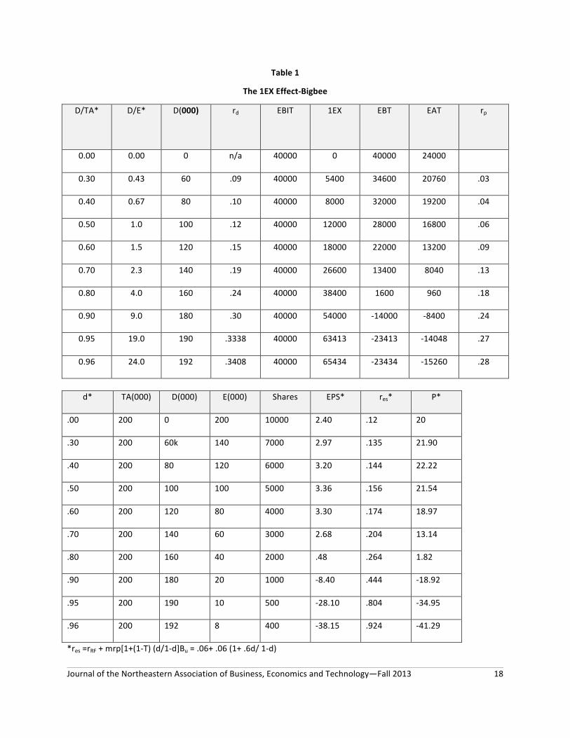
Journal of the Northeastern Association of Business, Economics and Technology—Fall 2013 18
Table 1
The 1EX Effect-‐Bigbee
D/TA*
D/E* D(000)
rd EBIT 1EX EBT EAT rp
0.00 0.00 0 n/a 40000 0 40000 24000
0.30 0.43 60 .09 40000 5400 34600 20760 .03
0.40 0.67 80 .10 40000 8000 32000 19200 .04
0.50 1.0 100 .12 40000 12000 28000 16800 .06
0.60 1.5 120 .15 40000 18000 22000 13200 .09
0.70 2.3 140 .19 40000 26600 13400 8040 .13
0.80 4.0 160 .24 40000 38400 1600 960 .18
0.90 9.0 180 .30 40000 54000 -‐14000 -‐8400 .24
0.95 19.0 190 .3338 40000 63413 -‐23413 -‐14048 .27
0.96 24.0 192 .3408 40000 65434 -‐23434 -‐15260 .28
d* TA(000) D(000) E(000) Shares EPS* res* P*
.00 200 0 200 10000 2.40 .12 20
.30 200 60k 140 7000 2.97 .135 21.90
.40 200 80 120 6000 3.20 .144 22.22
.50 200 100 100 5000 3.36 .156 21.54
.60 200 120 80 4000 3.30 .174 18.97
.70 200 140 60 3000 2.68 .204 13.14
.80 200 160 40 2000 .48 .264 1.82
.90 200 180 20 1000 -‐8.40 .444 -‐18.92
.95 200 190 10 500 -‐28.10 .804 -‐34.95
.96 200 192 8 400 -‐38.15 .924 -‐41.29
*res =rRF + mrp[1+(1-‐T) (d/1-‐d]Bu = .06+ .06 (1+ .6d/ 1-‐d)
Journal of the Northeastern Association of Business, Economics and Technology—Fall 2013 19
Table 2
The 1EX Effect: from Profit to Loss-‐RJR
SALES
EBIT
IEX
EBT
D
E
D/E Pre-‐LBO
Dec. 1986 11517 2009 531 1478 5591 5312 1.05 Dec. 1987 11765 1915 454 1461 4279 6038 0.71 Dec. 1988 12635 2368 549 1818 5518 5694 0.97 LBO 1Q89 2926 402 561 -‐159 29100 2032 14.30 2Q89 3300 547 990 -‐433 26420 1778 14.80 3Q89 2999 452 983 -‐531 25690 1359 18.90 4Q89 3539 652 850 -‐198 25159 1237 20.30 YR89 12764 2053 3384 -‐1330 25159 1237 20.30 1Q90 3204 602 830 -‐228 22937 1024 22.40
Bond
BP
rd%
rRF%
rp% Pre-‐LBO Dec.1986 7 3/8s01 90 1/8 8.57 7.54 1.03 Dec. 1987 8s07 84 7/8 9.73 9.23 0.52 Oct. 1988 8s07 82 4/7 10.06 9.04 1.06 LBO announcement and bidding process Dec. 1988 7 3/8s01 73 ¼ 11.12 8.24 1.88 LBO 1Q89 Anders, p.225 13.71 9.20 4.51 2Q89 Anders, p.225 14.0 8.20 5.80 3Q89 na14.70s07 85 1/4 17.3 8.32 9.07 4Q89 na14.70s08 80 5/8 18.4 8.17 10.25 1Q90 na14.70s08 67 1/8 20.7 8.80 11.98 2Q90 Bond prices vary with rescue rumors. From 10Ks, 10Qs, Annual Reports, Wall Street Journal bond tables. More details in Part 2.
Journal of the Northeastern Association of Business, Economics and Technology—Fall 2013 20
Table 3
Bigbee WACC Results
d
rd
(1-‐T)
Totd
(1-‐d)[rrt+mrp B)
Bu(1+(1-‐T)D/E)
TOTes
WACC
.00 n/a .6 0 1.0[.06+.04(1.500) 1.5(1+.6 x 0)=B .1200 .1200
.30 .09 .6 .0162 .7[.06+.04(1.886) 1.5(1+.6 x 3/7)=B .0948 .1110
.40 .10 .6 .0240 .6[.06+.04(2.10) 1.5(1+.6 x 4/6)=B .0864 .1104
.50 .12 .6 .0360 .5[.06+.04(2.40) 1.5(1+.6 x 1.0)=B .0781 .1140
.60 .15 .6 .0540 .4[.06+.04(2.85) 1.5(1 +.6x1.5)=B .0696 .1236
.70 .19 .6 .0798 .3[.06+.04(3.60) 1.5(1+.6 x 7/3)=B .0612 .1410
.80 .25 .6 .1200 .2[.06+.04(5.10) 1.5(1+.6 x 4)=B .0528 .1728
.90 .30 .6 .1620 .1[.06+.04(9.60) 1.5(1+.6 x 9)=B .0444 .2064
.95
.96
.33
.3408
.6
.6
.1903
.1963
.05[.06+.04(18.60)
.04(.06+.04(23.10))
1.5(1+.6 x 19)=B
1.5(1+.6(24)=B
.0402
.0394
.2305
.2357
Table 4
Summary Table
Simple Regressions t-‐Stat R2 11) Original M&M WACC = 5.3+.006 d 0.75 120 (correlation) 12) Recreated M&M WACC = 5.23+.00655 d 0.77 .120 (correlation) 13) RJR Table 2 WACC = -‐3.68+.1857 d 5.08 .780 14) RJR Table 2 WACC = 4.32+.5371 D/E 13.35 .961 15) RJR + M&M WACC = .58+.0956 d 5.47 .767 16) RJR + M&M WACC = 4.78+.6064 D/E 20.58 .894 Checking for Curvature (M&M Equation 19 format) t-‐Stats R2adj 17) M&M Data WACC = 4.74 + 2.23d -‐ .414d2/1-‐d 1.39 1.15 -‐.016 18) RJR Table WACC = 6.52 -‐ 4.41 + .678d2/1-‐d 2.70 11.11 .978 19) RJR WACC = 6.15 – 13.44d + 22.90d2 1.48 2.85 .798 20) RJR+M&M WACC = 5.92 – 1.60d + .559d2/1-‐d 1.64 16.26 .900
Journal of the Northeastern Association of Business, Economics and Technology—Fall 2013 21
Table 5
WACC Worksheet (D/E and rp from Table 2)
WACC= d (rp+rRFa) (1-‐t) + (1-‐d) (rRFa+mrp B)
D/E 5.080 = .512(1.03+3.71) .60 + .488 (3.71+4*0.929) 1.05 5.126 = .415(0.52+3.71) .60 + .585(3.71+4*0.813) 0.71 5.126 = .492(1.06+3.71) .60 + .508 (3.71+4*0.902) 0.97 10.197 = .935(4.51+3.71) 1 + .065 (3.71+4*8.732) 14.32 11.423 = .937(5.08+3.71) 1 + .063 (3.71+4*9.040) 14.86 14.595 = .950(9.07+3.71) 1 + .05 (3.71+4*11.343) 18.90 15.765 = .953(10.25+3.71)1+.047 (3.71+4*12.164) 20.34 17.469 = .957(11.98+3.71)1+.043(3.71+4*13.338) 22.40 Deduced point: 5.99 = 0 + 1(3.71+4*.57) .00 Notes: rd = rp + rRF (2.35 in 1947-‐48 + 1.36 industry factor to make pre-‐LBO RJR WACC near the M&M 1947-‐48 average). The market risk premium is assumed to be 4% For loss periods T = 0 (Brigham, 2007, p. 339, 332).
Table 6
WACC-‐Capital Structure Regressions
D/D+E SECTION
EQUATION
t-‐statistic
R2adj (*)
.*
21) WACC=5.224+.00661 d (M&M) 0.778 .009 (7) Fig. 7 22) WACC=0.578+.09556 d (combo) 5.471 .367 (8) Fig. 8
23) WACC=3.039+.04834d (M&M+1) 2.685 .126 (9) Fig. 9 D/E SECTION
24) WACC=5.557+0.03066(D/E) .19 -‐.023 (10) Fig. 10 25) WACC=4.778+0.50540(D/E) 20.58 .894 (11) Fig. 11 26) WACC=4.753+0.54003(D/E) 12.77 .791 (12) Fig. 12 *Reference to Figures.
Journal of the Northeastern Association of Business, Economics and Technology—Fall 2013 22
Table 7
The Solution
DATE
SALES
EBIT
IEX
EBT
D
E
D/E
2Q90 3,459 735 797 (62) 22,337 920 24.28 8/17/1990 20,637 2,489 7.88
3Q90 3,529 706 853 (147) 20,075 2,494 8.05 4Q90 3,687 775 746 29 18,675 4,289 4.35 YR90 13,879 2,818 3,226 (408) 18,675 4,289 4.35
4/25/1991 17,049 5,490 3.10 YR91 14,989 2,934 2,217 717 14,337 8,419 1.70 YR92 15,734 2,906 1,449 1,457 14,124 8,376 1.69
DATE Bond BP rd% rRF% rp% D/E 7/16/1990 17s07 1000reset 17.00 8.80 8.20 7.88 4/25/1991 1.050s?? 1,000 10.50 8.29 2.21 3.10 Apr-‐92 8.50s?? 1,000 8.50 6.90 1.60 1.70 Jan-‐93 8s?? 1,000 8.00 6.63 1.37 1.69
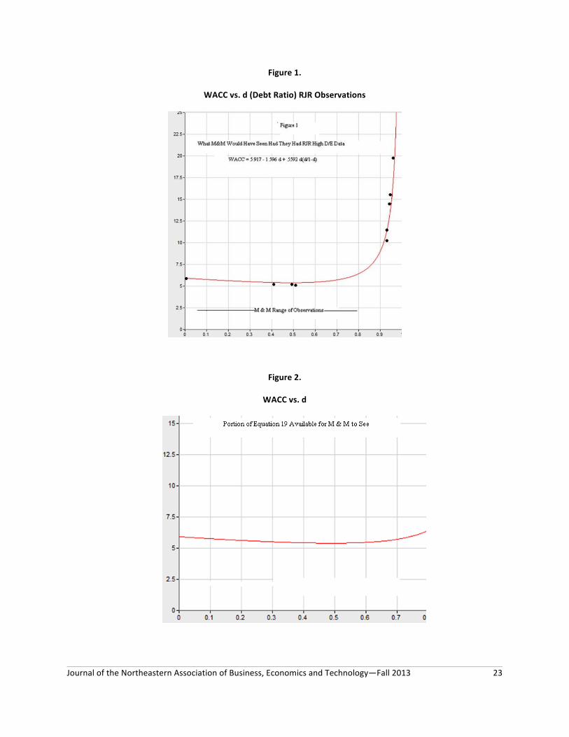
Journal of the Northeastern Association of Business, Economics and Technology—Fall 2013 23
Figure 1.
WACC vs. d (Debt Ratio) RJR Observations
Figure 2.
WACC vs. d
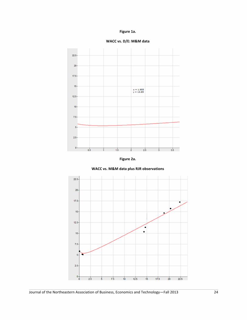
Journal of the Northeastern Association of Business, Economics and Technology—Fall 2013 24
Figure 1a.
WACC vs. D/E: M&M data
Figure 2a.
WACC vs. M&M data plus RJR observations
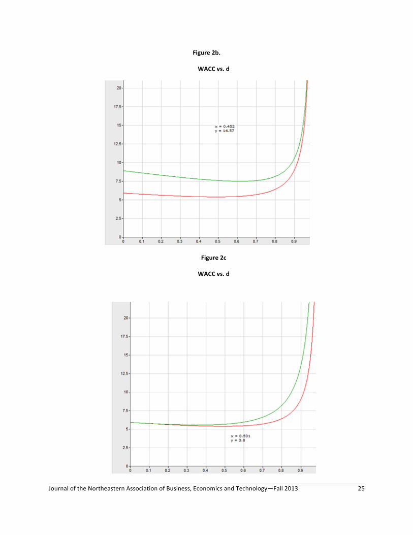
Journal of the Northeastern Association of Business, Economics and Technology—Fall 2013 25
Figure 2b.
WACC vs. d
Figure 2c
WACC vs. d

Journal of the Northeastern Association of Business, Economics and Technology—Fall 2013 26
Figure 3
Risk Premium vs. D/E
Figure 4
Risk Premium vs. log D/E
There is a problem with Fisher’s equation (Analytical Tools section). The coefficient of variation of earnings
was done on earnings after tax basis. It would have been preferable to use EBIT because
Figure 5
WACC vs d=d/D/E
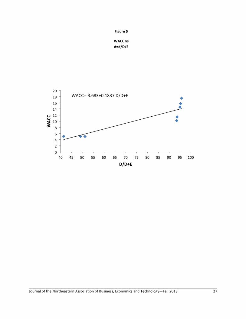
Journal of the Northeastern Association of Business, Economics and Technology—Fall 2013 27
Figure 5
WACC vs d=d/D/E
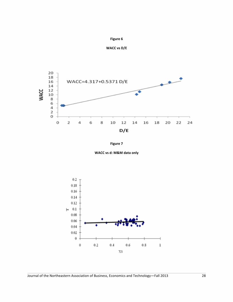
Journal of the Northeastern Association of Business, Economics and Technology—Fall 2013 28
Figure 6
WACC vs D/E
Figure 7
WACC vs d: M&M data only
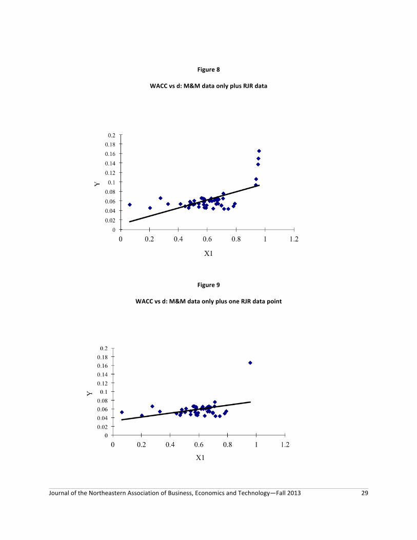
Journal of the Northeastern Association of Business, Economics and Technology—Fall 2013 29
Figure 8
WACC vs d: M&M data only plus RJR data
Figure 9
WACC vs d: M&M data only plus one RJR data point
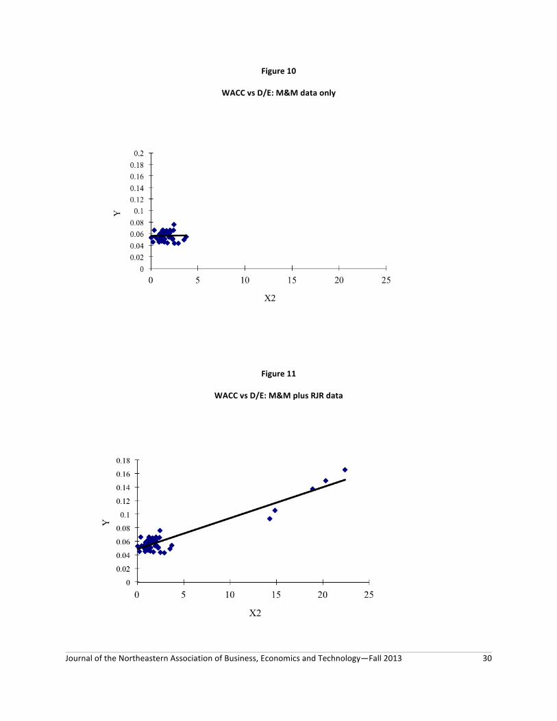
Journal of the Northeastern Association of Business, Economics and Technology—Fall 2013 30
Figure 10
WACC vs D/E: M&M data only
Figure 11
WACC vs D/E: M&M plus RJR data
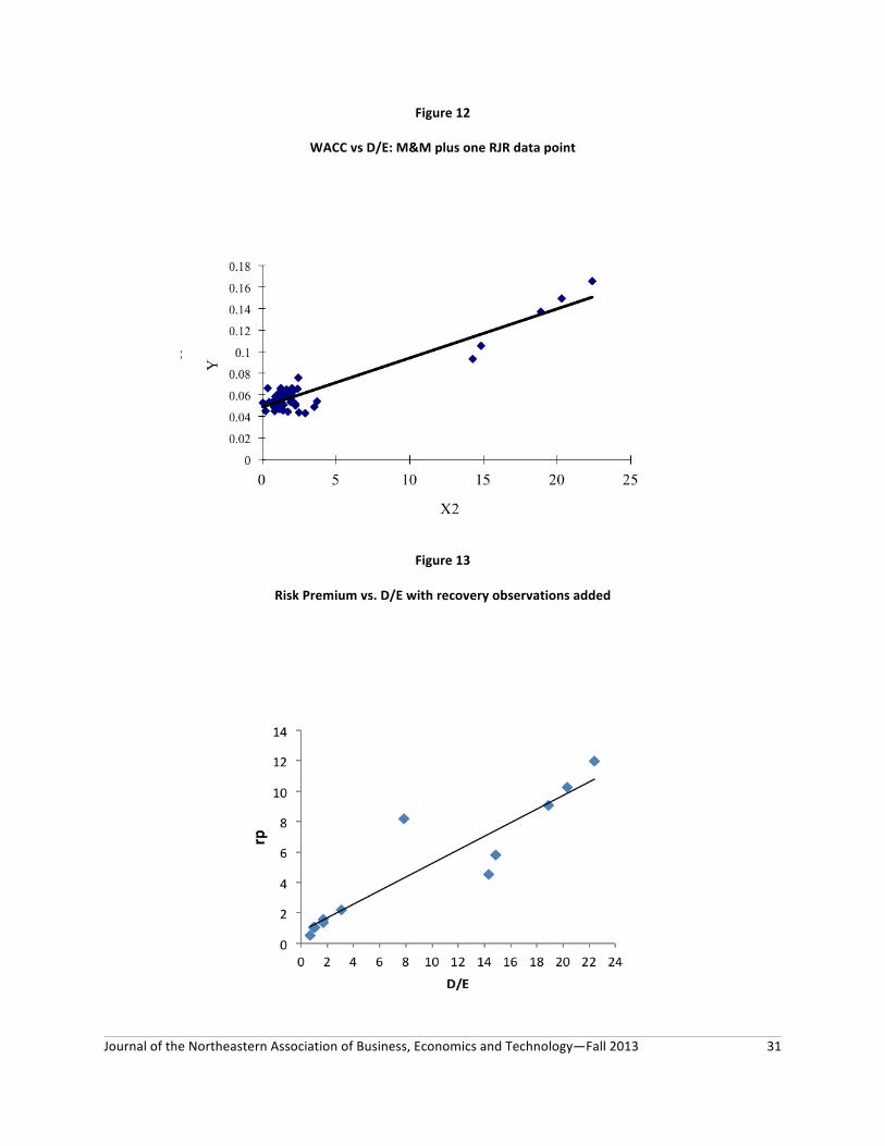
Journal of the Northeastern Association of Business, Economics and Technology—Fall 2013 31
Figure 12
WACC vs D/E: M&M plus one RJR data point
Figure 13
Risk Premium vs. D/E with recovery observations added

Journal of the Northeastern Association of Business, Economics and Technology—Fall 2013 32
William Carlson, PhD has been a finance professor at Duquesne University for 41 years. His interests are investment analysis and macro financial policy.
Conway Lackman, PhD has been a marketing professor at Duquesne University for 20 years. His interests are marketing models and their impact on financial performance.
The authors are indebted to Chrissy Chapman, Chris Koenig, Xiaomei Min, and Steve Sinnott for their data and graphic support.
Journal of the Northeastern Association of Business, Economics and Technology—Fall 2013 33
RATIO ANALYSIS AT PRIVATE COLLEGES AND UNIVERSITITES IN PENNSYLVANIA
Michael J. Gallagher
ABSTRACT This paper provides a comparison of financial ratios for the year ended June 30, 1997 to financial ratios for the year ended June 30, 2011 at 10 non-selective private liberal arts based colleges and universities. Gallagher (1999) provided a summary of ratios at 34 private non-selective liberal arts colleges in Pennsylvania and Ohio for the fiscal years ended June 30, 1997 and June 30, 1996. The original paper was designed to discuss the changes to financial reporting because of the incorporation of Financial Accounting Standards Boards (FASB) Statements 116, 117, and 124. This paper provides business officers at private colleges and universities benchmark comparisons of the changes in areas of financial measurement contained in the annual reports of these institutions including affordability, changes in expenditures, financing issues, revenue sources, and the ratios used by the United States Department of Education to measure the viability of the institutions.
INTRODUCTION
The financial plight of private higher education
has long been a concern of trustees, as well as enlightened governors, higher education coordinating agencies, and legislators. Rudolph (1990) described private non-selective liberal arts colleges that were kept afloat financially by paying their professors with produce begged from neighboring farmers. Toward the end of the “baby boom” of the 1960s experts expressed concern of an impending demise of the independent sector, due in part to declining high school graduating classes and the establishment of cheaper public college and university alternatives. Clearly, upon entering the 1990s, the fiscal health of independent institutions of higher education continued to be of concern to federal and state policy-makers. In 1991, the Education Commission of the States weighed in with its report, The Essential Role of Private Colleges and Universities, co-chaired by John Ashcroft and Clark Kerr, former Chairman of the Carnegie Commission on Higher Education. This report strongly endorsed expanded state student financial aid programs, deeming the state’s role in preserving private higher education to be important. The launching of the American Council on Education’s “College is Possible” program, designed to allay concerns over the misinformation that parents and students receive regarding availability of financial aid for college, was directly due to heightened concerns over college affordability (American Council on Education 1999).
Comparing the fiscal health of independent institutions of higher education has always been a concern of the trustees at their institutions. It has also become an on-going concern of forward-thinking state and federal policy-makers, and indeed, anyone who recognizes the vital role played by this nation’s vibrant private sector of higher education. The purpose of this article is to analyze the financial performance of ten private colleges and universities in Pennsylvania and Ohio for the years ended June 30, 2011. This analysis will be compared to a 1999 (Gallagher) dissertation that analyzed the same colleges. The financial ratios for 1997 will be compared to the 2011 ratios to analyze the changes in the financial position and results of operations for these universities. The discussion of key implications and benchmark results will be useful for business officers in determining their comparable success in the previous 14 years. Financial statements are important to trustees and institutions for a variety of reasons. First, in order to qualify as an institution that can administer federal student financial aid in this country, institutions submit information from their financial statements to the U.S. Department of Education and the Internal Revenue Service. Because student financial aid from all sources approached $60 billion in 1997-98, providing millions of students with both access and choice to the world’s most diverse set of higher education institutions, virtually all independent institutions submit their financial statements (American Council on Education, 1999). Second, to qualify for state supported student financial aid as well as to meet legal corporate registration
Journal of the Northeastern Association of Business, Economics and Technology—Fall 2013 34
requirements, most independent institutions submit their financial statements to the corresponding state’s higher education coordinating agency in the state in which the institution is chartered. Third, donors are interested in the financial statements of institutions to see if the institution manages its resources well, and is worthy of receiving substantial endowment investments. Fourth, trustees care about being able to “benchmark” the relative performance of their institutions to one another. Finally, since trustees are individually and collectively liable for inaccurate financial reporting, they have a legal obligation to foster accurate financial reporting that goes beyond their responsibility to provide good, sound management.
This paper will provide a framework of a methodology to interpret the results of operations and the financial position of these institutions. The ratios in Tables 1 – 8 measure affordability, changes in expenditures, changes in financing, revenue sources, and the financial viability of 10 private colleges and universities. Affordability of Baccalaureate Arts II Colleges and Universities
The tuition costs at colleges and universities have been discussed because of the recent economic downturn and the budget deficits of the states. The general tone is that college costs are growing at a rate higher than inflation. President Obama stated on January 27, 2012 to an audience at the University of Michigan at Ann Arbor that “If you can’t stop tuition from going up, then the funding that you get from taxpayers will be going down” (Obama, B., 1/27/2012). This statement by President Obama may be true of public universities and private highly selective liberal arts colleges. The colleges and universities in this study contradict President Obama statement as it applies to non-selective liberal arts colleges and universities.
The results of Table 1 illustrate that the ten “tuition driven” colleges calculate an increase in net tuition at a rate below the consumer price index from 1997 to 2011. Table 1 indicates that tuition increased 2.60 times but the financial aid increased 3.27 times causing an increase in the net tuition to be 2.37 times. The consumer price index (CPI) during this same period of time (1997 -2010) increased 2.39 times (Annualized Growth Rates and Graphs, 2011). Public policy and public opinion should take note that the colleges, with a smaller amount of endowment support (as compared to the elite colleges) and with less support from the public (as compared to the public universities), have been able to control their increase in net tuition support from the students. This may be a result of increased market pressures caused
by the changing landscape of higher education rather than a concerted effort to limit the increase in net revenue.
The result of the recent economic crises has caused private colleges to limit increases in tuition pricing. “At the beginning of the economic downturn, many institutions increased tuition minimally or not at all, hoping to maintain their enrollments. The enrollments did remain stable, a result of both pricing and increases in acceptance rates to ensure that more students would enroll” (Nelson, L., 2010). These colleges and universities are also controlling costs at their institutions but the methods of controlling cost may be at the expense of the competitive advantage of the small liberal arts college.
Expenditure increases at private colleges and universities
The tuition discount increase to 37% from 31% indicates that these colleges and universities are spending more on institutional financial aid and less on instructional and student programming. One of the ways that colleges and universities accomplish this reallocation of funding is by using additional part time instructors and less tenure track full time college professors. According to McArdle (2012) adjunct professors are helpful budget-wise as, “It’s a pool of cheap labor for the university”. The current economics of the non-selective liberal arts colleges require additional institutional financial aid to attract the freshman class along with retaining the returning students at their colleges and universities. They are finding ways to cut the budget in areas critical to the mission of the college.
The expenditures have increased 2.12 times over the 14 year period (Table 2). The increase of 12.7% ((2.39 – 2.12)/2.12) is less than the increase in the CPI from 1997 to 2010 of 2.39 times. “Colleges and universities in resource-poor institutions are likely to feel increasingly overwhelmed and demoralized by the growing institutional demand placed on them and their inability to identify sufficient resources to maintain traditional levels of support for undergraduate education” (Arum, R. and Roksa, J, 2011). The data indicates that non-selective liberal arts colleges and universities are spending more of their resources in attracting students to their campuses by discounting tuition and cutting the expenses of their operations. Table 2 indicates that the unrestricted net assets of these colleges and universities have not increased at the same rate as the increase in expenses. The average ratio of unrestricted net assets to expenses in 2011 has decreased from .92 in 1997 to .88 in 2011. The increase in expenditures was 2.12 but the
Journal of the Northeastern Association of Business, Economics and Technology—Fall 2013 35
increase in the unrestricted net assets was 1.97. This indicates that the colleges are spending less money on their mission and are losing the financial flexibility to change operations to more profitable areas because of the proportional decrease in the unrestricted net assets. Unrestricted net assets at a private institution act like the retained earnings of the corporation. The retained earnings of the corporation provide a buffer for entities to accumulate funds for purchasing property, plant and equipment or to take advantage of an opportunity with a high rate of return.
Table 3 indicates that these institutions may be funding the infrastructure at a higher level because the temporarily and permanently restricted net assets are growing at a rate higher than the inflation rate. The increase of 3.27 times of the temporarily and permanently restricted net assets is 1.3 times higher than the 1.97 times increase in unrestricted net assets. This may be caused by colleges and universities adding to the infrastructure rather than carrying the cost savings of reducing expenditures to the unrestricted funds. Institutions may be spending less on salaries and other operating costs but may be adding buildings and facilities to remain competitive. Standard and Poor’s reported in 2006 a university construction boom and described this increase as an arms race. The implication is that the spending was tangential to their educational mission and expensive to build and maintain (The Economist, 2012).
The “arms race” metaphor may apply to the selective colleges and universities but it may be survival for the colleges in this study. These colleges must compete with both institutional financial assistance and by providing the facilities that will attract students to their institutions. The result is better facilities but at the expense of keeping the current facilities viable and the ranks of the professoriate strong.
Financing of colleges and universities The colleges and universities in this study illustrate the increased construction on the campuses of the private institutions especially student housing options and fitness facilities. Each college needs to add or update their living and recreational facilities to keep up with the other colleges who are also adding to the infrastructure. These colleges are building to stay competitive when a high school senior tours the campus. The fitness facilities and new living space for the next generation of students is increasingly being built with new debt. Table 4 and 5 illustrate that the unrestricted net assets and the total net assets of these universities are decreasing as compared to the debt of the colleges. The unrestricted net assets decreased from 1.62 times to 1.50 times the amount
of debt and the total net assets decreased from 2.81 to 2.60 times the amount of debt. The long-term debt increased 2.48 times from 1997 to 2011. This increase is higher than the consumer price index (CPI) increase of 2.37 times (Annualized growth rates and graphs, 2011). The increase in unrestricted net assets (1.97) and total net assets (2.32) illustrate an increase in the net asset base at a rate that is lower than the CPI and more importantly at a rate significantly lower than the increase in the debt of the colleges and universities. The net assets of the not-for-profit are similar to the owners’ equity of the for-profit corporation because it is the portion of the assets of the entity that is not claimed by the creditors. This would mean that these institutions have increased risk caused by a higher asset base. The increased building on campuses may come at the expense of the operating budgets of the institution but the buildings are built to attract donations and students. This increase in building is attracting the attention of the bond rating agencies and the federal government. Johnson (2012) noted, “They get very concerned when they see a college our size doing this much building at one time.” The private college and university sector may experience their own housing bubble as they continue to build facilities (many funded by donors) on their campuses with the hope of adding to their revenue base by attracting more students and donors. The donors want their name on facilities but the deferred maintenance grows because the institutions do not have the operating budget to run their existing facilities and the new facilities will add to this burden. The increase in building is increasingly going towards student housing and fitness facilities. The “arms race” is evident in the building of fitness facilities or adding to the existing facilities. Colleges and universities are building architecturally beautiful facilities with climbing walls, fitness rooms for aerobics along with self-defense classes. These institutions must have these facilities because their competition has built or is in the process of building a new fitness building. These fitness rooms have TVs on the treadmills, juice bars for socializing after your workout or instead of the workout (Recreation Management, 3/6/2012). Another reason for the increase in the fitness facilities is that many of the colleges in this study rely on sports programs to recruit their freshman class. These sports teams need a place to prepare for their sports seasons. The spring season requires indoor facilities because the start of the season is February and March. A time of the year that may make outside practices impractical. The building of student living facilities contributes to the debt load and the building on college campuses. Colleges competing for students
Journal of the Northeastern Association of Business, Economics and Technology—Fall 2013 36
are constructing better student housing to attract the freshman class. Colleges and universities are designing the new residence halls to attract students and provide the students with living arrangements designed for comfort rather than areas that help shape their social and academic development at college. The university looks at the room and board charges as revenue centers and may even outsource the operations to private for-profit companies. The new living area may be a private-suite arrangement that will cater to students demand for privacy and comfort and the institutions goal of creating a profit center (Arum, R. and Roksa, J. 2011). The elite colleges and universities are able to provide these luxuries to attract students with the academic profile that will advance their status in the college rankings. Struggling tuition driven colleges may need to cut costs in other areas to pay for this arms race and the increased financial aid necessary to compete for students to enroll in their freshman class. Sources of Revenues
Colleges and universities have several sources of income including tuition, room charges, board charges, endowment income, government grants, and other miscellaneous income streams. The colleges analyzed derive the majority of their income from tuition revenue. This type of college is designated as a “tuition driven” school. The elite colleges derive revenue for their operations from tuition but the tuition revenue does not cover the cost of educating the students. Endowment income supplements the tuition revenue at these elite private colleges. These colleges will have a waiting list of students to accept a spot in the institution if other students decline their admissions offer. The public universities are supported by state governments. The non-selective liberal arts colleges are (in most cases) not operating at full capacity and do not have the diversity of funding options that exists at the elite colleges and the public universities.
Table 6 demonstrates the decrease in the change in net assets from educational sources as compared to the total revenues from these sources. The pressure of “making the freshman class” is causing these colleges to show a decreasing margin in their major revenue sustaining activity. The 42% decrease in margin (.19 to .11) illustrates a potential problem for these colleges and universities. They may be experiencing pressure from the more selective colleges offering admissions to their potential top students. “The median selectivity rate rose to nearly 61% from 57%” (Stripling, J. 4/11/2012). The trend is that the selective colleges are admitting students who may have attended the non-selective universities. The non-selective colleges may also be
experiencing pressures from the for-profit colleges that are able to operate with lower per student expenses. In addition, students now are taking college level courses in high school and on-line courses during summers and even during the semesters. This is causing a significant decrease in the margin for the principle revenue source of the institutions in this study (Table 6).
The colleges and universities in this study have compensated for the decreasing margins in tuition and revenue sources by increasing their margins in the auxiliary enterprises of the institution. This is helping to keep the colleges afloat much like the early days of the United States history in higher education. Table 7 calculates a 33% increase in the margins for the auxiliary enterprises of the non-selective liberal arts colleges. One of the potential problems with this mix of profit margins is that it may cause these colleges to focus on other issues rather than their educational mission of providing undergraduate education to the traditional college age student. When the profit margins of ancillary products increase the entity may focus more on these activities at the expense of the primary mission. Colleges and universities will rent their new fitness facilities and the student living facilities for conferences and sports tournaments resulting in students at the institutions possibly not being able to use the facilities that attracted them to the college.
Colleges and universities are also outsourcing many of the support processes at the institutions of higher education. This may be a short term method of keeping the college viable but potential long term changes may alter the strategic plan of the university. Bookstore, food service, security, dormitories, information technology, and other support products have been outsourced to for-profit companies. These for-profits are looking at the “bottom line” causing the services to be offered as value added only if they increase profit. These support activities when operated by the college would have a strategy of supplementing the educational mission. This may decrease the appeal of attending the small liberal arts college in the future because of increased expenses at the bookstore and cafeteria, and without the potential learning opportunities these functions may provide. Department of Education Ratios
The United States Department of Education (DOE) received a report from the accounting firm KPMG Peat Marwick LLP on August 1, 1996 “to assist the DOE in developing an improved methodology, using financial ratios, that could be used both as an initial screening device to identify financially troubled institutions and as a mechanism for efficiently exercising its financial oversight
Journal of the Northeastern Association of Business, Economics and Technology—Fall 2013 37
responsibility” (KPMG Peat Marwick LLP, August 1, 1996). This report started my analysis of non-selective private colleges and universities resulting in the book “Using financial statement analysis to assess economic conditions at non-selective liberal arts colleges” (Gallagher, 1999). These ratios are now being used by the United States Department of Education (DOE) to measure the viability of private colleges and universities. Table 4 provides an analysis of the financial viability of the colleges and universities in this study while Table 8 provides an analysis of the primary reserve ratio of these institutions. The ratios in these two tables provide 90% of the data for identifying a financially troubled institution. The other 10% was a net income ratio. This paper excludes this ratio because of the not-for-profit nature of the institutions. This ratio was added by the Department of Education (DOE) because the DOE also analyzes the for-profit higher education sector.
The viability ratio decreased 7% from 1997 to 2011 (1.50 in 2011 compared to 1.62 in 1997 see Table 4) and the primary reserve ratio decreased 37% from 1997 to 2011 (.83 to .52 see Table 8). The viability and primary reserve ratios are ratios that measure the ability of the entity to be successful in the long term. “A total of 149 nonprofit colleges failed the department of education’s test of financial strength in 2009” (Blumenstyk, G. & Richards, A., 2010). “This means that these colleges must post letters of credit equal to at least 50 percent of the funds they receive from financial aid” (Blumenstyk, G. & Richards, A. 2010). One of the colleges is this analysis was on this list for additional requirements because the DOE considers this college to be “financial troubled”.
The cause of many of the colleges and universities on this list may be timing issues. This dilemma relates to the construction projects on the campus because funding a campus construction project causes the institution to increase its asset base. “When liquid assets such as cash or investments are converted to fixed assets, the primary reserve ratio may be negatively affected in the year of conversion” (BKD CPAs &Advisors, 10/2010). Endowment returns may also affect these ratios although many of the colleges and universities that struggle with the ratios do not have a large endowment but base their success on tuition and fees from the students.
One of the other potential issues that the private college and university sector may experience is the possibility of takeovers from for-profit organizations. “A failing score has also become a signal to investors that an institution could be ripe for takeover by a for-profit company” (deVise, D., 5/21/2012). Private colleges and universities are experiencing many
challenges in the competitive industry sector of higher education including an increased focus by the Department of Education relating to the ability of an institution to remain viable in the future.
CONCLUSION
The future plight of “tuition driven” colleges and
universities seems to be dire. Previously, these institutions have been able to survive for several centuries and provide a valuable education for many students. Several of these early colleges developed into the top universities in the world including Harvard, Stanford, Columbia, Yale and the University of Pennsylvania. These universities have the top five growth rates in endowment from 2002-2008 according to the Chronicle of Higher Education. The problem according to this same article is that while Yale has increased its endowment by 119% during this time frame the bottom quarter has had a decrease of 13% and the third quarter a decrease of 4.1% while the first quarter increased 7% (the universities with the highest endowment) and the second quarter 4%. “The one-year change in amount raised was progressively worse among colleges that raised less money” (The Chronicle of Higher Education, March 6, 2009).
The colleges in this survey will also be affected by state appropriation changes. According to the Chronicle of Higher Education, “states are tightening financing despite a boost from stimulus money” (The Chronicle of Higher Education, 1/18/2010). The average of all the states is a decrease of 1.1% while Ohio has a 7.9% decrease and Pennsylvania has a 3.8% decrease (The Chronicle of Higher Education, 2010). This illustrates that the universities in this survey are receiving less money in their fundraising efforts and less money from state appropriations.
The third pressure on these colleges and universities is the “vulnerability to lower-cost alternatives among public colleges and community colleges” (The Chronicle of Higher Education, January 16, 2009). For-profit and on-line delivery of courses may also add to the dilemma of the institutions in this survey. According to the Chronicle of Higher Education, “Moody’s is particularly concerned about small, tuition-dependent private colleges and some regional public universities facing serious challenges to their continued financial viability”.
Private “tuition driven” colleges and universities in Ohio and Pennsylvania are going to survive by being efficient and focusing on a particular niche. “The colleges that will emerge as winners will have strong leadership” (Fain, 2010). Colleges without this strong leadership may not survive the current economic environment. Moody’s states that a
Journal of the Northeastern Association of Business, Economics and Technology—Fall 2013 38
“college with a president that dominates the conversation and is pretty much a salesman, spinning mode the whole time would almost be certainly downgraded” (Fain, P. 11/22/2010). The colleges that will thrive will create a strategic plan with efficient use of resources and a focus on “value added” activities that will differentiate their university and provide a unique product to the diverse higher education industry.
The “value added” premise of the increase in higher education may be changing based on the recent pressures on the industry. The increase of the percentage of Americans with a college degree from 5% in 1944 to 40% today has possibly backfired (Samuelson, May 27, 2012). This increase in college attendance may have caused society to value the degree not the skills and knowledge behind the degree (Samuelson, May 27, 2012). The colleges and universities that will be successful in the future are the institutions that are able to compete on the academic quality of their university. Competition has increased in the higher education industry and the colleges and university that are creating their own niche will be successful.
REFERENCES
American Council on Education (1999, March 8).
Available at: http://www.collegeispossible.org/ Annualized Growth Rates and Graphs Homepage of
Measuring Worth (12/19/2011). [Online]. Available: http://www.measuringworth.com/growth/growth_resultf.php?US%5B%5D=DOLLAR&begin%5B%5D=1997&end%5B%5D=2010&beginP%5B%5D=&endP%5B%5D
Arum, R. and Roksa, J. (2011). Academically Adrift:
Limited Learning on College Campuses (p. 128). Chicago, IL: The University of Chicago Press
Ashcroft, J., & Kerr, Clark (1990). The preservation
of excellence in American higher education: the essential role of private colleges and universities. Denver CO: Education Commission of the States.
BKD CPAs & Advisors, (10/2010). Industry
Insights: Private colleges struggle with Department of Education Ratios. [Online] Available:
http://www.bkd.com/articles/2010/private-colleges-struggle-with-department-of-education-ratios.htm
Blumenstyk, G. & Richards, A (8/11/2011). 149 Nonprofit colleges fail education department’s test of financial strength. [Online] Available http://chronicle.com/article/150-Nonprofit-Colleges-Fail/123878/
The Chronicle of Higher Education (1/18/2010).
State Financing Tightens Despite Boost from Stimulus. [Online] Available: http://chronicle.com/article/Interactive-Map-State/63644/
The Chronicle of Higher Education (3/6/2009).
Giving to Colleges and Universities, 2007-2008: Winners and Losers in Funds Raised. [Online] Available: http://chronicle.com/article/fund-raising-by-colleges-and/30610
The Chronicle of Higher Education (1/16/2009).
Moody’s Forecasts Stiff Challenges, Especially for Private Colleges, in the Next Year. [Online] Available: http://chronicle.com/article/Moodys-Forecasts-Stiff-Cha/32953?
deVise, D (5/21/2012). College Inc.: 150 private
colleges fail DOE financial test. [Online] Available: http://voices.washingtonpost.com/college-inc/2010/08/150_private_colleges_fail_ed_f.html
The Economist (3/1/2012). Construction on Campus; Just Add Cash, The great expanding American University. [Online] Available: http://www.economist.com/node/10216515?story_id=10216515&CFID=2483925&CFTOKEN=92d6020a4065b8ae-A129FBB5-B27C-BB00-01277E3E517138B9
Fain, P. (11/22/2010). The Chronicle of Higher
Education Leadership and Governance: Moody’s Report Shines Spotlight on College Leaders Amid Bleak Financial Outlook [Online] Available: http://chronicle.com/article/article-content/125469
Gallagher, M. J. (1999). Using financial statement
analysis to assess economic conditions at non-selective liberal arts colleges, Proquest UMI Dissertations International.
Johnson, M. (3/6/2012). Private Colleges Build
Facilities to Attract Donations and Students. Finance and Commerce [Online] Available: http://finance-commerce.com/2011/09/private-colleges-build-facilities-to-attract-donations-and-students/

Journal of the Northeastern Association of Business, Economics and Technology—Fall 2013 39
KPMG Peat Marwick LLP (8/1/1996). Financial Ratio Analysis Project Final Report. [Online] Available: http://www2.ed.gov/finaid/prof/resources/finresp/ratio/full.pdf
McArdle, E. (3/1/2012). The Adjunct Explosion.
University Business [Online] Available: http://universitybusiness.ccsct.com/page.cfm?p=159
Nelson, L. (1/19/2010). Financial Outlook Remains
Negative for Higher Education, Moody’s Says. [Online] http://chronicle.com/article/Financial-Outlook-Remains/63642/
Obama, B. (1/27/2012). Remarks by the President on
College Affordability, Ann Arbor, Michigan. [Online] http://www.whitehouse.gov/the-press-office/2012/01/27/remarks-president-college-affordability-ann-arbor-michigan
Recreation Management (3/6/2012). A Look at trends in Recreation at Colleges and Universitites. [Online] Available: http://recmgmt.com/feature_print.php?fid=201106fe05
Rudolph, F. 1990. The American college and
university. Athens, GA: The University of Georgia Press: 194.
Samuelson, R.J. (5/27/2012). Ditch College for all. [Online] Available: http://mobile.washingtonpost.com/rss.jsp?rssid=4223411&item=http%3a%2f%2fwww.washingtonpost.com%2fopinions%2fits-time-to-drop-the-college-for-all-crusade%2f2012%2f05%2f27%2fgJQAzcUGvU_mobile.mobile&cid=-1
Stripling, J. (4/11/2012). Revenue Dip for Private
Colleges. [Online] Available: http://www.insidehighered.com/print/news/2009/11/03moodys
Journal of the Northeastern Association of Business, Economics and Technology—Fall 2013 40
Table 1
Tuition Discount Analysis
Tuition Increase
Financial aid increase
Net tuition increase
Tuition Discount Ratio 2011
Tuition Discount Ratio 1997
College 1 2.72 3.42 2.31 .46 .37
College 2 2.04 2.75 1.66 .47 .35
College 3 2.43 2.68 2.31 .36 .33
College 4 2.72 3.34 2.46 .36 .30
College 5 2.66 2.79 2.59 .40 .38
College 6 2.33 2.96 2.10 .35 .28
College 7 1.91 1.97 1.88 .32 .31
College 8 4.64 7.52 4.14 .24 .15
College 9 2.48 2.53 2.45 .40 .39
College 10 2.09 2.72 1.86 .36 .27
Average 2.60 3.27 2.37 .37 .31
Table 2
Comparison of unrestricted net assets to expenses
Increase in expenses
Increase in unrestricted net assets
Unrestricted net assets to expenses 2011
Unrestricted net assets to expenses 1997
College 1 2.09 3.48 1.29 .78
College 2 2.02 1.10 .93 1.71
College 3 2.21 3.04 .85 .62
College 4 1.85 1.59 2.22 2.58
College 5 2.03 1.54 .73 .96
College 6 1.74 1.62 .49 .43
College 7 1.60 1.80 .34 .30
College 8 3.85 3.25 .80 .17
College 9 2.08 1.55 1.01 1.02
College 10 1.77 .73 .13 .61
Average 2.12 1.97 .88 .92
Journal of the Northeastern Association of Business, Economics and Technology—Fall 2013 41
Table 3
Comparison of temporarily and permanently restricted net assets to expenses
Increase in expenses
Increase in temporarily and permanently restricted net assets
Temporarily and permanently restricted net assets to expenses 2011
Temporarily and permanently restricted net assets to expenses 1997
College 1 2.09 3.42 1.03 .85
College 2 2.02 2.75 1.83 1.03
College 3 2.21 2.68 .52 .36
College 4 1.85 3.34 .57 .40
College 5 2.03 2.79 .88 .69
College 6 1.74 2.96 1.10 1.03
College 7 1.60 1.97 .80 .51
College 8 3.85 7.52 .22 .17
College 9 2.08 2.53 1.17 1.02
College 10 1.77 2.72 1.08 .61
Average 2.12 3.27 .92 .67
Table 4
Comparison of unrestricted net assets to long term debt
Increase in long term debt
Increase in unrestricted net assets
Unrestricted net assets to long term debt 2011
Unrestricted net assets to long term debt 1997
College 1 2.87 3.48 1.91 1.58
College 2 4.01 1.10 .75 2.73
College 3 1.81 3.04 1.93 1.15
College 4 .90 1.59 3.38 1.92
College 5 2.40 1.54 .80 1.25
College 6 1.79 1.62 .89 .98
College 7 1.82 1.80 .45 .45
College 8 4.55 3.25 .79 1.10
College 9 2.73 1.55 1.79 3.16
College 10 1.87 .73 2.32 1.86
Average 2.48 1.97 1.50 1.62
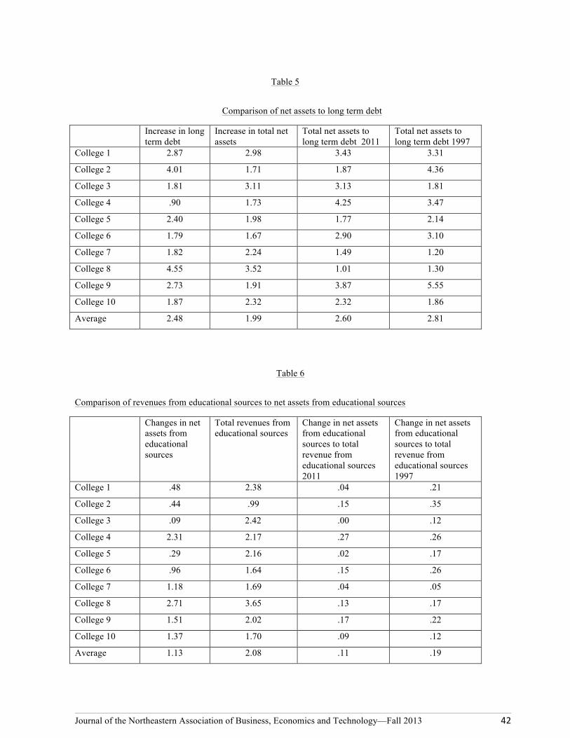
Journal of the Northeastern Association of Business, Economics and Technology—Fall 2013 42
Table 5
Comparison of net assets to long term debt
Increase in long term debt
Increase in total net assets
Total net assets to long term debt 2011
Total net assets to long term debt 1997
College 1 2.87 2.98 3.43 3.31
College 2 4.01 1.71 1.87 4.36
College 3 1.81 3.11 3.13 1.81
College 4 .90 1.73 4.25 3.47
College 5 2.40 1.98 1.77 2.14
College 6 1.79 1.67 2.90 3.10
College 7 1.82 2.24 1.49 1.20
College 8 4.55 3.52 1.01 1.30
College 9 2.73 1.91 3.87 5.55
College 10 1.87 2.32 2.32 1.86
Average 2.48 1.99 2.60 2.81
Table 6
Comparison of revenues from educational sources to net assets from educational sources
Changes in net assets from educational sources
Total revenues from educational sources
Change in net assets from educational sources to total revenue from educational sources 2011
Change in net assets from educational sources to total revenue from educational sources 1997
College 1 .48 2.38 .04 .21
College 2 .44 .99 .15 .35
College 3 .09 2.42 .00 .12
College 4 2.31 2.17 .27 .26
College 5 .29 2.16 .02 .17
College 6 .96 1.64 .15 .26
College 7 1.18 1.69 .04 .05
College 8 2.71 3.65 .13 .17
College 9 1.51 2.02 .17 .22
College 10 1.37 1.70 .09 .12
Average 1.13 2.08 .11 .19
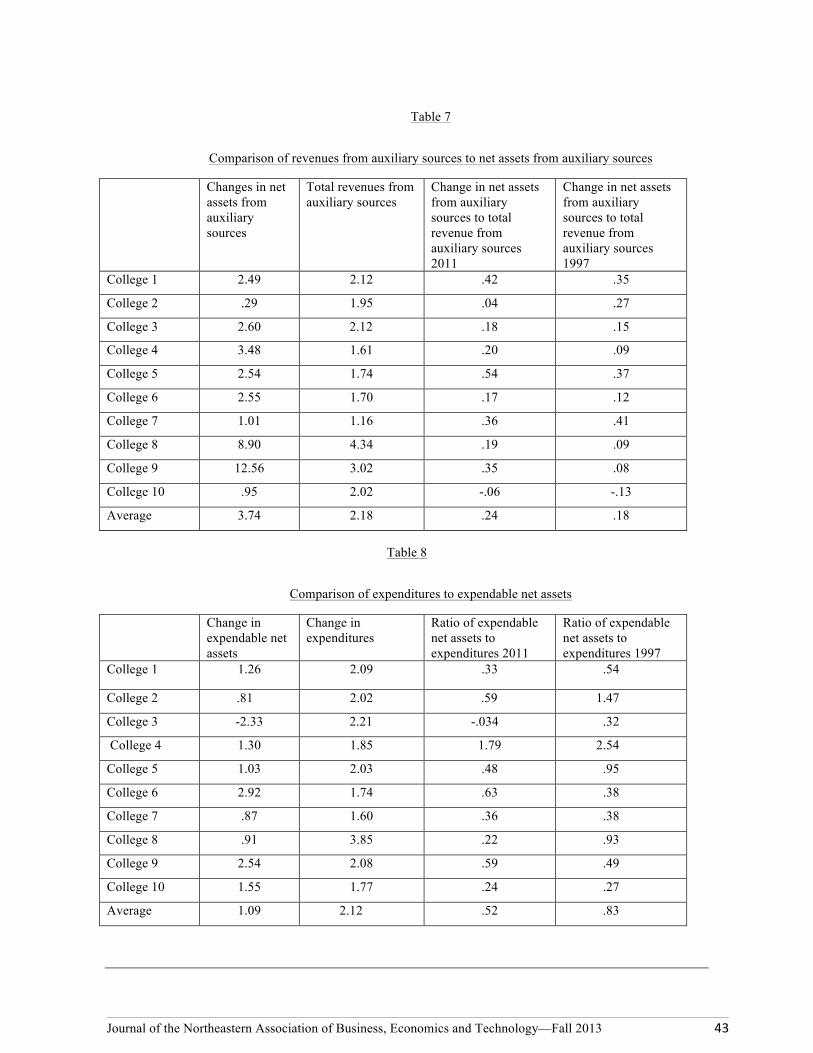
Journal of the Northeastern Association of Business, Economics and Technology—Fall 2013 43
Table 7
Comparison of revenues from auxiliary sources to net assets from auxiliary sources
Changes in net assets from auxiliary sources
Total revenues from auxiliary sources
Change in net assets from auxiliary sources to total revenue from auxiliary sources 2011
Change in net assets from auxiliary sources to total revenue from auxiliary sources 1997
College 1 2.49 2.12 .42 .35
College 2 .29 1.95 .04 .27
College 3 2.60 2.12 .18 .15
College 4 3.48 1.61 .20 .09
College 5 2.54 1.74 .54 .37
College 6 2.55 1.70 .17 .12
College 7 1.01 1.16 .36 .41
College 8 8.90 4.34 .19 .09
College 9 12.56 3.02 .35 .08
College 10 .95 2.02 -.06 -.13
Average 3.74 2.18 .24 .18
Table 8
Comparison of expenditures to expendable net assets
Change in expendable net assets
Change in expenditures
Ratio of expendable net assets to expenditures 2011
Ratio of expendable net assets to expenditures 1997
College 1 1.26 2.09 .33 .54
College 2 .81 2.02 .59 1.47
College 3 -2.33 2.21 -.034 .32
College 4 1.30 1.85 1.79 2.54
College 5 1.03 2.03 .48 .95
College 6 2.92 1.74 .63 .38
College 7 .87 1.60 .36 .38
College 8 .91 3.85 .22 .93
College 9 2.54 2.08 .59 .49
College 10 1.55 1.77 .24 .27
Average 1.09 2.12 .52 .83

Journal of the Northeastern Association of Business, Economics and Technology—Fall 2013 44
Michael J. Gallagher, PhD is an Assistant Professor of Accounting at DeSales University. His research interests include financial statement analysis at private colleges and universities and economic analysis of Ireland along with other countries in the European Union.
Journal of the Northeastern Association of Business, Economics and Technology—Fall 2013 45
THE IMPACT OF INCREASING AND DECREASING ECONOMIC CHANGE ON THE RELEVANCE
OF REPORTED AIRLINE EARNINGS
Stephen L. Liedtka and Amy K. Scott
ABSTRACT Prior research by Lev and Zarowin (1999) and Collins et al. (1997) argues that increasing economic change has caused a decrease in the usefulness of historical accounting earnings information, and finds empirical evidence that the value-relevance of accounting earnings has indeed declined. It is recognized, however, that factors other than economic change that have changed over time can explain these results. An increase in the availability and use of nonfinancial performance measures, for instance, might have reduced the strength of the earnings/return relationship, even if earnings have retained their information content on a stand-alone basis (Lev and Zarowin, 1999). Additionally, changes in accounting standards over time may have reduced the relevance of accounting earnings (Collins et al., 1997). This paper seeks to rule out the alternative explanations for the decline in earnings relevance in the specific setting of the airline industry. The airline industry is ideal for analysis because that industry not only has experienced periods of increasing economic change, but also has experienced a distinct period of decreasing change beginning with the extreme changes brought on by the Airline Deregulation Act of 1978 and ending with the Persian Gulf Crisis in 1989 and U.S. recession in 1990. Consistent with economic change as the catalyst for decreased earnings relevance, we find evidence that the airline Earnings Response Coefficients (ERCs) increased during the period 1979-1988 and decreased in relevance from both 1951-1978 and 1989-2007. _______________________________________________________________________
INTRODUCTION
Professional and academic literatures argue that corporate net income figures have declined in relevance to financial markets over time. Most fundamentally, this decline is believed to be driven by the historical nature of financial accounting, which yields information that is late and backward looking (Chow and Van der Stede, 2006). Because earnings figures reflect prior period performance, they only can be indicative of future results when the future is similar to the past (AICPA Special Committee on Financial Reporting, 1994). Hence, the relevance of reported net income amounts is argued to be “directly [and negatively] associated with economic changes,” which are “primarily driven by increased competition and innovation.” (Lev and Zarowin, 1999). Because the rate of economic change has increased steadily over the past century, it follows that the relevance of net income has been decreasing. Consistent with criticisms of financial performance measures, Lev and Zarowin (1999) find that the relationship between earnings and stock market returns weakened over the period 1977-1996. It is possible, however, that factors correlated with time other than increasing economic change can
explain this result. The increase in the availability and use of nonfinancial performance measures, for instance, might have reduced the strength of the earnings/return relationship, even if earnings have retained their information content on a stand-alone basis (Lev and Zarowin, 1999). Additionally, the evolution accounting standards over time may have reduced the relevance of earnings (Collins et al., 1997). We extend prior research by controlling for the time-correlated alternative explanations for the decline in earnings relevance in the specific setting of the airline industry. The airline industry is ideal for analysis because that industry not only has experienced periods marked by an increasing rate of economic change, but also has experienced a distinct period of decreasing change beginning with the extreme changes brought on by the Airline Deregulation Act of 1978 and ending with the Persian Gulf Crisis in 1989 and U.S. recession in 1990. Consistent with the rate of economic change as the catalyst for decreased earnings relevance, we hypothesize that airline earnings decreased in relevance during periods of increasing change. Furthermore, and most notably, we posit that airline earnings increased in relevance during the eleven-year period of increasing economic stability, despite
Journal of the Northeastern Association of Business, Economics and Technology—Fall 2013 46
the increasing public availability and use of airline nonfinancial performance measures during those periods and despite those changes in Generally Accepted Accounting Principles (GAAP) that have affected all industries. To investigate our hypotheses, we examine changes in the magnitude of the relationship between earnings and market returns (i.e., earnings response coefficients, or ERCs) over time for the U.S. airline industry for both the periods of increasing and the period of decreasing economic change. Consistent with our hypotheses, we find evidence that airline ERCs significantly decreased during the periods 1951-1978 and 1989-2007 and significantly increased during the period 1979-1988.
Our work makes at least two significant contributions to existing literature. First, we provide evidence that the previously observed inverse relationship between the rate of economic change and the value-relevance of accounting earnings is not a spurious relationship driven by some third factor that has changed monotonically over time such as the availability and use of nonfinancial performance measures. Rather, our airline industry data allows us to demonstrate that the inverse relationship holds regardless of whether the rate economic change is increasing or decreasing. Second, we provide argument and empirical evidence regarding how a major event (i.e., airline deregulation) can impact subsequent patterns in earnings relevance. Both of these contributions should help academics and market participants better understand the relationship between earnings and returns. The remainder of this paper is divided into three sections. Section 2 introduces our research hypotheses. Section 3 presents our methodology and empirical results. Section 4 presents concluding comments.
LITERATURE REVIEW AND HYPOTHESIS DEVELOPMENT
Relevant Background of the U.S. Airline Industry The airline industry long has been an important component of the U.S. economy in and of itself. Furthermore, airline activity is pervasive and thus the airline industry has had a substantial impact on other economic segments. During 2007, for instance, the overall impact of U.S. civil aviation activity was estimated to include 12 million jobs and the contribution of 5.6% to the U.S. Gross Domestic Product (Federal Aviation Administration, 2009). The airline industry has had an eventful history. Of particular relevance to the current research is the fact the airline industry experienced a unique eleven-
year period marked by decreasing economic change, beginning with the Airline Deregulation Act of 1978. Deregulation immediately led to major, fundamental changes in airline operations, such as a flood of new competitors and the introduction of cost-effective hub-and-spoke networks. The industry gradually adjusted to these changes and “by 1983 new entry had come to a halt” (Grimm and Windle, 1998). During the mid 1980s, most of the new carriers were either absorbed by larger carriers or went out of business (Grimm and Windle, 1998). A small number of “major” airlines came to consistently dominate the stabilizing industry, and by 1988 the major airlines accounted for roughly 90 percent of domestic operating revenues (Office of Consumer Affairs, 1988). Barriers to entry such as limited airport capacity (Transportation Research Board, 1990) and marketing advantages allowed these major airlines to report relatively consistent and reliable profits through 1988.
“In 1989 events began which severely damaged the economic foundations of the industry” (Najda, 2003). During this time, two major shocks unsettled the industry. The first of these was the Persian Gulf Crisis and subsequent war, which lasted from 1989 to 1991, and caused oil prices to spike from roughly $21 per barrel to a peak of $46 per barrel (Taylor, 1993) The second was the U.S. economic recession that led to increased unemployment and decreased spending from 1990 through most of 1992. While these events impacted most industries, they had a particularly substantial impact on airlines. This impact is due, in part, to the fact that the airline industry is less robust to economic downturns than other industries, since its product (seats) cannot be stored and the airlines have very high debt relative to equity (Wensveen, 2004). Additionally, the airline industry is especially susceptible to the effects of rising fuel prices since fuel is a critical and substantial airline input. The fact that these economic events created turmoil within the airline industry is evidenced by the 1991 bankruptcies of Eastern Airlines and Pan American Airlines. Since that time, several events have contributed to making volatility the norm for the industry, most notably the September 11, 2001 terrorist attacks in New York, Pennsylvania and Washington, D.C. Other events have included a dramatic increase in the capacity of regional airlines, recessions, concerns about pandemics such as Severe Acute Respiratory Syndrome (SARS) and record high fuel prices (Bureau of Labor Statistics, 2011); as well as the emergence of the Internet as a tool for price comparisons by airline customers.
Journal of the Northeastern Association of Business, Economics and Technology—Fall 2013 47
Magnitude of the Earnings/Return Relationship
Reported earnings figures reflect the results of events that already have occurred and are believed to only be indicative of future performance when the future is similar to the past (AICPA Special Committee on Financial Reporting, 1994). Lev and Zarowin (1999) therefore argue that the relevance of reported net income amounts is directly and negatively associated with economic change. Lev and Zarowin further argue that economic change, which results mainly from increased competition and innovation, has occurred at an increasing rate over time, which leads to their hypothesis that the magnitude of the earnings/return relationship has decreased over time. Lev and Zarowin support their arguments by finding empirical evidence that the relationship between earnings and stock market returns weakened over the period 1977-1996. Consistent with the findings of Lev and Zarowin for the economy in general, we posit that the value relevance of airline industry earnings decreases during periods of increasing economic change. We argue that 1951-1978 and 1989-2007 are two examples of such periods, leading to our first research hypothesis: H1: The value-relevance of airline accounting earnings decreased from 1951-1978 and from 1989-2007. Despite the logic of the arguments from prior research, existing empirical evidence does not allow us to conclude that economic change does indeed have inverse relationship with the relevance of accounting earnings. Rather, the prior research acknowledges that any other factors that also have changed over time potentially can explain the observed decline in earnings relevance. One such factor is the increasing availability and use of nonfinancial performance measures, which may have reduced the strength of the earnings/return relationship – even if earnings have retained their information content on a stand-alone basis (Lev and Zarowin, 1999). Another potential factor that may be driving the observed decrease in earnings relevance is changes in accounting regulations over time (Collins et al., 1997). As discussed earlier, the airline industry is somewhat unique in that the industry experienced a distinct period of increasing economic stability following the dramatic changes resulting from the Airline Deregulation Act of 1978. The existence of such a period makes the airline industry particularly well suited for isolating the impact of economic change on earnings relevance. Specifically, we posit
that airline earnings increased in relevance during the period 1979-1988 as the airline industry grew increasingly stable, despite the increased public availability and use of airline nonfinancial performance measures during that period and despite those changes in accounting regulations that affected all industries. This leads to our second research hypotheses: H2: The value-relevance of airline accounting earnings increased during the period from 1979-1988.
METHODOLOGY AND RESULTS
Airline Earnings Response Coefficients
We calculated airline earnings response coefficients (ERCs) for each year from 1951-2007. Following Lev and Zarowin (1999), this process first involved estimating the following model separately for each of the 57 study years. Rit = α0+ β1Eit + β2∆Eit + εit
where: Rit = airline i'’s stock return for fiscal year t, Eit = earnings before extraordinary items of airline i in fiscal year t, ∆Eit = annual change in earnings: ∆Eit = Eit - Ei,t-1, Both Eit + ∆Eit are scaled by airline i’s total market value of equity at the beginning of year t. An average of 19.89 observations was available for each year, for a total of 19.89 x 57 = 1,134 total observations. We subsequently calculated an ERC for each study year by summing the slope coefficients on earnings (β1) and the annual change in earnings (β2). The resulting 57 ERCs serve as our estimates of the annual magnitude of the relationship between earnings and market returns.
We provide descriptive statistics for our ERCs in Table 1. We note that the average ERC was higher during the period 1951-1978 than afterwards, consistent with the general argument that the relevance of accounting earnings has declined over time. We also note, however, that the average ERC increased from 0.087 to 0.131 between the periods 1979-1988 and 1989-2007. This increase in average ERCs potentially is explained by a relatively low relevance of accounting earnings during the years immediately following deregulation. More specifically, the average ERC during the period 1979-1983 was 0.037 whereas the average ERC during the period 1984-1988 was 0.137. The very low ERCs during 1979-1983 are consistent with our fundamental argument that deregulation led to substantial industry change that, in turn, caused short-
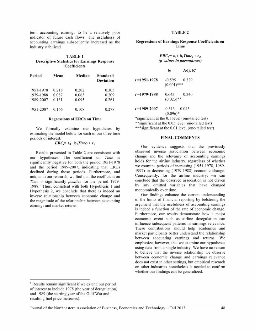
Journal of the Northeastern Association of Business, Economics and Technology—Fall 2013 48
term accounting earnings to be a relatively poor indicator of future cash flows. The usefulness of accounting earnings subsequently increased as the industry stabilized.
TABLE 1 Descriptive Statistics for Earnings Response
Coefficients Period Mean Median Standard Deviation
1951-1978 0.218 0.202 0.305 1979-1988 0.087 0.063 0.209 1989-2007 0.131 0.095 0.261 1951-2007 0.166 0.108 0.278
Regressions of ERCs on Time
We formally examine our hypotheses by
estimating the model below for each of our three time periods of interest:
ERCt= a0+ b1Timet + eit
Results presented in Table 2 are consistent with
our hypotheses. The coefficient on Time is significantly negative for both the period 1951-1978 and the period 1989-2007, indicating that ERCs declined during those periods. Furthermore, and unique to our research, we find that the coefficient on Time is significantly positive for the period 1979-1988.1 Thus, consistent with both Hypothesis 1 and Hypothesis 2, we conclude that there is indeed an inverse relationship between economic change and the magnitude of the relationship between accounting earnings and market returns.
1 Results remain significant if we extend our period of interest to include 1978 (the year of deregulation) and 1989 (the starting year of the Gulf War and resulting fuel price increases).
TABLE 2
Regressions of Earnings Response Coefficients on Time
ERCt = a0+ b1Timet + eit (p-values in parentheses)
b1 Adj. R2 t =1951-1978 -0.595 0.329 (0.001)*** t =1979-1988 0.643 0.340 (0.023)** t =1989-2007 -0.313 0.045 (0.096)* *significant at the 0.1 level (one-tailed test) **significant at the 0.05 level (one-tailed test) ***significant at the 0.01 level (one-tailed test)
FINAL COMMENTS
Our evidence suggests that the previously observed inverse association between economic change and the relevance of accounting earnings holds for the airline industry, regardless of whether we examine periods of increasing (1951-1978, 1989-1997) or decreasing (1979-1988) economic change. Consequently, for the airline industry, we can conclude that the observed association is not driven by any omitted variables that have changed monotonically over time.
Our findings enhance the current understanding of the limits of financial reporting by bolstering the argument that the usefulness of accounting earnings is indeed a function of the rate of economic change. Furthermore, our results demonstrate how a major economic event such as airline deregulation can influence subsequent patterns in earnings relevance. These contributions should help academics and market participants better understand the relationship between accounting earnings and returns. We emphasize, however, that we examine our hypotheses using data from a single industry. We have no reason to believe that the inverse relationship we observe between economic change and earnings relevance does not exist in other settings, but empirical research on other industries nonetheless is needed to confirm whether our findings can be generalized.
Journal of the Northeastern Association of Business, Economics and Technology—Fall 2013 49
REFERENCES American Institute of Certified Public Accountants
(AICPA) (1994). Improving Business Reporting: A Customer Focus. Report of the AICPA Special Committee on Financial Reporting ("Jenkins Committee"), New York: AICPA.
Bureau of Labor Statistics (2011). Career Guide to
Industries, 2010-2011 ed. Washington, DC: US Department of Labor.
Chow, C. and W. Van der Stede (2006). The Use and
Usefulness of Non-financial Performance Measures. Management Accounting Quarterly, 7, 10-15.
Collins, D.W., E.L. Maydew and I.S. Weiss (1997).
Changes in the Value-relevance of Earnings and Book Values Over the Past Forty Years. Journal of Accounting and Economics, 24(1), 39-67.
Federal Aviation Administration (2009). The
Economic Impact of Civil Aviation on the U.S. Economy. Washington, DC: Air Traffic Organization, FAA.
Grimm, C. and R. Windle (1998). Regulation and Deregulation in Surface Freight, Airlines and Telecommunications. Regulatory Reform and Labor Markets, J. Peoples, editor. Norwell, MA: Kluwer, 15-50.
Lev, B., and P. Zarowin (1999). The Boundaries of
Financial Reporting and How to Extend Them. Journal of Accounting Research, 37(2), 353-385.
Najda, C. (2003). Low-Cost Carriers and Low Fares:
Competition and Concentration in the US Airline Industry. Department of Economics, Stanford University, Stanford.
Office of Consumer Affairs (1988). Air Travel
Consumer Report. Washington, DC: US Department of Transportation.
Transportation Research Board (1990). Special
Report 226: Airport System Capacity: Strategic Choices. Washington, DC: National Research Council.
Wensveen, J.G. (2008). Air Transportation: A
Management Perspective, 6th ed. Aldershot, UK: Ashgate.
Stephen Liedtka, is an Associate Professor of Accounting at Villanova University. His research examines the relationship between accounting information and both business decision-making and firm value. During 2013, Professor Liedtka received the "Gerald A. Dougherty Endowed School of Business Faculty Award" from Villanova and an "Outstanding Author Contribution Award" from Emerald Publishing. Amy K. S. Scott, is an Associate Professor of Business at DeSales University. She teaches economics and finance courses in the undergraduate and MBA programs. Her research covers various areas including finance, corruption and the economic impact of sporting events. She is currently writing a managerial finance textbook for Flat World Knowledge.
Journal of the Northeastern Association of Business, Economics and Technology—Fall 2013 50
FROM SINGULAR TO GLOBAL, FROM PRIMAL TO DUAL: NEW USES FOR THE HERFINDAHL-HIRSCHMAN INDEX
Johnnie B. Linn III
ABSTRACT
The Herfindahl-Hirschman index, traditionally used to measure seller market power in a single industry, is expanded to cover a group of industries or the entire economy. Also, a global dual Herfindahl-Hirschman index is developed to measure concentration of uses of inputs across industries in an analogous way. The inverse of the global Herfindahl-Hirschman index is reinterpreted as the effective number of participants, rather than competitors only, as some can be complementary instead of competitive. Participants can be firms or entire industries. Manufacturing sector concentration data for about 300,000 firms in 2002 and 2007 yield a total of about 400 to 500 firms as effective participants across manufacturing. Make-use data for 69 industries from 1997 to 2012 show that there are about 36 effective primal producing industries and about 255 effective dual uses served by inputs.
INTRODUCTION The Herfindahl-Hirschman Index (HHI), or sum
of the squares of firms’ shares of sales of a good, measures the degree of competitiveness of firms selling that good. The HHI is used like a one-dimensional Pearson’s chi-square goodness of fit test: the greater the difference between the observed HHI and that which would be seen if all the firms had the same share of sales, the greater the degree of concentration for the good. The HHI is in fact equivalent to a one-dimensional Pearson’s chi-square test. As the Pearson’s chi square test can be expanded to measure across an additional dimension, the Herfindahl-Hirschman Index is here expanded to measure firms’ concentrations across different goods.
Adelman (1969) identified the inverse of the HHI as the number of effective competitors in a market. Here, the inverse is re-interpreted as the number of effective participants in a market. The more inclusive word “participants” encompasses the possibility of symbiotic relationships that can arise between firms when the extended HHI is developed.
Also, this paper shows how a dual HHI, or the degree of concentration of users of a particular input, can be extended across different inputs.
THE EQUIVALENCE OF THE HERFINDAHL-HIRSCHMAN INDEX AND THE PEARSON’S
CHI-SQUARE The equivalence of the HHI to a chi-square test
is seen in the initial exposition of the HHI in Hirschman (1945). Hirschman’s purpose in
proposing his new index is solve the problem that an index of mere concentration, such as the Gini coefficient, does not account for the degree of market power that arises from the fewness of the number of participants (p. 158).
The index as originally formulated by Hirschman is
where is the ith firm’s share of sales in a market with N firms. Herfindahl’s (1950) independent derivation of the index does not have the radical.
The Pearson’s chi-square goodness-of-fit test for N firms against maximum competitiveness is
where is the ith firm’s observed share of sales and 1/N is the expected value. The right hand side of Equation (2) appears in Hirschman’s first equation (p. 159) in the appendix of his book but is not specifically identified as a chi square. On expansion of the quadratic in Equation (2), we obtain
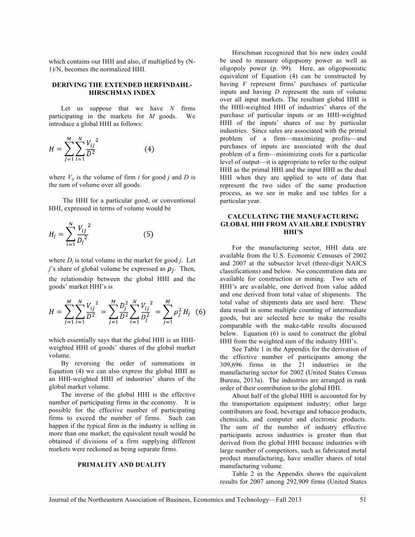
Journal of the Northeastern Association of Business, Economics and Technology—Fall 2013 51
which contains our HHI and also, if multiplied by (N-1)/N, becomes the normalized HHI.
DERIVING THE EXTENDED HERFINDAHL-
HIRSCHMAN INDEX Let us suppose that we have N firms
participating in the markets for M goods. We introduce a global HHI as follows:
where Vij is the volume of firm i for good j and D is the sum of volume over all goods.
The HHI for a particular good, or conventional HHI, expressed in terms of volume would be
where Dj is total volume in the market for good j. Let j’s share of global volume be expressed as . Then, the relationship between the global HHI and the goods’ market HHI’s is
which essentially says that the global HHI is an HHI-weighted HHI of goods’ shares of the global market volume.
By reversing the order of summations in Equation (4) we can also express the global HHI as an HHI-weighted HHI of industries’ shares of the global market volume.
The inverse of the global HHI is the effective number of participating firms in the economy. It is possible for the effective number of participating firms to exceed the number of firms. Such can happen if the typical firm in the industry is selling in more than one market; the equivalent result would be obtained if divisions of a firm supplying different markets were reckoned as being separate firms.
PRIMALITY AND DUALITY
Hirschman recognized that his new index could be used to measure oligopsony power as well as oligopoly power (p. 99). Here, an oligopsonistic equivalent of Equation (4) can be constructed by having V represent firms’ purchases of particular inputs and having D represent the sum of volume over all input markets. The resultant global HHI is the HHI-weighted HHI of industries’ shares of the purchase of particular inputs or an HHI-weighted HHI of the inputs’ shares of use by particular industries. Since sales are associated with the primal problem of a firm—maximizing profits—and purchases of inputs are associated with the dual problem of a firm—minimizing costs for a particular level of output—it is appropriate to refer to the output HHI as the primal HHI and the input HHI as the dual HHI when they are applied to sets of data that represent the two sides of the same production process, as we see in make and use tables for a particular year.
CALCULATING THE MANUFACTURING
GLOBAL HHI FROM AVAILABLE INDUSTRY HHI’S
For the manufacturing sector, HHI data are
available from the U.S. Economic Censuses of 2002 and 2007 at the subsector level (three-digit NAICS classifications) and below. No concentration data are available for construction or mining. Two sets of HHI’s are available, one derived from value added and one derived from total value of shipments. The total value of shipments data are used here. These data result in some multiple counting of intermediate goods, but are selected here to make the results comparable with the make-table results discussed below. Equation (6) is used to construct the global HHI from the weighted sum of the industry HHI’s.
See Table 1 in the Appendix for the derivation of the effective number of participants among the 309,696 firms in the 21 industries in the manufacturing sector for 2002 (United States Census Bureau, 2013a). The industries are arranged in rank order of their contribution to the global HHI.
About half of the global HHI is accounted for by the transportation equipment industry; other large contributors are food, beverage and tobacco products, chemicals, and computer and electronic products. The sum of the number of industry effective participants across industries is greater than that derived from the global HHI because industries with large number of competitors, such as fabricated metal product manufacturing, have smaller shares of total manufacturing volume.
Table 2 in the Appendix shows the equivalent results for 2007 among 292,909 firms (United States
Journal of the Northeastern Association of Business, Economics and Technology—Fall 2013 52
Census Bureau, 2013b). There are some changes in the ranking of the industries in their contribution to the global HHI. The most significant change is the increase in market share of petroleum and coal products manufacturing.
The number of effective firms is 439.0 in 2007 and 440.1 in 2012, indicating a high degree of concentration in the manufacturing sector at the firm level.
CALCULATING NATIONAL GLOBAL HHI’S
FROM MAKE-USE DATA With national make-use data, we can measure
concentration without the problem of the intermediation of firms. The U.S. Bureau of Economic Analysis releases summary data annually and detail and benchmark data at five-year intervals. The most recent available benchmark data are for 2007. At the detail level, benchmark data are broken out for 490 industries for 1997 (Bureau of Economic Analysis, 2002), 426 industries for 2002 (Bureau of Economic Analysis, 2013b) and 389 industries for 2007 (Bureau of Economic Analysis, 2014b). At the summary level, 2007 benchmark data are broken out for 69 industries. A “hybrid” set of summary benchmark data was broken out for 133 commodities for 2002 (Bureau of Economic Analysis, 2013a); this breakout was not repeated for 2007. For 2007, the benchmark data were integrated with the annual data; the benchmark tables for 2007 are also its annual tables. New sets of annual tables from 1997 to 2012 at the sector and summary levels were prepared to conform to the 2007 benchmark standards.
The make and use tables are available for commodities before redefinitions and commodities after redefinitions. The former are used for this study because they reflect the actual organization of production while the latter reassign for accounting purposes some commodities to industries that are the primary producers for those commodities.
The primal and dual global HHI’s can be calculated directly from Equation (4) but the 2007 and 2012 summary data will be shown below in the format of Equation (6) so that the industries and commodities that make the largest contributions to the global HHI’s can be extracted.
The commodities’ primal HHI’s are aggregated down columns of the summary make tables and weighted by the square of the commodities’ column totals’ shares of total output.
The industries’ dual HHI’s are aggregated down columns of the summary use tables and weighted by the square of the industries’ column totals’ shares of total intermediate use.
RESULTS FROM THE MAKE-USE DATA
The number of effective industries In Tables 3 and 4 in the Appendix, the top 25
commodities are ranked by their contribution to the global primal HHI in 2007 and 2012. The inverse of the global primal HHI is the number of effective industries in the economy.
Many commodities have high primal HHI’s because their respective industries are classified by what they make. An exception is miscellaneous professional, scientific, and technical services, which receives significant contributions from its off-diagonal elements in the make table. Hospitals have a significant off-diagonal contribution from state and local general government.
The top two leading contributors to the global primal HHI in 2007 and 2012 are real estate and state and local general government. Construction is a strong third in 2007 and falls to fifth place in 2012. Federal general government rises from a weak sixth place in 2007 to a level comparable to the top five commodities in 2012.
The number of effective industries is 35.9 in 2007 and 36.6 in 2012, roughly half of the 69 industries broken out at the summary level.
The number of effective uses
In Tables 5 and 6 in the Appendix, the top 25
industries are ranked by their contribution to the global dual HHI in 2007 and 2012. The inverse of the global dual HHI is the number of effective uses of commodities in the economy.
The industries’ dual HHI’s tend to be low because most have a number of upstream suppliers. A notable exception is petroleum and coal products, which is fed primarily from oil and gas extraction. The large contribution of insurance carriers and related activities arises from the large diagonal element for that industry, signifying interdependence. Funds, trusts, and other financial vehicles are fed primarily by the securities industry.
The top five industries—petroleum and coal product in particular--increased their shares of total intermediate use from 2002 to 2007. The contribution of petroleum and coal products to global dual HHI is sensitive to one off-diagonal element—Cell Z9—that represents the feed to it from oil and gas extraction.
The number of effective uses for commodities is 232 in 2007 and 196 in 2012, roughly three times the 69 commodities broken out at the summary level.
The annual data
Journal of the Northeastern Association of Business, Economics and Technology—Fall 2013 53
Table 7 in the Appendix shows the series of
effective number of commodities and the number of uses from 1997 to 2012 for the annual summary level tables. Included for comparison are the results for the 1997 benchmark detail tables (Bureau of Economic Analysis 2014a), the 2002 and 2007 benchmark detail tables, and the “hybrid” 2002 benchmark summary table.
The annual summary results from 1997 to 2012 show that the average primal ratio of effective industries to the total number of commodities is about one-half, and the average dual ratio of effective uses of commodities is about 3.7. Both series show a negative trend in the value of their ratios. The variation in the dual ratio is attributable largely to the variation in contribution of oil and gas extraction to petroleum and coal products.
The benchmark detail results exhibit effective numbers of industries and uses greater than those found at the summary level, but the ratios to their respective numbers of commodities are lower than at the summary level—about one seventh for the primal and about 1.5 for the dual. These lower ratios signify that at the detail level the disaggregation of commodities reduces the sensitivity of the findings to large values of individual cells in the tables. The results at the detail level support the conclusion that at the summary level, the degrees of concentration for the primal and dual results are significantly different.
IMPLICATIONS AND FURTHER WORK The results show that the conventional measure
of market concentration—the primal HHI—is not the whole story for the economy. The dual HHI shows that there is a high degree of diversification in the input markets.
The finding that the number of effective uses of commodities exceeds the number of commodities implies that the industries that serve these uses have diversified them to occupy niches in economic space, analogous to niches that individual species of animals and plants occupy in their environment. Hutchinson (1957) views a niche for an individual species of animal or plant as being embedded in a hypervolume of environmental factors affecting that species. Among those factors are other species that are present. Likewise, the niche occupied by an industry is partly defined by the other industries with which it interacts.
The finding that the number of effective industries and uses does not vary directly with the number of commodities indicates that the number of dimensions of space in which economic niches are embedded varies with the scale of measure,
analogous to how the volume occupied by the voids of a fractal changes as the level of its detail increases. What is suggested for further work, then, is to find fractals into which economic space can be embedded. The HHI concept can be used to find the number of “effective” voids in a fractal. The task, then, is to find fractals whose numbers of effective voids match the primal and dual values derived in this paper; then we can infer properties of the primal and dual spaces of the economy from the corresponding properties of the fractals.
REFERENCES
Adelman M.A. (1969). Comment on the ‘H’
concentration measure as a numbers equivalent. Review of Economics and Statistics, 51(February), 99–101.
Bureau of Economic Analysis (2002), A Preview of
the 1997 Benchmark Input-Output Accounts Retrieved (02/11/2014) from http://bea.gov/scb/pdf/2002/08August/0802_I-O_Benchmark.pdf
Bureau of Economic Analysis (2007), Integrating
the 2002 Benchmark Input-Output Accounts and the 2002 Annual Industry Accounts Retrieved (02/11/2014) from http://bea.gov/scb/pdf/2007/12%20December/1207_indyaccount.pdf
Bureau of Economic Analysis (2013a). Benchmark
Input-Output Data Retrieved (11/06/2013) from http://www.bea.gov/industry/xls/2002summary_makeuse.xls
Bureau of Economic Analysis (2013b). Benchmark
Input-Output Data Retrieved (11/06/2013) from http://www.bea.gov/industry/zip/2002detail.zip
Bureau of Economic Analysis (2014a), Benchmark
Input-Output Data, Retrieved (02/11/2014) from http://bea.gov/industry/io_benchmark.htm
Bureau of Economic Analysis (2014b), Input-Output
Accounts Data Retrieved (02/08/2014) from http://www.bea.gov/industry/io_annual.htm
Herfindahl, O.C. (1950). Concentration in the U.S.
Steel Industry (Unpublished doctoral dissertation). Columbia University, NY.
Hirschman, A.O. (1945). National power and the
structure of foreign trade. Berkeley: University of California Press.

Journal of the Northeastern Association of Business, Economics and Technology—Fall 2013 54
Hutchinson, G.E. (1957). Concluding remarks. Cold
Spring Harbor Symposium on Quantitative Biology, 22, 415-457.
United States Census Bureau (2013a). EC0231SR12 -
Manufacturing: Subject Series - Concentration Ratios: Share of Value of Shipments Accounted for by the 4, 8, 20, and 50 Largest Companies for Industries Retrieved (11/09/2013) from http://factfinder2.census.gov/faces/tableservices/jsf/pages/productview.xhtml?pid=ECN_2002_US_31SR12&prodType=table
United States Census Bureau (2013b). EC0731SR12
- EC0731SR2: Manufacturing: Subject Series: Concentration Ratios: Share of Value of Shipments Accounted for by the 4, 8, 20, and 50 Largest Companies for Industries Retrieved (11/06/2013) from http://factfinder2.census.gov/faces/tableservices/jsf/pages/productview.xhtml?pid=ECN_2007_US_31SR12&prodType=table
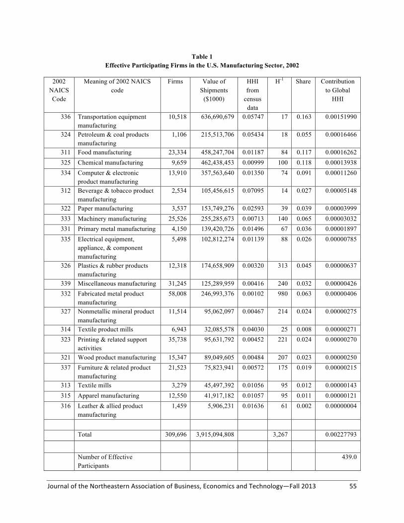
Journal of the Northeastern Association of Business, Economics and Technology—Fall 2013 55
Table 1 Effective Participating Firms in the U.S. Manufacturing Sector, 2002
2002
NAICS Code
Meaning of 2002 NAICS code
Firms Value of Shipments
($1000)
HHI from
census data
H-1 Share Contribution to Global
HHI
336 Transportation equipment manufacturing
10,518 636,690,679 0.05747 17 0.163 0.00151990
324 Petroleum & coal products manufacturing
1,106 215,513,706 0.05434 18 0.055 0.00016466
311 Food manufacturing 23,334 458,247,704 0.01187 84 0.117 0.00016262 325 Chemical manufacturing 9,659 462,438,453 0.00999 100 0.118 0.00013938 334 Computer & electronic
product manufacturing 13,910 357,563,640 0.01350 74 0.091 0.00011260
312 Beverage & tobacco product manufacturing
2,534 105,456,615 0.07095 14 0.027 0.00005148
322 Paper manufacturing 3,537 153,749,276 0.02593 39 0.039 0.00003999 333 Machinery manufacturing 25,526 255,285,673 0.00713 140 0.065 0.00003032 331 Primary metal manufacturing 4,150 139,420,726 0.01496 67 0.036 0.00001897 335 Electrical equipment,
appliance, & component manufacturing
5,498 102,812,274 0.01139 88 0.026 0.00000785
326 Plastics & rubber products manufacturing
12,318 174,658,909 0.00320 313 0.045 0.00000637
339 Miscellaneous manufacturing 31,245 125,289,959 0.00416 240 0.032 0.00000426 332 Fabricated metal product
manufacturing 58,008 246,993,376 0.00102 980 0.063 0.00000406
327 Nonmetallic mineral product manufacturing
11,514 95,062,097 0.00467 214 0.024 0.00000275
314 Textile product mills 6,943 32,085,578 0.04030 25 0.008 0.00000271 323 Printing & related support
activities 35,738 95,631,792 0.00452 221 0.024 0.00000270
321 Wood product manufacturing 15,347 89,049,605 0.00484 207 0.023 0.00000250 337 Furniture & related product
manufacturing 21,523 75,823,941 0.00572 175 0.019 0.00000215
313 Textile mills 3,279 45,497,392 0.01056 95 0.012 0.00000143 315 Apparel manufacturing 12,550 41,917,182 0.01057 95 0.011 0.00000121 316 Leather & allied product
manufacturing 1,459 5,906,231 0.01636 61 0.002 0.00000004
Total 309,696 3,915,094,808 3,267 0.00227793
Number of Effective Participants
439.0
Journal of the Northeastern Association of Business, Economics and Technology—Fall 2013 56
Table 2 Effective Participating Firms in the U.S. Manufacturing Sector, 2007
2007
NAICS Code
Meaning of 2007 NAICS Code
Firms Total value of shipments ($1,000)
HHI from
census data
H-1 Share Contribution to Global
HHI
324 Petroleum and coal products manufacturing
1,097 615,484,030 0.07347 14 0.116 0.00098358
336 Transportation equipment manufacturing
10,896 745,947,384 0.03650 27 0.140 0.00071775
325 Chemical manufacturing 10,060 716,152,473 0.01140 88 0.135 0.00020662 311 Food manufacturing 21,355 589,725,614 0.01021 98 0.111 0.00012548 334 Computer and electronic
product manufacturing 12,836 395,728,996 0.01366 73 0.074 0.00007560
331 Primary metal manufacturing 3,746 256,851,055 0.01806 55 0.048 0.00004211 312 Beverage and tobacco
product manufacturing 3,232 128,130,807 0.05554 18 0.024 0.00003222
333 Machinery manufacturing 23,989 350,499,485 0.00727 138 0.066 0.00003156 322 Paper manufacturing 3,242 176,687,641 0.02278 44 0.033 0.00002513 335 Electrical equipment,
appliance, and component manufacturing
5,400 129,180,071 0.01053 95 0.024 0.00000621
327 Nonmetallic mineral product manufacturing
11,462 127,978,584 0.00896 112 0.024 0.00000519
326 Plastics and rubber products manufacturing
11,322 209,335,541 0.00313 319 0.039 0.00000485
339 Miscellaneous manufacturing 30,934 148,913,381 0.00524 191 0.028 0.00000411 332 Fabricated metal product
manufacturing 56,808 345,166,675 0.00090 1111 0.065 0.00000379
323 Printing and related support activities
32,187 103,018,470 0.00779 128 0.019 0.00000292
337 Furniture and related product manufacturing
20,926 85,049,179 0.00615 163 0.016 0.00000157
321 Wood product manufacturing 14,817 101,711,917 0.00383 261 0.019 0.00000140 314 Textile product mills 6,433 28,682,164 0.04186 24 0.005 0.00000122 313 Textile mills 2,562 36,130,750 0.01602 62 0.007 0.00000074 315 Apparel manufacturing 8,346 23,626,238 0.00440 227 0.004 0.00000009 316 Leather and allied product
manufacturing 1,259 5,455,857 0.01748 57 0.001 0.00000002
Total 292,909 5,319,456,312 3,306 0.00227216 Number of Effective
Participants 440.1
Journal of the Northeastern Association of Business, Economics and Technology—Fall 2013 57
Table 3
Make Concentration by Commodity, Summary Data, 2007 Commodity
Code Commodity Total
Commodity Output
Commodity Primal HHI
Commodity Share of Output
Contribution to Global
HHI 531 Real estate 2,378,567 0.9727 0.00827 0.008043
GSLG State and local general government 1,411,371 1.0000 0.00291 0.002911 23 Construction 1,428,239 0.8666 0.00298 0.002584 42 Wholesale trade 1,243,950 0.8967 0.00226 0.002028
5412OP Miscellaneous professional, scientific, and technical services 1,431,104 0.4773 0.00299 0.001429
GFG Federal general government 798,350 1.0000 0.00093 0.000932
311FT Food and beverage and tobacco products 721,882 0.9515 0.00076 0.000725
621 Ambulatory health care services 723,413 0.9341 0.00076 0.000714
524 Insurance carriers and related activities 701,448 0.9860 0.00072 0.000709
4A0 Other retail 718,791 0.8993 0.00076 0.000679 325 Chemical products 712,370 0.8790 0.00074 0.000652
521CI Federal Reserve banks, credit intermediation, and related activities 658,144 0.9257 0.00063 0.000586
561 Administrative and support services 586,852 0.9505 0.00050 0.000478 324 Petroleum and coal products 589,439 0.9258 0.00051 0.000470
513 Broadcasting and telecommunications 555,344 0.9984 0.00045 0.000450
622 Hospitals 649,521 0.6748 0.00062 0.000416 81 Other services, except government 667,115 0.6282 0.00065 0.000409
722 Food services and drinking places 611,661 0.6953 0.00055 0.000380
3361MV Motor vehicles, bodies and trailers, and parts 498,082 0.9869 0.00036 0.000358
523 Securities, commodity contracts, and investments 522,389 0.8365 0.00040 0.000334
22 Utilities 529,855 0.6913 0.00041 0.000284
55 Management of companies and enterprises 420,440 1.0000 0.00026 0.000258
334 Computer and electronic products 380,246 0.9627 0.00021 0.000203 333 Machinery 334,475 0.9239 0.00016 0.000151 332 Fabricated metal products 330,829 0.9354 0.00016 0.000150
All Others 6,553,365
0.001545 Total 26,157,242
0.027878
Number of Effective Industries 35.9
Journal of the Northeastern Association of Business, Economics and Technology—Fall 2013 58
Table 4
Make Concentration by Commodity, Summary Data, 2012 Commodity
Code Commodity Total
Commodity Output
Commodity Primal HHI
Commodity Share of Output
Contribution to Global
HHI 531 Real estate 2,559,266 0.9687 0.00796 0.007706
GSLG State and local general government 1,536,356 1.0000 0.00287 0.002867 42 Wholesale trade 1,379,577 0.9052 0.00231 0.002093
5412OP Miscellaneous professional, scientific, and technical services 1,563,197 0.5031 0.00297 0.001493
23 Construction 1,148,259 0.8616 0.00160 0.001380 GFG Federal general government 1,011,673 1.0000 0.00124 0.001243
311FT Food and beverage and tobacco products 891,493 0.9529 0.00097 0.000920
621 Ambulatory health care services 885,485 0.9324 0.00095 0.000888 324 Petroleum and coal products 817,136 0.9195 0.00081 0.000746
524 Insurance carriers and related activities 774,667 0.9839 0.00073 0.000717
4A0 Other retail 782,353 0.8954 0.00074 0.000666 325 Chemical products 782,469 0.8840 0.00074 0.000657 622 Hospitals 850,452 0.6781 0.00088 0.000596
513 Broadcasting and telecommunications 649,449 0.9984 0.00051 0.000511
561 Administrative and support services 660,070 0.9484 0.00053 0.000502 722 Food services and drinking places 723,542 0.7019 0.00064 0.000446
81 Other services, except government 722,383 0.6310 0.00063 0.000400
521CI Federal Reserve banks, credit intermediation, and related activities 589,209 0.9385 0.00042 0.000396
55 Management of companies and enterprises 517,137 1.0000 0.00032 0.000325
3361MV Motor vehicles, bodies and trailers, and parts 516,592 0.9890 0.00032 0.000321
523 Securities, commodity contracts, and investments 463,073 0.8180 0.00026 0.000213
111CA Farms 389,600 0.9962 0.00018 0.000184 22 Utilities 491,082 0.6199 0.00029 0.000182
333 Machinery 384,547 0.9119 0.00018 0.000164 334 Computer and electronic products 328,331 0.9492 0.00013 0.000124
All Others 7,276,067
0.001605 Total 28,693,465
0.027344
Number of Effective Industries 36.6
Journal of the Northeastern Association of Business, Economics and Technology—Fall 2013 59
Table 5
Use Concentration by Industry, Summary Data, 2007
Industry Code
Industry Total Intermediate
Use
Industry Dual HHI
Industry Share of
Intermediate Use
Contribu-tion to Global
Dual HHI 324 Petroleum and coal products 447,019 0.7160 0.03828 0.0010493 531 Real estate 707,319 0.1036 0.06057 0.0003802 325 Chemical products 451,179 0.2504 0.03864 0.0003738
311FT Food and beverage and tobacco products 521,138 0.1837 0.04463 0.0003659
524 Insurance carriers and related activities 310,872 0.4736 0.02662 0.0003357
3361MV Motor vehicles, bodies and trailers, and parts 388,163 0.1851 0.03324 0.0002046
23 Construction 614,264 0.0670 0.05260 0.0001855
5412OP Miscellaneous professional, scientific, and technical services 420,183 0.1159 0.03598 0.0001500
GSLG State and local general government 577,798 0.0509 0.04948 0.0001246
521CI Federal Reserve banks, credit intermediation, and related activities 317,396 0.1476 0.02718 0.0001091
513 Broadcasting and telecommunications 274,805 0.1573 0.02353 0.0000871
42 Wholesale trade 408,484 0.0682 0.03498 0.0000834
523 Securities, commodity contracts, and investments 317,675 0.0943 0.02721 0.0000698
332 Fabricated metal products 205,959 0.1895 0.01764 0.0000590 4A0 Other retail 263,428 0.1033 0.02256 0.0000526 331 Primary metals 190,825 0.1959 0.01634 0.0000523
GFG Federal general government 302,282 0.0773 0.02589 0.0000518 334 Computer and electronic products 203,847 0.1614 0.01746 0.0000492
22 Utilities 203,096 0.1475 0.01739 0.0000446 621 Ambulatory health care services 267,417 0.0775 0.02290 0.0000406 722 Food services and drinking places 242,580 0.0937 0.02077 0.0000404
525 Funds, trusts, and other financial vehicles 74,884 0.8304 0.00641 0.0000342
326 Plastics and rubber products 141,559 0.2077 0.01212 0.0000305 333 Machinery 215,455 0.0895 0.01845 0.0000305
111CA Farms 188,860 0.1071 0.01617 0.0000280 All Others 3,420,443
0.0002732
Total 11,676,930
0.0043059
Number of Effective Uses 232.2
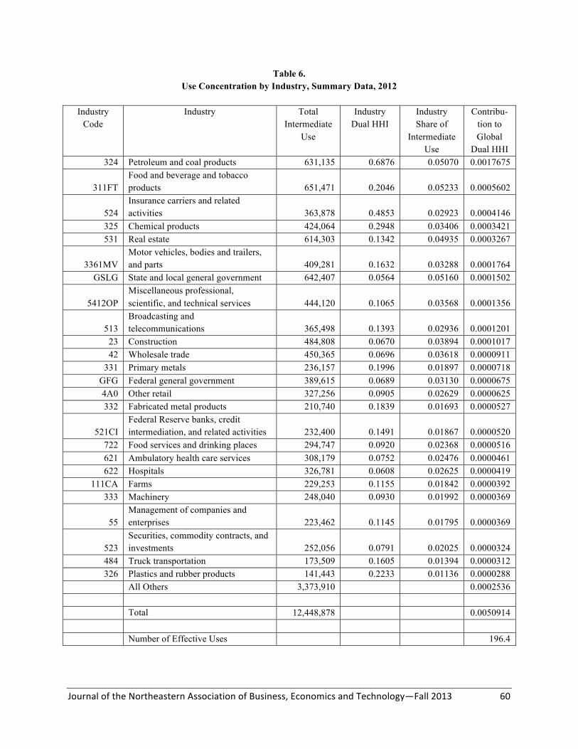
Journal of the Northeastern Association of Business, Economics and Technology—Fall 2013 60
Table 6. Use Concentration by Industry, Summary Data, 2012
Industry
Code Industry Total
Intermediate Use
Industry Dual HHI
Industry Share of
Intermediate Use
Contribu-tion to Global
Dual HHI 324 Petroleum and coal products 631,135 0.6876 0.05070 0.0017675
311FT Food and beverage and tobacco products 651,471 0.2046 0.05233 0.0005602
524 Insurance carriers and related activities 363,878 0.4853 0.02923 0.0004146
325 Chemical products 424,064 0.2948 0.03406 0.0003421 531 Real estate 614,303 0.1342 0.04935 0.0003267
3361MV Motor vehicles, bodies and trailers, and parts 409,281 0.1632 0.03288 0.0001764
GSLG State and local general government 642,407 0.0564 0.05160 0.0001502
5412OP Miscellaneous professional, scientific, and technical services 444,120 0.1065 0.03568 0.0001356
513 Broadcasting and telecommunications 365,498 0.1393 0.02936 0.0001201
23 Construction 484,808 0.0670 0.03894 0.0001017 42 Wholesale trade 450,365 0.0696 0.03618 0.0000911
331 Primary metals 236,157 0.1996 0.01897 0.0000718 GFG Federal general government 389,615 0.0689 0.03130 0.0000675 4A0 Other retail 327,256 0.0905 0.02629 0.0000625 332 Fabricated metal products 210,740 0.1839 0.01693 0.0000527
521CI Federal Reserve banks, credit intermediation, and related activities 232,400 0.1491 0.01867 0.0000520
722 Food services and drinking places 294,747 0.0920 0.02368 0.0000516 621 Ambulatory health care services 308,179 0.0752 0.02476 0.0000461 622 Hospitals 326,781 0.0608 0.02625 0.0000419
111CA Farms 229,253 0.1155 0.01842 0.0000392 333 Machinery 248,040 0.0930 0.01992 0.0000369
55 Management of companies and enterprises 223,462 0.1145 0.01795 0.0000369
523 Securities, commodity contracts, and investments 252,056 0.0791 0.02025 0.0000324
484 Truck transportation 173,509 0.1605 0.01394 0.0000312 326 Plastics and rubber products 141,443 0.2233 0.01136 0.0000288
All Others 3,373,910
0.0002536 Total 12,448,878
0.0050914
Number of Effective Uses 196.4
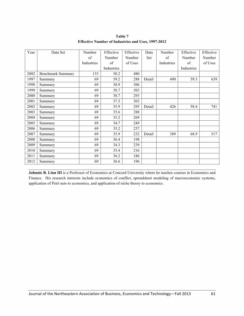
Journal of the Northeastern Association of Business, Economics and Technology—Fall 2013 61
Table 7
Effective Number of Industries and Uses, 1997-2012
Year Data Set Number of
Industries
Effective Number
of Industries
Effective Number of Uses
Data Set
Number of
Industries
Effective Number
of Industries
Effective Number of Uses
2002 Benchmark Summary 133 50.2 480 1997 Summary 69 39.2 288 Detail 490 59.3 639 1998 Summary 69 38.9 306 1999 Summary 69 38.7 303 2000 Summary 69 38.7 293 2001 Summary 69 37.3 303 2002 Summary 69 35.9 295 Detail 426 58.4 741 2003 Summary 69 35.6 288 2004 Summary 69 35.2 269 2005 Summary 69 34.7 249 2006 Summary 69 35.2 237 2007 Summary 69 35.9 232 Detail 389 68.9 517 2008 Summary 69 36.4 198 2009 Summary 69 34.3 239 2010 Summary 69 35.4 216 2011 Summary 69 36.2 186 2012 Summary 69 36.6 196 Johnnie B. Linn III is a Professor of Economics at Concord University where he teaches courses in Economics and Finance. His research interests include economics of conflict, spreadsheet modeling of macroeconomic systems, application of Petri nets to economics, and application of niche theory to economics.
Journal of the Northeastern Association of Business, Economics and Technology—Fall 2013 62
DEAL MAKING IN PAWN STARS: TESTING THEORIES OF BARGAINING
Bryan C. McCannon and John B. Stevens
_____________________________________________________________________________________________
ABSTRACT
Management and economic theories of negotiations are tested using a unique data set. The History Channel television show Pawn Stars portrays many negotiations between customers and workers at a pawn shop. This provides a unique data set not typically available to researchers as the tactics of bargaining can be observed, recorded, and analyzed. The use of experts, experience, the gap between the initial offers, and the use of final offers all affect the likelihood of a deal being made as well as the division of the surplus. The party making the opening offer suffers a disadvantage, which stands in contrast to predictions of sequential bargaining and anchoring effects.
_____________________________________________________________________________________________
INTRODUCTION
Bargaining is an essential activity of managerial decisionmaking. Whether it be negotiating with organized labor, interactions along the supply chain, or deal making with retailers, bargaining is a common activity in organizations. Consequently, the fields of management and economics have devoted significant attention to developing theories regarding the functioning of bargaining situations. Numerous theories have been developed to understand when bilateral bargaining is successful and when it may fail. Few have empirically tested the developed theories.
To conduct a formal and rigorous investigation into these theories, one needs data that allows for hypotheses derived from these theories to be tested. The primary limitation faced by researchers is that the data is typically unavailable. There is simply no one recording the bargaining process to create a data set.
To fill this void case studies and laboratory experiments have been conducted. Researchers such as van Poucke and Buelens (2002), Kristensen and Gärling (1997, 2000), Galinsky, Seiden, Kim, and Medvec(2002), and Zwick and Chen (1999) have created hypothetical bargaining situations in the lab. Along with being able to create data to analyze, these researchers are able to control the environment to study how changes in it affect the ability to make a deal. Examples of environmental adjustments include changing the sequencing of offer-making, adjusting reservation values, and providing suggestion prices which may serve as anchors in the negotiation. While such efforts are extremely valuable, they are exposed to the criticism that decisionmaking in the laboratory is artificial and bears little resemblance to real-world
behavior. Not only are these choices unique, but it has been shown, in field studies of deal making over time (List and Millimet, 2008), that behaviors adjust as individuals gain experience engaging in market behavior.
The television show Pawn Stars provides a unique opportunity to address this shortcoming and formally test theories in management science and economics. The reality show airs actual negotiations between agents of a pawn store and customers who bring in items to sell. Typically, interesting and unique items, without readily available information on resale market prices, are negotiated over. The show depicts the entire transaction with the initial offers, counteroffers, bargaining tactics, and use of third-party experts. Furthermore, since there have been multiple seasons, a large data set of these transactions is available. Our objective is to provide a rigorous empirical test of many popular theories of negotiation using this unique data set.
We first outline three major categories of impediments to the bargaining process. The relevant theories in management science and economics are described. Then, we describe the data collected from the television show and conduct an analysis of how measureable factors of the negotiating process relate to the frequency of deals successfully being made. Finally, a formal econometric analysis of how all of the measureable characteristics of the bargaining process affect the probability of a deal being made is conducted.
We find evidence supporting the theories commonly discussed in management and economics. It is shown that the tactic of using final offers, where one party creates a take-it-or-leave-it offer, greatly improves the chances of a deal being made. The experience and fluidity of the participants correlates
Journal of the Northeastern Association of Business, Economics and Technology—Fall 2013 63
well with success at the bargaining table. Finally, theories regarding the impact of asymmetric information and expertise find some empirical support.
PROMINENT THEORIES OF BARGAINING
Economics and management science has articulated a number of important theories related to successful deal making. In what follows, we summarize, as briefly as possible without losing too much clarity, some of the most prominent theories that can be related to our available data. Asymmetric Information A basic presupposition in microeconomic theory is that trade, absent negative externalities, creates mutual gain. Put simply, parties to any trade agree to the trade because they believe they benefit more than they lose. In economics, such a mutual welfare improvement is referred to as a Pareto Improvement. One way for a negotiation to fail is if there exists no mutually advantageous outcome. In this situation it actual expands economic welfare for bargaining to fail. The question arises, though, does the reverse hold? Supposing there actually exists a mutually beneficial trade, is it necessarily true that bargaining between two parties will arrive at it? It is generally presumed that the answer is no. There exist environments in which some restriction or constraint stands in the way of arriving at Pareto Improvements. The most prominent of the theories of market failure arises from the research of Akerlof (1970). He illustrated that asymmetric information provides the opportunity for failed beneficial deal making. If one side of a transaction is endowed with superior information, then the other party is left with a strategic disadvantage. For example, if the seller of the item has solid information that the item is authentic, rare, and would command a high price in resale markets (but there is a constraint prohibiting him from taking advantage of it), the poorly-informed buyer is uncertain whether he/she is negotiating with someone selling such an item or interacting with a seller who knows that the item is not authentic or simply would not command much demand in secondary markets. Fearful of the latter he/she would be unwilling to pay a high price for the good and the potential arises for failed negotiations, not because of negative gains from trade, but because of the poor information. What is important for the market failure is not just that there exists incomplete information, but that the information is lop-sided.
How do markets deal with the unraveling due to asymmetric information? While there are numerous possibilities, one important way is to directly collect some of the unknown information. A third-party, disinterested expert can be employed to improve the informational imperfections. Experts can provide not only improved information, but symmetric information. This can, then, alleviate the concern in situations such as the hypothetical one previously described, and result in successful deal making. Examples of real-world, third-party experts would be CarFax reports on vehicle history and appraisals of homes, jewelry, coins, etc. In the television show Pawn Stars third-party experts are frequently brought in to provide information on authenticity, rarity, background information, and auction-market price. The use of third-party experts, especially those who appraise items, has been shown to have a important impacts on markets. For example, McCannon (2012) illustrates that the price of cigars not only correlates with expert evaluations of prices, but as more informed information is aggregated, the predictive power of the evaluation improves. Final Offers Another important theory of success in deal making is the use of final offers. Schelling’s (1960) seminal work investigates strategies and tactics employed in situations of conflicts. While the focus of this Nobel Prize-winning work is on military conflict and nuclear arms races, the theoretical arguments made can be applied to bargaining. A primary point of his work is the emphasis in the value of take-it-or-leave-it offers. Schelling argued that if a party to the conflict (i.e. negotiation) is able to frame the situation to one where the other party is left with a binary decision to accept the offer or reject it receiving only her default/outside option, then the demanding party fares well. The success of final offers depends critically on the ability to convince the recipient of the offer that it is, indeed, a final offer. Hence, one would expect that the use of final offers would be both correlated with the likelihood of a deal being made and the amount of surplus captured by the party making the final offer. Experience It is also argued that experience in trading should matter for the ability to successfully complete a deal. As an example, Knetsch and Sinden (1984) illustrate, in an experimental setting, that individuals experience a bias towards one’s status quo endowment. Individuals endowed with one particular
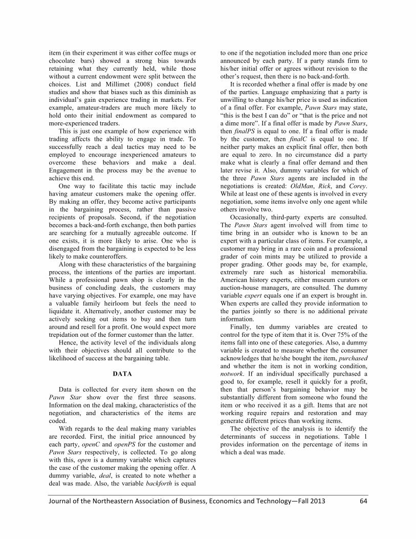
Journal of the Northeastern Association of Business, Economics and Technology—Fall 2013 64
item (in their experiment it was either coffee mugs or chocolate bars) showed a strong bias towards retaining what they currently held, while those without a current endowment were split between the choices. List and Millimet (2008) conduct field studies and show that biases such as this diminish as individual’s gain experience trading in markets. For example, amateur-traders are much more likely to hold onto their initial endowment as compared to more-experienced traders. This is just one example of how experience with trading affects the ability to engage in trade. To successfully reach a deal tactics may need to be employed to encourage inexperienced amateurs to overcome these behaviors and make a deal. Engagement in the process may be the avenue to achieve this end. One way to facilitate this tactic may include having amateur customers make the opening offer. By making an offer, they become active participants in the bargaining process, rather than passive recipients of proposals. Second, if the negotiation becomes a back-and-forth exchange, then both parties are searching for a mutually agreeable outcome. If one exists, it is more likely to arise. One who is disengaged from the bargaining is expected to be less likely to make counteroffers. Along with these characteristics of the bargaining process, the intentions of the parties are important. While a professional pawn shop is clearly in the business of concluding deals, the customers may have varying objectives. For example, one may have a valuable family heirloom but feels the need to liquidate it. Alternatively, another customer may be actively seeking out items to buy and then turn around and resell for a profit. One would expect more trepidation out of the former customer than the latter. Hence, the activity level of the individuals along with their objectives should all contribute to the likelihood of success at the bargaining table.
DATA
Data is collected for every item shown on the Pawn Star show over the first three seasons. Information on the deal making, characteristics of the negotiation, and characteristics of the items are coded.
With regards to the deal making many variables are recorded. First, the initial price announced by each party, openC and openPS for the customer and Pawn Stars respectively, is collected. To go along with this, open is a dummy variable which captures the case of the customer making the opening offer. A dummy variable, deal, is created to note whether a deal was made. Also, the variable backforth is equal
to one if the negotiation included more than one price announced by each party. If a party stands firm to his/her initial offer or agrees without revision to the other’s request, then there is no back-and-forth.
It is recorded whether a final offer is made by one of the parties. Language emphasizing that a party is unwilling to change his/her price is used as indication of a final offer. For example, Pawn Stars may state, “this is the best I can do” or “that is the price and not a dime more”. If a final offer is made by Pawn Stars, then finalPS is equal to one. If a final offer is made by the customer, then finalC is equal to one. If neither party makes an explicit final offer, then both are equal to zero. In no circumstance did a party make what is clearly a final offer demand and then later revise it. Also, dummy variables for which of the three Pawn Stars agents are included in the negotiations is created: OldMan, Rick, and Corey. While at least one of these agents is involved in every negotiation, some items involve only one agent while others involve two.
Occasionally, third-party experts are consulted. The Pawn Stars agent involved will from time to time bring in an outsider who is known to be an expert with a particular class of items. For example, a customer may bring in a rare coin and a professional grader of coin mints may be utilized to provide a proper grading. Other goods may be, for example, extremely rare such as historical memorabilia. American history experts, either museum curators or auction-house managers, are consulted. The dummy variable expert equals one if an expert is brought in. When experts are called they provide information to the parties jointly so there is no additional private information.
Finally, ten dummy variables are created to control for the type of item that it is. Over 75% of the items fall into one of these categories. Also, a dummy variable is created to measure whether the consumer acknowledges that he/she bought the item, purchased and whether the item is not in working condition, notwork. If an individual specifically purchased a good to, for example, resell it quickly for a profit, then that person’s bargaining behavior may be substantially different from someone who found the item or who received it as a gift. Items that are not working require repairs and restoration and may generate different prices than working items. The objective of the analysis is to identify the determinants of success in negotiations. Table 1 provides information on the percentage of items in which a deal was made.
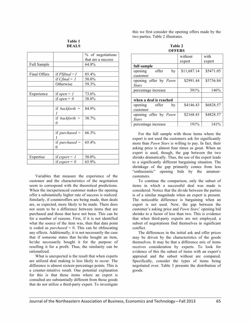
Journal of the Northeastern Association of Business, Economics and Technology—Fall 2013 65
Table 1 DEALS
Variables that measure the experience of the customer and the characteristics of the negotiation seem to correspond with the theoretical predictions. When the inexperienced customer makes the opening offer a substantially higher rate of success is realized. Similarly, if counteroffers are being made, then deals are, as expected, more likely to be made. There does not seem to be a difference between items that are purchased and those that have not been. This can be for a number of reasons. First, if it is not identified what the source of the item was, then that data point is coded as purchased = 0. This can be obfuscating any effects. Additionally, it is not necessarily the case that if someone states that he/she bought an item, he/she necessarily bought it for the purpose of reselling it for a profit. Thus, the similarity can be rationalized. What is unexpected is the result that when experts are utilized deal making is less likely to occur. The difference is almost sixteen percentage points. This is a counter-intuitive result. One potential explanation for this is that those items where an expert is consulted are substantially different from those goods that do not utilize a third-party expert. To investigate
this we first consider the opening offers made by the two parties. Table 2 illustrates.
Table 2
OFFERS
For the full sample with those items where the
expert is not used the customers ask for significantly more than Pawn Stars is willing to pay. In fact, their asking price is almost four times as great. When an expert is used, though, the gap between the two shrinks dramatically. Thus, the use of the expert leads to a significantly different bargaining situation. The shrinkage of the gap primarily comes from less “enthusiastic” opening bids by the amateur-customers.
To continue the comparison, only the subset of items in which a successful deal was made is considered. Notice that the divide between the parties is of a similar magnitude when an expert is present. The noticeable difference is bargaining when an expert is not used. Now, the gap between the customer’s asking price and Pawn Stars’ opening bid shrinks to a factor of less than two. This is evidence that when third-party experts are not employed, a subset of negotiations find themselves in significant conflict.
The differences in the initial ask and offer prices may be driven by the characteristics of the goods themselves. It may be that a difference mix of items receives consideration by experts. To look for evidence of this the subset of items with an expert’s appraisal and the subset without are compared. Specifically, consider the types of items being negotiated over. Table 3 presents the distribution of goods.
% of negotiations that are a success
Full Sample 64.8% Final Offers if PSfinal =1 85.4% if Cfinal = 1 50.0% Otherwise 59.3% Experience if open = 1 73.6% if open = 0 38.8% if backforth =
1 84.9%
if backforth = 0
38.7%
if purchased =
1 66.3%
if purchased = 0
65.4%
Expertise if expert = 1 50.0% if expert = 0 65.9%
without expert
with expert
full sample opening offer by customer
$11,687.14 $5471.05
opening offer by Pawn Stars
$2991.44 $3736.84
percentage increase 391% 146% when a deal is reached opening offer by customer
$4146.43 $6828.57
opening offer by Pawn Stars
$2168.43 $4828.57
percentage increase 191% 141%
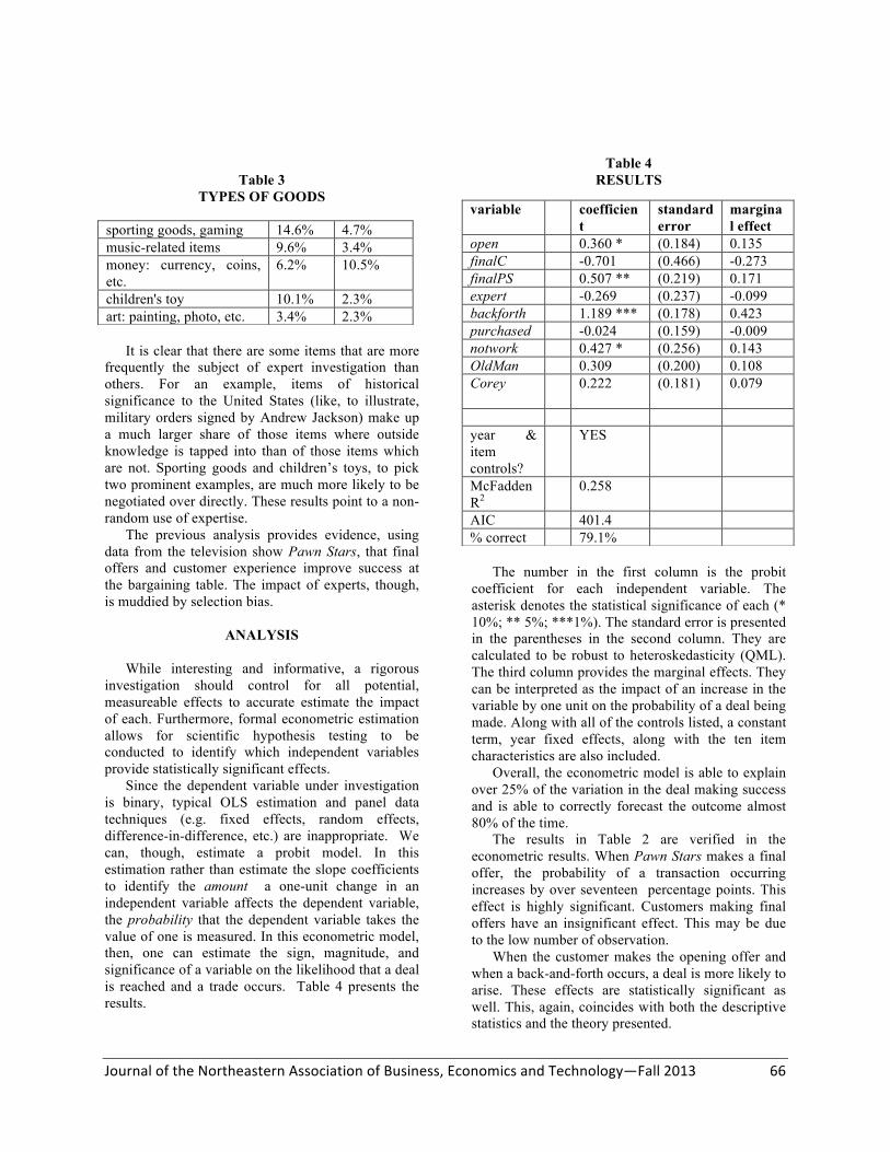
Journal of the Northeastern Association of Business, Economics and Technology—Fall 2013 66
Table 3 TYPES OF GOODS
It is clear that there are some items that are more frequently the subject of expert investigation than others. For an example, items of historical significance to the United States (like, to illustrate, military orders signed by Andrew Jackson) make up a much larger share of those items where outside knowledge is tapped into than of those items which are not. Sporting goods and children’s toys, to pick two prominent examples, are much more likely to be negotiated over directly. These results point to a non-random use of expertise. The previous analysis provides evidence, using data from the television show Pawn Stars, that final offers and customer experience improve success at the bargaining table. The impact of experts, though, is muddied by selection bias.
ANALYSIS While interesting and informative, a rigorous investigation should control for all potential, measureable effects to accurate estimate the impact of each. Furthermore, formal econometric estimation allows for scientific hypothesis testing to be conducted to identify which independent variables provide statistically significant effects. Since the dependent variable under investigation is binary, typical OLS estimation and panel data techniques (e.g. fixed effects, random effects, difference-in-difference, etc.) are inappropriate. We can, though, estimate a probit model. In this estimation rather than estimate the slope coefficients to identify the amount a one-unit change in an independent variable affects the dependent variable, the probability that the dependent variable takes the value of one is measured. In this econometric model, then, one can estimate the sign, magnitude, and significance of a variable on the likelihood that a deal is reached and a trade occurs. Table 4 presents the results.
Table 4 RESULTS
The number in the first column is the probit coefficient for each independent variable. The asterisk denotes the statistical significance of each (* 10%; ** 5%; ***1%). The standard error is presented in the parentheses in the second column. They are calculated to be robust to heteroskedasticity (QML). The third column provides the marginal effects. They can be interpreted as the impact of an increase in the variable by one unit on the probability of a deal being made. Along with all of the controls listed, a constant term, year fixed effects, along with the ten item characteristics are also included. Overall, the econometric model is able to explain over 25% of the variation in the deal making success and is able to correctly forecast the outcome almost 80% of the time. The results in Table 2 are verified in the econometric results. When Pawn Stars makes a final offer, the probability of a transaction occurring increases by over seventeen percentage points. This effect is highly significant. Customers making final offers have an insignificant effect. This may be due to the low number of observation. When the customer makes the opening offer and when a back-and-forth occurs, a deal is more likely to arise. These effects are statistically significant as well. This, again, coincides with both the descriptive statistics and the theory presented.
sporting goods, gaming 14.6% 4.7% music-related items 9.6% 3.4% money: currency, coins, etc.
6.2% 10.5%
children's toy 10.1% 2.3% art: painting, photo, etc. 3.4% 2.3%
variable coefficient
standard error
marginal effect
open 0.360 * (0.184) 0.135 finalC -0.701 (0.466) -0.273 finalPS 0.507 ** (0.219) 0.171 expert -0.269 (0.237) -0.099 backforth 1.189 *** (0.178) 0.423 purchased -0.024 (0.159) -0.009 notwork 0.427 * (0.256) 0.143 OldMan 0.309 (0.200) 0.108 Corey
0.222 (0.181) 0.079
year & item controls?
YES
McFadden R2
0.258
AIC 401.4 % correct 79.1%
Journal of the Northeastern Association of Business, Economics and Technology—Fall 2013 67
The effect of bringing in an expert is, statistically, indistinguishable from zero. What seems a reasonable assumption is that the items in which an expert is employed are different items that tend to have failed negotiations. This is confirmed from the earlier analysis. The expert, who improves the chances of deal making, then, is only used when the deal making is unlikely. The two effects cancel out resulting in a zero marginal effect on the probability. The item characteristics tend to be insignificant. An F-test of the joint hypothesis that all of the item characteristics are zero fails to be rejected (p-value > 0.39). Similarly, a joint F-test of the hypothesis that the year fixed effects are zero fails to be rejected (p-value > 0.85). Re-estimating the model, dropping these controls, has no effect on the other variables.
DISCUSSION
Empirically investigating the negotiations as
observed in the Pawn Stars show allow us to put theories in economics and management science to the test. This is an opportunity few researchers have had. Important theories such as market failure due to asymmetric information, the value of take-it-or-leave-it offers, and the role of information and experience in deal making find empirical support in the results. While the data provides a rare insight making the empirical tests possible, it is far from ideal. The data does not allow for variation in the bargaining skill and knowledge of the buyers. Every transaction has the agents of the pawn store as the potential buyer. Having more variation would allow us to assess how general the results are. Also, the potential for selection bias caused by the producers/editors of the television show is cause for one to hesitate. It is favorable for our results that the season controls are insignificant. Finally, the potential for distorted behavior due to the presence of the cameras can be cause for concern. However, even given the data limitations, the quality of the data that is available is great as it provides important insights into the functioning of negotiations.
REFERENCES
Akerlof, G. (1970). The market for ‘lemons’: Quality
uncertainty and the market mechanism. Quarterly Journal of Economics, 84, 488-450.
Galinsky, A. D., V. L. Seiden, P. H. Kim, V. H. Medvec. (2002). The dissatisfaction of having your first offer accepted: The role of counterfactual thinking in negotiations. Personality and Social Psychology Bulletin, 28, 271-283.
Knetsch, J. L., J. A. Sindin (1984). Willingness to pay of compensation demanded: Experimental evidence of an unexpected disparity in measurement of value. Quarterly Journal of Economics, 99, 507-521.
Kristensen, H., T. Gärling (1997). The effects of anchor points and reference points on negotiation processes and outcome. Organizational Behavior and Human Decision Process, 71, 85-94.
Kristensen, H., T. Gärling (2000). Anchor points, reference points, and counteroffers in negotiations. Group Decision and Negotiation, 9, 493-505.
List, J. A., D. L. Millimet (2008). The market: Catalyst for rationality and a filter of irrationality. B.E. Press Journal of Economic Analysis & Policy: Frontiers, 8, article 47.
McCannon, B. C. (2012). The value of multiple reviews. Applied Economics, 44, 1521-1525.
Schelling, T. (1960). Strategy of Conflict, Harvard University Press.
Van Poucke, D., M. Buelens. (2001). Predicting the outcome of a two-party price negotiation: Contribution of reservation price, aspiration price, and opening offer. Journal of Economic Psychology, 23, 67-76.
Zwick, R., X.-P. Chen. (1999). What price fairness? A bargaining study. Management Science, 45, 804.
_____________________________________________________________________________________________ Dr. Bryan C. McCannon is an Associate Professor of Economics at St. Bonaventure University. His research interests are in economic analysis of prosecutorial decision making, political and legal institutions of classical Athens and bargaining theory. Professor John B. Stevens is the MBA Director at St. Bonaventure University. His research interests are in leadership and performance appraisal.
Journal of the Northeastern Association of Business, Economics and Technology—Fall 2013 68
FOOD MARKETER WEB COMMUNICATION ON PALM OIL SUSTAINABILITY
Brenda Ponsford and Thomas Oliver
ABSTRACT
How are major food marketers describing their programs and policies on sustainability to their stakeholders? The web communications of 49 corporations involved in any type of food marketing from production, processing, wholesaling, to retailing who were ranked among recent Global Fortune 500 were examined and coded during fall 2008 and spring 2009. Content analysis was conducted for the absence or presence of specific themes on these food marketers’ websites based on corporate social responsibility theory and practices and stakeholder theory. What was particularly interesting was that all 49 food and beverage marketers had at least one of the sustainability themes present in their web communications. Not all of them specifically mentioned palm oil sustainability; however, they did engage with the themes of interest in this area.
INTRODUCTION
Unilever, who accounts for about 4% share of the world’s overall supply, bought the first shipment of certified sustainable palm oil in December 2008 from the newly certified United Plantations Berhad located in Peninsular Malaysia (November, 2008b). The Plantation had been awarded the first certificate for sustainable palm oil earlier in August 2008 by the Roundtable on Sustainable Palm Oil (RSPO), a voluntary self-regulatory group established in 2004 whose approximately 265 members include about half of the palm oil industry—growers, oil processors and traders, consumer goods manufacturers, banks/investors, retailers, and other affiliates.
At about the same time that the first shipment was delivered to Rotterdam (November, 2008b), where palm oil industry members had gathered to celebrate the event, Greenpeace announced that the palm oil in the shipment was not truly sustainable because of infractions of RSPO requirements for certification at other locations in Indonesia owned by United Plantations (2008b).
This new criticism by Greenpeace of the first certified sustainable shipment triggered a point-by-point denial from United Plantations in a press release “United Plantations Response to Unjust & Wrongful Allegations by Greenpeace, 11th of November 2008” and a plethora of other responses from different stakeholders. Others added their commentary on the controversy including Unilever and RSPO, who both remarked on the importance of obtaining viewpoints from all stakeholders in order to ensure continuing improvement in the journey to the
goal of sustainability (Roundtable on Sustainable Palm Oil, 2008; Unilever, 2008b).
World Wildlife Fund, a non-governmental organization who is a member of RSPO, announced that the first certification was indeed cause for celebration, but that much still remained to be done; internal systems need to be strengthened; allegations of misconduct need to be investigated; distinctions need to be made clearer between membership in RSPO and certification since most members are not yet certified; finally, retailers and manufacturers need, not only to adopt policies of requiring suppliers to provide 100% certified sustainable palm oil, but they also need to set specific, dated targets to be wholly sourced in certified sustainable palm oil (WWF, November 12, 2008).
Several issues clearly emerge from the discussion among stakeholders surrounding the first certificate:
• there is not yet consensus on what it means to be sustainable, although convergence is taking place albeit slowly;
• stakeholder positions are often different, partly because their goals, priorities, and circumstances are different;
• there are important differences of opinion about the nature and speed of the process among and within stakeholder group, especially between industry stakeholders and NGO stakeholders, in general, and, evidently, among NGO stakeholders; and
• an emerging emphasis is a call within the industry for manufacturers and retailers to take a stand.
Controversy about certified sustainable palm oil has highlighted the marketing and communications
Journal of the Northeastern Association of Business, Economics and Technology—Fall 2013 69
role of palm oil users but it has also been focused on food marketers who use palm oil. At the same time, this controversy has the capacity to broaden the base of interest in palm oil sustainability to sustainability in general.
Stakeholder web communications that focus on the firm’s corporate social responsibility programs and activities have evolved over time (KPMG, 2005; KPMG, 2008) from inclusion as short web sections with many feature stories and photos supplemented for interested readers by more detailed coverage as chapters in annual reports or environment reports to expanded web sections adding additional insight into and documentation of company CSR decision making and measurable performance via policies, codes of ethics, position statements, and numeric results against targets supplemented for interested readers by much more detailed coverage as stand-alone, downloadable reports and/or interactive web reports that afford the reader the opportunity to search or even customize the content. Corporate social responsibility theory and practices, in general and in food marketing
Corporate Social Reporting (CSR) is becoming
the norm rather than the exception for the biggest companies and there is mounting pressure on all companies to adopt it. In December 2008, Denmark passed a law to be effective in 2010 that requires its largest 1100 companies to report on their corporate responsibility programs (“Denmark Introduces Mandatory CSR Reporting for Large Companies,” December 17, 2009). Indeed, although companies who wish to opt out of CSR may do so by including a statement to that effect, the law gives support to the adoption by businesses of the United Nations’ Global Compact (GC), a set of 10 principles fostering human rights, labor standards, environmental sustainability, and business ethics, and the Principles of Responsible Investment (PRI), a set of six principles that guide inclusion of environmental, social, and governance issues in the evaluation of investment portfolios, If they are already reporting on progress to the GC or PRI, their official report may refer to that document instead of creating yet another document. In addition to requiring the reporting on policies, these progress reports must include details on the implementation and results of such policies as well as future plans. Other countries (e.g., The Sarbanes-Oxley Act in the USA that requires greater transparency; the Operating and Financial Review in the UK that may include social and environmental risks) already have mandatory reporting requirements for CSR (KPMG, 2005) and
more are probably moving in that direction in the coming years as the Global Compact gains more adopters (UN Global Compact Annual Review: 2007 Leaders Summit, June, 2007) and the public becomes increasingly concerned with social and environmental issues. According to CSR expert KPMG, the percentage of companies in the triennial KPMG survey of CSR reporting for 2008 has jumped from the 2005 level of about 50% to about 80% of the biggest global 250 companies now conducting CSR (KPMG International Survey of Corporate Responsibility Reporting 2008, 2008, p. 2).
Researchers investigating CSR have explored a wide variety of sub-topics since the early 1990s with an almost exponential increase in the literature in the 2000s. In their sample of the food and beverage industry, KPMG (2008) analyzed 8 companies from G250 and about 126 from the national 100 lists of the 22 countries involved; they estimated about a 50% or greater rate of corporate social responsibility reporting for the national sample, a little over the aggregate rate of 45% across both countries and sectors and much less than the overall rate of 80% for G250 across sectors. It isn’t possible to break out the food and beverage sector for the G250 firms.
THE PRESENT STUDY
The present study examined the G500 for a set of variables that constitute six dimensions of a general food marketing CSR index, which has been partly constructed from the literature and partly from reading the websites of the major food and beverage marketers; while there are many additional topics covered including employee health and safety; setting objectives, targets, and measuring performance against them; and awards and recognitions received for CSR and/or sustainability, the six dimensions chosen are important to the marketing and communications of some, if not all, food and beverage marketers. The set of six is then summed to create an overall food marketing index. 1. Aware of Selected Sustainability Issues Often Associated with Palm Oil with Palm Oil Specifically Mentioned
• Member of RSPO (Roundtable on Sustainable Palm Oil)
• Member of RTRS (Roundtable on Responsible Soy)
• Member of/Partner with Rainforest Alliance • Mentioned Biodiversity Issues and/or
Activities • Specifically Mentioned Habitat Issues
and/or Activities

Journal of the Northeastern Association of Business, Economics and Technology—Fall 2013 70
• Specifically Mentioned Species Protection Issues and/or Activities
• Specifically Mentioned Greenhouse Gases and/or Global Warming Issues and/or Activities
• Specifically Mentioned Water Conservation Issues and/or Activities
• Specifically Mentioned Forestation or Deforestation Issues and/or Activities
2. Focus on Nutrition in Food Marketing • Specifically Mentioned Nutritional or
Healthy Lifestyle Benefits and/or Activities • Specifically Mentioned Nutritional Labeling
3. Eco-Labeling Involvement • Used MSC (Marine Stewardship Council)
Certification Logo • Used FSC (Forest Stewardship Council)
Certification Logo • Used Organic Label • Used Fair Trade Label • Used Other Eco-Label (there are many
different, sometimes company-specific eco-labels)
4. Awareness of Bio-Tech Issues • Bio-Energy Issues and/or Activities • GMO Issues and/or Activities
5. Human and Animal Rights • Endorsed Global Compact • Endorsed Millennium Development Goals • Endorsed Universal Declaration of Human
Rights • Has Animal Rights Policy
6. Supply Chain Issues and/or Activities • Sustainability Issues and/or Activities • Sustainable Agriculture Issues and/or
Activities • Food Safety Issues and/or Activities • Local/Regional Sourcing Policy for Some
Part of Sourcing • Specifically Mentioned Environmentally
Friendly Packaging
This study will be plagued by the same problem of very small sub-samples and will also be analyzed with caution for managerial implications and suggestions for future research in food and beverage CSR. Is this green washing or truth telling?
In 2008 as in earlier years, many companies who had adopted the United Nations’ Global Compact were taken off the active list for failure to report on
their progress on the Global Compact for two years (UN, 2009). There is always a possibility that results that ensue from a program or plan are not publicly reported; reporting of results is getting a stronger emphasis from stakeholders than in earlier years; reporting only intentions and not achievements can damage confidence and trust. Governmental, nongovernmental and intergovernmental stakeholders are increasingly looking for more action on CSR promises. KPMG (2008) reports that the amount of transparency regarding who stakeholders are and how the company is meeting their needs and concerns has increased; similarly, the companies are increasing their inclusion of corroborating evidence or testimony of the truth of the company’s CSR claims via stakeholder panels, third-party assurance statements (often by accounting firms), or other third-party expert evidence. The companies are more actively trying to convince their audiences of the truth of their claims; they do not want to be perceived as “green washers,” who are only spinning a tale and not walking the walk. In this regard, about 75% of the G250 had adopted the Global Reporting Initiative (GRI) Guidelines to structure their reports; about two-thirds of the G250 reported some approach to structured engagement with their stakeholders (but usually not the Annual General Meeting as a venue for CSR discussion); and that third-party formal assurance increased from 30% to 40% . Since the GRI is associated with the United Nations Environmental Programme and has developed and promoted a set of standardized guidelines for assessing global progress towards social, economic, and environmental sustainability (www.globalreporting.org), this, in itself, also helps to establish the perception of greater veracity. Comparable figures for the rest of the top 100 firms in each country sample are generally lower except on the national big companies who are higher in making use of some form of assurance, probably indicating a slower rate of adoption.
Food and beverage industry results are not separately reported in the KPMG studies on these highly specific communication activities, only on the general aggregate across sectors; this study will provide a percentage breakdown of the themes in relationship to marketing palm oil and to overall food marketing sustainability on the websites for the food marketers in the G500 companies listed in the July, 2008 issue of Fortune magazine. Although the sample of firms in that sector is small (N=49), it can be cross-classified by (1) communications role in the channel (similar to the institutional role of close to consumer or close to supplier as in approach by Haddock-Fraser, 2008); (2) by those directly
Journal of the Northeastern Association of Business, Economics and Technology—Fall 2013 71
acknowledging palm oil as well as other sustainability issues and practices and those acknowledging current sustainability issues and practices but specifically mentioning palm oil; and (3) countries and/or regions. Given the high-profile controversy surrounding the first shipment of certified sustainable palm oil, it should be very interesting to see whether or not there is a difference in overall sustainability communications themes for those directly acknowledging the controversy and those not so doing.
Supply chain management and climate change
KPMG (2008) found that most of the G250 companies have a supplier code of ethics but only about half of them provide the facts and figures of their performance and their oversight so that their stakeholders can evaluate them properly. The results on reporting climate change risks show a somewhat similar pattern. Out of the 62% of G250 companies that include coverage on climate change risks, discussions and analysis of the carbon footprint is often only on the company only and not on the supply chain that is integrated with it. As with the proof of sincerity activities above, comparable figures for the rest of the top 100 firms in each country sample are usually lower, probably indicating a slower rate of adoption.
Food and beverage industry results on these topics are again combined with the aggregate in the KPMG reports. Therefore, the web sites of 49 food marketers in the G500 will be examined in relationship to palm oil marketing and food marketing sustainability for the presence or absence of themes concerning general supply chain sustainability, sustainable agriculture, food safety, local and/or regional sourcing as part of overall sourcing, and environmentally-friendly packaging.
METHODS
Identification of food and beverage marketers was based on (1) industry classifications containing the words “food” or “beverage”; (2) classifications container retailer, wholesale, manufacturer, producer, and trading and inspection of the companies’ web site “about us” or investor relations “company profile” and product/brand listings to determine whether or not food and/or beverage was marketed. Four further distinctions were made. First, if “food” was not mentioned in the prominent sections -- mission, the about us, or the company profile – then the company was categorized as having a minor involvement instead of major involvement in food and beverage
marketing. Second, if the industry classifications were collapsed into close to consumer (retailer or manufacturer) with a major involvement in food marketing and either close to suppliers or retailers and manufacturers with only a minor involvement in food marketing (essentially an all other); the purpose for this was to serve as a proxy variable for strength of emphasis on communication with consumer and other close stakeholders. Third, companies were subdivided into those whose web communications had or did not have the narrow focus on palm oil. All were examined for the broader focus of food marketing sustainability. Fourth, given the small size of the sub-sample, it was necessary to collapse the countries in which the companies were based to three regions—North America, Europe, and Asia/Pacific.
The profile of the sample appears in Table 1. The majority of the food and beverage marketers in the sample are food and drug stores (22), general merchandisers (5), food consumer products (5), and beverages (4). As would be expected for normal channel composition, the retailers greatly outnumber the manufacturers, wholesalers, and food producers. The majority of companies are based in the United States (22), with the United Kingdom (7), France (5), and Japan (3) the next most common country locations. The regional distribution is skewed to North America and Europe, with only countries in the Asia/Pacific region. When the subdivisions described in the previous paragraph are tallied, companies specifically mentioning palm oil number 17; companies with a likely heavy interest on web communications about food marketing sustainability number 37. Naturally, all companies in the sample are leaders since they were sampled from the GF500.
The method used is content analysis for the themes listed in the background section earlier. Excerpts were first identified by web-site, pdf, and/or Word search functions and then cut and paste into a Word document with a section for each company from the most recent stand-alone and/or (when content differed) web CSR/sustainability report, annual report, and other downloadable publications relating to these themes (in cases of more diversified companies who reported separately on several strategic business units, an initial pass was needed to identify the food and beverage marketing unit). When companies had merged recently, older versions of these reports (up to two years old) were used to supplement the coverage. In addition, the web site’s search function and site map were also used to identify supplementary web communications on sustainability, since not all companies approach the communication strategy in the same way. The objective in using multiple documents is to be all-
Journal of the Northeastern Association of Business, Economics and Technology—Fall 2013 72
inclusive and not to miss anything on these topics that was relevant.
Some limitations to the method must be explained. Since the measure is the presence or absence of a theme (0 or 1), duplication of a theme does not create a problem as it would in alternative types of content analysis that count the frequency of a specific term. Some limitations to this method include: (1) the time period from August 2008 to April 2009 for document collection, theme identification, and coding is broad and some updates of these materials could have been missed, if they were posted in February through April (with a project of this scope, an individual must distribute it through time); (2) only the researcher identified the documents and the excerpts from the documents and she may have overstated the rate of absence of certain themes (since it is either presence or absence, the absence rate would be the more likely bias); (3) although three coders (the researcher and two student workers) achieved a reliability rate of 80% (generally considered acceptable for exploratory work) and all differences were examined and reconciled by the researcher, there is still a possible bias in interpreting whether or not a particular theme is present; and (4) although the search strategy for each of the items in the six indices was created by taking variants and synonyms of the basic terms that has been observed by reading in the CSR/sustainability literature and viewing the 49 web sites, it may not be completely reliable either. In fact, some false positives were found using the pdf search, the web-site search, and the MS-Word search; these will detected by the researcher reading completely each excerpt and were corrected. There were also some failures to find themes that were there in the excerpts, because the word choice used unexpected terms and constructions; once again these were found by reading every passage and were then added to the data set. Since only the researcher performed this quality check, it is likely that some themes that were really present were overlooked.
The data analytic techniques chosen included descriptive as well as hypothesis testing techniques included in the SPSS package: (1) frequency distributions including means, index ranges, and percentage calculations for non-zero scores; (2) t-tests (two-sided) on means at a probability level of .05 or better for all six component indices and the overall summative index by communications channel role (heavier or lighter) and by specific mention of palm oil or not; and (3) one-way analysis of variance of the six component indices and the overall summative index for the 3 regions at a probability level of .05 for each model with an LSD pair wise
test on means for the statistically significant models. In this exploratory study, the number of companies is too small to do a factor analysis on the index components to assess its reliability. To do a good job on that, the size of the sample should be about 100-200; that will have to wait for a larger-scale follow-up study. It represents, however, a limitation on the generalizability of the results.
RESULTS
Table 2 presents the results on the six components and the overall food marketing sustainability index. While the overall index could range from 0 to 28 (one point for each theme present, if any company included all the themes in their web communications), its mean score is slightly more than half of that—14.73. What was particularly interesting was that all 49 food and beverage marketers had at least one of the themes present in their web communications.
The 47 companies with a non-zero score (at least one theme present) on awareness of selected sustainability issues often associated with palm oil represented 97.9% of the same. Now, of course, not all of them specifically mentioned palm oil sustainability; however, they did engage with the themes of interest in this area. With an index ranging from 0 – 10, the mean score was almost half—4.47. All 49 companies include one or both of the themes of nutrition – nutritional or healthy lifestyle benefits and nutritional labeling.
Supply chain issues were also almost universally included in web communications. All but 2 companies (97.9%) had at least one of these themes present. As can be seen from the mean score on the index, most companies had most of the themes—3.94 out of a possible 5 points.
Other index components showed a somewhat smaller percentage of companies who chose to include these themes on eco-labeling (83.7%), human and animal rights (79.6%), and awareness of bio-tech issues (77.6%). The mean scores help in the interpretation of these indices. In companies that choose to differentiate themselves with eco-labeling, they often do not choose multiple eco-labels; therefore, the mean scores are only 2.47 out of a possible 5. In companies that choose to affiliate themselves by using one or another of the existing high standards for human rights (endorsement of the Global Compact, Millennium Development Goals, or of the Universal Declaration of Human Rights), it is usually only one of these that is selected (man of 1.16); there are other, less standardized ways of recognizing human rights that were not included
Journal of the Northeastern Association of Business, Economics and Technology—Fall 2013 73
among the themes because of their variability; the performance on this area is probably understated. Animal rights policies are relevant in this section, but they are also relevant in the eco-labeling and supply chain sections; they may also be understated because of the composition of the sample. Organic farmers, meat producers, and retailers offering organics would be more likely to have an animal rights policy. In a large, more representative sample, more of these types of food marketers should be more common.
Table 3 shows the t-test differences in CSR indices for food marketing specifically mentioning palm oil and those that do not. There is a statistically significant difference between the two food marketing groups’ scores on every component index and on the overall food marketing sustainability index. In every case, the mean score of the palm oil mentioners is higher than that of the non-mentioners. In addition, the percentage of companies with a non-zero score on each index is also higher in the palm oil mentioners group than that of the non-mentioners. Perhaps those who are focusing on palm oil have a heightened awareness of (and perhaps commitment to transparency in sustainability in general) because they have learned its importance to NGOs and the consumer, communities, and general public stakeholder groups and have become somewhat more proactive in web communications because of that. In this study, that may only be inferred; a survey of food marketers is necessary to determine whether or not that is the rationale.
Table 4 shows the t-test differences in CSR indicates for food marketing who are likely to have a greater versus lesser channel commitment to communicating with consumers and those close to them over the web. These results are not as definitive as those on palm oil. Although the score means and percentages of companies with non-zero scores are all higher for those with a presumably heavier commitment to communication than those with a lesser commitment, not all differences in scores on the component indices are statistically significant. Only the overall food marketing sustainability index, the awareness of palm oil sustainability issues, nutrition in food marketing, human and animal rights, and supply chain issues are significant. Eco-labeling and awareness of bio-tech issues are not significant. This could be related to sample composition; once again, a large sample could further illuminate this finding.
Table 5 shows the one-way analysis of variance results for all indices by region. There is no significant difference on awareness of palm oil sustainability issues by region or on the focus on nutrition in food marketing by region. Actually, that
is all to the good, that these concerns be part of a general core that all support. There are differences on the overall index and on the remaining components. The mean scores in Europe are consistently higher than the mean scores in North America. There is no difference between the Asia-Pacific region’s scores on these indices and either the scores in Europe or the score in North America. However, on human and animal rights, the Asia-Pacific region’s scores are significantly lower than Europe’s but not different from those of North America. Once again, the sample is very small and the number of Asian-Pacific region companies is only 5. While Europe has long been recognized as a leader in sustainability and the scores in this study only confirm what has been observed by many before, generalizing from these 49 countries on specific components for other regions may be problematic. IMPLICATIONS FOR FOOD MARKETERS
Since it is evident that many food marketers are already pursuing multiple dimensions of CSR/sustainability reporting and that the groundswell of stakeholder interest in and commitment to this area is increasing and, in some cases, fairly aggressively increasing, it may be wise to make a virtue of necessity and to make a more transparent commitment via web site communications. While there are clearly some advantages in enhanced reputation, greater customer satisfaction, greater contribution to society, and some disadvantages in greater cost, greater risk of mixed publicity, greater risk of engendering stakeholder dissatisfaction if seen as green washing to this approach, reaching a critical mass in terms of numbers of companies would help make a difference to the planet and its peoples and at the same time provide some protection from the mixed publicity of being one of the first.
Many food marketers are already including human interest features on a variety of sustainability topics that showcase their supportive activities on their web sites, including customizable CSR/Sustainability reports to reflect the stakeholder’s specific interests, including features on the awards and recognitions that they have received, including standardized reporting topics, and including their performance against objectives in terms of progress on targets, in addition to the more conventional choices of stand-alone and web reports both in CSR/Sustainability documents and annual report documents. Some are including a wider variety of informative brochures and white papers to educate stakeholders about issues and activities; some are
Journal of the Northeastern Association of Business, Economics and Technology—Fall 2013 74
including stakeholders in more formal strategic planning for sustainability. If the industry could broaden the participation of food marketers in these types of more transparent activities and communications, the risk of participation for any one marketer would decrease; lessening the general exposure would be an important benefit.
CONCLUSION
Although this study is exploratory, it has succeeded in some measure in probing sustainability a little more deeply within the food and beverage industry and suggesting what the dimensions of the sustainability thrust are for the leaders in that industry. Further research should address the refinement of a food marketing sustainability index and should look at more companies across a broader range of sizes and countries. The recent palm oil sustainability controversy may have served as a catalyst for an increasing commitment to transparency in web communications about sustainability among the thought leaders in the industry; the timing is right now for more companies to make a similar commitment.
REFERENCES Denmark Introduces Mandatory CSR Reporting for
Large Companies. Retrieved at http://www.unglobalcompact.org/NewsAndEvents/news_archives/2008_12_17.html, December 17, 2009.
Fortune Magazine (July, 2008). Global 500.
Retrieved from CNNMoney.com at http://money.cnn.com/magazines/fortune/global500/2008/index.html accessed in fall 2009.
Global Reporting Initiative. Retrieved from
www.globalreporting.org. Accessed on 12/10/2008.
GreenPeace (2007). How the Palm Oil Industry is
Cooking the Climate. November, 2007. GreenPeace (2008a). How Unilever Suppliers are
Burning up Borneo. April 21, 2008 . Green Peace (2008b). United Plantations Report.
Retrieved from
www.greenpeace.org/uk/files/pdfs/forests/UnitedPlantationsReport.pdf accessed on 12/10/2008.
Haddock-Fraser, J. (2008). Assessing corporate
environment reporting motivations: differences between 'close-to-market' and 'business-to-business' companies. Corporate Social - Responsibility and Environment Management 15 (3): 140.
KPMG (2005). KPMG International Survey of
Corporate Responsibility Reporting 2005. KPMG International.
KPMG (2008). KPMG International Survey of
Corporate Responsibility Reporting 2008, Roundtable on Sustainable Palm Oil (2008). Rt6 Conference 2008 Bali, Indonesia, 18 - 20 November 2008. www.rspo.com accessed on 12/10/2008.
Unilever (2008a). Good Unilever Palm Oil
Statement. Accessed on May 1, 2008 at www.unilever.com/sustainability/sustainabledevelopmentreport/environ-sus/sus-agricultural-sourcing/certified-sustainable-palm-oil.aspx .
Unilever (2008b). November 2008 Unilever Buys
First Batch of Certified Sustainable Palm Oil. www.unilever.com/sustainability/news/novembr2008unileverbuysfirstbatchofcertifiedsustainablepalmoil.aspx accessed on 12/10/2008.
Unilever: protesters go ape over palm oil use.
Datamonitor, June, 2008, p. 11. United Nations Global Compact. Retrieved from
http://www.unglobalcompact.org/COP/inactives.html accessed on 01/12/2009.
United Plantations (2008). United Plantations
Response to Unjust & Wrongful Allegations by Greenpeace, 11th of November 2008. www.unitedplantations.com (accessed on 12/10/2008).
World Wildlife Fund (2008). Sustainable Shipment
Opens New Palm Oil Options. Retrieved from http://www.panda.org/wwf_news/news/?150243, November 12, 2008.
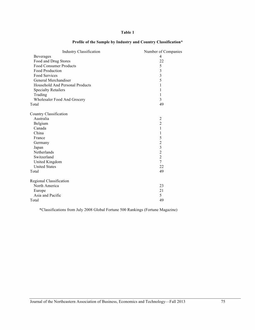
Journal of the Northeastern Association of Business, Economics and Technology—Fall 2013 75
Table 1
Profile of the Sample by Industry and Country Classification*
Industry Classification Number of Companies Beverages 4 Food and Drug Stores 22 Food Consumer Products 5 Food Production 3 Food Services 3 General Merchandiser 5 Household And Personal Products 1 Specialty Retailers 1 Trading 1 Wholesaler Food And Grocery 3 Total 49 Country Classification Australia 2 Belgium 2 Canada 1 China 1 France 5 Germany 2 Japan 3 Netherlands 2 Switzerland 2 United Kingdom 7 United States 22 Total 49 Regional Classification North America 23 Europe 21 Asia and Pacific 5 Total 49 *Classifications from July 2008 Global Fortune 500 Rankings (Fortune Magazine)
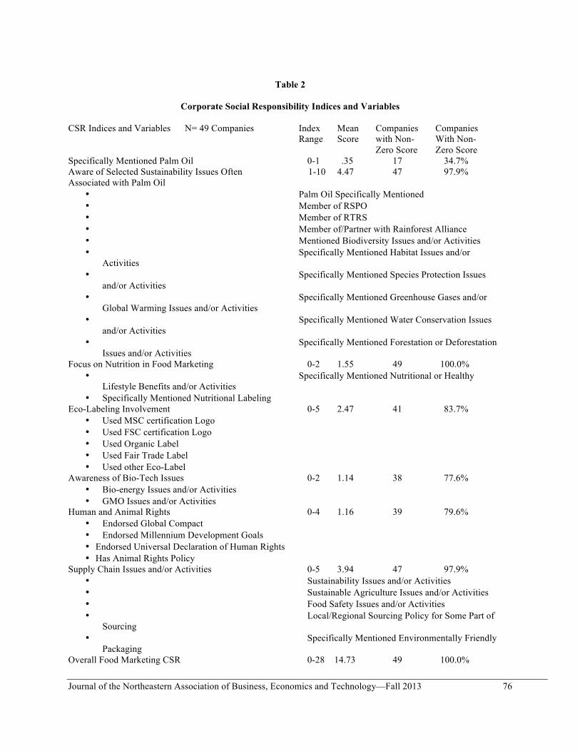
Journal of the Northeastern Association of Business, Economics and Technology—Fall 2013 76
Table 2
Corporate Social Responsibility Indices and Variables
CSR Indices and Variables N= 49 Companies Index Mean Companies Companies Range Score with Non- With Non- Zero Score Zero Score Specifically Mentioned Palm Oil 0-1 .35 17 34.7% Aware of Selected Sustainability Issues Often 1-10 4.47 47 97.9% Associated with Palm Oil
• Palm Oil Specifically Mentioned • Member of RSPO • Member of RTRS • Member of/Partner with Rainforest Alliance • Mentioned Biodiversity Issues and/or Activities • Specifically Mentioned Habitat Issues and/or
Activities • Specifically Mentioned Species Protection Issues
and/or Activities • Specifically Mentioned Greenhouse Gases and/or
Global Warming Issues and/or Activities • Specifically Mentioned Water Conservation Issues
and/or Activities • Specifically Mentioned Forestation or Deforestation
Issues and/or Activities Focus on Nutrition in Food Marketing 0-2 1.55 49 100.0%
• Specifically Mentioned Nutritional or Healthy Lifestyle Benefits and/or Activities
• Specifically Mentioned Nutritional Labeling Eco-Labeling Involvement 0-5 2.47 41 83.7%
• Used MSC certification Logo • Used FSC certification Logo • Used Organic Label • Used Fair Trade Label • Used other Eco-Label
Awareness of Bio-Tech Issues 0-2 1.14 38 77.6% • Bio-energy Issues and/or Activities • GMO Issues and/or Activities
Human and Animal Rights 0-4 1.16 39 79.6% • Endorsed Global Compact • Endorsed Millennium Development Goals • Endorsed Universal Declaration of Human Rights • Has Animal Rights Policy
Supply Chain Issues and/or Activities 0-5 3.94 47 97.9% • Sustainability Issues and/or Activities • Sustainable Agriculture Issues and/or Activities • Food Safety Issues and/or Activities • Local/Regional Sourcing Policy for Some Part of
Sourcing • Specifically Mentioned Environmentally Friendly
Packaging Overall Food Marketing CSR 0-28 14.73 49 100.0%
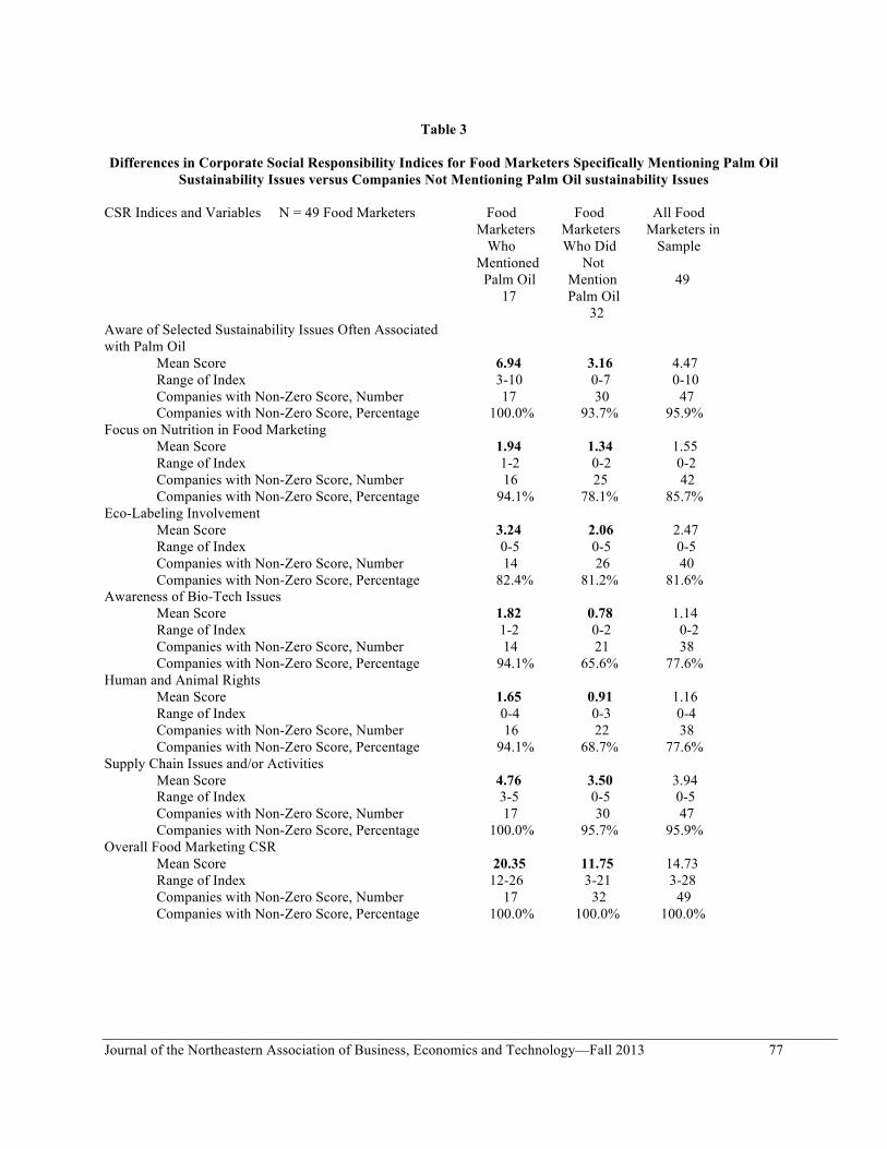
Journal of the Northeastern Association of Business, Economics and Technology—Fall 2013 77
Table 3
Differences in Corporate Social Responsibility Indices for Food Marketers Specifically Mentioning Palm Oil
Sustainability Issues versus Companies Not Mentioning Palm Oil sustainability Issues CSR Indices and Variables N = 49 Food Marketers Food Food All Food Marketers Marketers Marketers in Who Who Did Sample Mentioned Not Palm Oil Mention 49 17 Palm Oil 32 Aware of Selected Sustainability Issues Often Associated with Palm Oil Mean Score 6.94 3.16 4.47 Range of Index 3-10 0-7 0-10 Companies with Non-Zero Score, Number 17 30 47 Companies with Non-Zero Score, Percentage 100.0% 93.7% 95.9% Focus on Nutrition in Food Marketing Mean Score 1.94 1.34 1.55 Range of Index 1-2 0-2 0-2 Companies with Non-Zero Score, Number 16 25 42 Companies with Non-Zero Score, Percentage 94.1% 78.1% 85.7% Eco-Labeling Involvement Mean Score 3.24 2.06 2.47 Range of Index 0-5 0-5 0-5 Companies with Non-Zero Score, Number 14 26 40 Companies with Non-Zero Score, Percentage 82.4% 81.2% 81.6% Awareness of Bio-Tech Issues Mean Score 1.82 0.78 1.14 Range of Index 1-2 0-2 0-2 Companies with Non-Zero Score, Number 14 21 38 Companies with Non-Zero Score, Percentage 94.1% 65.6% 77.6% Human and Animal Rights
Mean Score 1.65 0.91 1.16 Range of Index 0-4 0-3 0-4
Companies with Non-Zero Score, Number 16 22 38 Companies with Non-Zero Score, Percentage 94.1% 68.7% 77.6% Supply Chain Issues and/or Activities Mean Score 4.76 3.50 3.94 Range of Index 3-5 0-5 0-5 Companies with Non-Zero Score, Number 17 30 47 Companies with Non-Zero Score, Percentage 100.0% 95.7% 95.9% Overall Food Marketing CSR Mean Score 20.35 11.75 14.73 Range of Index 12-26 3-21 3-28 Companies with Non-Zero Score, Number 17 32 49 Companies with Non-Zero Score, Percentage 100.0% 100.0% 100.0%
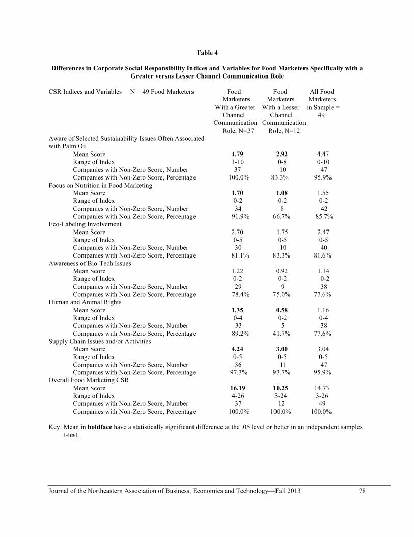
Journal of the Northeastern Association of Business, Economics and Technology—Fall 2013 78
Table 4
Differences in Corporate Social Responsibility Indices and Variables for Food Marketers Specifically with a Greater versus Lesser Channel Communication Role
CSR Indices and Variables N = 49 Food Marketers Food Food All Food Marketers Marketers Marketers With a Greater With a Lesser in Sample = Channel Channel 49 Communication Communication Role, N=37 Role, N=12 Aware of Selected Sustainability Issues Often Associated with Palm Oil Mean Score 4.79 2.92 4.47 Range of Index 1-10 0-8 0-10 Companies with Non-Zero Score, Number 37 10 47 Companies with Non-Zero Score, Percentage 100.0% 83.3% 95.9% Focus on Nutrition in Food Marketing Mean Score 1.70 1.08 1.55 Range of Index 0-2 0-2 0-2 Companies with Non-Zero Score, Number 34 8 42 Companies with Non-Zero Score, Percentage 91.9% 66.7% 85.7% Eco-Labeling Involvement Mean Score 2.70 1.75 2.47 Range of Index 0-5 0-5 0-5 Companies with Non-Zero Score, Number 30 10 40 Companies with Non-Zero Score, Percentage 81.1% 83.3% 81.6% Awareness of Bio-Tech Issues Mean Score 1.22 0.92 1.14 Range of Index 0-2 0-2 0-2 Companies with Non-Zero Score, Number 29 9 38 Companies with Non-Zero Score, Percentage 78.4% 75.0% 77.6% Human and Animal Rights
Mean Score 1.35 0.58 1.16 Range of Index 0-4 0-2 0-4
Companies with Non-Zero Score, Number 33 5 38 Companies with Non-Zero Score, Percentage 89.2% 41.7% 77.6% Supply Chain Issues and/or Activities Mean Score 4.24 3.00 3.04 Range of Index 0-5 0-5 0-5 Companies with Non-Zero Score, Number 36 11 47 Companies with Non-Zero Score, Percentage 97.3% 93.7% 95.9% Overall Food Marketing CSR Mean Score 16.19 10.25 14.73 Range of Index 4-26 3-24 3-26 Companies with Non-Zero Score, Number 37 12 49 Companies with Non-Zero Score, Percentage 100.0% 100.0% 100.0% Key: Mean in boldface have a statistically significant difference at the .05 level or better in an independent samples
t-test.
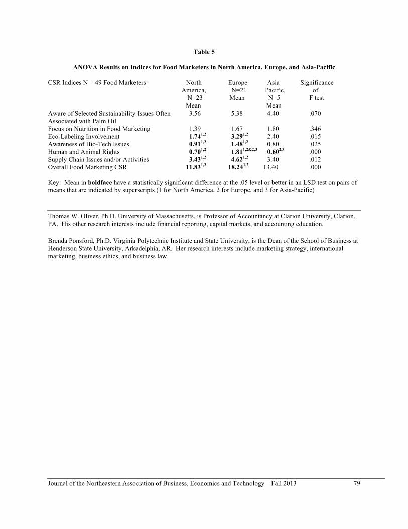
Journal of the Northeastern Association of Business, Economics and Technology—Fall 2013 79
Table 5
ANOVA Results on Indices for Food Marketers in North America, Europe, and Asia-Pacific CSR Indices N = 49 Food Marketers North Europe Asia Significance America, N=21 Pacific, of N=23 Mean N=5 F test Mean Mean Aware of Selected Sustainability Issues Often 3.56 5.38 4.40 .070 Associated with Palm Oil Focus on Nutrition in Food Marketing 1.39 1.67 1.80 .346 Eco-Labeling Involvement 1.741,2 3.291,2 2.40 .015 Awareness of Bio-Tech Issues 0.911,2 1.481,2 0.80 .025 Human and Animal Rights 0.701,2 1.811,2&2,3 0.602,3 .000 Supply Chain Issues and/or Activities 3.431,2 4.621,2 3.40 .012 Overall Food Marketing CSR 11.831,2 18.241,2 13.40 .000 Key: Mean in boldface have a statistically significant difference at the .05 level or better in an LSD test on pairs of means that are indicated by superscripts (1 for North America, 2 for Europe, and 3 for Asia-Pacific)
Thomas W. Oliver, Ph.D. University of Massachusetts, is Professor of Accountancy at Clarion University, Clarion, PA. His other research interests include financial reporting, capital markets, and accounting education.
Brenda Ponsford, Ph.D. Virginia Polytechnic Institute and State University, is the Dean of the School of Business at Henderson State University, Arkadelphia, AR. Her research interests include marketing strategy, international marketing, business ethics, and business law.

JOURNAL OF THE NORTHEASTERN ASSOCIATON OF BUSINESS, ECONOMICS AND TECHNOLOGY


![RJR,NABISCO ANDTH E:'ENWRONMENT - DeSmogBlog · RJR,NABISCO THE RJR NABISCO THIRD ANNUAL ENVIRONMENTAL CONFERENCE Health, Safety and Environmentai Management and R]R Nabisco's Future](https://img.pdfslide.us/doc/110x75/5e7fccea05e8a567bd401713/rjrnabisco-andth-eenwronment-desmogblog-rjrnabisco-the-rjr-nabisco-third-annual.jpg)